PDF generated using the open source mwlib toolkit. See http://code.pediapress.com/ for more information.PDF generated at: Tue, 23 Sep 2014 06:39:34 UTC

Fundamental DataStructures

ContentsArticlesIntroduction 1

Abstract data type 1Data structure 9Analysis of algorithms 12

Sequences 18

Array data type 18Array data structure 22Dynamic array 28

Dictionaries 32

Associative array 32Association list 35Hash table 36Linear probing 49

ReferencesArticle Sources and Contributors 50Image Sources, Licenses and Contributors 52

Article LicensesLicense 53

1

Introduction

Abstract data typeNot to be confused with Algebraic data type.In computer science, an abstract data type (ADT) is a mathematical model for a certain class of data structures thathave similar behavior; or for certain data types of one or more programming languages that have similar semantics.An abstract data type is defined indirectly, only by the operations that may be performed on it and by mathematicalconstraints on the effects (and possibly cost) of those operations.[1]

For example, an abstract stack could be defined by three operations: push, that inserts some data item onto thestructure, pop, that extracts an item from it (with the constraint that each pop always returns the most recentlypushed item that has not been popped yet), and peek, that allows data on top of the structure to be examined withoutremoval. When analyzing the efficiency of algorithms that use stacks, one may also specify that all operations takethe same time no matter how many items have been pushed into the stack, and that the stack uses a constant amountof storage for each element.Abstract data types are purely theoretical entities, used (among other things) to simplify the description of abstractalgorithms, to classify and evaluate data structures, and to formally describe the type systems of programminglanguages. However, an ADT may be implemented by specific data types or data structures, in many ways and inmany programming languages; or described in a formal specification language. ADTs are often implemented asmodules: the module's interface declares procedures that correspond to the ADT operations, sometimes withcomments that describe the constraints. This information hiding strategy allows the implementation of the module tobe changed without disturbing the client programs.The term abstract data type can also be regarded as a generalised approach of a number of algebraic structures,such as lattices, groups, and rings.[2] This can be treated as part of the subject area of artificial intelligence. Thenotion of abstract data types is related to the concept of data abstraction, important in object-oriented programmingand design by contract methodologies for software development Wikipedia:Citation needed.

Defining an abstract data type (ADT)An abstract data type is defined as a mathematical model of the data objects that make up a data type as well as thefunctions that operate on these objects. There are no standard conventions for defining them. A broad division maybe drawn between "imperative" and "functional" definition styles.

IB Computer Science Abstract Data TypeIn the course an abstract data type refers to a generalised data structure that accepts data objects stored as a list withspecific behaviours defined by the methods associated with the underlying nature of the list.This is a very important BIG idea in computer science. It is based on the recognitation that often a group of data issimply a list in random or some specific order. A list of numbers can be either integer or real but as in arithmetic thenumbers can represent any numeric quantity e.g. weight of a list of students in a classroom, in which case we wouldhave a list of real numbers. Mathematical operations e.g. average, min, max are performed exactly the same way onany list of real numbers irrespective of the specific concrete nature of the list.For example: a group of people queueing at the canteen can be represented as a list with certain characteristics orbehaviours. People arrive and attach to the end of the queue, people get served and leave the queue from the head or

Abstract data type 2

start of the queue. Any simple queue can be described in exactly the same way. The same basic operations: add,remove, insert are always the same, it does not matter that the data object represent a person or something else.Adding the object to end of the queue is exactly the same operation for any set of data described as a queue.An ADT has a generalised name e.g. Stack, Queue, BinaryTree etc. Each ADT accepts data objects that arerepresented as members of the underlying list e.g. an integer, a Person Object. Each ADT has a set of pre-definedmethods (behaviours in OOPs terminology) that can be used to manipulate the members in the list - irrespective ofwhat they actually in reality represent.Other specific ADT material can be found in specific Wikipedia sections e.g. Stack, Queue, Array etc.

Imperative viewIn the "imperative" view, which is closer to the philosophy of imperative programming languages, an abstract datastructure is conceived as an entity that is mutable — meaning that it may be in different states at different times.Some operations may change the state of the ADT; therefore, the order in which operations are evaluated isimportant, and the same operation on the same entities may have different effects if executed at different times —just like the instructions of a computer, or the commands and procedures of an imperative language. To underscorethis view, it is customary to say that the operations are executed or applied, rather than evaluated. The imperativestyle is often used when describing abstract algorithms. This is described by Donald E. Knuth and can be referencedfrom here The Art of Computer Programming.

Abstract variable

Imperative ADT definitions often depend on the concept of an abstract variable, which may be regarded as thesimplest non-trivial ADT. An abstract variable V is a mutable entity that admits two operations:• store(V,x) where x is a value of unspecified nature; and• fetch(V), that yields a value;with the constraint that• fetch(V) always returns the value x used in the most recent store(V,x) operation on the same variable V.As in so many programming languages, the operation store(V,x) is often written V ← x (or some similar notation),and fetch(V) is implied whenever a variable V is used in a context where a value is required. Thus, for example, V← V + 1 is commonly understood to be a shorthand for store(V,fetch(V) + 1).In this definition, it is implicitly assumed that storing a value into a variable U has no effect on the state of a distinctvariable V. To make this assumption explicit, one could add the constraint that• if U and V are distinct variables, the sequence { store(U,x); store(V,y) } is equivalent to { store(V,y);store(U,x) }.

More generally, ADT definitions often assume that any operation that changes the state of one ADT instance has noeffect on the state of any other instance (including other instances of the same ADT) — unless the ADT axiomsimply that the two instances are connected (aliased) in that sense. For example, when extending the definition ofabstract variable to include abstract records, the operation that selects a field from a record variable R must yield avariable V that is aliased to that part of R.The definition of an abstract variable V may also restrict the stored values x to members of a specific set X, called therange or type of V. As in programming languages, such restrictions may simplify the description and analysis ofalgorithms, and improve their readability.Note that this definition does not imply anything about the result of evaluating fetch(V) when V is un-initialized, that is, before performing any store operation on V. An algorithm that does so is usually considered invalid, because its effect is not defined. (However, there are some important algorithms whose efficiency strongly depends on the assumption that such a fetch is legal, and returns some arbitrary value in the variable's

Abstract data type 3

range.Wikipedia:Citation needed)

Instance creation

Some algorithms need to create new instances of some ADT (such as new variables, or new stacks). To describesuch algorithms, one usually includes in the ADT definition a create() operation that yields an instance of theADT, usually with axioms equivalent to• the result of create() is distinct from any instance S in use by the algorithm.This axiom may be strengthened to exclude also partial aliasing with other instances. On the other hand, this axiomstill allows implementations of create() to yield a previously created instance that has become inaccessible to theprogram.

Preconditions, postconditions, and invariants

In imperative-style definitions, the axioms are often expressed by preconditions, that specify when an operation maybe executed; postconditions, that relate the states of the ADT before and after the execution of each operation; andinvariants, that specify properties of the ADT that are not changed by the operations.

Example: abstract stack (imperative)

As another example, an imperative definition of an abstract stack could specify that the state of a stack S can bemodified only by the operations• push(S,x), where x is some value of unspecified nature; and• pop(S), that yields a value as a result;with the constraint that• For any value x and any abstract variable V, the sequence of operations { push(S,x); V ← pop(S) } is equivalent

to { V ← x };Since the assignment { V ← x }, by definition, cannot change the state of S, this condition implies that { V ←pop(S) } restores S to the state it had before the { push(S,x) }. From this condition and from the properties ofabstract variables, it follows, for example, that the sequence

{ push(S,x); push(S,y); U ← pop(S); push(S,z); V ← pop(S); W ← pop(S); }where x,y, and z are any values, and U, V, W are pairwise distinct variables, is equivalent to

{ U ← y; V ← z; W ← x }Here it is implicitly assumed that operations on a stack instance do not modify the state of any other ADT instance,including other stacks; that is,• For any values x,y, and any distinct stacks S and T, the sequence { push(S,x); push(T,y) } is equivalent to {push(T,y); push(S,x) }.

A stack ADT definition usually includes also a Boolean-valued function empty(S) and a create() operation thatreturns a stack instance, with axioms equivalent to• create() ≠ S for any stack S (a newly created stack is distinct from all previous stacks)• empty(create()) (a newly created stack is empty)• not empty(push(S,x)) (pushing something into a stack makes it non-empty)

Abstract data type 4

Single-instance style

Sometimes an ADT is defined as if only one instance of it existed during the execution of the algorithm, and alloperations were applied to that instance, which is not explicitly notated. For example, the abstract stack above couldhave been defined with operations push(x) and pop(), that operate on "the" only existing stack. ADT definitions inthis style can be easily rewritten to admit multiple coexisting instances of the ADT, by adding an explicit instanceparameter (like S in the previous example) to every operation that uses or modifies the implicit instance.On the other hand, some ADTs cannot be meaningfully defined without assuming multiple instances. This is the casewhen a single operation takes two distinct instances of the ADT as parameters. For an example, consider augmentingthe definition of the stack ADT with an operation compare(S,T) that checks whether the stacks S and T contain thesame items in the same order.

Functional ADT definitionsAnother way to define an ADT, closer to the spirit of functional programming, is to consider each state of thestructure as a separate entity. In this view, any operation that modifies the ADT is modeled as a mathematicalfunction that takes the old state as an argument, and returns the new state as part of the result. Unlike the"imperative" operations, these functions have no side effects. Therefore, the order in which they are evaluated isimmaterial, and the same operation applied to the same arguments (including the same input states) will alwaysreturn the same results (and output states).In the functional view, in particular, there is no way (or need) to define an "abstract variable" with the semantics ofimperative variables (namely, with fetch and store operations). Instead of storing values into variables, onepasses them as arguments to functions.

Example: abstract stack (functional)

For example, a complete functional-style definition of a stack ADT could use the three operations:• push: takes a stack state and an arbitrary value, returns a stack state;• top: takes a stack state, returns a value;• pop: takes a stack state, returns a stack state;In a functional-style definition there is no need for a create operation. Indeed, there is no notion of "stackinstance". The stack states can be thought of as being potential states of a single stack structure, and two stack statesthat contain the same values in the same order are considered to be identical states. This view actually mirrors thebehavior of some concrete implementations, such as linked lists with hash cons.Instead of create(), a functional definition of a stack ADT may assume the existence of a special stack state, theempty stack, designated by a special symbol like Λ or "()"; or define a bottom() operation that takes no argumentsand returns this special stack state. Note that the axioms imply that• push(Λ,x) ≠ ΛIn a functional definition of a stack one does not need an empty predicate: instead, one can test whether a stack isempty by testing whether it is equal to Λ.Note that these axioms do not define the effect of top(s) or pop(s), unless s is a stack state returned by a push.Since push leaves the stack non-empty, those two operations are undefined (hence invalid) when s = Λ. On theother hand, the axioms (and the lack of side effects) imply that push(s,x) = push(t,y) if and only if x = y and s = t.As in some other branches of mathematics, it is customary to assume also that the stack states are only those whose existence can be proved from the axioms in a finite number of steps. In the stack ADT example above, this rule means that every stack is a finite sequence of values, that becomes the empty stack (Λ) after a finite number of pops. By themselves, the axioms above do not exclude the existence of infinite stacks (that can be poped forever, each time yielding a different state) or circular stacks (that return to the same state after a finite number of pops). In

Abstract data type 5

particular, they do not exclude states s such that pop(s) = s or push(s,x) = s for some x. However, since one cannotobtain such stack states with the given operations, they are assumed "not to exist".

Advantages of abstract data typing•• EncapsulationAbstraction provides a promise that any implementation of the ADT has certain properties and abilities; knowingthese is all that is required to make use of an ADT object. The user does not need any technical knowledge of howthe implementation works to use the ADT. In this way, the implementation may be complex but will be encapsulatedin a simple interface when it is actually used.•• Localization of changeCode that uses an ADT object will not need to be edited if the implementation of the ADT is changed. Since anychanges to the implementation must still comply with the interface, and since code using an ADT may only refer toproperties and abilities specified in the interface, changes may be made to the implementation without requiring anychanges in code where the ADT is used.•• FlexibilityDifferent implementations of an ADT, having all the same properties and abilities, are equivalent and may be usedsomewhat interchangeably in code that uses the ADT. This gives a great deal of flexibility when using ADT objectsin different situations. For example, different implementations of an ADT may be more efficient in differentsituations; it is possible to use each in the situation where they are preferable, thus increasing overall efficiency.

Typical operationsSome operations that are often specified for ADTs (possibly under other names) are• compare(s,t), that tests whether two structures are equivalent in some sense;• hash(s), that computes some standard hash function from the instance's state;• print(s) or show(s), that produces a human-readable representation of the structure's state.In imperative-style ADT definitions, one often finds also• create(), that yields a new instance of the ADT;• initialize(s), that prepares a newly created instance s for further operations, or resets it to some "initial

state";• copy(s,t), that puts instance s in a state equivalent to that of t;• clone(t), that performs s ← create(), copy(s,t), and returns s;• free(s) or destroy(s), that reclaims the memory and other resources used by s;The free operation is not normally relevant or meaningful, since ADTs are theoretical entities that do not "usememory". However, it may be necessary when one needs to analyze the storage used by an algorithm that uses theADT. In that case one needs additional axioms that specify how much memory each ADT instance uses, as afunction of its state, and how much of it is returned to the pool by free.

Abstract data type 6

ExamplesSome common ADTs, which have proved useful in a great variety of applications, are•• Container•• Deque•• List•• Map•• Multimap•• Multiset•• Priority queue•• Queue•• Set•• Stack•• Tree•• GraphEach of these ADTs may be defined in many ways and variants, not necessarily equivalent. For example, a stackADT may or may not have a count operation that tells how many items have been pushed and not yet popped.This choice makes a difference not only for its clients but also for the implementation.

ImplementationImplementing an ADT means providing one procedure or function for each abstract operation. The ADT instancesare represented by some concrete data structure that is manipulated by those procedures, according to the ADT'sspecifications.Usually there are many ways to implement the same ADT, using several different concrete data structures. Thus, forexample, an abstract stack can be implemented by a linked list or by an array.An ADT implementation is often packaged as one or more modules, whose interface contains only the signature(number and types of the parameters and results) of the operations. The implementation of the module — namely,the bodies of the procedures and the concrete data structure used — can then be hidden from most clients of themodule. This makes it possible to change the implementation without affecting the clients.When implementing an ADT, each instance (in imperative-style definitions) or each state (in functional-styledefinitions) is usually represented by a handle of some sort.[3]

Modern object-oriented languages, such as C++ and Java, support a form of abstract data types. When a class is usedas a type, it is an abstract type that refers to a hidden representation. In this model an ADT is typically implementedas a class, and each instance of the ADT is usually an object of that class. The module's interface typically declaresthe constructors as ordinary procedures, and most of the other ADT operations as methods of that class. However,such an approach does not easily encapsulate multiple representational variants found in an ADT. It also canundermine the extensibility of object-oriented programs. In a pure object-oriented program that uses interfaces astypes, types refer to behaviors not representations.

Abstract data type 7

Example: implementation of the stack ADTAs an example, here is an implementation of the stack ADT above in the C programming language.Imperative-style interface

An imperative-style interface might be:

typedef struct stack_Rep stack_Rep; /* Type: instance

representation (an opaque record). */

typedef stack_Rep *stack_T; /* Type: handle to a stack

instance (an opaque pointer). */

typedef void *stack_Item; /* Type: value that can be

stored in stack (arbitrary address). */

stack_T stack_create(void); /* Create new stack

instance, initially empty. */

void stack_push(stack_T s, stack_Item e); /* Add an item at the top of

the stack. */

stack_Item stack_pop(stack_T s); /* Remove the top item from

the stack and return it . */

int stack_empty(stack_T ts); /* Check whether stack is

empty. */

This implementation could be used in the following manner:

#include <stack.h> /* Include the stack interface. */

stack_T t = stack_create(); /* Create a stack instance. */

int foo = 17; /* An arbitrary datum. */

stack_push(t, &foo); /* Push the address of 'foo' onto the

stack. */

…void *e = stack_pop(t); /* Get the top item and delete it from

the stack. */

if (stack_empty(t)) { … } /* Do something if stack is empty. */…

This interface can be implemented in many ways. The implementation may be arbitrarily inefficient, since the formaldefinition of the ADT, above, does not specify how much space the stack may use, nor how long each operationshould take. It also does not specify whether the stack state t continues to exist after a call s ← pop(t).In practice the formal definition should specify that the space is proportional to the number of items pushed and notyet popped; and that every one of the operations above must finish in a constant amount of time, independently ofthat number. To comply with these additional specifications, the implementation could use a linked list, or an array(with dynamic resizing) together with two integers (an item count and the array size)

Abstract data type 8

Functional-style interface

Functional-style ADT definitions are more appropriate for functional programming languages, and vice-versa.However, one can provide a functional style interface even in an imperative language like C. For example:

typedef struct stack_Rep stack_Rep; /* Type: stack state

representation (an opaque record). */

typedef stack_Rep *stack_T; /* Type: handle to a stack

state (an opaque pointer). */

typedef void *stack_Item; /* Type: item (arbitrary

address). */

stack_T stack_empty(void); /* Returns the empty stack

state. */

stack_T stack_push(stack_T s, stack_Item x); /* Adds x at the top of s,

returns the resulting state. */

stack_Item stack_top(stack_T s); /* Returns the item

currently at the top of s. */

stack_T stack_pop(stack_T s); /* Remove the top item

from s, returns the resulting state. */

The main problem is that C lacks garbage collection, and this makes this style of programming impractical;moreover, memory allocation routines in C are slower than allocation in a typical garbage collector, thus theperformance impact of so many allocations is even greater.

ADT librariesMany modern programming languages, such as C++ and Java, come with standard libraries that implement severalcommon ADTs, such as those listed above.

Built-in abstract data typesThe specification of some programming languages is intentionally vague about the representation of certain built-indata types, defining only the operations that can be done on them. Therefore, those types can be viewed as "built-inADTs". Examples are the arrays in many scripting languages, such as Awk, Lua, and Perl, which can be regarded asan implementation of the Map or Table ADT.

References[1] Barbara Liskov, Programming with Abstract Data Types, in Proceedings of the ACM SIGPLAN Symposium on Very High Level Languages,

pp. 50--59, 1974, Santa Monica, California[2][2] , Chapter 7,section 40.[3][3] , definition 4.4.

Further• Mitchell, John C.; Plotkin, Gordon (July 1988). "Abstract Types Have Existential Type" (http:/ / theory. stanford.

edu/ ~jcm/ papers/ mitch-plotkin-88. pdf). ACM Transactions on Programming Languages and Systems 10 (3).

Abstract data type 9

External links• Abstract data type (http:/ / www. nist. gov/ dads/ HTML/ abstractDataType. html) in NIST Dictionary of

Algorithms and Data Structures• Walls and Mirrors, the classic textbook

Data structure

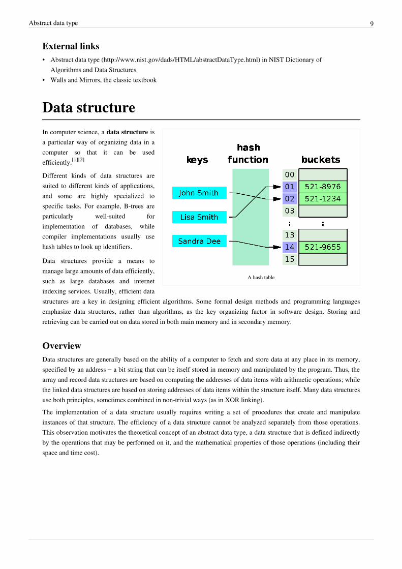
A hash table

In computer science, a data structure isa particular way of organizing data in acomputer so that it can be usedefficiently.[1][2]

Different kinds of data structures aresuited to different kinds of applications,and some are highly specialized tospecific tasks. For example, B-trees areparticularly well-suited forimplementation of databases, whilecompiler implementations usually usehash tables to look up identifiers.

Data structures provide a means tomanage large amounts of data efficiently,such as large databases and internetindexing services. Usually, efficient datastructures are a key in designing efficient algorithms. Some formal design methods and programming languagesemphasize data structures, rather than algorithms, as the key organizing factor in software design. Storing andretrieving can be carried out on data stored in both main memory and in secondary memory.

OverviewData structures are generally based on the ability of a computer to fetch and store data at any place in its memory,specified by an address – a bit string that can be itself stored in memory and manipulated by the program. Thus, thearray and record data structures are based on computing the addresses of data items with arithmetic operations; whilethe linked data structures are based on storing addresses of data items within the structure itself. Many data structuresuse both principles, sometimes combined in non-trivial ways (as in XOR linking).The implementation of a data structure usually requires writing a set of procedures that create and manipulateinstances of that structure. The efficiency of a data structure cannot be analyzed separately from those operations.This observation motivates the theoretical concept of an abstract data type, a data structure that is defined indirectlyby the operations that may be performed on it, and the mathematical properties of those operations (including theirspace and time cost).

Data structure 10

ExamplesMain article: List of data structuresThere are numerous types of data structures:• An array is a number of elements in a specific order. They are accessed using an integer to specify which element

is required (although the elements may be of almost any type). Typical implementations allocate contiguousmemory words for the elements of arrays (but this is not always a necessity). Arrays may be fixed-length orexpandable.

• Records (also called tuples or structs) are among the simplest data structures. A record is a value that containsother values, typically in fixed number and sequence and typically indexed by names. The elements of records areusually called fields or members.

• An associative array (also called a dictionary or map) is a more flexible variation on a record, in whichname-value pairs can be added and deleted freely. A hash table is a common implementation of an associativearray.

• A union type specifies which of a number of permitted primitive types may be stored in its instances, e.g. "float orlong integer". Contrast with a record, which could be defined to contain a float and an integer; whereas, in aunion, there is only one value at a time. Enough space is allocated to contain the widest member datatype.

• A tagged union (also called a variant, variant record, discriminated union, or disjoint union) contains anadditional field indicating its current type, for enhanced type safety.

• A set is an abstract data structure that can store specific values, without any particular order, and with no repeatedvalues. Values themselves are not retrieved from sets, rather one tests a value for membership to obtain a boolean"in" or "not in".

• Graphs and trees are linked abstract data structures composed of nodes. Each node contains a value and also oneor more pointers to other nodes. Graphs can be used to represent networks, while variants of trees can be used forsorting and searching, having their nodes arranged in some relative order based on their values.

• An object contains data fields, like a record, as well as various methods. In the context of object-orientedprogramming, records are known as plain old data structures to distinguish them from objects.

Language supportMost assembly languages and some low-level languages, such as BCPL (Basic Combined Programming Language),lack support for data structures. On the other hand, many high-level programming languages and some higher-levelassembly languages, such as MASM, have special syntax or other built-in support for certain data structures, such asrecords and arrays. For example, the C and Pascal languages support structs and records, respectively, in addition tovectors (one-dimensional arrays) and multi-dimensional arrays.Most programming languages feature some sort of library mechanism that allows data structure implementations tobe reused by different programs. Modern languages usually come with standard libraries that implement the mostcommon data structures. Examples are the C++ Standard Template Library, the Java Collections Framework, andMicrosoft's .NET Framework.Modern languages also generally support modular programming, the separation between the interface of a librarymodule and its implementation. Some provide opaque data types that allow clients to hide implementation details.Object-oriented programming languages, such as C++, Java and Smalltalk may use classes for this purpose.Many known data structures have concurrent versions that allow multiple computing threads to access the datastructure simultaneously.

Data structure 11

References[1] Paul E. Black (ed.), entry for data structure in Dictionary of Algorithms and Data Structures. U.S. National Institute of Standards and

Technology. 15 December 2004. Online version (http:/ / xlinux. nist. gov/ dads/ HTML/ datastructur. html) Accessed May 21, 2009.[2] Entry data structure in the Encyclopædia Britannica (2009) Online entry (http:/ / www. britannica. com/ EBchecked/ topic/ 152190/

data-structure) accessed on May 21, 2009.

Further reading• Peter Brass, Advanced Data Structures, Cambridge University Press, 2014• Donald Knuth, The Art of Computer Programming, vol. 1. Addison-Wesley, 3rd edition, 1997.• Dinesh Mehta and Sartaj Sahni Handbook of Data Structures and Applications, Chapman and Hall/CRC Press,

2007.• Niklaus Wirth, Algorithms and Data Structures, Prentice Hall, 1985.•• Diane Zak, Introduction to programming with c++, copyright 2011 Cengage Learning Asia Pte Ltd

External links• course on data structures (http:/ / scanftree. com/ Data_Structure/ )• Data structures Programs Examples in c,java (http:/ / scanftree. com/ programs/ operation/ data-structure/ )• UC Berkeley video course on data structures (http:/ / academicearth. org/ computer-science/ )• Descriptions (http:/ / nist. gov/ dads/ ) from the Dictionary of Algorithms and Data Structures• Data structures course (http:/ / www. cs. auckland. ac. nz/ software/ AlgAnim/ ds_ToC. html)• An Examination of Data Structures from .NET perspective (http:/ / msdn. microsoft. com/ en-us/ library/

aa289148(VS. 71). aspx)• Schaffer, C. Data Structures and Algorithm Analysis (http:/ / people. cs. vt. edu/ ~shaffer/ Book/ C+ +

3e20110915. pdf)

Analysis of algorithms 12

Analysis of algorithmsIn computer science, the analysis of algorithms is the determination of the amount of resources (such as time andstorage) necessary to execute them. Most algorithms are designed to work with inputs of arbitrary length. Usually,the efficiency or running time of an algorithm is stated as a function relating the input length to the number of steps(time complexity) or storage locations (space complexity).Algorithm analysis is an important part of a broader computational complexity theory, which provides theoreticalestimates for the resources needed by any algorithm which solves a given computational problem. These estimatesprovide an insight into reasonable directions of search for efficient algorithms.In theoretical analysis of algorithms it is common to estimate their complexity in the asymptotic sense, i.e., toestimate the complexity function for arbitrarily large input. Big O notation, Big-omega notation and Big-thetanotation are used to this end. For instance, binary search is said to run in a number of steps proportional to thelogarithm of the length of the list being searched, or in O(log(n)), colloquially "in logarithmic time". Usuallyasymptotic estimates are used because different implementations of the same algorithm may differ in efficiency.However the efficiencies of any two "reasonable" implementations of a given algorithm are related by a constantmultiplicative factor called a hidden constant.Exact (not asymptotic) measures of efficiency can sometimes be computed but they usually require certainassumptions concerning the particular implementation of the algorithm, called model of computation. A model ofcomputation may be defined in terms of an abstract computer, e.g., Turing machine, and/or by postulating thatcertain operations are executed in unit time. For example, if the sorted list to which we apply binary search has nelements, and we can guarantee that each lookup of an element in the list can be done in unit time, then at most log2n + 1 time units are needed to return an answer.

Cost modelsTime efficiency estimates depend on what we define to be a step. For the analysis to correspond usefully to theactual execution time, the time required to perform a step must be guaranteed to be bounded above by a constant.One must be careful here; for instance, some analyses count an addition of two numbers as one step. This assumptionmay not be warranted in certain contexts. For example, if the numbers involved in a computation may be arbitrarilylarge, the time required by a single addition can no longer be assumed to be constant.Two cost models are generally used:[1]

• the uniform cost model, also called uniform-cost measurement (and similar variations), assigns a constant costto every machine operation, regardless of the size of the numbers involved

• the logarithmic cost model, also called logarithmic-cost measurement (and variations thereof), assigns a cost toevery machine operation proportional to the number of bits involved

The latter is more cumbersome to use, so it's only employed when necessary, for example in the analysis ofarbitrary-precision arithmetic algorithms, like those used in cryptography.A key point which is often overlooked is that published lower bounds for problems are often given for a model ofcomputation that is more restricted than the set of operations that you could use in practice and therefore there arealgorithms that are faster than what would naively be thought possible.[2]

Analysis of algorithms 13

Run-time analysisRun-time analysis is a theoretical classification that estimates and anticipates the increase in running time (orrun-time) of an algorithm as its input size (usually denoted as n) increases. Run-time efficiency is a topic of greatinterest in computer science: A program can take seconds, hours or even years to finish executing, depending onwhich algorithm it implements (see also performance analysis, which is the analysis of an algorithm's run-time inpractice).

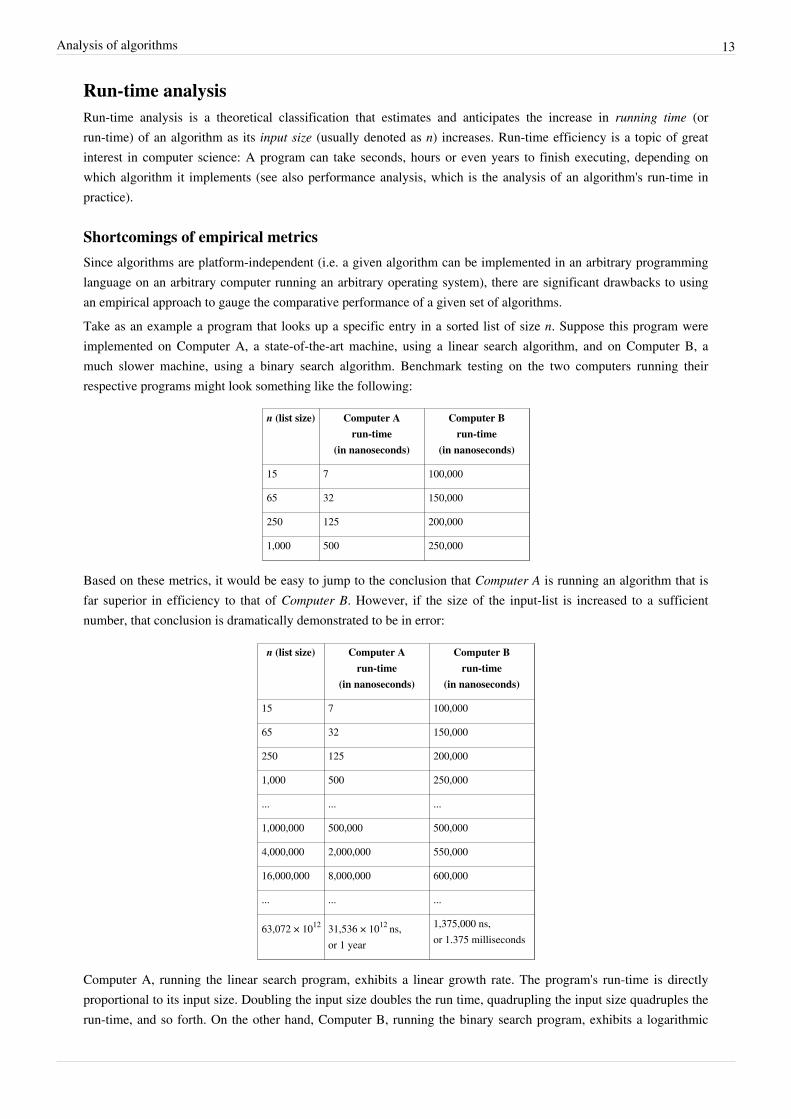
Shortcomings of empirical metricsSince algorithms are platform-independent (i.e. a given algorithm can be implemented in an arbitrary programminglanguage on an arbitrary computer running an arbitrary operating system), there are significant drawbacks to usingan empirical approach to gauge the comparative performance of a given set of algorithms.Take as an example a program that looks up a specific entry in a sorted list of size n. Suppose this program wereimplemented on Computer A, a state-of-the-art machine, using a linear search algorithm, and on Computer B, amuch slower machine, using a binary search algorithm. Benchmark testing on the two computers running theirrespective programs might look something like the following:

n (list size) Computer Arun-time

(in nanoseconds)

Computer Brun-time

(in nanoseconds)

15 7 100,000

65 32 150,000

250 125 200,000

1,000 500 250,000

Based on these metrics, it would be easy to jump to the conclusion that Computer A is running an algorithm that isfar superior in efficiency to that of Computer B. However, if the size of the input-list is increased to a sufficientnumber, that conclusion is dramatically demonstrated to be in error:

n (list size) Computer Arun-time

(in nanoseconds)

Computer Brun-time

(in nanoseconds)

15 7 100,000

65 32 150,000

250 125 200,000

1,000 500 250,000

... ... ...

1,000,000 500,000 500,000

4,000,000 2,000,000 550,000

16,000,000 8,000,000 600,000

... ... ...

63,072 × 1012 31,536 × 1012 ns,or 1 year

1,375,000 ns,or 1.375 milliseconds

Computer A, running the linear search program, exhibits a linear growth rate. The program's run-time is directly proportional to its input size. Doubling the input size doubles the run time, quadrupling the input size quadruples the run-time, and so forth. On the other hand, Computer B, running the binary search program, exhibits a logarithmic

Analysis of algorithms 14

growth rate. Doubling the input size only increases the run time by a constant amount (in this example, 50,000 ns).Even though Computer A is ostensibly a faster machine, Computer B will inevitably surpass Computer A in run-timebecause it's running an algorithm with a much slower growth rate.

Orders of growthMain article: Big O notationInformally, an algorithm can be said to exhibit a growth rate on the order of a mathematical function if beyond acertain input size n, the function f(n) times a positive constant provides an upper bound or limit for the run-time ofthat algorithm. In other words, for a given input size n greater than some n0 and a constant c, the running time of thatalgorithm will never be larger than c × f(n). This concept is frequently expressed using Big O notation. For example,since the run-time of insertion sort grows quadratically as its input size increases, insertion sort can be said to be oforder O(n²).Big O notation is a convenient way to express the worst-case scenario for a given algorithm, although it can also beused to express the average-case — for example, the worst-case scenario for quicksort is O(n²), but the average-caserun-time is O(n log n).[3]

Empirical orders of growthAssuming the execution time follows power rule, t ≈ k na, the coefficient a can be found [4] by taking empiricalmeasurements of run time at some problem-size points , and calculating so that . If the order of growth indeed follows the power rule, the empirical valueof a will stay constant at different ranges, and if not, it will change - but still could serve for comparison of any twogiven algorithms as to their empirical local orders of growth behaviour. Applied to the above table:

n (list size) Computer Arun-time

(in nanoseconds)

Local order ofgrowth(n^_)

Computer Brun-time

(in nanoseconds)

Local order ofgrowth(n^_)

15 7 100,000

65 32 1.04 150,000 0.28

250 125 1.01 200,000 0.21

1,000 500 1.00 250,000 0.16

... ... ...

1,000,000 500,000 1.00 500,000 0.10

4,000,000 2,000,000 1.00 550,000 0.07

16,000,000 8,000,000 1.00 600,000 0.06

... ... ...

It is clearly seen that the first algorithm exhibits a linear order of growth indeed following the power rule. Theempirical values for the second one are diminishing rapidly, suggesting it follows another rule of growth and in anycase has much lower local orders of growth (and improving further still), empirically, than the first one.

Analysis of algorithms 15

Evaluating run-time complexityThe run-time complexity for the worst-case scenario of a given algorithm can sometimes be evaluated by examiningthe structure of the algorithm and making some simplifying assumptions. Consider the following pseudocode:

1 get a positive integer from input

2 if n > 10

3 print "This might take a while..."

4 for i = 1 to n

5 for j = 1 to i

6 print i * j

7 print "Done!"

A given computer will take a discrete amount of time to execute each of the instructions involved with carrying outthis algorithm. The specific amount of time to carry out a given instruction will vary depending on which instructionis being executed and which computer is executing it, but on a conventional computer, this amount will bedeterministic.[5] Say that the actions carried out in step 1 are considered to consume time T1, step 2 uses time T2, andso forth.In the algorithm above, steps 1, 2 and 7 will only be run once. For a worst-case evaluation, it should be assumed thatstep 3 will be run as well. Thus the total amount of time to run steps 1-3 and step 7 is:

The loops in steps 4, 5 and 6 are trickier to evaluate. The outer loop test in step 4 will execute ( n + 1 ) times (notethat an extra step is required to terminate the for loop, hence n + 1 and not n executions), which will consume T4( n +1 ) time. The inner loop, on the other hand, is governed by the value of i, which iterates from 1 to i. On the first passthrough the outer loop, j iterates from 1 to 1: The inner loop makes one pass, so running the inner loop body (step 6)consumes T6 time, and the inner loop test (step 5) consumes 2T5 time. During the next pass through the outer loop, jiterates from 1 to 2: the inner loop makes two passes, so running the inner loop body (step 6) consumes 2T6 time,and the inner loop test (step 5) consumes 3T5 time.Altogether, the total time required to run the inner loop body can be expressed as an arithmetic progression:

which can be factored[6] as

The total time required to run the outer loop test can be evaluated similarly:

which can be factored as

Therefore the total running time for this algorithm is:

which reduces to

As a rule-of-thumb, one can assume that the highest-order term in any given function dominates its rate of growth and thus defines its run-time order. In this example, n² is the highest-order term, so one can conclude that f(n) =

Analysis of algorithms 16

O(n²). Formally this can be proven as follows:

Prove that

(for n ≥ 0)Let k be a constant greater than or equal to [T1..T7]

(for n ≥ 1)

Therefore

for A more elegant approach to analyzing this algorithm would be to declare that [T1..T7] are all equal to one unit oftime, in a system of units chosen so that one unit is greater than or equal to the actual times for these steps. Thiswould mean that the algorithm's running time breaks down as follows:[7]

(for n ≥ 1)

Growth rate analysis of other resourcesThe methodology of run-time analysis can also be utilized for predicting other growth rates, such as consumption ofmemory space. As an example, consider the following pseudocode which manages and reallocates memory usage bya program based on the size of a file which that program manages:

while (file still open)

let n = size of file

for every 100,000 kilobytes of increase in file size

double the amount of memory reserved

In this instance, as the file size n increases, memory will be consumed at an exponential growth rate, which is orderO(2n). This is an extremely rapid and most likely unmanageable growth rate for consumption of memory resources.

RelevanceAlgorithm analysis is important in practice because the accidental or unintentional use of an inefficient algorithm cansignificantly impact system performance. In time-sensitive applications, an algorithm taking too long to run canrender its results outdated or useless. An inefficient algorithm can also end up requiring an uneconomical amount ofcomputing power or storage in order to run, again rendering it practically useless.

Notes[1][1] , section 1.3[2] Examples of the price of abstraction? (http:/ / cstheory. stackexchange. com/ questions/ 608/ examples-of-the-price-of-abstraction),

cstheory.stackexchange.com[3] The term lg is often used as shorthand for log2[4] How To Avoid O-Abuse and Bribes (http:/ / rjlipton. wordpress. com/ 2009/ 07/ 24/ how-to-avoid-o-abuse-and-bribes/ ), at the blog "Gödel’s

Lost Letter and P=NP" by R. J. Lipton, professor of Computer Science at Georgia Tech, recounting idea by Robert Sedgewick[5] However, this is not the case with a quantum computer[6] It can be proven by induction that UNIQ-math-0-af19578567ebd1f4-QINU[7] This approach, unlike the above approach, neglects the constant time consumed by the loop tests which terminate their respective loops, but it

is trivial to prove that such omission does not affect the final result

Analysis of algorithms 17

References• Cormen, Thomas H.; Leiserson, Charles E.; Rivest, Ronald L. & Stein, Clifford (2001). Introduction to

Algorithms. Chapter 1: Foundations (Second ed.). Cambridge, MA: MIT Press and McGraw-Hill. pp. 3–122.ISBN 0-262-03293-7.

• Sedgewick, Robert (1998). Algorithms in C, Parts 1-4: Fundamentals, Data Structures, Sorting, Searching (3rded.). Reading, MA: Addison-Wesley Professional. ISBN 978-0-201-31452-6.

• Knuth, Donald. The Art of Computer Programming. Addison-Wesley.• Greene, Daniel A.; Knuth, Donald E. (1982). Mathematics for the Analysis of Algorithms (Second ed.).

Birkhäuser. ISBN 3-7643-3102-X.• Goldreich, Oded (2010). Computational Complexity: A Conceptual Perspective. Cambridge University Press.

ISBN 978-0-521-88473-0.

18

Sequences

Array data typeNot to be confused with Array data structure.In computer science, an array type is a data type that is meant to describe a collection of elements (values orvariables), each selected by one or more indices (identifying keys) that can be computed at run time by the program.Such a collection is usually called an array variable, array value, or simply array.[1] By analogy with themathematical concepts of vector and matrix, array types with one and two indices are often called vector type andmatrix type, respectively.Language support for array types may include certain built-in array data types, some syntactic constructions (arraytype constructors) that the programmer may use to define such types and declare array variables, and special notationfor indexing array elements. For example, in the Pascal programming language, the declaration type MyTable= array [1..4,1..2] of integer, defines a new array data type called MyTable. The declaration varA: MyTable then defines a variable A of that type, which is an aggregate of eight elements, each being an integervariable identified by two indices. In the Pascal program, those elements are denoted A[1,1], A[1,2],A[2,1],… A[4,2].[2] Special array types are often defined by the language's standard libraries.Arrays are distinguished from lists in that arrays allow random access, while lists only allow sequentialaccess.Wikipedia:Citation needed Dynamic lists are also more common and easier to implement than dynamicarrays. Array types are distinguished from record types mainly because they allow the element indices to becomputed at run time, as in the Pascal assignment A[I,J] := A[N-I,2*J]. Among other things, this featureallows a single iterative statement to process arbitrarily many elements of an array variable.In more theoretical contexts, especially in type theory and in the description of abstract algorithms, the terms "array"and "array type" sometimes refer to an abstract data type (ADT) also called abstract array or may refer to anassociative array, a mathematical model with the basic operations and behavior of a typical array type in mostlanguages — basically, a collection of elements that are selected by indices computed at run-time.Depending on the language, array types may overlap (or be identified with) other data types that describe aggregatesof values, such as lists and strings. Array types are often implemented by array data structures, but sometimes byother means, such as hash tables, linked lists, or search trees.

HistoryAssembly languages and low-level languages like BCPL[3] generally have no syntactic support for arrays.Because of the importance of array structures for efficient computation, the earliest high-level programminglanguages, including FORTRAN (1957), COBOL (1960), and Algol 60 (1960), provided support formulti-dimensional arrays.

Abstract arraysAn array data structure can be mathematically modeled as an abstract data structure (an abstract array) with twooperations

get(A, I): the data stored in the element of the array A whose indices are the integer tuple I.set(A,I,V): the array that results by setting the value of that element to V.

Array data type 19

These operations are required to satisfy the axioms[4]

get(set(A,I, V), I) = Vget(set(A,I, V), J) = get(A, J) if I ≠ J

for any array state A, any value V, and any tuples I, J for which the operations are defined.The first axiom means that each element behaves like a variable. The second axiom means that elements withdistinct indices behave as disjoint variables, so that storing a value in one element does not affect the value of anyother element.These axioms do not place any constraints on the set of valid index tuples I, therefore this abstract model can be usedfor triangular matrices and other oddly-shaped arrays.

ImplementationsIn order to effectively implement variables of such types as array structures (with indexing done by pointerarithmetic), many languages restrict the indices to integer data types (or other types that can be interpreted asintegers, such as bytes and enumerated types), and require that all elements have the same data type and storage size.Most of those languages also restrict each index to a finite interval of integers, that remains fixed throughout thelifetime of the array variable. In some compiled languages, in fact, the index ranges may have to be known atcompile time.On the other hand, some programming languages provide more liberal array types, that allow indexing by arbitraryvalues, such as floating-point numbers, strings, objects, references, etc.. Such index values cannot be restricted to aninterval, much less a fixed interval. So, these languages usually allow arbitrary new elements to be created at anytime. This choice precludes the implementation of array types as array data structures. That is, those languages usearray-like syntax to implement a more general associative array semantics, and must therefore be implemented by ahash table or some other search data structure.

Language support

Multi-dimensional arraysThe number of indices needed to specify an element is called the dimension, dimensionality, or rank of the arraytype. (This nomenclature conflicts with the concept of dimension in linear algebra,[5] where it is the number ofelements. Thus, an array of numbers with 5 rows and 4 columns, hence 20 elements, is said to have dimension 2 incomputing contexts, but represents a matrix with dimension 4-by-5 or 20 in mathematics. Also, the computer sciencemeaning of "rank" is similar to its meaning in tensor algebra but not to the linear algebra concept of rank of amatrix.)Many languages support only one-dimensional arrays. In those languages, amulti-dimensional array is typically represented by an Iliffe vector, aone-dimensional array of references to arrays of one dimension less. Atwo-dimensional array, in particular, would be implemented as a vector of pointersto its rows. Thus an element in row i and column j of an array A would be accessedby double indexing (A[i][j] in typical notation). This way of emulatingmulti-dimensional arrays allows the creation of ragged or jagged arrays, where eachrow may have a different size — or, in general, where the valid range of each index depends on the values of allpreceding indices.

This representation for multi-dimensional arrays is quite prevalent in C and C++ software. However, C and C++ willuse a linear indexing formula for multi-dimensional arrays that are declared as such, e.g. by int A[10][20] orint A[m][n], instead of the traditional int **A.[6]:p.81

Array data type 20

Indexing notationMost programming languages that support arrays support the store and select operations, and have special syntax forindexing. Early languages used parentheses, e.g. A(i,j), as in FORTRAN; others choose square brackets, e.g.A[i,j] or A[i][j], as in Algol 60 and Pascal.

Index typesArray data types are most often implemented as array structures: with the indices restricted to integer (or totallyordered) values, index ranges fixed at array creation time, and multilinear element addressing. This was the case inmost "third generation" languages, and is still the case of most systems programming languages such as Ada, C, andC++. In some languages, however, array data types have the semantics of associative arrays, with indices of arbitrarytype and dynamic element creation. This is the case in some scripting languages such as Awk and Lua, and of somearray types provided by standard C++ libraries.

Bounds checkingSome languages (like Pascal and Modula) perform bounds checking on every access, raising an exception oraborting the program when any index is out of its valid range. Compilers may allow these checks to be turned off totrade safety for speed. Other languages (like FORTRAN and C) trust the programmer and perform no checks. Goodcompilers may also analyze the program to determine the range of possible values that the index may have, and thisanalysis may lead to bounds-checking elimination.

Index originSome languages, such as C, provide only zero-based array types, for which the minimum valid value for any index is0. This choice is convenient for array implementation and address computations. With a language such as C, apointer to the interior of any array can be defined that will symbolically act as a pseudo-array that accommodatesnegative indices. This works only because C does not check an index against bounds when used.Other languages provide only one-based array types, where each index starts at 1; this is the traditional convention inmathematics for matrices and mathematical sequences. A few languages, such as Pascal, support n-based arraytypes, whose minimum legal indices are chosen by the programmer. The relative merits of each choice have been thesubject of heated debate. Zero-based indexing has a natural advantage to one-based indexing in avoiding off-by-oneor fencepost errors.[7]

See comparison of programming languages (array) for the base indices used by various languages.

Highest indexThe relation between numbers appearing in an array declaration and the index of that array's last element also variesby language. In many languages (such as C), one should specify the number of elements contained in the array;whereas in others (such as Pascal and Visual Basic .NET) one should specify the numeric value of the index of thelast element. Needless to say, this distinction is immaterial in languages where the indices start at 1.

Array algebraSome programming languages support array programming, where operations and functions defined for certain datatypes are implicitly extended to arrays of elements of those types. Thus one can write A+B to add correspondingelements of two arrays A and B. Usually these languages provide both the element-by-element multiplication and thestandard matrix product of linear algebra, and which of these is represented by the * operator varies by language.Languages providing array programming capabilities have proliferated since the innovations in this area of APL. These are core capabilities of domain-specific languages such as GAUSS, IDL, Matlab, and Mathematica. They are a

Array data type 21

core facility in newer languages, such as Julia and recent versions of Fortran. These capabilities are also provided viastandard extension libraries for other general purpose programming languages (such as the widely used NumPylibrary for Python).

String types and arraysMany languages provide a built-in string data type, with specialized notation ("string literals") to build values of thattype. In some languages (such as C), a string is just an array of characters, or is handled in much the same way.Other languages, like Pascal, may provide vastly different operations for strings and arrays.

Array index range queriesSome programming languages provide operations that return the size (number of elements) of a vector, or, moregenerally, range of each index of an array. In C and C++ arrays do not support the size function, so programmersoften have to declare separate variable to hold the size, and pass it to procedures as a separate parameter.Elements of a newly created array may have undefined values (as in C), or may be defined to have a specific"default" value such as 0 or a null pointer (as in Java).In C++ a std::vector object supports the store, select, and append operations with the performance characteristicsdiscussed above. Vectors can be queried for their size and can be resized. Slower operations like inserting an elementin the middle are also supported.

SlicingAn array slicing operation takes a subset of the elements of an array-typed entity (value or variable) and thenassembles them as another array-typed entity, possibly with other indices. If array types are implemented as arraystructures, many useful slicing operations (such as selecting a sub-array, swapping indices, or reversing the directionof the indices) can be performed very efficiently by manipulating the dope vector of the structure. The possibleslicings depend on the implementation details: for example, FORTRAN allows slicing off one column of a matrixvariable, but not a row, and treat it as a vector; whereas C allow slicing off a row from a matrix, but not a column.On the other hand, other slicing operations are possible when array types are implemented in other ways.

ResizingSome languages allow dynamic arrays (also called resizable, growable, or extensible): array variables whose indexranges may be expanded at any time after creation, without changing the values of its current elements.For one-dimensional arrays, this facility may be provided as an operation "append(A,x)" that increases the size ofthe array A by one and then sets the value of the last element to x. Other array types (such as Pascal strings) provide aconcatenation operator, which can be used together with slicing to achieve that effect and more. In some languages,assigning a value to an element of an array automatically extends the array, if necessary, to include that element. Inother array types, a slice can be replaced by an array of different size" with subsequent elements being renumberedaccordingly — as in Python's list assignment "A[5:5] = [10,20,30]", that inserts three new elements (10,20, and 30)before element "A[5]". Resizable arrays are conceptually similar to lists, and the two concepts are synonymous insome languages.An extensible array can be implemented as a fixed-size array, with a counter that records how many elements areactually in use. The append operation merely increments the counter; until the whole array is used, when theappend operation may be defined to fail. This is an implementation of a dynamic array with a fixed capacity, as inthe string type of Pascal. Alternatively, the append operation may re-allocate the underlying array with alarger size, and copy the old elements to the new area.

Array data type 22

References[1][1] Robert W. Sebesta (2001) Concepts of Programming Languages. Addison-Wesley. 4th edition (1998), 5th edition (2001), ISBN

9780201385960[2][2] K. Jensen and Niklaus Wirth, PASCAL User Manual and Report. Springer. Paperback edition (2007) 184 pages, ISBN 978-3540069508[3][3] John Mitchell, Concepts of Programming Languages. Cambridge University Press.[4] Lukham, Suzuki (1979), "Verification of array, record, and pointer operations in Pascal". ACM Transactions on Programming Languages and

Systems 1(2), 226–244.[5] see the definition of a matrix[6] Brian W. Kernighan and Dennis M. Ritchie (1988), The C programming Language. Prentice-Hall, 205 pages.[7] Edsger W. Dijkstra, Why numbering should start at zero (http:/ / www. cs. utexas. edu/ users/ EWD/ transcriptions/ EWD08xx/ EWD831.

html)

External links

Wikibooks has a book on the topic of: Data Structures/Arrays

Look up array in Wiktionary, the free dictionary.

Wikimedia Commons has media related to Array data structure.

• NIST's Dictionary of Algorithms and Data Structures: Array (http:/ / www. nist. gov/ dads/ HTML/ array. html)

Array data structureNot to be confused with Array data type.In computer science, an array data structure or simply an array is a data structure consisting of a collection ofelements (values or variables), each identified by at least one array index or key. An array is stored so that theposition of each element can be computed from its index tuple by a mathematical formula. The simplest type of datastructure is a linear array, also called one-dimensional array.For example, an array of 10 32-bit integer variables, with indices 0 through 9, may be stored as 10 words at memoryaddresses 2000, 2004, 2008, … 2036, so that the element with index i has the address 2000 + 4 × i.[1]

Because the mathematical concept of a matrix can be represented as a two-dimensional grid, two-dimensional arraysare also sometimes called matrices. In some cases the term "vector" is used in computing to refer to an array,although tuples rather than vectors are more correctly the mathematical equivalent. Arrays are often used toimplement tables, especially lookup tables; the word table is sometimes used as a synonym of array.Arrays are among the oldest and most important data structures, and are used by almost every program. They arealso used to implement many other data structures, such as lists and strings. They effectively exploit the addressinglogic of computers. In most modern computers and many external storage devices, the memory is a one-dimensionalarray of words, whose indices are their addresses. Processors, especially vector processors, are often optimized forarray operations.Arrays are useful mostly because the element indices can be computed at run time. Among other things, this featureallows a single iterative statement to process arbitrarily many elements of an array. For that reason, the elements ofan array data structure are required to have the same size and should use the same data representation. The set ofvalid index tuples and the addresses of the elements (and hence the element addressing formula) are usually,[2] butnot always, fixed while the array is in use.

Array data structure 23

The term array is often used to mean array data type, a kind of data type provided by most high-level programminglanguages that consists of a collection of values or variables that can be selected by one or more indices computed atrun-time. Array types are often implemented by array structures; however, in some languages they may beimplemented by hash tables, linked lists, search trees, or other data structures.The term is also used, especially in the description of algorithms, to mean associative array or "abstract array", atheoretical computer science model (an abstract data type or ADT) intended to capture the essential properties ofarrays.

HistoryThe first digital computers used machine-language programming to set up and access array structures for data tables,vector and matrix computations, and for many other purposes. Von Neumann wrote the first array-sorting program(merge sort) in 1945, during the building of the first stored-program computer.[3]p. 159 Array indexing was originallydone by self-modifying code, and later using index registers and indirect addressing. Some mainframes designed inthe 1960s, such as the Burroughs B5000 and its successors, used memory segmentation to perform index-boundschecking in hardware.Assembly languages generally have no special support for arrays, other than what the machine itself provides. Theearliest high-level programming languages, including FORTRAN (1957), COBOL (1960), and ALGOL 60 (1960),had support for multi-dimensional arrays, and so has C (1972). In C++ (1983), class templates exist formulti-dimensional arrays whose dimension is fixed at runtime as well as for runtime-flexible arrays.

ApplicationsArrays are used to implement mathematical vectors and matrices, as well as other kinds of rectangular tables. Manydatabases, small and large, consist of (or include) one-dimensional arrays whose elements are records.Arrays are used to implement other data structures, such as heaps, hash tables, deques, queues, stacks, strings, andVLists.One or more large arrays are sometimes used to emulate in-program dynamic memory allocation, particularlymemory pool allocation. Historically, this has sometimes been the only way to allocate "dynamic memory" portably.Arrays can be used to determine partial or complete control flow in programs, as a compact alternative to (otherwiserepetitive) multiple IF statements. They are known in this context as control tables and are used in conjunction witha purpose built interpreter whose control flow is altered according to values contained in the array. The array maycontain subroutine pointers (or relative subroutine numbers that can be acted upon by SWITCH statements) thatdirect the path of the execution.

Element identifier and addressing formulasWhen data objects are stored in an array, individual objects are selected by an index that is usually a non-negativescalar integer. Indices are also called subscripts. An index maps the array value to a stored object.There are three ways in which the elements of an array can be indexed:• 0 (zero-based indexing): The first element of the array is indexed by subscript of 0.• 1 (one-based indexing): The first element of the array is indexed by subscript of 1.• n (n-based indexing): The base index of an array can be freely chosen. Usually programming languages allowing

n-based indexing also allow negative index values and other scalar data types like enumerations, or charactersmay be used as an array index.

Arrays can have multiple dimensions, thus it is not uncommon to access an array using multiple indices. For example a two-dimensional array A with three rows and four columns might provide access to the element at the

Array data structure 24

2nd row and 4th column by the expression A[1, 3] (in a row major language) or A[3, 1] (in a column majorlanguage) in the case of a zero-based indexing system. Thus two indices are used for a two-dimensional array, threefor a three-dimensional array, and n for an n-dimensional array.The number of indices needed to specify an element is called the dimension, dimensionality, or rank of the array.In standard arrays, each index is restricted to a certain range of consecutive integers (or consecutive values of someenumerated type), and the address of an element is computed by a "linear" formula on the indices.

One-dimensional arraysA one-dimensional array (or single dimension array) is a type of linear array. Accessing its elements involves asingle subscript which can either represent a row or column index.As an example consider the C declaration int anArrayName[10];Syntax : datatype anArrayname[sizeofArray];In the given example the array can contain 10 elements of any value available to the int type. In C, the arrayelement indices are 0-9 inclusive in this case. For example, the expressions anArrayName[0] andanArrayName[9] are the first and last elements respectively.For a vector with linear addressing, the element with index i is located at the address B + c × i, where B is a fixedbase address and c a fixed constant, sometimes called the address increment or stride.If the valid element indices begin at 0, the constant B is simply the address of the first element of the array. For thisreason, the C programming language specifies that array indices always begin at 0; and many programmers will callthat element "zeroth" rather than "first".However, one can choose the index of the first element by an appropriate choice of the base address B. For example,if the array has five elements, indexed 1 through 5, and the base address B is replaced by B + 30c, then the indices ofthose same elements will be 31 to 35. If the numbering does not start at 0, the constant B may not be the address ofany element.

Multidimensional arraysFor a two-dimensional array, the element with indices i,j would have address B + c · i + d · j, where the coefficients cand d are the row and column address increments, respectively.More generally, in a k-dimensional array, the address of an element with indices i1, i2, …, ik is

B + c1 · i1 + c2 · i2 + … + ck · ik.For example: int a[3][2];This means that array a has 3 rows and 2 columns, and the array is of integer type. Here we can store 6 elements theyare stored linearly but starting from first row linear then continuing with second row. The above array will be storedas a11, a12, a13, a21, a22, a23.This formula requires only k multiplications and k additions, for any array that can fit in memory. Moreover, if anycoefficient is a fixed power of 2, the multiplication can be replaced by bit shifting.The coefficients ck must be chosen so that every valid index tuple maps to the address of a distinct element.If the minimum legal value for every index is 0, then B is the address of the element whose indices are all zero. As inthe one-dimensional case, the element indices may be changed by changing the base address B. Thus, if atwo-dimensional array has rows and columns indexed from 1 to 10 and 1 to 20, respectively, then replacing B by B +c1 - − 3 c1 will cause them to be renumbered from 0 through 9 and 4 through 23, respectively. Taking advantage ofthis feature, some languages (like FORTRAN 77) specify that array indices begin at 1, as in mathematical tradition;while other languages (like Fortran 90, Pascal and Algol) let the user choose the minimum value for each index.

Array data structure 25

Dope vectorsThe addressing formula is completely defined by the dimension d, the base address B, and the increments c1, c2, …,ck. It is often useful to pack these parameters into a record called the array's descriptor or stride vector or dopevector. The size of each element, and the minimum and maximum values allowed for each index may also beincluded in the dope vector. The dope vector is a complete handle for the array, and is a convenient way to passarrays as arguments to procedures. Many useful array slicing operations (such as selecting a sub-array, swappingindices, or reversing the direction of the indices) can be performed very efficiently by manipulating the dope vector.

Compact layoutsOften the coefficients are chosen so that the elements occupy a contiguous area of memory. However, that is notnecessary. Even if arrays are always created with contiguous elements, some array slicing operations may createnon-contiguous sub-arrays from them.There are two systematic compact layouts for a two-dimensional array. For example, consider the matrix

In the row-major order layout (adopted by C for statically declared arrays), the elements in each row are stored inconsecutive positions and all of the elements of a row have a lower address than any of the elements of a consecutiverow:

1 2 3 4 5 6 7 8 9

In column-major order (traditionally used by Fortran), the elements in each column are consecutive in memory andall of the elements of a column have a lower address than any of the elements of a consecutive column:

1 4 7 2 5 8 3 6 9

For arrays with three or more indices, "row major order" puts in consecutive positions any two elements whose indextuples differ only by one in the last index. "Column major order" is analogous with respect to the first index.In systems which use processor cache or virtual memory, scanning an array is much faster if successive elements arestored in consecutive positions in memory, rather than sparsely scattered. Many algorithms that usemultidimensional arrays will scan them in a predictable order. A programmer (or a sophisticated compiler) may usethis information to choose between row- or column-major layout for each array. For example, when computing theproduct A·B of two matrices, it would be best to have A stored in row-major order, and B in column-major order.

ResizingMain article: Dynamic arrayStatic arrays have a size that is fixed when they are created and consequently do not allow elements to be inserted orremoved. However, by allocating a new array and copying the contents of the old array to it, it is possible toeffectively implement a dynamic version of an array; see dynamic array. If this operation is done infrequently,insertions at the end of the array require only amortized constant time.Some array data structures do not reallocate storage, but do store a count of the number of elements of the array inuse, called the count or size. This effectively makes the array a dynamic array with a fixed maximum size orcapacity; Pascal strings are examples of this.

Array data structure 26

Non-linear formulasMore complicated (non-linear) formulas are occasionally used. For a compact two-dimensional triangular array, forinstance, the addressing formula is a polynomial of degree 2.

EfficiencyBoth store and select take (deterministic worst case) constant time. Arrays take linear (O(n)) space in the number ofelements n that they hold.In an array with element size k and on a machine with a cache line size of B bytes, iterating through an array of nelements requires the minimum of ceiling(nk/B) cache misses, because its elements occupy contiguous memorylocations. This is roughly a factor of B/k better than the number of cache misses needed to access n elements atrandom memory locations. As a consequence, sequential iteration over an array is noticeably faster in practice thaniteration over many other data structures, a property called locality of reference (this does not mean however, thatusing a perfect hash or trivial hash within the same (local) array, will not be even faster - and achievable in constanttime). Libraries provide low-level optimized facilities for copying ranges of memory (such as memcpy) which can beused to move contiguous blocks of array elements significantly faster than can be achieved through individualelement access. The speedup of such optimized routines varies by array element size, architecture, andimplementation.Memory-wise, arrays are compact data structures with no per-element overhead. There may be a per-array overhead,e.g. to store index bounds, but this is language-dependent. It can also happen that elements stored in an array requireless memory than the same elements stored in individual variables, because several array elements can be stored in asingle word; such arrays are often called packed arrays. An extreme (but commonly used) case is the bit array, whereevery bit represents a single element. A single octet can thus hold up to 256 different combinations of up to 8different conditions, in the most compact form.Array accesses with statically predictable access patterns are a major source of data parallelism.

Comparison with other data structures

Comparison of list data structures

Linked list Array Dynamic array Balanced tree Random access list

Indexing Θ(n) Θ(1) Θ(1) Θ(log n) Θ(log n)

Insert/delete at beginning Θ(1) N/A Θ(n) Θ(log n) Θ(1)

Insert/delete at end Θ(n) when last element isunknown;

Θ(1) when last element is knownN/A

Θ(1) amortized Θ(log n) Θ(log n) updating

Insert/delete in middle search time + Θ(1)[4][5][6] N/A Θ(n) Θ(log n) Θ(log n) updating

Wasted space (average) Θ(n) 0 Θ(n) Θ(n) Θ(n)

Growable arrays are similar to arrays but add the ability to insert and delete elements; adding and deleting at the endis particularly efficient. However, they reserve linear (Θ(n)) additional storage, whereas arrays do not reserveadditional storage.Associative arrays provide a mechanism for array-like functionality without huge storage overheads when the indexvalues are sparse. For example, an array that contains values only at indexes 1 and 2 billion may benefit from usingsuch a structure. Specialized associative arrays with integer keys include Patricia tries, Judy arrays, and van EmdeBoas trees.

Array data structure 27

Balanced trees require O(log n) time for indexed access, but also permit inserting or deleting elements in O(log n)time,[7] whereas growable arrays require linear (Θ(n)) time to insert or delete elements at an arbitrary position.Linked lists allow constant time removal and insertion in the middle but take linear time for indexed access. Theirmemory use is typically worse than arrays, but is still linear.

An Iliffe vector is an alternative to a multidimensional array structure. It uses aone-dimensional array of references to arrays of one dimension less. For twodimensions, in particular, this alternative structure would be a vector of pointers tovectors, one for each row. Thus an element in row i and column j of an array Awould be accessed by double indexing (A[i][j] in typical notation). This alternativestructure allows ragged or jagged arrays, where each row may have a different size— or, in general, where the valid range of each index depends on the values of all

preceding indices. It also saves one multiplication (by the column address increment) replacing it by a bit shift (toindex the vector of row pointers) and one extra memory access (fetching the row address), which may be worthwhilein some architectures.

DimensionThe dimension of an array is the number of indices needed to select an element. Thus, if the array is seen as afunction on a set of possible index combinations, it is the dimension of the space of which its domain is a discretesubset. Thus a one-dimensional array is a list of data, a two-dimensional array a rectangle of data, athree-dimensional array a block of data, etc.This should not be confused with the dimension of the set of all matrices with a given domain, that is, the number ofelements in the array. For example, an array with 5 rows and 4 columns is two-dimensional, but such matrices form a20-dimensional space. Similarly, a three-dimensional vector can be represented by a one-dimensional array of sizethree.

References[1][1] David R. Richardson (2002), The Book on Data Structures. iUniverse, 112 pages. ISBN 0-595-24039-9, ISBN 978-0-595-24039-5.[2][2] T. Veldhuizen. Arrays in Blitz++. In Proc. of the 2nd Int. Conf. on Scientific Computing in Object-Oriented Parallel Environments

(ISCOPE), LNCS 1505, pages 223-220. Springer, 1998.[3] Donald Knuth, The Art of Computer Programming, vol. 3. Addison-Wesley[4] Gerald Kruse. CS 240 Lecture Notes (http:/ / www. juniata. edu/ faculty/ kruse/ cs240/ syllabus. htm): Linked Lists Plus: Complexity

Trade-offs (http:/ / www. juniata. edu/ faculty/ kruse/ cs240/ linkedlist2. htm). Juniata College. Spring 2008.[5] Day 1 Keynote - Bjarne Stroustrup: C++11 Style (http:/ / channel9. msdn. com/ Events/ GoingNative/ GoingNative-2012/

Keynote-Bjarne-Stroustrup-Cpp11-Style) at GoingNative 2012 on channel9.msdn.com from minute 45 or foil 44[6] Number crunching: Why you should never, ever, EVER use linked-list in your code again (http:/ / kjellkod. wordpress. com/ 2012/ 02/ 25/

why-you-should-never-ever-ever-use-linked-list-in-your-code-again/ ) at kjellkod.wordpress.com[7] Counted B-Tree (http:/ / www. chiark. greenend. org. uk/ ~sgtatham/ algorithms/ cbtree. html)

External links

Look up array in Wiktionary, the free dictionary.

Wikibooks has a book on the topic of: Data Structures/Arrays

Wikimedia Commons has media related to Array data structure.

Dynamic array 28

Dynamic array

Several values are inserted at the end of adynamic array using geometric expansion. Greycells indicate space reserved for expansion. Mostinsertions are fast (constant time), while some areslow due to the need for reallocation (Θ(n) time,

labelled with turtles). The logical size andcapacity of the final array are shown.

In computer science, a dynamic array, growable array, resizablearray, dynamic table, mutable array, or array list is a randomaccess, variable-size list data structure that allows elements to be addedor removed. It is supplied with standard libraries in many modernmainstream programming languages.

A dynamic array is not the same thing as a dynamically allocated array,which is a fixed-size array whose size is fixed when the array isallocated, although a dynamic array may use such a fixed-size array asa back end.[1]

Bounded-size dynamic arrays and capacity

The simplest dynamic array is constructed by allocating a fixed-sizearray and then dividing it into two parts: the first stores the elements ofthe dynamic array and the second is reserved, or unused. We can thenadd or remove elements at the end of the dynamic array in constanttime by using the reserved space, until this space is completelyconsumed. The number of elements used by the dynamic arraycontents is its logical size or size, while the size of the underlying arrayis called the dynamic array's capacity or physical size, which is themaximum possible size without relocating data.

In applications where the logical size is bounded, the fixed-size data structure suffices. This may be short-sighted, asmore space may be needed later. A philosophical programmer may prefer to write the code to make every arraycapable of resizing from the outset, then return to using fixed-size arrays during program optimization. Resizing theunderlying array is an expensive task, typically involving copying the entire contents of the array.

Geometric expansion and amortized costTo avoid incurring the cost of resizing many times, dynamic arrays resize by a large amount, such as doubling insize, and use the reserved space for future expansion. The operation of adding an element to the end might work asfollows:

function insertEnd(dynarray a, element e)

if (a.size = a.capacity)

// resize a to twice its current capacity:

a.capacity ← a.capacity * 2 // (copy the contents to the new memory location here)

a[a.size] ← e a.size ← a.size + 1

As n elements are inserted, the capacities form a geometric progression. Expanding the array by any constant proportion ensures that inserting n elements takes O(n) time overall, meaning that each insertion takes amortized constant time. The value of this proportion a leads to a time-space tradeoff: the average time per insertion operation is about a/(a−1), while the number of wasted cells is bounded above by (a−1)n. The choice of a depends on the library or application: some textbooks use a = 2, but Java's ArrayList implementation uses a = 3/2 and the C

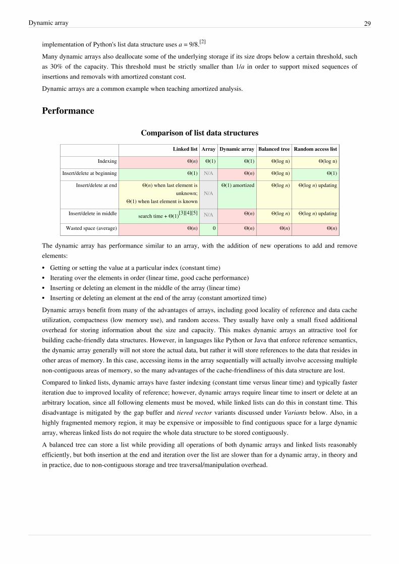
Dynamic array 29

implementation of Python's list data structure uses a = 9/8.[2]

Many dynamic arrays also deallocate some of the underlying storage if its size drops below a certain threshold, suchas 30% of the capacity. This threshold must be strictly smaller than 1/a in order to support mixed sequences ofinsertions and removals with amortized constant cost.Dynamic arrays are a common example when teaching amortized analysis.

Performance

Comparison of list data structures

Linked list Array Dynamic array Balanced tree Random access list

Indexing Θ(n) Θ(1) Θ(1) Θ(log n) Θ(log n)

Insert/delete at beginning Θ(1) N/A Θ(n) Θ(log n) Θ(1)

Insert/delete at end Θ(n) when last element isunknown;

Θ(1) when last element is knownN/A

Θ(1) amortized Θ(log n) Θ(log n) updating

Insert/delete in middle search time + Θ(1)[3][4][5] N/A Θ(n) Θ(log n) Θ(log n) updating

Wasted space (average) Θ(n) 0 Θ(n) Θ(n) Θ(n)

The dynamic array has performance similar to an array, with the addition of new operations to add and removeelements:•• Getting or setting the value at a particular index (constant time)•• Iterating over the elements in order (linear time, good cache performance)•• Inserting or deleting an element in the middle of the array (linear time)•• Inserting or deleting an element at the end of the array (constant amortized time)Dynamic arrays benefit from many of the advantages of arrays, including good locality of reference and data cacheutilization, compactness (low memory use), and random access. They usually have only a small fixed additionaloverhead for storing information about the size and capacity. This makes dynamic arrays an attractive tool forbuilding cache-friendly data structures. However, in languages like Python or Java that enforce reference semantics,the dynamic array generally will not store the actual data, but rather it will store references to the data that resides inother areas of memory. In this case, accessing items in the array sequentially will actually involve accessing multiplenon-contiguous areas of memory, so the many advantages of the cache-friendliness of this data structure are lost.Compared to linked lists, dynamic arrays have faster indexing (constant time versus linear time) and typically fasteriteration due to improved locality of reference; however, dynamic arrays require linear time to insert or delete at anarbitrary location, since all following elements must be moved, while linked lists can do this in constant time. Thisdisadvantage is mitigated by the gap buffer and tiered vector variants discussed under Variants below. Also, in ahighly fragmented memory region, it may be expensive or impossible to find contiguous space for a large dynamicarray, whereas linked lists do not require the whole data structure to be stored contiguously.A balanced tree can store a list while providing all operations of both dynamic arrays and linked lists reasonablyefficiently, but both insertion at the end and iteration over the list are slower than for a dynamic array, in theory andin practice, due to non-contiguous storage and tree traversal/manipulation overhead.

Dynamic array 30

VariantsGap buffers are similar to dynamic arrays but allow efficient insertion and deletion operations clustered near thesame arbitrary location. Some deque implementations use array deques, which allow amortized constant timeinsertion/removal at both ends, instead of just one end.Goodrich presented a dynamic array algorithm called Tiered Vectors that provided O(n1/2) performance for orderpreserving insertions or deletions from the middle of the array.Hashed Array Tree (HAT) is a dynamic array algorithm published by Sitarski in 1996. Hashed Array Tree wastesorder n1/2 amount of storage space, where n is the number of elements in the array. The algorithm has O(1)amortized performance when appending a series of objects to the end of a Hashed Array Tree.In a 1999 paper, Brodnik et al. describe a tiered dynamic array data structure, which wastes only n1/2 space for nelements at any point in time, and they prove a lower bound showing that any dynamic array must waste this muchspace if the operations are to remain amortized constant time. Additionally, they present a variant where growing andshrinking the buffer has not only amortized but worst-case constant time.Bagwell (2002) presented the VList algorithm, which can be adapted to implement a dynamic array.

Language supportC++'s std::vector is an implementation of dynamic arrays, as are the ArrayList[6] classes supplied with theJava API and the .NET Framework. The generic List<> class supplied with version 2.0 of the .NET Framework isalso implemented with dynamic arrays. Smalltalk's OrderedCollection is a dynamic array with dynamic startand end-index, making the removal of the first element also O(1). Python's list datatype implementation is adynamic array. Delphi and D implement dynamic arrays at the language's core. Ada'sAda.Containers.Vectors generic package provides dynamic array implementation for a given subtype. Manyscripting languages such as Perl and Ruby offer dynamic arrays as a built-in primitive data type. Severalcross-platform frameworks provide dynamic array implementations for C: CFArray and CFMutableArray inCore Foundation; GArray and GPtrArray in GLib.

References[1] See, for example, the source code of java.util.ArrayList class from OpenJDK 6 (http:/ / hg. openjdk. java. net/ jdk6/ jdk6/ jdk/ file/

e0e25ac28560/ src/ share/ classes/ java/ util/ ArrayList. java).[2] List object implementation (http:/ / svn. python. org/ projects/ python/ trunk/ Objects/ listobject. c) from python.org, retrieved 2011-09-27.[3] Gerald Kruse. CS 240 Lecture Notes (http:/ / www. juniata. edu/ faculty/ kruse/ cs240/ syllabus. htm): Linked Lists Plus: Complexity

Trade-offs (http:/ / www. juniata. edu/ faculty/ kruse/ cs240/ linkedlist2. htm). Juniata College. Spring 2008.[4] Day 1 Keynote - Bjarne Stroustrup: C++11 Style (http:/ / channel9. msdn. com/ Events/ GoingNative/ GoingNative-2012/

Keynote-Bjarne-Stroustrup-Cpp11-Style) at GoingNative 2012 on channel9.msdn.com from minute 45 or foil 44[5] Number crunching: Why you should never, ever, EVER use linked-list in your code again (http:/ / kjellkod. wordpress. com/ 2012/ 02/ 25/

why-you-should-never-ever-ever-use-linked-list-in-your-code-again/ ) at kjellkod.wordpress.com[6][6] Javadoc on

Dynamic array 31

External links• NIST Dictionary of Algorithms and Data Structures: Dynamic array (http:/ / www. nist. gov/ dads/ HTML/

dynamicarray. html)• VPOOL (http:/ / www. bsdua. org/ libbsdua. html#vpool) - C language implementation of dynamic array.• CollectionSpy (http:/ / www. collectionspy. com) — A Java profiler with explicit support for debugging

ArrayList- and Vector-related issues.• Open Data Structures - Chapter 2 - Array-Based Lists (http:/ / opendatastructures. org/ versions/ edition-0. 1e/

ods-java/ 2_Array_Based_Lists. html)

32

Dictionaries

Associative array"Dictionary (data structure)" redirects here. It is not to be confused with data dictionary.In computer science, an associative array, map, symbol table, or dictionary is an abstract data type composed of acollection of pairs, such that each possible key appears at most once in the collection.Operations associated with this data type allow:•• the addition of pairs to the collection•• the removal of pairs from the collection•• the modification of the values of existing pairs•• the lookup of the value associated with a particular keyThe dictionary problem is a classic computer science problem. The task of designing a data structure that maintainsa set of data during 'search' 'delete' and 'insert' operations. A standard solution to the dictionary problem is a hashtable; in some cases it is also possible to solve the problem using directly addressed arrays, binary search trees, orother more specialized structures.Many programming languages include associative arrays as primitive data types, and they are available in softwarelibraries for many others. Content-addressable memory is a form of direct hardware-level support for associativearrays.Associative arrays have many applications including such fundamental programming patterns as memoization andthe decorator pattern.[1]

OperationsIn an associative array, the association between a key and a value is often known as a "binding", and the same word"binding" may also be used to refer to the process of creating a new association.The operations that are usually defined for an associative array are:

• Add or insert: add a new pair to the collection, binding the new key to its new value. Thearguments to this operation are the key and the value.

• Reassign: replace the value in one of the pairs that are already in the collection, binding an oldkey to a new value. As with an insertion, the arguments to this operation are the key and the value.

• Remove or delete: remove a pair from the collection, unbinding a given key from its value. Theargument to this operation is the key.

• Lookup: find the value (if any) that is bound to a given key. The argument to this operation is the key, and thevalue is returned from the operation. If no value is found, some associative array implementations raise anexception.

In addition, associative arrays may also include other operations such as determining the number of bindings orconstructing an iterator to loop over all the bindings. Usually, for such an operation, the order in which the bindingsare returned may be arbitrary.A multimap generalizes an associative array by allowing multiple values to be associated with a single key.[2] Abidirectional map is a related abstract data type in which the bindings operate in both directions: each value must beassociated with a unique key, and a second lookup operation takes a value as argument and looks up the keyassociated with that value.

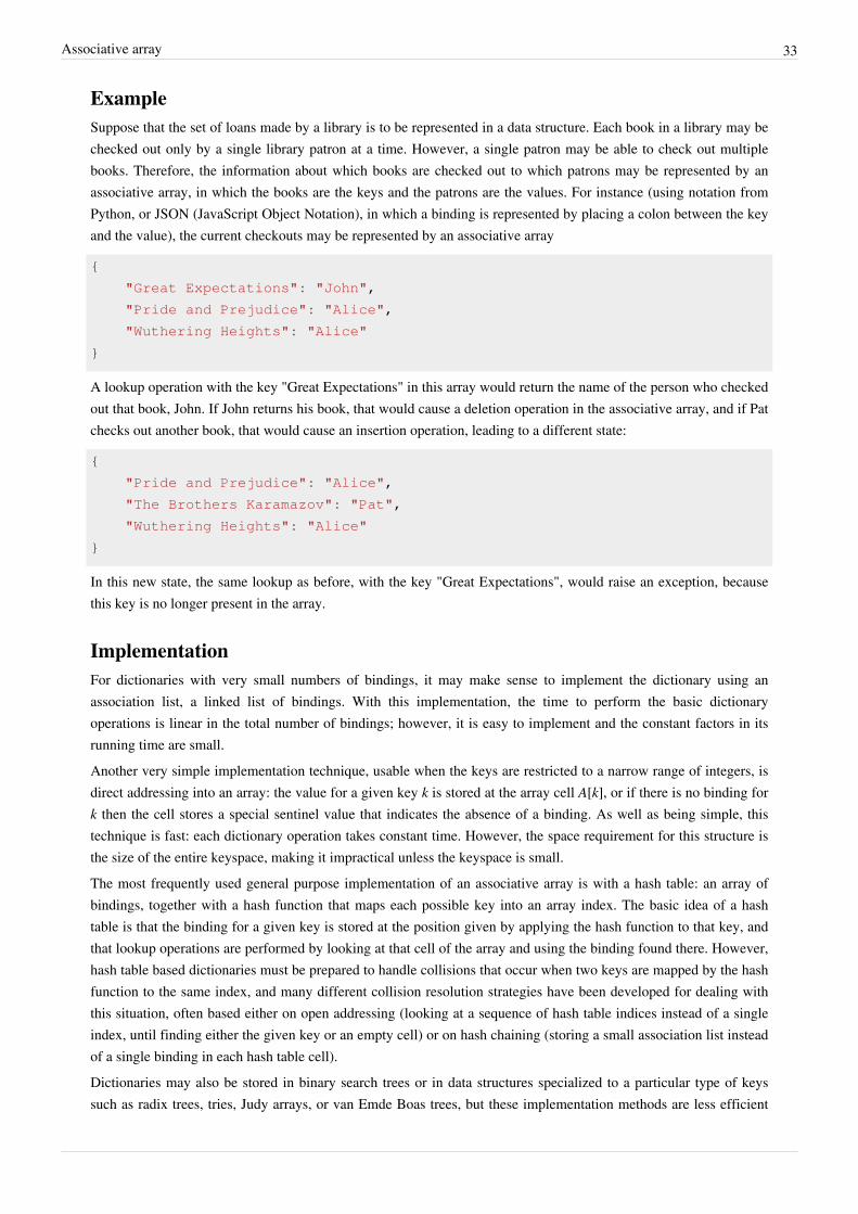
Associative array 33

ExampleSuppose that the set of loans made by a library is to be represented in a data structure. Each book in a library may bechecked out only by a single library patron at a time. However, a single patron may be able to check out multiplebooks. Therefore, the information about which books are checked out to which patrons may be represented by anassociative array, in which the books are the keys and the patrons are the values. For instance (using notation fromPython, or JSON (JavaScript Object Notation), in which a binding is represented by placing a colon between the keyand the value), the current checkouts may be represented by an associative array

{

"Great Expectations": "John",

"Pride and Prejudice": "Alice",

"Wuthering Heights": "Alice"

}

A lookup operation with the key "Great Expectations" in this array would return the name of the person who checkedout that book, John. If John returns his book, that would cause a deletion operation in the associative array, and if Patchecks out another book, that would cause an insertion operation, leading to a different state:

{

"Pride and Prejudice": "Alice",

"The Brothers Karamazov": "Pat",

"Wuthering Heights": "Alice"

}

In this new state, the same lookup as before, with the key "Great Expectations", would raise an exception, becausethis key is no longer present in the array.

ImplementationFor dictionaries with very small numbers of bindings, it may make sense to implement the dictionary using anassociation list, a linked list of bindings. With this implementation, the time to perform the basic dictionaryoperations is linear in the total number of bindings; however, it is easy to implement and the constant factors in itsrunning time are small.Another very simple implementation technique, usable when the keys are restricted to a narrow range of integers, isdirect addressing into an array: the value for a given key k is stored at the array cell A[k], or if there is no binding fork then the cell stores a special sentinel value that indicates the absence of a binding. As well as being simple, thistechnique is fast: each dictionary operation takes constant time. However, the space requirement for this structure isthe size of the entire keyspace, making it impractical unless the keyspace is small.The most frequently used general purpose implementation of an associative array is with a hash table: an array ofbindings, together with a hash function that maps each possible key into an array index. The basic idea of a hashtable is that the binding for a given key is stored at the position given by applying the hash function to that key, andthat lookup operations are performed by looking at that cell of the array and using the binding found there. However,hash table based dictionaries must be prepared to handle collisions that occur when two keys are mapped by the hashfunction to the same index, and many different collision resolution strategies have been developed for dealing withthis situation, often based either on open addressing (looking at a sequence of hash table indices instead of a singleindex, until finding either the given key or an empty cell) or on hash chaining (storing a small association list insteadof a single binding in each hash table cell).Dictionaries may also be stored in binary search trees or in data structures specialized to a particular type of keys such as radix trees, tries, Judy arrays, or van Emde Boas trees, but these implementation methods are less efficient

Associative array 34

than hash tables as well as placing greater restrictions on the types of data that they can handle. The advantages ofthese alternative structures come from their ability to handle operations beyond the basic ones of an associativearray, such as finding the binding whose key is the closest to a queried key, when the query is not itself present in theset of bindings.

Language supportMain article: Comparison of programming languages (mapping)Associative arrays can be implemented in any programming language as a package and many language systemsprovide them as part of their standard library. In some languages, they are not only built into the standard system, buthave special syntax, often using array-like subscripting.Built-in syntactic support for associative arrays was introduced by SNOBOL4, under the name "table". MUMPSmade multi-dimensional associative arrays, optionally persistent, its key data structure. SETL supported them as onepossible implementation of sets and maps. Most modern scripting languages, starting with AWK and includingRexx, Perl, Tcl, JavaScript, Python, Ruby, and Lua, support associative arrays as a primary container type. In manymore languages, they are available as library functions without special syntax.In Smalltalk, Objective-C, .NET, Python, REALbasic, and Swift they are called dictionaries; in Perl, Ruby andSeed7 they are called hashes; in C++, Java, Go, Clojure, Scala, OCaml, Haskell they are called maps (see map(C++), unordered_map (C++), and Map [3]); in Common Lisp and Windows PowerShell, they are called hash tables(since both typically use this implementation). In PHP, all arrays can be associative, except that the keys are limitedto integers and strings. In JavaScript (see also JSON), all objects behave as associative arrays. In Lua, they are calledtables, and are used as the primitive building block for all data structures. In Visual FoxPro, they are calledCollections.

References[1] , pp. 597–599.[2] , pp. 389–397.[3] http:/ / docs. oracle. com/ javase/ 7/ docs/ api/ java/ util/ Map. html

External links

Look up associative array in Wiktionary, the free dictionary.

• NIST's Dictionary of Algorithms and Data Structures: Associative Array (http:/ / www. nist. gov/ dads/ HTML/assocarray. html)

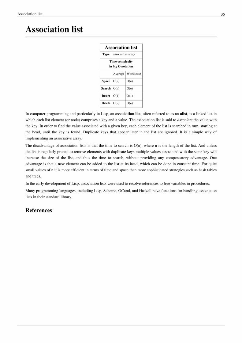
Association list 35

Association list

Association listType associative array

Time complexityin big O notation

Average Worst case

Space O(n) O(n)

Search O(n) O(n)

Insert O(1) O(1)

Delete O(n) O(n)

In computer programming and particularly in Lisp, an association list, often referred to as an alist, is a linked list inwhich each list element (or node) comprises a key and a value. The association list is said to associate the value withthe key. In order to find the value associated with a given key, each element of the list is searched in turn, starting atthe head, until the key is found. Duplicate keys that appear later in the list are ignored. It is a simple way ofimplementing an associative array.The disadvantage of association lists is that the time to search is O(n), where n is the length of the list. And unlessthe list is regularly pruned to remove elements with duplicate keys multiple values associated with the same key willincrease the size of the list, and thus the time to search, without providing any compensatory advantage. Oneadvantage is that a new element can be added to the list at its head, which can be done in constant time. For quitesmall values of n it is more efficient in terms of time and space than more sophisticated strategies such as hash tablesand trees.In the early development of Lisp, association lists were used to resolve references to free variables in procedures.Many programming languages, including Lisp, Scheme, OCaml, and Haskell have functions for handling associationlists in their standard library.

References

Hash table 36

Hash tableNot to be confused with Hash list or Hash tree.

Hash tableType Unordered associative array

Invented 1953

Time complexityin big O notation

Average Worst case

Space O(n) O(n)

Search O(1) O(n)

Insert O(1) O(n)

Delete O(1) O(n)

A small phone book as a hash table

In computing, a hash table (also hashmap) is a data structure used toimplement an associative array, astructure that can map keys to values. Ahash table uses a hash function tocompute an index into an array ofbuckets or slots, from which the correctvalue can be found.

Ideally, the hash function will assigneach key to a unique bucket, but thissituation is rarely achievable in practice(usually some keys will hash to the samebucket). Instead, most hash table designsassume that hash collisions—differentkeys that are assigned by the hashfunction to the same bucket—will occurand must be accommodated in some way.

In a well-dimensioned hash table, the average cost (number of instructions) for each lookup is independent of thenumber of elements stored in the table. Many hash table designs also allow arbitrary insertions and deletions ofkey-value pairs, at (amortized[1]) constant average cost per operation.

In many situations, hash tables turn out to be more efficient than search trees or any other table lookup structure. Forthis reason, they are widely used in many kinds of computer software, particularly for associative arrays, databaseindexing, caches, and sets.

Hash table 37

HashingMain article: Hash functionThe idea of hashing is to distribute the entries (key/value pairs) across an array of buckets. Given a key, thealgorithm computes an index that suggests where the entry can be found:

index = f(key, array_size)

Often this is done in two steps:

hash = hashfunc(key)

index = hash % array_size

In this method, the hash is independent of the array size, and it is then reduced to an index (a number between 0 andarray_size − 1) using the modulo operator (%).In the case that the array size is a power of two, the remainder operation is reduced to masking, which improvesspeed, but can increase problems with a poor hash function.

Choosing a good hash functionA good hash function and implementation algorithm are essential for good hash table performance, but may bedifficult to achieve.A basic requirement is that the function should provide a uniform distribution of hash values. A non-uniformdistribution increases the number of collisions and the cost of resolving them. Uniformity is sometimes difficult toensure by design, but may be evaluated empirically using statistical tests, e.g. a Pearson's chi-squared test for discreteuniform distributions.The distribution needs to be uniform only for table sizes that occur in the application. In particular, if one usesdynamic resizing with exact doubling and halving of the table size s, then the hash function needs to be uniform onlywhen s is a power of two. On the other hand, some hashing algorithms provide uniform hashes only when s is aprime number.[2]

For open addressing schemes, the hash function should also avoid clustering, the mapping of two or more keys toconsecutive slots. Such clustering may cause the lookup cost to skyrocket, even if the load factor is low andcollisions are infrequent. The popular multiplicative hash is claimed to have particularly poor clustering behavior.Cryptographic hash functions are believed to provide good hash functions for any table size s, either by moduloreduction or by bit maskingWikipedia:Citation needed. They may also be appropriate if there is a risk of malicioususers trying to sabotage a network service by submitting requests designed to generate a large number of collisionsin the server's hash tables. However, the risk of sabotage can also be avoided by cheaper methods (such as applying asecret salt to the data, or using a universal hash function).

Perfect hash functionIf all keys are known ahead of time, a perfect hash function can be used to create a perfect hash table that has nocollisions. If minimal perfect hashing is used, every location in the hash table can be used as well.Perfect hashing allows for constant time lookups in the worst case. This is in contrast to most chaining and openaddressing methods, where the time for lookup is low on average, but may be very large (proportional to the numberof entries) for some sets of keys.

Hash table 38

Key statisticsA critical statistic for a hash table is called the load factor. This is simply the number of entries divided by thenumber of buckets, that is, n/k where n is the number of entries and k is the number of buckets.If the load factor is kept reasonable, the hash table should perform well, provided the hashing is good. If the loadfactor grows too large, the hash table will become slow, or it may fail to work (depending on the method used). Theexpected constant time property of a hash table assumes that the load factor is kept below some bound. For a fixednumber of buckets, the time for a lookup grows with the number of entries and so does not achieve the desiredconstant time.Second to that, one can examine the variance of number of entries per bucket. For example, two tables both have1000 entries and 1000 buckets; one has exactly one entry in each bucket, the other has all entries in the same bucket.Clearly the hashing is not working in the second one.A low load factor is not especially beneficial. As the load factor approaches 0, the proportion of unused areas in thehash table increases, but there is not necessarily any reduction in search cost. This results in wasted memory.

Collision resolutionHash collisions are practically unavoidable when hashing a random subset of a large set of possible keys. Forexample, if 2,450 keys are hashed into a million buckets, even with a perfectly uniform random distribution,according to the birthday problem there is approximately a 95% chance of at least two of the keys being hashed tothe same slot.Therefore, most hash table implementations have some collision resolution strategy to handle such events. Somecommon strategies are described below. All these methods require that the keys (or pointers to them) be stored in thetable, together with the associated values.

Separate chaining

Hash collision resolved by separate chaining.

In the method known as separatechaining, each bucket is independent,and has some sort of list of entries withthe same index. The time for hash tableoperations is the time to find thebucket (which is constant) plus thetime for the list operation. (Thetechnique is also called open hashingor closed addressing.)

In a good hash table, each bucket haszero or one entries, and sometimes twoor three, but rarely more than that.Therefore, structures that are efficientin time and space for these cases arepreferred. Structures that are efficientfor a fairly large number of entries arenot needed or desirable. If these cases happen often, the hashing is not working well, and this needs to be fixed.

Hash table 39

Separate chaining with linked lists

Chained hash tables with linked lists are popular because they require only basic data structures with simplealgorithms, and can use simple hash functions that are unsuitable for other methods.The cost of a table operation is that of scanning the entries of the selected bucket for the desired key. If thedistribution of keys is sufficiently uniform, the average cost of a lookup depends only on the average number of keysper bucket—that is, on the load factor.Chained hash tables remain effective even when the number of table entries n is much higher than the number ofslots. Their performance degrades more gracefully (linearly) with the load factor. For example, a chained hash tablewith 1000 slots and 10,000 stored keys (load factor 10) is five to ten times slower than a 10,000-slot table (loadfactor 1); but still 1000 times faster than a plain sequential list, and possibly even faster than a balanced searchtree.Wikipedia:Citation neededFor separate-chaining, the worst-case scenario is when all entries are inserted into the same bucket, in which case thehash table is ineffective and the cost is that of searching the bucket data structure. If the latter is a linear list, thelookup procedure may have to scan all its entries, so the worst-case cost is proportional to the number n of entries inthe table.The bucket chains are often implemented as ordered lists, sorted by the key field; this choice approximately halvesthe average cost of unsuccessful lookups, compared to an unordered listWikipedia:Citation needed. However, ifsome keys are much more likely to come up than others, an unordered list with move-to-front heuristic may be moreeffective. More sophisticated data structures, such as balanced search trees, are worth considering only if the loadfactor is large (about 10 or more), or if the hash distribution is likely to be very non-uniform, or if one mustguarantee good performance even in a worst-case scenario. However, using a larger table and/or a better hashfunction may be even more effective in those cases.Chained hash tables also inherit the disadvantages of linked lists. When storing small keys and values, the spaceoverhead of the next pointer in each entry record can be significant. An additional disadvantage is that traversing alinked list has poor cache performance, making the processor cache ineffective.

Separate chaining with list head cells

Hash collision by separate chaining with head records in the bucket array.

Some chaining implementations storethe first record of each chain in the slotarray itself. The number of pointertraversals is decreased by one for mostcases. The purpose is to increase cacheefficiency of hash table access.The disadvantage is that an emptybucket takes the same space as abucket with one entry. To save space,such hash tables often have about asmany slots as stored entries, meaningthat many slots have two or moreentries.

Hash table 40

Separate chaining with other structures

Instead of a list, one can use any other data structure that supports the required operations. For example, by using aself-balancing tree, the theoretical worst-case time of common hash table operations (insertion, deletion, lookup) canbe brought down to O(log n) rather than O(n). However, this approach is only worth the trouble and extra memorycost if long delays must be avoided at all costs (e.g. in a real-time application), or if one must guard against manyentries hashed to the same slot (e.g. if one expects extremely non-uniform distributions, or in the case of web sites orother publicly accessible services, which are vulnerable to malicious key distributions in requests).The variant called array hash table uses a dynamic array to store all the entries that hash to the same slot. Each newlyinserted entry gets appended to the end of the dynamic array that is assigned to the slot. The dynamic array is resizedin an exact-fit manner, meaning it is grown only by as many bytes as needed. Alternative techniques such as growingthe array by block sizes or pages were found to improve insertion performance, but at a cost in space. This variationmakes more efficient use of CPU caching and the translation lookaside buffer (TLB), because slot entries are storedin sequential memory positions. It also dispenses with the next pointers that are required by linked lists, whichsaves space. Despite frequent array resizing, space overheads incurred by operating system such as memoryfragmentation, were found to be small.An elaboration on this approach is the so-called dynamic perfect hashing,[3] where a bucket that contains k entries isorganized as a perfect hash table with k2 slots. While it uses more memory (n2 slots for n entries, in the worst caseand n*k slots in the average case), this variant has guaranteed constant worst-case lookup time, and low amortizedtime for insertion.

Open addressing

Hash collision resolved by open addressing with linear probing (interval=1). Note that"Ted Baker" has a unique hash, but nevertheless collided with "Sandra Dee", that had

previously collided with "John Smith".

In another strategy, called openaddressing, all entry records are storedin the bucket array itself. When a newentry has to be inserted, the buckets areexamined, starting with the hashed-toslot and proceeding in some probesequence, until an unoccupied slot isfound. When searching for an entry,the buckets are scanned in the samesequence, until either the target recordis found, or an unused array slot isfound, which indicates that there is nosuch key in the table. The name "openaddressing" refers to the fact that thelocation ("address") of the item is notdetermined by its hash value. (Thismethod is also called closed hashing;it should not be confused with "openhashing" or "closed addressing" thatusually mean separate chaining.)

Well-known probe sequences include:• Linear probing, in which the interval between probes is fixed (usually 1)• Quadratic probing, in which the interval between probes is increased by adding the successive outputs of a

quadratic polynomial to the starting value given by the original hash computation

Hash table 41

• Double hashing, in which the interval between probes is computed by another hash functionA drawback of all these open addressing schemes is that the number of stored entries cannot exceed the number ofslots in the bucket array. In fact, even with good hash functions, their performance dramatically degrades when theload factor grows beyond 0.7 or so. Thus a more aggressive resize scheme is needed. Separate linking workscorrectly with any load factor, although performance is likely to be reasonable if it is kept below 2 or so. For manyapplications, these restrictions mandate the use of dynamic resizing, with its attendant costs.Open addressing schemes also put more stringent requirements on the hash function: besides distributing the keysmore uniformly over the buckets, the function must also minimize the clustering of hash values that are consecutivein the probe order. Using separate chaining, the only concern is that too many objects map to the same hash value;whether they are adjacent or nearby is completely irrelevant.Open addressing only saves memory if the entries are small (less than four times the size of a pointer) and the loadfactor is not too small. If the load factor is close to zero (that is, there are far more buckets than stored entries), openaddressing is wasteful even if each entry is just two words.

This graph compares the average number of cache misses required to look up elements intables with chaining and linear probing. As the table passes the 80%-full mark, linear

probing's performance drastically degrades.

Open addressing avoids the timeoverhead of allocating each new entryrecord, and can be implemented evenin the absence of a memory allocator.It also avoids the extra indirectionrequired to access the first entry ofeach bucket (that is, usually the onlyone). It also has better locality ofreference, particularly with linearprobing. With small record sizes, thesefactors can yield better performancethan chaining, particularly for lookups.Hash tables with open addressing arealso easier to serialize, because they donot use pointers.

On the other hand, normal openaddressing is a poor choice for large elements, because these elements fill entire CPU cache lines (negating the cacheadvantage), and a large amount of space is wasted on large empty table slots. If the open addressing table only storesreferences to elements (external storage), it uses space comparable to chaining even for large records but loses itsspeed advantage.

Generally speaking, open addressing is better used for hash tables with small records that can be stored within thetable (internal storage) and fit in a cache line. They are particularly suitable for elements of one word or less. If thetable is expected to have a high load factor, the records are large, or the data is variable-sized, chained hash tablesoften perform as well or better.Ultimately, used sensibly, any kind of hash table algorithm is usually fast enough; and the percentage of acalculation spent in hash table code is low. Memory usage is rarely considered excessive. Therefore, in most casesthe differences between these algorithms are marginal, and other considerations typically come intoplay.Wikipedia:Citation needed

Hash table 42

Coalesced hashingA hybrid of chaining and open addressing, coalesced hashing links together chains of nodes within the table itself.Like open addressing, it achieves space usage and (somewhat diminished) cache advantages over chaining. Likechaining, it does not exhibit clustering effects; in fact, the table can be efficiently filled to a high density. Unlikechaining, it cannot have more elements than table slots.

Cuckoo hashingAnother alternative open-addressing solution is cuckoo hashing, which ensures constant lookup time in the worstcase, and constant amortized time for insertions and deletions. It uses two or more hash functions, which means anykey/value pair could be in two or more locations. For lookup, the first hash function is used; if the key/value is notfound, then the second hash function is used, and so on. If a collision happens during insertion, then the key isre-hashed with the second hash function to map it to another bucket. If all hash functions are used and there is still acollision, then the key it collided with is removed to make space for the new key, and the old key is re-hashed withone of the other hash functions, which maps it to another bucket. If that location also results in a collision, then theprocess repeats until there is no collision or the process traverses all the buckets, at which point the table is resized.By combining multiple hash functions with multiple cells per bucket, very high space utilisation can be achieved.

Robin Hood hashingOne interesting variation on double-hashing collision resolution is Robin Hood hashing. The idea is that a new keymay displace a key already inserted, if its probe count is larger than that of the key at the current position. The neteffect of this is that it reduces worst case search times in the table. This is similar to ordered hash tables except thatthe criterion for bumping a key does not depend on a direct relationship between the keys. Since both the worst caseand the variation in the number of probes is reduced dramatically, an interesting variation is to probe the tablestarting at the expected successful probe value and then expand from that position in both directions. External RobinHashing is an extension of this algorithm where the table is stored in an external file and each table positioncorresponds to a fixed-sized page or bucket with B records.

2-choice hashing2-choice hashing employs 2 different hash functions, h1(x) and h2(x), for the hash table. Both hash functions are usedto compute two table locations. When an object is inserted in the table, then it is placed in the table location thatcontains fewer objects (with the default being the h1(x) table location if there is equality in bucket size). 2-choicehashing employs the principle of the power of two choices.

Hopscotch hashingAnother alternative open-addressing solution is hopscotch hashing, which combines the approaches of cuckoohashing and linear probing, yet seems in general to avoid their limitations. In particular it works well even when theload factor grows beyond 0.9. The algorithm is well suited for implementing a resizable concurrent hash table.The hopscotch hashing algorithm works by defining a neighborhood of buckets near the original hashed bucket,where a given entry is always found. Thus, search is limited to the number of entries in this neighborhood, which islogarithmic in the worst case, constant on average, and with proper alignment of the neighborhood typically requiresone cache miss. When inserting an entry, one first attempts to add it to a bucket in the neighborhood. However, if allbuckets in this neighborhood are occupied, the algorithm traverses buckets in sequence until an open slot (anunoccupied bucket) is found (as in linear probing). At that point, since the empty bucket is outside the neighborhood,items are repeatedly displaced in a sequence of hops. (This is similar to cuckoo hashing, but with the difference thatin this case the empty slot is being moved into the neighborhood, instead of items being moved out with the hope ofeventually finding an empty slot.) Each hop brings the open slot closer to the original neighborhood, without

Hash table 43

invalidating the neighborhood property of any of the buckets along the way. In the end, the open slot has beenmoved into the neighborhood, and the entry being inserted can be added to it.

Dynamic resizingThe good functioning of a hash table depends on the fact that the table size is proportional to the number of entries.With a fixed size, and the common structures, it is similar to linear search, except with a better constant factor. Insome cases, the number of entries may be definitely known in advance, for example keywords in a language. Morecommonly, this is not known for sure, if only due to later changes in code and data. It is one serious, althoughcommon, mistake to not provide any way for the table to resize. A general-purpose hash table "class" will almostalways have some way to resize, and it is good practice even for simple "custom" tables. An implementation shouldcheck the load factor, and do something if it becomes too large (this needs to be done only on inserts, since that is theonly thing that would increase it).To keep the load factor under a certain limit, e.g. under 3/4, many table implementations expand the table whenitems are inserted. For example, in Java's HashMap class the default load factor threshold for table expansion is0.75 and in Python's dict, table size is resized when load factor is greater than 2/3.Since buckets are usually implemented on top of a dynamic array and any constant proportion for resizing greaterthan 1 will keep the load factor under the desired limit, the exact choice of the constant is determined by the samespace-time tradeoff as for dynamic arrays.Resizing is accompanied by a full or incremental table rehash whereby existing items are mapped to new bucketlocations.To limit the proportion of memory wasted due to empty buckets, some implementations also shrink the size of thetable—followed by a rehash—when items are deleted. From the point of space-time tradeoffs, this operation issimilar to the deallocation in dynamic arrays.

Resizing by copying all entriesA common approach is to automatically trigger a complete resizing when the load factor exceeds some thresholdrmax. Then a new larger table is allocated, all the entries of the old table are removed and inserted into this new table,and the old table is returned to the free storage pool. Symmetrically, when the load factor falls below a secondthreshold rmin, all entries are moved to a new smaller table.If the table size increases or decreases by a fixed percentage at each expansion, the total cost of these resizings,amortized over all insert and delete operations, is still a constant, independent of the number of entries n and of thenumber m of operations performed.For example, consider a table that was created with the minimum possible size and is doubled each time the loadratio exceeds some threshold. If m elements are inserted into that table, the total number of extra re-insertions thatoccur in all dynamic resizings of the table is at most m − 1. In other words, dynamic resizing roughly doubles thecost of each insert or delete operation.

Hash table 44

Incremental resizingSome hash table implementations, notably in real-time systems, cannot pay the price of enlarging the hash table all atonce, because it may interrupt time-critical operations. If one cannot avoid dynamic resizing, a solution is to performthe resizing gradually:•• During the resize, allocate the new hash table, but keep the old table unchanged.•• In each lookup or delete operation, check both tables.•• Perform insertion operations only in the new table.• At each insertion also move r elements from the old table to the new table.•• When all elements are removed from the old table, deallocate it.To ensure that the old table is completely copied over before the new table itself needs to be enlarged, it is necessaryto increase the size of the table by a factor of at least (r + 1)/r during resizing.

Monotonic keysIf it is known that key values will always increase (or decrease) monotonically, then a variation of consistent hashingcan be achieved by keeping a list of the single most recent key value at each hash table resize operation. Uponlookup, keys that fall in the ranges defined by these list entries are directed to the appropriate hash function—andindeed hash table—both of which can be different for each range. Since it is common to grow the overall number ofentries by doubling, there will only be O(lg(N)) ranges to check, and binary search time for the redirection would beO(lg(lg(N))). As with consistent hashing, this approach guarantees that any key's hash, once issued, will neverchange, even when the hash table is later grown.

Other solutionsLinear hashing is a hash table algorithm that permits incremental hash table expansion. It is implemented using asingle hash table, but with two possible look-up functions.Another way to decrease the cost of table resizing is to choose a hash function in such a way that the hashes of mostvalues do not change when the table is resized. This approach, called consistent hashing, is prevalent in disk-basedand distributed hashes, where rehashing is prohibitively costly.

Performance analysisIn the simplest model, the hash function is completely unspecified and the table does not resize. For the best possiblechoice of hash function, a table of size k with open addressing has no collisions and holds up to k elements, with asingle comparison for successful lookup, and a table of size k with chaining and n keys has the minimum max(0, n-k)collisions and O(1 + n/k) comparisons for lookup. For the worst choice of hash function, every insertion causes acollision, and hash tables degenerate to linear search, with Ω(n) amortized comparisons per insertion and up to ncomparisons for a successful lookup.Adding rehashing to this model is straightforward. As in a dynamic array, geometric resizing by a factor of b impliesthat only n/bi keys are inserted i or more times, so that the total number of insertions is bounded above by bn/(b-1),which is O(n). By using rehashing to maintain n < k, tables using both chaining and open addressing can haveunlimited elements and perform successful lookup in a single comparison for the best choice of hash function.In more realistic models, the hash function is a random variable over a probability distribution of hash functions, andperformance is computed on average over the choice of hash function. When this distribution is uniform, theassumption is called "simple uniform hashing" and it can be shown that hashing with chaining requires Θ(1 + n/k)comparisons on average for an unsuccessful lookup, and hashing with open addressing requires Θ(1/(1 - n/k)).[4]

Both these bounds are constant, if we maintain n/k < c using table resizing, where c is a fixed constant less than 1.

Hash table 45

Features

AdvantagesThe main advantage of hash tables over other table data structures is speed. This advantage is more apparent whenthe number of entries is large. Hash tables are particularly efficient when the maximum number of entries can bepredicted in advance, so that the bucket array can be allocated once with the optimum size and never resized.If the set of key-value pairs is fixed and known ahead of time (so insertions and deletions are not allowed), one mayreduce the average lookup cost by a careful choice of the hash function, bucket table size, and internal datastructures. In particular, one may be able to devise a hash function that is collision-free, or even perfect (see below).In this case the keys need not be stored in the table.

DrawbacksAlthough operations on a hash table take constant time on average, the cost of a good hash function can besignificantly higher than the inner loop of the lookup algorithm for a sequential list or search tree. Thus hash tablesare not effective when the number of entries is very small. (However, in some cases the high cost of computing thehash function can be mitigated by saving the hash value together with the key.)For certain string processing applications, such as spell-checking, hash tables may be less efficient than tries, finiteautomata, or Judy arrays. Also, if each key is represented by a small enough number of bits, then, instead of a hashtable, one may use the key directly as the index into an array of values. Note that there are no collisions in this case.The entries stored in a hash table can be enumerated efficiently (at constant cost per entry), but only in somepseudo-random order. Therefore, there is no efficient way to locate an entry whose key is nearest to a given key.Listing all n entries in some specific order generally requires a separate sorting step, whose cost is proportional tolog(n) per entry. In comparison, ordered search trees have lookup and insertion cost proportional to log(n), but allowfinding the nearest key at about the same cost, and ordered enumeration of all entries at constant cost per entry.If the keys are not stored (because the hash function is collision-free), there may be no easy way to enumerate thekeys that are present in the table at any given moment.Although the average cost per operation is constant and fairly small, the cost of a single operation may be quite high.In particular, if the hash table uses dynamic resizing, an insertion or deletion operation may occasionally take timeproportional to the number of entries. This may be a serious drawback in real-time or interactive applications.Hash tables in general exhibit poor locality of reference—that is, the data to be accessed is distributed seemingly atrandom in memory. Because hash tables cause access patterns that jump around, this can trigger microprocessorcache misses that cause long delays. Compact data structures such as arrays searched with linear search may befaster, if the table is relatively small and keys are compact. The optimal performance point varies from system tosystem.Hash tables become quite inefficient when there are many collisions. While extremely uneven hash distributions areextremely unlikely to arise by chance, a malicious adversary with knowledge of the hash function may be able tosupply information to a hash that creates worst-case behavior by causing excessive collisions, resulting in very poorperformance, e.g. a denial of service attack.[5] In critical applications, universal hashing can be used; a data structurewith better worst-case guarantees may be preferable.[6]

Hash table 46

Uses

Associative arraysHash tables are commonly used to implement many types of in-memory tables. They are used to implementassociative arrays (arrays whose indices are arbitrary strings or other complicated objects), especially in interpretedprogramming languages like AWK, Perl, and PHP.When storing a new item into a multimap and a hash collision occurs, the multimap unconditionally stores bothitems.When storing a new item into a typical associative array and a hash collision occurs, but the actual keys themselvesare different, the associative array likewise stores both items. However, if the key of the new item exactly matchesthe key of an old item, the associative array typically erases the old item and overwrites it with the new item, soevery item in the table has a unique key.

Database indexingHash tables may also be used as disk-based data structures and database indices (such as in dbm) although B-treesare more popular in these applications.

CachesHash tables can be used to implement caches, auxiliary data tables that are used to speed up the access to data that isprimarily stored in slower media. In this application, hash collisions can be handled by discarding one of the twocolliding entries—usually erasing the old item that is currently stored in the table and overwriting it with the newitem, so every item in the table has a unique hash value.

SetsBesides recovering the entry that has a given key, many hash table implementations can also tell whether such anentry exists or not.Those structures can therefore be used to implement a set data structure, which merely records whether a given keybelongs to a specified set of keys. In this case, the structure can be simplified by eliminating all parts that have to dowith the entry values. Hashing can be used to implement both static and dynamic sets.

Object representationSeveral dynamic languages, such as Perl, Python, JavaScript, and Ruby, use hash tables to implement objects. In thisrepresentation, the keys are the names of the members and methods of the object, and the values are pointers to thecorresponding member or method.

Unique data representationHash tables can be used by some programs to avoid creating multiple character strings with the same contents. Forthat purpose, all strings in use by the program are stored in a single string pool implemented as a hash table, which ischecked whenever a new string has to be created. This technique was introduced in Lisp interpreters under the namehash consing, and can be used with many other kinds of data (expression trees in a symbolic algebra system, recordsin a database, files in a file system, binary decision diagrams, etc.)

Hash table 47

String interningMain article: String interning

Implementations

In programming languagesMany programming languages provide hash table functionality, either as built-in associative arrays or as standardlibrary modules. In C++11, for example, the unordered_map class provides hash tables for keys and values ofarbitrary type.In PHP 5, the Zend 2 engine uses one of the hash functions from Daniel J. Bernstein to generate the hash values usedin managing the mappings of data pointers stored in a hash table. In the PHP source code, it is labelled as DJBX33A(Daniel J. Bernstein, Times 33 with Addition).Python's built-in hash table implementation, in the form of the dict type, as well as Perl's hash type (%) are usedinternally to implement namespaces and therefore need to pay more attention to security, i.e. collision attacks.In the .NET Framework, support for hash tables is provided via the non-generic Hashtable and genericDictionary classes, which store key-value pairs, and the generic HashSet class, which stores only values.

Independent packages• SparseHash [7] (formerly Google SparseHash) An extremely memory-efficient hash_map implementation, with

only 2 bits/entry of overhead. The SparseHash library has several C++ hash map implementations with differentperformance characteristics, including one that optimizes for memory use and another that optimizes for speed.

• SunriseDD [8] An open source C library for hash table storage of arbitrary data objects with lock-free lookups,built-in reference counting and guaranteed order iteration. The library can participate in external referencecounting systems or use its own built-in reference counting. It comes with a variety of hash functions and allowsthe use of runtime supplied hash functions via callback mechanism. Source code is well documented.

• uthash [9] This is an easy-to-use hash table for C structures.

HistoryThe idea of hashing arose independently in different places. In January 1953, H. P. Luhn wrote an internal IBMmemorandum that used hashing with chaining. G. N. Amdahl, E. M. Boehme, N. Rochester, and Arthur Samuelimplemented a program using hashing at about the same time. Open addressing with linear probing (relatively primestepping) is credited to Amdahl, but Ershov (in Russia) had the same idea.

References[1] Charles E. Leiserson, Amortized Algorithms, Table Doubling, Potential Method (http:/ / videolectures. net/ mit6046jf05_leiserson_lec13/ )

Lecture 13, course MIT 6.046J/18.410J Introduction to Algorithms—Fall 2005[2] Thomas Wang (1997), Prime Double Hash Table (http:/ / www. concentric. net/ ~Ttwang/ tech/ primehash. htm). Retrieved April 27, 2012[3] Erik Demaine, Jeff Lind. 6.897: Advanced Data Structures. MIT Computer Science and Artificial Intelligence Laboratory. Spring 2003. http:/

/ courses. csail. mit. edu/ 6. 897/ spring03/ scribe_notes/ L2/ lecture2. pdf[4] Doug Dunham. CS 4521 Lecture Notes (http:/ / www. duluth. umn. edu/ ~ddunham/ cs4521s09/ notes/ ch11. txt). University of Minnesota

Duluth. Theorems 11.2, 11.6. Last modified April 21, 2009.[5] Alexander Klink and Julian Wälde's Efficient Denial of Service Attacks on Web Application Platforms (http:/ / events. ccc. de/ congress/

2011/ Fahrplan/ attachments/ 2007_28C3_Effective_DoS_on_web_application_platforms. pdf), December 28, 2011, 28th ChaosCommunication Congress. Berlin, Germany.

[6] Crosby and Wallach's Denial of Service via Algorithmic Complexity Attacks (http:/ / www. cs. rice. edu/ ~scrosby/ hash/CrosbyWallach_UsenixSec2003. pdf).

[7] http:/ / code. google. com/ p/ sparsehash/

Hash table 48

[8] http:/ / www. sunrisetel. net/ software/ devtools/ sunrise-data-dictionary. shtml[9] http:/ / uthash. sourceforge. net/

Further reading• Tamassia, Roberto; Goodrich, Michael T. (2006). "Chapter Nine: Maps and Dictionaries". Data structures and

algorithms in Java : [updated for Java 5.0] (4th ed.). Hoboken, NJ: Wiley. pp. 369–418. ISBN 0-471-73884-0.• McKenzie, B. J.; Harries, R.; Bell, T. (Feb 1990). "Selecting a hashing algorithm". Software Practice &

Experience 20 (2): 209–224. doi: 10.1002/spe.4380200207 (http:/ / dx. doi. org/ 10. 1002/ spe. 4380200207).

External links

Wikimedia Commons has media related to Hash tables.

• A Hash Function for Hash Table Lookup (http:/ / www. burtleburtle. net/ bob/ hash/ doobs. html) by Bob Jenkins.• Hash Tables (http:/ / www. sparknotes. com/ cs/ searching/ hashtables/ summary. html) by

SparkNotes—explanation using C• Hash functions (http:/ / www. azillionmonkeys. com/ qed/ hash. html) by Paul Hsieh• Design of Compact and Efficient Hash Tables for Java (http:/ / blog. griddynamics. com/ 2011/ 03/

ultimate-sets-and-maps-for-java-part-i. html) link not working• Libhashish (http:/ / libhashish. sourceforge. net/ ) hash library• NIST entry on hash tables (http:/ / www. nist. gov/ dads/ HTML/ hashtab. html)• Open addressing hash table removal algorithm from ICI programming language, ici_set_unassign in set.c (http:/ /

ici. cvs. sourceforge. net/ ici/ ici/ set. c?view=markup) (and other occurrences, with permission).• A basic explanation of how the hash table works by Reliable Software (http:/ / www. relisoft. com/ book/ lang/

pointer/ 8hash. html)• Lecture on Hash Tables (http:/ / compgeom. cs. uiuc. edu/ ~jeffe/ teaching/ 373/ notes/ 06-hashing. pdf)• Hash-tables in C (http:/ / task3. cc/ 308/ hash-maps-with-linear-probing-and-separate-chaining/ )—two simple and

clear examples of hash tables implementation in C with linear probing and chaining• Open Data Structures - Chapter 5 - Hash Tables (http:/ / opendatastructures. org/ versions/ edition-0. 1e/ ods-java/

5_Hash_Tables. html)• MIT's Introduction to Algorithms: Hashing 1 (http:/ / ocw. mit. edu/ courses/

electrical-engineering-and-computer-science/ 6-046j-introduction-to-algorithms-sma-5503-fall-2005/video-lectures/ lecture-7-hashing-hash-functions/ ) MIT OCW lecture Video

• MIT's Introduction to Algorithms: Hashing 2 (http:/ / ocw. mit. edu/ courses/electrical-engineering-and-computer-science/ 6-046j-introduction-to-algorithms-sma-5503-fall-2005/video-lectures/ lecture-8-universal-hashing-perfect-hashing/ ) MIT OCW lecture Video

• How to sort a HashMap (Java) and keep the duplicate entries (http:/ / www. lampos. net/ sort-hashmap)• How python dictionary works (http:/ / www. laurentluce. com/ posts/ python-dictionary-implementation/ )

Linear probing 49

Linear probingLinear probing is a scheme in computer programming for resolving hash collisions of values of hash functions bysequentially searching the hash table for a free location.

AlgorithmLinear probing is accomplished using two values - one as a starting value and one as an interval between successivevalues in modular arithmetic. The second value, which is the same for all keys and known as the stepsize, isrepeatedly added to the starting value until a free space is found, or the entire table is traversed. (In order to traversethe entire table the stepsize should be relatively prime to the arraysize, which is why the array size is often chosen tobe a prime number.)

newLocation = (startingValue + stepSize) % arraySizeGiven an ordinary hash function H(x), a linear probing function (H(x, i)) would be:

Here H(x) is the starting value, n the size of the hash table, and the stepsize is i in this case.Often, the step size is one; that is, the array cells that are probed are consecutive in the hash table. Double hashing isa variant of the same method in which the step size is itself computed by a hash function.

PropertiesThis algorithm, which is used in open-addressed hash tables, provides good memory caching (if stepsize is equal toone), through good locality of reference, but also results in clustering, an unfortunately high probability that wherethere has been one collision there will be more. The performance of linear probing is also more sensitive to inputdistribution when compared to double hashing, where the stepsize is determined by another hash function applied tothe value instead of a fixed stepsize as in linear probing.

Dictionary operation in constant timeUsing linear probing, dictionary operation can be implemented in constant time. In other words, insert, remove andfind operations can be implemented in O(1), as long as the load factor of the hash table is a constant strictly less thanone. This analysis makes the (unrealistic) assumption that the hash function is completely random, but can beextended also to 5-independent hash functions. Weaker properties, such as universal hashing, are not strong enoughto ensure the constant-time operation of linear probing, but one practical method of hash function generation,tabulation hashing, again leads to a guaranteed constant expected time performance despite not being 5-independent.

References

External links• How Caching Affects Hashing (http:/ / www. siam. org/ meetings/ alenex05/ papers/ 13gheileman. pdf) by

Gregory L. Heileman and Wenbin Luo 2005.• Open Data Structures - Section 5.2 - LinearHashTable: Linear Probing (http:/ / opendatastructures. org/ versions/

edition-0. 1e/ ods-java/ 5_2_LinearHashTable_Linear_. html)

Article Sources and Contributors 50

Article Sources and ContributorsAbstract data type  Source: http://en.wikipedia.org/w/index.php?oldid=623415481  Contributors: 209.157.137.xxx, A5b, Adrianwn, Aitias, Alansohn, Ameyenn, Andreas Kaufmann, AnnaLincoln, Antonielly, Appicharlask, Aqualung, Arjun024, Ark, Armin Rigo, B4hand, Babayagagypsies, Baudway, BenRG, Blaisorblade, Bluebusy, Boing! said Zebedee, Breno, Brick Thrower,Cacadril, Capouch, Chevymontecarlo, Chris the speller, ChrisGualtieri, Cobi, Conversion script, Corti, Cpt Wise, Cybercobra, DGaw, Daniel Brockman, Daniel.Burckhardt, David Eppstein,Debresser, Demonkoryu, Denisarona, Diego Moya, Dismantle101, Don4of4, Double Dribble, Dreadstar, Dunks58, Efphf, Epicgenius, Everton137, Felipe1982, Fishnet37222, Frietjes, Funandtrvl,Garyzx, Ghettoblaster, Giftlite, Gnfnrf, GoShow, Graham87, Haakon, Hoorayforturtles, Hower64, Ideogram, Japanese Searobin, Jarble, Jonathan.mark.lingard, Jorge Stolfi, Jpvinall, Kbdank71,Kbrose, Kendrick Hang, Knutux, Leif, Lights, Liztanp, MZMcBride, Magioladitis, Mark Renier, Marudubshinki, Merphant, Miaow Miaow, Michael Hardy, Mike Rosoft, Mild Bill Hiccup, MrAdequate, Nhey24, Noldoaran, Only2sea, Pcap, PeterV1510, Petri Krohn, Phuzion, Pink18, Populus, R. S. Shaw, RJHall, Reconsider the static, Rich Farmbrough, Rocketrod1960, Ruud Koot,SAE1962, Sagaciousuk, SchfiftyThree, Sean Whitton, Sector7agent, Silvonen, Skysmith, SolKarma, SpallettaAC1041, Spoon!, Svick, Tanayseven, The Arbiter, The Thing That Should Not Be,Thecheesykid, Thehelpfulone, Tobias Bergemann, TuukkaH, Vanished user rt41as76lk, W7cook, Wapcaplet, Wavelength, Wernher, Widefox, Widr, Wrp103, Yerpo, Zacchiro, 271 anonymousedits

Data structure  Source: http://en.wikipedia.org/w/index.php?oldid=626672948  Contributors: -- April, 195.149.37.xxx, 24.108.14.xxx, Abd, Abhishek.kumar.ak, Adrianwn, Ahoerstemeier,Ahy1, Aks1521, Alansohn, Alexius08, Alhoori, Allan McInnes, Altenmann, Anderson, Andre Engels, Andreas Kaufmann, Antonielly, Ap, Apoctyliptic, Arjayay, Arvindn, Babbage, Banaticus,Bereajan, Bharatshettybarkur, BioPupil, Bluemoose, BurntSky, Bushytails, CRGreathouse, Caiaffa, Caltas, Carlette, Chandraguptamaurya, Chris Lundberg, Closedmouth, Cncmaster, Coldfire82,Conversion script, Corti, Cpl Syx, Craig Stuntz, DAndC, DCDuring, DRAGON BOOSTER, DancingPhilosopher, Danim, David Eppstein, DavidCary, Dcoetzee, Demicx, Derbeth, Digisus,Dmoss, Dougher, DragonLord, Dsimic, Easyas12c, EconoPhysicist, EdEColbert, Edaelon, EncMstr, Er Komandante, Esap, Eurooppa, Eve Hall, Excirial, Falcon8765, FinalMinuet, Forderud,Forgot to put name, Fraggle81, Fragglet, Frap, Fresheneesz, Frosty, GPhilip, Galzigler, Gambhir.jagmeet, Garyzx, Gauravxpress, GeorgeBills, Ghyll, Giftlite, Gilliam, Glenn, Gmharhar, Googl,GreatWhiteNortherner, Guturu Bhuvanamitra, HMSSolent, Haeynzen, Hairy Dude, Haiviet, Ham Pastrami, Helix84, Hernan mvs, Hypersonic12, I am One of Many, IGeMiNix, Iridescent,JLaTondre, Jacob grace, Jerryobject, Jiang, Jim1138, Jimmytharpe, Jirka6, Jncraton, Jorge Stolfi, Jorgenev, Jrachiele, Justin W Smith, Karl E. V. Palmen, Kh31311, Khukri, Kingpin13,Kingturtle, Kjetil r, Koavf, LC, Lancekt, Lanov, Laurențiu Dascălu, Liao, Ligulem, Liridon, Lithui, Loadmaster, Lotje, MTA, Mahanga, Mandarax, Marcin Suwalczan, Mark Renier,MasterRadius, Materialscientist, Mdd, MertyWiki, Methcub, Michael Hardy, Mindmatrix, Minesweeper, Mipadi, MisterSheik, MithrandirAgain, Miym, Morel, Mr Stephen, MrOllie, Mrjeff,Mushroom, Nanshu, Nick Levine, Nikola Smolenski, Nnp, Noah Salzman, Noldoaran, Nskillen, Nyq, Obradovic Goran, Ohnoitsjamie, Oicumayberight, Orzechowskid, PaePae, Pale blue dot,Panchobook, Pascal.Tesson, Paushali, Peterdjones, Pgallert, Pgan002, Piet Delport, Populus, Prari, Profvalente, Publichealthguru, Pur3r4ngelw, Qwertyus, Qwyrxian, Ramkumaran7, RaveendraLakpriya, Reedy, Requestion, Rettetast, RexNL, ReyBrujo, Rhwawn, Richard Yin, Richfaber, Ripper234, Rocketrod1960, Rodhullandemu, Rozmichelle, Rrwright, Ruud Koot, Ryan Roos,Sallupandit, Sanjay742, Seth Ilys, Sethwoodworth, Sgord512, Shadowjams, Shanes, Sharcho, Siroxo, SoniyaR, Soumyasch, Spellsinger180, Spitfire8520, SpyMagician, SteelPangolin, Strife911,Sundar sando, Tablizer, TakuyaMurata, Tanvir Ahmmed, Tas50, Tbhotch, Teles, Thadius856, The Thing That Should Not Be, Thecheesykid, Thinktdub, Thompsonb24, Thunderboltz, Tide rolls,Tobias Bergemann, Tom 99, Tony1, TranquilHope, Traroth, TreveX, TuukkaH, Uriah123, User A1, UserGoogol, Varma rockzz, Vicarious, Vineetzone, Vipinhari, Viriditas, Vishnu0919,Vortexrealm, Walk&check, Wbm1058, Widefox, Widr, Wikilolo, Wmbolle, Wrp103, Wwmbes, XJaM, Yamla, Yashykt, Yoric, Доктор прагматик, 535 ,ماني ,سعی anonymous edits

Analysis of algorithms  Source: http://en.wikipedia.org/w/index.php?oldid=624508454  Contributors: 124Nick, 132.204.25.xxx, 2help, Alastair Carnegie, AlexanderZoul, Altenmann, Amakuru,Andreas Kaufmann, Arvindn, Ashewmaker, Beland, Bender235, Bkell, Brona, Bryan Derksen, CRGreathouse, Charvest, Cometstyles, Conversion script, Cubism44, Cybercobra, DVdm, DavidEppstein, David Gerard, Edward, Fortdj33, Fraggle81, GRuban, Gary, GateKeeper, Giftlite, Groupthink, Hermel, Hfastedge, Ifarzana, Ilya, Intr199, Ivan Akira, Jao, Jarble, Jmencisom, JochenBurghardt, Keilana, Kendrick7, Kku, Lee Carre, Liam987, Liberlogos, MCiura, Magioladitis, Maju wiki, Mani1, Manuel Anastácio, Manuel.mas12, Materialscientist, MathMartin, McKay,Mhym, Miserlou, Miym, Murray Langton, Nixdorf, Pakaran, Pcap, Pinar, PrologFan, Radagast83, RobinK, Roux, Ruud Koot, Satellizer, Seb, ShelfSkewed, Spiritia, Terrycojones, The Nut, TheWilschon, Tijfo098, Tirab, Tobias Bergemann, Tvguide1234, Uploader4u, User A1, Vald, Vieque, WillNess, Xe7al, Ykhwong, 87 anonymous edits

Array data type  Source: http://en.wikipedia.org/w/index.php?oldid=616222631  Contributors: Airatique, Akhilan, Beland, Bgwhite, Cerberus0, Cgtdk, Cybercobra, D6, Denispir, Edward,Garyzx, Hroðulf, Hvn0413, Jim1138, JohnCaron, Jorge Stolfi, KGasso, Kbrose, Korval, Lambiam, Mariuskempe, Michael Hardy, Mike Fikes, Mxaza, Nbarth, Nhantdn, Pcap, Praba230890,Pratyya Ghosh, Soni, Spoon!, Termininja, Thecheesykid, Vigyani, Yamaha5, 51 anonymous edits

Array data structure  Source: http://en.wikipedia.org/w/index.php?oldid=624541399  Contributors: 111008066it, 16@r, 209.157.137.xxx, A'bad group, AbstractClass, Ahy1, Alfio, Alksentrs,Alksub, Andre Engels, Andreas Kaufmann, Anonymous Dissident, Anwar saadat, Apers0n, Army1987, Atanamir, Awbell, B4hand, Bargomm, Beej71, Beetstra, Beland, Beliavsky,BenFrantzDale, Berland, Betacommand, Bill37212, Blue520, Borgx, Brick Thrower, Btx40, Caltas, Cameltrader, Cgs, Chetan chopade, Chris glenne, ChrisGualtieri, Christian75, Conversionscript, Corti, Courcelles, Cybercobra, DAGwyn, Danakil, Darkspots, David Eppstein, DavidCary, Dcoetzee, Derek farn, Dmason, Don4of4, Donner60, Dreftymac, Dsimic, Dysprosia, ESkog,EconoPhysicist, Ed Poor, Engelec, Fabartus, Footballfan190, Forderud, Fraggle81, Fredrik, Funandtrvl, Func, Fvw, G worroll, Garde, Gaydudes, George100, Gerbrant, Giftlite, Graham87, Graue,Grika, GwydionM, Heavyrain2408, Henrry513414, Hide&Reason, Highegg, Icairns, Ieee andy, Immortal Wowbagger, Insidiae, Intgr, Ipsign, J.delanoy, JLaTondre, JaK81600, Jackollie,Jandalhandler, Jeff3000, Jfmantis, Jh51681, Jimbryho, Jkl, Jleedev, Jlmerrill, Jogloran, John, Johnuniq, Jonathan Grynspan, Jorge Stolfi, Josh Cherry, JulesH, Julesd, Kaldosh, Karol Langner,Kbdank71, Kbrose, Ketiltrout, Kimchi.sg, Krischik, Kukini, LAX, Lardarse, Laurențiu Dascălu, Liempt, Ligulem, Ling.Nut, Lockeownzj00, Lowellian, Macrakis, Magioladitis, Mark Arsten,Massysett, Masterdriverz, Mattb90, Mcaruso, Mdd, Merlinsorca, Mfaheem007, Mfb52, Michael Hardy, Mike Van Emmerik, Mikeblas, Mikhail Ryazanov, Mindmatrix, MisterSheik, MrAdequate, Mrstonky, Muzadded, Mwtoews, Narayanese, Neelix, Nicvaroce, Nixdorf, Norm, Oxymoron83, Paolo.dL, Patrick, Peter Flass, PhiLho, Piet Delport, Poor Yorick, Princeatapi,Pseudomonas, Qutezuce, Quuxplusone, R000t, RTC, Rbj, Redacteur, ReyBrujo, Rgrig, Rich Farmbrough, Rilak, Roger Wellington-Oguri, Rossami, Ruud Koot, SPTWriter, Sagaciousuk, Sewing,Sharkface217, Simba2331, Simeon, Simoneau, SiobhanHansa, Skittleys, Slakr, Slogsweep, Smremde, Spoon!, Squidonius, Ssd, Stephenb, Strangelv, Supertouch, Suruena, Svick, TakuyaMurata,Tamfang, Tauwasser, Thadius856, The Anome, The Thing That Should Not Be, The Utahraptor, Themania, Thingg, Timneu22, Travelbird, Trevyn, Trojo, Tsja, TylerWilliamRoss, User A1,Vanished user 1234567890, Visor, Wavelength, Wbm1058, Wernher, Widr, Wws, Yamamoto Ichiro, ZeroOne, Zzedar, 342 anonymous edits

Dynamic array  Source: http://en.wikipedia.org/w/index.php?oldid=608766020  Contributors: Aekton, Alex.vatchenko, Andreas Kaufmann, Arbor to SJ, Beetstra, Card Zero, Cobi, Ctxppc,Cybercobra, Damian Yerrick, David Eppstein, Dcoetzee, Decltype, Didz93, Dpm64, Edward, Forbsey, François Robere, Fresheneesz, Furrykef, Garyzx, Green caterpillar, Icep, Ixfd64, JorgeStolfi, Karol Langner, MegaHasher, MisterSheik, Moxfyre, Mutinus, Octahedron80, Patmorin, Phoe6, Ryk, Rōnin, SPTWriter, Simonykill, Spinningspark, Spoon!, Tartarus, Wavelength,Wdscxsj, Wikilolo, WillNess, Wrp103, ZeroOne, ماني, 虞 海, 55 anonymous edits

Associative array  Source: http://en.wikipedia.org/w/index.php?oldid=624552624  Contributors: Agorf, Ajo Mama, Alansohn, Altenmann, Alvin-cs, AmiDaniel, Ancheta Wis, AndreasKaufmann, Anna Lincoln, Antonielly, Apokrif, AvramYU, B4hand, Bart Massey, Bartledan, Bevo, Bluemoose, Bobo192, Boothy443, Bosmon, Brianiac, Brianski, Catbar, Cedar101, Cfallin,Chaos5023, CheesyPuffs144, Comet--berkeley, Countchoc, CultureDrone, Cybercobra, Damian Yerrick, David Eppstein, DavidCary, Davidwhite544, Dcoetzee, Dcsaba70, Debresser, Decltype,Deineka, Dggoldst, Doc aberdeen, Doug Bell, Dreftymac, Dsimic, Dysprosia, EdC, Edward, Efadae, Ericamick, EvanED, Fdb, Ffangs, Floatingdecimal, Forderud, Fredrik, Frostus, FubarObfusco, George100, Graue, Hans Bauer, Hashar, Hirzel, Hugo-cs, Int19h, Inter, Irishjugg, JForget, JLaTondre, James b crocker, JannuBl22t, January2009, Jarble, Jdh30, Jeff02, Jerryobject,Jesdisciple, Jleedev, Jokes Free4Me, JonathanCross, Jorge Stolfi, Jpo, Karol Langner, Kdau, Kglavin, KnowledgeOfSelf, Koavf, Krischik, Kusunose, Kwamikagami, LeeHunter, Macrakis,Maerk, Magioladitis, Malbrain, Marcos canbeiro, Margin1522, Maslin, Maury Markowitz, MeiStone, Michael Hardy, Mindmatrix, Minesweeper, Minghong, Mintleaf, Mirzabah,Mithrasgregoriae, MrSteve, Mt, Neil Schipper, Neilc, Nemo20000, Nick Levine, Noldoaran, ObsidianOrder, Oddity-, Orbnauticus, PP Jewel, Paddy3118, PanagosTheOther, Patrick, PaulEbermann, Pcap, Peter Flass, Pfast, Pfunk42, Pgr94, PhiLho, Pimlottc, Pne, Radagast83, RainbowOfLight, RevRagnarok, RexNL, Robert Merkel, Ruakh, RzR, Sae1962, Sam Pointon,Samuelsen, Scandum, Shellreef, Signalhead, Silvonen, Sligocki, Spoon!, Swmcd, TShilo12, TheDoctor10, Tobe2199, Tobias Bergemann, TommyG, Tony Sidaway, Tushar858, TuukkaH,Vegard, Wavelength, Wlievens, Wmbolle, Wolfkeeper, Yurik, Zven, 265 anonymous edits

Association list  Source: http://en.wikipedia.org/w/index.php?oldid=547284302  Contributors: Dcoetzee, Dremora, Pmcjones, SJK, Tony Sidaway, 2 anonymous edits

Hash table  Source: http://en.wikipedia.org/w/index.php?oldid=626070041  Contributors: ASchmoo, Aberdeen01, Acdx, AdamRetchless, Adrianwn, AdventurousSquirrel, Ahoerstemeier, Ahy1, Ajo Mama, Akuchling, AlecTaylor, Alksub, Allstarecho, Aloksukhwani, Altenmann, Andreas Kaufmann, Antaeus FeIdspar, Antaeus Feldspar, Anthony Appleyard, Anurmi, Apanag, Arbalest Mike, Arlolra, Arpitm, Ashwin, Askewchan, AxelBoldt, Axlrosen, AznBurger, Baka toroi, Baliame, BenFrantzDale, Berean Hunter, Bevo, BlckKnght, Bobo192, Bug, C4chandu, CRGreathouse, CWenger, CanadianLinuxUser, CanisRufus, Carmichael, CecilWard, CesarB's unpriviledged account, Cfailde, Cgma, Ched, Cic, Cntras, Cobi, Cometstyles, Conversion script, Cribe, CryptoDerk, Cryptoid, Cutelyaware, Cybercobra, DNewhall, DSatz, Damian Yerrick, DanielWaterworth, David Eppstein, DavidCary, Davidfstr, Davidgothberg, Dcoetzee, Decltype, Deeday-UK, Demonkoryu, Denispir, Derek Parnell, Derek farn, Deshraj, Deveedutta, Digwuren, Djszapi, Dmbstudio, Dmcomer, Donner60, Doug Bell, Drbreznjev, Drilnoth, DuineSidhe, Dysprosia, Ecb29, Eddof13, Emimull, EncMstr, Erel Segal, Esb, Everyking, FeralOink, Filu, Floodyberry, Fragglet, Frap, Frecklefoot, Fredrik, Frehley, Fresheneesz, Furrykef, Gadget850, Gareth Jones, Giftlite, Glrx, GregorB, Gremel123, Groxx, Gulliveig, Gustavb, HFuruseth, Happyuk, Helios2k6, Helix84, Hetori, Hosamaly, Hydrox, Ibbn, Iekpo, IgushevEdward, Imran, Incompetence, Intgr, Iron Wallaby, IronGargoyle, JJuran, JLaTondre, Jan Spousta, Jarble, JeepdaySock, Jim1138, JimJJewett, Jk2q3jrklse, Johnuniq, Jorge Stolfi, Josephsieh, Josephskeller, Justin W Smith, JustinWick, Karuthedam, Kastchei, Kaustuv, Kbdank71, Kbrose, Khalid, Kinu, Knutux, Kogorman, Kracekumar, Krakhan, Kungfuadam, LOL, LapoLuchini, Larry V, Lavenderbunny, Linguica, Luqui, Luxem, MER-C, Magnus Bakken, MaxEnt, Mayrel, Mcom320, Mdd, Me and, MegaHasher, Meneth, Michael Hardy, Mike.aizatsky, Mild Bill Hiccup, Miles, Mipadi, Mongol, Mousehousemd, MrOllie, Mrwojo, Nanshu, Narendrak, Neilc, Nethgirb, Neurodivergent, Niceguyedc, Nightkhaos, Ninly, Nixdorf, Nneonneo, Not-just-yeti, Nuno Tavares, ObfuscatePenguin, Om Sao, Omegatron, Oravec, Ouishoebean, Pagh, Pakaran, Patmorin, Paul Kube, Paul Mackay, Paulsheer, Pbruneau, Peter Horn, PeterCanthropus, Pgan002, Pheartheceal, Piccolomomo, Pichpich, Pixor,

Article Sources and Contributors 51

PizzaMargherita, Pnm, Purplie, QrczakMK, QuantifiedElf, R3m0t, Radagast83, Raph Levien, Rawafmail, ReiniUrban, Rememberway, Rgamble, Rich.lewis, Rjwilmsi, Sae1962, Sam Hocevar,Sandos, Saxton, Scandum, SchreyP, Schwarzbichler, Sebleblanc, Secretlondon, Seizethedave, Shadowjams, Shafigoldwasser, Shanes, Shmageggy, Shuchung, Simonsarris, Simulationelson,SiobhanHansa, Sleske, Sligocki, Sonjaaa, Spacemanaki, Spinningspark, Stannered, Super48paul, Svick, Sycomonkey, T Long, TShilo12, Tackline, TakuyaMurata, Teacup, Teapeat, Tedickey,Th1rt3en, Thailyn, The Anome, TheTraveler3, Thermon, Ticklemepink42, Tikiwont, Tjdw, Tmferrara, Tomchiukc, Tostie14, Trappist the monk, Triston J. Taylor, Triwbe, UtherSRG, Varuna,Velociostrich, Voedin, W Nowicki, Waltpohl, Watcher, Wavelength, Wernher, Wikilolo, Winecellar, Wmahan, Wolfkeeper, Wolkykim, Woohookitty, Wrp103, X7q, Zundark, 560 anonymousedits

Linear probing  Source: http://en.wikipedia.org/w/index.php?oldid=617276154  Contributors: A3 nm, Andreas Kaufmann, Bearcat, C. A. Russell, CesarB's unpriviledged account, Chris thespeller, Danmoberly, David Eppstein, Discospinster, Dixtosa, Enochlau, Gazpacho, Infinity ive, Jeberle, Jngnyc, JonHarder, Linas, MichaelBillington, Negrulio, OliviaGuest, Patmorin, RJFJR,Sbluen, SpuriousQ, Tas50, Tedzdog, Themania, 31 anonymous edits

Image Sources, Licenses and Contributors 52

Image Sources, Licenses and ContributorsImage:Hash table 3 1 1 0 1 0 0 SP.svg  Source: http://en.wikipedia.org/w/index.php?title=File:Hash_table_3_1_1_0_1_0_0_SP.svg  License: Creative Commons Attribution-Sharealike 3.0 Contributors: Jorge StolfiFile:Array of array storage.svg  Source: http://en.wikipedia.org/w/index.php?title=File:Array_of_array_storage.svg  License: Public Domain  Contributors: User:DcoetzeeImage:Wikibooks-logo-en-noslogan.svg  Source: http://en.wikipedia.org/w/index.php?title=File:Wikibooks-logo-en-noslogan.svg  License: Creative Commons Attribution-Sharealike 3.0 Contributors: User:Bastique, User:Ramac et al.Image:Wiktionary-logo-en.svg  Source: http://en.wikipedia.org/w/index.php?title=File:Wiktionary-logo-en.svg  License: Public Domain  Contributors: Vectorized by , based on original logotossed together by Brion VibberImage:Commons-logo.svg  Source: http://en.wikipedia.org/w/index.php?title=File:Commons-logo.svg  License: logo  Contributors: AnomieImage:Array of array storage.svg  Source: http://en.wikipedia.org/w/index.php?title=File:Array_of_array_storage.svg  License: Public Domain  Contributors: User:DcoetzeeFile:Dynamic array.svg  Source: http://en.wikipedia.org/w/index.php?title=File:Dynamic_array.svg  License: Creative Commons Zero  Contributors: User:DcoetzeeFile:Hash table 3 1 1 0 1 0 0 SP.svg  Source: http://en.wikipedia.org/w/index.php?title=File:Hash_table_3_1_1_0_1_0_0_SP.svg  License: Creative Commons Attribution-Sharealike 3.0 Contributors: Jorge StolfiFile:Hash table 5 0 1 1 1 1 1 LL.svg  Source: http://en.wikipedia.org/w/index.php?title=File:Hash_table_5_0_1_1_1_1_1_LL.svg  License: Creative Commons Attribution-Sharealike 3.0 Contributors: Jorge StolfiFile:Hash table 5 0 1 1 1 1 0 LL.svg  Source: http://en.wikipedia.org/w/index.php?title=File:Hash_table_5_0_1_1_1_1_0_LL.svg  License: Creative Commons Attribution-Sharealike 3.0 Contributors: Jorge StolfiFile:Hash table 5 0 1 1 1 1 0 SP.svg  Source: http://en.wikipedia.org/w/index.php?title=File:Hash_table_5_0_1_1_1_1_0_SP.svg  License: Creative Commons Attribution-Sharealike 3.0 Contributors: Jorge StolfiFile:Hash table average insertion time.png  Source: http://en.wikipedia.org/w/index.php?title=File:Hash_table_average_insertion_time.png  License: Public Domain  Contributors:User:Dcoetzee

License 53

LicenseCreative Commons Attribution-Share Alike 3.0//creativecommons.org/licenses/by-sa/3.0/