Embed Size (px)
Citation preview
5/13/2018 Fundamental Loop Graph Theory 400188 - slidepdf.com
http://slidepdf.com/reader/full/fundamental-loop-graph-theory-400188 1/20
International Journal of Electrical Engineering Education 40/3
Fundamental loop-current method using‘virtual voltage sources’ technique for
special casesGeorge E. Chatzarakis,1 Marina D. Tortoreli1 and Anastasios D. Tziolas2
1Electrical and Electronics Engineering Departments, School of Pedagogical and
Technological Education (ASPETE), Athens, Greece 2Computing Department, Aristotelian University of Thessaloniki, Greece
E-mail: [email protected], [email protected]
Abstract A new technique based on the use of virtual voltage sources makes any electric circuit
solvable by the fundamental loop-current method in an easy and formulated way for students. Thus, the
fundamental loop-current method is systematised (especially for nonplanar circuits) and the difficulties
presented up to now for special circuit categories cease to exist.
Keywords fundamental loop; link; non-convertible current source; special cases; tree; virtual voltage
source
Solving an electric circuit in a systematic way demands topological concepts like
those referred to in many textbooks on electric circuits.1,2,3 The most important con-
cepts are the graph, the tree and the fundamental loop.To each electric circuit corresponds a graph, which is the geometric figure result-
ing from the circuit, when each branch of a non-active circuit element is substituted
by a line part or a curved part; the circuit voltage sources are short-circuited and the
current sources are open-circuited.
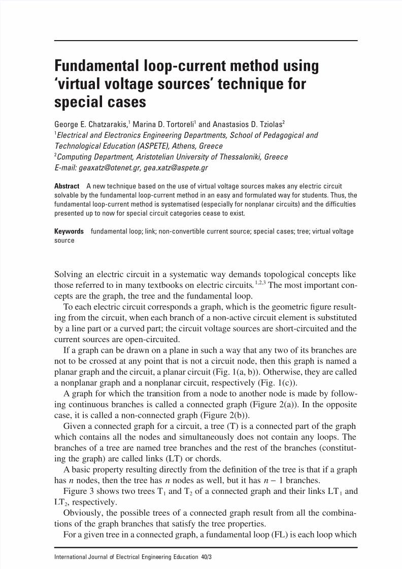
If a graph can be drawn on a plane in such a way that any two of its branches are
not to be crossed at any point that is not a circuit node, then this graph is named a
planar graph and the circuit, a planar circuit (Fig. 1(a, b)). Otherwise, they are called
a nonplanar graph and a nonplanar circuit, respectively (Fig. 1(c)).
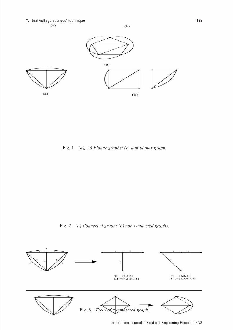
A graph for which the transition from a node to another node is made by follow-ing continuous branches is called a connected graph (Figure 2(a)). In the opposite
case, it is called a non-connected graph (Figure 2(b)).
Given a connected graph for a circuit, a tree (T) is a connected part of the graph
which contains all the nodes and simultaneously does not contain any loops. The
branches of a tree are named tree branches and the rest of the branches (constitut-
ing the graph) are called links (LT) or chords.
A basic property resulting directly from the definition of the tree is that if a graph
has n nodes, then the tree has n nodes as well, but it has n - 1 branches.
Figure 3 shows two trees T1 and T2 of a connected graph and their links LT1 and
LT2, respectively.
Obviously, the possible trees of a connected graph result from all the combina-
tions of the graph branches that satisfy the tree properties.
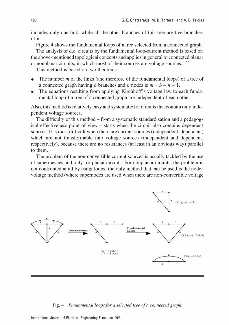
For a given tree in a connected graph, a fundamental loop (FL) is each loop which
5/13/2018 Fundamental Loop Graph Theory 400188 - slidepdf.com
http://slidepdf.com/reader/full/fundamental-loop-graph-theory-400188 2/20
‘Virtual voltage sources’ technique 189
International Journal of Electrical Engineering Education 40/3
Fig. 1 (a), (b) Planar graphs; (c) non-planar graph.
Fig. 2 (a) Connected graph; (b) non-connected graphs.
Fig. 3 Trees of a connected graph.
5/13/2018 Fundamental Loop Graph Theory 400188 - slidepdf.com
http://slidepdf.com/reader/full/fundamental-loop-graph-theory-400188 3/20
includes only one link, while all the other branches of this tree are tree branches
of it.
Figure 4 shows the fundamental loops of a tree selected from a connected graph.
The analysis of d.c. circuits by the fundamental loop-current method is based on
the above-mentioned topological concepts and applies in general to connected planaror nonplanar circuits, in which most of their sources are voltage sources.1,2,5
This method is based on two theorems:
• The number m of the links (and therefore of the fundamental loops) of a tree of
a connected graph having b branches and n nodes is m = b - n + 1.
• The equations resulting from applying Kirchhoff’s voltage law to each funda-
mental loop of a tree of a connected graph are independent of each other.
Also, this method is relatively easy and systematic for circuits that contain only inde-
pendent voltage sources.The difficulty of this method – from a systematic standardisation and a pedagog-
ical effectiveness point of view – starts when the circuit also contains dependent
sources. It is most difficult when there are current sources (independent, dependent)
which are not transformable into voltage sources (independent and dependent,
respectively), because there are no resistances (at least in an obvious way) parallel
to them.
The problem of the non-convertible current sources is usually tackled by the use
of supermeshes and only for planar circuits. For nonplanar circuits, the problem is
not confronted at all by using loops; the only method that can be used is the node-voltage method (where supernodes are used when there are non-convertible voltage
190 G. E. Chatzarakis, M. D. Tortoreli and A. D. Tziolas
International Journal of Electrical Engineering Education 40/3
Fig. 4 Fundamental loops for a selected tree of a connected graph.
5/13/2018 Fundamental Loop Graph Theory 400188 - slidepdf.com
http://slidepdf.com/reader/full/fundamental-loop-graph-theory-400188 4/20
sources).2,4,5 However, the use of supermeshes or supernodes is something that stu-
dents are not able easily to understand and apply; more specifically, the generalisa-
tion and standardisation involved in dealing with special cases in electric circuits is
not easy for them.
This paper, beyond the effort of facing the fundamental loop-current method in asystematic way (especially for nonplanar circuits) also faces the problem of the non-
convertible current sources by introducing the concept of virtual voltage sources.
The term virtual voltage source means that a non-convertible current source (inde-
pendent or dependent) is substituted by a voltage source (independent or dependent
respectively), which has a value equal to the voltage at its terminals and which is
obviously unknown.
Fundamental loop-current methodFacing connected planar and nonplanar circuits in a systematic and standard way
using the fundamental loop-current method depends on the kind of sources that exist
in the circuit and also on whether the existing current sources are convertible or
non-convertible. Based on all these, the fundamental loop-current method can be
examined for four different cases.
Case A. Connected planar or nonplanar circuit with independent (voltage or
current) sources but with all possibly existing current sources convertible
In such a case, the current sources are initially transformed into voltage sources andthen in the resulting equivalent circuit the following steps are executed:
Step 1. From the graph of the circuit, a tree is selected which, as is known, has m
links. Arranging each time a link, a fundamental loop results. Thus, m fundamental
loops are found that correspond to the specific tree which is selected.
Step 2. In all the m fundamental loops, the fundamental loop currents i1, i2, i3,
. . . , im are defined, having any direction.
Step 3. The fundamental loop equations are written in matrix form as follows:
where: Rii, "i = 1, 2, 3, . . . , m denotes the self-resistance of the (FL)i and is equal
to the sum of all resistances of this fundamental loop.
R R R R
R R R R
R R R R
R R R R
i
i
i
i
m
m
m
m m m mm m
11 12 13 1
21 22 23 2
31 32 33 3
1 2 3
1
2
3
. . .
. . .
. . .
. . . . . . .
. . . . . . .
. . . . . . .. . .
.
.
.
È
Î
ÍÍÍÍÍÍÍ
ÍÍ
˘
˚
˙˙˙˙˙˙˙
˙̇
◊
È
Î
ÍÍÍÍÍÍÍ
ÍÍ
˘
˚̊
˙˙˙˙˙˙˙
˙̇
=
È
Î
ÍÍÍÍÍÍÍ
ÍÍ
˘
˚
˙˙˙˙˙˙˙
˙̇
S
S
S
S
v
v
v
vm
1
2
3
.
.
.
‘Virtual voltage sources’ technique 191
International Journal of Electrical Engineering Education 40/3
5/13/2018 Fundamental Loop Graph Theory 400188 - slidepdf.com
http://slidepdf.com/reader/full/fundamental-loop-graph-theory-400188 5/20
Rij = R ji, "i π j, i, j = 1, 2, 3, . . . , m denotes the mutual resistance of the (FL)i
and (FL) j and is equal to the sum of all resistances in the common branches of these
fundamental loops. Its sign is (+) if the loop current directions on the common
branches are the same, otherwise is (-).
Svi, "i = 1, 2, 3, . . . , m is the algebraic sum of the values of all voltage sourcesof the (FL)i. The values of those sources whose loop current goes from the
negative to the positive pole are taken to be positive; otherwise, they are taken to
be negative.
Step 4. The resulting m ¥ m linear system is solved using the Cramer method
or by the matrix inversion method and the currents i1, i2, i3, . . . , im are thus
known.
Step 5. The currents of all branches are calculated combining the fundamental loopcurrents and as a consequence the voltages of all circuit elements are known.
In other words, the solution of the electric circuit is completed.
Notes
• The resistance matrix is symmetrical since Rij = R ji, "i π j.
• There is no particular reason to take the fundamental loop currents in the same
direction, since the sign of the Rij, "i π j is not known from the beginning as in
the mesh current method, but attention must be paid to it.
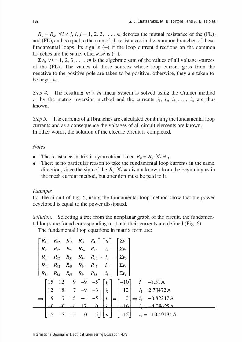
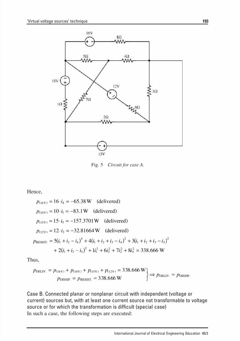
Example
For the circuit of Fig. 5, using the fundamental loop method show that the power
developed is equal to the power dissipated.
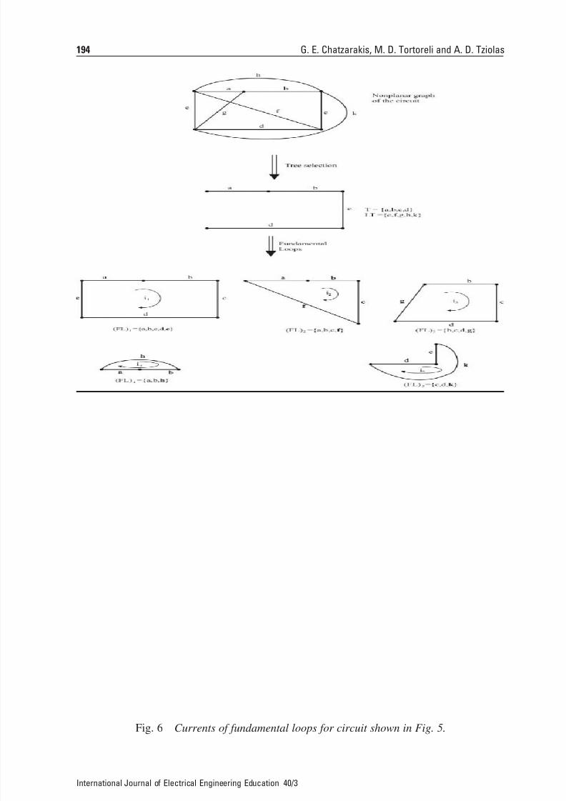
Solution. Selecting a tree from the nonplanar graph of the circuit, the fundamen-
tal loops are found corresponding to it and their currents are defined (Fig. 6).
The fundamental loop equations in matrix form are:
R R R R R
R R R R R
R R R R R
R R R R R
R R R R R
i
i
i
i
i
v
v
v
v
v
11 12 13 14 15
21 22 23 24 25
31 32 33 34 35
41 42 43 44 45
51 52 53 54 55
1
2
3
4
5
1
2
3
4
5
È
Î
ÍÍÍÍÍÍ
˘
˚
˙˙˙˙˙˙
◊
È
Î
ÍÍÍÍÍÍ
˘
˚
˙˙˙˙˙˙
=
È
Î
ÍÍÍÍÍ
SS
S
S
SÍÍ
˘
˚
˙˙˙˙˙˙
fi
- -
- -
- -- - -
- - -
È
Î
ÍÍ
ÍÍÍÍ
˘
˚
˙˙
˙̇˙˙
◊
È
Î
ÍÍ
ÍÍÍÍ
˘
˚
˙˙
˙̇˙˙
=
-
-
-
È
Î
ÍÍ
ÍÍÍÍ
˘
˚
˙˙
˙̇˙˙
fi
15 12 9 9 5
12 18 7 9 3
9 7 16 4 59 9 4 17 0
5 3 5 0 5
10
12
016
15
1
2
3
4
5
i
i
ii
i
ii
i
ii
i
1
2
3
4
5
8 31
2 73472
0 822174 08625
10 49134
= -
=
= -= -
= -
.
.
.
.
.
A
A
AA
A
192 G. E. Chatzarakis, M. D. Tortoreli and A. D. Tziolas
International Journal of Electrical Engineering Education 40/3
5/13/2018 Fundamental Loop Graph Theory 400188 - slidepdf.com
http://slidepdf.com/reader/full/fundamental-loop-graph-theory-400188 6/20
Hence,
Thus,
Case B. Connected planar or nonplanar circuit with independent (voltage or
current) sources but, with at least one current source not transformable to voltage
source or for which the transformation is difficult (special case)
In such a case, the following steps are executed:
p p p p p
p p p p
DELIV. V V V V
DISSIP. RESIST.
DELIV. DISSIP.
W
W
= + + + =
= =¸˝˛
fi =( ) ( ) ( ) ( )16 10 15 12 338 666
338 666
.
.
p i i i i i i i i i i i
i i i i i i i
RESIST.
W
= + -( ) + + + -( ) + + + -( )
+ + -( ) + + + + =
5 4 3
2 1 6 7 8 338 666
1 2 44
1 2 3 42
1 2 3 52
1 3 5
212
22
22
42 .
p i12 212 32 81664V W delivered( ) = ◊ = - ( ).
p i15 515 157 3701V W delivered( ) = ◊ = - ( ).
p i10 110 83 1V W delivered( ) = ◊ = - ( ).
p i16 416 65 38V W delivered( ) = ◊ = - ( ).
‘Virtual voltage sources’ technique 193
International Journal of Electrical Engineering Education 40/3
Fig. 5 Circuit for case A.
5/13/2018 Fundamental Loop Graph Theory 400188 - slidepdf.com
http://slidepdf.com/reader/full/fundamental-loop-graph-theory-400188 7/20
194 G. E. Chatzarakis, M. D. Tortoreli and A. D. Tziolas
International Journal of Electrical Engineering Education 40/3
Fig. 6 Currents of fundamental loops for circuit shown in Fig. 5.
5/13/2018 Fundamental Loop Graph Theory 400188 - slidepdf.com
http://slidepdf.com/reader/full/fundamental-loop-graph-theory-400188 8/20
Step 1. In the locations of the current sources that are non-convertible, virtual
voltage sources are considered with values equal to the corresponding voltage values
present at the terminals of the non-convertible current sources of the given circuit.
Step 2. From the virtual graph of the circuit, a tree is selected which has, as it iswell known m links. Placing each time one link, a fundamental loop results. Thus,
m fundamental loops are found corresponding to the specific selected tree.
Step 3. In all the m fundamental loops, the fundamental loop currents i1, i2, i3,
. . . , im are defined having any direction.
Step 4. The fundamental loop equations are written in matrix form as in case A.
However, in this case the virtual voltage sources are similarly taken as the existing
(non-virtual) ones and they are included in the terms Svi.
Step 5. For each virtual voltage source, an equation is introduced in the matrix that
describes the corresponding non-convertible current source with a linear combina-
tion of the unknown fundamental loop currents of the problem, eliminating each
time an equation that contains a virtual voltage. The remaining equations needed for
the solution are taken from the initial form of the matrix, as they are (those that do
not contain other unknown currents than the fundamental loop currents) or as they
result after the appropriate additions or subtractions in order to eliminate the virtual
voltages appearing initially.By doing so, the new matrix form of the equations does not any longer represent
Ohm’s Law, but it is simply an algebraically m ¥ m equivalent system, which can
lead to the finding of the fundamental loop currents.
Step 6. The resulting m ¥ m linear system is solved as in the previous case and so
the fundamental loop currents are readily available.
Step 7. The currents of all branches are calculated by combining the fundamental
loop currents, and as a consequence, the voltages of all circuit elements are known,
except those at the terminals of the non-convertible current sources (that is the virtual
voltages). The calculation of these voltages is done using the equations eliminated
from the initial form of the system, since the fundamental loop currents are already
known.
In other words, the solution of the electric circuit is completed.
Example
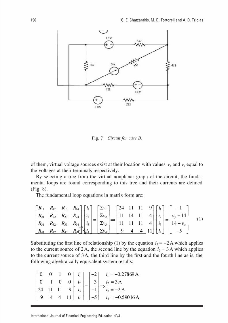
For the circuit of Fig. 7, using the fundamental loop-current method show that the
power developed is equal to the power dissipated.
Solution. Since the independent current sources of the 2A and 3A are non-
convertible (there are no resistances parallel to them), it is considered that, instead
‘Virtual voltage sources’ technique 195
International Journal of Electrical Engineering Education 40/3
5/13/2018 Fundamental Loop Graph Theory 400188 - slidepdf.com
http://slidepdf.com/reader/full/fundamental-loop-graph-theory-400188 9/20
of them, virtual voltage sources exist at their location with values v x and v y equal to
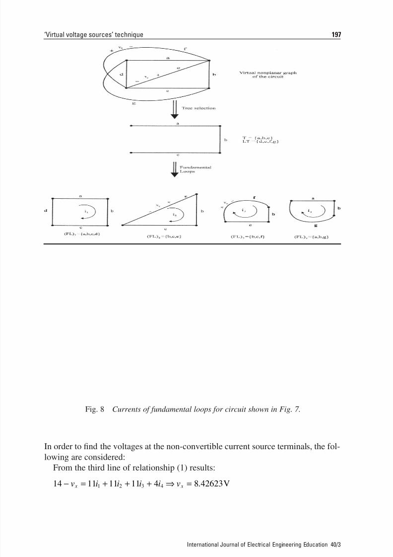
the voltages at their terminals respectively.By selecting a tree from the virtual nonplanar graph of the circuit, the funda-
mental loops are found corresponding to this tree and their currents are defined
(Fig. 8).
The fundamental loop equations in matrix form are:
(1)
Substituting the first line of relationship (1) by the equation i3 = -2A which applies
to the current source of 2A, the second line by the equation i2 = 3A which applies
to the current source of 3A, the third line by the first and the fourth line as is, the
following algebraically equivalent system results:
0 0 1 0
0 1 0 024 11 11 9
9 4 4 11
2
31
5
0 27869
32
0 59016
1
2
3
4
1
2
3
4
È
Î
ÍÍÍÍ
˘
˚
˙̇˙˙
◊
È
Î
ÍÍÍÍ
˘
˚
˙̇˙˙
=
-
-
-
È
Î
ÍÍÍÍ
˘
˚
˙̇˙˙
fi
= -
== -
= -
i
ii
i
i
ii
i
.
.
A
AA
A
R R R R
R R R R
R R R R R R R R
i
i
ii
v
v
vv
11 12 13 14
21 22 23 24
31 32 33 34
41 42 43 44
1
2
3
4
1
2
3
4
24 11 11 9
11 14 11 4
11 11 11 49 4 4 11
È
Î
ÍÍ
ÍÍ
˘
˚
˙˙
˙̇
◊
È
Î
ÍÍ
ÍÍ
˘
˚
˙˙
˙̇
=
È
Î
ÍÍ
ÍÍ
˘
˚
˙˙
˙̇
fi
È
Î
ÍÍ
ÍÍ
˘
˚
˙S
S
SS
˙̇
˙̇
◊
È
Î
ÍÍ
ÍÍ
˘
˚
˙˙
˙̇
=
-
+
--
È
Î
ÍÍ
ÍÍ
˘
˚
˙˙
˙̇
i
i
ii
v
v
y
x
1
2
3
4
1
14
145
196 G. E. Chatzarakis, M. D. Tortoreli and A. D. Tziolas
International Journal of Electrical Engineering Education 40/3
Fig. 7 Circuit for case B.
5/13/2018 Fundamental Loop Graph Theory 400188 - slidepdf.com
http://slidepdf.com/reader/full/fundamental-loop-graph-theory-400188 10/20
‘Virtual voltage sources’ technique 197
International Journal of Electrical Engineering Education 40/3
Fig. 8 Currents of fundamental loops for circuit shown in Fig. 7.
In order to find the voltages at the non-convertible current source terminals, the fol-
lowing are considered:
From the third line of relationship (1) results:
14 11 11 11 4 8 426231 2 3 4- = + + + fi =v i i i i v x x . V
5/13/2018 Fundamental Loop Graph Theory 400188 - slidepdf.com
http://slidepdf.com/reader/full/fundamental-loop-graph-theory-400188 11/20
From the second line of relationship (1) results:
Hence,
Thus,
Case C. Connected planar or nonplanar circuit with independent and dependent
(voltage or current) sources, but with all current sources (independent and
dependent) that possibly exist in the circuit convertible
In this case, the current sources (independent and dependent) are initially trans-formed into voltage sources (independent and dependent respectively), and then in
the resulting equivalent circuit the following steps are executed:
Step 1. From the graph of the circuit, a tree is selected which has, as is well known,
m links. Placing each time one link, a fundamental loop results. Thus, m fundamental
loops are found corresponding to the selected tree.
Step 2. In all the m fundamental loops, the fundamental loop currents i1, i2, i3,
. . . ,im are defined having any direction.
Step 3. The fundamental loop equations are written in matrix form as in case A.
Step 4. The dependent quantities appearing in the matrix form are expressed with
respect to the unknown fundamental loop currents. However, this implies that the
unknown fundamental loop currents appear in the second part of the matrix form of
the equations as well.
Step 5. The elements of the equation lines are rearranged (when needed) so that
the unknown fundamental loop currents appear only in the left-hand part of theequations.
Step 6. The resulting m ¥ m linear system is solved as in the previous cases and
so the fundamental loop currents are readily available.
p p p p p
p p p p p
DELIV. A A V V
DISSIP. RESIST. V
DELIV. DISSIP.
W
W
= + + + =
= + =¸˝˛
fi =( ) ( ) ( ) ( )
( )
3 2 15 14
10
41 70486
41 70486
.
.
p i i i i i i i i i i i iRESIST
W
= +( ) + + + +( ) + + +( ) + + +
=
5 4 7 8 3 2
35 80324
1 42
1 2 3 42
1 2 32
12
22
42
.
p i i i14 1 2 314 10 09834V W delivered( ) = - ◊ + +( ) = - ( ).
p i10 410 5 9016V W dissipated( ) = - ◊ = ( ).
p i i15 1 415 13 03275V W delivered( ) = ◊ +( ) = - ( ).
p v x2 2 16 85246A W delivered( ) = - ◊ = - ( ).
p v y3 3 1 72131A W delivered( ) = - ◊ = - ( ).
v i i i i v y y+ = + + + fi =14 11 14 11 4 0 573771 2 3 4 . V
198 G. E. Chatzarakis, M. D. Tortoreli and A. D. Tziolas
International Journal of Electrical Engineering Education 40/3
5/13/2018 Fundamental Loop Graph Theory 400188 - slidepdf.com
http://slidepdf.com/reader/full/fundamental-loop-graph-theory-400188 12/20
Step 7. The currents of all branches are calculated by combining the funda-
mental loop currents and as a consequence the voltages of all circuit elements are
known.
In other words, the solution of the electric circuit is completed.
Notes
• A dependent current source is considered convertible when there is a resistance
parallel to it and simultaneously the dependent quantity of this or other depen-
dent source is not located at this parallel resistance. If something like this were
to happen, the source transformation would result in the elimination of the
dependent quantity and therefore further steps for the problem solution would
be difficult or even impossible.
•An independent current source is considered convertible when there is a resis-
tance parallel to it and simultaneously the dependent quantity of a dependent
current or voltage source does not appear at this resistance or at the source (for
the same reason as previously referred).
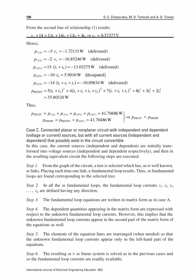
Example
For the circuit of Fig. 9, using the fundamental loop-current method show that the
power developed is equal to the power dissipated.
‘Virtual voltage sources’ technique 199
International Journal of Electrical Engineering Education 40/3
Fig. 9 Circuit for case C.
5/13/2018 Fundamental Loop Graph Theory 400188 - slidepdf.com
http://slidepdf.com/reader/full/fundamental-loop-graph-theory-400188 13/20
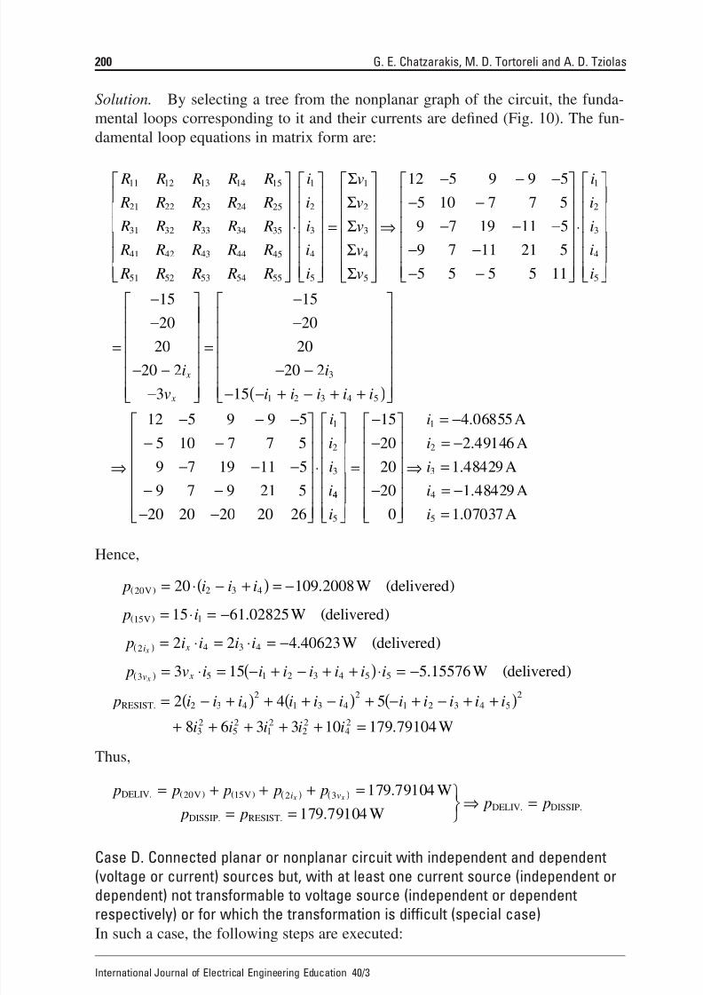
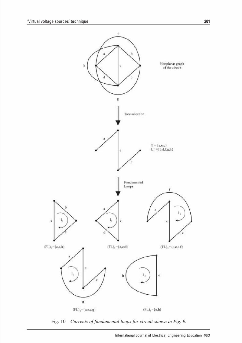
Solution. By selecting a tree from the nonplanar graph of the circuit, the funda-
mental loops corresponding to it and their currents are defined (Fig. 10). The fun-
damental loop equations in matrix form are:
Hence,
Thus,
Case D. Connected planar or nonplanar circuit with independent and dependent
(voltage or current) sources but, with at least one current source (independent or
dependent) not transformable to voltage source (independent or dependent
respectively) or for which the transformation is difficult (special case)
In such a case, the following steps are executed:
p p p p p
p p p p
i v x xDELIV. V V
DISSIP. RESIST.
DELIV. DISSIP.
W
W
= + + + =
= =¸˝˛
fi =( ) ( ) ( ) ( )20 15 2 3 179 79104
179 79104
.
.
p i i i i i i i i i i i
i i i i i
RESIST.
W
= - +( ) + + -( ) + - + - + +( )
+ + + + + =
2 4 5
8 6 3 3 10 179 79104
2 3 42
1 3 42
1 2 3 4 52
32
52
12
22
42 .
p v i i i i i i iv x x3 5 1 2 3 4 5 53 15 5 15576( ) = ◊ = - + - + +( )◊ = - ( ). W delivered
p i i i ii x x2 4 3 42 2 4 40623( ) = ◊ = ◊ = - ( ). W delivered
p i15 115 61 02825V W delivered( ) = ◊ = - ( ).
p i i i20 2 3 420 109 2008V W delivered( ) = ◊ - +( ) = - ( ).
R R R R R
R R R R R
R R R R R
R R R R R
R R R R R
i
i
i
i
i
v
v
v
v
v
11 12 13 14 15
21 22 23 24 25
31 32 33 34 35
41 42 43 44 45
51 52 53 54 55
1
2
3
4
5
1
2
3
4
5
È
Î
ÍÍÍÍÍÍ
˘
˚
˙˙˙˙˙˙
◊
È
Î
ÍÍÍÍÍÍ
˘
˚
˙˙˙˙˙˙
=
È
Î
ÍÍÍÍÍ
SS
S
S
SÍÍ
˘
˚
˙˙˙˙˙˙
fi
- - -- -
- - -
- -
- -
È
Î
ÍÍÍÍÍÍ
˘
˚
˙˙˙˙˙˙
◊
È
Î
ÍÍÍÍÍÍ
˘
˚
˙˙˙˙˙˙
=
-
-
- -
-
È
Î
ÍÍ
ÍÍÍÍ
˘
˚
12 5 9 9 5
5 10 7 7 5
9 7 19 11 5
9 7 11 21 5
5 5 5 5 11
15
20
2020 2
3
1
2
3
4
5
i
i
i
i
i
i
v
x
x
˙̇˙
˙̇˙˙
=
-
-
- -
- - + - + +( )
È
Î
ÍÍ
ÍÍÍÍ
˘
˚
˙˙
˙̇˙˙
fi
- - -
- -
- - -
- -
- -
È
Î
ÍÍÍÍÍÍ
˘
˚
˙˙˙˙˙˙
◊
15
20
2020 2
15
12 5 9 9 5
5 10 7 7 5
9 7 19 11 5
9 7 9 21 5
20 20 20 20 26
3
1 2 3 4 5
1
2
3
i
i i i i i
i
i
i
i44
5
1
2
3
4
5
15
20
20
20
0
4 06855
2 49146
1 48429
1 48429
1 07037i
i
i
i
i
i
È
Î
ÍÍÍÍÍÍ
˘
˚
˙˙˙˙˙˙
=
-
-
-
È
Î
ÍÍÍÍÍÍ
˘
˚
˙˙˙˙˙˙
fi
= -
= -
=
= -
=
.
.
.
.
.
A
A
A
A
A
200 G. E. Chatzarakis, M. D. Tortoreli and A. D. Tziolas
International Journal of Electrical Engineering Education 40/3
5/13/2018 Fundamental Loop Graph Theory 400188 - slidepdf.com
http://slidepdf.com/reader/full/fundamental-loop-graph-theory-400188 14/20
‘Virtual voltage sources’ technique 201
International Journal of Electrical Engineering Education 40/3
Fig. 10 Currents of fundamental loops for circuit shown in Fig. 9.
5/13/2018 Fundamental Loop Graph Theory 400188 - slidepdf.com
http://slidepdf.com/reader/full/fundamental-loop-graph-theory-400188 15/20
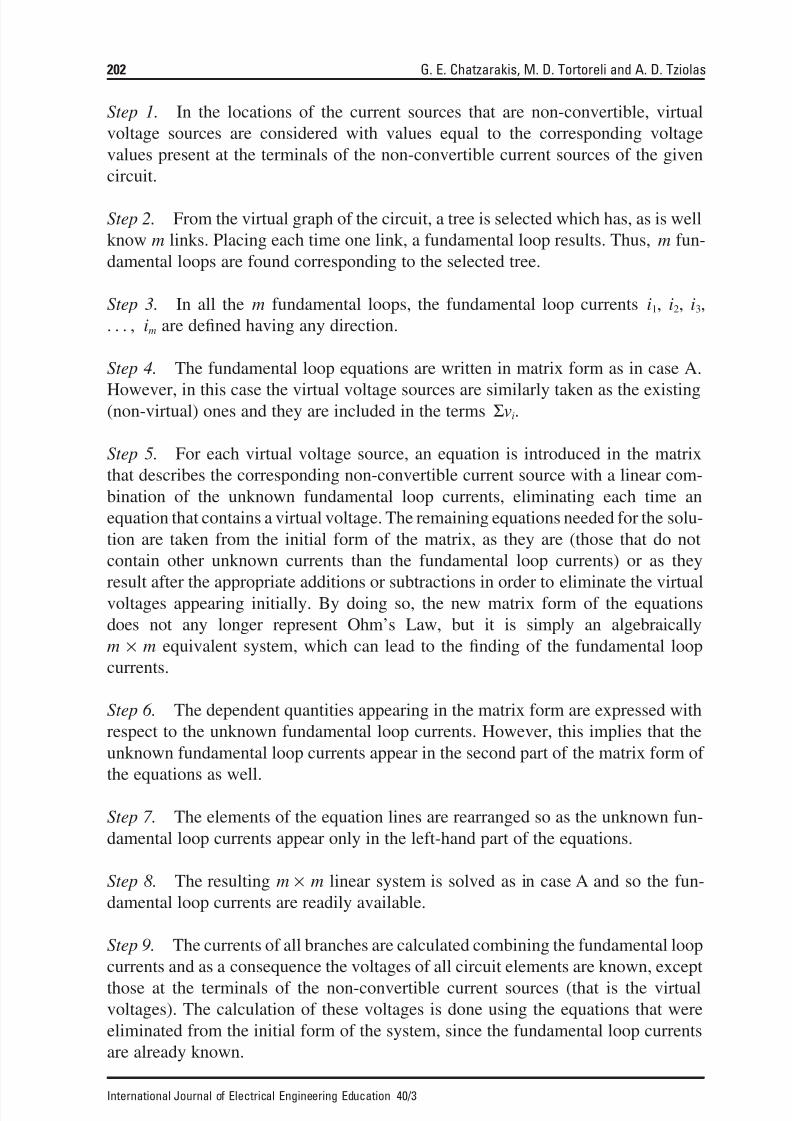
Step 1. In the locations of the current sources that are non-convertible, virtual
voltage sources are considered with values equal to the corresponding voltage
values present at the terminals of the non-convertible current sources of the given
circuit.
Step 2. From the virtual graph of the circuit, a tree is selected which has, as is well
know m links. Placing each time one link, a fundamental loop results. Thus, m fun-
damental loops are found corresponding to the selected tree.
Step 3. In all the m fundamental loops, the fundamental loop currents i1, i2, i3,
. . . , im are defined having any direction.
Step 4. The fundamental loop equations are written in matrix form as in case A.
However, in this case the virtual voltage sources are similarly taken as the existing(non-virtual) ones and they are included in the terms Svi.
Step 5. For each virtual voltage source, an equation is introduced in the matrix
that describes the corresponding non-convertible current source with a linear com-
bination of the unknown fundamental loop currents, eliminating each time an
equation that contains a virtual voltage. The remaining equations needed for the solu-
tion are taken from the initial form of the matrix, as they are (those that do not
contain other unknown currents than the fundamental loop currents) or as they
result after the appropriate additions or subtractions in order to eliminate the virtualvoltages appearing initially. By doing so, the new matrix form of the equations
does not any longer represent Ohm’s Law, but it is simply an algebraically
m ¥ m equivalent system, which can lead to the finding of the fundamental loop
currents.
Step 6. The dependent quantities appearing in the matrix form are expressed with
respect to the unknown fundamental loop currents. However, this implies that the
unknown fundamental loop currents appear in the second part of the matrix form of
the equations as well.
Step 7. The elements of the equation lines are rearranged so as the unknown fun-
damental loop currents appear only in the left-hand part of the equations.
Step 8. The resulting m ¥ m linear system is solved as in case A and so the fun-
damental loop currents are readily available.
Step 9. The currents of all branches are calculated combining the fundamental loop
currents and as a consequence the voltages of all circuit elements are known, except
those at the terminals of the non-convertible current sources (that is the virtual
voltages). The calculation of these voltages is done using the equations that were
eliminated from the initial form of the system, since the fundamental loop currents
are already known.
202 G. E. Chatzarakis, M. D. Tortoreli and A. D. Tziolas
International Journal of Electrical Engineering Education 40/3
5/13/2018 Fundamental Loop Graph Theory 400188 - slidepdf.com
http://slidepdf.com/reader/full/fundamental-loop-graph-theory-400188 16/20
In other words, the solution of the electric circuit is completed.
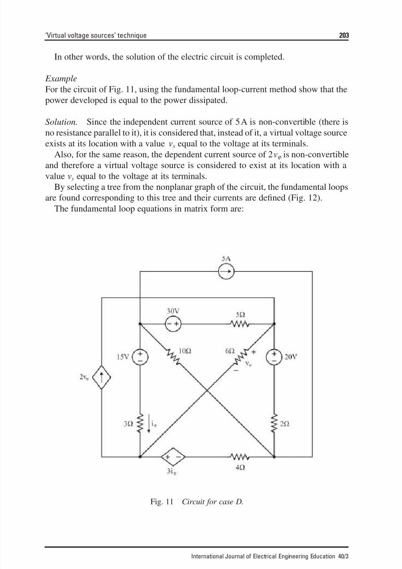
Example
For the circuit of Fig. 11, using the fundamental loop-current method show that the
power developed is equal to the power dissipated.
Solution. Since the independent current source of 5A is non-convertible (there is
no resistance parallel to it), it is considered that, instead of it, a virtual voltage source
exists at its location with a value v x equal to the voltage at its terminals.
Also, for the same reason, the dependent current source of 2vj is non-convertible
and therefore a virtual voltage source is considered to exist at its location with a
value v y equal to the voltage at its terminals.
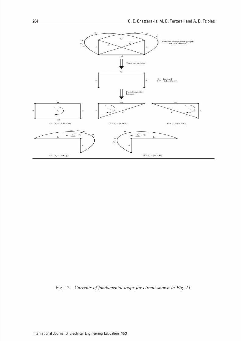
By selecting a tree from the nonplanar graph of the circuit, the fundamental loops
are found corresponding to this tree and their currents are defined (Fig. 12).The fundamental loop equations in matrix form are:
‘Virtual voltage sources’ technique 203
International Journal of Electrical Engineering Education 40/3
Fig. 11 Circuit for case D.
5/13/2018 Fundamental Loop Graph Theory 400188 - slidepdf.com
http://slidepdf.com/reader/full/fundamental-loop-graph-theory-400188 17/20
204 G. E. Chatzarakis, M. D. Tortoreli and A. D. Tziolas
International Journal of Electrical Engineering Education 40/3
Fig. 12 Currents of fundamental loops for circuit shown in Fig. 11.
5/13/2018 Fundamental Loop Graph Theory 400188 - slidepdf.com
http://slidepdf.com/reader/full/fundamental-loop-graph-theory-400188 18/20
Substituting the first line of relationship (2) by the equation i4 = 5A which appliesto the independent current source of 5A, the second line by the equation i5 = 2vj
which applies to the dependent current source of 2vj , the third line by the first, the
fourth line by the second and the fifth line by the third, the following algebraically
equivalent system results:
In order to find the voltages at the non-convertible current source terminals the fol-lowing are considered:
The fourth line of relationship (2) gives:
The fifth line of relationship (2) gives:
Hence,
p i i i i i30 1 2 3 4 530 158 2365V W delivered( ) = - ◊ + + - -( ) = - ( ).
p v v i vv y y2 22 12 186 39171
j j( ) = - ◊ = - ◊ = - ( ). W delivered
p v x5 5 42 37745A W delivered( ) = - ◊ = - ( ).
- + = - - - + + fi = -45 8 8 5 5 8 9 653781 2 3 4 5v i i i i i v y y . V
- + = - - - + + fi =10 7 5 7 7 5 8 475491 2 3 4 5v i i i i i v x x . V
0 0 0 1 0
0 0 0 0 1
14 8 7 7 8
8 14 5 5 8
7 5 17 7 5
5
2
25 3
45
10
5
12
25 3
1
2
3
4
5
2
1 2- -
- -- -
È
Î
ÍÍÍ
ÍÍÍ
˘
˚
˙˙˙
˙̇˙
◊
È
Î
ÍÍÍ
ÍÍÍ
˘
˚
˙˙˙
˙̇˙
= +
È
Î
ÍÍÍ
ÍÍÍ
˘
˚
˙˙˙
˙̇˙
= + - - +
i
i
i
i
i
v
i
i
i i
j
j ii
i
i
i
i
i
5
1
2
3
4
5
45
10
0 0 0 1 0
0 12 0 0 1
17 11 7 7 11
8 14 5 5 8
7 5 17 7 5
5
0
25
45
10
( )
È
Î
ÍÍÍ
ÍÍÍ
˘
˚
˙˙˙
˙̇˙
fi
-
- -
- -
- -
È
Î
ÍÍÍÍÍÍ
˘
˚
˙˙˙˙˙˙
◊
È
Î
ÍÍÍÍÍÍ
˘
˚
˙˙˙˙˙˙
=
È
Î
ÍÍÍÍÍÍ
˘
˚
˙˙˙̇˙˙˙
fi
= -
= -
=
=
= -
i
i
i
i
i
1
2
3
4
5
8 27166
1 60897
0 84754
5
19 30764
.
.
.
.
A
A
A
A
A
( )2
R R R R R
R R R R R
R R R R R
R R R R R
R R R R R
i
i
i
i
i
v
v
v
v
v
11 12 13 14 15
21 22 23 24 25
31 32 33 34 35
41 42 43 44 45
51 52 53 54 55
1
2
3
4
5
1
2
3
4
5
È
Î
ÍÍÍ
ÍÍÍ
˘
˚
˙˙˙
˙̇˙
◊
È
Î
ÍÍÍ
ÍÍÍ
˘
˚
˙˙˙
˙̇˙
=
È
Î
ÍÍÍ
ÍÍ
S
S
S
SSÍÍ
˘
˚
˙˙˙
˙̇˙
fi
- -
- -
- -
- - -
- - -
È
Î
ÍÍÍÍÍÍ
˘
˚
˙˙˙˙˙˙
◊
È
Î
ÍÍÍÍÍÍ
˘
˚
˙˙˙˙˙˙
=
+
- +
- +
È
Î
ÍÍÍÍÍÍ
14 8 7 7 8
8 14 5 5 8
7 5 17 7 5
7 5 7 7 5
8 8 5 5 8
25 3
45
10
10
45
1
2
3
4
5
i
i
i
i
i
i
v
v
x
y
j ˘̆
˚
˙˙˙˙˙˙
‘Virtual voltage sources’ technique 205
International Journal of Electrical Engineering Education 40/3
5/13/2018 Fundamental Loop Graph Theory 400188 - slidepdf.com
http://slidepdf.com/reader/full/fundamental-loop-graph-theory-400188 19/20
Thus,
Conclusions
The classification of connected planar or nonplanar electric circuits into four cate-
gories, as have been examined in this paper, enables the student to solve easily, fol-
lowing similar procedures, any circuit by the fundamental loop-current method.
However, this method basically applies to nonplanar circuits for which the mesh-
current method cannot be used. For planar circuits, the mesh-current method can be
applied and its use is recommended, since it is an easier method than the funda-
mental loop-current method. Therefore, all the examples presented in this article dealwith nonplanar circuits.
With respect to the special cases, the second and fourth (B, D) dealt with virtual
voltage sources; this results in the non-differentiation of these cases regarding the
overall methodological steps to be followed.
Another equally important advantage of using virtual voltage sources is the imme-
diate finding of the voltages present at the terminals of the non-convertible current
sources, given that the fundamental loop currents are known, since their voltages
are already expressed by the way the equations are written in matrix form. So, the
power developed by these sources is easy to calculate and therefore the proof of thepower balance does not present any difficulties.
Special attention must be paid to the conditions under which a current source is
transformed to a voltage source; this is because whereas a current source is con-
vertible when there is a resistance parallel to it, for methodological purposes it
should be considered non-convertible, when the conditions mentioned in the fourth
case (D) are not met.
Finally, the fundamental loop-current method, as has been analysed already, can
obviously be used for circuits in the sinusoidal steady state (a.c. circuits). However,
the necessary condition is that all circuit sources are of the same frequency (other-
wise the principle of superposition is used). So, if all sources are of the same fre-
quency, the fundamental loop-current method starts after the circuit transformation
to the frequency domain.
p p p p p p p
p p
p p
v V iDELIV. A V V
DISSIP. RESIST.
DELIV. DISSIP.
W
W
= + + + + + =
= =¸˝˛
fi =
( ) ( ) ( ) ( ) ( ) ( )5 2 30 20 15 31010 82484
1010 82484j j
.
.
p i i i i i i i i i i i i
i i
RESIST.
W
= + + - -( ) + + -( ) + + - - +( )
+ + =
5 2 4 3
10 6 1010 82484
1 2 3 4 5
21 3 4
212
1 2 5
2
32
22 .
p i i i i i ii3 1 1 2 5 13 3 233 93106j j( ) = - ◊ = - - - +( )◊ = - ( ). W delivered
p i i i i15 1 2 515 15 141 40515V W delivered( ) = ◊ = ◊ - - +( ) = - ( )j .
p i i i20 1 3 420 248 4824V W delivered( ) = ◊ + -( ) = - ( ).
206 G. E. Chatzarakis, M. D. Tortoreli and A. D. Tziolas
International Journal of Electrical Engineering Education 40/3
5/13/2018 Fundamental Loop Graph Theory 400188 - slidepdf.com
http://slidepdf.com/reader/full/fundamental-loop-graph-theory-400188 20/20
References
1 G. E. Chatzarakis, Electric Circuits, vol. II (Tziolas, Thessaloniki, 2000).
2 J. W. Nilsson and A. Susan Riedel, Electric Circuits (Addison Wesley, New York, 1996).
3 C. A. Desoer and S. Ernest Kuh, Basic Circuit Theory (McGraw–Hill, New York, 1969).
4 C. K. Alexander and N. O. Matthew Sadiku, Fundamentals of Electric Circuits (McGraw–Hill, NewYork, 2000).
5 W. H. Hayt and E. Jack Kemmerly, Engineering Circuit Analysis (McGraw–Hill, New York, 1993).
‘Virtual voltage sources’ technique 207
International Journal of Electrical Engineering Education 40/3


![Classi cation of graph metrics - Delft University of ... · protocols (e.g. BGP) have built-in loop prevention algorithms. 2.1.6 Expansion The expansion e h of a graph [1] is the](https://img.pdfslide.net/doc/110x75/5ed077b0a74b8d03714a0937/classi-cation-of-graph-metrics-delft-university-of-protocols-eg-bgp-have.jpg)