Embed Size (px)
Citation preview
Otto-von-Guericke University MagdeburgFaculty of Computer Science
Department for Simulation and Graphics
Diploma Thesis
Fundamental Permutation Group Algorithms forSymmetry Computation
Author:
Thomas RehnJanuary 12, 2010
Supervisors:
Prof. Dr. rer. nat. habil. Stefan SchirraOtto-von-Guericke University Magdeburg
Faculty of Computer SciencePostfach 4120, D–39016 Magdeburg
Germany
Priv.-Doz. Dr. rer. nat. habil. Achill SchürmannInstitute of Applied MathematicsDelft University of Technology
Mekelweg 42628 CD DelftThe Netherlands

Rehn, Thomas:Fundamental Permutation Group Algorithms for Sym-metry ComputationDiploma Thesis, Otto-von-Guericke University Magdeburg,January 2010.
This document is licensed under a Creative CommonsAttribution-Share Alike 3.0 License:http://creativecommons.org/licenses/by-sa/3.0

Contents
List of Figures iii
List of Algorithms iv
1 Introduction 1
1.1 Motivation . . . . . . . . . . . . . . . . . . . . . . . . . . . . . . . . . . . 1
1.2 Permutations and notation . . . . . . . . . . . . . . . . . . . . . . . . . . 2
2 Introduction to Bases and Strong Generating Sets 5
2.1 DeVnitions . . . . . . . . . . . . . . . . . . . . . . . . . . . . . . . . . . . 5
2.2 Elementary algorithms & data structures . . . . . . . . . . . . . . . . . . . 7
2.2.1 Orbits and transversals . . . . . . . . . . . . . . . . . . . . . . . . 7
2.2.2 Sifting . . . . . . . . . . . . . . . . . . . . . . . . . . . . . . . . . 10
2.3 BSGS construction with Schreier-Sims algorithm . . . . . . . . . . . . . . 11
2.4 Transversal revisited – shallow Schreier trees . . . . . . . . . . . . . . . . 14
2.5 Base change . . . . . . . . . . . . . . . . . . . . . . . . . . . . . . . . . . 17
2.5.1 Deterministic base point transposition . . . . . . . . . . . . . . . . 17
2.5.2 Randomized base point transposition . . . . . . . . . . . . . . . . 18
2.5.3 Base change by conjugation . . . . . . . . . . . . . . . . . . . . . 21
2.5.4 Base change by construction – randomized BSGS construction . . 21
3 Backtrack Search 25
3.1 Classical backtracking . . . . . . . . . . . . . . . . . . . . . . . . . . . . . 26
3.1.1 Search tree . . . . . . . . . . . . . . . . . . . . . . . . . . . . . . . 27
3.1.2 Pruning the tree . . . . . . . . . . . . . . . . . . . . . . . . . . . . 28
3.1.3 Double coset minimality . . . . . . . . . . . . . . . . . . . . . . . 30
3.1.4 Problem-dependent pruning . . . . . . . . . . . . . . . . . . . . . 31
3.1.5 Coset representative search . . . . . . . . . . . . . . . . . . . . . . 35
3.2 Partition backtracking . . . . . . . . . . . . . . . . . . . . . . . . . . . . . 36
3.2.1 Introduction to partitions . . . . . . . . . . . . . . . . . . . . . . . 37
i

Contents
3.2.2 Search tree . . . . . . . . . . . . . . . . . . . . . . . . . . . . . . . 39
3.2.3 Constructing an R-base . . . . . . . . . . . . . . . . . . . . . . . . 43
3.2.4 Pruning the tree . . . . . . . . . . . . . . . . . . . . . . . . . . . . 45
3.2.5 Coset representative search . . . . . . . . . . . . . . . . . . . . . . 47
4 Implementation 49
4.1 Low-level data structures . . . . . . . . . . . . . . . . . . . . . . . . . . . 49
4.1.1 Permutation . . . . . . . . . . . . . . . . . . . . . . . . . . . . . . 49
4.1.2 Partition . . . . . . . . . . . . . . . . . . . . . . . . . . . . . . . . 50
4.2 Experiments . . . . . . . . . . . . . . . . . . . . . . . . . . . . . . . . . . 52
4.2.1 Data acquisition and setup . . . . . . . . . . . . . . . . . . . . . . 53
4.2.2 BSGS construction . . . . . . . . . . . . . . . . . . . . . . . . . . 53
4.2.3 Base change . . . . . . . . . . . . . . . . . . . . . . . . . . . . . . 57
4.2.4 Subgroup search: setwise stabilizer . . . . . . . . . . . . . . . . . . 61
4.2.5 Subgroup search: group intersection . . . . . . . . . . . . . . . . . 65
4.2.6 Summary . . . . . . . . . . . . . . . . . . . . . . . . . . . . . . . 67
5 Conclusion 69
5.1 Summary . . . . . . . . . . . . . . . . . . . . . . . . . . . . . . . . . . . . 69
5.2 Outlook . . . . . . . . . . . . . . . . . . . . . . . . . . . . . . . . . . . . . 70
A PermLib 71
Nomenclature 73
References 74
Bibliography . . . . . . . . . . . . . . . . . . . . . . . . . . . . . . . . . . . . . 74
Software . . . . . . . . . . . . . . . . . . . . . . . . . . . . . . . . . . . . . . . . 76
Index 77
ii

List of Figures
2.1 A Schreier tree for the orbit of 1 under action of G = 〈a, b〉 as in Example2.6 . . . . . . . . . . . . . . . . . . . . . . . . . . . . . . . . . . . . . . . . 8
2.2 Schreier vector encoding for Figure 2.1 with l0 = (), l1 = a−, l2 = b− . . . 92.3 Explicit transversal as vector for Figure 2.1 . . . . . . . . . . . . . . . . . . 92.4 Asymptotic time and memory requirements for diUerent transversal im-
plementations . . . . . . . . . . . . . . . . . . . . . . . . . . . . . . . . . 15
3.1 Polyhedral cones . . . . . . . . . . . . . . . . . . . . . . . . . . . . . . . . 253.2 Group with twelve elements split up into cosets by a search tree . . . . . . 273.3 Graph automorphism example . . . . . . . . . . . . . . . . . . . . . . . . 363.4 Overview of P-reVnements for diUerent problems . . . . . . . . . . . . . . 48
4.1 Example intersection of a partition (. . . | 1 2 3 6 7 8 | . . . ) with 2, 6, 7 . . 524.2 Base construction average times for primitive permutation groups . . . . . 544.3 Base construction times for symmetric groups . . . . . . . . . . . . . . . . 564.4 Base construction times for polyhedral automorphism groups . . . . . . . 564.5 Base change/transposition average times for selected primitive groups . . . 584.6 Base change average times for selected primitive groups . . . . . . . . . . 594.7 Base change average times for selected primitive groups and similar sets . 594.8 Base change times for polyhedral automorphism groups . . . . . . . . . . 604.9 Set stabilizer search average times for primitive groups . . . . . . . . . . . 614.10 Set stabilizer search time depending on set size . . . . . . . . . . . . . . . 624.11 Set stabilizer search average times with enhanced double coset pruning for
primitive groups . . . . . . . . . . . . . . . . . . . . . . . . . . . . . . . . 634.12 Set stabilizer search times for polyhedral automorphism groups . . . . . . 644.13 Set stabilizer search times for symmetric groups . . . . . . . . . . . . . . . 644.14 Intersection search times for primitive groups . . . . . . . . . . . . . . . . 654.15 Number of nodes visited during intersection search for primitive groups . . 664.16 Intersection search times for primitive groups . . . . . . . . . . . . . . . . 66
iii

List of Algorithms
2.1 Orbit . . . . . . . . . . . . . . . . . . . . . . . . . . . . . . . . . . . . . . . 72.2 Orbit and Schreier tree . . . . . . . . . . . . . . . . . . . . . . . . . . . . . 92.3 Sifting . . . . . . . . . . . . . . . . . . . . . . . . . . . . . . . . . . . . . . 102.4 Schreier-Sims BSGS construction . . . . . . . . . . . . . . . . . . . . . . . . 132.5 Orbit and shallow Schreier tree . . . . . . . . . . . . . . . . . . . . . . . . . 162.6 Base change with transpositions . . . . . . . . . . . . . . . . . . . . . . . . 182.7 Base point transposition – deterministic version . . . . . . . . . . . . . . . . 192.8 Base point transposition – randomized version . . . . . . . . . . . . . . . . 202.9 Base change with conjugation and transpositions . . . . . . . . . . . . . . . 222.10 Randomized Schreier-Sims BSGS construction . . . . . . . . . . . . . . . . 233.1 Depth-Vrst traversal of the search tree of a group . . . . . . . . . . . . . . . 283.2 Backtrack subgroup search with elementary pruning . . . . . . . . . . . . . 293.3 Subgroup search with elementary double coset pruning . . . . . . . . . . . 323.4 Set stabilizer search with elementary double coset pruning . . . . . . . . . . 343.5 Set stabilizer search setup . . . . . . . . . . . . . . . . . . . . . . . . . . . . 353.6 Recover group element from given (partial) base image . . . . . . . . . . . . 413.7 Partition backtrack subgroup search with very basic pruning . . . . . . . . . 423.8 R-base construction for a set stabilization problem . . . . . . . . . . . . . . 453.9 Partition backtrack subgroup search with elementary pruning . . . . . . . . 46
iv
1 Introduction
1.1 Motivation
Over the last 40 years powerful algorithmic methods have been developed for many prob-lems in algebra. Along with others, the so called computational group theory that dealswith algorithms for problems of group theory has grown to a mature tool (cf. [CH92]).With more and more practical algorithms getting available and ever-growing computerpower, the usage of group theory has reached into many areas of mathematics and othernatural sciences. The book [Ker99], for instance, provides a very good overview of theapplicability of group theory to combinatorial objects from many applications.
From highly successful single-purpose applications like graph theory (cf. [McK81] andthe software [nauty]) more general methods have evolved for the computation with sym-metries or auto- and isomorphisms. These are applicable to matrices, codes, designs,graphs and groups alike [Leo84, BL85, Leo91, McK98, Bri00]. Other areas have proVtedfrom this progress and are able to handle or exploit symmetries in their problems, whichhelps to extend the realm of practically solvable problems and instances. Just to namea few of these applications, [Jun03] examines symmetry of petri-nets. [KÖ06] describemethods to classify codes and designs isomorphism-free. [Mar09] shows in his surveythe impact of symmetry to integer programming. [BSS09] enumerate vertices and rays ofpolyhedra up to the immanent symmetry of the geometric object. Mathematically, thissymmetry computation part translates into computations with and search in permutationgroups.
All these examples have in common that they use diUerent tools to handle the ba-sic symmetry part of their real computational task. Either they implement permutationgroup algorithms in own code for this fundamental recurring problem or use well-testedgroup theoretic software like the open-source algebra system GAP [GAP] or the commer-cial Magma [Magma]. These software packages, however, lack proper and simple APIs tobe used from C or C++, still the language of choice in many projects, and cause hugedependencies. There also exists an open source C implementation for such permutationgroup problems by Leon from 1991 [Leo91], but it is designed as a pure stand-alone pro-gram and not as callable library. Moreover, it has too many memory leaks and errors tobe used as such. Since 2008 there also have been eUorts of the open source Sage project[Sage] to provide implementations of automorphism and permutation group algorithmsas part of their package (cf. [Mila, Milb]). To date only the former part is complete.
There are many excellent books available that cover group algorithms, for example[But91], [Ser03] and [HEO05], but these rather aim at more sophisticated Velds of compu-tational group theory and do not go into implementation details, which may be of interestfor practitioners from other areas. This is especially true for the allegedly fast partitionbacktrack methods of Leon, which most books cover, if at all, only in a very abstract way,
1

1 Introduction
hiding the diXculties an implementation may face. This thesis presents the very basictechniques to solve the group theoretic part of common problems in symmetry computa-tions along with an implementation of all algorithms as a C++ library, christened PermLib.We begin in Chapter 2 with a look at fundamental data structures and algorithms to
work with permutation groups. Because permutation groups usually consist of a hugenumber of elements they are not given as a complete set of permutations, but only afew generating elements are known, from which all other elements can be derived. Thisalready causes problems with the simple task of group membership testing. We will lookat a data structure called base and strong generating set which allows a representation ofa group such that this and other very basic problems can be solved eXciently.Having learned about suitable structures to store permutation groups, in Chapter 3 we
will deal with searching for speciVc subgroups or elements in a permutation group. There-fore we will analyze two diUerent general purpose backtracking algorithms. As an examplewe will study the special cases of set stabilizers and group intersections.In Chapter 4 we will look at speciVc implementation details and the results of experi-
ments with the PermLib. There we will see the algorithms’ and implementation’s limits,potential and potential pitfalls, some of which have to the best of the author’s knowledgenot been extensively discussed in public. Chapter 5 provides a summary of our Vndings aswell as an outlook into possible future work.
1.2 Permutations and notation
A fundamental object that we will work with all the time are permutations. Permutationsare bijections from a set Ω to itself. This set could be vertices or facets of a polyhedron,vertices of a graph, variables in an equation system and many other things, but we identifyΩ without loss of generality with the set of numbers 1, . . . , n, n := |Ω|. There are twodiUerent ways to specify the bijection of a permutation. The Vrst way is to give the imageof each ω ∈ Ω explicitly, the so called image form. In this thesis we will use the secondway, that is cycle notation: a cycle is a sequence ω1, ω2, . . . , ωk such that• ω2 is the image of ω1,
• ω3 is the image of ω2,
• . . .
• ωk is the image of ωk−1 and
• ω1 is the image of ωk.We can write a permutation as a sequence of disjoint cycles, which is called cycle form.
Example 1.1. Consider Ω = 1, 2, 3, 4, 5, 6 and the permutation g with the followingimage:
1 2 3 4 5 62 3 1 4 6 5
where the Vrst row lists all elements of Ω and the second row their images under g. Weobserve that g has three disjoint cycles (1 2 3), (4) and (5 6). We omit the cycle of length1 and write g = (1 2 3)(5 6), or equivalently g = (5 6)(1 2 3), because for disjoint cyclesorder does not matter.
2
1.2 Permutations and notation
As we use cycle notation for permutations, we write () for the identity permutation.Permutations on the same set with the concatenation operation build a group. Becausethe notation of this concatenation resembles a multiplicative operation we usually saythat permutations are multiplied. The interested reader may Vnd in [But91, Ch. 2] moreexamples of permutations and also a very good introduction to groups, which is not givenhere. In the following we will establish notation for groups that we use throughout thisthesis.If a group G is Vnitely generated by some elements g1, . . . , gk we write G =〈g1, . . . , gk〉. For two groups G,H we denote with G ≤ H that G is a subgroup of H .The number of elements in G is called order of G and we denote it by |G|. Furthermore,we stick to Knuth [Knu91] for his compact notation of group inverses, so g− shall be theinverse element of g.As for this thesis we are especially interested in symmetries within a Vnite set of objects,
we always consider a permutation group G ≤ Sym(Ω) acting on a Vnite set Ω, where Gis a subgroup of the group Sym(Ω) of all permutations of Ω. We call the minimal size |Ω|such that G is properly deVned the degree of G. Of course we can always trivially extendG ≤ Sym(Ω) to a subgroup of some Sym(Ω′) where Ω′ ⊃ Ω. Lowercase Greek letterswill denote elements of Ω and we use lower- and uppercase Latin letters for elements andsubgroups of the group Sym(Ω).We write αg for the action of g ∈ G on α ∈ Ω and this action will be left-associative,
i.e. αgh = (αg)h. The orbit of α under G is the set of images αG := αg : g ∈ G.
Example 1.2. Consider Ω = 1, . . . , 6 and G = 〈a, b〉 generated by a = (1 4 5)(2 3 6),b = (2 3 1 6), denoted in cycle form. Then we have b− = (2 6 1 3), 1a = 4, 1ba = 6a = 2and orbits 1〈b〉 = 1, 2, 3, 6 and 1G = Ω.
Let H,K ≤ G be subgroups of G and g ∈ G. Then we deVne the right coset Hg :=hg : h ∈ H and analogously the left coset gH := gh : h ∈ H. The double cosetHgK is given by HgK := hgk : h ∈ H, k ∈ K. As becomes immediately clear fromthe deVnition, two cosets Hg1, Hg2 are either the same or disjoint. Because every g ∈ Gis in one coset, G is partitioned by its cosets. Thus it makes sense to deVne a right (left)transversal U ⊆ G for G modulo H as a set containing exactly one representative ofevery H-right (left) coset of G, including the identity () ∈ U .For every subgroup H we can deVne the index |G : H| of H in G as the number of
right (or equivalently: left) cosets of H in G. With this notation at hand we can remindourselves of Lagrange’s Theorem.
Theorem 1.3 (Lagrange’s Theorem). LetG be a Vnite group andH a subgroup ofG. Then|G| = |G : H| · |H|.
Proof. As we have already seen G can be partitioned into its cosets moduloH . Let U be atransversal for G modulo H . Then we have
|G| =∑u∈U
|Hu|. (1.1)
Furthermore, for every cosetHa and g ∈ G we have |Ha| = |Hag|. So it holds especiallythat |Ha| = |Ha(a−b)| = |Hb|. It follows that every summand in (1.1) is of the same size,resulting in |G| = |U | · |H()| = |G : H| · |H|.
3
1 Introduction
An immediate consequence of this proof is the following corollary.
Corollary 1.4. Let G and H as above and U a transversal for G modulo H . Every g ∈ Gcan uniquely be written as g = uh where u ∈ U and h ∈ H .
Example 1.5. Let Ω = 1, 2, 3, 4 and G = S4 = 〈(1 2), (2 3), (3 4)〉 the symmetricgroup of four elements. Then H := 〈(1 2), (2 3)〉 ≤ G is a subgroup of G. There are|G : H| = |G|
|H| = 246
= 4 right cosets of H in G: the right cosets H(), H(3 4), H(2 4) andH(1 4), corresponding to the four possible images of the remaining point 4. Thus the fourelements U := (), (3 4), (2 4), (1 4) form a transversal of G modulo H .
The stabilizer Gα of α in G is deVned as the set Gα := g ∈ G : αg = α and formsa subgroup of G. In the same manner we can deVne the pointwise stabilizer of a tuple(α1, . . . , αk) as G(α1,...,αk) := g ∈ G : ∀1 ≤ i ≤ k : αgi = αi and the stabilizer ofa set α1, . . . , αk as Gα1,...,αk := g ∈ G : ∀1 ≤ i ≤ k : ∃j : αgi = αj. Notethe diUerence in notation between pointwise stabilizer G(α1,...,αk) and setwise stabilizerGα1,...,αk.
Example 1.6. Let again Ω = 1, 2, 3, 4 and G = S4 = 〈(1 2), (2 3), (3 4)〉. Then G1 =〈(2 3), (3 4)〉, G(1,2) = 〈(3 4)〉 and G1,2 = 〈(1 2), (3 4)〉.
4

2 Introduction to Bases and StrongGenerating Sets
To work with permutation groups we need a suitable structure to represent them onthe computer. Usually we are given a group G ≤ Sym(Ω) by a list of generatorsS = s1, s2, . . . , sk with G = 〈S〉. If we want to search for group elements with speciVcproperties as in Chapter 3 we are confronted with a problem: We know that each elementis a product of elements of S but we have no eXcient means to systematically enumerateall elements of G, for example for an exhaustive search. The reverse problem also exists:given some x ∈ Sym(Ω), we cannot decide whether x ∈ G. This is a real obstacle forsystematic search approaches.
In 1970 Sims introduced the concept of a base for computations with permutation groupsto overcome these diXculties (cf. [Sim70, Sim71a]). Similarly to a base in vector spacesgroup elements have a unique representation relative to it. Such a base also allows easygroup membership testing, in this context usually called “sifting”.
First we will look at the fundamental concepts of bases. Before we see how to set up abase and the related strong generating sets for a permutation group we have to examinediUerent ways to store orbits and transversals and to solve the group membership problemusing bases. After the base construction with the Schreier-Sims algorithm we will look attwo other tools for the eXcient use of bases: an improved algorithm to compute transver-sals and base change algorithms. Again similarly to vector spaces, one certain base ismore comfortable in some contexts to work with than another, so we will see how we cantransform a base without re-constructing it from scratch.
2.1 DeVnitions
DeVnition 2.1. Let G be a Vnite permutation group acting on the set 1, . . . , n. We calla sequence of elements B := (β1, β2, . . . , βm) a base for G if the only element of G to VxB pointwise is the identity.
For a base B we denote by G[i] := G(β1,...,βi−1) the pointwise stabilizer of the i− 1 Vrstbase elements (β1, . . . , βi−1) which form a subgroup chain, the stabilizer chain:
G = G[1] ≥ G[2] ≥ · · · ≥ G[m] ≥ G[m+1] = 〈()〉. (2.1)
If every G[i+1] is a proper subgroup of G[i] we call the base B nonredundant.
The cosets of G[i] modulo G[i+1] are closely related to the orbits βG[i]
i . For two cosetsG[i+1]a = G[i+1]b with a, b ∈ G[i] we have a = hb for h ∈ G[i+1] and thus βai =βhbi = βbi because h stabilizes βi. Also the reverse direction holds: From βai = βbi we can
5

2 Introduction to Bases and Strong Generating Sets
immediately conclude that the two cosets G[i+1]a, G[i+1]b are the same. So we can builda transversal for G[i] modulo G[i+1], which contains one representative for every coset, bylooking at elements generating the orbit ∆(i) := βG
[i]
i . For every β ∈ ∆(i) let uβ ∈ G[i] bean element that maps βi to β, i. e. β
uβi = β. Then it follows from our considerations that
U (i) := uβ : β ∈ ∆(i) is a (right) transversal for G[i] modulo G[i+1]. We call ∆(i) thei-th fundamental orbit.
Example 2.2. Let Ω = 1, 2, 3, 4 andG = S4 the symmetric group of four elements. Thesequence (4, 3) is not a base because the permutation (1 2) stabilizes the tuple pointwise.If we add 2 to the list we get a base (4, 3, 2) because the image of 3 = 4− 1 points alreadydetermines a permutation: (4, 3, 2)g = (4, 3, 2) implies g = ().The stabilizer chain consists of
G[1] = G = S4
G[2] = G(4) = 〈(1 2), (2 3)〉 ∼= S3
G[3] = G(4,3) = 〈(1 2)〉 ∼= S2
G[4] = G(4,3,2) = 〈()〉
and we see that the base (4, 3, 2) is nonredundant.
For ∆(2) = βG[2]
2 we obtain ∆(2) = 3S3 = 1, 2, 3. We can build a transversal U (2)
from the elements u1 = (3 1), u2 = (3 2) and u3 = (). Note that for constructing atransversal we have some degrees of freedom. We could, for instance, also choose u1 =(1 2 3) because still 3u1 = 1. In Section 2.2.1 we will look at algorithms for orbit andtransversal construction in detail.
Back in our general setting, we can repeatedly apply Corollary 1.4 of Lagrange’s The-orem on page 4 to the stabilizer chain (2.1) and obtain that every g ∈ G can uniquely bedecomposed into
g = umum−1 · · ·u2u1, for some ui ∈ U (i), (2.2)
where U (i) are transversals as introduced above. This especially means that we can readthe group order from the transversal sizes
|G| =m∏i=1
|G[i] : G[i+1]| =m∏i=1
|U (i)|. (2.3)
For a nonredundant base we can thus also bound the base size by 2|B| ≤ |G| ≤ n|B|
because 1 < |G[i] : G[i+1]| = |U (i)| = |∆(i)| ≤ n. With log denoting the logarithm tobase 2, this is equivalent to
log |G|log n
≤ |B| ≤ log |G|.
So far we do not know how to compute G[i] and the related orbits and transversals ∆(i)
and U (i). An important concept to facilitate this is a strong generating set.
DeVnition 2.3. Let S be a generating set for a Vnite permutation group G with base B.The set S is a strong generating set (SGS) for G relative to B if it contains generators forall G[i], that is
G[i] = 〈S ∩G[i]〉, for 1 ≤ i ≤ m+ 1. (2.4)
For brevity, we call a pair B, S of a strong generating set S relative to a base B a BSGS.
6
2.2 Elementary algorithms & data structures
Example 2.4. Let Ω = 1, 2, 3, 4 and G = S4. The set (1 2), (2 3), (3 4) obviously is astrong generating set relative to the base B := (4, 3, 2) because it contains generators forall subgroups of the stabilizer chain (cf. Example 2.2). The set T := (1 2 3 4), (3 4) alsogeneratesG, but it is not a strong generating set relative toB: For every t ∈ T it holds thatβt1 = 4t 6= 4 = β1, so T ∩G[2] is empty. Hence 〈T ∩G[2]〉 = 〈()〉 6= G[2] = 〈(1 2), (2 3)〉violates the deVning equality of a strong generating set (2.4).Bases may also consist of only a single element. Consider Ω = 1, . . . , n and the cyclic
group G = Cn := 〈(1 2 3 . . . n)〉. Then Bi := (i) is a base for each i ∈ Ω because everypermutation in Cn except the identity moves every point of Ω. Thus (1 2 . . . n) triviallyis a strong generating set relative to every base Bi.
Having a BSGS, we know generators for each G[i] of the stabilizer chain. Hence we caneXciently compute the transversals U (i) used in (2.2), which gives us a powerful instru-ment to deal with permutation groups in practice. In the following section we will seehow to actually compute orbits and transversals and see a Vrst important application of aBSGS: group membership testing.
2.2 Elementary algorithms & data structures
2.2.1 Orbits and transversals
Before we start with transversals we examine a straightforward algorithm, Algorithm 2.1,to compute the orbit αG of a point α under action of G. To see that it works correctlywe Vrst observe that we only add βs to the orbit ∆ if β has previously been in ∆. So byinduction we have ∆ ⊆ αG. On the other hand, induction on the length t of an elementg = s1 · · · st in terms of generators si ∈ S shows that every αg is added to ∆, showingalso the reverse inclusion ∆ ⊇ αG.From a complexity point of view, the algorithm runs in O(|S| · |αG|) time if we can test
membership in ∆ in O(1) time. If we, as usual, identify Ω with the set 1, . . . , n, storingorbit membership in an array or bitset will satisfy this assumption.
Input: G = 〈S〉 permutation group acting on Ω, α ∈ ΩOutput: αG
∆← α1
for β ∈ ∆, s ∈ S do2
if βs /∈ ∆ then3
∆← ∆ ∪ βs4
end5
end6
return ∆7
Algorithm 2.1: Orbit
Often we require not only the orbit αG but also a transversal ofGmodGα. That means,we would like to have an element uβ for each β ∈ αG with β = αuβ . For handling thesetransversals we have two alternatives: computing and storing them explicitly or using aso called Schreier tree.
7

2 Introduction to Bases and Strong Generating Sets
DeVnition 2.5. Let S ⊆ Sym(Ω) be a generating set for G and L ⊆ G be a suitablelabel set. A labeled, directed tree with vertex set V = αG, edge set E and edge label setL ⊆ Sym(Ω) such that• for every β ∈ V there is a unique path from β to α.
• for every edge−−→β1 β2 ∈ E there exists l ∈ L with βl1 = β2 and
−−→β1 β2 has label l
is called a Schreier tree for αG.
Example 2.6. Consider a = (1 2 5), b = (1 4)(3 5) and G = 〈a, b〉. Figure 2.1 shows aSchreier tree for 1G with label set S− = 〈a−, b−〉.
1
2
5
3
b−
a−
a−
4
b−
Figure 2.1: A Schreier tree for the orbit of 1 under action of G = 〈a, b〉 as in Example 2.6
With a Schreier tree we can compute the desired transversal elements uβ by followingthe path from β to α and multiplying the edge labels along the way. We can modifyAlgorithm 2.1 to construct a Schreier tree. We just have to keep track of the occurringpairs (β, βs), that may be used as edges of a Schreier tree. Algorithm 2.2 contains thismodiVcation to construct a Schreier tree with label set L = S− := s− ∈ S. Note thatwe use S− as label set because we construct the tree based on S starting at the root, butall edges are directed towards the root, the other way round.A disadvantage of a tree constructed in this way is that it is not balanced and has a
worst-case height of n. For example, Schreier trees for orbits of elements under action ofa cyclic group will degenerate into lists. In Section 2.4 we will take a look at a balancedalternative with worst-case height O(log |G|), which can be established by choice of abetter label set.A suitable representation of Schreier trees on the computer are so called Schreier vec-
tors. Without loss of generality let Ω = 1, . . . , n and L = l1, . . . , lk be a label set. ASchreier vector is an array of length n that has in its i-th cell either
• j if the pair−→i ilj is an edge of the Schreier tree, or
• the value 0 if i = α, or
• a special marker if i /∈ αG.Figure 2.2 gives a Schreier vector encoding for the tree in Figure 2.1.By storing the transversal only as pointers to the label set, we need O(|L| · n + |αG|)
memory. Here the second summand stems from storing a pointer to the outgoing edge
8

2.2 Elementary algorithms & data structures
Input: G = 〈S〉 permutation group acting on Ω, α ∈ ΩOutput: αG, labeled edge set E for Schreier tree with label set S− := s− ∈ S∆← α1
E ← ∅2
for β ∈ ∆, s ∈ S do3
if βs /∈ ∆ then4
∆← ∆ ∪ βs5
add edge−−→βs β with label s− to E6
end7
end8
return ∆, E9
Algorithm 2.2: Orbit and Schreier tree
array index 1 2 3 4 5cell content 0 1 2 2 1
Figure 2.2: Schreier vector encoding for Figure 2.1 with l0 = (), l1 = a−, l2 = b−
label for each orbit element except the root. The Vrst summand including the size ofthe label set |L| usually does not play a role. It is very common to use L = S− andit makes sense for implementations to store the often required inverses S− along withthe group generators S anyway. Because the resulting tree has a possible height of ncomputing a transversal element may take n multiplications of permutations acting on npoints, resulting in a worst-case Ω(n2) time requirement. Constructing the transversalworks in O(|αG|) time, so constructing orbit and transversal together take O(|S||αG|)time.
An alternative to Schreier trees is storing the transversal elements explicitly in an array.For every β := αs1···st that we have computed we store in the β-th cell the whole products1 · · · st, or for performance reasons straight its inverse s−t · · · s−1 . This saves us the edgemultiplications when we need a speciVc transversal element, but costs extra memory be-cause there possibly are a lot of permutations to store. Moreover, multiplications alreadyoccur during the construction phase, which makes the setup slower. The explicit variantconsumes O(|αG| · n) memory and is constructed in O(|αG||S|n) time together with theorbit. The advantage ofO(1) transversal access may be well worth the additional memoryand slower construction time. For larger n the memory and construction time require-ments may become a serious impediment. Figure 2.3 continues Example 2.6 and shows anexplicit transversal.
array index 1 2 3 4 5cell content () a− = (1 5 2) b−a−a− = (1 4 2 5 3) b− = (1 4)(3 5) a−a− = (1 2 5)
Figure 2.3: Explicit transversal as vector for Figure 2.1
9
2 Introduction to Bases and Strong Generating Sets
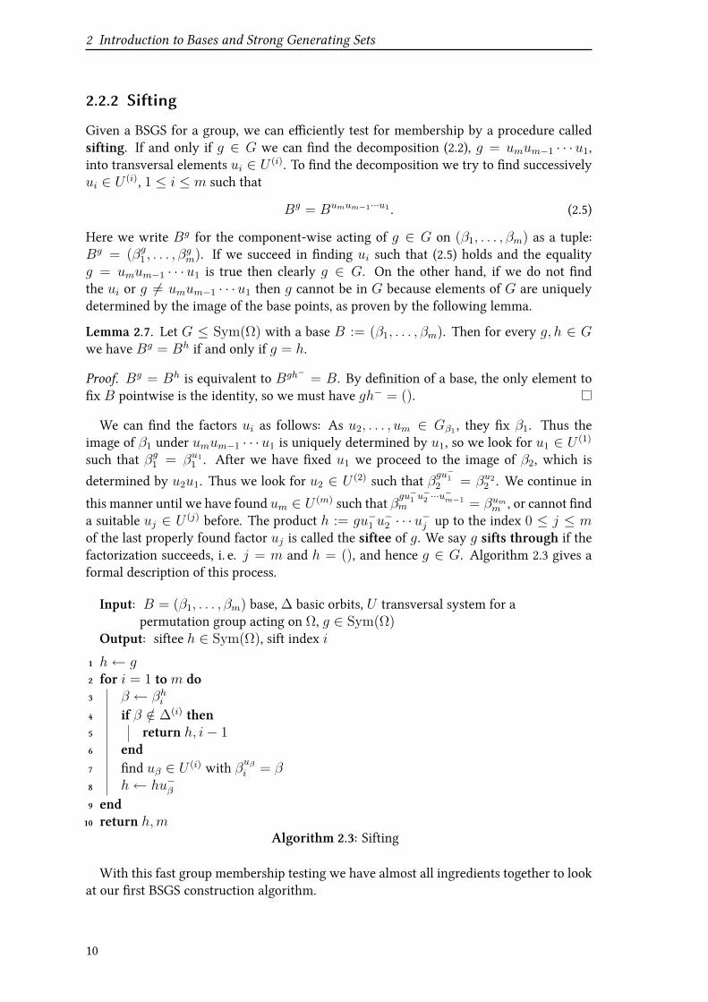
2.2.2 Sifting
Given a BSGS for a group, we can eXciently test for membership by a procedure calledsifting. If and only if g ∈ G we can Vnd the decomposition (2.2), g = umum−1 · · ·u1,into transversal elements ui ∈ U (i). To Vnd the decomposition we try to Vnd successivelyui ∈ U (i), 1 ≤ i ≤ m such that
Bg = Bumum−1···u1 . (2.5)
Here we write Bg for the component-wise acting of g ∈ G on (β1, . . . , βm) as a tuple:Bg = (βg1 , . . . , β
gm). If we succeed in Vnding ui such that (2.5) holds and the equality
g = umum−1 · · ·u1 is true then clearly g ∈ G. On the other hand, if we do not Vndthe ui or g 6= umum−1 · · ·u1 then g cannot be in G because elements of G are uniquelydetermined by the image of the base points, as proven by the following lemma.
Lemma 2.7. Let G ≤ Sym(Ω) with a base B := (β1, . . . , βm). Then for every g, h ∈ Gwe have Bg = Bh if and only if g = h.
Proof. Bg = Bh is equivalent to Bgh− = B. By deVnition of a base, the only element toVx B pointwise is the identity, so we must have gh− = ().
We can Vnd the factors ui as follows: As u2, . . . , um ∈ Gβ1 , they Vx β1. Thus theimage of β1 under umum−1 · · ·u1 is uniquely determined by u1, so we look for u1 ∈ U (1)
such that βg1 = βu11 . After we have Vxed u1 we proceed to the image of β2, which is
determined by u2u1. Thus we look for u2 ∈ U (2) such that βgu−1
2 = βu22 . We continue in
this manner until we have found um ∈ U (m) such that βgu−1 u
−2 ···u
−m−1
m = βumm , or cannot Vnda suitable uj ∈ U (j) before. The product h := gu−1 u
−2 · · ·u−j up to the index 0 ≤ j ≤ m
of the last properly found factor uj is called the siftee of g. We say g sifts through if thefactorization succeeds, i. e. j = m and h = (), and hence g ∈ G. Algorithm 2.3 gives aformal description of this process.
Input: B = (β1, . . . , βm) base, ∆ basic orbits, U transversal system for apermutation group acting on Ω, g ∈ Sym(Ω)
Output: siftee h ∈ Sym(Ω), sift index i
h← g1
for i = 1 tom do2
β ← βhi3
if β /∈ ∆(i) then4
return h, i− 15
end6
Vnd uβ ∈ U (i) with βuβi = β7
h← hu−β8
end9
return h,m10
Algorithm 2.3: Sifting
With this fast group membership testing we have almost all ingredients together to lookat our Vrst BSGS construction algorithm.
10

2.3 BSGS construction with Schreier-Sims algorithm
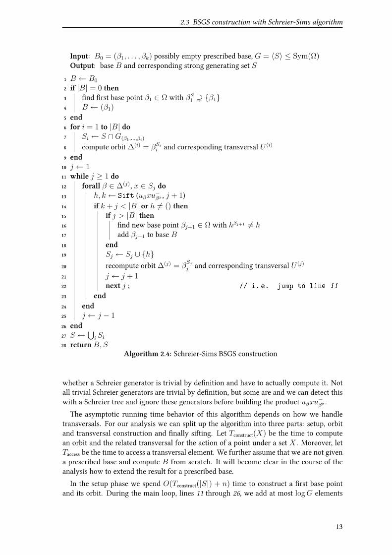
2.3 BSGS construction with Schreier-Sims algorithm
In his paper [Sim70] from 1970 Sims devised a straightforward algorithm to construct aBSGS based on a lemma of Schreier (Lemma 2.8 below). In this section we analyze avariant of this Schreier-Sims algorithm due to [Ser03, Sec. 4.2]. We shall need the followingtwo observations for our analysis. The Vrst lemma presents a way to compute generatorsof a stabilizer. The second lemma gives us a criterion by which we can verify if a givengenerator set is a strong generating set.
Lemma 2.8 (Schreier generators). Let G = 〈X〉 ≤ Sym(Ω) and α ∈ Ω. Let U be atransversal for G modulo Gα and uβ ∈ U be the transversal element mapping α to β.Then
Gα = 〈uβxu−βx : β ∈ αG, x ∈ X〉 (2.6)
We call these generators Schreier generators for Gα.
Proof. It suXces to show that every element h ∈ Gα is generated by T := uβxu−βx :
β ∈ αG, x ∈ X because 〈T 〉 ≤ Gα by deVnition of T . So let h = x1 · · ·xk ∈ Gα withxi ∈ X arbitrary. We now apply a sequence of transformations until h can easily be seento be of the form h = t1 · · · tk, ti ∈ T . Our intermediate elements hj will be of the form
hj = t1 · · · tjuγj+1xj+1xj+2 · · ·xk
We start with h0 := x1 · · ·xk = uαx1 · · ·xk. Given hj , we set tj+1 := uγj+1xj+1u
−γxj+1j+1
and γj+2 := γxj+1
j+1 , ensuring hj+1 = hj = h. We can iterate this process until we reachhk = t1t2 · · · tkuγk+1
. Because hk = h ∈ Gα and (t1t2 · · · tk) ∈ 〈T 〉 ≤ Gα we musthave uγk+1
∈ U ∩ Gα. Since U is a transversal modulo Gα the element uγk+1must be
the identity. Thus we have h in the desired form h = t1t2 · · · tk, showing the inclusionGα ≤ 〈T 〉, hence Gα = 〈T 〉.
Lemma 2.9. Let B := β1, β2, . . . , βm ⊆ Ω and G ≤ Sym(Ω). For 1 ≤ j ≤ m + 1deVne G[j] := G(β1,...,βj−1) as before and let Sj ⊆ G[j] with 〈Sj〉 ≥ 〈Sj+1〉. If 〈S1〉 = G,Sm+1 = ∅, and for 1 ≤ j ≤ m
〈Sj〉βj = 〈Sj+1〉 (2.7)
holds then B is a base for G and S :=⋃j≤m Sj is a strong generating set for G relative to
B.
Proof. We use induction on |Ω|. For |Ω| = 1 we have only () as group generator andnothing more to proof. So let Ω be of arbitrary size n and be the statement of the lemmatrue for |Ω| ≤ n − 1. According to DeVnition 2.3 of an SGS we have to verify thatG[i] = 〈S ∩ G[i]〉 holds for 2 ≤ i ≤ n. We Vrst look at the case i = 2. We obtain from(2.7), with j = 1, and S2 ⊆ G[2] that
Gβ1 = 〈S2〉 = 〈S2 ∩G[2]〉 ≤ 〈S ∩Gβ1〉 ≤ Gβ1 (2.8)
Because the left-most and right-most terms are equal all inner relations are likewise ful-Vlled with equality. Hence (2.4) holds for i = 2.
11

2 Introduction to Bases and Strong Generating Sets
For i > 2 we can apply the lemma to the case B′ = (β2, . . . , βm), S ′ =⋃
2≤j≤m Sj andG′ = Gβ1 so that we have a group acting on n− 1 elements. By doing this, we obtain thatG′(β2,...,βi−1) = 〈S ′ ∩G′(β2,...,βi−1)〉. This implies
G[i] = (Gβ1)(β2,...,βi−1) = 〈S ′ ∩G(β1,...,βi−1)〉 ≤ 〈S ∩G(β1,...,βi−1)〉 ≤ G(β1,...,βi−1) = G[i]
(2.9)So (2.8) and (2.9) show that the SGS condition (2.4) is fulVlled for all i. Thus S is a stronggenerating set relative to the base B.
Finally we are ready to construct a base and strong generating set for G = 〈X〉 withthe Schreier-Sims algorithm. We proceed by extending a list B = (β1, . . . , βk) and sets Sithat approximate a generating set for G[i], maintaining 〈Si〉 ≥ 〈Si+1〉 for all i. We say ourconstruction is up to date above level j when additionally (2.7) holds for all j < i ≤ k.When we are up to date above level 0 it follows from Lemma 2.9 that we have found aBSGS.To start the algorithm we choose a β1 ∈ Ω which is moved by at least one generator in
X . We set B = (β1) and S1 := X and we are up to date above level 1.When we are up to date above level j, we test whether (2.7) holds for i = j. The
inclusion 〈Sj〉βj ≥ 〈Sj+1〉 is always fulVlled by our construction as we ensure that Si ⊆G[i] and hence that βj is invariant under Sj+1. So we need only to test the oppositeinclusion 〈Sj〉βj ≤ 〈Sj+1〉. This can be done by checking that all generators of 〈Sj〉βj liein 〈Sj+1〉.Note that Lemma 2.8 gives a description of the generators of 〈Sj〉βj , which we can use
for testing. Furthermore, Lemma 2.9 ensures that we have an SGS for 〈Sj+1〉, so we cantest membership by sifting.If all Schreier generators of 〈Sj〉βj are in 〈Sj+1〉 and we thus have veriVed (2.7), we are
up to date above level j − 1. Otherwise we have computed a nontrivial siftee h which weadd to Sj+1 and are up to date above level j + 1. In the case j = k we also add a newβk+1 ∈ Ω to our list with hβk+1 6= h.Algorithm 2.4 depicts a more formal description of the process. The call Sift with
parameter j + 1 means we use Algorithm 2.3 on our partial base (βj+1, . . . , β|B|) andpartial strong generating set
⋃i≥j+1 Si because we are testing for membership in Sj+1.
Our Schreier generator sifts through if and only if k ≥ |B| − (j + 1) + 1 and h is theidentity, thus the check in line 14. In an implementation we could slightly improve thisalgorithm by avoiding to sift the same Schreier generator twice when we reach the for-loop at line 12 at a j we have worked at before.Another ineXciency occurs when we use this algorithm with Schreier tree transversals.
Suppose we construct an orbit αS and during its construction create an orbit element βx
from some x ∈ S and a previous element β ∈ αS . Then the Schreier generator g :=uβxu
−βx constructed from β and x is always the identity, g = (). We call these Schreier
generators trivial by deVnition as coined by [HEO05, Sec. 4.1] and we can ignore themin the Schreier-Sims algorithm. However, we are only able to detect Schreier generatorsthat are trivial by deVnition if we use a Schreier tree transversal. In this case, constructinga Schreier generator from the pair (β, x), we know that βx was constructed by x because−−→βx β is an edge of the tree with label x. In the other case of an explicit transversal we haveno history information of how βx ∈ αS was initially constructed. Thus we cannot decide
12
2.3 BSGS construction with Schreier-Sims algorithm
Input: B0 = (β1, . . . , βk) possibly empty prescribed base, G = 〈S〉 ≤ Sym(Ω)Output: base B and corresponding strong generating set S
B ← B01
if |B| = 0 then2
Vnd Vrst base point β1 ∈ Ω with βS1 ) β13
B ← (β1)4
end5
for i = 1 to |B| do6
Si ← S ∩G(β1,...,βi)7
compute orbit ∆(i) = βSii and corresponding transversal U (i)8
end9
j ← 110
while j ≥ 1 do11
forall β ∈ ∆(j), x ∈ Sj do12
h, k ← Sift (uβxu−βx , j + 1)13
if k + j < |B| or h 6= () then14
if j > |B| then15
Vnd new base point βj+1 ∈ Ω with hβj+1 6= h16
add βj+1 to base B17
end18
Sj ← Sj ∪ h19
recompute orbit ∆(j) = βSjj and corresponding transversal U (j)
20
j ← j + 121
next j ; // i. e. jump to line 1122
end23
end24
j ← j − 125
end26
S ←⋃i Si27
return B, S28
Algorithm 2.4: Schreier-Sims BSGS construction
whether a Schreier generator is trivial by deVnition and have to actually compute it. Notall trivial Schreier generators are trivial by deVnition, but some are and we can detect thiswith a Schreier tree and ignore these generators before building the product uβxu−βx .
The asymptotic running time behavior of this algorithm depends on how we handletransversals. For our analysis we can split up the algorithm into three parts: setup, orbitand transversal construction and Vnally sifting. Let Tconstruct(X) be the time to computean orbit and the related transversal for the action of a point under a set X . Moreover, letTaccess be the time to access a transversal element. We further assume that we are not givena prescribed base and compute B from scratch. It will become clear in the course of theanalysis how to extend the result for a prescribed base.
In the setup phase we spend O(Tconstruct(|S|) + n) time to construct a Vrst base pointand its orbit. During the main loop, lines 11 through 26, we add at most logG elements
13
2 Introduction to Bases and Strong Generating Sets
to each set Sj because every time we do this |〈Sj〉| increases. This sums up to a time ofO(|B| log |G|Tconstruct(log |G|) + log |G|Tconstruct(|S|)).For the sifting part, we note that we have to consider each of the
∑j |U (j)||Sj| ∈
O(n log2 |G|+|S|n) Schreier generators only once. Sifting can be done inO(log |G|Taccess)time. So the sifting part sums up to O((n log2 |G|+ |S|n) log |G|Taccess).We can plug in the results from Section 2.2.1, summarized in Figure 2.4 on page 15, for
Taccess and Tconstruct. For explicit transversals we thus need O(n2 log3 |G| + |S|n2 log |G|)time. Choosing Schreier tree transversals results in a O(n3 log3 |G| + |S|n3 log |G|) timecomplexity. Regarding memory usage we note that we always have a O(|S|n) require-ment for the group generators. Additionally, we have to store
∑j |Sj| strong generators
which is O(log2 |G|). By a result of [CST89, Thm. 1], this is also O(n log |G|), even iflog |G| /∈ O(n). For the log |G|many transversals U (j) we need in the explicit case O(n2)memory each and O(n) in the Schreier tree case. Thus the memory requirements sum upto O(n2 log |G|+ |S|n) and O(n log2 |G|+ |S|n), respectively.There are a lot of other BSGS construction algorithms. [But91, Ch. 14] provides a nice
overview of the deterministic algorithms before 1990, which are, roughly speaking, alsoO(n5). All these deterministic algorithms tend to scale badly for groups of large degreebecause there may be a lot of Schreier generators to be constructed, which then have tobe sifted. A practical alternative are randomized constructions with deterministic or ran-domized routines checking for the SGS property. The interested reader may Vnd in [Ser03,Sec. 4.5] a nearly linear-time randomized construction algorithm, which is also imple-mented in GAP. [Ser03, Ch. 8] presents two classical strong generating tests commonlyused in GAP and Magma.
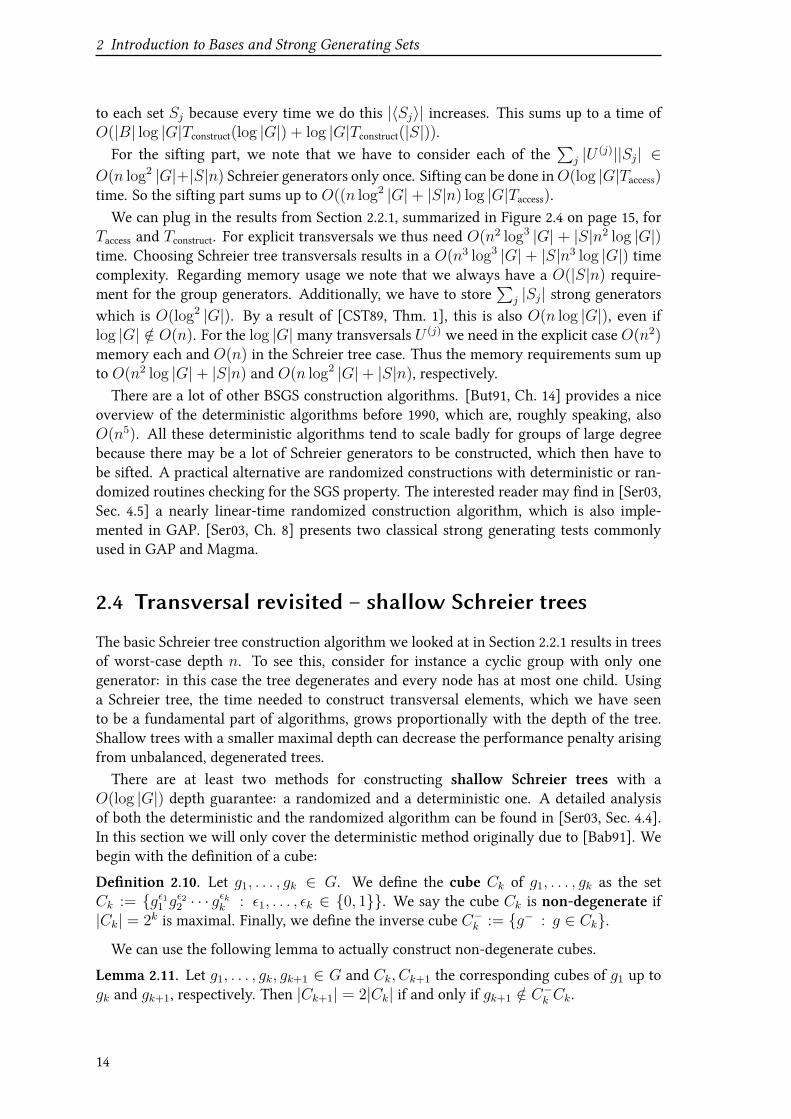
2.4 Transversal revisited – shallow Schreier trees
The basic Schreier tree construction algorithm we looked at in Section 2.2.1 results in treesof worst-case depth n. To see this, consider for instance a cyclic group with only onegenerator: in this case the tree degenerates and every node has at most one child. Usinga Schreier tree, the time needed to construct transversal elements, which we have seento be a fundamental part of algorithms, grows proportionally with the depth of the tree.Shallow trees with a smaller maximal depth can decrease the performance penalty arisingfrom unbalanced, degenerated trees.There are at least two methods for constructing shallow Schreier trees with a
O(log |G|) depth guarantee: a randomized and a deterministic one. A detailed analysisof both the deterministic and the randomized algorithm can be found in [Ser03, Sec. 4.4].In this section we will only cover the deterministic method originally due to [Bab91]. Webegin with the deVnition of a cube:
DeVnition 2.10. Let g1, . . . , gk ∈ G. We deVne the cube Ck of g1, . . . , gk as the setCk := gε11 g
ε22 · · · g
εkk : ε1, . . . , εk ∈ 0, 1. We say the cube Ck is non-degenerate if
|Ck| = 2k is maximal. Finally, we deVne the inverse cube C−k := g− : g ∈ Ck.
We can use the following lemma to actually construct non-degenerate cubes.
Lemma 2.11. Let g1, . . . , gk, gk+1 ∈ G and Ck, Ck+1 the corresponding cubes of g1 up togk and gk+1, respectively. Then |Ck+1| = 2|Ck| if and only if gk+1 /∈ C−k Ck.
14
2.4 Transversal revisited – shallow Schreier trees
Proof. |Ck+1| = 2|Ck| is equivalent to the fact that the sets Ck and Ckgk+1 are disjoint.They are disjoint if and only if gk+1 /∈ C−k Ck.
So for the construction of a non-degenerate cube Ck we iteratively construct cubes Ci+1
from Ci such that gi+1 /∈ C−i Ci. Membership testing in C−i Ci in general is diXcult (cf.[Ser03, p. 65]), but for our purposes an easier to compute condition for non-membership issuXcient. Clearly, if, for some α ∈ Ω, we Vnd a g ∈ G with αg /∈ αC−i Ci , then g /∈ C−i Ci.We can compute the set αC
−k Ck iteratively in O(kn) time. Beginning with ∆1 :=
α, we set ∆i+1 := ∆i ∪ ∆hii where hi is the i-th member of the sequence
g−k , g−k−1, . . . , g
−1 , g1, g2, . . . , gk. This induces a directed, labeled graph on the vertex set
αC−k Ck with label set hi : 1 ≤ i ≤ 2k = g−i , gi : 1 ≤ i ≤ k. In this a graph an edge
−−−→α1 α2 exists and has label h−i , if α1 = αhi2 for some i. A breadth-Vrst-search on this graphyields a Schreier tree as in DeVnition 2.5.
Suppose we have a non-degenerate cube Ck of g1, . . . , gk ∈ G with αC−k Ck = αG. The
non-degeneracy of the cube ensures k ≤ log |G|, thus the Schreier tree constructed asabove has depth at most 2 · k ≤ 2 log |G|.It remains to be discussed how we can construct the mentioned cube Ck with αC
−k Ck =
αG. To this end, we Vnd a Vrst element g1 that moves α. Especially g1 6= (), so C1 isnon-degenerate. If αC
−1 C1 = αG we are done. If this is not the case then we Vnd an s ∈ G
with αs /∈ αC−1 C1 and set g2 := s. We then have an extended non-degenerate cube C2
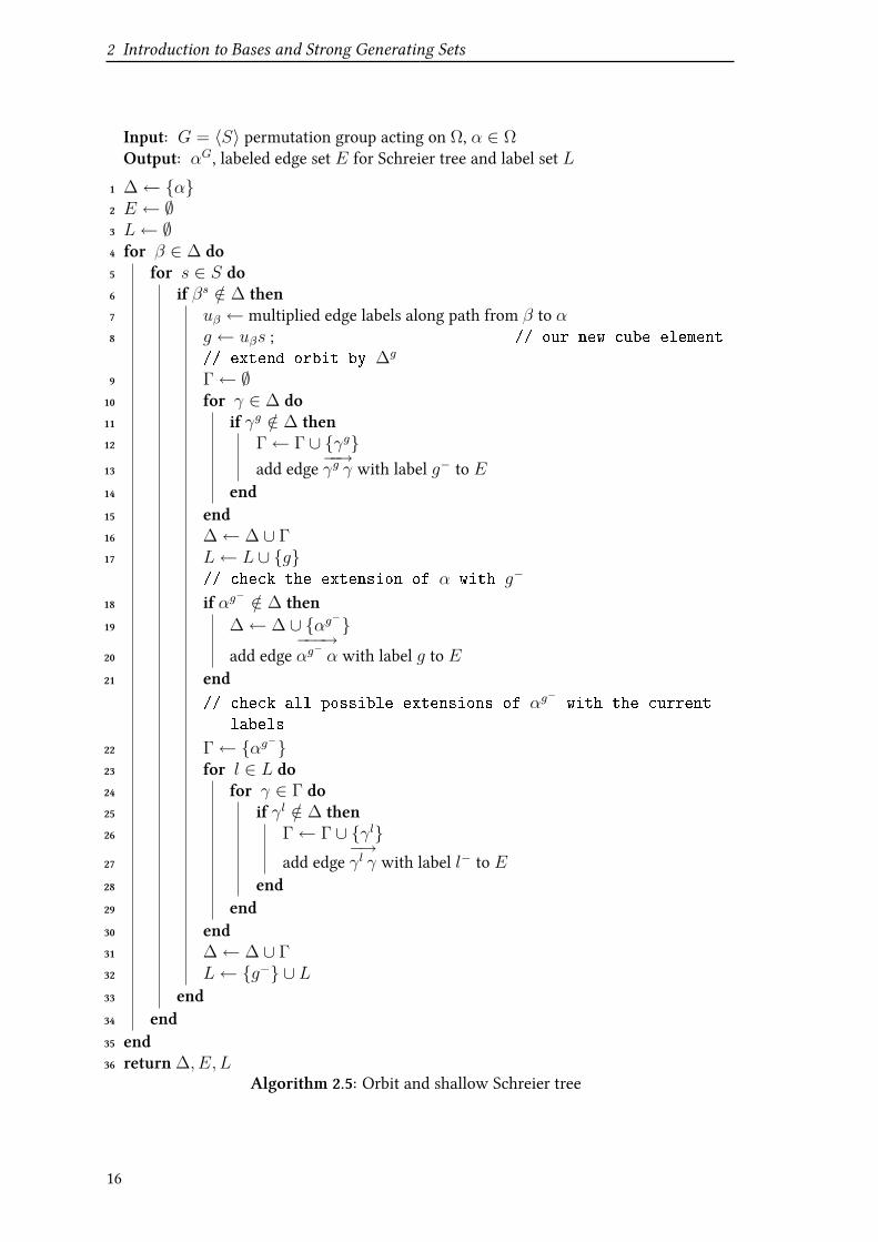
which either suXces to generate the orbit or we Vnd another group element to extend thecube.Algorithm 2.5 has the details. What makes it rather long compared to the idea described
above is to avoid repeating checks for αC−i Ci when working on αC
−i+1Ci+1 . Therefore, when
we have a new cube element g in line 8, we Vrst compute αC−i Cig in lines 9 to 16 and then
αg−C−i Ci+1 in lines 18 to 31. Furthermore, important to note is that we treat L as an ordered
set so that we insert g at the end (l. 17) and g− at the front (l. 32) of the label sequence.Constructing a shallow variant of a Schreier tree costs extra time. As in every orbit
computation we always need O(|S|n) by the two for-loops in lines 4 and 5 of Algorithm2.5. Besides that, we also have to deal with cubes. As we have seen before, for every i ≤ k
the set αC−i Ci can be computed inO(nk) time, which we have to construct at most k times.
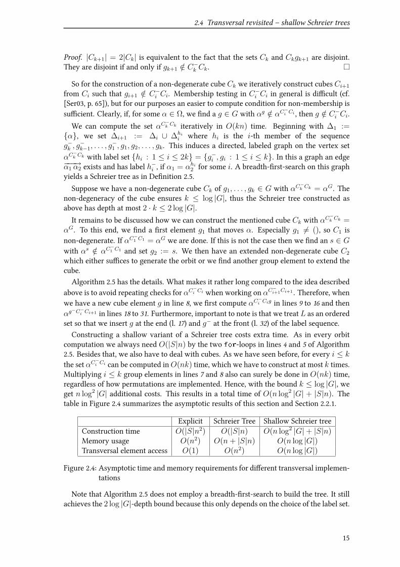
Multiplying i ≤ k group elements in lines 7 and 8 also can surely be done in O(nk) time,regardless of how permutations are implemented. Hence, with the bound k ≤ log |G|, weget n log2 |G| additional costs. This results in a total time of O(n log2 |G| + |S|n). Thetable in Figure 2.4 summarizes the asymptotic results of this section and Section 2.2.1.
Explicit Schreier Tree Shallow Schreier treeConstruction time O(|S|n2) O(|S|n) O(n log2 |G|+ |S|n)Memory usage O(n2) O(n+ |S|n) O(n log |G|)Transversal element access O(1) O(n2) O(n log |G|)
Figure 2.4: Asymptotic time and memory requirements for diUerent transversal implemen-tations
Note that Algorithm 2.5 does not employ a breadth-Vrst-search to build the tree. It stillachieves the 2 log |G|-depth bound because this only depends on the choice of the label set.
15
2 Introduction to Bases and Strong Generating Sets
Input: G = 〈S〉 permutation group acting on Ω, α ∈ ΩOutput: αG, labeled edge set E for Schreier tree and label set L
∆← α1
E ← ∅2
L← ∅3
for β ∈ ∆ do4
for s ∈ S do5
if βs /∈ ∆ then6
uβ ← multiplied edge labels along path from β to α7
g ← uβs ; // our new cube element8
// extend orbit by ∆g
Γ← ∅9
for γ ∈ ∆ do10
if γg /∈ ∆ then11
Γ← Γ ∪ γg12
add edge−−→γg γ with label g− to E13
end14
end15
∆← ∆ ∪ Γ16
L← L ∪ g17
// check the extension of α with g−
if αg−/∈ ∆ then18
∆← ∆ ∪ αg−19
add edge−−−→αg−α with label g to E20
end21
// check all possible extensions of αg−
with the current
labels
Γ← αg−22
for l ∈ L do23
for γ ∈ Γ do24
if γl /∈ ∆ then25
Γ← Γ ∪ γl26
add edge−→γl γ with label l− to E27
end28
end29
end30
∆← ∆ ∪ Γ31
L← g− ∪ L32
end33
end34
end35
return ∆, E, L36
Algorithm 2.5: Orbit and shallow Schreier tree
16

2.5 Base change
A breadth-Vrst-approach, however, will produce trees of lesser or equal depth on the sameinput. For an implementation of this improvement we would have to keep track of thedepth d(α) of orbit elements α ∈ ∆ in the already constructed part of the tree. A bucketsort (cf. [CLRS09, Sec. 8.4]) with respect to d(α), providing insertion into a d(α)-sortedsequence in O(1) time, could be used without deteriorating the asymptotic time behaviorgiven above.
2.5 Base change
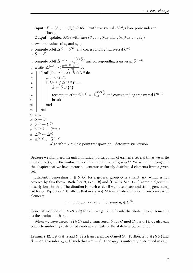
As we will see later, many applications that rely on computations with bases and stronggenerating sets require a speciVc base. For example, if we want to compute stabilizers (cf.Section 3.1.4) then we need a base which is closely related to the set we like to stabilize.Because constructing a complete BSGS from scratch is likely to be an expensive processwe would like to have an algorithm that modiVes a strong generating set with respect tobase (β1, . . . , βm) so that it is strong generating relative to some other base (α1, . . . , αk).In this section we will examine several solutions to this problem. The interested readermay also Vnd several of the presented algorithms with examples in [But91, Ch. 12] and[Ser03, Sec. 5.4].Assume for a moment that we know how to perform a base point transposition. Given
an SGS relative to a base (β1, . . . , βm), a base point transposition at i constructs an SGSrelative to (β1, . . . , βi−1, βi+1, βi, βi+2, βi+3, . . . , βm). We can use this method to insert anew base point α ∈ Ω at a speciVc position j ≤ m. First we insert α as a redundant basepoint after the Vrst βi such that G[i+1] = G(β1,...,βi) Vxes α. This ensures that G(β1,...,βi) =G(β1,...,βi,α) and the new transversal that we insert is trivial. Then we apply |i − j| manytranspositions to bring α into the desired position, which gives us a possibly redundantbase (β1, . . . , βj−1, α, βj, . . . , βm). Note that if i < j all necessary transpositions aretrivial and we can also insert α directly at position j. By repeating such insertions withα1 at position 1, α2 at position 2 &c., and stripping redundant elements afterward, we canchange the base to a completely diUerent one (α1, α2, . . . , αk−1, αk, . . . ).Algorithm 2.6 formalizes this base change procedure. The following two sections present
two algorithms, one deterministic, one randomized, to perform a base point transposition.
2.5.1 Deterministic base point transposition
The Vrst, deterministic transposition algorithm is due to Sims (cf. [Sim71b]). Let S bean SGS for G relative to the base (β1, . . . , βm) with stabilizer chain G = G[1] ≥ · · · ≥G[m] ≥ G[m+1] = 1 and transversals U (1), . . . , U (m). Our goal is to compute an SGS Srelative to (β1, . . . , βi−1, βi+1, βi, . . . , βm) with stabilizer chainG = G[1] ≥ · · · ≥ G[m] ≥G[m+1] = 1 and transversals U (1), . . . , U (m).Most of the stabilizers do not change, we have G[j] = G[j] for every j 6= i + 1. Ac-
cordingly for 1 ≤ j < i and i + 1 < j ≤ m the transversals do not change, U (j) = U (j).We can easily compute the new i-th fundamental orbit βG
[i]
i+1 and obtain a new transversalU (i). It remains to set up U (i+1).As we do not know a generating set for G[i+1] yet we iteratively construct the new
(i + 1)-st fundamental orbit ∆(i+1), starting with ∆(i+1) := βi and S := S. Then we
17

2 Introduction to Bases and Strong Generating Sets
Input: B = (β1, . . . , βm), S BSGS, sequence of new base points (α1, . . . , αk)Output: updated BSGS with base (α1, . . . , αk, . . . )
for i = 1 to k do1
if βi 6= αi then2
// find insertion position
j ← i+ 13
while αG[j+1]
i ) αi do4
j ← j + 15
end6
insert αi into B at position j7
insert ∆(i) = αi and corresponding transversal U (i) into sequence of orbits8
and transversals at position jwhile j > i do9
B, S ← Transpose (B, S, j − 1)10
j ← j − 111
end12
end13
end14
Algorithm 2.6: Base change with transpositions
construct Schreier generators from U (i) and G[i]. Whenever we Vnd a Schreier generatorh ∈ G[i+1] that extends our orbit, we add h to S. With the new generator we recompute
∆(i+1) := β〈S∩G[i+1]〉i = β
〈S∩G[i]βi+1
〉i . From |G| =
∏mi=1 |U (i)| by (2.3) we know that for the
Vnal orbit we must have
|∆(i+1)| = |U (i+1)| = |U(i+1)| · |U (i)||U (i)|
.
If the number of elements in ∆(i+1) is below that number, we proceed with anotherSchreier generator. In the case we have reached this cardinality for ∆(i+1), we knowthat we have a complete generating set for G[i+1] and, along with our orbit calculations,a transversal U (i+1) and so we are done. As in the Schreier-Sims algorithm in Section 2.3,for performance reasons we should avoid constructing Schreier generators that are trivialby deVnition.
Algorithm 2.7 shows an in-place variant of the transposition part. Again, like in theSchreier-Sims construction, it would be an improvement for an implementation to con-struct and check each Schreier generator in line 6 only once. A detailed analysis in [But91,p. 123] shows that this deterministic base point transposition has a O(n4) complexity.
2.5.2 Randomized base point transposition
Random group elements
Instead of computing Schreier generators for G[i+1] explicitly, we can use randomness.But Vrst of all we need to know how to eXciently construct random elements of a group.
18
2.5 Base change
Input: B = (β1, . . . , βm), S BSGS with transversals U (j), i base point index tochange
Output: updated BSGS with base (β1, . . . , βi−1, βi+1, βi, βi+2, . . . , βm)
swap the values of βi and βi+11
compute orbit ∆(i) = βG[i]
i and corresponding transversal U (i)2
S ← S3
compute orbit ∆(i+1) = β〈S∩G[i]
βi〉
i+1 and corresponding transversal U (i+1)4
while |∆(i+1)| < |U(i+1)|·|U(i)||U(i)| do5
forall β ∈ ∆(i), x ∈ S ∩G[i] do6
h← uβxu−βx7
if hβi+1 /∈ ∆(i+1) then8
S ← S ∪ h9
recompute orbit ∆(i+1) = β〈S∩G[i]
βi〉
i+1 and corresponding transversal U (i+1)10
break11
end12
end13
end14
S ← S15
U (i) ← U (i)16
U (i+1) ← U (i+1)17
∆(i) ← ∆(i)18
∆(i+1) ← ∆(i+1)19
Algorithm 2.7: Base point transposition – deterministic version
Because we shall need the uniform random distribution of elements several times we writein short U(G) for the uniform distribution on the set or group G. We assume throughoutthe chapter that we have means to generate uniformly distributed elements from a givenset.
EXciently generating g ∈ U(G) for a general group G is a hard task, which is notcovered by this thesis. Both [Ser03, Sec. 2.2] and [HEO05, Sec. 3.2.2] contain algorithmdescriptions for that. The situation is much easier if we have a base and strong generatingset for G. Equation (2.2) tells us that every g ∈ G is uniquely composed from transversalelements
g = umum−1 · · ·u2u1, for some ui ∈ U (i).
Hence, if we choose ui ∈ U(U (i)) for all i we get a uniformly distributed group element gas the product of the ui.
When we have access to U(G) and a transversal U for G mod Gα, α ∈ Ω, we also cancompute uniformly distributed random elements of the stabilizer Gα as follows:
Lemma 2.12. Let α ∈ Ω and U be a transversal for G mod Gα. Further, let g ∈ U(G) andβ := αg. Consider uβ ∈ U such that αuβ = β. Then gu−β is uniformly distributed in Gα.
19
2 Introduction to Bases and Strong Generating Sets
Proof. Let u1, . . . , uk =: U be the transversal elements. Then G can be partitioned inG =
⋃ki=1Gαui. Every g ∈ G is in exactly one coset Gαuβ . So every coset Gαui has the
same chance to occur as Gαuβ and every h ∈ Gα has the same chance to occur as gu−β .Thus gu−β is uniformly distributed in Gα if g is uniformly distributed in G.
Transposition
For a base transposition we are in the situation that we know G[i] and have a transversalU (i) for G[i] mod G[i+1]. We then need generators for G[i+1] = G
[i]βi+1
. So instead ofcomputing Schreier generators, we generate g ∈ U(G[i+1]) according to Lemma 2.12 fromU (i) and G[i] = G[i], which we already have an SGS for. Then we test whether g extendsthe known transversal part. If it does then we add it to our generating set and start overagain.
Input: B = (β1, . . . , βm), S BSGS with transversals U (j), i base point index tochange
Output: updated BSGS with base (β1, . . . , βi−1, βi+1, βi, βi+2, . . . , βm)
swap the values of βi and βi+11
compute orbit ∆(i) = βG[i]
i and corresponding transversal U (i)2
S ← S3
compute orbit ∆(i+1) = β〈S∩G[i]
βi〉
i+1 and corresponding transversal U (i+1)4
while |∆(i+1)| < |U(i+1)|·|U(i)||U(i)| do5
generate g ∈ U(G[i])6
Vnd ug ∈ U (i) with βugi+1 = βgi+17
h← gu−g8
if hβi+1 /∈ ∆(i+1) then9
S ← S ∪ h10
recompute orbit ∆(i+1) = β〈S∩G[i]
βi〉
i+1 and corresponding transversal U (i+1)11
end12
end13
S ← S14
U (i) ← U (i)15
U (i+1) ← U (i+1)16
∆(i) ← ∆(i)17
∆(i+1) ← ∆(i+1)18
Algorithm 2.8: Base point transposition – randomized version
One can prove that, if S is not complete then with probability of at least 12such ran-
domly generated g will not sift through our partial BSGS and therefore extend our gener-ating set (cf. [Ser03, Lemma 4.3.1]). Also note that because we know the size of the newtransversal U (i+1) in advance we know when we have found enough generators to makeS a strong generating set. Hence we have a randomized base transposition algorithm andwe can tell whether its result is correct by looking at the size of the transversal product.
20
2.5 Base change
Algorithm 2.8 formalizes the process and is very similar to the deterministic version inAlgorithm 2.7. The only diUerence is how we Vnd the probable generators h. Note thatbecause of the randomized nature of this algorithm we cannot guarantee its termination.
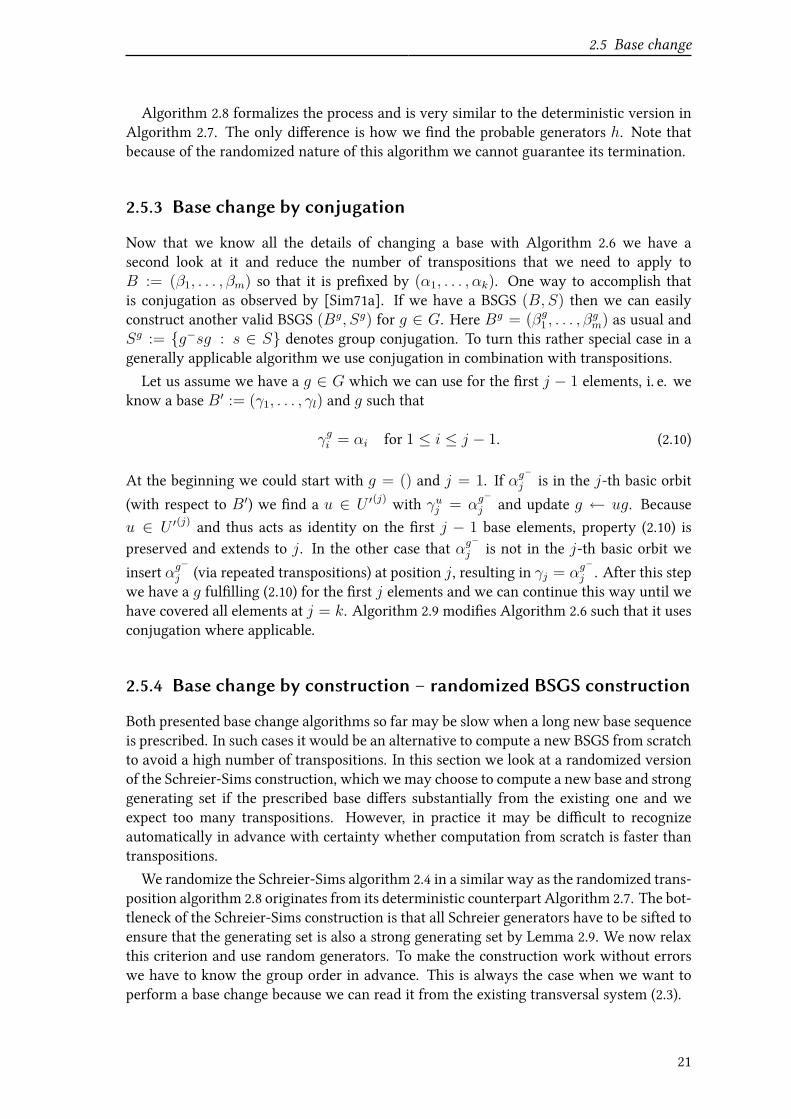
2.5.3 Base change by conjugation
Now that we know all the details of changing a base with Algorithm 2.6 we have asecond look at it and reduce the number of transpositions that we need to apply toB := (β1, . . . , βm) so that it is preVxed by (α1, . . . , αk). One way to accomplish thatis conjugation as observed by [Sim71a]. If we have a BSGS (B, S) then we can easilyconstruct another valid BSGS (Bg, Sg) for g ∈ G. Here Bg = (βg1 , . . . , β
gm) as usual and
Sg := g−sg : s ∈ S denotes group conjugation. To turn this rather special case in agenerally applicable algorithm we use conjugation in combination with transpositions.
Let us assume we have a g ∈ G which we can use for the Vrst j − 1 elements, i. e. weknow a base B′ := (γ1, . . . , γl) and g such that
γgi = αi for 1 ≤ i ≤ j − 1. (2.10)
At the beginning we could start with g = () and j = 1. If αg−
j is in the j-th basic orbit
(with respect to B′) we Vnd a u ∈ U ′(j) with γuj = αg−
j and update g ← ug. Because
u ∈ U ′(j) and thus acts as identity on the Vrst j − 1 base elements, property (2.10) ispreserved and extends to j. In the other case that αg
−
j is not in the j-th basic orbit we
insert αg−
j (via repeated transpositions) at position j, resulting in γj = αg−
j . After this stepwe have a g fulVlling (2.10) for the Vrst j elements and we can continue this way until wehave covered all elements at j = k. Algorithm 2.9 modiVes Algorithm 2.6 such that it usesconjugation where applicable.
2.5.4 Base change by construction – randomized BSGS construction
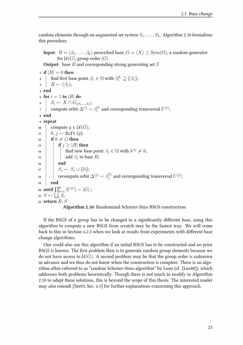
Both presented base change algorithms so far may be slow when a long new base sequenceis prescribed. In such cases it would be an alternative to compute a new BSGS from scratchto avoid a high number of transpositions. In this section we look at a randomized versionof the Schreier-Sims construction, which we may choose to compute a new base and stronggenerating set if the prescribed base diUers substantially from the existing one and weexpect too many transpositions. However, in practice it may be diXcult to recognizeautomatically in advance with certainty whether computation from scratch is faster thantranspositions.
We randomize the Schreier-Sims algorithm 2.4 in a similar way as the randomized trans-position algorithm 2.8 originates from its deterministic counterpart Algorithm 2.7. The bot-tleneck of the Schreier-Sims construction is that all Schreier generators have to be sifted toensure that the generating set is also a strong generating set by Lemma 2.9. We now relaxthis criterion and use random generators. To make the construction work without errorswe have to know the group order in advance. This is always the case when we want toperform a base change because we can read it from the existing transversal system (2.3).
21

2 Introduction to Bases and Strong Generating Sets
Input: B = (β1, . . . , βm), S BSGS, sequence of new base points (α1, . . . , αk)Output: updated BSGS with base (α1, . . . , αk, . . . )
g ← ();1
for i = 1 to k do2
αi ← αg−
i ;3
if βi 6= αi then4
if αi ∈ ∆(i) then5
Vnd element uαi ∈ U (i) such that βuαii = αi;6
g ← uαig;7
else8
// find insertion position
j ← i+ 1;9
while αG[j+1]
i ) αi do10
j ← j + 1;11
end12
insert αi into B as position j;13
insert ∆(i) = αi and corresponding transversal U (i) into sequence of14
orbits and transversals;while j > i do15
B, S ← Transpose (B, S, j − 1);16
j ← j − 1;17
end18
end19
end20
end21
B ← Bg;22
S ← Sg;23
for i = 1 to k do24
recompute orbit ∆(i) and corresponding transversal U (i);25
end26
Algorithm 2.9: Base change with conjugation and transpositions
To construct a base and strong generating set B, S in a randomized fashion for a groupG = 〈X〉, we start similarly to the deterministic Schreier-Sims algorithm. At the begin-ning we choose a β1 ∈ Ω which is moved by at least one generator and start withB = (β1)and S1 := X . If we have a prescribed base we of course skip this step. Let us assume wealready have constructed some subsets S1, . . . , Sk, generating subsets of G[1], . . . , G[k].
We generate uniformly independently distributed random elements g ∈ U(G) accord-ing to the results of Section 2.5.2. We then sift them through the existing transversalsystem. If one of these g does not sift through we end up with an index j and a siftee h.We can add this siftee h to Sj to improve our approximation of a strong generating set.If j = k we also add a new base point βk+1. When the product
∏ki=1 |U (i)| equals the
known base order we are done because no element g ∈ G can have a non-trivial sifteewithout enlarging the transversal product. If the orders mismatch we start again sifting
22
2.5 Base change
random elements through an augmented set system S1, . . . , Sk. Algorithm 2.10 formalizesthis procedure.
Input: B = (β1, . . . , βk) prescribed base, G = 〈X〉 ≤ Sym(Ω), a random generatorfor U(G), group order |G|
Output: base B and corresponding strong generating set S
if |B| = 0 then1
Vnd Vrst base point β1 ∈ Ω with βX1 ) β1;2
B ← (β1);3
end4
for i = 1 to |B| do5
Si ← X ∩G(β1,...,βi);6
compute orbit ∆(i) = βSii and corresponding transversal U (i);7
end8
repeat9
compute g ∈ U(G);10
h, j ← Sift (g);11
if h 6= () then12
if j ≥ |B| then13
Vnd new base point βj ∈ Ω with hβj 6= h;14
add βj to base B;15
end16
Sj ← Sj ∪ h;17
recompute orbit ∆(j) = βSjj and corresponding transversal U (j);18
end19
until∏k
i=1 |U (i)| = |G| ;20
S ←⋃i Si21
return B, S22
Algorithm 2.10: Randomized Schreier-Sims BSGS construction
If the BSGS of a group has to be changed to a signiVcantly diUerent base, using thisalgorithm to compute a new BSGS from scratch may be the fastest way. We will comeback to this in Section 4.2.3 when we look at results from experiments with diUerent basechange algorithms.One could also use this algorithm if an initial BSGS has to be constructed and no prior
BSGS is known. The Vrst problem then is to generate random group elements because wedo not have access to U(G). A second problem may be that the group order is unknownin advance and we thus do not know when the construction is complete. There is an algo-rithm often referred to as “random Schreier-Sims algorithm” by Leon (cf. [Leo80]), whichaddresses both problems heuristically. Though there is not much to modify in Algorithm2.10 to adapt these solutions, this is beyond the scope of this thesis. The interested readermay also consult [Ser03, Sec. 4.3] for further explanations concerning this approach.
23

2 Introduction to Bases and Strong Generating Sets
24
3 Backtrack Search
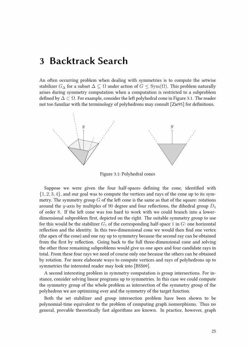
An often occurring problem when dealing with symmetries is to compute the setwisestabilizer G∆ for a subset ∆ ⊆ Ω under action of G ≤ Sym(Ω). This problem naturallyarises during symmetry computation when a computation is restricted to a subproblemdeVned by ∆ ⊂ Ω. For example, consider the left polyhedral cone in Figure 3.1. The readernot too familiar with the terminology of polyhedrons may consult [Zie95] for deVnitions.
y y
Figure 3.1: Polyhedral cones
Suppose we were given the four half-spaces deVning the cone, identiVed with1, 2, 3, 4, and our goal was to compute the vertices and rays of the cone up to its sym-metry. The symmetry group G of the left cone is the same as that of the square: rotationsaround the y-axis by multiples of 90 degree and four reWections, the dihedral group D4
of order 8. If the left cone was too hard to work with we could branch into a lower-dimensional subproblem Vrst, depicted on the right. The suitable symmetry group to usefor this would be the stabilizer G1 of the corresponding half-space 1 in G: one horizontalreWection and the identity. In this two-dimensional cone we would then Vnd one vertex(the apex of the cone) and one ray up to symmetry because the second ray can be obtainedfrom the Vrst by reWection. Going back to the full three-dimensional cone and solvingthe other three remaining subproblems would give us one apex and four candidate rays intotal. From these four rays we need of course only one because the others can be obtainedby rotation. For more elaborate ways to compute vertices and rays of polyhedrons up tosymmetries the interested reader may look into [BSS09].
A second interesting problem in symmetry computation is group intersections. For in-stance, consider solving linear programs up to symmetries. In this case we could computethe symmetry group of the whole problem as intersection of the symmetry group of thepolyhedron we are optimizing over and the symmetry of the target function.
Both the set stabilizer and group intersection problem have been shown to bepolynomial-time equivalent to the problem of computing graph isomorphisms. Thus nogeneral, provable theoretically fast algorithms are known. In practice, however, graph
25
3 Backtrack Search
isomorphisms can often be computed eXciently, despite the unknown complexity classmembership in P (cf. [Luk93]). Like graph isomorphisms, those group problems are usu-ally solved with a backtracking approach. An algorithm walks through the group and Vndsall elements with the desired properties, in this case generating a set stabilizer or a groupintersection. In this section we will study two BSGS-based algorithms for this task, one ofthem inspired by graph isomorphism techniques. These backtracking algorithms are fairlygeneral and also commonly used for other group-theoretic problems like centralizers andnormalizers, which we exclude from our considerations here.
In a general setting, we attempt to Vnd the set G(P) of all elements of a group G sat-isfying a mathematical property P . It seems reasonable that for “unstructured” propertieslike an arbitrary equation in group elements the search has to “touch” almost every singlegroup element. One kind of structure that helps in bounding the search space is thatG(P)is a subgroup ofG or a coset of a subgroup (or empty). In this case search problems usuallybecome tractable despite a worst-case complexity of Ω(|G|).We can also use these subgroup search methods to compute automorphisms of combi-
natorial objects such as matrices. For instance, for a matrix A we may set G := Sym(A)as the group of all permutations acting on A and deVne P to be to true for a g ∈ G if andonly Ag = A. Then G(P) is the automorphisms group of all matrices. To compute G(P)the backtrack framework may remain the same in general, only P speciVc componentshave to be adapted.
For every subgroup problem there is a related coset problem where we would like toVnd one representative of the coset. For instance, consider the set stabilizer problem. Thesubgroup task is to Vnd the setwise stabilizerG∆ for a set ∆ ⊆ Ω. The corresponding cosetproblem is, given Γ,∆ ⊆ Ω, to Vnd g ∈ G with ∆g = Γ (or establish that no such elementexists). In other words, we have to Vnd a representative of a coset (G∆)g with ∆(G∆)g = Γor a representative of a coset g(GΓ) with ∆g(GΓ) = Γ, if such a coset exists. We could thensolve the corresponding subgroup problem to obtain the full coset if it is required, butusually one representative is enough. Going back to the example of a polyhedral cone inFigure 3.1, we need to solve such a coset problem if we want to know whether two verticesor rays Γ,∆ can be obtained from each other by action of the symmetry group G.
To illustrate the methods and techniques we will focus on subgroup search. At the endof each section we will discuss what changes are necessary to perform a search for cosetrepresentatives.
3.1 Classical backtracking
We organize the search forG(P) based on the concept of a search tree which hasG as rootand all elements of G as leaves. We traverse this tree depth-Vrst in search for elementsfulVlling the property P . While doing that, we hope that we can prune whole subtreesbecause they contain irrelevant data to construct G(P). Our goal is to examine as fewleaves (group elements) as possible.
26

3.1 Classical backtracking
3.1.1 Search tree
A base together with a strong generating set enables us to enumerate all group elementsby enumerating all possible transversal combinations
unun−1 · · ·u2u1 with ui ∈ U (i), (3.1)
which is our equation (2.2) from page 6. During this enumeration we can check everyunun−1 · · ·u2u1 if it is in G(P). The key to fast results is a clever organization of thesearch. Thus we set up our search tree in the following way.
DeVnition 3.1. Let B = (β1, . . . , βm) be a base for G with strong generating set S andcorresponding transversals U (i) for 1 ≤ i ≤ m. Our search tree is a labeled tree with thefollowing properties:• The root at level 0 has the empty label ().
• We label every node at level i > 0 with a sequence (γ1, . . . , γi) ∈ Ωi for 1 ≤ i ≤ m.
• A node (γ1, . . . , γi) at level i < m has the children (γ1, . . . , γi, γi+1) for eachγi+1 ∈ (∆(i+1))g where g ∈ G is an arbitrary permutation fulVlling (β1, . . . , βi)
g =(γ1, . . . , γi).
This is just a reformulation of the enumeration based on (3.1). We observe that fromone node of the search tree to one of its children we Vx one more base point image.The parent node has (β1, . . . , βi)
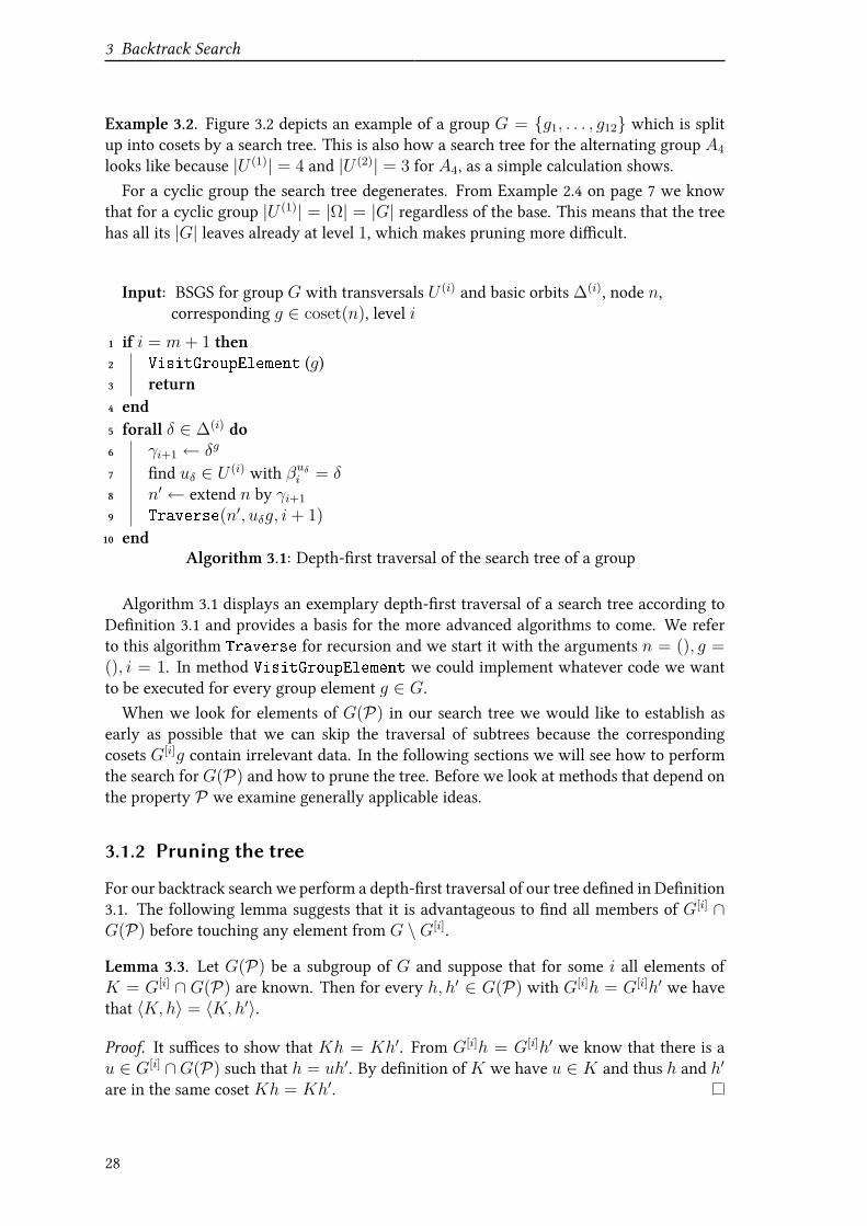
g = (γ1, . . . , γi) for some g ∈ G, the child node has(β1, . . . , βi, βi+1)h = (γ1, . . . , γi, γi+1) for some h ∈ H . We apply the decomposition (3.1)to g = un · · ·u1 and h = vn · · · v1 where uj, vj ∈ U (j). Because of the i Vxed Vrst basepoints we must have that uj = vj for all 1 ≤ j ≤ i. So each path from the root to a leafrepresents a sequence of group elements (u1), (u2u1), (u3u2u1), . . . , (unun−1 · · ·u2u1).This also means that each tree node at level i represents a coset G[i+1]g of G. Al-
though we label the tree with partial base images it is sometimes more convenient tolook at a node as a coset, so we will use the notation that is best in the context. Moreformally, for a node n := (γ1, . . . , γi) we deVne the function coset to return the cor-responding coset: coset(n) = g ∈ G : βgj = γj ∀1 ≤ j ≤ i. The leaves,(γ1, . . . , γm) = (β1, . . . , βm)umum−1···u1 for some uj ∈ U (j), correspond uniquely to groupelements umum−1 · · ·u1 ∈ G. Conversely, because of the way we deVne child nodes,every g = umum−1 · · ·u1 ∈ G corresponds to a leaf (γ1, . . . , γm) = (β1, . . . , βm)g.
G = G[1]
G[2]gi1
g1 g2 g3
G[2]gi2
g4 g5 g6
G[2]gi3
g7 g8 g9
G[2]gi4
g10 g11 g12
Figure 3.2: Group with twelve elements split up into cosets by a search tree
27
3 Backtrack Search
Example 3.2. Figure 3.2 depicts an example of a group G = g1, . . . , g12 which is splitup into cosets by a search tree. This is also how a search tree for the alternating group A4
looks like because |U (1)| = 4 and |U (2)| = 3 for A4, as a simple calculation shows.
For a cyclic group the search tree degenerates. From Example 2.4 on page 7 we knowthat for a cyclic group |U (1)| = |Ω| = |G| regardless of the base. This means that the treehas all its |G| leaves already at level 1, which makes pruning more diXcult.
Input: BSGS for group G with transversals U (i) and basic orbits ∆(i), node n,corresponding g ∈ coset(n), level i
if i = m+ 1 then1
VisitGroupElement (g)2
return3
end4
forall δ ∈ ∆(i) do5
γi+1 ← δg6
Vnd uδ ∈ U (i) with βuδi = δ7
n′ ← extend n by γi+18
Traverse(n′, uδg, i+ 1)9
end10
Algorithm 3.1: Depth-Vrst traversal of the search tree of a group
Algorithm 3.1 displays an exemplary depth-Vrst traversal of a search tree according toDeVnition 3.1 and provides a basis for the more advanced algorithms to come. We referto this algorithm Traverse for recursion and we start it with the arguments n = (), g =(), i = 1. In method VisitGroupElement we could implement whatever code we wantto be executed for every group element g ∈ G.When we look for elements of G(P) in our search tree we would like to establish as
early as possible that we can skip the traversal of subtrees because the correspondingcosets G[i]g contain irrelevant data. In the following sections we will see how to performthe search forG(P) and how to prune the tree. Before we look at methods that depend onthe property P we examine generally applicable ideas.
3.1.2 Pruning the tree
For our backtrack search we perform a depth-Vrst traversal of our tree deVned in DeVnition3.1. The following lemma suggests that it is advantageous to Vnd all members of G[i] ∩G(P) before touching any element from G \G[i].
Lemma 3.3. Let G(P) be a subgroup of G and suppose that for some i all elements ofK = G[i] ∩ G(P) are known. Then for every h, h′ ∈ G(P) with G[i]h = G[i]h′ we havethat 〈K,h〉 = 〈K,h′〉.
Proof. It suXces to show that Kh = Kh′. From G[i]h = G[i]h′ we know that there is au ∈ G[i] ∩G(P) such that h = uh′. By deVnition ofK we have u ∈ K and thus h and h′
are in the same coset Kh = Kh′.
28

3.1 Classical backtracking
If we know G[i] ∩ G(P) and we Vnd an h ∈ G(P) then we can skip the whole rest ofits coset G[i]h because we cannot obtain new group generators this way. In the case thatG(P) is a coset of a subgroup this lemma is not really relevant because we stop the searchas soon as we have found one element.
Another beneVt of computing G[i] ∩G(P) Vrst is that we obtain automatically a stronggenerating set relative to the original base B ifG(P) is a subgroup. To see this we observethat G(P)[i] = G(P) ∩ G[i] because G(P) ⊆ G. Hence by examining G(P) ∩ G[i] Vrstwe get generators for all subgroups along the stabilizer chain of G(P).
In order to compute G(P) ∩ G[i] before G \ G[i] we visit children of the nodes inthe search tree in a special order. We introduce an ordering ≺ of Ω in which the baseelements come Vrst, and in order. For 1 ≤ i < j ≤ m we deVne βi ≺ βj andβi, βj ≺ α for all α ∈ Ω \ B. We may set the relationship among α ∈ Ω \ B arbi-trarily to make ≺ a complete order. During the search tree traversal we order the chil-dren (γ1, . . . , γi−1, γ
(1)i ), . . . , (γ1, . . . , γi−1, γ
(k)i ) of a node such that γ(j)
i ≺ γ(j+1)i for all
1 ≤ j ≤ k − 1. So the Vrst child of (γ1, . . . , γi−1) is always (γ1, . . . , γi−1, βi). We thusvisit all elements of G[i] before any from G \G[i].
Input: BSGS for group G with transversals U (i) and basic orbits ∆(i), node n,corresponding g ∈ coset(n), level i, completed level icompleted (global variable)
Output: K generating set of 〈K〉 = G(P) subgroup of G with property P if i = 1
if i = m+ 1 then1
if g satisVes P then2
return g, icompleted3
end4
return ∅, i5
end6
∆← Sort((∆(i))g,≺)7
forall δ ∈ ∆ do8
γi+1 ← δ9
δ′ ← δg−
10
Vnd uδ′ ∈ U (i) with βuδ′i = δ′11
n′ ← extend n by γi+112
K ′, j ← Backtrack(n′, uδ′g, i+ 1)13
K ← K ∪K ′14
if j < i then15
return ∅, j16
end17
end18
icompleted ← minicompleted, i19
return K, i20
Algorithm 3.2: Backtrack subgroup search with elementary pruning
Algorithm 3.2 implements the improvements of this section and it is recursively referredto as Backtrack. We introduce a new global variable icompleted, whose value is sharedamong all recursive calls and is initialized withm, to save the level up to whichG[i]∩G(P)
29
3 Backtrack Search
is fully known. We make use of this in line 3 where we instruct to backtrack to thelast completed level. This multi-level backtracking due to Lemma 3.3 is then executed inline 16. Of course, that we may do this depends on the order in which we visit the childrenof a node. Therefore we sort the orbit with respect to ≺ in line 7 and complete G[i] beforevisiting any element from G \G[i].
3.1.3 Double coset minimality
Suppose that we know subgroups K,L ≤ G such that
g ∈ G(P) ⇐⇒ KgL ⊆ G(P). (3.2)
Then we need to consider only one element of every double coset KgL that is somehowrepresentative for the double coset. If we had some kind of order on G we could restrictour backtrack search to elements which are minimal in KgL. To this end we can usean ordering of Ω as introduced in the last section. This also induces an ordering of Gby g ≺ h, if and only if Bg is lexicographically ≺-smaller than Bh, i. e. there exists1 ≤ k ≤ m with βgi = βhi for 1 ≤ i < k and βgk ≺ βhk . However, determiningdouble coset-minimality in general is NP-hard (cf. [Luk93]) so we usually settle for weakercriteria. In this section we look at some necessary conditions for double coset-minimality.If these conditions do not hold for some node of our search tree then we can prune thisnode because it cannot lead to minimal elements.Before we go into details we assure ourselves that we usually have non-trivial subgroups
K,L for which (3.2) holds and double coset minimality may be a useful concept. Ofcourse (3.2) is always fulVlled for the trivial groups K = L = 〈()〉. When we searchfor a subgroup we do not need to distinguish between K and L, it is enough to considerthe double coset KgK . We start with trivial K and add all elements of G(P) that weVnd during the backtrack search to K and thus iteratively enlarge K . When performinga coset representative search [HEO05] suggests that it might be beneVcial to solve onerelated subgroup problem Vrst to obtain non-trivial K or L and prune the tree based onthis knowledge. We will come back to this later in Section 3.1.5.We now look at two necessary criteria for double coset minimality elements. These
criteria help us to establish that a node in our search tree does not lead to double cosetminimal elements and hence can be pruned.
Lemma 3.4. Let n := (γ1, . . . , γj) be a node in the search tree. Suppose that βj ∈βK(β1,...,βi−1)
i for some i ≤ j. If elements g ∈ coset(n) are minimal in their coset KgL,
then γi min γL(γ1,...,γi−1)
j .
Proof. As βj ∈ βK(β1,...,βi−1)
i there exists h1 ∈ K(β1,...,βi−1) with βj = βh1i . Suppose to
the contrary that there exists a γ ≺ γi with γ ∈ γL(γ1,...,γi−1)
j . Then γ = γh2j for some
h2 ∈ L(γ1,...,γi−1), and for the product holds h1gh2 ∈ KgL. We also have h1gh2 ≺ g
because βh1gh2
i = γ ≺ γi = βgi and βh1gh2
k = βgk for k < i. This contradicts the minimalityof g in KgL.
Note that the precondition is always fulVlled for i = j, as clearly βj ∈ βK(β1,...,βj−1)
j .To apply Lemma 3.4 in practice we need a base for L starting with γ1, . . . , γi−1, which
30
3.1 Classical backtracking
may be expensive to compute. In an implementation we have to Vnd a balance betweenthe costs of a base change and the potential gain by pruning. One strategy could beto apply this lemma only in two situations: First, because of our ordering ≺ we have(β1, . . . , βi−1) = (γ1, . . . , γi−1) up to some i for the Vrst nodes in tree. For these we canreadily apply the lemma since we already have a suitable base. Second, we could applythe lemma for tree nodes that are close to the root. By doing that, we limit the number ofrequired base changes and can hope to prune large subtrees.
Lemma 3.5. Let n := (γ1, . . . , γi) be a node in the search tree and s := |βK(β1,...,βi−1)
i |. Ifelements g ∈ coset(n) are minimal in their double coset KgL, then γi cannot be amongthe s− 1 greatest (w.r.t. ≺) elements of its orbit under G(γ1,...,γi−1).
Proof. Consider the set Γ := βhgi : h ∈ K(β1,...,βi−1), which has cardinality |Γ| = sand includes γi = βgi ∈ Γ. All elements of Γ are in the same G(γ1,...,γi−1)-orbit becausefor every γ = βhgi ∈ Γ we have γg
−h−g = γi and g−h−g ∈ G(γ1,...,γi−1). Furthermore, foreach h ∈ K(β1,...,βi−1) it holds that hg ∈ KgL. So by minimality of g it follows that
g hg ∀h ∈ K(β1,...,βi−1). (3.3)
Because we have βgj = γj = βhgj for 1 ≤ j ≤ i − 1 and every h ∈ K(β1,...,βi−1), equa-tion (3.3) implies that βgi = γi βhgi for every h ∈ K(β1,...,βi−1), so γi = min Γ. Thus the
orbit γG(γ1,...,γi−1)
i must contain |Γ| − 1 = s− 1 elements after γi.
We can apply Lemma 3.5 without a base change. When we are at a node n =(γ1, . . . , γi−1) in the search tree, the extension for the children of n are given by allγi ∈ (∆(i))g for a g ∈ coset(n). We can rewrite this set as
(∆(i))g = βG[i]g
i = γg−G(β1,...,βi−1)g
i = γG(γ1,...,γi−1)
i .
So by Lemma 3.5 we can ignore the s− 1 greatest elements of (∆(i))g when we visit childnodes. Because we have a strong generating set for K by construction of K (cf. Section3.1.2) computing s is not too diXcult. Algorithm 3.3 in the next section on page 32 providesan example with pruning based on Lemma 3.5.
3.1.4 Problem-dependent pruning
Besides these general pruning methods which are independent of our problem, we can alsoVnd simpliVcations of the search tree that come from P . By deVnition of our search treein DeVnition 3.1 on page 27, for a node n := (γ1, . . . , γi−1) of our search tree we have all(γ1, . . . , γi−1, γi) as children with γi ∈ (∆(i))g and a g ∈ coset(n). Some properties Pmay imply constraints on the base image. That means, we may Vnd a set ΩP(n) dependenton the node n and the property P such that the following holds: If γi /∈ ΩP(n) therecannot be a g ∈ G(P)∩coset(n) with βgi = γi. In other words, if γi /∈ ΩP(n) wemay skipthe child γi. Note that we usually do not know anything about the reverse direction. Themembership γi ∈ ΩP(n) has just to be a necessary condition for coset(n′) ∩ G(P) 6= ∅where n′ := (γ1, . . . , γi−1, γi). Furthermore, it may happen that we do not have suchrestrictions and thus ΩP(n) = Ω. We will see examples for non-trivial ΩP(n) shortly.
31
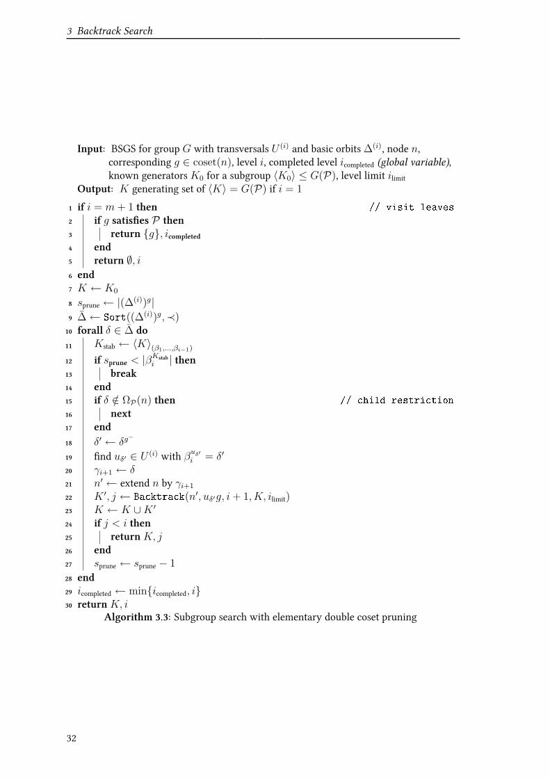
3 Backtrack Search
Input: BSGS for group G with transversals U (i) and basic orbits ∆(i), node n,corresponding g ∈ coset(n), level i, completed level icompleted (global variable),known generators K0 for a subgroup 〈K0〉 ≤ G(P), level limit ilimit
Output: K generating set of 〈K〉 = G(P) if i = 1
if i = m+ 1 then // visit leaves1
if g satisVes P then2
return g, icompleted3
end4
return ∅, i5
end6
K ← K07
sprune ← |(∆(i))g|8
∆← Sort((∆(i))g,≺)9
forall δ ∈ ∆ do10
Kstab ← 〈K〉(β1,...,βi−1)11
if sprune < |βKstabi | then12
break13
end14
if δ /∈ ΩP(n) then // child restriction15
next16
end17
δ′ ← δg−
18
Vnd uδ′ ∈ U (i) with βuδ′i = δ′19
γi+1 ← δ20
n′ ← extend n by γi+121
K ′, j ← Backtrack(n′, uδ′g, i+ 1, K, ilimit)22
K ← K ∪K ′23
if j < i then24
return K, j25
end26
sprune ← sprune − 127
end28
icompleted ← minicompleted, i29
return K, i30
Algorithm 3.3: Subgroup search with elementary double coset pruning
32
3.1 Classical backtracking
Algorithm 3.3 further extends Algorithm 3.2 with this P-dependent pruning and prun-ing based on double coset minimality due to Lemma 3.5. We check for problem-dependentrestrictions on line 15. Lines 8 and 12 contain code for double coset minimality pruning. Asalready mentioned,K is by construction a strong generating set with respect to the baseBof the inputG. Hence we can easily compute the i-th elementKstab := K [i] = K(β1,...,βi−1)
of the subgroup chain ofK . This computation is performed in line 11. Note that we speakof K in this text and formally use 〈K〉 in the algorithm because in the text we mean Kto be whole known subgroup, whereas in the algorithm K is only a set of generators forG(P). With the subgroup Kstab we then compute the i-th basic orbit βKstab
i of K , whoselength we need in our double coset pruning. Finally, sprune is set to the number of elementsin ∆. If this drops below |βK[i]
i | in line 12 we can stop by Lemma 3.5.
In the following we will examine specializations for the set stabilization and groupintersection problem. Both [Ser03, Sec. 9.1.2] and [HEO05, Sec. 4.6] contain problem-speciVc pruning methods for other problems like centralizers and normalizers.
Setwise stabilizer
Given G ≤ Sym(Ω) and a set ∆ ⊆ Ω, we want to Vnd generators of the setwise stabilizerG∆ of ∆. We start with computing a BSGS (B, S) for G in which all elements of ∆precede Ω \ ∆ in the base. Let k be the Vrst index for which βk /∈ ∆. We can alwaysVnd such an index by extending the base with possibly redundant base points from Ω \∆.Then we already have computed a subgroup G[k] = G(β1,...,βk−1) = G(∆) ≤ G∆, namelythe pointwise stabilizer of ∆.
[Ser03, Sec. 9.1.2] also contains the observation that we only have to traverse the searchtree up to level k− 1. Note that for a node n = (γ1, . . . , γk−1) of the search tree we eitherhave coset(n) ⊆ G∆ (in other terms γ1, . . . , γk−1 ⊆ ∆) or coset(n) ∩ G∆ = ∅. Thus,if coset(n) ⊆ G∆ holds, Lemma 3.3 on page 28 tells us that one generator from the cosetis enough. Naturally, in the other case coset(n) ∩G∆ = ∅ we also prune the node.For the nodes at level i < k − 1 we also do not have to consider all children. It is
obviously enough to traverse all children where γi+1 ∈ ∆. So with the notation fromabove,
ΩP(n) ≡ ∆ for i < k − 1. (3.4)
Because we have found a lot of specializations for the set stabilizer problem we summa-rize all changes in a separate algorithm description. Algorithm 3.5 computes the setwisestabilizer G∆ and calls Algorithm 3.4 as Backtrack. Algorithm 3.4 specializes Algorithm3.3 by three features.
First, we limit the length of the base image we consider to ilimit, which is originallycomputed in line 2 of Algorithm 3.5. When in the backtrack search of Algorithm 3.4 thislimit is reached at the check in line 1, we abort the search. In the special case that we arein the Vrst branch of the search tree, corresponding to g being the identity, we add thegenerators of G[i] = G(∆), which is a subgroup of G∆, to our result set K .
Second, we apply the ΩP(n) restriction. The images of the Vrst base points, which areby construction in Algorithm 3.5 a subset of ∆, have to remain in ∆ as described in (3.4).This check is performed in line 20.
33

3 Backtrack Search
Input: BSGS for group G = 〈S〉 with transversals U (i) and basic orbits ∆(i), node n,corresponding g ∈ coset(n), level i, completed level icompleted (global variable),known generators K0 for setwise stabilizer 〈K0〉 ≤ G∆, level limit ilimit
Output: K generating set of 〈K〉 = G∆ if i = 1
if i = ilimit then // visit leaves1
if ∆g = ∆ then2
if g = () then3
K ← S ∩G[i]4
else5
K ← g6
end7
return K, icompleted8
end9
return ∅, i10
end11
K ← K012
sprune ← |(∆(i))g|13
∆← Sort((∆(i))g,≺)14
forall δ ∈ ∆ do15
Kstab ← 〈K〉(β1,...,βi−1)16
if sprune < |βKstabi | then17
break18
end19
if δ /∈ ∆ then // child restriction20
break21
end22
δ′ ← δg−
23
Vnd uδ′ ∈ U (i) with βuδ′i = δ′24
γi+1 ← δ25
n′ ← extend n by γi+126
K ′, j ← Backtrack(n′, uδ′g, i+ 1, K, ilimit)27
K ← K ∪K ′28
if j < i then29
return K, j30
end31
sprune ← sprune − 132
end33
icompleted ← minicompleted, i34
return K, i35
Algorithm 3.4: Set stabilizer search with elementary double coset pruning
34
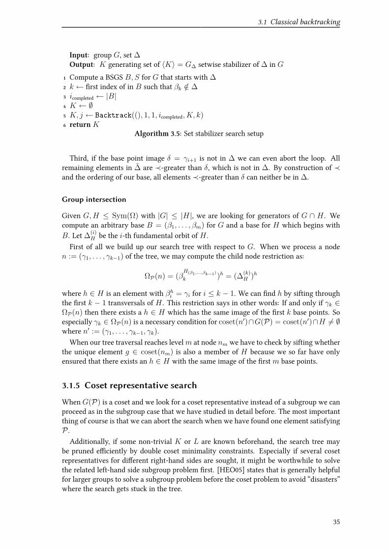
3.1 Classical backtracking
Input: group G, set ∆Output: K generating set of 〈K〉 = G∆ setwise stabilizer of ∆ in G
Compute a BSGS B, S for G that starts with ∆1
k ← Vrst index of in B such that βk /∈ ∆2
icompleted ← |B|3
K ← ∅4
K, j ← Backtrack((), 1, 1, icompleted, K, k)5
return K6
Algorithm 3.5: Set stabilizer search setup
Third, if the base point image δ = γi+1 is not in ∆ we can even abort the loop. Allremaining elements in ∆ are ≺-greater than δ, which is not in ∆. By construction of ≺and the ordering of our base, all elements ≺-greater than δ can neither be in ∆.
Group intersection
Given G,H ≤ Sym(Ω) with |G| ≤ |H|, we are looking for generators of G ∩ H . Wecompute an arbitrary base B = (β1, . . . , βm) for G and a base for H which begins withB. Let ∆
(i)H be the i-th fundamental orbit of H .
First of all we build up our search tree with respect to G. When we process a noden := (γ1, . . . , γk−1) of the tree, we may compute the child node restriction as:
ΩP(n) = (βH(β1,...,βk−1)
k )h = (∆(k)H )h
where h ∈ H is an element with βhi = γi for i ≤ k − 1. We can Vnd h by sifting throughthe Vrst k − 1 transversals of H . This restriction says in other words: If and only if γk ∈ΩP(n) then there exists a h ∈ H which has the same image of the Vrst k base points. Soespecially γk ∈ ΩP(n) is a necessary condition for coset(n′)∩G(P) = coset(n′)∩H 6= ∅where n′ := (γ1, . . . , γk−1, γk).
When our tree traversal reaches levelm at node nm we have to check by sifting whetherthe unique element g ∈ coset(nm) is also a member of H because we so far have onlyensured that there exists an h ∈ H with the same image of the Vrstm base points.
3.1.5 Coset representative search
WhenG(P) is a coset and we look for a coset representative instead of a subgroup we canproceed as in the subgroup case that we have studied in detail before. The most importantthing of course is that we can abort the search when we have found one element satisfyingP .Additionally, if some non-trivial K or L are known beforehand, the search tree may
be pruned eXciently by double coset minimality constraints. Especially if several cosetrepresentatives for diUerent right-hand sides are sought, it might be worthwhile to solvethe related left-hand side subgroup problem Vrst. [HEO05] states that is generally helpfulfor larger groups to solve a subgroup problem before the coset problem to avoid “disasters”where the search gets stuck in the tree.
35

3 Backtrack Search
Applied to the set stabilizer case, where the coset case is by far more importantthan for group intersections, this means the following. Assume that we have sets∆,Γ1,Γ2, . . . ,Γm ⊆ Ω and want to know whether elements g1, . . . , gm ∈ G exist suchthat ∆g1 = Γ1, . . . ,∆
gm = Γm. Then it may be beneVcial to computeG∆ Vrst because wecan use it as K for double coset pruning as clearly ∆g = Γ ⇐⇒ ∆(G∆g) = Γ. Of coursewe also have to adapt the constraint (3.4) and replace it by ΩP(n) ≡ Γ.
3.2 Partition backtracking
The backtracking approach we have seen so far has one big disadvantage: it works onlywith one (base) point at the same time. However, it is often possible to put the knowledgeof all prior decisions to good use and further prune the tree. To illustrate this we take alook at an example from graph theory.
1 2
5 4
36
Figure 3.3: Graph automorphism example
Example 3.6. If we want to compute all automorphism of the graph depicted in Figure3.3, i. e. all permutations that leave the graph structure unchanged, we also can em-ploy backtracking. First we observe that all automorphisms must preserve the triangu-lar structure of 1, 5, 6 and 2, 3, 4. More formally, we have an unordered partitionΠ := 1, 5, 6, 2, 3, 4 of all vertices which every automorphism must not change.Starting our backtrack search at vertex 1, we can choose among 1, 2, 4 and 5, which havethe same valency, for the image of 1. Choosing, for instance, 2 as the image of 1 has im-mediate implications on the possibilities we have for the remaining vertices. Because wehave to preserve Π it follows that 5, 6 has to be mapped onto 3, 4. Due to the degreesof these vertices we then must map 3 onto 6 and 4 onto 5. This gives us one automorphism(1 2)(3 6)(4 5) of the graph. Note that without the knowledge of the conservation of Π wemight have tried to choose 4 as the image of 2 during our backtrack search and only laterfound out that it does not lead to a correct solution.
Backtracking methods based on partitions were introduced by McKay in the 1980s inthe realm of graph automorphisms (cf. [McK81] and the software [nauty]). Later on in1991 Leon successfully applied partition-based backtracking to group theoretical problems(cf. [Leo91, Leo97]), extending his previous work on automorphisms of combinatorial ob-jects such as matrices and linear codes (cf. [Leo84]). Theißen worked separately at the dif-Vcult special case of computing normalizers (cf. [The97]). In this section we concentrate on
36
3.2 Partition backtracking
the application of Leon’s ideas to the set stabilizer and group intersection problem, which– as in the case of the classical backtrack search – are only a sample of problems where thismethod is applicable. The general framework is still abstract enough to allow the searchfor automorphisms of discrete and combinatorial objects such as matrices, graphs or linearcodes (cf. [Leo91]). A patched derivative of Leon’s original partition backtracking imple-mentation, for instance, is still used in the GAP package [GUAVA] for computation withcodes.
3.2.1 Introduction to partitions
First we need to clarify the central term of a partition that has already been introducedinformally in our graph example. It will become clear immediately that we need orderedinstead of unordered partitions to backtrack properly.
DeVnition 3.7. An ordered partition Π = (Π1, . . . ,Πk) of Ω is a sequence of non-empty,pairwise disjoint subsets Πi ⊆ Ω such that
⋃ki=1 Πi = Ω. The sets Πi are called cells of
Π. We denote the length of Π by |Π| := k and the set of all ordered partitions by OP(Ω).The group Sym(Ω) acts cellwise on ordered partitions: Πg := (Πg
1, . . . ,Πgk) for every
g ∈ Sym(Ω).
We prefer ordered partitions to unordered partitions because two ordered partitionsΠ,Σ ∈ OP(Ω) with |Π| = |Σ| = |Ω|, i. e. consisting of only single-element cells, induceexactly one permutation g ∈ Sym(Ω) by Πg = Σ. In the following we refer to orderedpartitions of Ω simply as partitions. An important relation between partitions is that of areVnement:
DeVnition 3.8. Let Π = (Π1, . . . ,Πl) and Σ = (Σ1, . . . ,Σm) be partitions. We say thatΠ is a reVnement of Σ, Π ≤ Σ, if the cells of Σ are a consecutive union of cells ofΠ. Formally, Σi =
⋃kij=ki−1+1 Πj for some indices 0 = k0 < k1 < · · · < km = l. A
reVnement is strict if |Π| > |Σ| and we write Π Σ in this case.
The central concept of our partition backtracking will be a reVnement process that insome way harmonizes with the property P we are looking for.
DeVnition 3.9. A P-reVnementR is a mappingR : OP(Ω)→ OP(Ω) such that• R(Π) ≤ Π for Π ∈ OP(Ω) and,
• if g ∈ G(P) and Π ∈ OP(Ω) it holds that
R(Π)g = R(Πg). (3.5)
In other words, the operation of a P-reVnement and every g ∈ G(P) on partitionscommute. This means, if g is unknown, we can potentially gain information on g becausewe know how it acts on a Vner partition with less degrees of freedom. To actually createreVnements of partitions we can use an intersection of partitions.
DeVnition 3.10. Let Π = (Π1, . . . ,Πl) and Σ = (Σ1, . . . ,Σm) be partitions. We deVnethe intersection Π ∧ Σ as the partition with the non-empty sets Πi ∩ Σj for 1 ≤ i ≤ l,1 ≤ j ≤ m as cells, ordered by the following rule: Πi1 ∩ Σj1 precedes Πi2 ∩ Σj2 if andonly if i1 < i2 or i1 = i2 and j1 < j2.
37
3 Backtrack Search
Lemma 3.11. Let Π,Σ ∈ OP(Ω). The intersection Π∧Σ is a reVnement of Π. The reversestatement does not hold.
Proof. By deVnition of the intersection we have Π ∧ Σ = (Π1 ∩ Σ1,Π1 ∩ Σ2, . . . ,Π1 ∩Σm,Π2 ∩ Σ1,Π2 ∩ Σ2, . . . ), which is a reVnement of Π. The order in which we havedeVned the intersection to work with cells is also the reason why Π∧Σ is not a reVnementof Σ.
Example 3.12. Consider the set Ω = 1, 2, . . . , 7. We write Π := (1 3 5 | 2 4 | 6 7) in shortfor the partition (1, 3, 5, 2, 4, 6, 7). We have that Σ := (1 3 | 5 | 2 4 | 6 | 7) ≤ Π isa strict reVnement of Π. Because the order into which cells are split up is not relevant,Σ′ := (5 | 1 3 | 4 | 2 | 6 7) ≤ Π is another strict reVnement of Π. We can “isolate” elementsα ∈ Ω of a partition by intersecting with Iα := (α |Ω \ α). For example, to isolate 5 inΠ we compute Π ∧ I5 = (5 | 1 3 | 2 4 | 6 7).
Before we step into technical details we have a brief look at the idea of partition back-tracking. Let us assume we have Π,Σ ∈ OP(Ω) such that for some (possibly unknown)g ∈ G(P) the relation Πg = Σ holds. As mentioned before, Πg := (Πg
1, . . . ,Πgk) means
cellwise action of g on the partition. For instance, the trivial partitions Π = Σ = (Ω) arean obvious starting point. The Vner Π and Σ are, i. e. the more cells they have, the moreinformation we get about g ∈ G(P). If both Π and Σ are discrete, that means all cellsconsist of a single element, the permutation g is uniquely determined.The way to get there are P-reVnements. We start with a pair Π, Σ of ordered partitions
such that Πg = Σ for some g ∈ G(P). Then we try to Vnd P-reVnementsR that actuallyyield Vner partitions Π := R(Π) Π and Σ := R(Σ) Σ. For such a reVnement R weobtain Πg = R(Π)g = R(Πg) = Σ by the P-reVnement property (3.5). We can iteratethis process until we cannot Vnd a better, strict reVnement. If the resulting Π and Σ arenot discrete we resort to backtracking as follows: We pick one cell index 1 ≤ j ≤ |Π| with|Πj| ≥ 2 and one α ∈ Πj . Because Πg = Σ and especially Πg
j = Σj the image αg of αhas to be some β ∈ Σj . In a backtracking manner we probe each of this possible imagecandidates β.
DeVnition 3.13. A backtrack reVnement Bα is a function OP(Ω)→ OP(Ω) deVned as
Bα(Π) := Π ∧ (α,Ω \ α).
So for the next iteration we set Π := Bα(Π) and Σ := Bβ(Σ) for some β ∈ Σj ,assuming that there still is a g ∈ G(P) with Πg = Σ (and αg = β). When we eventuallyreach a discrete partition Σ the pair Π,Σ deVnes a unique g ∈ Sym(Ω) by Πg = Σ. Whatis left to us is to check whether also g ∈ G(P).
Example 3.14. For a small example of the idea we consider G = S3 = 〈(1 2), (2 3)〉 andlook for the stabilizerG3 of 3 inG. We start with Π = Σ = (Ω) = (1 2 3). Because everyg ∈ G(P) = G3 must map 3 onto itself a suitable strict P-reVnement R is R := I3
with Iα from Example 3.12. That means we isolate 3 into a single cell. We thus obtainΠ = I3(Π) = (3 | 1 2) and Σ = I3(Σ) = (3 | 1 2). For every g ∈ G(P) holds Πg = Σ.We cannot Vnd another strict P-reVnement so we start backtracking. We have to pick
the cell 1 2 of Π and choose B1 as backtrack reVnement. Hence we have to consider
38
3.2 Partition backtracking
the pairs B1(Π),B1(Σ) and B1(Π),B2(Σ) next. First we continue with Π := B1(Π) =(3 | 1 | 2) and Σ := B1(Σ) = (3 | 1 | 2). Both cells are discrete so we can read g = (),which obviously is in G(P). The second backtrack alternative is Π := B1(Π) = (3 | 1 | 2)and Σ := B2(Σ) = (3 | 2 | 1). We infer g = (1 2), which also is in G(P). We have nomore alternative left and we thus know G(P) is complete with G(P) = (), (1 2).
3.2.2 Search tree
We begin with a deVnition of an R-base that plays a role similar to the BSGS base inclassical backtracking.
DeVnition 3.15. An R-base is a chain of reVned partitions Π(i), Π(i) together with a pairof P- and backtrack reVnementR(i), Bαi such that
Π(i) = Bαi(Π(i−1)) (3.6)
Π(i) = R(i)(Π(i)) (3.7)
holds for 1 ≤ i ≤ m, starting with Π0 := R(0)(Ω) where R(0) is an initial P-reVnement.The chain ends at the Vrst indexm such that Π(m) is discrete.
We can ensure the Vniteness of the chain by a careful choice of αi for (3.6). As long asΠ(i) is not discrete we Vnd a cell of Π(i) that has at least two elements. Isolating one ofthem yields a strict reVnement.
It is very important to note that an R-base depends not only on the group G to searchin, but also on the property P . Searches for diUerent subgroups of the same group G willlead to diUerent R-bases. So it takes the role of both base and child restriction ΩP(n)(cf. page 31) of classical backtracking.
DeVnition 3.16. Let Π ∈ OP(Ω) be a partition that has been created from Ω by a seriesof reVnements. We deVne fix(Π) as the ordered sequence of single-element cells of Π inthe order in which they appeared in the reVnement process.
Example 3.17. To clarify the meaning of fix we look at the following partitions and their“fix” points
Π(0) = (1 2 3 4 5 6 7) fix Π(0) = ∅≥ Π(1) = (1 2 3 | 4 5 6 7) fix Π(1) = ∅≥ Π(2) = (1 | 2 3 | 4 5 6 7) fix Π(2) = (1)
≥ Π(3) = (1 | 3 | 2 | 4 5 6 7) fix Π(3) = (1, 3, 2)
≥ Π(4) = (1 | 3 | 2 | 4 5 | 6 7) fix Π(4) = (1, 3, 2)
≥ Π(5) = (1 | 3 | 2 | 4 | 5 | 6 7) fix Π(5) = (1, 3, 2, 4, 5)
≥ Π(6) = (1 | 3 | 2 | 4 | 5 | 7 | 6) fix Π(6) = (1, 3, 2, 4, 5, 7, 6)
We are now ready to deVne our search tree for partition backtracking.
39
3 Backtrack Search
DeVnition 3.18. Let Π(i), Π(i), R(i), Bαi be an R-base. Our search tree is a tree withpartitions Σ(i) as node labels and the following properties:
• The root at level 0 has the label Σ(0) := Π(0).
• Let i be an intermediate level 0 ≤ i < m. Let b be the cell index of Π(i) whichcontains αi+1. Then the node Σ(i) has the children
Σ(i+1),β := R(i+1)(Bβ(Σ(i))) for every β ∈ Σ(i)b
for which there exists a g ∈ G with (fix Π(i+1))g = fix Σ(i+1),β . Here we use thesuperscript β in Σ(i+1),β only as a referencing index with no further computationalmeaning.
DeVnition 3.18 is a formal description of the general idea we discussed in the last section.We start with a partition Π(0) from our R-base and the root node Σ(0) which by deVnitionfulVll the relationship
(Π(0))g = Σ(0) ∀g ∈ G(P). (3.8)
In the Vrst level child nodes Σ(1) we Vrst split up our search into all possible cases for theimage of α1. Naming Π(1) := Bα1(Π(0)) and Σ(1),β := Bβ(Σ(0)), equation (3.8) impliesthat
(Π(1))g = Σ(1),β ∀g ∈ G(P) ∩ g ∈ G : αg1 = β. (3.9)
We then apply the P-reVnementR(1) and (3.9) implies together with the reVnement prop-erty (3.5) that
(Π(1))g = Σ(1),β ∀g ∈ G(P) ∩ g ∈ G : αg1 = β. (3.10)
Before we continue with the next backtrack round we would like to know if the restrictionαg1 = β leads to an unsatisVable situation and we may thus skip this node. In generalthis is hard to decide and so we settle for weaker criteria: First of all the number of cells|Π(1)| = |Σ(1)| has to be equal. Second, the sizes of corresponding cells |Π(1)
j | = |Σ(1)j |
have to match for 1 ≤ j ≤ |Π(1)|. At last we check whether there exists at least ag ∈ G which maps the single element cells fix Π(1) onto fix Σ(1). We could easily test thisnecessary requirement if we had a BSGS of G that starts with fix Π(1).
Of course we would like to execute these checks on every level to prune the tree early.Because fix Π(m) is known after the setup of the R-base and because fix Π(i) is a preVxof fix Π(i+1), we compute a BSGS for G with base fix Π(m) once at the beginning. UsingAlgorithm 3.6 on this BSGS, we then can perform checks for (fix Π(i))g = fix Σ(i),β onevery level i.
The leaves of the search tree, discrete partitions Σ(m), correspond uniquely to groupelements g which may or may not be a member of G(P). So the search tree may con-tain more than |G(P)| leaves. By construction we only ensure that every g ∈ G(P)corresponds to a leaf of the tree because we build up a chain of necessary conditions formembership by the P-reVnement property (3.5) on page 37.
Lemma 3.19. For every g ∈ G(P) there exists a leaf Σ(m) of the search tree with(Π(m))g = Σ(m).
40
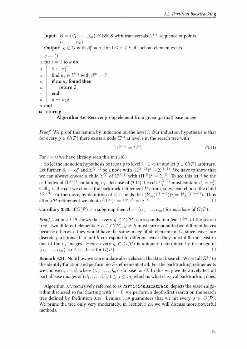
3.2 Partition backtracking
Input: B = (β1, . . . , βm), S BSGS with transversals U (i), sequence of points(α1, . . . , αk)
Output: g ∈ G with βgi = αi for 1 ≤ i ≤ k, if such an element exists
g ← ()1
for i = 1 to k do2
δ ← αg−
i3
Vnd uδ ∈ U (i) with βuδi = δ4
if no uδ found then5
return ∅6
end7
g ← uδg8
end9
return g10
Algorithm 3.6: Recover group element from given (partial) base image
Proof. We proof this lemma by induction on the level i. Our induction hypothesis is thatfor every g ∈ G(P) there exists a node Σ(i) at level i in the search tree with
(Π(i))g = Σ(i). (3.11)
For i = 0 we have already seen this in (3.8).So let the induction hypothesis be true up to level i−1 < m and let g ∈ G(P) arbitrary.
Let further βi := αgi and Σ(i−1) be a node with (Π(i−1))g = Σ(i−1). We have to show thatwe can always choose a child Σ(i) of Σ(i−1) with (Π(i))g = Σ(i). To see this let j be thecell index of Π(i−1) containing αi. Because of (3.11) the cell Σ
(i−1)j must contain βi = αgi .
Cell j is the cell we choose the backtrack reVnement Bβ from, so we can choose the childΣ(i),βi . Furthermore, by deVnition of βi it holds that (Bαi(Π(i−1)))g = Bβi(Σ(i−1)). Thusafter a P-reVnement we obtain (Π(i))g = Σ(i),βi =: Σ(i).
Corollary 3.20. If G(P) is a subgroup then A := (α1, . . . , αm) forms a base of G(P).
Proof. Lemma 3.19 shows that every g ∈ G(P) corresponds to a leaf Σ(m) of the searchtree. Two diUerent elements g, h ∈ G(P), g 6= h must correspond to two diUerent leavesbecause otherwise they would have the same image of all elements of Ω, since leaves arediscrete partitions. If g and h correspond to diUerent leaves they must diUer at least inone of the αi images. Hence every g ∈ G(P) is uniquely determined by its image of(α1, . . . , αm), so A is a base for G(P).
Remark 3.21. Note howwe can emulate also a classical backtrack search. We set allR(i) tothe identity function and perform noP-reVnement at all. For the backtracking reVnementswe choose αi := βi where (β1, . . . , βm) is a base for G. In this way we iteratively test allpartial base images of (β1, . . . , βj), 1 ≤ j ≤ m, which is what classical backtracking does.
Algorithm 3.7, recursively referred to as PartitionBacktrack, depicts the search algo-rithm discussed so far. Starting with i = 0, we perform a depth-Vrst search on the searchtree deVned by DeVnition 3.18. Lemma 3.19 guarantees that we hit every g ∈ G(P).We prune the tree only very moderately, in Section 3.2.4 we will discuss more powerfulmethods.
41
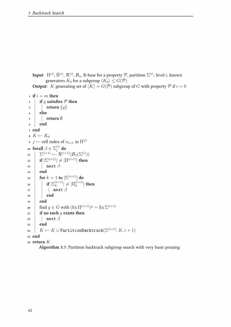
3 Backtrack Search
Input: Π(i), Π(i),R(i), Bαi R-base for a property P , partition Σ(i), level i, knowngenerators K0 for a subgroup 〈K0〉 ≤ G(P)
Output: K generating set of 〈K〉 = G(P) subgroup of G with property P if i = 0
if i = m then1
if g satisVes P then2
return g3
else4
return ∅5
end6
end7
K ← K08
j ← cell index of αi+1 in Π(i)9
forall β ∈ Σ(i)j do10
Σ(i+1) ← R(i+1)(Bβ(Σ(i)))11
if |Σ(i+1)| 6= |Π(i+1)| then12
next β13
end14
for k = 1 to |Σ(i+1)| do15
if |Σ(i+1)k | 6= |Π(i+1)
k | then16
next β17
end18
end19
Vnd g ∈ G with (fix Π(i+1))g = fix Σ(i+1)20
if no such g exists then21
next β22
end23
K ← K ∪ PartitionBacktrack(Σ(i+1), K, i+ 1)24
end25
return K26
Algorithm 3.7: Partition backtrack subgroup search with very basic pruning
42
3.2 Partition backtracking
3.2.3 Constructing an R-base
Now that we know what we need an R-base for we discuss the matter of how to constructone for our problem P . This consists of two independent tasks, which we have to performrepeatedly: Vnding proper P-reVnements and choosing the right αi for the backtrack re-Vnements.
We begin with the choice of the αi. Looking again at the search tree in DeVnition3.18, we see that the size of the backtrack search is bounded by the product d := |Π(0)
j0| ·
|Π(1)j1| · · · · · |Π(m)
jm| where ji denotes the cell index of αi in Π(i). Thus an obvious goal
for the choice of αi is to minimize the product d. A heuristic approach that also is easyto compute is to successively choose ji such that |Π(i)
ji| is minimal. This of course might
not minimize the total product d. Nevertheless, [Leo97, p. 140] states that according to hisexperience this simple heuristic works as good as any other which is easy to implement. Acomputationally more expensive alternative would be to try multiple values of ji for everyi and choose the combination which yields minimal d. We postpone the discussion of thisapproach until the end of this section and turn to a completely diUerent optimization: Aswe will see below, the choice of αi may require a base change to allow for eXcient R-baseconstruction. To reduce the number of base changes, especially proVtable for small groups,we could also try to choose αi so that no base change is required as long as it does notincrease d to much. In an implementation we have to Vnd a compromise between the twoαi-selection strategies. We now turn to the second task in R-base construction, Vndingproper P-reVnements.
For every problemP we can choose from a pool of applicableP-reVnements, dependingon P . To avoid redundancies we are interested in Vnding P-reVnements that yield strictreVnements of the input partition. In the following we examine P-reVnements which wecan try to apply for stabilizing properties or group membership properties.
If P contains the stabilization of a set, we can choose the following:
Lemma 3.22. Let ∆ ⊆ Ω and G(P) ⊆ G∆. Then
Rstab, ∆(Π) := Π ∧ (∆ | Ω \∆) (3.12)
is a P-reVnement.
Proof. Set Σ := (∆ | Ω \ ∆). We have to show that (Πi ∩ Σj)g = Πg
i ∩ Σj for all cellindices i, j and g ∈ G(P). This obviously holds because by deVnition Σ is invariant underaction of G∆ and thus also of G(P), yielding (Πi ∩ Σj)
g = Πgi ∩ Σg
j = Πgi ∩ Σj .
Important to note is that we can apply this P-reVnement for a given ∆ only once toobtain a strict reVnement. The second application of Rstab, ∆ has no more reVnementpower because ∆ and Ω \∆ have already been separated.
Lemma 3.22 is just a reformulation of our observations from Section 3.1.4. The realpower of reVnements for groups lies in exploiting the orbit structures.
DeVnition 3.23. Let G ≤ Sym(Ω). We deVne Θ(G) as the ordered partition of Ω whichconsists of the orbits of Ω under action of G as cells, ordered by the minimal element ofeach orbit.
43
3 Backtrack Search
Example 3.24. Consider G = 〈(1 3)(2 4)(5 6), (1 3)(2 5)(4 6)〉. Then G has the distinctorbits 1G = 1, 3 and 2G = 2, 4, 5, 6. Because min 1G = 1 < 2 = min 2G we obtainΘ(G) = (1 3 | 2 4 5 6).
Lemma 3.25. Let H ≤ Sym(Ω) and G(P) ⊆ H . Let Π ∈ OP(Ω) be given. Then
Rorbit,H , Π(Σ) :=
Σ ∧Θ(Hfix Π)t if there exists a t ∈ H with (fix Π)t = fix Σ
Σ otherwise(3.13)
is a P-reVnement.
Proof. If no such t exists and the second case in (3.13) applies we have nothing to show.So let g ∈ G(P) be arbitrary and Θ := Θ(Hfix Π). We assume there exists a t ∈ H with(fix Π)t = fix Σ. Let u ∈ H with (fix Π)u = fix(Σg). Such a u exists because u = tgwould be a valid choice. To proof the lemmawe have to show that (Σi∩Θt
j)g = Σg
i∩Θuj for
all cell indices i, j and g ∈ G(P). We observe that (fix Π)tgu−
= fix Π, so tgu− ∈ Hfix Π
and thus Θtgu−
j = Θj or in other terms: Θtgj = Θu
j .
A Vrst question when dealing with the P-reVnement of Lemma 3.25 is which partitionΠ to choose. Leon showed in [Leo91, Lemma 8] that, if there is a partition Π that yieldsa strict reVnement Rorbit,H , Π(Σ) of Σ, we can always choose Π := Σ. When we searchfor elements of G(P) and require membership in G it is thus suXcient to check whetherRorbit, G, Π(Π) yields a strict reVnement of our previous partition Π. If we are looking for agroup intersection G ∩H , we can try bothRorbit, G, Π andRorbit,H , Π.
The key for computing Rorbit, G, Π(Π) eXciently in practice is having a base for G thatbegins with fix Π, making generators ofGfix Π available. So whenever fix Π changes duringthe R-base construction we have to change the base of all involved groups such that thesestart again with fix Π.
The two P-reVnements Rorbit and Rstab provide only a sample for the two subgroupproblems we focus on. The interested reader may Vnd in [Leo97, Fig. 2] more P-reVnements for other problems such as centralizers or automorphisms of combinatorialobjects.
As an example Algorithm 3.8 shows the case of R-base construction for a set stabiliza-tion problem. We apply Rstab, ∆ only once at the beginning because multiple applicationsare redundant as discussed above. It remains to try Rorbit, G, Π(i) before resorting to back-tracking. For the backtracking parameters αi we choose the simple strategy of selectinga cell with minimal cardinality. R-base constructions for diUerent problems diUer in thechoice of the considered reVnements. As mentioned above, for G ∩H we would includeRorbit,H , Π(i) parallel toRorbit, G, Π(i) .
Because we compute an R-base only once during the whole partition backtracking pro-cess it may be worthwhile to put more eUort into the R-base construction in order to reducethe search tree size. The parameters we can adjust are: when to apply which reVnementand the choice of the αi. We could even enumerate all or randomly generate and test somereVnement combinations to minimize the search tree size d := |Π(0)
j0| · |Π(1)
j1| · · · · · |Π(m)
jm|.
However, only larger problems might beneVt from such optimizations because the pre-processing eUort gets too large relatively to the problem size.
44

3.2 Partition backtracking
Input: group G ≤ Sym(Ω) and set ∆ ⊆ ΩOutput: R-base for G(P) = G∆
Π(0) ← (Ω)1
R(0) ← Rstab, ∆2
Π(0) ← R(0)(Π(0))3
i← 04
while |Π(i)| 6= |Ω| do5
whileRorbit, G, Π(i)(Π(i)) Π(i) do6
R(i) ← R(i) Rorbit, G, Π(i)7
Π(i) ← Rorbit, G, Π(i)(Π(i))8
change base of G such that it starts with fix Π(i)9
end10
if |Π(i)| 6= |Ω| then11
j ← cell index of Π(i) with minimal cardinality |Π(i)j | ≥ 212
αi ← arbitrary element of Π(i)j13
Π(i+1) ← Bαi(Π(i))14
Π(i+1) ← Π(i+1)15
change base of G such that it starts with fix Π(i+1)16
R(i+1) ← 1 ; // identity refinement17
end18
i← i+ 119
end20
Algorithm 3.8: R-base construction for a set stabilization problem
Still, the value of d is not the only factor determining the time needed for backtracksearch. During the search we may have opportunities to prune the tree, which we cannotforesee in the construction phase. Hence there may be situations in which an R-base thatis not optimal with respect to the product d oUers a better search order for pruning.
3.2.4 Pruning the tree
We can use the same pruning techniques as for classical backtracking in Section 3.1.2,3.1.3 and partly 3.1.4. We can gain the additional advantage from Lemma 3.3 and orderthe child nodes in our search tree. An appropriate order is sorting according to fix Π(m),which contains a base A := (α1, . . . , αm) for G(P) in the subgroup case as we have seenin Corollary 3.20 on page 41. This ordering ensures that we always work at G[i] ∩ G(P)before G \G[i]. Thus we can prune nodes based on Lemma 3.3 and obtain automatically astrong generating set for G(P) relative to the base A.
When we search for a setwise stabilizer G∆ we can apply similar techniques as in Sec-tion 3.1.4 to prune the tree. During the R-base construction we choose the points αi sothat αi lies in ∆, if possible. If for some index k we cannot choose αk ∈ ∆ any longer weVnish the construction as usual until a discrete partition is reached and we thus get a baseA = (α1, . . . , αm) for G∆ which starts with elements from ∆. In the partition backtrack
45
3 Backtrack Search
search we then can abort our search at level k and add G(α1,...,αk−1) ⊆ G∆ to K , like inthe classical backtracking case.
Furthermore, given K ⊆ G(P), it still holds that when we add elements g to the resultsetK in Algorithm 3.7 we can restrict our search to elements minimal in their double coset
KgK . So after the aforementioned ordering we can skip the last s := |αK(α1,...,αi−1)
i | − 1backtracking alternatives due to Lemma 3.5. We may also prune nodes based on Lemma3.4, replacing β1, . . . , βj by α1, . . . αj as subgroup base.
[Leo97, Prop. 6] contains one more necessary condition for double coset minimalitybased on partitions. However, it is more expensive to check and Leon is unsure about itsusefulness.
Input: Π(i), Π(i),R(i), Bαi R-base for a property P , partition Σ(i), level i, completedlevel icompleted (global variable), known generators K0 for a subgroup〈K0〉 ≤ G(P)
Output: K generating set of 〈K〉 = G(P) subgroup of G with property P if i = 0
if i = m then1
if g satisVes P then return g, icompleted;2
else return ∅, i;3
end4
K ← K0;5
j ← cell index of αi+1 in Π(i);6
sprune ← |Σ(i)j |;7
forall β ∈ Sort(Σ(i)j ,≺) do8
Kstab ← 〈K〉(α1,...,αi);9
if sprune < |αKstabi+1 | then break;10
Σ(i+1) ← R(i+1)(Bβ(Σ(i)));11
if |Σ(i+1)| 6= |Π(i+1)| then next β;12
for k = 1 to |Σ(i+1)| do13
if |Σ(i+1)k | 6= |Π(i+1)
k | then14
next β;15
end16
end17
Vnd g ∈ G with (fix Π(i+1))g = fix Σ(i+1);18
if no such g exists then19
next β;20
end21
K ′, l← PartitionBacktrack(Σ(i+1), K, i+ 1);22
K ← K ∪K ′;23
if l < i then return K, l;24
sprune ← sprune − 1;25
end26
icompleted ← minicompleted, i;27
return K, i;28
Algorithm 3.9: Partition backtrack subgroup search with elementary pruning
46

3.2 Partition backtracking
Algorithm 3.9 extends Algorithm 3.7 from page 42 and improves its pruning capabilities.In line 8 we sort the backtracking reVnements according to ≺. We deVne this ordering ≺as α ≺ β for α, β ∈ Ω if and only if α precedes β in fix Π(m), the order in which Vxpoints appear during R-base construction. This ordering allows multi-level backtrackingin line 24 according to Lemma 3.3. Additionally, we can check for double coset minimalityin line 10 due to Lemma 3.5. So this Algorithm 3.9 incorporates the same pruning facilitiesas the classical backtracking Algorithm 3.3 on page 32.
3.2.5 Coset representative search
For partition backtracking the coset case diUers more from the subgroup case than forclassical backtracking. Naturally we can abort the search when we have found one elementsatisfying P . But we also have to extend our search tree formulation and P-reVnementDeVnition 3.9 on page 37.
DeVnition 3.26. A P-reVnement is a pair of mappingsRL,RR : OP(Ω)→ OP(Ω) suchthat
• RL(Π) ≤ Π andRR(Π) ≤ Π for Π ∈ OP(Ω) and,
• if g ∈ G(P) and Π,Σ ∈ OP(Ω) it holds that
Πg = Σ =⇒ RL(Π)g = RR(Σ) (3.14)
This deVnition contains the original one as special case where left and right reVnementRL = RR are equal. In the R-base construction we replace R by RL, in the search treewe useRR instead ofR. The same arguments we used in Section 3.2.2 hold with minimalchanges regarding (3.14) for this case. These show that a partition backtrack search on theextended R-base and search tree Vnds all elements of G(P).
We can extend both Rstab and Rorbit reVnement of Lemma 3.22 and 3.25 according tothe new DeVnition 3.26. However, if we concentrate on the important case of set stabilizercosets we do not have to change Rorbit because the precondition G(P) ⊆ H is still validwhen we look for cosets of H , so we can compute with Rorbit = Rorbit,L = Rorbit,R. WeextendRstab as follows:
Lemma 3.27. Let ∆,Γ ⊆ Ω and ∆g = Γ for all g ∈ G(P). Then
Rstab2, ∆, Γ,L(Π) := Π ∧ (∆ | Ω \∆)
Rstab2, ∆, Γ,R(Σ) := Σ ∧ (Γ | Ω \ Γ)
is a P-reVnement.
Proof. Set Π′ := (∆ | Ω \ ∆) and Σ′ := (Γ | Ω \ Γ). We have to show that for everyg ∈ G(P) the following implication holds:
Πg = Σ ⇒ (Πi ∩ Π′j)g = Σi ∩ Σ′j for all i, j. (3.15)
The condition Πg = Σ implies that Πgi = Σi for all i. Because g ∈ G(P) it holds that
∆g = Γ. Hence we have (Π′j)g = Σ′j and thus (3.15) holds.
47

3 Backtrack Search
Problem P-reVnements to useSetwise stabilizer Rstab,Rorbit Lemma 3.22,3.25Group intersection Rorbit Lemma 3.25Set image Rstab2,Rorbit Lemma 3.27,3.25Coset intersection cf. [Leo97, Fig. 2]
Figure 3.4: Overview of P-reVnements for diUerent problems
The table in Figure 3.4 summarizes the usage of all P-reVnements we examined in thischapter. The interested reader can Vnd in [Leo97, Fig. 2] an extension of Rorbit that canbe used in the coset case of group intersection, which is coset intersection. In this Vgureby Leon there are also P-reVnements described for various other problems such as matrixand group isomorphism.
48
4 Implementation
In this section we will take a closer look at implementation details and the author’s im-plementation PermLib. The author has developed PermLib with three design goals inmind: performance, maintainability and ease of use. The only software dependency is therenowned Boost [Boost] C++ library. It is mostly used for smart pointers, which help toavoid memory leaks. Moreover, unit tests for low-level data structures are provided withinthe Boost test library to control the number of fundamental implementation Waws. Moreinformation about PermLib can be found in Appendix A.In this chapter we Vrst look at data structures for fundamental objects, which we have
not discussed yet. Permutations are core elements of all algorithms, the same is true forpartitions in partition-based backtracking. Because the performance of all other algorithmsthus heavily depends on these basics we have to Vnd data structures that allow us toperform all necessary operations fast and eXciently.After a quick overview of the implementation we look at a series of experiments with
PermLib. It will soon become clear that exhaustive tests go beyond the scope of this thesis,so we just scratch the surface of an extensive survey on computational group theory. Infact we use the experiments to gain some additional insights into the zoo of data structureswe have explored so far. Furthermore, we compare the performance of PermLibwith theother public available state-of-the-art code of GAP and partly Magma. The former is atthe disadvantage of being interpreted at runtime, so that a comparison of actual algorithmimplementations beyond running time is diXcult. The latter is not open source and wasavailable only a special workstation to the author, so not for all experiments Magma resultsare available.
4.1 Low-level data structures
4.1.1 Permutation
Permutations are a central element for all algorithms we have discussed so far, so datastructures for permutations play a key role for fast implementations. A trivial approachis to store a permutation g ∈ Sym(Ω), |Ω| =: n, as an n-dimensional array whose α-th cell contains the image αg. In this way we have access to the image of an element αunder action of g in O(1) time and we can compute the inverse g− in Ω(n) time. How-ever, multiplying two permutations takes Ω(n2) time. We call this form of permutationimplementation elementary permutations.A more sophisticated approach are so called permutation words, as for example de-
scribed in [HEO05, Sec. 4.4.3]. The idea is to store g as a list (or word) of other permu-tations (s1s2 . . . sl), representing the product s1s2 · · · sl. When we choose the si from aVxed “representative” label set S ≤ Sym(Ω), which we store as elementary permutations,
49
4 Implementation
it is enough to store g = s1s2 · · · sl as pointers to elements si. Storing all permutationsin double-linked lists allows multiplication in constant time O(1) by list concatenation.Computing the image αg = αs1s2···sl , however, takes Ω(l) time. If we store for every s ∈ Salso s− ∈ S then we can invert g by reversing the list and replacing each pointer si by s−i ,also summing up to Ω(l) time.
A canonical choice for the label set S is a strong generating set for a group G withrespect to a certain base that we are interested in, adjoined by generator inverses. Duringcomputations, e. g. a base change, new generators may arise, Vrst as words in the originalgenerators. We can multiply them out completely and add them to the label set togetherwith their inverse as elementary permutations.
Choosing between storing permutations completely as image arrays and as permutationwords is a trade-oU between speed of image access and multiplication. With increasing nan Ω(n2) eUort for frequently occurring multiplications becomes more and more infeasi-ble. On the other hand, we often require only a fraction of all possible images so that thepenalty for using words gets not too big.
Because permutations are such a fundamental instrument for our computations, thespeed depends very much on the quality and techniques of permutation implementa-tions. For PermLib both elementary permutations and permutation words have been im-plemented and their usage can be exchanged almost transparently. A very important issuefor permutation words is when words should be multiplied out. This is hard to decideautomatically so it can and should be triggered by the user if necessary. At the momentPermLib multiplies words out only if they are used as group generators.
The current permutation word implementation also is unable to automatically cleargenerators that are no longer used in any word from its storage. Although some kind ofsmart pointer would seem suitable for this purpose, the author has not succeeded yet witha comparably fast implementation based on a smart pointer without losing the ability offast permutation inversion. Nevertheless, an automatic resource deallocation could alsobe implemented for the current version by manual reference counting.
4.1.2 Partition
Leon referenced both in [Leo91, Leo97] an additional paper that was yet to come anddealt with implementation techniques for partition backtracking. However, this paper hasnever appeared, but in [Leo97, p. 130] one can Vnd a sketch of a data structure Leon pro-posed for partitions. A quick analysis of the GAP source code reveals that GAP uses verysimilar structures. The data structures for partitions are a crucial element for a partitionbacktracking implementation to become fast so we take a look at current public state-of-the-art. Closed source-implementations like [Magma] may still do it diUerently.
An obvious requirement for a partition data structure in the context of backtrackingis the ability to perform fast intersections. A less obvious requirement that the authorexperienced during his experiments also is fast intersection reverting, i. e. recovering theoriginal partition Π from Π′ := Π ∧ Σ. This is because copying complete partitions inmemory with their O(n) size as it would be necessary when diving into recursion is tooexpensive to yield competitive performance. Leon’s approach for recovery mitigates thiseUect.
50

4.1 Low-level data structures
Leon proposes the use of seven arrays to represent a partition but a lower number isalready suXcient. In the following we use four arrays to represent a partition Π ∈ OP(Ω),where OP(Ω) denotes the set of all ordered partitions of Ω. We set n := |Ω| and k := |Π|.• partition[1..n] is an ordering of the numbers 1 to nwhere elements of the samecell are stored contiguously and that is consistent with the following three arrays.
• cellSize[1..k] contains at position i the size |Πi| of the i-th cell of Π.
• cellStart[1..k] contains at position i the index of the the Vrst el-ement of cell Πi in partition. This means the i-th cell Πi con-sists of partition[cellStart[i]], partition[cellStart[i] + 1], . . . ,partition[cellStart[i] + cellSize[i] - 1].
• cellOf[1..n] contains at position i the cell number c such that i ∈ Πc.The array cellOf is not necessary to deVne a partition and is used only to enhance perfor-mance of recovering. Before we go into the details of recovery we start with intersection.The intersection operation as deVned in DeVnition 3.10 on page 37 is a convenient way
to describe mathematically a reVnement process but is not usable in an implementation.Usually only a small part of the |Π| · |Σ| intersections in Π ∧ Σ have a non-trivial result.For instance, we can always skip all single-element cells of Π. Hence it is better from analgorithmic point of view to deVne an operation intersect : OP(Ω)→ OP(Ω) as
intersect(Π, i,Γ) :=
(Π1, . . . ,Πi−1,Πi ∩ Γ,Πi \ Γ,Πi+1, . . . ,Πm) if ∅ ( Πi ∩ Γ ( Πi
Π otherwise(4.1)
the intersection of the i-th cell of Π with a set Γ ⊆ Ω. We then can write Π∧Σ as a seriesof consecutive intersections for some indices (i1, j1), . . . , (il, jl):
Π ∧ Σ := intersect(. . . (intersect(intersect(Π, i1,Σj1), i2,Σj2), . . . , il,Σjl) (4.2)
Note that the i1, i2, . . . , il need not to be pairwise diUerent when we have to intersect onecell Σs with diUerent cells of Π. Back to our data structure, this means that for intersect wehave to split up a cell of Π. To facilitate this operation we maintain that every contiguoussegment of partition[] that corresponds to a cell of Π is sorted. Additionally, we requirethat the intersecting set Γ is also a sorted list. Under these conditions we can compute bothΠi ∩ Γ and Πi \ Γ fast in O(|Γ|+ |Πi|) time (cf. [Knu98, Sec. 5.3.2]).In partition[] we split the area corresponding to cell i into two cells by introducing
a new cell index m := |Π| + 1, adjusting cellStart, cellSize and cellOf of i and mand moving elements in the partition area as required by the cell split. In doing so, wemaintain that both emerging cells are still sorted. After Π′ := intersect(Π, i,Γ) we thushave cells Π′i = Πi∩Γ, Π′m = Πi \Γ and Π′j = Πj for all other cells j. If we establish thatΠ = intersect(Π, i,Γ), we do not have to change anything. Technically, the reVnementrelation intersect(Π, i,Γ) ≤ Π does not necessarily hold because the cell indices i,mneed not to be adjacent as required by DeVnition 3.8 on page 37. But this is only a labelingissue, which we can omit in an implementation for eXciency reasons without violatingtheoretical properties established before. Figure 4.1 depicts an example of relevant parts ofa partition data structure before and after an intersection.Our second requirement for the partition data structure is recovering. If we have the
result Π′ := intersect(Π, i,Γ) of a intersection and Π′ Π we can recover Π in the
51
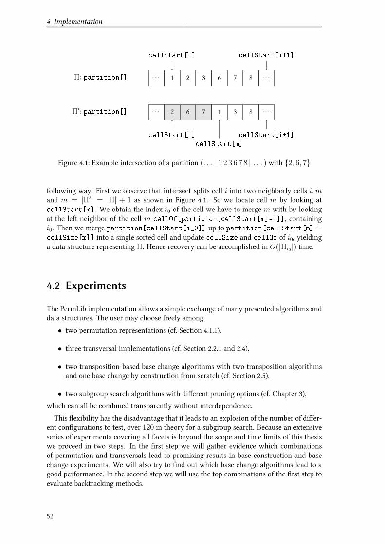
4 Implementation
. . . 1 2 3 6 7 8 . . .
. . . 2 6 7 1 3 8 . . .
cellStart[i] cellStart[i+1]
cellStart[i]
cellStart[m]
cellStart[i+1]
Π: partition[]
Π′: partition[]
Figure 4.1: Example intersection of a partition (. . . | 1 2 3 6 7 8 | . . . ) with 2, 6, 7
following way. First we observe that intersect splits cell i into two neighborly cells i,mand m = |Π′| = |Π| + 1 as shown in Figure 4.1. So we locate cell m by looking atcellStart[m]. We obtain the index i0 of the cell we have to merge m with by lookingat the left neighbor of the cell m cellOf[partition[cellStart[m]-1]], containingi0. Then we merge partition[cellStart[i_0]] up to partition[cellStart[m] +
cellSize[m]] into a single sorted cell and update cellSize and cellOf of i0, yieldinga data structure representing Π. Hence recovery can be accomplished in O(|Πi0|) time.
4.2 Experiments
The PermLib implementation allows a simple exchange of many presented algorithms anddata structures. The user may choose freely among
• two permutation representations (cf. Section 4.1.1),
• three transversal implementations (cf. Section 2.2.1 and 2.4),
• two transposition-based base change algorithms with two transposition algorithmsand one base change by construction from scratch (cf. Section 2.5),
• two subgroup search algorithms with diUerent pruning options (cf. Chapter 3),
which can all be combined transparently without interdependence.
This Wexibility has the disadvantage that it leads to an explosion of the number of diUer-ent conVgurations to test, over 120 in theory for a subgroup search. Because an extensiveseries of experiments covering all facets is beyond the scope and time limits of this thesiswe proceed in two steps. In the Vrst step we will gather evidence which combinationsof permutation and transversals lead to promising results in base construction and basechange experiments. We will also try to Vnd out which base change algorithms lead to agood performance. In the second step we will use the top combinations of the Vrst step toevaluate backtracking methods.
52
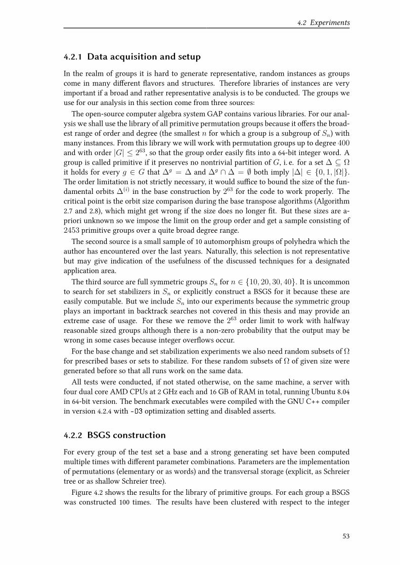
4.2 Experiments
4.2.1 Data acquisition and setup
In the realm of groups it is hard to generate representative, random instances as groupscome in many diUerent Wavors and structures. Therefore libraries of instances are veryimportant if a broad and rather representative analysis is to be conducted. The groups weuse for our analysis in this section come from three sources:The open-source computer algebra system GAP contains various libraries. For our anal-
ysis we shall use the library of all primitive permutation groups because it oUers the broad-est range of order and degree (the smallest n for which a group is a subgroup of Sn) withmany instances. From this library we will work with permutation groups up to degree 400and with order |G| ≤ 263, so that the group order easily Vts into a 64-bit integer word. Agroup is called primitive if it preserves no nontrivial partition of G, i. e. for a set ∆ ⊆ Ωit holds for every g ∈ G that ∆g = ∆ and ∆g ∩ ∆ = ∅ both imply |∆| ∈ 0, 1, |Ω|.The order limitation is not strictly necessary, it would suXce to bound the size of the fun-damental orbits ∆(i) in the base construction by 263 for the code to work properly. Thecritical point is the orbit size comparison during the base transpose algorithms (Algorithm2.7 and 2.8), which might get wrong if the size does no longer Vt. But these sizes are a-priori unknown so we impose the limit on the group order and get a sample consisting of2453 primitive groups over a quite broad degree range.The second source is a small sample of 10 automorphism groups of polyhedra which the
author has encountered over the last years. Naturally, this selection is not representativebut may give indication of the usefulness of the discussed techniques for a designatedapplication area.The third source are full symmetric groups Sn for n ∈ 10, 20, 30, 40. It is uncommon
to search for set stabilizers in Sn or explicitly construct a BSGS for it because these areeasily computable. But we include Sn into our experiments because the symmetric groupplays an important in backtrack searches not covered in this thesis and may provide anextreme case of usage. For these we remove the 263 order limit to work with halfwayreasonable sized groups although there is a non-zero probability that the output may bewrong in some cases because integer overWows occur.For the base change and set stabilization experiments we also need random subsets of Ω
for prescribed bases or sets to stabilize. For these random subsets of Ω of given size weregenerated before so that all runs work on the same data.All tests were conducted, if not stated otherwise, on the same machine, a server with
four dual core AMD CPUs at 2 GHz each and 16 GB of RAM in total, running Ubuntu 8.04in 64-bit version. The benchmark executables were compiled with the GNU C++ compilerin version 4.2.4 with -O3 optimization setting and disabled asserts.
4.2.2 BSGS construction
For every group of the test set a base and a strong generating set have been computedmultiple times with diUerent parameter combinations. Parameters are the implementationof permutations (elementary or as words) and the transversal storage (explicit, as Schreiertree or as shallow Schreier tree).Figure 4.2 shows the results for the library of primitive groups. For each group a BSGS
was constructed 100 times. The results have been clustered with respect to the integer
53
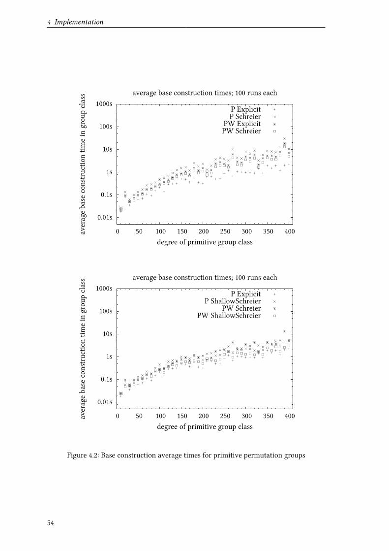
4 Implementation
0.01s
0.1s
1s
10s
100s
1000s
0 50 100 150 200 250 300 350 400averagebase
constructio
ntim
ein
grou
pclass
degree of primitive group class
average base construction times; 100 runs each
P ExplicitP Schreier
PW ExplicitPW Schreier
0.01s
0.1s
1s
10s
100s
1000s
0 50 100 150 200 250 300 350 400averagebase
constructio
ntim
ein
grou
pclass
degree of primitive group class
average base construction times; 100 runs each
P ExplicitP ShallowSchreier
PW SchreierPW ShallowSchreier
Figure 4.2: Base construction average times for primitive permutation groups
54
4.2 Experiments
tenth of the degree, so degrees 10 to 19, 20 to 29, 30 to 39 &c. each form a class in thechart. Because the running time of the Schreier-Sims algorithm depends on both degreeand order, this clustering regardless of the group structure is quite arbitrary and onlyused to Vnd a presentable form. Throughout this chapter P and PW in a legend standfor elementary permutation implementation and implementation as permutation word,respectively. The second term in the legend speciVes the used transversal implementation.For almost all classes explicit transversals together with an elementary permutation im-
plementation are the fastest combination. Elementary permutations used together with aSchreier tree transversal are throughout the sample the slowest combination. Permutationwords work better with Schreier tree transversals but are still outperformed by elementarypermutations and explicit transversals.That explicit and Schreier tree transversals show very similar performance when used
with permutation words is not by accident. Because permutations words in explicittransversals are usually not multiplied out but words in generators, “explicit” transver-sals for permutation words are just another form of Schreier tree storage and not reallyexplicit. In this implementations the performance variation is caused by memory opera-tion patterns which in this case favor explicit transversals slightly.The reason why Schreier tree transversal implementations both with elementary per-
mutations and permutation words are slowest has two diUerent reasons. Because theSchreier-Sims construction mainly consists of building Schreier generators a lot of multi-plications are needed to build the transversal elements from the tree. This high numberof multiplications is the reason why the combination “P Schreier” is slow. We could al-ready expect this from the asymptotic analysis of the Schreier-Sims algorithm on page 14.Permutations word, on the other hand, are less aUected by the multiplications becausefor these word multiplications are relatively cheap. However, the words still have to bemultiplied out to check if a Schreier generator is the identity. This occurs during theSchreier-Sims construction too often to actually gain a beneVt.It remains to analyze the performance of the shallow Schreier tree variant of Section 2.4
in the bottom part of Figure 4.2. For the primitive groups the shallow Schreier tree im-plementation using permutation words comes very close to the “P Explicit” optimum, andalways at least as fast as the normal Schreier tree variant. The shallow trees together withelementary permutations gain over the normal Schreier trees (not in this Vgure), but arestill inferior to the permutation words with the same transversal technique. These resultsare in accordance with our observations from above that the major factor of Schreier treeperformance is the multiplications to construct a transversal element. Shallow Schreiertrees reduce this number of edge label multiplications and are thus faster.Figure 4.3 shows results for the Schreier-Sims algorithm implementation on the sym-
metric groups Sn for n ∈ 10, 20, 30, 40. The algorithm conVgurations which the pre-liminary evidence of the primitive group library lets us suppose to be slow are omit-ted. Only the three most promising variants are shown and compared with GAP. TheGAP calls used were as close to the API of the C++ implementation as possible, call-ing StabChain(Group(...)) on a list of generators. The running times of PermLib arerather indiUerent, with increasing degree the Shallow tree variant with permutation wordshas a minimal lead over the rest. At least for these examples the C++ implementation cancompete with GAP performance. For this special case Sn, however, there are faster ways toconstruct a BSGS in GAP by calling SymmetricGroup(n) directly instead of Group(.).
55

4 Implementation
0.1s
1s
10s
100s
1000s
10000s
S10 S20 S30 S40
base
constructio
ntim
e
symmetric group
base construction times; 1000 runs each
P ExplicitPW Schreier
PW ShallowSchreierGAP 4.4.10
Figure 4.3: Base construction times for symmetric groups
0.01s
0.1s
1s
10s
100s
1000s
E6
met
5
psmet
5
E7
met
6
psmet
6
bh105
E8
met
7
psmet
7
base
constructio
ntim
e
polyhedron
base construction times; 1000 runs each
P ExplicitPW Schreier
PW ShallowSchreierGAP 4.4.10
Figure 4.4: Base construction times for polyhedral automorphism groups
56
4.2 Experiments
Using this specialization, GAP becomes even faster than the C++ implementation. How-ever, this is no surprise because the set (1 2), (2 3), . . . , (n− 1n) is a strong generatingset relative to any n − 1 points from Ω. Hence there is nothing really to compute and itonly remains to set up the transversal data structures.Finally, we look at the test set coming from practice, the polyhedral automorphism
groups. Figure 4.4 shows the results of the runs with the top three performance parametercombinations and GAP. The automorphism groups are ordered by degree ascendingly fromleft (E6 with degree 36) to right (psmet7 with degree 154). From the PermLibvariations noone dominates the other. Rather a correlation between winning parameter combinationand polyhedron class (Ex, metx, psmetx) can be suspected. The result pattern of GAPsuggests there is a certain minimal time for initialization. At least this would explain whyGAP comes closer to the C++ implementation for bigger instances than for the smallerones.
4.2.3 Base change
Besides the two parameters from the last section, permutation and transversal implemen-tation, we have two additional degrees of freedom for base change algorithms: the basechange algorithm• “simple”, Algorithm 2.6 with transpositions only,
• “conjugation”, Algorithm 2.9 with transposition and conjugation,
• “construction”, Algorithm 2.10 re-construction from scratch,and the base transposition algorithm for the transposition-based change algorithms.To gather quickly evidence which combination works best with which permutation and
transversal implementation we begin with experiments on a subset of the primitive grouplibrary. Instead of testing each of the 2453 groups from the library with a small number ofbase changes we perform many base changes on a smaller subset. We will use all primitivegroups of degree 50, 100, 400 and a random selection of primitive groups of degree 256,which still gives us 109 groups to work with. Because we have to randomly generateprescribed bases for every degree that we want to test, this selection of four diUerentdegrees also helps to bound the experiment eUorts. The numbers 50, 100, 256 and 400themselves are not important, it is meant to be a not too small selection of groups withincreasing degree.First we examine the base transposition algorithms. Therefore we pick the base change
algorithm 2.6 which uses only transpositions so that it is a good indicator for transpositionperformance. For the subset of primitive groups we plug in both the deterministic andthe randomized transposition algorithm and repeatedly change bases according to a pre-computed, randomly generated sequence of base points. Each of these 1000 prescribedbases has length log2 n for a group of degree n, regardless of the actual group order.Figure 4.5 shows the results of deterministic and randomized base point transposition
side by side for four diUerent permutation/transversal implementations. For both elemen-tary permutation variations, the left four columns of each cluster in the Vgure, we see thatthe randomized version is measurably faster than the deterministic version. For the twopermutation words combinations, the four columns on the right, there is only a small dif-ference in the result between deterministic and randomized transposition. Analysis with
57

4 Implementation
0.1s
1s
10s
50 100 256 400
averagebase
change
time
degree of primitive group class
average base change times; 1000 runs each
P Explicit DetP Explicit RandP Schreier Det
P Schreier Rand
PW Schreier DetPW Schreier RandPW Shallow Det
PW Shallow Rand
Figure 4.5: Base change/transposition average times for selected primitive groups
the performance analysis tool Valgrind [Vgrind] and internal statistics suggest that gener-ating random Schreier generators based on permutation words is too slow to beneVt fromthe reduced total generator number. For the remaining experiments we therefore use thedeterministic base transpose algorithm for permutation words and the randomized versionfor elementary permutations.
The next step is to measure running times of the three base change algorithm. Firstwe start with a similar setup: for each primitive group we change the base 1000 timesaccording to a randomly generated list of bases of length blog2 nc. Figure 4.6 shows theresults.
By comparing the left-most and right-most column of each cluster in the Vgure, we seethat the “simple” base change with only transpositions performs always worse than its im-proved variant with conjugation. For most cases base change by construction, representedby the column in the middle, is the fastest method. This is not very surprising as we are infact performing 1000 base constructions per group because the bases are totally unrelated.A more realistic test case would consist of sets that are more similar to each other andshare the same preVx. This allows a better reuse of the previous BSGS elements.
Figure 4.7 shows the results of such a run with 1000 random bases of length 2blog2 ncthat were each generated from their predecessor. Both transposition based algorithms runin almost zero time, whereas the construction method takes a lot of time. The absolutevalues of Figure 4.6 and 4.7 are not comparable because the prescribed base length diUerand in the former run each base change was performed on a copy of a original BSGS and
58
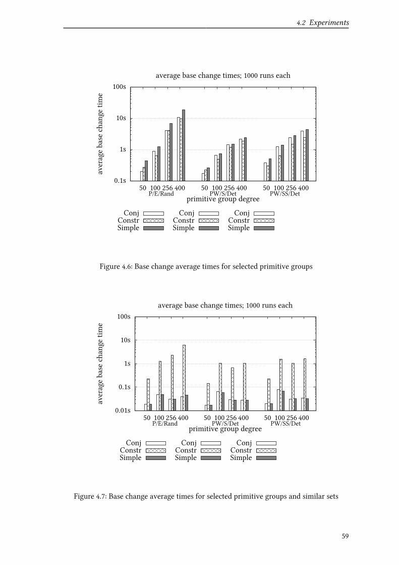
4.2 Experiments
0.1s
1s
10s
100s
50 100 256 400 50 100 256 400 50 100 256 400
averagebase
change
time
primitive group degree
average base change times; 1000 runs each
ConjConstrSimple
ConjConstrSimple
ConjConstrSimple
PW/SS/DetPW/S/DetP/E/Rand
Figure 4.6: Base change average times for selected primitive groups
0.01s
0.1s
1s
10s
100s
50 100 256 400 50 100 256 400 50 100 256 400
averagebase
change
time
primitive group degree
average base change times; 1000 runs each
ConjConstrSimple
ConjConstrSimple
ConjConstrSimple
PW/SS/DetPW/S/DetP/E/Rand
Figure 4.7: Base change average times for selected primitive groups and similar sets
59
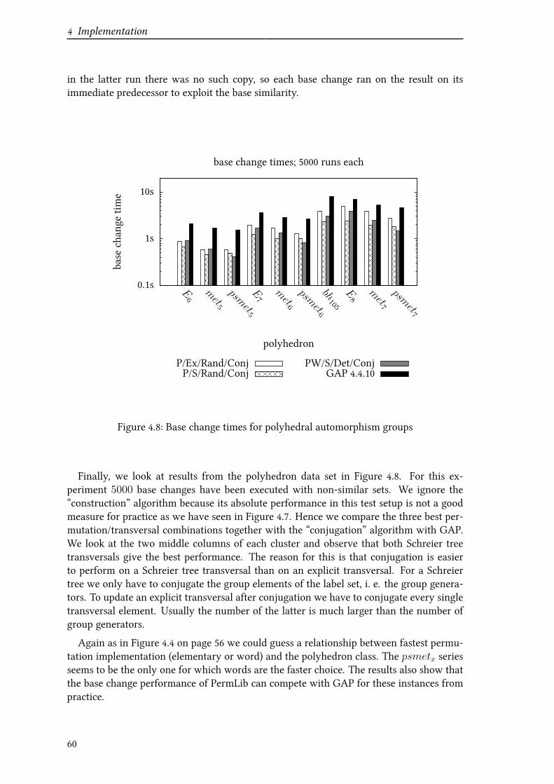
4 Implementation
in the latter run there was no such copy, so each base change ran on the result on itsimmediate predecessor to exploit the base similarity.
0.1s
1s
10s
E6
met
5
psmet
5
E7
met
6
psmet
6
bh105
E8
met
7
psmet
7
base
change
time
polyhedron
base change times; 5000 runs each
P/Ex/Rand/ConjP/S/Rand/Conj
PW/S/Det/ConjGAP 4.4.10
Figure 4.8: Base change times for polyhedral automorphism groups
Finally, we look at results from the polyhedron data set in Figure 4.8. For this ex-periment 5000 base changes have been executed with non-similar sets. We ignore the“construction” algorithm because its absolute performance in this test setup is not a goodmeasure for practice as we have seen in Figure 4.7. Hence we compare the three best per-mutation/transversal combinations together with the “conjugation” algorithm with GAP.We look at the two middle columns of each cluster and observe that both Schreier treetransversals give the best performance. The reason for this is that conjugation is easierto perform on a Schreier tree transversal than on an explicit transversal. For a Schreiertree we only have to conjugate the group elements of the label set, i. e. the group genera-tors. To update an explicit transversal after conjugation we have to conjugate every singletransversal element. Usually the number of the latter is much larger than the number ofgroup generators.
Again as in Figure 4.4 on page 56 we could guess a relationship between fastest permu-tation implementation (elementary or word) and the polyhedron class. The psmetx seriesseems to be the only one for which words are the faster choice. The results also show thatthe base change performance of PermLib can compete with GAP for these instances frompractice.
60
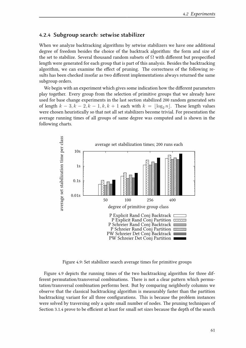
4.2 Experiments
4.2.4 Subgroup search: setwise stabilizer
When we analyze backtracking algorithms by setwise stabilizers we have one additionaldegree of freedom besides the choice of the backtrack algorithm: the form and size ofthe set to stabilize. Several thousand random subsets of Ω with diUerent but prespeciVedlength were generated for each group that is part of this analysis. Besides the backtrackingalgorithm, we can examine the eUect of pruning. The correctness of the following re-sults has been checked insofar as two diUerent implementations always returned the samesubgroup orders.We begin with an experiment which gives some indication how the diUerent parameters
play together. Every group from the selection of primitive groups that we already haveused for base change experiments in the last section stabilized 200 random generated setsof length k − 3, k − 2, k − 1, k, k + 1 each with k = blog2 nc. These length valueswere chosen heuristically so that not all set stabilizers become trivial. For presentation theaverage running times of all groups of same degree was computed and is shown in thefollowing charts.
0.01s
0.1s
1s
10s
50 100 256 400
averagesetstabilizationtim
eperclass
degree of primitive group class
average set stabilization times; 200 runs each
P Explicit Rand Conj BacktrackP Explicit Rand Conj Partition
P Schreier Rand Conj BacktrackP Schreier Rand Conj Partition
PW Schreier Det Conj BacktrackPW Schreier Det Conj Partition
Figure 4.9: Set stabilizer search average times for primitive groups
Figure 4.9 depicts the running times of the two backtracking algorithm for three dif-ferent permutation/transversal combinations. There is not a clear pattern which permu-tation/transversal combination performs best. But by comparing neighborly columns weobserve that the classical backtracking algorithm is measurably faster than the partitionbacktracking variant for all three conVgurations. This is because the problem instanceswere solved by traversing only a quite small number of nodes. The pruning techniques ofSection 3.1.4 prove to be eXcient at least for small set sizes because the depth of the search
61

4 Implementation
tree is bounded by |∆| and only nodes with γi ∈ ∆ have to be considered. For larger setswe observe a diUerent situation, though.
Figure 4.10 shows the results of a single groupG of degree 100 and order about 1.2·1012.For this run sets ∆ of size 2 to 25 were randomly generated. For 50 sets of each size thestabilizer G∆ was computed, for |∆| ≥ 13 the group G∆ had always order 2 or less. Asshown for the small sets, classical backtracking beats partition backtracking because it hasno overhead with partition handling for the small number of nodes. With increasing setsize and also traversed node number the partition backtracking implementation becomesmore and more eXcient.
0.1s
1s
10s
100s
5 10 15 20 25
setstabilizationtim
e
size of sets
set stabilization times for 50 runs each
P Explicit Rand Conj BacktrackP Explicit Rand Conj Partition
Figure 4.10: Set stabilizer search time depending on set size
In the next experiment we examine the inWuence of double coset minimality accordingto Lemma 3.4 on page 30. This is the only double coset minimality criterion we looked atthat has signiVcant costs because it possibly involves base changes. So all other presentedcriteria were enabled by default and we just toggle pruning based on Lemma 3.4, whichwe abbreviate with DCM. Figure 4.11 is a continuation of Figure 4.9 on page 61. We cansee that DCM pruning has not a big, measurable eUect on the running times. It tends tomake the search slightly slower because of the additional base changes that are required.This, and the superior performance of classical backtracking for smaller set sizes, are anindication that the number of nodes is already quite near a minimum for backtrack search.
Finally, we compare PermLib with other implementations. We cannot compare withLeon’s original code because it is not well-suited for sequential runs and sometimes caughtsegmentation faults during preliminary experiments. However, we can run experimentswith the computer algebra software Magma [Magma], which states on its homepage that
62
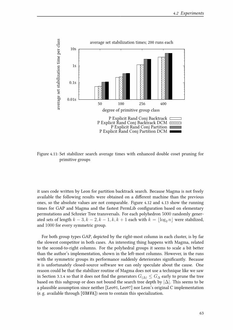
4.2 Experiments
0.01s
0.1s
1s
10s
50 100 256 400
averagesetstabilizationtim
eperclass
degree of primitive group class
average set stabilization times; 200 runs each
P Explicit Rand Conj BacktrackP Explicit Rand Conj Backtrack DCM
P Explicit Rand Conj PartitionP Explicit Rand Conj Partition DCM
Figure 4.11: Set stabilizer search average times with enhanced double coset pruning forprimitive groups
it uses code written by Leon for partition backtrack search. Because Magma is not freelyavailable the following results were obtained on a diUerent machine than the previousones, so the absolute values are not comparable. Figure 4.12 and 4.13 show the runningtimes for GAP and Magma and the fastest PermLib conVguration based on elementarypermutations and Schreier Tree transversals. For each polyhedron 5000 randomly gener-ated sets of length k − 3, k − 2, k − 1, k, k + 1 each with k = blog2 nc were stabilized,and 1000 for every symmetric group.
For both group types GAP, depicted by the right-most column in each cluster, is by farthe slowest competitor in both cases. An interesting thing happens with Magma, relatedto the second-to-right columns. For the polyhedral groups it seems to scale a bit betterthan the author’s implementation, shown in the left-most columns. However, in the runswith the symmetric groups its performance suddenly deteriorates signiVcantly. Becauseit is unfortunately closed-source software we can only speculate about the cause. Onereason could be that the stabilizer routine of Magma does not use a technique like we sawin Section 3.1.4 so that it does not Vnd the generators G(∆) ≤ G∆ early to prune the treebased on this subgroup or does not bound the search tree depth by |∆|. This seems to bea plausible assumption since neither [Leo91, Leo97] nor Leon’s original C implementation(e. g. available through [GUAVA]) seem to contain this specialization.
63

4 Implementation
0.1s
1s
10s
100s
E6
met
5
psmet
5
E7
met
6
psmet
6
bh105
E8
met
7
psmet
7
setstabilizationtim
e
polyhedron
set stabilization times for 5000 runs each
P Schreier Rand Conj BacktrackP Schreier Rand Conj Partition
Magma 2.15GAP 4.4.9
Figure 4.12: Set stabilizer search times for polyhedral automorphism groups
0.1s
1s
10s
100s
1000s
S10 S20 S30 S40
setstabilizationtim
e
symmetric group
set stabilization times for 1000 runs each
P Schreier Rand Conj BacktrackP Schreier Rand Conj Partition
Magma 2.15GAP 4.4.9
Figure 4.13: Set stabilizer search times for symmetric groups
64
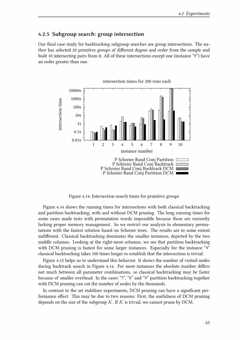
4.2 Experiments
4.2.5 Subgroup search: group intersection
Our Vnal case study for backtracking subgroup searches are group intersections. The au-thor has selected 20 primitive groups of diUerent degree and order from the sample andbuilt 10 intersecting pairs from it. All of these intersections except one (instance “9”) havean order greater than one.
0.01s
0.1s
1s
10s
100s
1000s
10000s
1 2 3 4 5 6 7 8 9 10
intersectio
ntim
e
instance number
intersection times for 200 runs each
P Schreier Rand Conj PartitionP Schreier Rand Conj Backtrack
P Schreier Rand Conj Backtrack DCMP Schreier Rand Conj Partition DCM
Figure 4.14: Intersection search times for primitive groups
Figure 4.14 shows the running times for intersections with both classical backtrackingand partition backtracking, with and without DCM pruning. The long running times forsome cases made tests with permutation words impossible because these are currentlylacking proper memory management. So we restrict our analysis to elementary permu-tations with the fastest solution based on Schreier trees. The results are to some extentindiUerent. Classical backtracking dominates the smaller instances, depicted by the twomiddle columns. Looking at the right-most columns, we see that partition backtrackingwith DCM pruning is fastest for some larger instances. Especially for the instance “9”classical backtracking takes 100 times longer to establish that the intersection is trivial.Figure 4.15 helps us to understand this behavior. It shows the number of visited nodes
during backtrack search in Figure 4.14. For most instances the absolute number diUersnot much between all parameter combinations, so classical backtracking may be fasterbecause of smaller overhead. In the cases “7”, “8” and “9” partition backtracking togetherwith DCM pruning can cut the number of nodes by the thousands.In contrast to the set stabilizer experiments, DCM pruning can have a signiVcant per-
formance eUect. This may be due to two reasons: First, the usefulness of DCM pruningdepends on the size of the subgroup K . If K is trivial, we cannot prune by DCM.
65

4 Implementation
10
100
1000
10000
100000
1e+06
1 2 3 4 5 6 7 8 9 10
nodes
instance number
nodes visited during backtrack search
P Schreier Rand Conj PartitionP Schreier Rand Conj Backtrack
P Schreier Rand Conj Backtrack DCMP Schreier Rand Conj Partition DCM
Figure 4.15: Number of nodes visited during intersection search for primitive groups
0.001s
0.01s
0.1s
1s
10s
100s
1 2 3 4 5 6 7 8 9 10
intersectio
ntim
e
instance number
intersection times for 10 runs each
P Schreier Rand Conj Partition DCMP Explicit Rand Conj Partition DCM
Magma 2.15GAP 4.4.9
Figure 4.16: Intersection search times for primitive groups
66
4.2 Experiments
So relatively big result groups compared to the set stabilizer instances can make DCMpruning more attractive. The second reason is restricted to partition backtracking: Whencomputing intersections we usually start with a backtrack reVnement on the empty parti-tion (Ω) and have no small cell (∆ |Ω \ ∆) of size |∆| |Ω| available to choose a VrstreVnement from. This means that the Vrst level of the search tree gets quite large andDCM pruning has a chance to mitigate this eUect.Finally, we compare again the performance with GAP and Magma in Figure 4.16. Sim-
ilarly to the comparison of set stabilization performance, we can observe two facts: Theperformance of GAP is often worse than the author’s implementation by a factor of ten.This may be due to the performance penalty caused by interpretation at runtime andtraversing a large number of nodes. In contrast to that we see that Magma scales very welland runs almost in constant time throughout all instances. This means that it is in turn afactor of ten faster than the author’s implementation for instance “9”. The reasons of thishuge diUerences are not clear.
4.2.6 Summary
We could observe that Schreier tree transversals are slower than explicit transversals forBSGS construction. Permutation words can mitigate the negative performance eUect andlead to comparable running times in several cases. For base change there may be caseswhen a construction from scratch is faster than a change algorithm. From the “true”change algorithms the base change algorithm by conjugation, Algorithm 2.9 on page 22,works best. Randomized base point transpositions according to Algorithm 2.8 have a pos-itive eUect on the running time with elementary permutations. For permutation wordsthere seems to be a slightly negative impact. Base changes on Schreier tree transversalsare faster than changes on explicit transversals. Shallow Schreier trees seem to perform abase change slower than normal Schreier trees.For the two subgroup search problems the combination of elementary permutations,
Schreier tree transversal and base change by conjugation with randomized base transpo-sition works best. There is no clear performance gain by using permutation words for thetested instances. Shallow Schreier trees also do not seem to have a positive impact on thebacktrack running time. This may be due to worse base change performance compared tonormal Schreier trees.Small set stabilization instances with large stabilizer are solved fastest with a classical
backtracking approach without extended pruning by double coset minimality. The largerthe set to stabilize is, the more eXciently the partition backtracking approach works. Itcan be the fastest solution for large sets or small stabilizer. For intersection problemsdouble coset minimality pruning is quite important. Small instances can be solved fastwith classical backtracking. However, partition backtracking is not much slower and iseven dramatically faster for several tested instances. Generally it seems reasonable toassume that classical backtracking can compete with partition backtracking if the ratiobetween |G(P)| and |G| is big enough because in this case P-reVnements cannot reducethe search space too much and the overhead of partition intersections becomes noticeable.With a conVguration of elementary permutation, Schreier tree transversal, base change
by conjugation and randomized transpositions, PermLib is faster than GAP in every disci-pline except base construction. Because base construction happens usually only once this
67

4 Implementation
is no big disadvantage and can possibly be solved by further code optimization or usingpermutation words. There are huge running time diUerences in some set stabilization andintersection problems between GAP and PermLib. Magma is still a bit faster than PermLibon these examined backtracking problems. Especially for some intersection problems alsolarger diUerences appear. Nevertheless, there are also strange results with Magma andset stabilization in the symmetric group. It remains unclear what causes the observeddramatic diUerences in performance. Another interesting observation that the author hasmade in preliminary experiments is that the running times of PermLib do not scale equallybetween a 32-bit and a 64-bit platform. More experiments would be required to analyzethis phenomenon.
68
5 Conclusion
5.1 Summary
In this thesis we have familiarized ourselves with some fundamental algorithms and datastructures to tackle one basic problem in symmetry computation: search in permutationgroups. The base and strong generating set data structure allows us to work eXciently withpermutation groups on the computer. Besides the base and generators, transversals are acentral part of a BSGS structure. We can use either an explicit or a Schreier tree variantto store transversal elements. With the Schreier-Sims algorithm we can construct a BSGSfor a given permutation group. If in some context one base Vts better than another we canchoose between several base change algorithms. These dedicated base change algorithmsare especially useful whenever the target base shares a common preVx with the sourcebase.
A base and strong generating set structure induces a tree representation of a permutationgroup. We can use backtracking on this tree to search for elements with speciVc propertiesin this group. If the set of all sought elements is a subgroup or a coset we have powerfultechniques at our disposal to exclude large portions of the tree from the search. For thispruning of the tree double coset minimality plays an important role. Furthermore, we havestudied how we can specialize and bound the search space when we look for a setwisestabilizer or a group intersection.
We can structurally improve this backtrack search by using partitions and the conceptof P-reVnements. These allow us to impose constraints at the same time on a set ofelements instead of only a single point as classical backtracking does. We have examinedP-reVnements for the setwise stabilizer and the group intersection/membership problem.
We also have looked at implementation details of permutations and partitions. Besidesa trivial representation of permutations as vectors at the computer we can store permuta-tions as words. Moreover, we have seen a data structure for partitions that is especiallyuseful as it allows to go fast forwards and backwards during backtrack search.
The author has developed a C++ implementation called PermLib of all described algo-rithms and data structures. In the last section of this thesis we have analyzed the results ofexperiments with PermLib for BSGS construction, change and search algorithms. These re-sults suggest that for the tested groups with degree up to 400 the representation of permu-tations as words does not signiVcantly improve performance. The use of explicit transver-sals seems useful only for smaller groups and degree less than 50. We could observe thebest overall performance with permutations stored as vectors and transversals stored inSchreier trees. The current PermLib implementation of partition-based backtracking isfast for group intersections and stabilizers of larger sets. For computing stabilizers of smallsets classical backtracking seems to be the best approach.
69
5 Conclusion
The performance of PermLib is in all tested cases better than GAP with huge diUerencesin some cases. Some problem instances also reveal a performance gap of PermLib towardsthe Magma implementation, which is often faster than PermLib.
5.2 Outlook
For future work it would be interesting to conduct in-depth experiments, which are able toperform a fair comparison of alternative algorithm implementations. For the comparisonto GAP we have to keep in mind that it is interpreted at runtime and thus has a natu-ral performance impediment. Some results in comparison to Magma are to some extentconfusing and require more experiments to gather suXcient explanation of the observedphenomena.From a practical point of view the author is especially interested in how his implementa-
tion performs in a real symmetry computation project and plans to use it for his upcomingstudy of polyhedral symmetry computation, which is currently bound to GAP and nauty.The author is convinced that the planned extension of PermLib towards computing poly-hedral symmetries will show equally promising performance and that PermLib will serveas a useful library to support future work on exploiting symmetries.
70
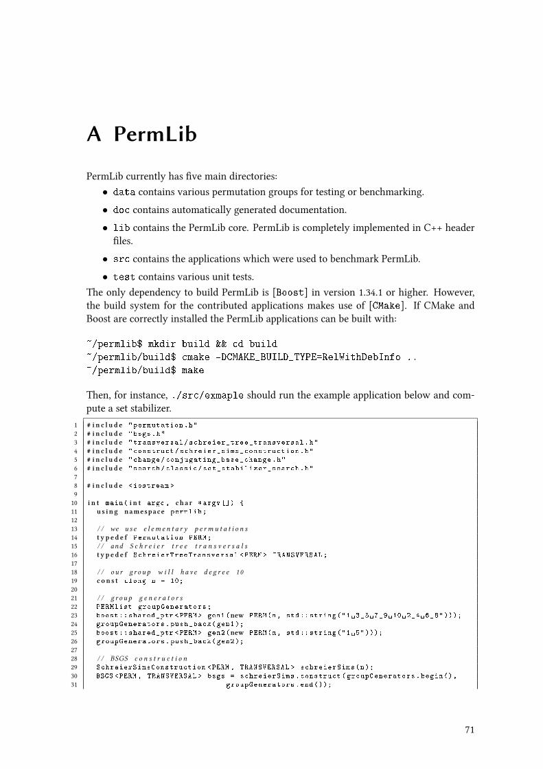
A PermLib
PermLib currently has Vve main directories:
• data contains various permutation groups for testing or benchmarking.
• doc contains automatically generated documentation.
• lib contains the PermLib core. PermLib is completely implemented in C++ headerVles.
• src contains the applications which were used to benchmark PermLib.
• test contains various unit tests.
The only dependency to build PermLib is [Boost] in version 1.34.1 or higher. However,the build system for the contributed applications makes use of [CMake]. If CMake andBoost are correctly installed the PermLib applications can be built with:
~/permlib$ mkdir build && cd build
~/permlib/build$ cmake -DCMAKE_BUILD_TYPE=RelWithDebInfo ..
~/permlib/build$ make
Then, for instance, ./src/exmaple should run the example application below and com-pute a set stabilizer.
1 # i n c l u d e "permutation.h"
2 # i n c l u d e "bsgs.h"
3 # i n c l u d e "transversal/schreier_tree_transversal.h"
4 # i n c l u d e "construct/schreier_sims_construction.h"
5 # i n c l u d e "change/conjugating_base_change.h"
6 # i n c l u d e "search/classic/set_stabilizer_search.h"
78 # i n c l u d e <iostream >
910 i n t main( i n t argc , cha r *argv [])
11 u s i n g namespace permlib;
1213 / / we u s e e l e m e n t a r y p e r m u t a t i o n s14 t y p e d e f Permutation PERM;
15 / / and S c h r e i e r t r e e t r a n s v e r s a l s16 t y p e d e f SchreierTreeTransversal <PERM > TRANSVERSAL;
1718 / / o u r g r o u p w i l l h a v e d e g r e e 1 019 c o n s t ulong n = 10;
2021 / / g r o u p g e n e r a t o r s22 PERMlist groupGenerators;
23 boost::shared_ptr <PERM > gen1(new PERM(n, std:: string("1 3 5 7 9 10 2 4 6 8")));
24 groupGenerators.push_back(gen1);
25 boost::shared_ptr <PERM > gen2(new PERM(n, std:: string("1 5")));
26 groupGenerators.push_back(gen2);
2728 / / BSGS c o n s t r u c t i o n29 SchreierSimsConstruction <PERM , TRANSVERSAL > schreierSims(n);
30 BSGS <PERM , TRANSVERSAL > bsgs = schreierSims.construct(groupGenerators.begin(),
31 groupGenerators.end ());
71

A PermLib
32 std::cout << "Group " << bsgs << std::endl;
3334 / / we want t o s t a b i l i z e a s e t35 c o n s t ulong DeltaSize = 4;
36 c o n s t ulong Delta[DeltaSize] = 0, 4, 7, 8;
3738 / / c h an g e t h e b a s e s o t h a t i s p r e f i x e d by t h e s e t39 ConjugatingBaseChange <PERM ,TRANSVERSAL ,
40 RandomBaseTranspose <PERM ,TRANSVERSAL > > baseChange(bsgs);
41 baseChange.change(bsgs , Delta , Delta+DeltaSize );
4243 / / p r e p a r e s e a r c h w i t h o u t DCM p r u n i n g44 classic :: SetStabilizerSearch <PERM ,TRANSVERSAL > backtrackSearch(bsgs , 0);
45 backtrackSearch.construct(Delta , Delta+DeltaSize );
4647 / / s t a r t t h e s e a r c h48 BSGS <PERM ,TRANSVERSAL > stabilizer(n);
49 backtrackSearch.search(stabilizer );
5051 std::cout << "Stabilizer " << stabilizer << std::endl;
5253 r e t u r n 0;
54
72
Nomenclature
() identity permutation, page 3
αG orbit of α ∈ Ω under g ∈ G, page 3
αg action of g ∈ G on α ∈ Ω, page 3
cosetn the coset which a node n of a search tree corresponds to, page 27
∆(i) i-th fundamental orbit, page 6
fix Π ordered sequence of single-element cells of a partition Π in the order in which theyappeared in the reVnement process, page 39
intersect intersection of a partition with a set, page 51
g− inverse of g ∈ G, page 3
log logarithm to base 2, page 6
|G : H| index of H in G, page 3
|G| order of group G, page 3
ΩP(n) child restriction in classical backtrack search of node n depending on property P ,page 31
OP(Ω) set of all ordered partitions of Ω, page 37
Π ∧ Σ intersection of two partitions Π, Σ, page 37
U(G) uniform distribution on the set or group G, page 19
G[i] pointwise stabilizer of the i− 1 Vrst base elements, page 5
G(α1,...,αk) pointwise stabilizer of (α1, . . . , αk) as a tuple, page 4
Gα1,...,αk setwise stabilizer of α1, . . . , αk as a set, page 4
Sg conjugate of S ⊆ G under g ∈ G, page 21
Sn the symmetric group of n elements, page 4
73
References
Bibliography
[Bab91] László Babai. Local expansion of vertex-transitive graphs and random gen-eration in Vnite groups. In STOC ’91: Proceedings of the twenty-third annualACM symposium on Theory of computing, pages 164–174, New York, NY, USA,1991. ACM.
[BL85] Gregory Butler and Clement W. H. Lam. A general backtrack algorithm forthe isomorphism problem of combinatorial objects. Journal of Symbolic Com-putation, 1(4):363–381, 1985.
[Bri00] Gunnar Brinkmann. Isomorphism rejection in structure generation programs.In Discrete Mathematical Chemistry. DIMACS Series in Discrete Mathematicaland Theoretical Computer Science, volume 51, pages 25–38. American Mathe-matical Society, 2000.
[BSS09] David Bremner, Mathieu Dutour Sikiric, and Achill Schürmann. Polyhedralrepresentation conversion up to symmetries. In David Avis, David Bremner,and Antoine Deza, editors, Polyhedral computation, CRM Proceedings & Lec-ture Notes, pages 45–72. American Mathematical Society, 2009. Available fromWorld Wide Web: http://arxiv.org/abs/math/0702239.
[But91] Gregory Butler. Fundamental algorithms for permutation groups. Springer,1991.
[CH92] John J. Cannon and George Havas. Algorithms for groups. Australian Com-puter Journal, 24(2):51–60, 1992.
[CLRS09] Thomas H. Cormen, Charles E. Leiserson, Ronald L. Rivest, and CliUord Stein.Introduction to Algorithms. The MIT Press, 3rd edition, 2009.
[CST89] Peter J. Cameron, Ron Solomon, and Alexandre Turull. Chains of subgroupsin symmetric groups. Journal of Algebra, (127):340–352, 1989.
[HEO05] Derek F. Holt, Bettina Eick, and Eamonn A. O’Brien. Handbook of Compu-tational Group Theory. Discrete Mathematics and Applications. Chapman &Hall/CRC, 2005.
[Jun03] Tommi Junttila. On the symmetry reduction method for petri nets and similarformalisms. Research Report A80, Helsinki University of Technology, Labora-tory for Theoretical Computer Science, Espoo, Finland, September 2003.
[Ker99] Adalbert Kerber. Applied Finite Group Actions. Algorithms and Combina-torics. Springer, 2nd edition, 1999.
74
[Knu91] Donald E. Knuth. EXcient representation of perm groups. Combinatorica,11(1):33–43, 1991.
[Knu98] Donald E. Knuth. The art of computer programming, volume 3: sorting andsearching. Addison Wesley, 2nd edition, 1998.
[KÖ06] Petteri Kaski and Patric R.J. Östergård. ClassiVcation Algorithms for Codes andDesigns, volume 15 of Algorithms and Computation in Mathematics. Springer,2006.
[Leo80] JeUrey S. Leon. On an algorithm for Vnding a base and a strong generating setfor a group given by generating permutations. Mathematics of Computation,35(151):941–974, July 1980. Available from World Wide Web: http://www.jstor.org/pss/2006206.
[Leo84] JeUrey S. Leon. Computing automorphism groups of combinatorial objects.In Computational group theory (Durham, 1982), pages 321–335, London, 1984.Academic Press.
[Leo91] JeUrey S. Leon. Permutation group algorithms based on partitions, I: Theoryand algorithms. Journal of Symbolic Computation, 12:533–583, 1991.
[Leo97] JeUrey S. Leon. Partitions, reVnements, and permutation group computation.In Larry Finkelstein and William M. Kantor, editors, Groups and computa-tion II, volume 28 of DIMACS Series in Discrete Mathematics and Theoreti-cal Computer Science, pages 123–158. American Mathematical Society, Provi-dence, R.I., 1997.
[Luk93] Eugene M. Luks. Permutation groups and polynomial-time computing. InGroups and Computation, DIMACS series in Discrete Mathematics and Theo-retical Computer Science, volume 11, pages 139–175. American MathematicalSociety, 1993.
[Mar09] François Margot. 50 Years of Integer Programming 1958-2008, chapter Symme-try in Integer Linear Programming, pages 647–686. Springer, 2009.
[McK81] Brendan D. McKay. Practical graph isomorphism. Congressus Numerantium,30:45–87, 1981. Available from World Wide Web: http://cs.anu.edu.au/~bdm/papers/pgi.pdf.
[McK98] Brendan D. McKay. Isomorph-free exhaustive generation. Journal of Al-gorithms, 26(2):306–324, 1998. Available from World Wide Web: http:
//cs.anu.edu.au/~bdm/papers/orderly.pdf.
[Mila] Wiki of Robert L.Miller. Available from World Wide Web: http://wiki.rlmiller.org/PermutationGroups. [Online; accessed January 10, 2010].
[Milb] Robert L. Miller. rlm-blog. Available from World Wide Web: http://blog.rlmiller.org/. [Online; accessed January 10, 2010].
[Ser03] Ákos Seress. Permutation Group Algorithms. Cambridge University Press,2003.
[Sim70] Charles C. Sims. Computational methods in the study of permutation groups.In John Leech, editor, Computational Problems in Abstract Algebra, pages 169–183. Pergamon Press, 1970.
75

A PermLib
[Sim71a] Charles C. Sims. Computation with permutation groups. In SYMSAC ’71:Proceedings of the second ACM symposium on Symbolic and algebraic manip-ulation, pages 23–28, New York, NY, USA, 1971. ACM.
[Sim71b] Charles C. Sims. Determining the conjugacy classes of a permutation group.In Garrett BirkhoU and Marshall Hall Jr., editors, Computers in Algebra andNumber Theory, volume 4 of SIAM-AMS Proceedings, pages 191–195, Provi-dence, R.I., 1971. American Mathematical Society.
[The97] Heiko Theißen. Eine Methode zur Normalisatorberechnung in Permutation-sgruppen mit Anwendungen in der Konstruktion primitiver Gruppen, vol-ume 21 of Aachener Beiträge zur Mathematik. Verlag der Augustiner Buch-handlung, 1997. Ph.D. thesis at RWTH Aachen.
[Zie95] Günter M. Ziegler. Lectures on polytopes. Springer, New York, 1995.
Software
[Boost] Boost free peer-reviewed portable C++ source libraries. http://www.boost.org/.
[CMake] CMake – Cross Platform Make. http://www.cmake.org/.
[GAP] GAP – Groups, Algorithms, Programming – a System for Computational Dis-crete Algebra. http://www.gap-system.org/.
[GUAVA] GUAVA – a GAP package for computing with error-correcting codes. http:
//www.gap-system.org/Packages/guava.html.
[Magma] MAGMA Computational Algebra System. http://magma.maths.usyd.edu.au/.
[nauty] nauty, computing automorphism groups of graphs and digraphs. http://cs.anu.edu.au/~bdm/nauty/.
[Sage] Sage Mathematics Software. http://www.sagemath.org/.
[Vgrind] Valgrind – a GPL’d system for debugging and proVling Linux programs. http://valgrind.org/.
76
Index
backtrack reVnement, 38, 39base, 5
change, 17, 58, 67construction, 11, 53, 67nonredundant, 5, 6
base point transposition, 17, 57, 67BSGS, 6
coset, 3cyclic group, 7, 8, 14, 28
degree of a group, 3double coset, 3
minimality, 30, 46, 62, 65, 67
fundamental orbit, 53
GAP, 1, 14, 49, 50, 53, 67group
degree, 3order, 3
index, 3, 6
Lagrange’s Theorem, 3, 6
Magma, 1, 14, 49, 62, 67, 68
orbit, 3construction, 7fundamental orbit, 6
order of a group, 3
P-reVnement, 37, 39, 43, 47extension to cosets, 47group membership, 44set image, 47set stabilizer, 43
partition, 37, 51discrete, 38Vx points, 39, 45intersection, 37, 38, 51
reVnement, 37, 38permutation, 2–3
cycle form, 2elementary, 49, 67permutation word, 49
R-base, 39, 40, 43set stabilizer, 44
Schreier generator, 11, 18trivial by deVnition, 12, 18
Schreier tree, 8, 14, 67shallow, 14–17, 67
Schreier vector, 8Schreier-Sims algorithm, 11
complexity, 13randomized, 21
search treeclassical backtracking, 27partition backtracking, 40
SGS, see strong generating setsiftee, 10sifting, 10stabilizer, 4
pointwise, 4setwise, 4
stabilizer chain, 5, 6, 29strong generating set, 6–7
for subgroup, 29, 45symmetric group, 6, 7, 53, 55, 63
transposition, see base point transpositiontransversal, 3, 6
explicit, 9Schreier tree, see Schreier tree
77

INDEX
78