Fundamentals of Rheology:

1 Introduction:

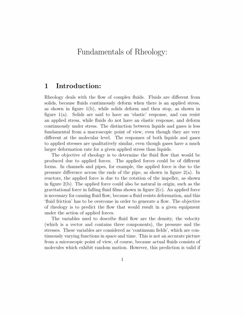
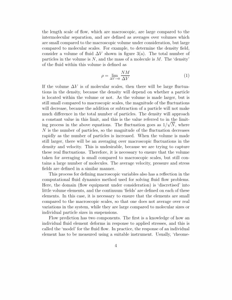
Rheology deals with the flow of complex fluids. Fluids are different fromsolids, because fluids continuously deform when there is an applied stress,as shown in figure 1(b), while solids deform and then stop, as shown infigure 1(a). Solids are said to have an ‘elastic’ response, and can resistan applied stress, while fluids do not have an elastic response, and deformcontinuously under stress. The distinction between liquids and gases is lessfundamental from a macroscopic point of view, even though they are verydifferent at the molecular level. The responses of both liquids and gasesto applied stresses are qualitatively similar, even though gases have a muchlarger deformation rate for a given applied stress than liquids.

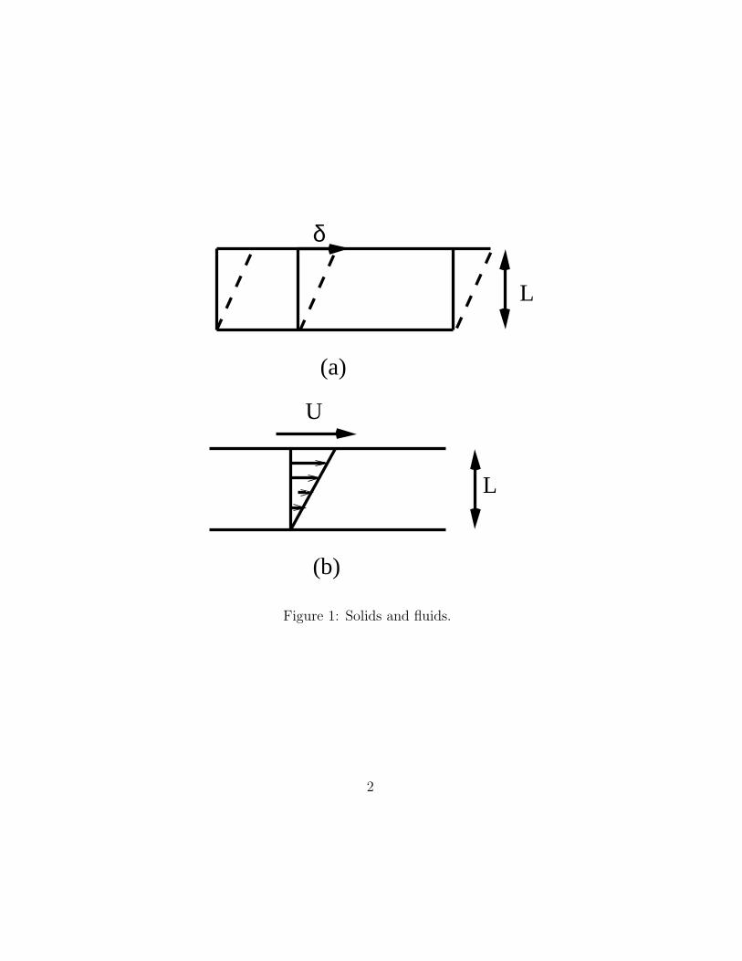
The objective of rheology is to determine the fluid flow that would beproduced due to applied forces. The applied forces could be of differentforms. In channels and pipes, for example, the applied force is due to thepressure difference across the ends of the pipe, as shown in figure 2(a). Inreactors, the applied force is due to the rotation of the impeller, as shownin figure 2(b). The applied force could also be natural in origin, such as thegravitational force in falling fluid films shown in figure 2(c). An applied forceis necessary for causing fluid flow, because a fluid resists deformation, and this‘fluid friction’ has to be overcome in order to generate a flow. The objectiveof rheology is to predict the flow that would result in a given equipmentunder the action of applied forces.

The variables used to describe fluid flow are the density, the velocity(which is a vector and contains three components), the pressure and thestresses. These variables are considered as ‘continuum fields’, which are con-tinuously varying functions in space and time. This is not an accurate picturefrom a microscopic point of view, of course, because actual fluids consists ofmolecules which exhibit random motion. However, this prediction is valid if

1

U

L

(b)

L

δ

(a)

Figure 1: Solids and fluids.

2

Motor

Liquid level

Shaft

Impeller

(c)

(a)

(b)

Figure 2: Types of external forces.

3

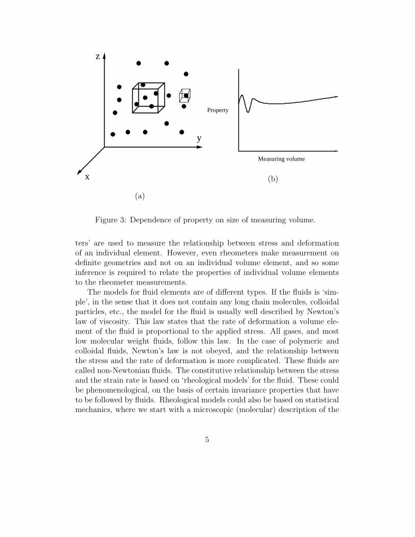
the length scale of flow, which are macroscopic, are large compared to theintermolecular separation, and are defined as averages over volumes whichare small compared to the macroscopic volume under consideration, but largecompared to molecular scales. For example, to determine the density field,consider a volume of fluid ∆V shown in figure 3(a). The total number ofparticles in the volume is N , and the mass of a molecule is M . The ‘density’of the fluid within this volume is defined as

ρ = lim∆V →0

NM

∆V(1)

If the volume ∆V is of molecular scales, then there will be large fluctua-tions in the density, because the density will depend on whether a particleis located within the volume or not. As the volume is made larger, but isstill small compared to macroscopic scales, the magnitude of the fluctuationswill decrease, because the addition or subtraction of a particle will not makemuch difference in the total number of particles. The density will approacha constant value in this limit, and this is the value referred to in the limit-ing process in the above equations. The fluctuation goes as 1/

√N , where

N is the number of particles, so the magnitude of the fluctuation decreasesrapidly as the number of particles is increased. When the volume is madestill larger, there will be an averaging over macroscopic fluctuations in thedensity and velocity. This is undesirable, because we are trying to capturethese real fluctuations. Therefore, it is necessary to ensure that the volumetaken for averaging is small compared to macroscopic scales, but still con-tains a large number of molecules. The average velocity, pressure and stressfields are defined in a similar manner.

This process for defining macroscopic variables also has a reflection in thecomputational fluid dynamics method used for solving fluid flow problems.Here, the domain (flow equipment under consideration) is ‘discretised’ intolittle volume elements, and the continuum ‘fields’ are defined on each of theseelements. In this case, it is necessary to ensure that the elements are smallcompared to the macroscopic scales, so that one does not average over realvariations in the system, while they are large compared to molecular sizes orindividual particle sizes in suspensions.

Flow prediction has two components. The first is a knowledge of how anindividual fluid element deforms in response to applied stresses, and this iscalled the ‘model’ for the fluid flow. In practice, the response of an individualelement has to be measured using a suitable instrument. Usually, ‘rheome-

4

x

y

z

(a)

Property

Measuring volume

(b)

Figure 3: Dependence of property on size of measuring volume.

ters’ are used to measure the relationship between stress and deformationof an individual element. However, even rheometers make measurement ondefinite geometries and not on an individual volume element, and so someinference is required to relate the properties of individual volume elementsto the rheometer measurements.

The models for fluid elements are of different types. If the fluids is ‘sim-ple’, in the sense that it does not contain any long chain molecules, colloidalparticles, etc., the model for the fluid is usually well described by Newton’slaw of viscosity. This law states that the rate of deformation a volume ele-ment of the fluid is proportional to the applied stress. All gases, and mostlow molecular weight fluids, follow this law. In the case of polymeric andcolloidal fluids, Newton’s law is not obeyed, and the relationship betweenthe stress and the rate of deformation is more complicated. These fluids arecalled non-Newtonian fluids. The constitutive relationship between the stressand the strain rate is based on ‘rheological models’ for the fluid. These couldbe phenomenological, on the basis of certain invariance properties that haveto be followed by fluids. Rheological models could also be based on statisticalmechanics, where we start with a microscopic (molecular) description of the

5

fluid, and use averaging to obtain the average properties.Once we have a relationship between the rate of deformation and the

applied stresses, it is necessary to determine how the velocity field in thefluid varies with position and time. This is usually determined using a com-bination of the fluid model, usually called the constitutive equation, and theconservation equations for the mass and momentum (Newton’s laws). Thelaw of conservation of mass states that mass can neither be created or de-stroyed, and the law of conservation of momentum states that the rate ofchange of momentum is equal to the sum of the applied forces. These arecombined with the constitutive relations to provide a set of equations whichdescribe the variation of the fluid density and velocity fields with positionand time.

There are two broad approaches for determining the velocity, density andother dynamical quantities within the equipment of interest from a knowl-edge of the variation of the properties in space and time. The first is touse analytical techniques, which involve integration of the equations using asuitable mathematical technique. The second is computational, where thedifferential equations are ‘discretised’ and solved on the computer. We shallnot go into the details of either of these solution techniques here, but merelysketch how the solution is determined for simple problems.

The above solution procedure seems simple enough, and one might expectthat once the fluid properties are known, the flow properties can easily becalculated with the aid of a suitable computer. However, there are numerouscomplications.

1. The dynamical properties of the fluid (the constitutive relation) maynot be well known. This is common in polymeric and colloidal sys-tems, where the stress depends in a complicated way on the rate ofdeformation. In such cases, it is necessary to have a good understand-ing between the dynamical properties of the fluid and the underlyingmicrostructure.

2. The flow may be turbulent. In a ‘laminar’ flow, the streamlines aresmooth and vary slowly with position, so that the deformation of anyfluid element resembles the deformation that would be observed in atest equipment which contained only that element. However, when theflow becomes turbulent, the streamlines assume a chaotic form and theflow is highly irregular. Therefore, the flow of an individual volumeelement does not resemble the deformation that would be observed

6

in a test sample containing only that element. More sophisticatedtechniques are required to analyse turbulent flows.

3. The flow may actually be too complicated to solve even on a computer.This is especially true of complicated equipments such as extruders,mixers, fluidised beds, etc. In this case, it is necessary to have alterna-tive techniques to handle these problems.

An important consideration in fluid flow problems is the ‘Reynolds num-ber’, which provides the ratio of inertial and viscous effects. Fluid ‘iner-tia’ refers to the change in momentum due to acceleration, while ‘viscouseffects’ refers to the change in momentum due to frictional forces exerteddue to fluid deformation. The Reynolds number is a dimensionless numberRe = (ρUL/η), where ρ and η are the fluid viscosity and density, U is the ve-locity and L is the characteristic length of the flow equipment. The Reynoldsnumber can also be considered as a ratio between ‘convective’ and ‘diffusive’effects, where the ‘convective’ effect refers to the transport of momentumdue to the motion of fluid elements, while the ‘diffusive’ effect refers to thetransport of momentum due to frictional stresses within the fluid. When theReynolds number is small, viscous effects are dominant and the dominantmechanism of momentum transport is due to diffusion. When the Reynoldsnumber is large, it is expected that viscous effects can be neglected. In flowsof complex fluids that we will be concerned with, the Reynolds number is usu-ally sufficiently small that inertial effects can be neglected. Therefore, theseflows are mostly dominated by viscosity, and turbulence is not encountered.

2 Concept of viscosity

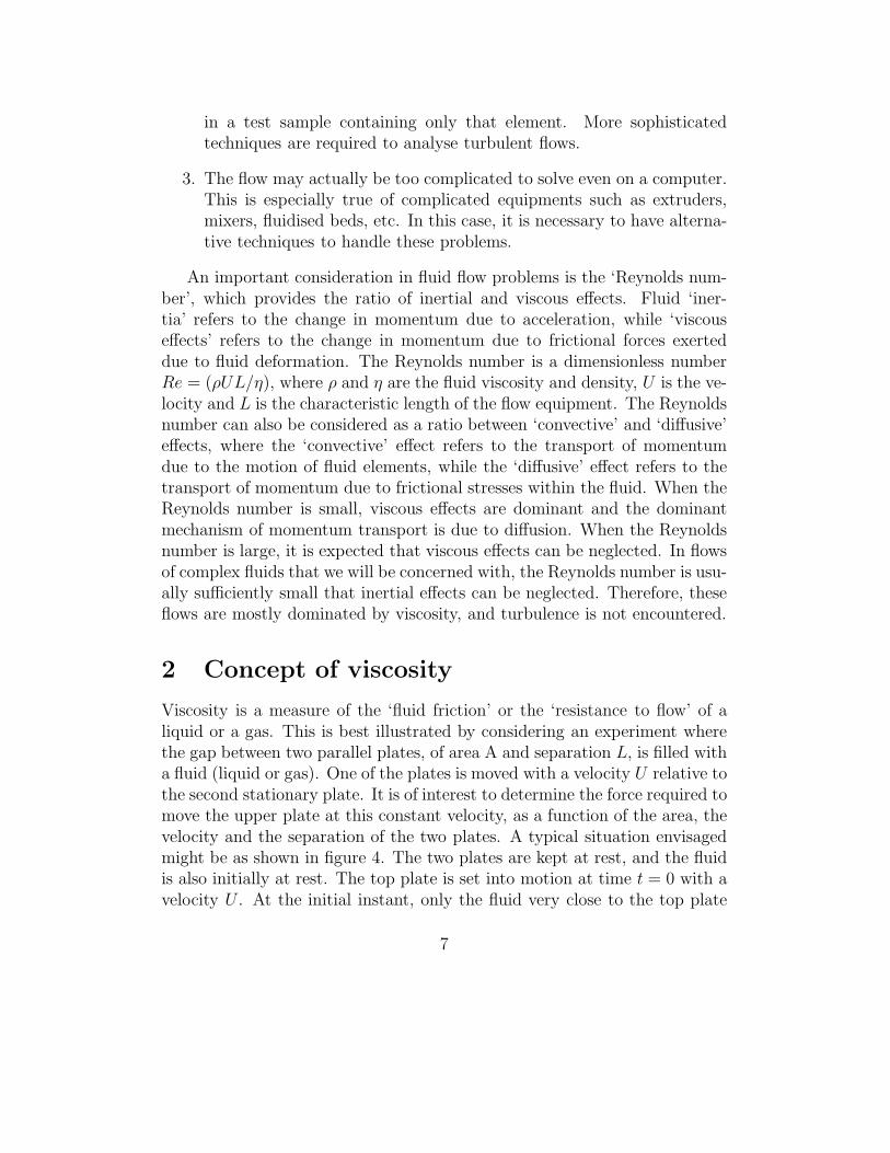
Viscosity is a measure of the ‘fluid friction’ or the ‘resistance to flow’ of aliquid or a gas. This is best illustrated by considering an experiment wherethe gap between two parallel plates, of area A and separation L, is filled witha fluid (liquid or gas). One of the plates is moved with a velocity U relative tothe second stationary plate. It is of interest to determine the force required tomove the upper plate at this constant velocity, as a function of the area, thevelocity and the separation of the two plates. A typical situation envisagedmight be as shown in figure 4. The two plates are kept at rest, and the fluidis also initially at rest. The top plate is set into motion at time t = 0 with avelocity U . At the initial instant, only the fluid very close to the top plate

7

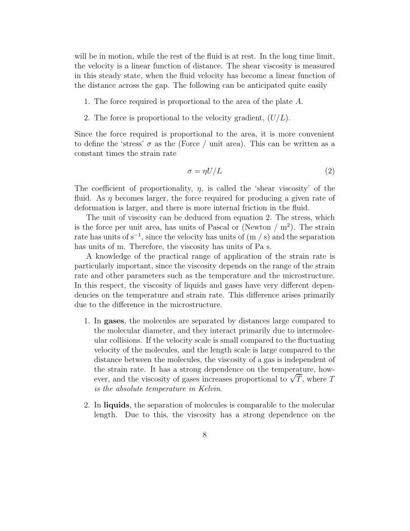
will be in motion, while the rest of the fluid is at rest. In the long time limit,the velocity is a linear function of distance. The shear viscosity is measuredin this steady state, when the fluid velocity has become a linear function ofthe distance across the gap. The following can be anticipated quite easily

1. The force required is proportional to the area of the plate A.

2. The force is proportional to the velocity gradient, (U/L).

Since the force required is proportional to the area, it is more convenientto define the ‘stress’ σ as the (Force / unit area). This can be written as aconstant times the strain rate

σ = ηU/L (2)

The coefficient of proportionality, η, is called the ‘shear viscosity’ of thefluid. As η becomes larger, the force required for producing a given rate ofdeformation is larger, and there is more internal friction in the fluid.

The unit of viscosity can be deduced from equation 2. The stress, whichis the force per unit area, has units of Pascal or (Newton / m2). The strainrate has units of s−1, since the velocity has units of (m / s) and the separationhas units of m. Therefore, the viscosity has units of Pa s.

A knowledge of the practical range of application of the strain rate isparticularly important, since the viscosity depends on the range of the strainrate and other parameters such as the temperature and the microstructure.In this respect, the viscosity of liquids and gases have very different depen-dencies on the temperature and strain rate. This difference arises primarilydue to the difference in the microstructure.

1. In gases, the molecules are separated by distances large compared tothe molecular diameter, and they interact primarily due to intermolec-ular collisions. If the velocity scale is small compared to the fluctuatingvelocity of the molecules, and the length scale is large compared to thedistance between the molecules, the viscosity of a gas is independent ofthe strain rate. It has a strong dependence on the temperature, how-ever, and the viscosity of gases increases proportional to

√T , where T

is the absolute temperature in Kelvin.

2. In liquids, the separation of molecules is comparable to the molecularlength. Due to this, the viscosity has a strong dependence on the

8

U

L

U

L

U

L

Figure 4: Development of a steady flow in a channel between two platesseparated by a distance L when one of the plates is moved with a velocity U .

9

temperature, as well as the strain rate. The flow of a liquid takesplace due to the sliding of layers of the liquid past each other, and thissliding is easier when the temperature is higher and the molecules havea higher fluctuating velocity. Thus, the viscosity typically decreaseswith increase in temperature. However, the dependence on the strainrate can be quite complex.

2.1 Temperature dependence

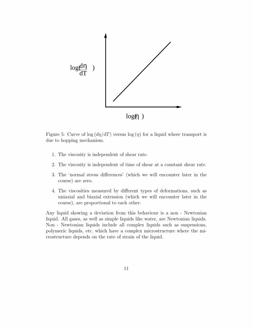
The viscosity of Newtonian liquids decreases with an increase in tempera-ture, according to an Arrhenius relationship. The reason for this kind ofrelationship is not quite clear. However, it is thought that relative motionbetween the different molecules in a fluid is due to a type of activated ‘hop-ping’ mechanism, and so the viscosity of a liquid also obeys an Arrheniustype behaviour.

η = A exp (−B/T ) (3)

where T is the absolute temperature (Kelvin) and A and B are constantsof the liquids. The constant B can be determined by plotting log (dη/dT )versus log η, as shown in figure 5. This curve has a slope of (B/T 2), whereT is the absolute temperature. The temperature dependence is strongerfor liquids with greater viscosity, and under normal conditions the thumbrule is that the viscosity decreases by about 3 % for every degree rise inthe temperature. Consequently, it is important to be able to maintain thetemperature a constant in viscometric measurements. This is of particularimportance because the shear of a liquid results in viscous heating, whichcould change the temperature. Therefore, in a practical measurement, carehas to be taken to ensure that sufficient heat is extracted to maintain thesystem at a steady temperature.

The viscosity of liquids increases exponentially with pressure. However,this dependence is not very strong for pressure variations of the order of afew bar, and so is usually ignored in practical applications.

2.2 Dependence on shear rate

The shear rate dependence of fluids is an important consideration, since manyfluids have complex shear rate dependence. It is first important to make adistinction between simple ‘Newtonian’ fluids and ‘non - Newtonian’ fluids.Newtonian fluids are characterised by the following behaviour:

10

log( )

log( )

η

dηdT

Figure 5: Curve of log (dη/dT ) versus log (η) for a liquid where transport isdue to hopping mechanism.

1. The viscosity is independent of shear rate.

2. The viscosity is independent of time of shear at a constant shear rate.

3. The ‘normal stress differences’ (which we will encounter later in thecourse) are zero.

4. The viscosities measured by different types of deformations, such asuniaxial and biaxial extension (which we will encounter later in thecourse), are proportional to each other.

Any liquid showing a deviation from this behaviour is a non - Newtonianliquid. All gases, as well as simple liquids like water, are Newtonian liquids.Non - Newtonian liquids include all complex liquids such as suspensions,polymeric liquids, etc. which have a complex microstructure where the mi-crostructure depends on the rate of strain of the liquid.

11

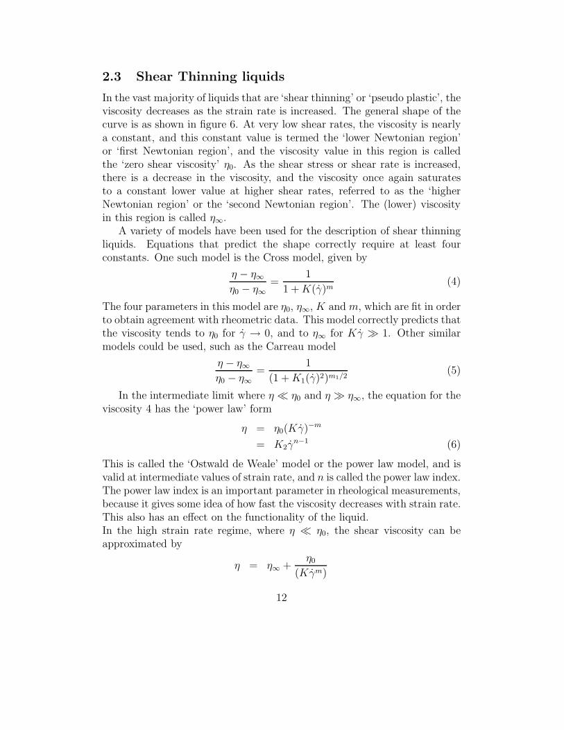
2.3 Shear Thinning liquids

In the vast majority of liquids that are ‘shear thinning’ or ‘pseudo plastic’, theviscosity decreases as the strain rate is increased. The general shape of thecurve is as shown in figure 6. At very low shear rates, the viscosity is nearlya constant, and this constant value is termed the ‘lower Newtonian region’or ‘first Newtonian region’, and the viscosity value in this region is calledthe ‘zero shear viscosity’ η0. As the shear stress or shear rate is increased,there is a decrease in the viscosity, and the viscosity once again saturatesto a constant lower value at higher shear rates, referred to as the ‘higherNewtonian region’ or the ‘second Newtonian region’. The (lower) viscosityin this region is called η∞.

A variety of models have been used for the description of shear thinningliquids. Equations that predict the shape correctly require at least fourconstants. One such model is the Cross model, given by

η − η∞η0 − η∞

=1

1 + K(γ̇)m(4)

The four parameters in this model are η0, η∞, K and m, which are fit in orderto obtain agreement with rheometric data. This model correctly predicts thatthe viscosity tends to η0 for γ̇ → 0, and to η∞ for Kγ̇ ≫ 1. Other similarmodels could be used, such as the Carreau model

η − η∞η0 − η∞

=1

(1 + K1(γ̇)2)m1/2(5)

In the intermediate limit where η ≪ η0 and η ≫ η∞, the equation for theviscosity 4 has the ‘power law’ form

η = η0(Kγ̇)−m

= K2γ̇n−1 (6)

This is called the ‘Ostwald de Weale’ model or the power law model, and isvalid at intermediate values of strain rate, and n is called the power law index.The power law index is an important parameter in rheological measurements,because it gives some idea of how fast the viscosity decreases with strain rate.This also has an effect on the functionality of the liquid.In the high strain rate regime, where η ≪ η0, the shear viscosity can beapproximated by

η = η∞ +η0

(Kγ̇m)

12

Shear stress

Vis

cosi

ty

Shear rate

Shear rate

Vis

cosi

tySh

ear

stre

ss

Figure 6: Typical plots of stress, strain and viscosity (all on log scales) for ashear thinning fluid.

13

= η∞ + K2γ̇n−1 (7)

If we set n equal to zero in the above equation, we obtain

η = η∞ +K2

γ̇(8)

When inserted into the stress - strain relationship, this yields

σ = σ0 + ηpγ̇ (9)

where σ0 is the yield stress in the Bingham model.

2.4 Shear thickening liquids

There are some liquids whose viscosity increases as the shear rate is in-creased. Concentrated suspensions, for example, could show shear thickeningbehaviour because the particles form sample spanning clusters. This couldalso result from flocculation of particles due to shear, or due to the jammingof high aspect ratio particles due to rotation by the shear flow. These areusually represented by power - law relations with exponent n greater than 1.

2.5 Time effects

In most fluids which display a shear thinning, there is also a decrease of theviscosity in time at a constant strain rate. This is because of the gradualbreakdown of the viscosity under stress, and is similar to the mechanism forshear thickening. There could be a recovery of the structure upon cessationof stress, and the time scale for the recovery gives the typical time for thestructures to recover. This type of recovery is typically observed in polymersolutions. There are other cases where the breaking down of bonds is irre-versible, such as polymer gels. Here, the viscosity will not recover after thestress has been removed. There are still other cases, such as liquid crystals,where the structures do not break down irreversibly, but the recovery time islong compared to any processing time scale. In this case, also there will notbe any recovery on the time scale of observation, and the change in structurewill appear irreversible.

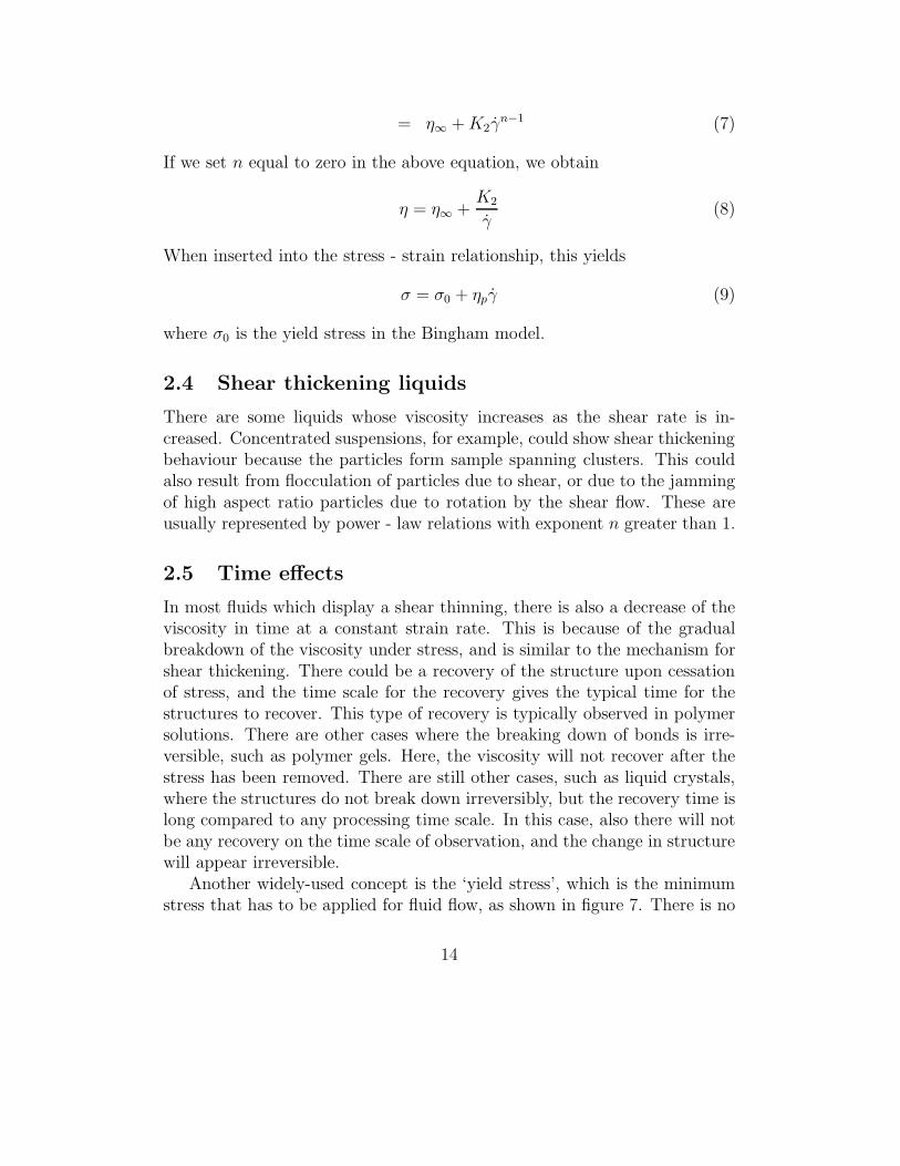
Another widely-used concept is the ‘yield stress’, which is the minimumstress that has to be applied for fluid flow, as shown in figure 7. There is no

14

γ.

σB

AC

D

σy

Figure 7: The shear stress versus strain rate for Newtonian (A), shear thin-ning (B), shear thickening (C) and yield stress (D) fluids.

15

flow for σ < σy, and the fluid starts to flow only for σ < σy. The constitutiverelation for a yield-stress fluid is usually written as,

σ = σy + ηγ̇ for σ > σy (10)

However, the concept of yield stress should be used with caution, since theyield stress often depends on the time for which the stress is applied. Amaterial which is rigid for a short duration will flow if stress is continuouslyapplied for a much longer duration.

The apparent viscosity of a fluid could also depend on the duration ofthe applied stress, when the strain rate is maintained a constant. In the caseof thixotropic substances, the shear stress decreases with time at a constantstrain rate. In contrast, the shear stress of rheopectic substances increaseswith time at constant shear rate.

3 Visco-elasticity:

The term ‘linear viscoelasticity’ refers to the relation between stress anddeformation of a material near equilibrium when the deformation is small.Deformations are not usually small under conditions of processing or use, andso data obtained by linear viscoelasticity measurements often do not have di-rect relevance to conditions of use. However, these tests are important for tworeasons. First, these tests are easier to carry out and understand than non -linear measurements, and the parameters obtained from linear viscoelastic-ity measurements are a reliable reflection of the state of the system. Second,these measurements can also be used quality control, and any variations inquality can be easily detected by linear viscoelasticity measurements.

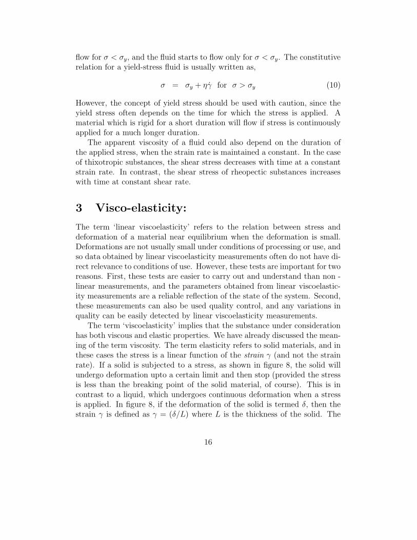
The term ‘viscoelasticity’ implies that the substance under considerationhas both viscous and elastic properties. We have already discussed the mean-ing of the term viscosity. The term elasticity refers to solid materials, and inthese cases the stress is a linear function of the strain γ (and not the strainrate). If a solid is subjected to a stress, as shown in figure 8, the solid willundergo deformation upto a certain limit and then stop (provided the stressis less than the breaking point of the solid material, of course). This is incontrast to a liquid, which undergoes continuous deformation when a stressis applied. In figure 8, if the deformation of the solid is termed δ, then thestrain γ is defined as γ = (δ/L) where L is the thickness of the solid. The

16

σ

L

δ

Figure 8: Displacement due to the stress in a solid.

force required to produce this displacement is proportional to the cross sec-tional area A, and the stress (force per unit area) is related to the strain fieldby

σ =Gδ

L(11)

where G is the ‘modulus of elasticity’.It is useful to compare the quantity ‘strain’ used in the definition of

elasticity and ‘rate of strain’ used to define the viscosity. In figure 8, thevelocity of the top plate is the rate of change of the displacement with time.

U =dδ

dt(12)

Since the distance between the plates is a constant, the rate of strain is justthe time derivative of the strain

γ̇ =dγ

dt(13)

A ‘viscoelastic’ fluid is one which has both viscous and elastic properties, i.e. where a part of the stress is due to the strain field and another part is dueto the strain rate.

Next, we turn to the term ‘linear’ in the title ‘linear viscoelasticity’. Lin-ear just means that the relationship between the stress and the strain is alinear relationship, so that if the strain is increased by a factor of 2, the stressalso increases by a factor of 2. The Newton’s law of viscosity and equation

17

(11) for the elasticity are linear relationships. However, if we have a term ofthe form

σ = Kγ̇n (14)

it is easy to see that if the strain is increased by a constant factor, the stressdoes not increase by that factor. Therefore, the relationship is non - linear.Almost all non - Newtonian fluids have non - linear relationships between thestress and the strain rate, and therefore they cannot be described by linearviscoelastic theories. However, a linear relationship between the stress andstrain could be more complicated than the Newton’s law of viscosity, andcould include higher order time derivatives as well. For example

(

A3d3

dt3+ A2

d2

dt2+ A1

d

dt+ A0

)

σ =

(

B3d3

dt3+ B2

d2

dt2+ B1

d

dt+ B0

)

γ (15)

is a linear relationship between the stress and strain. Relations of the aboveform do not mean much unless we can relate them to viscous and elasticelements individually. This is the objective of linear viscoelasticity.

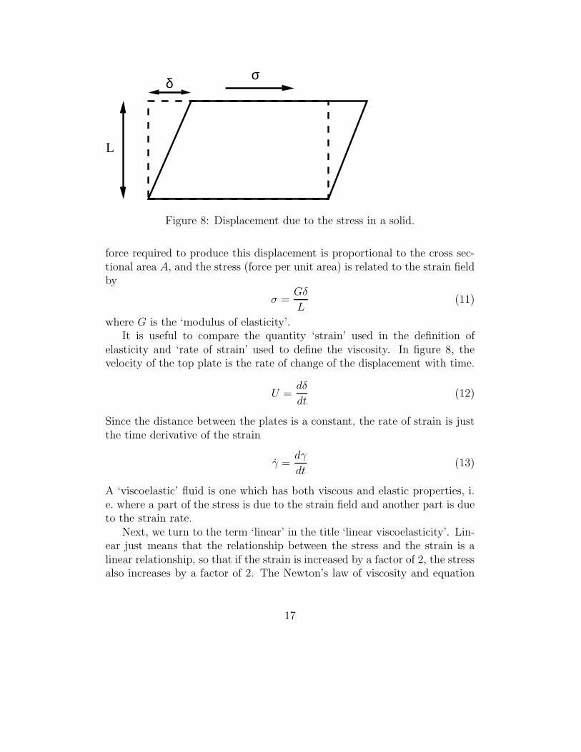
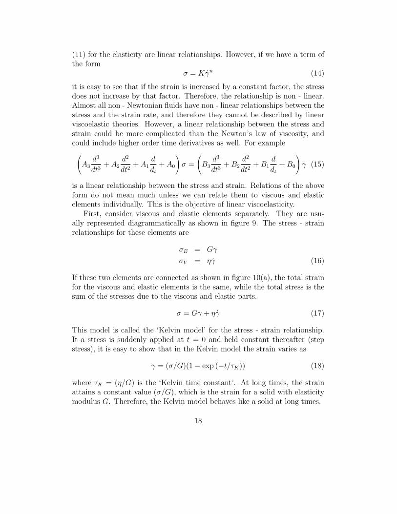
First, consider viscous and elastic elements separately. They are usu-ally represented diagrammatically as shown in figure 9. The stress - strainrelationships for these elements are

σE = Gγ

σV = ηγ̇ (16)

If these two elements are connected as shown in figure 10(a), the total strainfor the viscous and elastic elements is the same, while the total stress is thesum of the stresses due to the viscous and elastic parts.

σ = Gγ + ηγ̇ (17)

This model is called the ‘Kelvin model’ for the stress - strain relationship.It a stress is suddenly applied at t = 0 and held constant thereafter (stepstress), it is easy to show that in the Kelvin model the strain varies as

γ = (σ/G)(1 − exp (−t/τK)) (18)

where τK = (η/G) is the ‘Kelvin time constant’. At long times, the strainattains a constant value (σ/G), which is the strain for a solid with elasticitymodulus G. Therefore, the Kelvin model behaves like a solid at long times.

18

Figure 9: Elastic and viscous elements.

σσ v

σ

(a) (b)

γ

γ

e

e

v

Figure 10: Kelvin model (a) and Maxwell model (b) for the stress-strainrelationship.

19

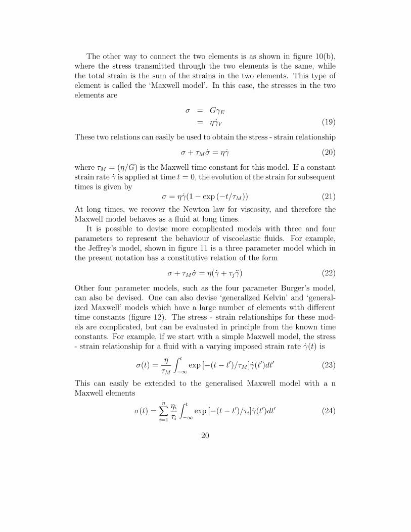
The other way to connect the two elements is as shown in figure 10(b),where the stress transmitted through the two elements is the same, whilethe total strain is the sum of the strains in the two elements. This type ofelement is called the ‘Maxwell model’. In this case, the stresses in the twoelements are

σ = GγE

= ηγ̇V (19)

These two relations can easily be used to obtain the stress - strain relationship

σ + τM σ̇ = ηγ̇ (20)

where τM = (η/G) is the Maxwell time constant for this model. If a constantstrain rate γ̇ is applied at time t = 0, the evolution of the strain for subsequenttimes is given by

σ = ηγ̇(1 − exp (−t/τM )) (21)

At long times, we recover the Newton law for viscosity, and therefore theMaxwell model behaves as a fluid at long times.

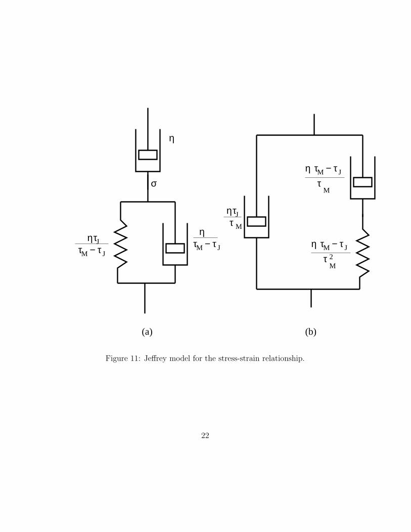
It is possible to devise more complicated models with three and fourparameters to represent the behaviour of viscoelastic fluids. For example,the Jeffrey’s model, shown in figure 11 is a three parameter model which inthe present notation has a constitutive relation of the form

σ + τM σ̇ = η(γ̇ + τjγ̈) (22)

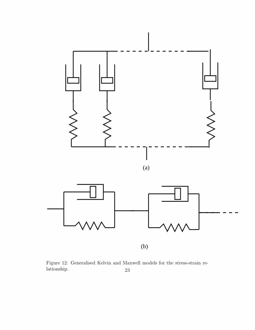
Other four parameter models, such as the four parameter Burger’s model,can also be devised. One can also devise ‘generalized Kelvin’ and ‘general-ized Maxwell’ models which have a large number of elements with differenttime constants (figure 12). The stress - strain relationships for these mod-els are complicated, but can be evaluated in principle from the known timeconstants. For example, if we start with a simple Maxwell model, the stress- strain relationship for a fluid with a varying imposed strain rate γ̇(t) is

σ(t) =η

τM

∫ t

−∞

exp [−(t − t′)/τM ]γ̇(t′)dt′ (23)

This can easily be extended to the generalised Maxwell model with a nMaxwell elements

σ(t) =n∑

i=1

ηi

τi

∫ t

−∞

exp [−(t − t′)/τi]γ̇(t′)dt′ (24)

20

where ηi and τi correspond to the ith Maxwell element. A similar relation-ship can be derived for the ‘generalised Kelvin’ model, where the strain isdetermined as a function of the applied stress. For a single Kelvin element,the relationship between the stress and strain is

γ(t) =1

η

∫ t

−∞

exp [−(t − t′)/τK ]σ(t′)dt′ (25)

For the generalised Kelvin model, this can easily be extended to provide arelaxation behaviour of the form

γ(t) =n∑

i=1

1

ηi

∫ t

−∞

exp [−(t − t′)/τi]σ(t′)dt′ (26)

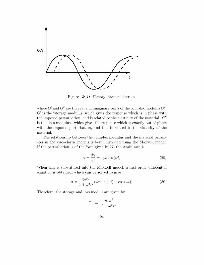
The above relationships are quite easy to derive once the models for theviscoelastic fluid are know. However, the basic question is how does onedetermine the model from a known relationship between the stress and strain.These model relationships are best derived using ‘oscillatory’ measurements,where a sinusoidal oscillatory strain is imposed on the sample and the stress isrecorded. If the strain is sufficiently small (linear response regime), the stressresponse will also have an oscillatory behaviour with the same frequency(figure 13). Most modern rheometers have inbuilt software to carry out therelaxation experiments, and to provide the oscillatory response behaviour asa function of the frequency. The measurement procedure is identical to thatfor the measurement of viscosity. The only difference in this case is that theimposed angular velocity varies sinusoidally, and the stress is recorded as afunction of time. The stress and strain are used to calculate a complex ‘shearmodulus’, and viscometers will usually report the real (storage modulus)and imaginary (loss modulus) parts of the storage modulus. The modelparameters can then be determined by the magnitudes of the stress andstrain response, and the time lag between the stress and strain.

The stress - strain relationship in this case is usually represented using acomplex shear modulus G∗ which is a function of frequency. For example, ifthe strain imposed is of the form

γ(t) = γ0 sin (ωt) (27)

the stress response will be of the form

σ(t) = G′γ0 sin (ωt) + G′′γ0 cos (ωt) (28)

21

τ − τM Jτ − τM Jη

Mτ

τ − τM Jη

Mτ

(a)

σ

η

η ητ − τM

τJ

J

ητJτ M

(b)

2

Figure 11: Jeffrey model for the stress-strain relationship.

22

(a)

(b)

Figure 12: Generalised Kelvin and Maxwell models for the stress-strain re-lationship. 23

σ,γ

t

Figure 13: Oscillatory stress and strain.

where G′ and G′′ are the real and imaginary parts of the complex modulus G∗.G′ is the ‘storage modulus’ which gives the response which is in phase withthe imposed perturbation, and is related to the elasticity of the material. G′′

is the ‘loss modulus’, which gives the response which is exactly out of phasewith the imposed perturbation, and this is related to the viscosity of thematerial.

The relationship between the complex modulus and the material param-eter in the viscoelastic models is best illustrated using the Maxwell model.If the perturbation is of the form given in 27, the strain rate is

γ̇ =dγ

dt= γ0ω cos (ωt) (29)

When this is substituted into the Maxwell model, a first order differentialequation is obtained, which can be solved to give

σ =ηωγ0

1 + ω2τ 2(ωτ sin (ωt) + cos (ωt)) (30)

Therefore, the storage and loss moduli are given by

G′ =ητω2

1 + ω2τ 2

24

=Gτ 2ω2

1 + ω2τ 2

G′′ =ηω

1 + ω2τ 2(31)

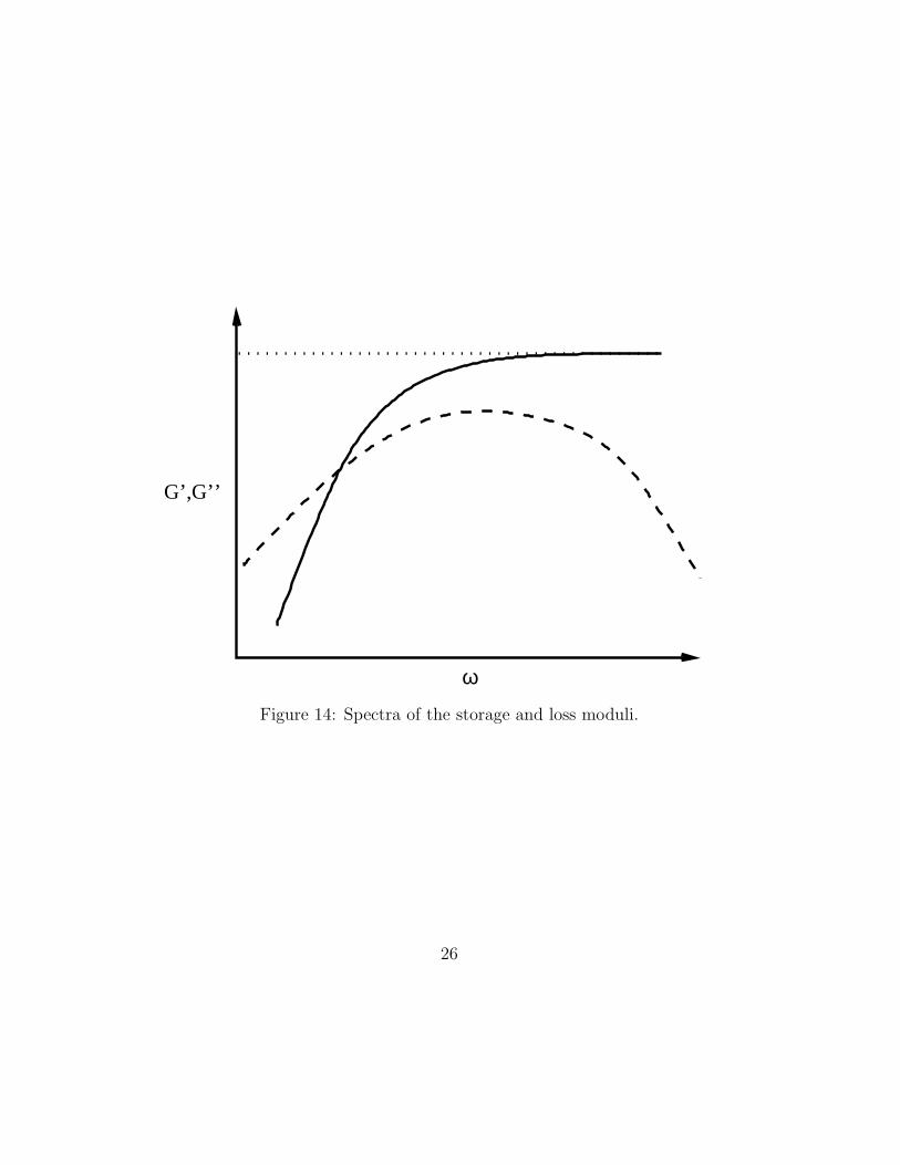
The shapes of the storage and loss moduli ‘spectra’ are shown as a function offrequency in figure 14. The storage modulus decreases proportional to ω2 inthe limit of low frequency, and attains a constant value at high frequency. Theloss modulus decreases proportional to ω at low frequency, and proportionalto ω−1 at high frequency. A parameter often quoted in literature is the ‘losstangent’ tan δ, which is defined as

tan δ = (G′′/G′) (32)

This provides the ratio of viscous to elastic response. This goes to infinityproportional to (1/ω) at low frequency, indicating that the response is pri-marily viscous at low frequency. At high frequency this goes to zero as (1/ω)indicating that the response is dominated by elasticity at high frequency.

The above formalism can easily be extended to the generalised Maxwellmodel, for example. The storage and loss moduli in this case are related tothe time constants and viscosities of the individual Maxwell elements.

G′ =n∑

i=1

Giτ2i ω2

1 + ω2τ 2i

G′′ =n∑

i=1

ηiω

1 + ω2τ 2i

(33)

where Gi, ηi and τi are the parameters in the equations for the individualMaxwell elements.

The shape of the storage and loss modulus curves is useful for deducingquantitative information about the relaxation times in the substance. Forexample, the loss modulus G′′ has a peak when ω = (1/τ) for a Maxwellfluid with a single time constant. For a generalised Maxwell fluid with twoelements, for example, there are two peaks at ω = (1/τ1) and (1/τ2) in theloss modulus spectrum. This implies that there are two rheological relaxationmechanisms in the system, and provides their time constants. This could beused to deduce the structure of these fluids. We will examine this a littlefurther while dealing with specific fluids.

25

G’,G’’

ω

Figure 14: Spectra of the storage and loss moduli.

26

4 Kinematics

This is the subject of the description of motion, without reference to theforces that cause this motion. Here, we assume that time and space arecontinuous, and identify a set of particles by specifying their location at atime (xo, t0). As the particles move, we follow their positions as a functionof time {x, t}. These positions are determined by solving the equations ofmotion for the particles, which we have not yet derived. Thus, the positionsof the particles at time t can be written as:

x(t) = x(xo, t) (34)

Note that x and t are independent variables; we can find the location of theparticle only if the initial location xo is given. Further, we can also expressthe (initial) position of the particles at time t0 as a function of their (final)positions at t:

xo(t0) = xo(x, t0) (35)

4.1 Lagrangian and Eulerian descriptions

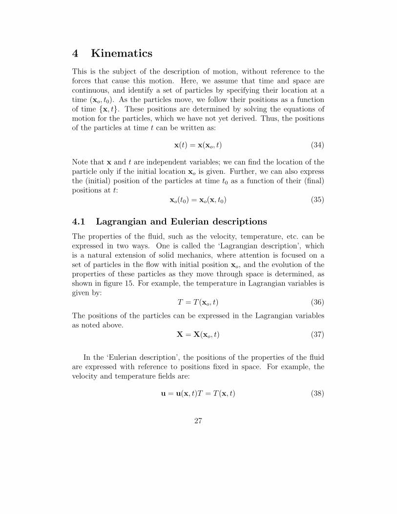
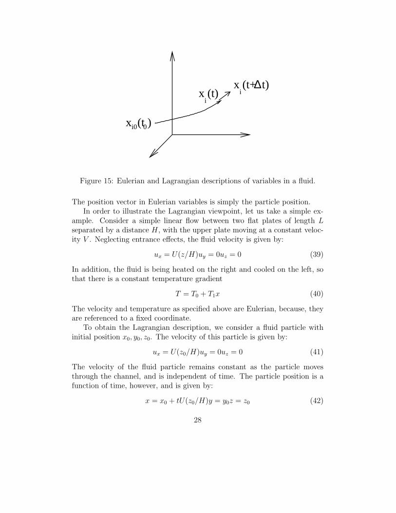
The properties of the fluid, such as the velocity, temperature, etc. can beexpressed in two ways. One is called the ‘Lagrangian description’, whichis a natural extension of solid mechanics, where attention is focused on aset of particles in the flow with initial position xo, and the evolution of theproperties of these particles as they move through space is determined, asshown in figure 15. For example, the temperature in Lagrangian variables isgiven by:

T = T (xo, t) (36)

The positions of the particles can be expressed in the Lagrangian variablesas noted above.

X = X(xo, t) (37)

In the ‘Eulerian description’, the positions of the properties of the fluidare expressed with reference to positions fixed in space. For example, thevelocity and temperature fields are:

u = u(x, t)T = T (x, t) (38)

27

x (t )i0 0

x (t)i

x (t+ t)i

∆

Figure 15: Eulerian and Lagrangian descriptions of variables in a fluid.

The position vector in Eulerian variables is simply the particle position.In order to illustrate the Lagrangian viewpoint, let us take a simple ex-

ample. Consider a simple linear flow between two flat plates of length Lseparated by a distance H , with the upper plate moving at a constant veloc-ity V . Neglecting entrance effects, the fluid velocity is given by:

ux = U(z/H)uy = 0uz = 0 (39)

In addition, the fluid is being heated on the right and cooled on the left, sothat there is a constant temperature gradient

T = T0 + T1x (40)

The velocity and temperature as specified above are Eulerian, because, theyare referenced to a fixed coordinate.

To obtain the Lagrangian description, we consider a fluid particle withinitial position x0, y0, z0. The velocity of this particle is given by:

ux = U(z0/H)uy = 0uz = 0 (41)

The velocity of the fluid particle remains constant as the particle movesthrough the channel, and is independent of time. The particle position is afunction of time, however, and is given by:

x = x0 + tU(z0/H)y = y0z = z0 (42)

28

From the equation for the temperature profile along the length of the channel,we can obtain the Lagrangian form of the temperature profile as well:

T = T0 + T1x = T0 + T1[x0 + tU(z0/H)] (43)

This gives the Lagrangian form of the particle position, velocity and temper-ature for the simple flow that we have considered. For more complex flows, itis very difficult to obtain the Lagrangian description of the particle motion,and this description is not often used.

4.2 Substantial derivatives

Next, we come to the subject of the time derivatives of the properties of afluid flow. In the Eulerian description, we focus only on the properties asa function of the positions in space. However, note that the position of thefluid particles are themselves a function of time, and it is often necessary todetermine the rate of the change of the properties of a given particle as afunction of time, as shown in figure 15. This derivative is referred to as theLagrangian derivative or the substantial derivative:

DA

Dt= {dA

dt}|

xo(44)

where A is any general property, and we have explicitly written the subscriptto note that the derivative is taken in the Lagrangian viewpoint, following theparticle positions in space. For example, consider the substantial derivativeof the temperature of a particle as it moves along the flow over a time interval∆t:

DT

Dt= lim

∆t→0

[

T (x + ∆x, t + ∆t) − T (x, t)

∆t

]

= lim∆t→0

[

T (x + u∆t, t + ∆t) − T (x, t)

∆t

]

(45)

Taking the limit ∆t → 0, and using chain rule for differentiation, we obtain,

DT

dt=

∂T

∂t+ ux

∂T

∂x+ uy

∂T

∂y+ uz

∂T

∂z

=∂T

∂t+ u.∇T (46)

29

where

∇ = ex∂

∂x+ ey

∂

∂y+ ez

∂

∂z(47)

is the gradient operator. The relation between the Eulerian and Lagrangianderivative for the problem just considered can be easily derived. In thepresent example, the Eulerian derivative of the temperature field is zero,because the temperature field has attained steady state. The substantialderivative is given by:

DT

Dt= u.∇T = ux

∂T

∂x= (Uz/H)T1 (48)

This can also be obtained by directly taking the time derivative of the tem-perature field in the Lagrangian description.

4.3 Decomposition of the strain rate tensor

The ‘strain rate’ tensor refers to the relative motion of the fluid particles inthe flow. For example, consider a differential volume dV , and a two particleslocated at x and x + ∆x in the volume, separated by a short distance ∆x.The velocity of the two particles are u and u + ∆u. The relative velocity ofthe particles can be expressed in tensor calculus as:

du = (∇u).∆x (49)

where ∇u is the gradient of the velocity which is a second order tensor. Inmatrix notation, this can be expressed as:

dux

duy

duz

=

∂ux

∂x∂ux

∂y∂ux

∂z∂uy

∂x∂uy

∂y∂uy

∂z∂uz

∂x∂uz

∂y∂uz

∂z

dxdydz

(50)

The second order tensor, ∇u, can be separated into two components, a sym-metric and an antisymmetric component, S + A, which are given by:

S =1

2(∇u + (∇u)T ) (51)

A =1

2(∇u − (∇u)T ) (52)

30

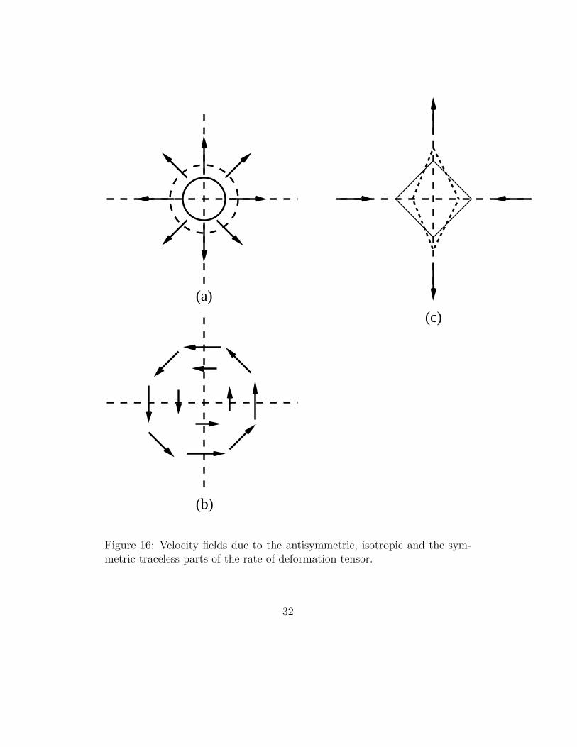
The antisymmetric part of the strain rate tensor represents rotationalflow. Consider a two dimensional flow field in which the rate of deformationtensor is antisymmetric,

(

∆ux

∆uy

)

=

(

0 −aa 0

)(

∆x∆y

)

(53)

The flow relative to the origin due to this rate of deformation tensor is shownin figure 16(a). It is clearly seen that the resulting flow is rotational, andthe angular velocity at a displacement ∆r from the origin is a∆r in theanticlockwise direction.

∆u =1

2∆x × ω (54)

where × is the cross product, and the vorticity ω is,

ω = ∇× u (55)

The symmetric part of the stress tensor can be further separated into twocomponents as follows:

S = E +I

3(Sxx + Syy + Szz) (56)

where S is the symmetric traceless part of the strain tensor, I is the identitytensor,

I =

1 0 00 1 00 0 1

(57)

and (1/3)I(Sxx + Syy + Szz) is the isotropic part. ‘Traceless’ implies thatthe trace of the tensor, which is Exx + Eyy + Ezz, is zero. The symmetrictraceless part, E, is called the ‘extensional strain’, while the isotropic part,(1/3)I(Sxx+Syy +Szz), corresponds to radial motion. Note that the isotropicpart can also be written as,

I

3(Sxx + Syy + Szz) =

I

3

(

∂ux

∂x+

∂uy

∂y+

∂uz

∂z

)

=I

3∇.u (58)

31

(b)

(a)

(c)

Figure 16: Velocity fields due to the antisymmetric, isotropic and the sym-metric traceless parts of the rate of deformation tensor.

32

Thus, the isotropic part of the rate of deformation tensor is related to thedivergence of the velocity.

The velocity difference between the two neighbouring points due to theisotropic part of the rate of deformation tensor is given by

(

∆ux

∆uy

)

=

(

s 00 s

)(

∆x∆y

)

(59)

The above equation implies that the relative velocity between two points dueto the isotropic component is directed along their line of separation, and thisrepresents a radial motion, as shown in figure 16(b). The radial motion isoutward if s is positive, and inward if s is negative.

The symmetric traceless part represents an ‘extensional strain’, in whichthere is no change in density and no solid body rotation. In two dimensions,the simplest example of the velocity field due to a symmetric traceless rateof deformation tensor is

(

∆ux

∆uy

)

=

(

s 00 −s

)(

∆x∆y

)

(60)

The relative velocity of points near the origin due to this rate of deformationtensor is shown in figure 16(c). It is found that the fluid element near theorigin deforms in such a way that there is no rotation of the principle axes,and there is no change in the total volume. This type of deformation iscalled ‘pure extensional strain’ and is responsible for the internal stresses inthe fluid.

The symmetric traceless part of the rate of deformation tensor also con-tains information about the extensional and compressional axes of the flow.A symmetric tensor of order n × n has n eigenvalues which are real, and neigenvectors which are orthogonal. The sum of the eigenvalues of the tensoris equal to the sum of the diagonal elements. Therefore, for the symmetrictraceless rate of deformation tensor, the sum of the eigenvalues is equal tozero. This means that, in two dimensions, the two eigenvectors are equal inmagnitude and opposite in sign. In three dimensions, the sum of the eigen-values of the tensor is equal to zero. If Ev is the column of the normalisedeigenvectors of the symmetric traceless tensor E,

Ev =

ev1

ev2

ev3

(61)

33

and if the eigenvalues are λ1, λ2 and λ3, then the tensor can be written as,

E−1v EEv =

λ1 0 00 λ2 00 0 λ3

(62)

Also, the eigenvectors satisfy the equation E−1v = ET

v .Equation 62 can be interpreted as follows. The difference in velocity

between two neighbouring locations due to a the deviatoric part of the rateof deformation tensor is,

∆ux

∆uy

∆uz

= E

∆x∆y∆z

(63)

This can be rewritten, using equation 62, as,

∆ux

∆uy

∆uz

= Ev

λ1 0 00 λ2 00 0 λ3

E−1v

∆x∆y∆z

(64)

If we define a new co-ordinate system,

∆x′

∆y′

∆z′

= E−1v

∆x∆y∆z

(65)

and velocity

∆u′

x

∆u′

y

∆u′

z

= E−1v

∆ux

∆uy

∆uz

(66)

Then the equation for the velocity difference between two neighbouring lo-cations becomes,

∆u′

x

∆u′

y

∆u′

z

=

λ1 0 00 λ2 00 0 λ3

∆x′

∆y′

∆z′

(67)

The operations in 65 and 66 are just equivalent to rotating the co-ordinatesystem. Equation 67 indicates that in this rotated co-ordinate system, the

34

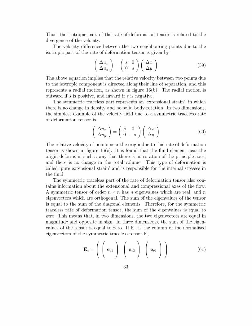
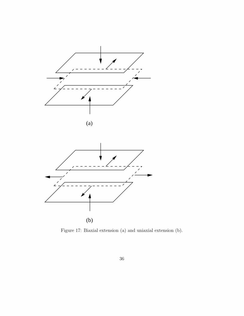
difference in velocity are directed along the axes of the rotated co-ordinatesystem. Since the sum of the three eigenvalues are zero, there are threepossibilities for the signs of the three eigenvalues. If two of the eigenvaluesare positive and one is negative, then there is extension along two axes andcompression along one axis, as shown in figure 17(a). This is called bi-axial extension. If one of the eigenvalues is positive and the other two arenegative, then there is compression along two axes and extension along oneaxis, as shown in figure 17(b). This is called uniaxial extension. If one of theeigenvalue is zero, then there is extension along one axis, compression alongthe second and no deformation along the third axis. This is called planeextension, as shown in figure 16(c)

5 Conservation of mass

The mass conservation equation simply states that mass cannot be createdor destroyed. Therefore, for any volume of fluid,

(

Rate of massaccumulation

)

=

(

Rate of massIN

)

−(

Rate of massOUT

)

(68)

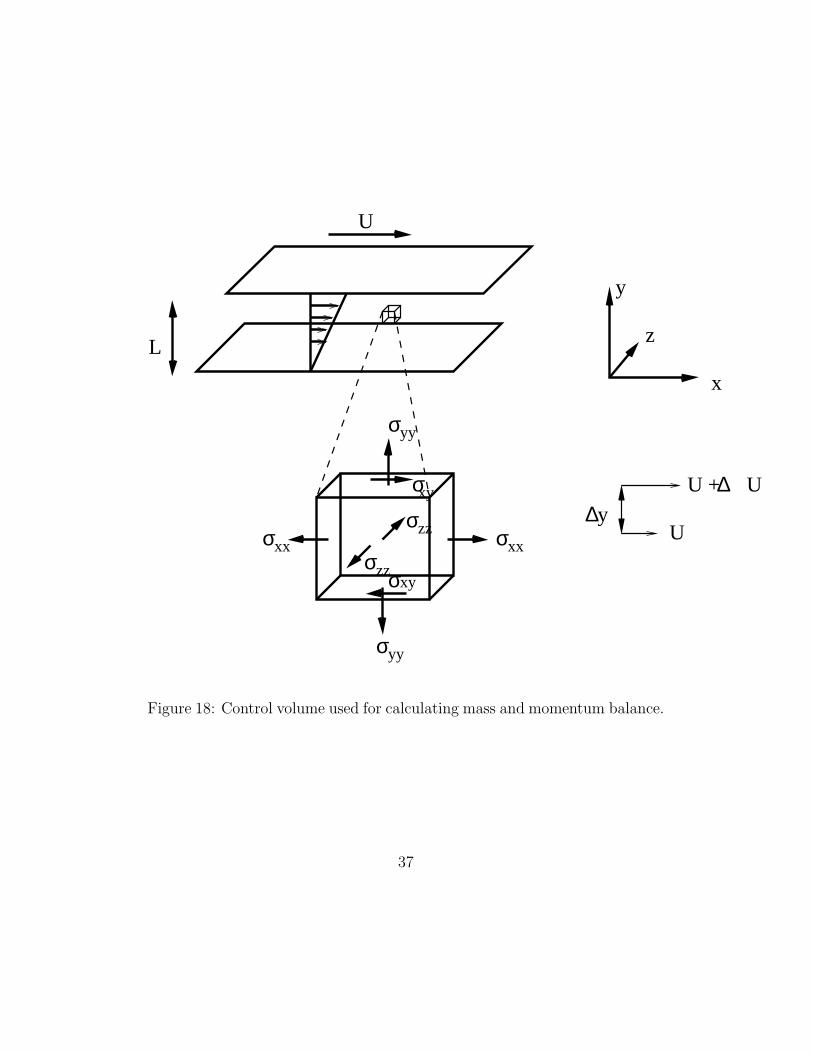
Consider the volume of fluid shown in figure 18. This volume has a totalvolume ∆x∆y∆z, and it has six faces. The rate of mass in through the face atx is (ρux)|x ∆y∆z, while the rate of mass out at x+∆x is (ρux)|x+∆x ∆y∆z.Similar expressions can be written for the rates of mass flow through the otherfour faces. The total increase in mass for this volume is (∂ρ/∂t)∆x∆y∆z.Therefore, the mass conservation equation states that

∆x∆y∆z∂ρ

∂t= ∆y∆z[ (ρux)|x − (ρux)|x+∆x]

+∆x∆z[ (ρuy)|y − (ρuy)|y+∆y]

= ∆x∆y[ (ρuz)|z − (ρuz)|z+∆z] (69)

Dividing by ∆x∆y∆z, and taking the limit as these approach zero, we get

∂ρ

∂t= −

(

∂(ρux)

∂x+

∂(ρuy)

∂y+

∂(ρuz)

∂z

)

(70)

35

(a)

(b)

Figure 17: Biaxial extension (a) and uniaxial extension (b).

36

x

y

z

U

L

σσ

σ

σ

xxxx

yy

yy

σzz

σzz

σ

σ

xy

xy

U

U + U∆∆y

Figure 18: Control volume used for calculating mass and momentum balance.

37

The above equation can often be written using the substantial derivative

∂ρ

∂t+

(

ux∂ρ

∂x+ uy

∂ρ

∂y+ uz

∂ρ

∂z

)

= −ρ

(

∂ux

∂x+

∂uy

∂y+

∂uz

∂z

)

(71)

The left side of the above equation is the substantial derivative, while theright side can be written as

Dρ

Dt= −ρ(∇.u) (72)

The above equation describes the change in density for a material element offluid which is moving along with the mean flow. A special case is when thedensity does not change, so that (Dρ/Dt) is identically zero. In this case,the continuity equation reduces to

∂ux

∂x+

∂uy

∂y+

∂uz

∂z= 0 (73)

This is just the isotropic part of the rate of deformation tensor, which corre-sponds to volumetric compression or expansion. Therefore, if this is zero, itimplies that there is no volumetric expansion or compression, and if mass isconserved then the density has to be a constant. Fluids which obey this con-dition are called ‘incompressible’ fluids. Most fluids that we use in practicalapplications are incompressible fluids; in fact all liquids can be consideredincompressible for practical purposes. Compressibility effects only becomeimportant in gases when the speed of the gas approaches the speed of sound,332 m/s.

6 Momentum conservation

The momentum conservation equation is a consequence of Newton’s secondlaw of motion, which states that the rate of change of momentum in a dif-ferential volume is equal to the total force acting on it. The momentum in avolume V (t) is given by:

P =∫

V (t)dV ρu (74)

and Newton’s second law states that the rate of change of momentum in amoving differential volume is equal to the sum of the applied forces,

DPi

Dt=

d

dt

∫

V (t)dV (ρu) = Sum of forces (75)

38

Here, note that the momentum conservation equation is written for a movingfluid element. In a manner similar to the mass conservation equation, theintegral over a moving fluid element can be written in a Eulerian referenceframe as,

∫

V (t)dV

(

∂ρu

∂t+ ∇.(ρuu)

)

= Sum of forces (76)

The forces acting on a fluid are usually of two types. The first is the bodyforce, which act on the bulk of the fluid, such as the force of gravity, andthe surface forces, which act at the surface of the control volume. If F is thebody force per unit mass of the fluid, and R is the force per unit area actingat the surface, then the momentum conservation equation can be written as:

∫

V (t)dV

(

∂(ρu)

∂t+ ∇.(ρuu)

)

=∫

V (t)dV F +

∫

SdSR (77)

where S is the surface of the volume V (t).In order to complete the derivation of the equations of motion, it is nec-

essary to specify the form of the body and surface forces. The form of thebody forces is well known – the force due to gravity per unit mass is just thegravitational acceleration g, while the force due to centrifugal acceleration isgiven by ωR2 where ω is the angular velocity and R is the radius. The formof the surface force is not specified a-priori, however, and the ‘constitutiveequations’ are required to relate the surface forces to the motion of the fluid.But before specifying the nature of the surface forces, one can derive someof the properties of the forces using symmetry considerations.

The force acting on a surface will, in general, depend on the orientationof the surface, and will be a function of the unit normal to the surface, inaddition to the other fluid properties:

R = R(n) (78)

We can use symmetry considerations to show that the force is a linear func-tion of the unit normal to the surface. If we consider a surface dividing thefluid at a point P , then the force acting on the two sides of the surface haveto be equal according to Newton’s third law. Since the unit normal to thetwo sides are just the negative of each other, this implies that:

R(−n) = −R(n) (79)

39

This suggests that the surface force could be a linear function of the normal:

R = T.n (80)

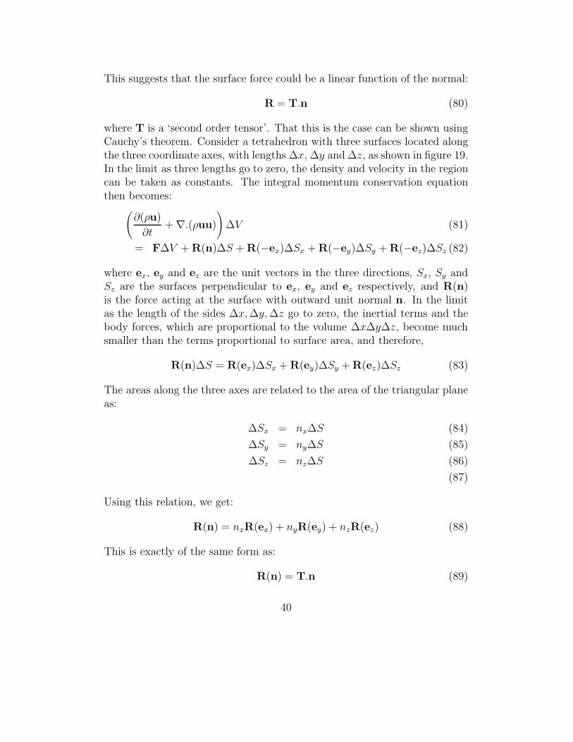
where T is a ‘second order tensor’. That this is the case can be shown usingCauchy’s theorem. Consider a tetrahedron with three surfaces located alongthe three coordinate axes, with lengths ∆x, ∆y and ∆z, as shown in figure 19.In the limit as three lengths go to zero, the density and velocity in the regioncan be taken as constants. The integral momentum conservation equationthen becomes:

(

∂(ρu)

∂t+ ∇.(ρuu)

)

∆V (81)

= F∆V + R(n)∆S + R(−ex)∆Sx + R(−ey)∆Sy + R(−ez)∆Sz (82)

where ex, ey and ez are the unit vectors in the three directions, Sx, Sy andSz are the surfaces perpendicular to ex, ey and ez respectively, and R(n)is the force acting at the surface with outward unit normal n. In the limitas the length of the sides ∆x, ∆y, ∆z go to zero, the inertial terms and thebody forces, which are proportional to the volume ∆x∆y∆z, become muchsmaller than the terms proportional to surface area, and therefore,

R(n)∆S = R(ex)∆Sx + R(ey)∆Sy + R(ez)∆Sz (83)

The areas along the three axes are related to the area of the triangular planeas:

∆Sx = nx∆S (84)

∆Sy = ny∆S (85)

∆Sz = nz∆S (86)

(87)

Using this relation, we get:

R(n) = nxR(ex) + nyR(ey) + nzR(ez) (88)

This is exactly of the same form as:

R(n) = T.n (89)

40

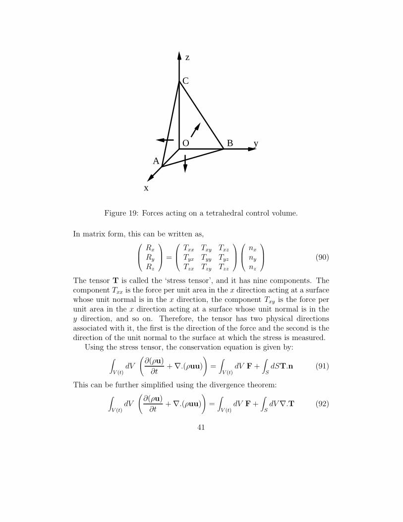
x

BO

A

C

y

z

Figure 19: Forces acting on a tetrahedral control volume.

In matrix form, this can be written as,

Rx

Ry

Rz

=

Txx Txy Txz

Tyx Tyy Tyz

Tzx Tzy Tzz

nx

ny

nz

(90)

The tensor T is called the ‘stress tensor’, and it has nine components. Thecomponent Txx is the force per unit area in the x direction acting at a surfacewhose unit normal is in the x direction, the component Txy is the force perunit area in the x direction acting at a surface whose unit normal is in they direction, and so on. Therefore, the tensor has two physical directionsassociated with it, the first is the direction of the force and the second is thedirection of the unit normal to the surface at which the stress is measured.

Using the stress tensor, the conservation equation is given by:∫

V (t)dV

(

∂(ρu)

∂t+ ∇.(ρuu)

)

=∫

V (t)dV F +

∫

SdST.n (91)

This can be further simplified using the divergence theorem:∫

V (t)dV

(

∂(ρu)

∂t+ ∇.(ρuu)

)

=∫

V (t)dV F +

∫

SdV ∇.T (92)

41

Since the above equation is valid for any differential volume in the fluid, theintegrand must be equal to zero:

(

∂(ρu)

∂t+ ∇.(ρuu)

)

= F + ∇.T (93)

The above equation can be simplified using the mass conservation equation:

ρ

(

∂u

∂t+ u∇.u

)

= F + ∇.T (94)

A additional property of the stress tensor, which is obtained from theangular momentum equation, is that the stress tensor is symmetric. That is,Txy = Tyx, Txz = Tzx and Tyz = Tzy in equation 90.

7 Constitutive equations for the stress tensor

Just as we had earlier separated the strain rate tensor into an antisymmetrictraceless part, a symmetric part and an isotropic part, it is conventional toseparate the stress tensor into an isotropic part and a symmetric traceless‘deviatoric’ part:

T = −pI + σ (95)

where p is the pressure in the isotropic pressure in the fluid, p = −(1/3)(Txx+Tyy +Tzz), and σ is the second order ‘deviatoric’ stress tensor which is trace-less, (σxx + σyy + σzz) = 0. In the absence of fluid flow, the deviatoric partof the stress tensor σ becomes zero, and pressure field is related to the localdensity of the system by a thermodynamic equation of state.

The shear stress, σ, is a function of the fluid velocity. However, thestress cannot depend on the fluid velocity itself, because the stress has tobe invariant under a ‘Galilean transformation’, i.e., when the velocity of theentire system is changed by a constant value. Therefore, the stress has todepend on the gradient of the fluid velocity. In a ‘Newtonian fluid’, we makethe assumption that the stress is a linear function of the velocity gradient.In general, the linear relation can be written as:

σ = η.∇u (96)

where η is a fourth order tensor. This tensor is a property of the fluid. Inan isotropic fluid, there is no preferred direction in space, and therefore, the

42

tensor η should be independent of direction. In this case, it can be shownthat the relationship between the stress and strain rate is of the form,

σ = η(∇u + (∇u)T − (2/3)I∇.u) (97)

where η is the ‘coefficient of viscosity’ of the fluid. This can also be expressedin terms of the rate of strain tensor:

σ = 2ηE (98)

where E is the symmetric traceless part of the rate of deformation tensor.The above constitutive equation was derived for a Newtonian fluid with

the assumption that the shear stress is a linear function of the strain rate.However, the stress could be a non-linear function of the strain rate in com-plex fluids such as polymers solutions.

σ = f(E) (99)

Since eij is a frame indifferent tensor, any tensor that can be written as:

σ = scalar ×E (100)

satisfies the conditions of frame indifference. There are three frame indifferentscalars that can be constructed from the tensor ∇u:

I1 = ∇.u I2 = E:E I3 = Det(E) (101)

Therefore, any constitutive relation can be written of the form,

σ = η(I1, I2, I3)E (102)

would satisfy the requirements of material frame indifference. Of these frame-indifferent scalars, I1 = 0 for an incompressible fluid.

The constitutive equation for the stress tensor can be inserted into themomentum conservation equation to obtain:

∂tρ + ∂i(ρvi) = 0ρ∂tvi + ρvj∂jvi = −∂ip + eta (∂2

j vi − (2/3)∂i∂jvj)(103)

These are the Navier - Stokes mass and momentum conservation equations.For an incompressible fluid, where the density is a constant in both spaceand time, the Navier - Stokes equations have a particularly simple form:

∂ivi = 0∂tvi + vj∂jvi = −ρ−1∂ip + ν∂2

j vi(104)

where ν = (η/ρ) is the kinematic viscosity.

43

Figure 20: A polymer molecule (left) and the bead-spring representation ofthe polymer molecule (right).

8 Polymer conformation:

The most widely studied non-Newtonian fluids are polymer solutions andpolymer melts. A polymer is a molecule with high molecular weight obtainedby covalently bonding a large number of units or monomers, so that thelinear length of the molecular is large compared to the molecular diameter.Polymers can be thought of as long flexible strings, and have many interestingproperties because of their linear nature. In solutions and in melts, they arein a highly coiled state, as shown in figure 20. In solutions and melts, thesesprings are in a highly coiled state.

A useful physical picture is obtained if we consider these strings as un-dergoing a random walk. The random walk proceeds in steps of equal length,called the ‘Kuhn segment length’ (which is a few times larger than themonomer size), with a random change in direction after each step. The aver-age end-to-end distance of a random walk with N steps increases proportionalto

√N . Therefore, one would expect the linear size of a polymer molecule

to increase proportional to N1/2, where N is the number of monomers, ifthe molecule is accurately described by a random walk. However, in realsolutions, there is an additional factor which comes into play, which is thatthe polymer molecule cannot cross itself. Due to this, the radius of gyrationof a polymer molecule actually increases with a slightly higher power, N0.58.

If we assume a simple random walk model, then the average end-to-end distance of a polymer molecule increases proportional to N1/2, where

44

N is the number of Kuhn segments. The probability of finding a configura-tion with a particular end-to-end distance can be evaluated from entropicarguments, based on the number of configurations corresponding to thisend-to-end distance. Based on simple arguments for a Gaussian chain, itcan be inferred the probability that the end-to-end distance is x is propor-tional to exp (−x2/(Nl2)), where l is the Kuhn segment length and N is thenumber of Kuhn segments. This is equivalent to a probability of the formexp (−Ex/kT ), where the energy Ex for a molecule with end-to-end distancex is Ex = (kT/Nl2)x2. If we consider the factor (2kT/Nl2) as a spring con-stant kn, then the energy penalty is of the form Ex = (knx

2/2). This is justthe stretching energy of a spring with spring-constant kn. This leads to astill simpler bead-spring representation of a molecule, which is a linear springbetween two beads which has a spring constant kn, as shown in figure 8.

In the bead-spring model, the stress due to the polymers is expressed interms of the second order conformation tensor, has a very simple form,

Tp = cpknxx = cpknQ (105)

where the term on the right contains the tensor product of the end-to-enddisplacement vector x, and cp is the polymer concentration. The tensorQ = xx is referred to as the ‘polymer conformation tensor’ which basicallyprovides information about the state of stretch of the polymers. Here, wehave a situation where the local flow field affects the polymers by stretchingand rotating them, and the state of stretch of the polymers provides an addi-tional component of the stress which in turn affects the flow field. Therefore,in a fluid-dynamical description, it is necessary to have coupled equations forboth the flow field as well as the conformation tensor of the polymers.

In the equation for the conformation tensor of the polymer, there areterms corresponding to the stretching and bending of the polymers due tothe imposed flow, and there is a ‘spring’ force which tends to reduce thepolymer conformation back to its equilibrium state. From the Gaussianapproximation for the polymer end-to-end distance, the conformation tensorQeq at equilibrium is an isotropic tensor with no preferred direction,

Qeq =kT

knI (106)

The simplest equation for the conformation tensor states the polymer tendsto relax back to its equilibrium conformation with a time constant,

DQ

Dt= −Q −Qeq

τ(107)

45

There are two new terms introduced above, the relaxation time τ and the‘upper convected’ derivative (D/Dt)on the left. First, the upper convectedderivative is defined as,

DQ

Dt=

∂Q

∂t+ u.∇Q − Q.∇u − (∇u)T .Q (108)

The first two terms on the right side are just the substantial derivative, butthe ‘upper convected’ derivative contains two additional terms. In our earlierdiscussion, we noted that the substantial derivative is a derivative in a refer-ence frame moving with the local fluid mean velocity. In a similar manner,the ‘upper convected’ derivative also contains terms due to the local rotationof fluid elements at a point. Since the rotation of the fluid elements willtend to rotate any bead-spring dumbbells immersed in the fluid, this rota-tion is included in the substantial derivative. Therefore, the upper-convectedderivative is a derivative in a reference frame moving and rotating with thelocal fluid element. On the right side of equation 108, the time constantτ = (ξ/kn) is the ratio of the spring constant and a ‘friction coefficient’ ξ,which represents the force exerted on the beads due to the fluid flow pastthe beads. If the fluid is flowing with a velocity v past the beads, the forceexerted can be written as F = −ξv in the linear approximation. The ratioof this frictional force and the spring constant is the time constant.

Once the value of Q is known, then equation 105 can be used to evaluatethe polymer stress, which is then inserted into the momentum conservationequation of the fluid,

ρ

(

∂u

∂t+ u.∇u

)

= −∇p + η∇2u + ∇.Tp (109)

The polymer stress is usually written in an alternate, but completely equiv-alent, form to equation 105,

Tp =ηpkn

τkT(Q −Qeq) (110)

where ηp = (cpkTτ) is the polymer viscosity, and the only difference be-tween the above equation and equation 105 is that we have removed theisotropic part proportional to Qeq. Equations 109 and 110 constitute theupper-convected Maxwell model for a polymeric fluid.

46