Fundamentals of the Finite Element Method for Heat and Mass TransferSecond Edition

P. Nithiarasu, R. W. Lewis, and K. N. Seetharamu

Fundamentals of the Finite ElementMethod for Heat and Mass Transfer

WILEY SERIES IN COMPUTATIONAL MECHANICS

Series Advisors:

Rene de BorstPerumal NithiarasuTayfun E. TezduyarGenki YagawaTarek Zohdi

Fundamentals of the Finite Element Nithiarasu, Lewis January 2016Method for Heat and Mass Transfer and Seetharamu

Introduction to Computational Contact Konyukhov April 2015Mechanics: A Geometrical Approach

Extended Finite Element Method: Khoei December 2014Theory and Applications

Computational Fluid-Structure Bazilevs, Takizawa and January 2013Interaction: Methods and Applications Tezduyar

Introduction to Finite Strain Theory for Hashiguchi and Yamakawa November 2012Continuum Elasto-Plasticity

Nonlinear Finite Element Analysis of De Borst, Crisfield, Remmers August 2012Solids and Structures, Second Edition and Verhoosel

An Introduction to Mathematical Oden November 2011Modeling: A Course in Mechanics

Computational Mechanics of Munjiza, Knight and Rougier November 2011Discontinua

Introduction to Finite Element Analysis: Szabo and Babuska March 2011Formulation, Verification and Validation

Fundamentals of the Finite ElementMethod for Heat and Mass Transfer

Second Edition

P. NithiarasuZienkiewicz Centre for Computational EngineeringCollege of Engineering, Swansea University, UK

R. W. LewisZienkiewicz Centre for Computational EngineeringCollege of Engineering, Swansea University, UK

K. N. SeetharamuDepartment of Mechanical Engineering

PESIT, Bangalore, Karnataka, India

This edition first published 2016 © 2016 by John Wiley & Sons, Ltd.First edition published 2004 © 2004 by John Wiley & Sons, Ltd.

Registered officeJohn Wiley & Sons Ltd, The Atrium, Southern Gate, Chichester, West Sussex, PO19 8SQ, United Kingdom

For details of our global editorial offices, for customer services and for information about how to apply forpermission to reuse the copyright material in this book please see our website at www.wiley.com.

The right of the author to be identified as the author of this work has been asserted in accordance with the Copyright,Designs and Patents Act 1988.

All rights reserved. No part of this publication may be reproduced, stored in a retrieval system, or transmitted, in anyform or by any means, electronic, mechanical, photocopying, recording or otherwise, except as permitted by the UKCopyright, Designs and Patents Act 1988, without the prior permission of the publisher.

Wiley also publishes its books in a variety of electronic formats. Some content that appears in print may not beavailable in electronic books.

Designations used by companies to distinguish their products are often claimed as trademarks. All brand names andproduct names used in this book are trade names, service marks, trademarks or registered trademarks of theirrespective owners. The publisher is not associated with any product or vendor mentioned in this book.

Limit of Liability/Disclaimer of Warranty: While the publisher and author have used their best efforts in preparingthis book, they make no representations or warranties with respect to the accuracy or completeness of the contents ofthis book and specifically disclaim any implied warranties of merchantability or fitness for a particular purpose. It issold on the understanding that the publisher is not engaged in rendering professional services and neither thepublisher nor the author shall be liable for damages arising herefrom. If professional advice or other expertassistance is required, the services of a competent professional should be sought.

The advice and strategies contained herein may not be suitable for every situation. In view of ongoing research,equipment modifications, changes in governmental regulations, and the constant flow of information relating to theuse of experimental reagents, equipment, and devices, the reader is urged to review and evaluate the informationprovided in the package insert or instructions for each chemical, piece of equipment, reagent, or device for, amongother things, any changes in the instructions or indication of usage and for added warnings and precautions. The factthat an organization or Website is referred to in this work as a citation and/or a potential source of furtherinformation does not mean that the author or the publisher endorses the information the organization or Website mayprovide or recommendations it may make. Further, readers should be aware that Internet Websites listed in this workmay have changed or disappeared between when this work was written and when it is read. No warranty may becreated or extended by any promotional statements for this work. Neither the publisher nor the author shall be liablefor any damages arising herefrom.

Library of Congress Cataloging-in-Publication Data

Names: Nithiarasu, Perumal. | Lewis, R. W. (Roland Wynne) | Seetharamu, K. N.| Lewis, R. W. (Roland Wynne). Fundamentals of the finite element method for heat and fluid flow.

Title: Fundamentals of the finite element method for heat and mass transfer.Description: Second edition / P. Nithiarasu, R.W. Lewis, K.N. Seetharamu. | Chichester, West Sussex :

John Wiley & Sons, Inc., 2016. | First edition: Fundamentals of the finite element method for heat and fluid flow /Roland W. Lewis, Perumal Nithiarasu, Kankanhalli N. Seetharamu (Hoboken, NJ : Wiley, 2004). | Includesbibliographical references and index.

Identifiers: LCCN 2015034600 | ISBN 9780470756256 (cloth : alk. paper)Subjects: LCSH: Finite element method. | Heat equation. | Heat–Transmission.

| Fluid dynamics. | Mass transfer.Classification: LCC QC20.7.F56 L49 2016 | DDC 530.15/5353–dc23 LC record available athttp://lccn.loc.gov/2015034600

A catalogue record for this book is available from the British Library.

Set in 10/12.5pt Times by Aptara Inc., New Delhi, India.

Cover images: courtesy of the authors.

1 2016

Contents

Preface to the Second Edition xii

Series Editor’s Preface xiv

1 Introduction 11.1 Importance of Heat and Mass Transfer . . . . . . . . . . . . . . . . . . . . . . . . . . . . . . . . . . 11.2 Heat Transfer Modes . . . . . . . . . . . . . . . . . . . . . . . . . . . . . . . . . . . . . . . . . . . . . . . . . . 21.3 The Laws of Heat Transfer . . . . . . . . . . . . . . . . . . . . . . . . . . . . . . . . . . . . . . . . . . . . 31.4 Mathematical Formulation of Some Heat Transfer Problems . . . . . . . . . . . . . . 5

1.4.1 Heat Transfer from a Plate Exposed to Solar Heat Flux . . . . . . . . . . . 51.4.2 Incandescent Lamp . . . . . . . . . . . . . . . . . . . . . . . . . . . . . . . . . . . . . . . . . . . 71.4.3 Systems with a Relative Motion and Internal Heat Generation . . . . . 8

1.5 Heat Conduction Equation . . . . . . . . . . . . . . . . . . . . . . . . . . . . . . . . . . . . . . . . . . . . . 101.6 Mass Transfer . . . . . . . . . . . . . . . . . . . . . . . . . . . . . . . . . . . . . . . . . . . . . . . . . . . . . . . . 131.7 Boundary and Initial Conditions . . . . . . . . . . . . . . . . . . . . . . . . . . . . . . . . . . . . . . . . 131.8 Solution Methodology . . . . . . . . . . . . . . . . . . . . . . . . . . . . . . . . . . . . . . . . . . . . . . . . 151.9 Summary . . . . . . . . . . . . . . . . . . . . . . . . . . . . . . . . . . . . . . . . . . . . . . . . . . . . . . . . . . . . 151.10 Exercises . . . . . . . . . . . . . . . . . . . . . . . . . . . . . . . . . . . . . . . . . . . . . . . . . . . . . . . . . . . . 16References . . . . . . . . . . . . . . . . . . . . . . . . . . . . . . . . . . . . . . . . . . . . . . . . . . . . . . . . . . . . . . . . . 17

2 Some Basic Discrete Systems 192.1 Introduction . . . . . . . . . . . . . . . . . . . . . . . . . . . . . . . . . . . . . . . . . . . . . . . . . . . . . . . . . . 192.2 Steady-state Problems . . . . . . . . . . . . . . . . . . . . . . . . . . . . . . . . . . . . . . . . . . . . . . . . . 20

2.2.1 Heat Flow in a Composite Slab . . . . . . . . . . . . . . . . . . . . . . . . . . . . . . . . . 202.2.2 Fluid Flow Network . . . . . . . . . . . . . . . . . . . . . . . . . . . . . . . . . . . . . . . . . . 232.2.3 Heat Transfer in Heat Sinks . . . . . . . . . . . . . . . . . . . . . . . . . . . . . . . . . . . . 26

2.3 Transient Heat Transfer Problem . . . . . . . . . . . . . . . . . . . . . . . . . . . . . . . . . . . . . . . 282.4 Summary . . . . . . . . . . . . . . . . . . . . . . . . . . . . . . . . . . . . . . . . . . . . . . . . . . . . . . . . . . . . 312.5 Exercises . . . . . . . . . . . . . . . . . . . . . . . . . . . . . . . . . . . . . . . . . . . . . . . . . . . . . . . . . . . . 31References . . . . . . . . . . . . . . . . . . . . . . . . . . . . . . . . . . . . . . . . . . . . . . . . . . . . . . . . . . . . . . . . . 36

3 The Finite Element Method 393.1 Introduction . . . . . . . . . . . . . . . . . . . . . . . . . . . . . . . . . . . . . . . . . . . . . . . . . . . . . . . . . . 393.2 Elements and Shape Functions . . . . . . . . . . . . . . . . . . . . . . . . . . . . . . . . . . . . . . . . . 42

vi CONTENTS

3.2.1 One-dimensional Linear Element . . . . . . . . . . . . . . . . . . . . . . . . . . . . . . . 433.2.2 One-dimensional Quadratic Element . . . . . . . . . . . . . . . . . . . . . . . . . . . . 463.2.3 Two-dimensional Linear Triangular Element . . . . . . . . . . . . . . . . . . . . 493.2.4 Area Coordinates . . . . . . . . . . . . . . . . . . . . . . . . . . . . . . . . . . . . . . . . . . . . . 533.2.5 Quadratic Triangular Element . . . . . . . . . . . . . . . . . . . . . . . . . . . . . . . . . . 553.2.6 Two-dimensional Quadrilateral Elements . . . . . . . . . . . . . . . . . . . . . . . . 583.2.7 Isoparametric Elements . . . . . . . . . . . . . . . . . . . . . . . . . . . . . . . . . . . . . . . 633.2.8 Three-dimensional Elements . . . . . . . . . . . . . . . . . . . . . . . . . . . . . . . . . . . 72

3.3 Formulation (Element Characteristics) . . . . . . . . . . . . . . . . . . . . . . . . . . . . . . . . . . 763.3.1 Ritz Method (Heat Balance Integral Method – Goodman’s Method) 783.3.2 Rayleigh–Ritz Method (Variational Method) . . . . . . . . . . . . . . . . . . . . . 793.3.3 The Method of Weighted Residuals . . . . . . . . . . . . . . . . . . . . . . . . . . . . . 823.3.4 Galerkin Finite Element Method . . . . . . . . . . . . . . . . . . . . . . . . . . . . . . . 86

3.4 Formulation for the Heat Conduction Equation . . . . . . . . . . . . . . . . . . . . . . . . . . 893.4.1 Variational Approach . . . . . . . . . . . . . . . . . . . . . . . . . . . . . . . . . . . . . . . . . 903.4.2 The Galerkin Method . . . . . . . . . . . . . . . . . . . . . . . . . . . . . . . . . . . . . . . . . 93

3.5 Requirements for Interpolation Functions . . . . . . . . . . . . . . . . . . . . . . . . . . . . . . . 943.6 Summary . . . . . . . . . . . . . . . . . . . . . . . . . . . . . . . . . . . . . . . . . . . . . . . . . . . . . . . . . . . . 1003.7 Exercises . . . . . . . . . . . . . . . . . . . . . . . . . . . . . . . . . . . . . . . . . . . . . . . . . . . . . . . . . . . . 100References . . . . . . . . . . . . . . . . . . . . . . . . . . . . . . . . . . . . . . . . . . . . . . . . . . . . . . . . . . . . . . . . . 102

4 Steady-State Heat Conduction in One-dimension 1054.1 Introduction . . . . . . . . . . . . . . . . . . . . . . . . . . . . . . . . . . . . . . . . . . . . . . . . . . . . . . . . . . 1054.2 Plane Walls . . . . . . . . . . . . . . . . . . . . . . . . . . . . . . . . . . . . . . . . . . . . . . . . . . . . . . . . . . 105

4.2.1 Homogeneous Wall . . . . . . . . . . . . . . . . . . . . . . . . . . . . . . . . . . . . . . . . . . . 1054.2.2 Composite Wall . . . . . . . . . . . . . . . . . . . . . . . . . . . . . . . . . . . . . . . . . . . . . . 1074.2.3 Finite Element Discretization . . . . . . . . . . . . . . . . . . . . . . . . . . . . . . . . . . 1084.2.4 Wall with Varying Cross-sectional Area . . . . . . . . . . . . . . . . . . . . . . . . . 1104.2.5 Plane Wall with a Heat Source: Solution by Linear Elements . . . . . . 1124.2.6 Plane Wall with Heat Source: Solution by Quadratic Elements . . . . 1154.2.7 Plane Wall with a Heat Source: Solution by Modified Quadratic

Equations (Static Condensation) . . . . . . . . . . . . . . . . . . . . . . . . . . . . . . . . 1174.3 Radial Heat Conduction in a Cylinder Wall . . . . . . . . . . . . . . . . . . . . . . . . . . . . . . 1184.4 Solid Cylinder with Heat Source . . . . . . . . . . . . . . . . . . . . . . . . . . . . . . . . . . . . . . . 1204.5 Conduction – Convection Systems. . . . . . . . . . . . . . . . . . . . . . . . . . . . . . . . . . . . . . 1234.6 Summary . . . . . . . . . . . . . . . . . . . . . . . . . . . . . . . . . . . . . . . . . . . . . . . . . . . . . . . . . . . . 1264.7 Exercises . . . . . . . . . . . . . . . . . . . . . . . . . . . . . . . . . . . . . . . . . . . . . . . . . . . . . . . . . . . . 127References . . . . . . . . . . . . . . . . . . . . . . . . . . . . . . . . . . . . . . . . . . . . . . . . . . . . . . . . . . . . . . . . . 129

5 Steady-state Heat Conduction in Multi-dimensions 1315.1 Introduction . . . . . . . . . . . . . . . . . . . . . . . . . . . . . . . . . . . . . . . . . . . . . . . . . . . . . . . . . . 1315.2 Two-dimensional Plane Problems . . . . . . . . . . . . . . . . . . . . . . . . . . . . . . . . . . . . . . 132

5.2.1 Triangular Elements . . . . . . . . . . . . . . . . . . . . . . . . . . . . . . . . . . . . . . . . . . 1325.3 Rectangular Elements . . . . . . . . . . . . . . . . . . . . . . . . . . . . . . . . . . . . . . . . . . . . . . . . . 142

CONTENTS vii

5.4 Plate with Variable Thickness . . . . . . . . . . . . . . . . . . . . . . . . . . . . . . . . . . . . . . . . . . 1455.5 Three-dimensional Problems . . . . . . . . . . . . . . . . . . . . . . . . . . . . . . . . . . . . . . . . . . . 1465.6 Axisymmetric Problems . . . . . . . . . . . . . . . . . . . . . . . . . . . . . . . . . . . . . . . . . . . . . . . 148

5.6.1 Galerkin Method for Linear Triangular Axisymmetric Elements . . . 1505.7 Summary . . . . . . . . . . . . . . . . . . . . . . . . . . . . . . . . . . . . . . . . . . . . . . . . . . . . . . . . . . . . 1535.8 Exercises . . . . . . . . . . . . . . . . . . . . . . . . . . . . . . . . . . . . . . . . . . . . . . . . . . . . . . . . . . . . 153References . . . . . . . . . . . . . . . . . . . . . . . . . . . . . . . . . . . . . . . . . . . . . . . . . . . . . . . . . . . . . . . . . 155

6 Transient Heat Conduction Analysis 1576.1 Introduction . . . . . . . . . . . . . . . . . . . . . . . . . . . . . . . . . . . . . . . . . . . . . . . . . . . . . . . . . . 1576.2 Lumped Heat Capacity System. . . . . . . . . . . . . . . . . . . . . . . . . . . . . . . . . . . . . . . . . 1576.3 Numerical Solution . . . . . . . . . . . . . . . . . . . . . . . . . . . . . . . . . . . . . . . . . . . . . . . . . . . 159

6.3.1 Transient Governing Equations and Boundary and InitialConditions . . . . . . . . . . . . . . . . . . . . . . . . . . . . . . . . . . . . . . . . . . . . . . . . . . . 159

6.3.2 The Galerkin Method . . . . . . . . . . . . . . . . . . . . . . . . . . . . . . . . . . . . . . . . . 1606.4 One-dimensional Transient State Problem . . . . . . . . . . . . . . . . . . . . . . . . . . . . . . . 162

6.4.1 Time Discretization-Finite Difference Method (FDM) . . . . . . . . . . . . 1636.4.2 Time Discretization-Finite Element Method (FEM) . . . . . . . . . . . . . . 168

6.5 Stability . . . . . . . . . . . . . . . . . . . . . . . . . . . . . . . . . . . . . . . . . . . . . . . . . . . . . . . . . . . . . 1696.6 Multi-dimensional Transient Heat Conduction . . . . . . . . . . . . . . . . . . . . . . . . . . . 1696.7 Summary . . . . . . . . . . . . . . . . . . . . . . . . . . . . . . . . . . . . . . . . . . . . . . . . . . . . . . . . . . . . 1716.8 Exercises . . . . . . . . . . . . . . . . . . . . . . . . . . . . . . . . . . . . . . . . . . . . . . . . . . . . . . . . . . . . 171References . . . . . . . . . . . . . . . . . . . . . . . . . . . . . . . . . . . . . . . . . . . . . . . . . . . . . . . . . . . . . . . . . 173

7 Laminar Convection Heat Transfer 1757.1 Introduction . . . . . . . . . . . . . . . . . . . . . . . . . . . . . . . . . . . . . . . . . . . . . . . . . . . . . . . . . . 175

7.1.1 Types of Fluid Motion Assisted Heat Transport . . . . . . . . . . . . . . . . . . 1767.2 Navier-Stokes Equations . . . . . . . . . . . . . . . . . . . . . . . . . . . . . . . . . . . . . . . . . . . . . . 177

7.2.1 Conservation of Mass or Continuity Equation . . . . . . . . . . . . . . . . . . . . 1777.2.2 Conservation of Momentum . . . . . . . . . . . . . . . . . . . . . . . . . . . . . . . . . . . 1797.2.3 Energy Equation . . . . . . . . . . . . . . . . . . . . . . . . . . . . . . . . . . . . . . . . . . . . . . 183

7.3 Nondimensional Form of the Governing Equations . . . . . . . . . . . . . . . . . . . . . . . 1847.4 The Transient Convection-Diffusion Problem . . . . . . . . . . . . . . . . . . . . . . . . . . . . 188

7.4.1 Finite Element Solution to the Convection-Diffusion Equation . . . . 1897.4.2 A Simple Characteristic Galerkin Method for Convection-Diffusion

Equation . . . . . . . . . . . . . . . . . . . . . . . . . . . . . . . . . . . . . . . . . . . . . . . . . . . . . 1917.4.3 Extension to Multi-dimensions . . . . . . . . . . . . . . . . . . . . . . . . . . . . . . . . . 197

7.5 Stability Conditions . . . . . . . . . . . . . . . . . . . . . . . . . . . . . . . . . . . . . . . . . . . . . . . . . . . 2027.6 Characteristic Based Split (CBS) Scheme . . . . . . . . . . . . . . . . . . . . . . . . . . . . . . . 202

7.6.1 Spatial Discretization . . . . . . . . . . . . . . . . . . . . . . . . . . . . . . . . . . . . . . . . . 2087.6.2 Time-step Calculation . . . . . . . . . . . . . . . . . . . . . . . . . . . . . . . . . . . . . . . . . 2117.6.3 Boundary and Initial Conditions . . . . . . . . . . . . . . . . . . . . . . . . . . . . . . . . 2117.6.4 Steady and Transient Solution Methods . . . . . . . . . . . . . . . . . . . . . . . . . 213

7.7 Artificial Compressibility Scheme . . . . . . . . . . . . . . . . . . . . . . . . . . . . . . . . . . . . . . 214

viii CONTENTS

7.8 Nusselt Number, Drag and Stream Function . . . . . . . . . . . . . . . . . . . . . . . . . . . . . 2157.8.1 Nusselt Number . . . . . . . . . . . . . . . . . . . . . . . . . . . . . . . . . . . . . . . . . . . . . . 2157.8.2 Drag Calculation . . . . . . . . . . . . . . . . . . . . . . . . . . . . . . . . . . . . . . . . . . . . . 2167.8.3 Stream Function . . . . . . . . . . . . . . . . . . . . . . . . . . . . . . . . . . . . . . . . . . . . . . 217

7.9 Mesh Convergence . . . . . . . . . . . . . . . . . . . . . . . . . . . . . . . . . . . . . . . . . . . . . . . . . . . 2187.10 Laminar Isothermal Flow . . . . . . . . . . . . . . . . . . . . . . . . . . . . . . . . . . . . . . . . . . . . . . 2197.11 Laminar Nonisothermal Flow . . . . . . . . . . . . . . . . . . . . . . . . . . . . . . . . . . . . . . . . . . 231

7.11.1 Forced Convection Heat Transfer . . . . . . . . . . . . . . . . . . . . . . . . . . . . . . . 2327.11.2 Buoyancy-driven Convection Heat Transfer . . . . . . . . . . . . . . . . . . . . . 2387.11.3 Mixed Convection Heat Transfer . . . . . . . . . . . . . . . . . . . . . . . . . . . . . . . 240

7.12 Extension to Axisymmetric Problems . . . . . . . . . . . . . . . . . . . . . . . . . . . . . . . . . . . 2437.13 Summary . . . . . . . . . . . . . . . . . . . . . . . . . . . . . . . . . . . . . . . . . . . . . . . . . . . . . . . . . . . . 2467.14 Exercises . . . . . . . . . . . . . . . . . . . . . . . . . . . . . . . . . . . . . . . . . . . . . . . . . . . . . . . . . . . . 247References . . . . . . . . . . . . . . . . . . . . . . . . . . . . . . . . . . . . . . . . . . . . . . . . . . . . . . . . . . . . . . . . . 249

8 Turbulent Flow and Heat Transfer 2538.1 Introduction . . . . . . . . . . . . . . . . . . . . . . . . . . . . . . . . . . . . . . . . . . . . . . . . . . . . . . . . . . 253

8.1.1 Time Averaging . . . . . . . . . . . . . . . . . . . . . . . . . . . . . . . . . . . . . . . . . . . . . . 2548.1.2 Relationship between 𝜅, 𝜖, 𝜈T and 𝛼T . . . . . . . . . . . . . . . . . . . . . . . . . . . 256

8.2 Treatment of Turbulent Flows . . . . . . . . . . . . . . . . . . . . . . . . . . . . . . . . . . . . . . . . . . 2578.2.1 Reynolds Averaged Navier-Stokes (RANS) . . . . . . . . . . . . . . . . . . . . . . 2578.2.2 One-equation Models . . . . . . . . . . . . . . . . . . . . . . . . . . . . . . . . . . . . . . . . . 2588.2.3 Two-equation Models . . . . . . . . . . . . . . . . . . . . . . . . . . . . . . . . . . . . . . . . . 2598.2.4 Nondimensional Form of the Governing Equations . . . . . . . . . . . . . . . 260

8.3 Solution Procedure . . . . . . . . . . . . . . . . . . . . . . . . . . . . . . . . . . . . . . . . . . . . . . . . . . . 2628.4 Forced Convective Flow and Heat Transfer . . . . . . . . . . . . . . . . . . . . . . . . . . . . . . 2638.5 Buoyancy-driven Flow . . . . . . . . . . . . . . . . . . . . . . . . . . . . . . . . . . . . . . . . . . . . . . . . 2728.6 Other Methods for Turbulence . . . . . . . . . . . . . . . . . . . . . . . . . . . . . . . . . . . . . . . . . 275

8.6.1 Large Eddy Simulation (LES) . . . . . . . . . . . . . . . . . . . . . . . . . . . . . . . . . . 2758.7 Detached Eddy Simulation (DES) and Monotonically Integrated LES

(MILES) . . . . . . . . . . . . . . . . . . . . . . . . . . . . . . . . . . . . . . . . . . . . . . . . . . . . . . . . . . . . . 2788.8 Direct Numerical Simulation (DNS) . . . . . . . . . . . . . . . . . . . . . . . . . . . . . . . . . . . . 2788.9 Summary . . . . . . . . . . . . . . . . . . . . . . . . . . . . . . . . . . . . . . . . . . . . . . . . . . . . . . . . . . . . 279References . . . . . . . . . . . . . . . . . . . . . . . . . . . . . . . . . . . . . . . . . . . . . . . . . . . . . . . . . . . . . . . . . 279

9 Heat Exchangers 2819.1 Introduction . . . . . . . . . . . . . . . . . . . . . . . . . . . . . . . . . . . . . . . . . . . . . . . . . . . . . . . . . . 2819.2 LMTD and Effectiveness-NTU Methods . . . . . . . . . . . . . . . . . . . . . . . . . . . . . . . . 283

9.2.1 LMTD Method . . . . . . . . . . . . . . . . . . . . . . . . . . . . . . . . . . . . . . . . . . . . . . . 2839.2.2 Effectiveness – NTU Method . . . . . . . . . . . . . . . . . . . . . . . . . . . . . . . . . . 285

9.3 Computational Approaches . . . . . . . . . . . . . . . . . . . . . . . . . . . . . . . . . . . . . . . . . . . . 2869.3.1 System Analysis . . . . . . . . . . . . . . . . . . . . . . . . . . . . . . . . . . . . . . . . . . . . . . 2869.3.2 Finite Element Solution to Differential Equations . . . . . . . . . . . . . . . . 289

9.4 Analysis of Heat Exchanger Passages . . . . . . . . . . . . . . . . . . . . . . . . . . . . . . . . . . . 289

CONTENTS ix

9.5 Challenges . . . . . . . . . . . . . . . . . . . . . . . . . . . . . . . . . . . . . . . . . . . . . . . . . . . . . . . . . . . 2979.6 Summary . . . . . . . . . . . . . . . . . . . . . . . . . . . . . . . . . . . . . . . . . . . . . . . . . . . . . . . . . . . . 299References . . . . . . . . . . . . . . . . . . . . . . . . . . . . . . . . . . . . . . . . . . . . . . . . . . . . . . . . . . . . . . . . . 299

10 Mass Transfer 30110.1 Introduction . . . . . . . . . . . . . . . . . . . . . . . . . . . . . . . . . . . . . . . . . . . . . . . . . . . . . . . . . 30110.2 Conservation of Species . . . . . . . . . . . . . . . . . . . . . . . . . . . . . . . . . . . . . . . . . . . . . . 302

10.2.1 Nondimensional Form . . . . . . . . . . . . . . . . . . . . . . . . . . . . . . . . . . . . . . . 30410.2.2 Buoyancy-driven Mass Transfer . . . . . . . . . . . . . . . . . . . . . . . . . . . . . . . 30510.2.3 Double-diffusive Natural Convection . . . . . . . . . . . . . . . . . . . . . . . . . . 306

10.3 Numerical Solution . . . . . . . . . . . . . . . . . . . . . . . . . . . . . . . . . . . . . . . . . . . . . . . . . . 30710.4 Turbulent Mass Transport . . . . . . . . . . . . . . . . . . . . . . . . . . . . . . . . . . . . . . . . . . . . 31710.5 Summary . . . . . . . . . . . . . . . . . . . . . . . . . . . . . . . . . . . . . . . . . . . . . . . . . . . . . . . . . . . 319References . . . . . . . . . . . . . . . . . . . . . . . . . . . . . . . . . . . . . . . . . . . . . . . . . . . . . . . . . . . . . . . . 319

11 Convection Heat and Mass Transfer in Porous Media 32111.1 Introduction . . . . . . . . . . . . . . . . . . . . . . . . . . . . . . . . . . . . . . . . . . . . . . . . . . . . . . . . . 32111.2 Generalized Porous Medium Flow Approach . . . . . . . . . . . . . . . . . . . . . . . . . . . 324

11.2.1 Nondimensional Scales . . . . . . . . . . . . . . . . . . . . . . . . . . . . . . . . . . . . . . 32711.2.2 Limiting Cases . . . . . . . . . . . . . . . . . . . . . . . . . . . . . . . . . . . . . . . . . . . . . . 329

11.3 Discretization Procedure . . . . . . . . . . . . . . . . . . . . . . . . . . . . . . . . . . . . . . . . . . . . . 32911.3.1 Temporal Discretization . . . . . . . . . . . . . . . . . . . . . . . . . . . . . . . . . . . . . . 33011.3.2 Spatial Discretization . . . . . . . . . . . . . . . . . . . . . . . . . . . . . . . . . . . . . . . . 33111.3.3 Semi- and Quasi-Implicit Forms . . . . . . . . . . . . . . . . . . . . . . . . . . . . . . 332

11.4 Nonisothermal Flows . . . . . . . . . . . . . . . . . . . . . . . . . . . . . . . . . . . . . . . . . . . . . . . . 33311.5 Porous Medium-Fluid Interface . . . . . . . . . . . . . . . . . . . . . . . . . . . . . . . . . . . . . . . 34211.6 Double-diffusive Convection . . . . . . . . . . . . . . . . . . . . . . . . . . . . . . . . . . . . . . . . . 34711.7 Summary . . . . . . . . . . . . . . . . . . . . . . . . . . . . . . . . . . . . . . . . . . . . . . . . . . . . . . . . . . . 349References . . . . . . . . . . . . . . . . . . . . . . . . . . . . . . . . . . . . . . . . . . . . . . . . . . . . . . . . . . . . . . . . 349

12 Solidification 35312.1 Introduction . . . . . . . . . . . . . . . . . . . . . . . . . . . . . . . . . . . . . . . . . . . . . . . . . . . . . . . . . 35312.2 Solidification via Heat Conduction . . . . . . . . . . . . . . . . . . . . . . . . . . . . . . . . . . . . 354

12.2.1 The Governing Equations . . . . . . . . . . . . . . . . . . . . . . . . . . . . . . . . . . . . 35412.2.2 Enthalpy Formulation . . . . . . . . . . . . . . . . . . . . . . . . . . . . . . . . . . . . . . . . 354

12.3 Convection During Solidification . . . . . . . . . . . . . . . . . . . . . . . . . . . . . . . . . . . . . . 35612.3.1 Governing Equations and Discretization . . . . . . . . . . . . . . . . . . . . . . . 358

12.4 Summary . . . . . . . . . . . . . . . . . . . . . . . . . . . . . . . . . . . . . . . . . . . . . . . . . . . . . . . . . . . 363References . . . . . . . . . . . . . . . . . . . . . . . . . . . . . . . . . . . . . . . . . . . . . . . . . . . . . . . . . . . . . . . . 364

13 Heat and Mass Transfer in Fuel Cells 36513.1 Introduction . . . . . . . . . . . . . . . . . . . . . . . . . . . . . . . . . . . . . . . . . . . . . . . . . . . . . . . . . 365

13.1.1 Fuel Cell Types. . . . . . . . . . . . . . . . . . . . . . . . . . . . . . . . . . . . . . . . . . . . . . 36713.2 Mathematical Model . . . . . . . . . . . . . . . . . . . . . . . . . . . . . . . . . . . . . . . . . . . . . . . . . 368

x CONTENTS

13.2.1 Anodic and Cathodic Compartments . . . . . . . . . . . . . . . . . . . . . . . . . . . 37113.2.2 Electrolyte Compartment . . . . . . . . . . . . . . . . . . . . . . . . . . . . . . . . . . . . . 373

13.3 Numerical Solution Algorithms . . . . . . . . . . . . . . . . . . . . . . . . . . . . . . . . . . . . . . . 37313.3.1 Finite Element Modeling of SOFC . . . . . . . . . . . . . . . . . . . . . . . . . . . . 374

13.4 Summary . . . . . . . . . . . . . . . . . . . . . . . . . . . . . . . . . . . . . . . . . . . . . . . . . . . . . . . . . . . 378References . . . . . . . . . . . . . . . . . . . . . . . . . . . . . . . . . . . . . . . . . . . . . . . . . . . . . . . . . . . . . . . . 378

14 An Introduction to Mesh Generation and Adaptive Finite Element Methods 37914.1 Introduction . . . . . . . . . . . . . . . . . . . . . . . . . . . . . . . . . . . . . . . . . . . . . . . . . . . . . . . . . 37914.2 Mesh Generation . . . . . . . . . . . . . . . . . . . . . . . . . . . . . . . . . . . . . . . . . . . . . . . . . . . . 380

14.2.1 Advancing Front Technique (AFT) . . . . . . . . . . . . . . . . . . . . . . . . . . . . 38114.2.2 Delaunay Triangulation . . . . . . . . . . . . . . . . . . . . . . . . . . . . . . . . . . . . . . 38214.2.3 Mesh Cosmetics . . . . . . . . . . . . . . . . . . . . . . . . . . . . . . . . . . . . . . . . . . . . . 387

14.3 Boundary Grid Generation . . . . . . . . . . . . . . . . . . . . . . . . . . . . . . . . . . . . . . . . . . . 39014.3.1 Boundary Grid for a Planar Domain . . . . . . . . . . . . . . . . . . . . . . . . . . . 39014.3.2 NURBS Patches . . . . . . . . . . . . . . . . . . . . . . . . . . . . . . . . . . . . . . . . . . . . . 391

14.4 Adaptive Refinement Methods . . . . . . . . . . . . . . . . . . . . . . . . . . . . . . . . . . . . . . . . 39214.5 Simple Error Estimation and Mesh Refinement . . . . . . . . . . . . . . . . . . . . . . . . . 393

14.5.1 Heat Conduction . . . . . . . . . . . . . . . . . . . . . . . . . . . . . . . . . . . . . . . . . . . . 39414.6 Interpolation Error Based Refinement . . . . . . . . . . . . . . . . . . . . . . . . . . . . . . . . . . 397

14.6.1 Anisotropic Adaptive Procedure. . . . . . . . . . . . . . . . . . . . . . . . . . . . . . . 39814.6.2 Choice of Variables and Adaptivity . . . . . . . . . . . . . . . . . . . . . . . . . . . . 399

14.7 Summary . . . . . . . . . . . . . . . . . . . . . . . . . . . . . . . . . . . . . . . . . . . . . . . . . . . . . . . . . . . 401References . . . . . . . . . . . . . . . . . . . . . . . . . . . . . . . . . . . . . . . . . . . . . . . . . . . . . . . . . . . . . . . . 402

15 Implementation of Computer Code 40515.1 Introduction . . . . . . . . . . . . . . . . . . . . . . . . . . . . . . . . . . . . . . . . . . . . . . . . . . . . . . . . . 40515.2 Preprocessing . . . . . . . . . . . . . . . . . . . . . . . . . . . . . . . . . . . . . . . . . . . . . . . . . . . . . . . 406

15.2.1 Mesh Generation . . . . . . . . . . . . . . . . . . . . . . . . . . . . . . . . . . . . . . . . . . . . 40615.2.2 Linear Triangular Element Data . . . . . . . . . . . . . . . . . . . . . . . . . . . . . . . 40815.2.3 Element Area Calculation . . . . . . . . . . . . . . . . . . . . . . . . . . . . . . . . . . . . 40915.2.4 Shape Functions and Their Derivatives . . . . . . . . . . . . . . . . . . . . . . . . . 41015.2.5 Boundary Normal Calculation . . . . . . . . . . . . . . . . . . . . . . . . . . . . . . . . 41115.2.6 Mass Matrix and Mass Lumping . . . . . . . . . . . . . . . . . . . . . . . . . . . . . . 41215.2.7 Implicit Pressure or Heat Conduction Matrix . . . . . . . . . . . . . . . . . . . 414

15.3 Main Unit . . . . . . . . . . . . . . . . . . . . . . . . . . . . . . . . . . . . . . . . . . . . . . . . . . . . . . . . . . 41615.3.1 Time-step Calculation . . . . . . . . . . . . . . . . . . . . . . . . . . . . . . . . . . . . . . . . 41615.3.2 Element Loop and Assembly . . . . . . . . . . . . . . . . . . . . . . . . . . . . . . . . . 41915.3.3 Updating Solution . . . . . . . . . . . . . . . . . . . . . . . . . . . . . . . . . . . . . . . . . . . 42015.3.4 Boundary Conditions . . . . . . . . . . . . . . . . . . . . . . . . . . . . . . . . . . . . . . . . 42115.3.5 Monitoring Steady State . . . . . . . . . . . . . . . . . . . . . . . . . . . . . . . . . . . . . . 422

15.4 Postprocessing . . . . . . . . . . . . . . . . . . . . . . . . . . . . . . . . . . . . . . . . . . . . . . . . . . . . . . 42315.4.1 Interpolation of Data . . . . . . . . . . . . . . . . . . . . . . . . . . . . . . . . . . . . . . . . . 424

15.5 Summary . . . . . . . . . . . . . . . . . . . . . . . . . . . . . . . . . . . . . . . . . . . . . . . . . . . . . . . . . . . 424References . . . . . . . . . . . . . . . . . . . . . . . . . . . . . . . . . . . . . . . . . . . . . . . . . . . . . . . . . . . . . . . . 424

CONTENTS xi

A Gaussian Elimination 425Reference . . . . . . . . . . . . . . . . . . . . . . . . . . . . . . . . . . . . . . . . . . . . . . . . . . . . . . . . . . . . . . . . . 426

B Green’s Lemma 427

C Integration Formulae 429C.1 Linear Triangles . . . . . . . . . . . . . . . . . . . . . . . . . . . . . . . . . . . . . . . . . . . . . . . . . . . . . 429C.2 Linear Tetrahedron . . . . . . . . . . . . . . . . . . . . . . . . . . . . . . . . . . . . . . . . . . . . . . . . . . 429

D Finite Element Assembly Procedure 431

E Simplified Form of the Navier–Stokes Equations 435

F Calculating Nodal Values of Second Derivatives 437

Index 439

Preface to the Second Edition

In this second and enhanced edition of the book, we provide the readers with a detailed step-by-step application of the finite element method to heat and mass transfer problems. In addition tothe fundamentals of the finite element method and heat and mass transfer, we have attemptedto take the readers through some advanced topics of heat and mass transfer. The first editionof the book covered only the application of the finite element method to heat conduction andflow aided laminar heat convection. The second edition of the book has been enhanced furtherwith turbulent flow and heat transfer, and mass transfer, in addition to advanced topics suchas fuel cells.We believe that the second edition provides a comprehensive text for students,engineers and scientists who would like to pursue a finite element based heat transfer analysis.This textbook is suitable for beginners, senior undergraduate students, postgraduate students,engineers and early career researchers.

The first three chapters of the book deal with the essential fundamentals of both the heatconduction and the finite element method. In the first chapter, the fundamentals of energybalance and the standard derivations of relevant equations for the heat conduction analysisare discussed. Chapter 2 deals with the basic discrete systems which provide a basis for thefinite element method formulations in the following chapters. The discrete system analysisis demonstrated through a variety of simple heat transfer and fluid flow problems. The thirdchapter gives a comprehensive account of the finite element method formulations and relevanthistory. Several examples and exercises included in Chapter 3 give the readers a completeoverview of the theory and practice associated with the finite element method.

The application of the finite element method to heat conduction problems are discussed indetail in Chapters 4, 5 and 6. The conduction analysis starts with a simple one-dimensionalsteady-state heat conduction in Chapter 4 and is extended to multi-dimensions in Chapter 5.Chapter 6 gives the transient solution procedures for heat conduction problems.

Chapters 7, 8 and 9 deal with heat transfer by convection. In Chapter 7, heat transfer aidedby the laminar motion of a single phase flow is discussed in detail. All the relevant differentialequations are derived from first principles. All the three types of convection modes; forced,mixed and natural convection, are discussed in detail. Several examples and comparisons areprovided to support the accuracy and flexibility of the finite element procedures discussed. InChapter 8 the turbulent flow and heat transfer are discussed in some detail. Some examplesand comparisons provide the readers a chance to assess the accuracy of the methods employed.Chapter 9 utilizes the finite element method developed in Chapters 1, 7 and 8 to provide asolution approach to flow and heat transfer in compact heat exchangers. Chapter 10 providesan introduction to the application of the finite element to problems of mass transfer. A detailed

PREFACE TO THE SECOND EDITION xiii

description of heat and mass transfer in porous media is then provide in Chapter 11. Twoimportant applications of the finite element method for heat and mass transfer are explainedin Chapters 12 and 13. Chapter 12 briefly introduces solidification problems using both heatconduction and convection approaches. Simple examples of solidification in this chapter mayserve as a reference for students and researchers working in the area of solidification. InChapter 13, we introduced a finite element solution approach to studying heat and masstransfer in fuel cells. Although the approach is only explained for solid oxide fuel cells, themethod can be easily generalized to other types of fuel cells. Chapter 14 gives the readersufficient information to understand the process of mesh generation. The main focus of thischapter is automatic and unstructured mesh generation. Some aspects of the adaptive meshgeneration are also covered in this chapter. Finally, Chapter 15 briefly introduces the topic ofcomputer implementation. The readers will be able to download the two-dimensional sourcecodes and documentations from the website: www.zetacomp.com

Many people have assisted the authors either directly or indirectly during the preparationof this textbook. In particular, the authors wish to thank Dr Alessandro Mauro, Universitadegli Studi di Napoli Parthenope, for proofreading Chapter 13 and Dr Igor Sazonov, SwanseaUniversity, for helping the authors to put together part of Chapter 14. We would also like thankall our students, postdoctoral researchers and colleagues for providing help and support.

P. Nithiarasu, SwanseaR. W. Lewis, Swansea

K. N. Seetharamu, Bangalore

Series Editor’s Preface

It is known that heat transfer provides a good context for teaching finite element methodsand other computational mechanics topics. Fundamental concepts can be explained with suchsimple examples as heat conduction in 1D, then in 2D and 3D, and convective terms can beadded to describe the special methods needed to deal with that class of partial differentialequations. This book in our series does that, and with its distinguished, experienced authors,does it well. It not only teaches how to solve heat and mass transfer problems with finiteelement methods, but it also serves the purpose of teaching many different concepts in finiteelement methods. Readers from very diverse backgrounds will be able to benefit from thisbook. The book can be used by engineering undergraduate students to learn the fundamentalsof heat and mass transfer and numerical methods, by graduate students in engineering andsciences to learn the advanced topics they need to know, and by practicing engineers andscientists as a good source and guide for research and development work in heat and masstransfer.

1

Introduction

1.1 Importance of Heat and Mass Transfer

The subject of heat and mass transfer is of fundamental importance in many branches ofengineering. A mechanical engineer may be interested to know the mechanisms of heattransfer involved in the operation of equipment, for example, boilers, condensers, air pre-heaters, economizers etc., in a thermal power plant in order to improve their performance.Nuclear power plants require precise information on heat transfer as safe operation is animportant factor in their design. Refrigeration and air-conditioning systems also involve heat-exchanging devices, which need careful design. Electrical engineers are keen to avoid materialdamage in electric motors, generators and transformers due to hot spots, developed by improperheat transfer design. An electronic engineer is interested in knowing efficient methods of heatdissipation from chips and semi-conductor devices so that they function within safe operatingtemperatures. A computer hardware engineer is interested to know the cooling requirementsof circuit-boards, as the miniaturization of computing devices is advancing at a rapid rate.Chemical engineers are interested in heat and mass transfer processes in various chemicalreactions. A metallurgical engineer would be interested in knowing the rate of heat transferrequired for a particular heat treatment process, e.g. the rate of cooling in a casting process hasa profound influence on the quality of the final product. Aeronautical engineers are interestedin knowing the heat transfer rate in rocket nozzles and in heat shields used in re-entry vehicles.An agricultural engineer would be interested in the drying of food grains, food processing andpreservation. A civil engineer would need to be aware of the thermal stresses developed in quicksetting concrete, the influence of heat and mass transfer on building and building materials aswell as the effect of heat on nuclear containment and buildings etc. An environmental engineeris concerned with the effect of heat on dispersion of pollutants in air, transport of pollutants insoils, lakes and seas and their impact on life. A bioengineer is often interested in the heat and

Fundamentals of the Finite Element Method for Heat and Mass Transfer, Second Edition.P. Nithiarasu, R. W. Lewis, and K. N. Seetharamu.© 2016 John Wiley & Sons, Ltd. Published 2016 by John Wiley & Sons, Ltd.

2 INTRODUCTION

mass transfer processes, such as hypothermia and hyperthermia associated with the humanbody.

The above-mentioned applications are only a sample of heat and mass transfer applications.The solar system and the associated energy transfer from the sun are the principal factors forexistence of life on Earth. It is not untrue to say that it is extremely difficult, often impossible,to avoid some form of heat transfer in any process on Earth.

The study of heat and mass transfer provides economical and efficient solutions for manycritical problems encountered in diverse engineering items of equipment. For example, we canconsider the development of heat pipes which can transport heat at a much greater rate thanthat of copper or silver rods of the same dimensions and even at almost isothermal conditions.The development of present-day gas turbine blades, where the gas temperature exceeds themelting point of the blade material, is possible by providing efficient cooling systems. Thisis another example of the success of heat transfer design methods. The design of computerchips, which encounter heat flux of the order occurring in re-entry vehicles, especially whenthe surface temperature of the chips is limited to less than 100 C, is again a success story ofheat transfer design.

Although there are many successful heat transfer designs, further developments on heatand mass transfer studies are necessary in order to increase the life span and efficiency of themany devices discussed previously, which can lead to many more new inventions. Also, if weare to protect our environment, it is essential to understand the many heat and mass transferprocesses involved and if necessary to take appropriate action.

1.2 Heat Transfer Modes

Heat transfer is that section of engineering science that studies the energy transport betweenmaterial bodies due to temperature difference (Bejan 1993; Holman 1989; Incropera andDewitt 1990; Sukhatme 1992). The three modes of heat transfer are:

(a) conduction

(b) convection and

(c) radiation.

The conduction mode of heat transport occurs either because of an exchange of energyfrom one molecule to another without actual motion of the molecules, or is due to the motionof free electrons if they are present. Therefore, this form of heat transport depends heavilyon the properties of the medium and takes place in solids, liquids and gases if a difference intemperature exists.

Molecules present in liquids and gases have freedom of motion and by moving from a hotto a cold region, they carry energy with them. The transfer of heat from one region to anotherdue to such macroscopic motion in a liquid or gas, added to the energy transfer by conductionwithin the fluid, is called heat transfer by convection. Convection may be either free, forced ormixed. When fluid motion occurs due to a density variation caused by temperature differences,the situation is said to be a free or natural convection. When the fluid motion is caused by anexternal force, such as pumping or blowing, the state is defined as being forced convection.

INTRODUCTION 3

A mixed convection state is one in which both natural and forced convection are present.Convection heat transfer also occurs in boiling and condensation processes.

All bodies emit thermal radiation at all temperatures. This is the only mode which does notrequire a material medium for heat transfer to occur. The nature of thermal radiation is suchthat a propagation of energy, carried by electromagnetic waves, is emitted from the surface ofthe body. When these electromagnetic waves strike other body surfaces, a part is reflected, apart transmitted and the remaining part is absorbed.

All modes of heat transfer are generally present in varying degrees in a real physicalproblem. The important aspects in solving heat transfer problems are to identify the significantmodes and to decide whether the heat transferred by other modes can be neglected.

1.3 The Laws of Heat Transfer

It is important to quantify the amount of energy being transferred per unit time and for that werequire the use of rate equations. For heat conduction, the rate equation is known as Fourier’slaw (Fourier 1955) which is expressed for one dimension, as

qx = −kdTdx

, (1.1)

where qx is the heat flux in the x direction (W/m2); k is the thermal conductivity (W/mK, aproperty of the material, see Table 1.1) and dT∕dx the temperature gradient (K/m).

Table 1.1 Typical values of thermal conductivity of some materials inW/mK at 20 C.

Material Thermal conductivity, k

Metals:Pure silver 410Pure copper 385Pure aluminium 200Pure iron 73

Alloys:Stainless steel (18% Cr, 8% Ni) 16Aluminium alloy (4.5% Cr) 168

Non metals:Plastics 0.6Wood 0.2

Liquid:Water 0.6

Gasses:Dry air 0.025 (at atmospheric pressure)

4 INTRODUCTION

Table 1.2 Typical values of heat transfer coefficient in W/m2K

Gases (stagnant) 15Gases (flowing) 15–250Liquids (stagnant) 100Liquids (flowing) 100–2000Boiling liquids 2000–35 000Condensing vapors 2000–25 000

For convective heat transfer, the rate equation is given by Newton’s law of cooling (Whewell1866) as

q = h(Tw − Ta), (1.2)

where q is the convective heat flux; (W/m2); (Tw − Ta) the temperature difference between thewall and the fluid and h is the convection heat transfer coefficient (W/m2K) (or film coefficient,see Table 1.2).

The convection heat transfer coefficient frequently appears as a boundary condition in thesolution of heat conduction through solids, where h is often known (Table 1.2).

The maximum flux that can be emitted by radiation from a black surface is given by theStefan-Boltzmann Law (Boltzmann 1884; Stefan 1879), that is,

q = 𝜎Tw4, (1.3)

where q is the radiative heat flux (W/m2); 𝜎 is the Stefan-Boltzmann constant (5.669 × 10−8),in W/m2K4 and Tw is the surface temperature (K).

The heat flux emitted by a real surface is less than that of a black surface and is given by

q = 𝜖𝜎Tw4, (1.4)

where 𝜖 is the radiative property of the surface and is referred to as the emissivity. The netradiant energy exchange between any two surfaces 1 and 2 is given by

Q = F𝜖FG𝜎A1(T4

1 − T42 ), (1.5)

where F𝜖

is a factor which takes into account the nature of the two radiating surfaces; FG afactor which takes into account the geometric orientation of the two radiating surfaces and A1is the area of surface 1.

When a heat transfer surface, at temperature T1, is completely enclosed by a much largersurface at temperature T2, the net radiant exchange can be calculated by

Q = qA1 = 𝜖1𝜎A1(T41 − T4

2 ). (1.6)

With respect to the laws of thermodynamics, only the first law (Clausius 1850) is ofinterest in heat transfer problems. The increase of energy in a system is equal to the difference

INTRODUCTION 5

between the energy transfer by heat to the system and the energy transfer by work done on thesurroundings by the system, that is,

dE = dQ − dW, (1.7)

where Q is the total heat entering the system and W is the work done by the system on thesurroundings. Since we are interested in the rate of energy transfer in heat transfer processes,we can restate the first law of thermodynamics as:

“The rate of increase of the energy of the system is equal to the difference between therate at which energy enters the system and the rate at which the system does work on thesurroundings,” that is,

dEdt

= dQdt

− dWdt

, (1.8)

where t is the time.

1.4 Mathematical Formulation of Some Heat TransferProblems

In analyzing a thermal system, the engineer should be able to identify the relevant heat transferprocesses and only then can the system behavior be quantified properly. In this section, sometypical heat transfer problems are formulated by identifying the appropriate heat transfermechanisms.

1.4.1 Heat Transfer from a Plate Exposed to Solar Heat Flux

Consider a plate of size L x B x d exposed to the solar flux of intensity qs as shown in Figure1.1. In many solar applications, such as a solar water heater, solar cooker etc., the temperatureof the plate is a function of time. The plate loses heat by convection and radiation to theambient air, which is at temperature Ta. Some heat flows through the plate and is convected

qs

d

B

L

Figure 1.1 Heat transfer from a plate subjected to solar heat flux.

6 INTRODUCTION

to the atmosphere from the bottom side. We shall apply the law of conservation of energy toderive an appropriate equation, the solution of which gives the temperature of the plate withrespect to time.

Heat entering the top surface of the plate:

qsAT . (1.9)

Heat loss from the plate to the surroundings:Top surface:

hAT (T − Ta) + 𝜖𝜎AT (T4 − T4a ), (1.10)

Side surface:

hAS(T − Ta) + 𝜖𝜎AS(T4 − T4a ), (1.11)

Bottom surface:

hAB(T − Ta) + 𝜖𝜎AB(T4 − T4a ), (1.12)

where the subscripts T , S and B refer respectively to the top, side and bottom surface areas.The topic of radiation exchange between a gas and a solid surface is not simple. Readersare referred to appropriate texts for details (Holman 1989; Siegel and Howell 1992). Understeady-state conditions, the heat received by the plate is lost to the surroundings, thus

qsAT = hAT

(T − Ta

)+ 𝜖𝜎AT

(T4 − T4

a

)+ hAS

(T − Ta

)+𝜖𝜎AS

(T4 − T4

a

)+ hAB

(T − Ta

)+ 𝜖𝜎AB

(T4 − T4

a

). (1.13)

This is a nonlinear algebraic equation because of the presence of the T4 term. The solutionof this equation results in the steady-state temperature of the plate. If we want to calculatethe temperature of the plate as a function of time, t, then we have to consider the rate of risein the internal energy of the plate. Substituting E = volume × 𝜌 × cp × T into the LHS of theEquation (1.8) gives

(volume) × 𝜌cpdTdt

= (LBd)𝜌cpdTdt

, (1.14)

where 𝜌 is the density and cp is the specific heat of the plate. Thus, at any instant of time, thedifference between the heat received and lost (work done on the surroundings) by the platewill be equal to the rate of change in internal energy heat stored (Equation (1.8)). Thus,

(LBd)𝜌cpdTdt

= qsAT −[hAT (T − Ta) + 𝜖𝜎AT

(T4 − T4

a

)+

𝜖𝜎AS

(T4 − T4

a

)+ hAB(T − Ta) + 𝜖𝜎AB

(T4 − T4

a

)]. (1.15)

This is a first-order nonlinear differential equation, which requires an initial condition,viz.,

at t = 0, T = Ta. (1.16)

INTRODUCTION 7

Gas

Glass bulb

Filament

Figure 1.2 Energy balance in an incandescent light source.

The solution is determined iteratively because of the nonlinearity of the problem. Equation(1.15) can be simplified by substituting relations for the surface areas. It should be noted,however, that this is a general equation, which can be used for similar systems.

It is important to note that the spatial variation of temperature within the plate is neglectedhere. However, this variation can be included via Fourier’s law of heat conduction, Equation(1.1). Such a variation is necessary if the plate is not thin enough to reach equilibrium instantly(Section 1.5).

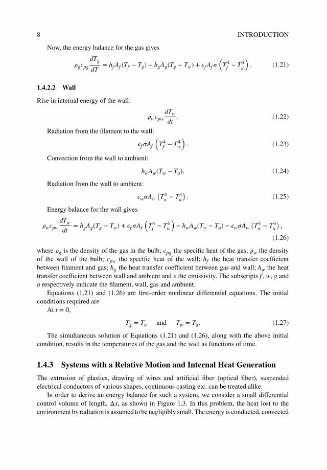
1.4.2 Incandescent Lamp

Figure 1.2 shows an idealized incandescent lamp. The filament is heated to a temperature Tfby an electric current. Heat is convected to the surrounding gas and is radiated to the wall,which also receives heat from the gas by convection. The wall in turn convects and radiatesheat to the ambient at Ta. A formulation of equations, based on energy balance, is necessaryin order to determine the temperature of the gas and the wall with respect to time.

1.4.2.1 Gas

Rise in internal energy of the gas:

𝜌gcpg

dTg

dt. (1.17)

Convection from the filament to the gas:

hf Af (Tf − Tg). (1.18)

Convection from the gas to the wall:

hgAg(Tg − Tw). (1.19)

Radiation from the filament to the gas:

𝜖f Af𝜎

(T4

f − T4g

). (1.20)

8 INTRODUCTION

Now, the energy balance for the gas gives

𝜌gcpg

dTg

dT= hf Af (Tf − Tg) − hgAg(Tg − Tw) + 𝜖f Af𝜎

(T4

f − T4g

). (1.21)

1.4.2.2 Wall

Rise in internal energy of the wall:

𝜌wcpwdTw

dt. (1.22)

Radiation from the filament to the wall:

𝜖f𝜎Af

(T4

f − T4w

). (1.23)

Convection from the wall to ambient:

hwAw(Tw − Ta). (1.24)

Radiation from the wall to ambient:

𝜖w𝜎Aw

(T4

w − T4a

). (1.25)

Energy balance for the wall gives

𝜌wcpwdTw

dt= hgAg(Tg − Tw) + 𝜖f𝜎Af

(T4

f − T4w

)− hwAw(Tw − Ta) − 𝜖w𝜎Aw

(T4

w − T4a

),

(1.26)

where 𝜌g is the density of the gas in the bulb; cpg the specific heat of the gas; 𝜌w the densityof the wall of the bulb; cpw the specific heat of the wall; hf the heat transfer coefficientbetween filament and gas; hg the heat transfer coefficient between gas and wall; hw the heattransfer coefficient between wall and ambient and 𝜖 the emissivity. The subscripts f , w, g anda respectively indicate the filament, wall, gas and ambient.

Equations (1.21) and (1.26) are first-order nonlinear differential equations. The initialconditions required are

At t = 0,

Tg = Ta and Tw = Ta. (1.27)

The simultaneous solution of Equations (1.21) and (1.26), along with the above initialcondition, results in the temperatures of the gas and the wall as functions of time.

1.4.3 Systems with a Relative Motion and Internal Heat Generation

The extrusion of plastics, drawing of wires and artificial fiber (optical fiber), suspendedelectrical conductors of various shapes, continuous casting etc. can be treated alike.

In order to derive an energy balance for such a system, we consider a small differentialcontrol volume of length, Δx, as shown in Figure 1.3. In this problem, the heat lost to theenvironment by radiation is assumed to be negligibly small. The energy is conducted, convected

INTRODUCTION 9

xΔ x

x + dx

me

u

me

q

q

x + dx

x + dx

x

x

hPΔx (T - Ta)

Figure 1.3 Conservation of energy in a moving body.

and transported with the material in motion. With reference to Figure 1.3, we can write thefollowing equations of conservation of energy, that is,

Qx + mex + GAΔx = Qx+dx + mex+dx + hPΔx(T − Ta), (1.28)

where Q = Aq is the total heat; m is the mass flow 𝜌Au and is assumed to be constant; ex isthe specific energy; 𝜌 the density of the material; A the cross-sectional area; P the perimeterof the control volume; G is the heat generated per unit volume and u is the velocity at whichthe material is moving. Using the Taylor series of expansion we obtain

m(ex − ex+dx) = −mdex

dxΔx = −mcp

dTdx

Δx. (1.29)

Note that dex = cpdT at constant pressure. Similarly, using Fourier’s law (Equation (1.1)),

Qx − Qx+dx = −dQx

dx= d

dx

[kA

dTdx

]. (1.30)

On substituting Equations (1.29) and (1.30) into Equation (1.28), we obtain the followingconservation equation,

ddx

[kA

dTdx

]− hP(T − Ta) − 𝜌cpAu

dTdx

+ GA = 0. (1.31)

In the above equation, the first term is derived from the heat diffusion (conduction) withinthe material, the second term is due to convection from the material surface to ambient, thethird term represents the heat transport due to the motion of the material, and finally the lastterm is added to account for heat generation within the body.

10 INTRODUCTION

1.5 Heat Conduction Equation

The determination of temperature distribution in a medium (solid, liquid, gas or combinationof phases) is the main objective of a conduction analysis, that is, to know the temperature inthe medium as a function of space at steady state and as a function of time during the transientstate. Once this temperature distribution is known, the heat flux at any point within the medium,or on its surface, may be computed from Fourier’s law, Equation (1.1). A knowledge of thetemperature distribution within a solid can be used to determine the structural integrity viaa determination of the thermal stresses and distortion. The optimization of the thickness ofan insulating material and the compatibility of any special coatings or adhesives used on thematerial can be studied by knowing the temperature distribution.

We shall now derive the conduction equation in Cartesian coordinates by applying theenergy conservation law to a differential control volume as shown in Figure 1.4. The solution ofthe resulting differential equation, with prescribed boundary conditions, gives the temperaturedistribution in the medium.

The Taylor series expansion gives:

Qx+dx = Qx +𝜕Qx

𝜕xΔx

Qy+dy = Qy +𝜕Qy

𝜕yΔy

Qz+dz = Qz +𝜕Qz

𝜕zΔz. (1.32)

Q

Q

Q

z

y

x Qx+Δx

Qz+ΔzQy+Δy

x

yz

Δy

Δz

Δx

Figure 1.4 A differential control volume for heat conduction analysis.

INTRODUCTION 11

Note that second and higher order terms are neglected in the above equation.The heatgenerated in the control volume is GΔxΔyΔz and the rate of change in energy storage is givenas

𝜌cp(ΔxΔyΔz)𝜕T𝜕t. (1.33)

Now, with reference to Figure 1.4, we can write the energy balance as

”energy inlet + energy generated = energy stored + energy exit”

that is:

(Qx + Qy + Qz) + G(ΔxΔyΔz) = 𝜌(ΔxΔyΔz)𝜕T𝜕t

+ Qx+dx + Qy+dy + Qz+dz. (1.34)

Substituting Equation (1.32) into the previous equation and rearranging results in;

−𝜕Qx

𝜕xΔx −

𝜕Qy

𝜕yΔy −

𝜕Qz

𝜕zΔz + G(ΔxΔyΔz) = 𝜌cp(ΔxΔyΔz)

𝜕T𝜕t. (1.35)

The total heat transfer Q in each direction can be expressed as (area perpendicular to heatflux direction × heat flux):

Qx = (ΔyΔz)qx = −kx(ΔyΔz)𝜕T𝜕x

Qy = (ΔxΔz)qy = −ky(ΔxΔz)𝜕T𝜕y

Qz = (ΔxΔy)qz = −kz(ΔxΔy)𝜕T𝜕z. (1.36)

Substituting Equation (1.36) into Equation (1.35) and dividing by the volume, ΔxΔyΔz,we get

𝜕

𝜕x

[kx𝜕T𝜕x

]+ 𝜕

𝜕y

[ky𝜕T𝜕y

]+ 𝜕

𝜕z

[kz𝜕T𝜕z

]+ G = 𝜌cp

𝜕T𝜕t. (1.37)

Equation (1.37) is the transient heat conduction equation for a stationary system expressedin Cartesian coordinates. The thermal conductivity, k, in the above equation is a vector. In itsmost general form, the thermal conductivity can be expressed as a tensor, that is,

k =⎡⎢⎢⎣

kxx kxy kxzkyx kyy kyzkzx kzy kzz

⎤⎥⎥⎦ . (1.38)

The preceding Equations (1.37) and (1.38) are valid for solving heat conduction problemsin anisotropic materials with directional variation in thermal conductivities. In many situations,however, thermal conductivity can be taken as a nondirectional property, that is, the material

12 INTRODUCTION

is isotropic in nature. In such materials, the heat conduction equation is written as (constantthermal conductivity):

𝜕2T𝜕x2

+ 𝜕2T𝜕y2

+ 𝜕2T𝜕z2

+ Gk= 1𝛼

𝜕T𝜕t

, (1.39)

where 𝛼 = k∕𝜌cp is the thermal diffusivity, which is an important parameter in transient heatconduction analyses. If the analysis is restricted only to steady-state heat conduction withoutheat generation, the equation is reduced to

𝜕2T𝜕x2

+ 𝜕2T𝜕y2

+ 𝜕2T𝜕z2

= 0. (1.40)

For a one-dimensional case, the steady-state heat conduction equation is further reducedto

ddx

(k

dTdx

)= 0. (1.41)

The heat conduction equation for a cylindrical coordinate system is given by

1r𝜕

𝜕r

[krr

𝜕T𝜕r

]+ 1

r2

𝜕

𝜕𝜙

[k𝜙

𝜕T𝜕𝜙

]+ 𝜕

𝜕z

[kz𝜕T𝜕z

]+ G = 𝜌cp

𝜕T𝜕t. (1.42)

In cylindrical coordinates, the heat fluxes can be expressed as

qr = −kr𝜕T𝜕r

q𝜙= −

k𝜙

r𝜕T𝜕𝜙

qz = −kz𝜕T𝜕z

, (1.43)

where r,𝜙 and z are the cylindrical coordinate directions. The heat conduction equation for aspherical coordinate system is given by

1r2

𝜕

𝜕r

[krr2 𝜕T

𝜕r

]+( 1

r2sin2𝜃

)𝜕

𝜕𝜙

[k𝜙

𝜕T𝜕𝜙

]+( 1

r2sin𝜃

)𝜕

𝜕𝜃

[k𝜃sin𝜃

𝜕T𝜕𝜃

]+ G = 𝜌cp

𝜕T𝜕t. (1.44)

The heat fluxes in a spherical coordinate system can be expressed as

qr = −kr𝜕T𝜕r

q𝜙= −

k𝜙

rsin𝜃𝜕T𝜕𝜙

q𝜃= −

k𝜃

r𝜕T𝜕𝜃

, (1.45)

INTRODUCTION 13

where r,𝜙 and 𝜃 are the spherical coordinate directions. It should be noted that for bothcylindrical and spherical coordinate systems (Equations (1.42) and (1.44)) can be derived in asimilar fashion as for Cartesian coordinates by considering the appropriate differential controlvolumes.

1.6 Mass Transfer

When a concentration gradient exists in a fluid mixture, mass transfer takes place from a higherconcentration to a lower concentration location. Such mass transport often takes place at themolecular level in the form of mass diffusion. The mass transport at the macroscopic level isreferred to as mass convection. Thus, the modes of mass transfer are very similar to the firsttwo modes of heat transfer, that is, conduction (diffusion) and convection. Mass diffusion isoften described using Fick’s law of mass transport (Fick 1855). This states that the mass fluxof a constituent per unit area is proportional to the concentration gradient, that is,

JA =mA

A= −DAB

dCA

dx, (1.46)

where mA is the mass flux per unit time, DAB is the diffusion coefficient and CA is the massconcentration of the component A. As seen, this expression is very similar to Fourier’s law ofheat conduction (Equation (1.1)). The convective mass flux per unit area may be defined as

mA

A= hA(CA − CA∞), (1.47)

where hA is the mass transfer coefficient and CA − CA∞ is the concentration difference throughwhich mass transfer occurs. Equation (1.47) is analogous to the Newton’s law of cooling forheat transfer (Equation (1.2)). Further details on mass transfer are given in Chapter 10.

1.7 Boundary and Initial Conditions

The heat conduction equations discussed in Section 1.5 will be complete for any problemonly if the appropriate boundary and initial conditions are stated. With the necessary boundaryand initial conditions, a solution to the heat conduction equation is possible. The boundaryconditions for the conduction equation can be of two types or a combination of these: theDirichlet condition, in which the temperature on the boundaries is known and/or the Neumanncondition, in which the heat flux is imposed, that is (see Figure 1.5):

Dirichlet condition:

T = To on ΓT . (1.48)

Neumann condition:

q = −k𝜕T𝜕n

= q on Γqf . (1.49)

14 INTRODUCTION

Γ

Ω

Γ

Γ

T

qc

q f

Figure 1.5 Boundary conditions.

In the above equations (Equations (1.48) and (1.49)), To is the prescribed temperature; Γthe boundary surface; n is the outward direction normal to the surface and q is the constantflux given. The insulated, or adiabatic, condition can be obtained by substituting q = 0. Theconvective heat transfer boundary condition also falls into the Neumann category and can beexpressed as

− k𝜕T𝜕n

= h(Tw − Ta) on Γqc. (1.50)

It should be observed that the heat conduction equation has second-order terms and hencefaces two types of boundary conditions. Since the time appears as a first-order term, at leastone initial value (i.e., at some instant of time all temperatures must be known) is to be specifiedfor the entire body, that is,

T = T0 all over the domain Ω at t = t0, (1.51)

where t0 is a reference time.The constant or variable temperature conditions are generally easy to implement as tem-

perature is a scalar. However, the implementation of surface fluxes is not as straightforward.Equation (1.49) can be rewritten with direction cosines of the outward normals as

−(

kx𝜕T𝜕x

l + ky𝜕T𝜕y

m + kz𝜕T𝜕z

n

)= q on Γqf . (1.52)

Similarly, Equation (1.50) can be rewritten as

−(

kx𝜕T𝜕x

l + ky𝜕T𝜕y

m + kz𝜕T𝜕z

n

)= h(T − Ta) on Γqc, (1.53)

where l, m and n are the direction cosines of the appropriate outward surface normals.In many industrial applications, for example, wire drawing, crystal growth, continuous

casting, etc., the material will have a motion in space and this motion may be restricted to one