Embed Size (px)
Citation preview


FUNDAMENTALS OFWIRELESS SENSORNETWORKS

Wiley Series on Wireless Communications and Mobile Computing
Series Editors: Dr Xuemin (Sherman) Shen, University of Waterloo, CanadaDr Yi Pan, Georgia State University, USA
The “Wiley Series on Wireless Communications and Mobile Computing” is a series of comprehensive,practical and timely books on wireless communication and network systems. The series focuses ontopics ranging from wireless communication and coding theory to wireless applications and pervasivecomputing. The books provide engineers and other technical professionals, researchers, educators, andadvanced students in these fields with invaluable insight into the latest developments and cutting-edgeresearch.
Other titles in the series:
Misic and Misic: Wireless Personal Area Networks: Performance, Interconnection, and Security withIEEE 802.15.4 , January 2008, 978-0-470-51847-2
Takagi and Walke: Spectrum Requirement Planning in Wireless Communications: Model andMethodology for IMT-Advanced , April 2008, 978-0-470-98647-9
Perez-Fontan and Espineira: Modeling the Wireless Propagation Channel: A simulation approach withMATLAB, August 2008, 978-0-470-72785-0
Ippolito: Satellite Communications Systems Engineering: Atmospheric Effects, Satellite Link Designand System Performance, August 2008, 978-0-470-72527-6
Lin and Sou: Charging for Mobile All-IP Telecommunications , September 2008, 978-0-470-77565-3
Myung and Goodman: Single Carrier FDMA: A New Air Interface for Long Term Evolution , October2008, 978-0-470-72449-1
Wang, Kondi, Luthra and Ci: 4G Wireless Video Communications , April 2009, 978-0-470-77307-9
Cai, Shen and Mark: Multimedia Services in Wireless Internet: Modeling and Analysis , June 2009,978-0-470-77065-8
Stojmenovic: Wireless Sensor and Actuator Networks: Algorithms and Protocols for ScalableCoordination and Data Communication, February 2010, 978-0-470-17082-3
Liu and Weiss, Wideband Beamforming: Concepts and Techniques, March 2010, 978-0-470-71392-1
Riccharia and Westbrook, Satellite Systems for Personal Applications: Concepts and Technology , July2010, 978-0-470-71428-7
Hart, Tao and Zhou: Mobile Multi-hop WiMAX: From Protocol to Performance, October 2010,978-0-470-99399-6
Qian, Muller and Chen: Security in Wireless Networks and Systems, January 2011,978-0-470-512128

FUNDAMENTALS OFWIRELESS SENSORNETWORKSTHEORY AND PRACTICE
Waltenegus DargieTechnical University of Dresden, Germany
Christian PoellabauerUniversity of Notre Dame, USA
A John Wiley and Sons, Ltd., Publication

This edition first published 2010 2010 John Wiley & Sons Ltd.
Registered officeJohn Wiley & Sons Ltd, The Atrium, Southern Gate, Chichester, West Sussex, PO19 8SQ, United Kingdom
For details of our global editorial offices, for customer services and for information about how to apply for permission toreuse the copyright material in this book please see our website at www.wiley.com.
The right of the author to be identified as the author of this work has been asserted in accordance with the Copyright,Designs and Patents Act 1988.
All rights reserved. No part of this publication may be reproduced, stored in a retrieval system, or transmitted, in any formor by any means, electronic, mechanical, photocopying, recording or otherwise, except as permitted by the UK Copyright,Designs and Patents Act 1988, without the prior permission of the publisher.
Wiley also publishes its books in a variety of electronic formats. Some content that appears in print may not be available inelectronic books.
Designations used by companies to distinguish their products are often claimed as trademarks. All brand names and productnames used in this book are trade names, service marks, trademarks or registered trademarks of their respective owners. Thepublisher is not associated with any product or vendor mentioned in this book. This publication is designed to provideaccurate and authoritative information in regard to the subject matter covered. It is sold on the understanding that thepublisher is not engaged in rendering professional services. If professional advice or other expert assistance is required, theservices of a competent professional should be sought.
Library of Congress Cataloging-in-Publication Data:
Dargie, Waltenegus.Fundamentals of wireless sensor networks : theory and practice / Waltenegus Dargie, Christian Poellabauer.
p. cm.Includes index.ISBN 978-0-470-99765-9 (cloth)1. Wireless sensor networks. I. Poellabauer, Christian. II. Title.TK7872.D48D37 2010681’.2 – dc22
2010003984
A catalogue record for this book is available from the British Library.
ISBN 978-0-470-99765-9 (H/B)
Typeset in 10/12 Times by Laserwords Private Limited, Chennai, India.Printed and Bound in Singapore by Markono

To my wife, Kathy,and my children, Joshua and Pheben
Waltenegus Dargie
To my wife, Rumana,and my children, Adam and Maya
Christian Poellabauer


Contents
About the Series Editors xv
Preface xvii
Part One: INTRODUCTION
1 Motivation for a Network of Wireless Sensor Nodes 31.1 Definitions and Background 4
1.1.1 Sensing and Sensors 41.1.2 Wireless Sensor Networks 7
1.2 Challenges and Constraints 91.2.1 Energy 101.2.2 Self-Management 111.2.3 Wireless Networking 111.2.4 Decentralized Management 121.2.5 Design Constraints 121.2.6 Security 131.2.7 Other Challenges 13
Exercises 14References 15
2 Applications 172.1 Structural Health Monitoring 17
2.1.1 Sensing Seismic Events 182.1.2 Single Damage Detection Using Natural Frequencies 192.1.3 Multiple Damage Detection Using Natural Frequencies 192.1.4 Multiple Damage Detection Using Mode Shapes 202.1.5 Coherence 212.1.6 Piezoelectric Effect 222.1.7 Prototypes 24
2.2 Traffic Control 262.2.1 The Sensing Task 262.2.2 Prototypes 30
2.3 Health Care 302.3.1 Available Sensors 322.3.2 Prototypes 32

viii Contents
2.4 Pipeline Monitoring 352.4.1 Prototype 35
2.5 Precision Agriculture 362.5.1 Prototypes 37
2.6 Active Volcano 382.6.1 Prototypes 39
2.7 Underground Mining 402.7.1 Sources of Accidents 412.7.2 The Sensing Task 42
Exercises 42References 44
3 Node Architecture 473.1 The Sensing Subsystem 48
3.1.1 Analog-to-Digital Converter 483.2 The Processor Subsystem 51
3.2.1 Architectural Overview 523.2.2 Microcontroller 543.2.3 Digital Signal Processor 543.2.4 Application-Specific Integrated Circuit 553.2.5 Field Programmable Gate Array 563.2.6 Comparison 57
3.3 Communication Interfaces 583.3.1 Serial Peripheral Interface 583.3.2 Inter-Integrated Circuit 593.3.3 Summary 61
3.4 Prototypes 623.4.1 The IMote Node Architecture 633.4.2 The XYZ Node Architecture 643.4.3 The Hogthrob Node Architecture 65
Exercises 66References 68
4 Operating Systems 694.1 Functional Aspects 70
4.1.1 Data Types 704.1.2 Scheduling 704.1.3 Stacks 714.1.4 System Calls 714.1.5 Handling Interrupts 714.1.6 Multithreading 724.1.7 Thread-Based vs Event-Based Programming 724.1.8 Memory Allocation 73
4.2 Nonfunctional Aspects 734.2.1 Separation of Concern 734.2.2 System Overhead 74

Contents ix
4.2.3 Portability 744.2.4 Dynamic Reprogramming 74
4.3 Prototypes 754.3.1 TinyOS 754.3.2 SOS 784.3.3 Contiki 804.3.4 LiteOS 85
4.4 Evaluation 88Exercises 90References 91
Part Two: BASIC ARCHITECTURAL FRAMEWORK
5 Physical Layer 955.1 Basic Components 955.2 Source Encoding 96
5.2.1 The Efficiency of a Source Encoder 985.2.2 Pulse Code Modulation and Delta Modulation 100
5.3 Channel Encoding 1015.3.1 Types of Channels 1035.3.2 Information Transmission over a Channel 1045.3.3 Error Recognition and Correction 106
5.4 Modulation 1065.4.1 Modulation Types 1065.4.2 Quadratic Amplitude Modulation 1145.4.3 Summary 117
5.5 Signal Propagation 117Exercises 119References 123
6 Medium Access Control 1256.1 Overview 125
6.1.1 Contention-Free Medium Access 1276.1.2 Contention-Based Medium Access 127
6.2 Wireless MAC Protocols 1286.2.1 Carrier Sense Multiple Access 1296.2.2 Multiple Access with Collision Avoidance (MACA) and MACAW 1296.2.3 MACA By Invitation 1306.2.4 IEEE 802.11 1306.2.5 IEEE 802.15.4 and ZigBee 132
6.3 Characteristics of MAC Protocols in Sensor Networks 1336.3.1 Energy Efficiency 1336.3.2 Scalability 1346.3.3 Adaptability 134

x Contents
6.3.4 Low Latency and Predictability 1356.3.5 Reliability 135
6.4 Contention-Free MAC Protocols 1356.4.1 Characteristics 1366.4.2 Traffic-Adaptive Medium Access 1366.4.3 Y-MAC 1376.4.4 DESYNC-TDMA 1396.4.5 Low-Energy Adaptive Clustering Hierarchy 1406.4.6 Lightweight Medium Access Control 143
6.5 Contention-Based MAC Protocols 1446.5.1 Power Aware Multi-Access with Signaling 1446.5.2 Sensor MAC 1466.5.3 Timeout MAC 1466.5.4 Pattern MAC 1486.5.5 Routing-Enhanced MAC 1496.5.6 Data-Gathering MAC 1516.5.7 Preamble Sampling and WiseMAC 1526.5.8 Receiver-Initiated MAC 153
6.6 Hybrid MAC Protocols 1546.6.1 Zebra MAC 1546.6.2 Mobility Adaptive Hybrid MAC 156
6.7 Summary 157Exercises 157References 161
7 Network Layer 1637.1 Overview 1637.2 Routing Metrics 165
7.2.1 Commonly Used Metrics 1667.3 Flooding and Gossiping 1687.4 Data-Centric Routing 170
7.4.1 Sensor Protocols for Information via Negotiation 1707.4.2 Directed Diffusion 1727.4.3 Rumor Routing 1747.4.4 Gradient-Based Routing 175
7.5 Proactive Routing 1767.5.1 Destination-Sequenced Distance Vector 1767.5.2 Optimized Link State Routing 177
7.6 On-Demand Routing 1787.6.1 Ad Hoc On-Demand Distance Vector 1787.6.2 Dynamic Source Routing 179
7.7 Hierarchical Routing 1807.8 Location-Based Routing 183
7.8.1 Unicast Location-Based Routing 1837.8.2 Multicast Location-Based Routing 1887.8.3 Geocasting 189

Contents xi
7.9 QoS-Based Routing Protocols 1927.9.1 Sequential Assignment Routing 1927.9.2 SPEED 1937.9.3 Multipath Multi-SPEED 194
7.10 Summary 196Exercises 197References 203
Part Three: NODE AND NETWORK MANAGEMENT
8 Power Management 2078.1 Local Power Management Aspects 208
8.1.1 Processor Subsystem 2088.1.2 Communication Subsystem 2098.1.3 Bus Frequency and RAM Timing 2108.1.4 Active Memory 2108.1.5 Power Subsystem 212
8.2 Dynamic Power Management 2168.2.1 Dynamic Operation Modes 2168.2.2 Dynamic Scaling 2198.2.3 Task Scheduling 222
8.3 Conceptual Architecture 2228.3.1 Architectural Overview 223
Exercises 225References 227
9 Time Synchronization 2299.1 Clocks and the Synchronization Problem 2299.2 Time Synchronization in Wireless Sensor Networks 231
9.2.1 Reasons for Time Synchronization 2319.2.2 Challenges for Time Synchronization 232
9.3 Basics of Time Synchronization 2349.3.1 Synchronization Messages 2349.3.2 Nondeterminism of Communication Latency 236
9.4 Time Synchronization Protocols 2379.4.1 Reference Broadcasts Using Global Sources of Time 2379.4.2 Lightweight Tree-Based Synchronization 2389.4.3 Timing-sync Protocol for Sensor Networks 2399.4.4 Flooding Time Synchronization Protocol 2409.4.5 Reference-Broadcast Synchronization 2429.4.6 Time-Diffusion Synchronization Protocol 2449.4.7 Mini-Sync and Tiny-Sync 245
Exercises 246References 247

xii Contents
10 Localization 24910.1 Overview 24910.2 Ranging Techniques 250
10.2.1 Time of Arrival 25010.2.2 Time Difference of Arrival 25110.2.3 Angle of Arrival 25110.2.4 Received Signal Strength 252
10.3 Range-Based Localization 25210.3.1 Triangulation 25210.3.2 Trilateration 25310.3.3 Iterative and Collaborative Multilateration 25510.3.4 GPS-Based Localization 256
10.4 Range-Free Localization 25810.4.1 Ad Hoc Positioning System (APS) 25810.4.2 Approximate Point in Triangulation 25910.4.3 Localization Based on Multidimensional Scaling 260
10.5 Event-Driven Localization 26210.5.1 The Lighthouse Approach 26210.5.2 Multi-Sequence Positioning 263
Exercises 264References 266
11 Security 26711.1 Fundamentals of Network Security 26711.2 Challenges of Security in Wireless Sensor Networks 26911.3 Security Attacks in Sensor Networks 270
11.3.1 Denial-of-Service 27011.3.2 Attacks on Routing 27211.3.3 Attacks on Transport Layer 27211.3.4 Attacks on Data Aggregation 27311.3.5 Privacy Attacks 273
11.4 Protocols and Mechanisms for Security 27411.4.1 Symmetric and Public Key Cryptography 27411.4.2 Key Management 27411.4.3 Defenses Against DoS Attacks 27511.4.4 Defenses Against Aggregation Attacks 27611.4.5 Defenses Against Routing Attacks 27711.4.6 Security Protocols for Sensor Networks 27811.4.7 TinySec 27911.4.8 Localized Encryption and Authentication Protocol 280
11.5 IEEE 802.15.4 and ZigBee Security 28011.6 Summary 281Exercises 282References 283

Contents xiii
12 Sensor Network Programming 28512.1 Challenges in Sensor Network Programming 28512.2 Node-Centric Programming 286
12.2.1 nesC Language 28612.2.2 TinyGALS 28912.2.3 Sensor Network Application Construction Kit 29112.2.4 Thread-Based Model 292
12.3 Macroprogramming 29312.3.1 Abstract Regions 29312.3.2 EnviroTrack 29312.3.3 Database Approaches 294
12.4 Dynamic Reprogramming 29512.5 Sensor Network Simulators 297
12.5.1 Network Simulator Tools and Environments 297Exercises 299References 300
Index 303


About the Series EditorsXuemin (Sherman) Shen (M’97-SM’02) received the B.Scdegree in electrical engineering from Dalian Maritime Univer-sity, China in 1982, and the M.Sc. and Ph.D. degrees (bothin electrical engineering) from Rutgers University, New Jer-sey, USA, in 1987 and 1990 respectively. He is a Professorand University Research Chair, and the Associate Chair forGraduate Studies, Department of Electrical and Computer Engi-neering, University of Waterloo, Canada. His research focuseson mobility and resource management in interconnected wire-less/wired networks, UWB wireless communications systems,wireless security, and ad hoc and sensor networks. He is a co-author of three books, and has published more than 300 papers
and book chapters in wireless communications and networks, control and filtering. Dr. Shenserves as a Founding Area Editor for IEEE Transactions on Wireless Communications;Editor-in-Chief for Peer-to-Peer Networking and Application; Associate Editor for IEEETransactions on Vehicular Technology; KICS/IEEE Journal of Communications and Net-works, Computer Networks; ACM/Wireless Networks; and Wireless Communications andMobile Computing (Wiley), etc. He has also served as Guest Editor for IEEE JSAC, IEEEWireless Communications, and IEEE Communications Magazine. Dr. Shen received theExcellent Graduate Supervision Award in 2006, and the Outstanding Performance Award in2004 from the University of Waterloo, the Premier’s Research Excellence Award (PREA)in 2003 from the Province of Ontario, Canada, and the Distinguished Performance Awardin 2002 from the Faculty of Engineering, University of Waterloo. Dr. Shen is a registeredProfessional Engineer of Ontario, Canada.
Dr. Yi Pan is the Chair and a Professor in the Department ofComputer Science at Georgia State University, USA. Dr. Panreceived his B.Eng. and M.Eng. degrees in computer engineeringfrom Tsinghua University, China, in 1982 and 1984, respectively,and his Ph.D. degree in computer science from the University ofPittsburgh, USA, in 1991. Dr. Pan’s research interests includeparallel and distributed computing, optical networks, wirelessnetworks, and bioinformatics. Dr. Pan has published more than100 journal papers with over 30 papers published in various IEEEjournals. In addition, he has published over 130 papers in refer-eed conferences (including IPDPS, ICPP, ICDCS, INFOCOM,and GLOBECOM). He has also co-edited over 30 books. Dr. Pan

xvi About the Series Editors
has served as an editor-in-chief or an editorial board member for 15 journals including fiveIEEE Transactions and has organized many international conferences and workshops. Dr.Pan has delivered over 10 keynote speeches at many international conferences. Dr. Pan is anIEEE Distinguished Speaker (2000–2002), a Yamacraw Distinguished Speaker (2002), anda Shell Oil Colloquium Speaker (2002). He is listed in Men of Achievement, Who’s Who inAmerica, Who’s Who in American Education, Who’s Who in Computational Science andEngineering, and Who’s Who of Asian Americans.

PrefaceRapid advances in the areas of sensor design, information technologies, and wireless net-works have paved the way for the proliferation of wireless sensor networks. These networkshave the potential to interface the physical world with the virtual (computing) world onan unprecedented scale and provide practical usefulness in developing a large number ofapplications, including the protection of civil infrastructures, habitat monitoring, precisionagriculture, toxic gas detection, supply chain management, and health care. However, thedesign of wireless sensor networks introduces formidable challenges, since the requiredbody of knowledge encompasses a whole range of topics in the field of electrical and com-puter engineering, as well as computer science.
Wireless sensor networks are currently being offered as a subject at advanced undergrad-uate and graduate levels at many universities around the world. Moreover, they are the focusof countless graduate theses and student projects. Therefore, this book is primarily written asa textbook aimed at students of engineering and computer science. It provides an introduc-tion into the fundamental concepts and building blocks of wireless sensor network design.An attempt has been made to maintain a balance between theory and practice, as well asestablished practices and the latest developments. At the end of each chapter, a number ofpractical questions and exercises are given to help the students to assess their understandingof the main concepts and arguments presented in the chapter. Furthermore, the chapters andparts of the book are sufficiently modular to provide flexibility in course design.
The book will also be useful to the professional interested in this field. It is suitable for self-study and can serve as an essential reference. For such a reader, the material can be viewedas a tutorial in the basic concepts and surveys of recent research results and technologicaldevelopments.
Structure of the Book
This book provides an introduction to the fundamental concepts and principles of wirelesssensor networks (WSNs) and a survey of protocols, algorithms, and technologies at differentlayers of a sensor system, including the network protocol stack, middleware, and applicationlevel.
The text is broken into three parts. In Part One, Introduction, Chapter 1 provides anoverview of WSN applications, sensor nodes, and basic system structure. Chapter 2 con-tinues the introduction into the WSN domain by providing an overview of representativesensor network applications. Chapter 3 presents different node architectures and discussesin detail the sensing and processing subsystems as well as communication interfaces. More-over, it provides several examples of representative prototype implementations. Chapter 4
xviii Preface
describes functional and nonfunctional aspects of operating systems and provides a surveyof state-of-the-art examples.
Part Two, Basic Architectural Framework, provides a detailed discussion of proto-cols and algorithms used at different network protocol layers in sensor systems. The designchoices at these layers significantly impact the operation and resource efficiency of sensornodes and networks. Chapter 5 begins this discussion with an introduction into physicallayer architectures and concepts. Since the wireless medium is shared between many sen-sor nodes, MAC-layer protocols are required to arbitrate access to the wireless channels.MAC-layer solutions are discussed in Chapter 6. Chapter 7 discusses multi-hop communi-cations in WSNs and the associated challenges. It also surveys existing and proposed routingprotocols.
Part Three, Node and Network Management, discusses several additional techniquesand presents solutions for a variety of challenges. Chapter 8 begins the discussion withan overview of power management techniques for wireless sensor networks. When multi-ple sensor nodes observe the same event in the physical world, it is important to correctlycorrelate these observations from the different sensors. This requires the clocks of the sen-sor nodes to be synchronized with each other. Synchronized clocks are also required by avariety of protocols and algorithms, e.g., many MAC protocols rely on accurate timing toensure that no two nodes transmit packets at the same time. Therefore, Chapter 9 introducesthe concept of time synchronization and provides an overview of several synchronizationstrategies. For many sensor network applications, it is essential that sensor nodes estimatetheir own position, either using absolute coordinates (e.g., using GPS) or relative to othernodes or landmarks in the environment. Chapter 10 presents a variety of localization strate-gies and compares their tradeoffs. Wireless sensor networks pose several security challengesdue to the nature of many sensor applications (military, emergency response) and the uniquecharacteristics of sensor networks (e.g., scale and unattended operation). Therefore, secu-rity challenges and defenses against attacks on sensor networks are discussed in Chapter 11.Finally, Chapter 12 concludes the book with a description of development environmentsand programming techniques for sensor networks, including an overview of frequently usedsensor network simulators.

Part OneIntroduction


1Motivation for a Network ofWireless Sensor NodesSensors link the physical with the digital world by capturing and revealing real-world phe-nomena and converting these into a form that can be processed, stored, and acted upon. Inte-grated into numerous devices, machines, and environments, sensors provide a tremendoussocietal benefit. They can help to avoid catastrophic infrastructure failures, conserve pre-cious natural resources, increase productivity, enhance security, and enable new applicationssuch as context-aware systems and smart home technologies. The phenomenal advancesin technologies such as very large scale integration (VLSI), microelectromechanical sys-tems (MEMS), and wireless communications further contribute to the widespread use ofdistributed sensor systems. For example, the impressive developments in semiconductortechnologies continue to produce microprocessors with increasing processing capacities,while at the same time shrinking in size. The miniaturization of computing and sensingtechnologies enables the development of tiny, low-power, and inexpensive sensors, actu-ators, and controllers. Further, embedded computing systems (i.e., systems that typicallyinteract closely with the physical world and are designed to perform only a limited numberof dedicated functions) continue to find application in an increasing number of areas. Whiledefense and aerospace systems still dominate the market, there is an increasing focus on sys-tems to monitor and protect civil infrastructure (such as bridges and tunnels), the nationalpower grid, and pipeline infrastructure. Networks of hundreds of sensor nodes are alreadybeing used to monitor large geographic areas for modeling and forecasting environmentalpollution and flooding, collecting structural health information on bridges using vibrationsensors, and controlling usage of water, fertilizers, and pesticides to improve crop healthand quantity.
This book provides a thorough introduction to the fundamental aspects of wireless sensornetworks (WSNs), covering both theoretical concepts and practical aspects of networktechnologies and protocols, operating systems, middleware, sensor programming, and secu-rity. The book is targeted at researchers, students, and practitioners alike, with the goal ofhelping them to gain an understanding of the challenges and promises of this exciting field.It has been written primarily as a textbook for graduate or advanced undergraduate coursesin wireless sensor networks. Each chapter ends with a number of exercises and questionsthat will allow students to practice the described concepts and techniques. As the field ofwireless sensor networks is based on numerous other domains, it is recommended that
Fundamentals of Wireless Sensor Networks: Theory and Practice Waltenegus Dargie and Christian Poellabauer 2010 John Wiley & Sons, Ltd

4 Fundamentals of Wireless Sensor Networks
students have taken courses such as networking and operating systems (or comparablecourses) before they take a course on sensor networks. Also, some topics covered in thisbook (e.g., security) assume previous knowledge in other areas or require that an instructorprovides an introduction into the basics of these areas before teaching these topics.
1.1 Definitions and Background
1.1.1 Sensing and Sensors
Sensing is a technique used to gather information about a physical object or process,including the occurrence of events (i.e., changes in state such as a drop in temperature orpressure). An object performing such a sensing task is called a sensor . For example, thehuman body is equipped with sensors that are able to capture optical information from theenvironment (eyes), acoustic information such as sounds (ears), and smells (nose). Theseare examples of remote sensors , that is, they do not need to touch the monitored objectto gather information. From a technical perspective, a sensor is a device that translatesparameters or events in the physical world into signals that can be measured and analyzed.Another commonly used term is transducer , which is often used to describe a device thatconverts energy from one form into another. A sensor, then, is a type of transducer that con-verts energy in the physical world into electrical energy that can be passed to a computingsystem or controller. An example of the steps performed in a sensing (or data acquisition)task is shown in Figure 1.1. Phenomena in the physical world (often referred to as process ,system, or plant) are observed by a sensor device. The resulting electrical signals are oftennot ready for immediate processing, therefore they pass through a signal conditioningstage. Here, a variety of operations can be applied to the sensor signal to prepare it forfurther use. For example, signals often require amplification (or attenuation) to change thesignal magnitude to better match the range of the following analog-to-digital conversion.Further, signal conditioning often applies filters to the signal to remove unwanted noisewithin certain frequency ranges (e.g., highpass filters can be used to remove 50 or 60 Hznoise picked up by surrounding power lines). After conditioning, the analog signal istransformed into a digital signal using an analog-to-digital converter (ADC). The signal isnow available in a digital form and ready for further processing, storing, or visualization.
Processing
ConverterActuator Conditioning
ConverterConditioning
Sensing
Actuation
Signal
PRO
CE
SS
Digital–to–Analog
Analog–to–DigitalSensor
Figure 1.1 Data acquisition and actuation.

Motivation for a Network of Wireless Sensor Nodes 5
Many wireless sensor networks also include actuators which allow them to directly con-trol the physical world. For example, an actuator can be a valve controlling the flow of hotwater, a motor that opens or closes a door or window, or a pump that controls the amount offuel injected into an engine. Such a wireless sensor and actuator network (WSAN) takescommands from the processing device (controller) and transforms these commands intoinput signals for the actuator, which then interacts with a physical process, thereby forminga closed control loop (also shown in Figure 1.1).
1.1.1.1 Sensor Classifications
Which sensors should be chosen for an application depends on the physical property to bemonitored, for example, such properties include temperature, pressure, light, or humidity.Table 1.1 summarizes some common physical properties, including examples of sensingtechnologies that are used to capture them. Besides physical properties, the classification ofsensors can be based on a variety of other methods, for example, whether they require anexternal power supply. If the sensors require external power, they are referred to as activesensors. That is, they must emit some kind of energy (e.g., microwaves, light, sound) totrigger a response or to detect a change in the energy of the transmitted signal. On the otherhand, passive sensors detect energy in the environment and derive their power from thisenergy input – for example, passive infrared (PIR) sensors measure infrared light radiatingfrom objects in the proximity.
The classification of sensors can also be based on the methods they apply and the elec-trical phenomena they utilize to convert physical properties into electrical signals. Resistivesensors rely on changes to a conductor’s electrical resistivity, ρ, based on physical propertiessuch as temperature. The resistance, R, of a conductor can be determined as:
R = l × ρ
A(1.1)
where l is the length of the conductor and A is the area of the cross-section. For example, thewell-known Wheatstone bridge (Figure 1.2) is a simple circuit that can be used to converta physical property into an observable electric effect. In this bridge, R1, R2, and R3 are
Table 1.1 Classification and examples of sensors
Type Examples
Temperature Thermistors, thermocouplesPressure Pressure gauges, barometers, ionization gaugesOptical Photodiodes, phototransistors, infrared sensors, CCD sensorsAcoustic Piezoelectric resonators, microphonesMechanical Strain gauges, tactile sensors, capacitive diaphragms, piezoresistive cellsMotion, vibration Accelerometers, gyroscopes, photo sensorsFlow Anemometers, mass air flow sensorsPosition GPS, ultrasound-based sensors, infrared-based sensors, inclinometersElectromagnetic Hall-effect sensors, magnetometersChemical pH sensors, electrochemical sensors, infrared gas sensorsHumidity Capacitive and resistive sensors, hygrometers, MEMS-based humidity sensorsRadiation Ionization detectors, Geiger–Mueller counters

6 Fundamentals of Wireless Sensor Networks
VOUT
Rx
R3
R2
R1
+
–VCC
Figure 1.2 Wheatstone bridge circuit.
resistors of known resistance (where the resistance of R2 is adjustable) and Rx is a resistor ofunknown value. If the ratio R2/R1 is identical to the ratio Rx/R3, the measured voltage VOUT
will be zero. However, if the resistance of Rx changes (e.g., due to changes in temperature),there will be an imbalance, which will be reflected by a change in voltage VOUT. In general,the relationship between the measured voltage VOUT, the resistors, and the supply voltage(VCC) can be expressed as:
VOUT = VCC ×(
Rx
R3 + Rx
− R2
R1 + R2
)(1.2)
A similar principle can be applied to capacitive sensors, which can be used to measuremotion, proximity, acceleration, pressure, electric fields, chemical compositions, and liquiddepth. For example, in the parallel plate model, that is, a capacitor consisting of two parallelconductive plates separated by a dielectric with a certain permittivity ε, the capacitance isdetermined as:
C = ε × A
d(1.3)
where A is the plate area and d is the distance between the two plates. Similar to the resistivemodel, changes in any of these parameters will change the capacitance. For example, if pres-sure is applied to one of the two plates, the separation d can be reduced, thereby increasingthe capacitance. Similarly, a change in the permittivity of the dielectric can be caused by anincrease in temperature or humidity, thereby resulting in a change in capacitance.
Inductive sensors are based on the electrical principle of inductance, that is, where anelectromagnetic force is induced by a fluctuating current. Inductance is determined by thedimensions of the sensor (cross-sectional area, length of coil), the number of turns of thecoil, and the permeability of the core. Changes in any of these parameters (e.g., caused bymovements of the core within the coil) change the inductance. Inductive sensors are oftenused to measure proximity, position, force, pressure, temperature, and acceleration.
Finally, piezoelectric sensors use the piezoelectric effect of some materials (e.g.,crystals and certain ceramics) to measure pressure, force, strain, and acceleration. Whena pressure is applied to such a material, it causes a mechanical deformation and adisplacement of charges, proportional to the amount of pressure. The main advantage ofpiezoelectric devices over other approaches is that the piezoelectric effect is not sensitiveto electromagnetic fields or radiation.

Motivation for a Network of Wireless Sensor Nodes 7
1.1.2 Wireless Sensor Networks
While many sensors connect to controllers and processing stations directly (e.g., using localarea networks), an increasing number of sensors communicate the collected data wirelesslyto a centralized processing station. This is important since many network applicationsrequire hundreds or thousands of sensor nodes, often deployed in remote and inaccessibleareas. Therefore, a wireless sensor has not only a sensing component, but also on-boardprocessing, communication, and storage capabilities. With these enhancements, a sensornode is often not only responsible for data collection, but also for in-network analysis,correlation, and fusion of its own sensor data and data from other sensor nodes. When manysensors cooperatively monitor large physical environments, they form a wireless sensornetwork (WSN). Sensor nodes communicate not only with each other but also with a basestation (BS) using their wireless radios, allowing them to disseminate their sensor data toremote processing, visualization, analysis, and storage systems. For example, Figure 1.3shows two sensor fields monitoring two different geographic regions and connecting to theInternet using their base stations.
The capabilities of sensor nodes in a WSN can vary widely, that is, simple sensornodes may monitor a single physical phenomenon, while more complex devices maycombine many different sensing techniques (e.g., acoustic, optical, magnetic). They canalso differ in their communication capabilities, for example, using ultrasound, infrared, orradio frequency technologies with varying data rates and latencies. While simple sensorsmay only collect and communicate information about the observed environment, morepowerful devices (i.e., devices with large processing, energy, and storage capacities)may also perform extensive processing and aggregation functions. Such devices oftenassume additional responsibilities in a WSN, for example, they may form communicationbackbones that can be used by other resource-constrained sensor devices to reach the
Base Station
Sensor
Processing
Sensor Field 1 Sensor Field 2
Internet
Mining
Analysis
Storage
Figure 1.3 Wireless sensor networks.

8 Fundamentals of Wireless Sensor Networks
base station. Finally, some devices may have access to additional supporting technologies,for example, Global Positioning System (GPS) receivers, allowing them to accuratelydetermine their position. However, such systems often consume too much energy to befeasible for low-cost and low-power sensor nodes.
1.1.2.1 History of Wireless Sensor Networks
As with many other technologies, the military has been a driving force behind the develop-ment of wireless sensor networks. For example, in 1978, the Defense Advanced ResearchProjects Agency (DARPA) organized the Distributed Sensor Nets Workshop (DAR 1978),focusing on sensor network research challenges such as networking technologies, signalprocessing techniques, and distributed algorithms. DARPA also operated the DistributedSensor Networks (DSN) program in the early 1980s, which was then followed by the SensorInformation Technology (SensIT) program.
In collaboration with the Rockwell Science Center, the University of California at LosAngeles proposed the concept of Wireless Integrated Network Sensors or WINS (Pottie2001). One outcome of the WINS project was the Low Power Wireless Integrated Microsen-sor (LWIM), produced in 1996 (Bult et al. 1996). This smart sensing system was based ona CMOS chip, integrating multiple sensors, interface circuits, digital signal processing cir-cuits, wireless radio, and microcontroller onto a single chip. The Smart Dust project (Kahnet al. 1999) at the University of California at Berkeley focused on the design of extremelysmall sensor nodes called motes . The goal of this project was to demonstrate that a com-plete sensor system can be integrated into tiny devices, possibly the size of a grain of sandor even a dust particle. The PicoRadio project (Rabaey et al. 2000) by the Berkeley Wire-less Research Center (BWRC) focuses on the development of low-power sensor devices,whose power consumption is so small that they can power themselves from energy sourcesof the operating environment, such as solar or vibrational energy. The MIT µAMPS (micro-Adaptive Multidomain Power-aware Sensors) project also focuses on low-power hardwareand software components for sensor nodes, including the use of microcontrollers capable ofdynamic voltage scaling and techniques to restructure data processing algorithms to reducepower requirements at the software level (Calhoun et al. 2005).
While these previous efforts are mostly driven by academic institutions, over the lastdecade a number of commercial efforts have also appeared (many based on some of the aca-demic efforts described above), including companies such as Crossbow (www.xbow.com),Sensoria (www.sensoria.com), Worldsens (http://worldsens.citi.insa-lyon.fr), Dust Net-works (http://www.dustnetworks.com), and Ember Corporation (http://www.ember.com).These companies provide the opportunity to purchase sensor devices ready for deploymentin a variety of application scenarios along with various management tools for programming,maintenance, and sensor data visualization.
1.1.2.2 Communication in a WSN
The well-known IEEE 802.11 family of standards was introduced in 1997 and is the mostcommon wireless networking technology for mobile systems. It uses different frequencybands, for example, the 2.4-GHz band is used by IEEE 802.11b and IEEE 802.11g, while theIEEE 802.11a protocol uses the 5-GHz frequency band. IEEE 802.11 was frequently used inearly wireless sensor networks and can still be found in current networks when bandwidth

Motivation for a Network of Wireless Sensor Nodes 9
Base Station
Single-Hop Multi-Hop
Sensor
Aggregation Node
Figure 1.4 Single-hop versus multi-hop communication in sensor networks.
demands are high (e.g., for multimedia sensors). However, the high-energy overheads ofIEEE 802.11-based networks makes this standard unsuitable for low-power sensor networks.Typical data rate requirements in sensor networks are comparable to the bandwidths pro-vided by dial-up modems, therefore the data rates provided by IEEE 802.11 are typicallymuch higher than needed. This has led to the development of a variety of protocols that bet-ter satisfy the networks’ need for low power consumption and low data rates. For example,the IEEE 802.15.4 protocol (Gutierrez et al. 2001) has been designed specifically for short-range communications in low-power sensor networks and is supported by most academicand commercial sensor nodes.
When the transmission ranges of the radios of all sensor nodes are large enough and thesensors can transmit their data directly to the base station, they can form a star topology asshown on the left in Figure 1.4. In this topology, each sensor node communicates directlywith the base station using a single hop. However, sensor networks often cover large geo-graphic areas and radio transmission power should be kept at a minimum in order to conserveenergy; consequently, multi-hop communication is the more common case for sensor net-works (shown on the right in Figure 1.4). In this mesh topology , sensor nodes must notonly capture and disseminate their own data, but also serve as relays for other sensor nodes,that is, they must collaborate to propagate sensor data towards the base station. This rout-ing problem, that is, the task of finding a multi-hop path from a sensor node to the basestation, is one of the most important challenges and has received immense attention fromthe research community. When a node serves as a relay for multiple routes, it often has theopportunity to analyze and pre-process sensor data in the network, which can lead to theelimination of redundant information or aggregation of data that may be smaller than theoriginal data.
1.2 Challenges and Constraints
While sensor networks share many similarities with other distributed systems, they aresubject to a variety of unique challenges and constraints. These constraints impact thedesign of a WSN, leading to protocols and algorithms that differ from their counterparts inother distributed systems. This section describes the most important design constraints ofa WSN.
10 Fundamentals of Wireless Sensor Networks
1.2.1 Energy
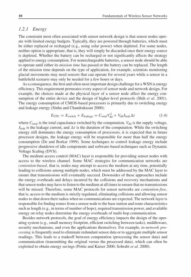
The constraint most often associated with sensor network design is that sensor nodes oper-ate with limited energy budgets. Typically, they are powered through batteries, which mustbe either replaced or recharged (e.g., using solar power) when depleted. For some nodes,neither option is appropriate, that is, they will simply be discarded once their energy sourceis depleted. Whether the battery can be recharged or not significantly affects the strategyapplied to energy consumption. For nonrechargeable batteries, a sensor node should be ableto operate until either its mission time has passed or the battery can be replaced. The lengthof the mission time depends on the type of application, for example, scientists monitoringglacial movements may need sensors that can operate for several years while a sensor in abattlefield scenario may only be needed for a few hours or days.
As a consequence, the first and often most important design challenge for a WSN is energyefficiency. This requirement permeates every aspect of sensor node and network design. Forexample, the choices made at the physical layer of a sensor node affect the energy con-sumption of the entire device and the design of higher-level protocols (Shih et al. 2001).The energy consumption of CMOS-based processors is primarily due to switching energyand leakage energy (Sinha and Chandrakasan 2000):
ECPU = Eswitch + Eleakage = CtotalV2
dd + VddIleak�t (1.4)
where Ctotal is the total capacitance switched by the computation, Vdd is the supply voltage,Ileak is the leakage current, and �t is the duration of the computation. While the switchingenergy still dominates the energy consumption of processors, it is expected that in futureprocessor designs, the leakage energy will be responsible for more than half the energyconsumption (De and Borkar 1999). Some techniques to control leakage energy includeprogressive shutdown of idle components and software-based techniques such as DynamicVoltage Scaling (DVS).
The medium access control (MAC) layer is responsible for providing sensor nodes withaccess to the wireless channel. Some MAC strategies for communication networks arecontention-based , that is, nodes may attempt to access the medium at any time, potentiallyleading to collisions among multiple nodes, which must be addressed by the MAC layer toensure that transmissions will eventually succeed. Downsides of these approaches includethe energy overheads and delays incurred by the collisions and recovery mechanisms andthat sensor nodes may have to listen to the medium at all times to ensure that no transmissionswill be missed. Therefore, some MAC protocols for sensor networks are contention-free,that is, access to the medium is strictly regulated, eliminating collisions and allowing sensornodes to shut down their radios when no communications are expected. The network layer isresponsible for finding routes from a sensor node to the base station and route characteristicssuch as length (e.g., in terms of number of hops), required transmission power, and availableenergy on relay nodes determine the energy overheads of multi-hop communication.
Besides network protocols, the goal of energy efficiency impacts the design of the oper-ating system (e.g., small memory footprint, efficient switching between tasks), middleware,security mechanisms, and even the applications themselves. For example, in-network pro-cessing is frequently used to eliminate redundant sensor data or to aggregate multiple sensorreadings. This leads to a tradeoff between computation (processing the sensor data) andcommunication (transmitting the original versus the processed data), which can often beexploited to obtain energy savings (Pottie and Kaiser 2000; Sohrabi et al. 2000).

Motivation for a Network of Wireless Sensor Nodes 11
1.2.2 Self-Management
It is the nature of many sensor network applications that they must operate in remote areasand harsh environments, without infrastructure support or the possibility for maintenanceand repair. Therefore, sensor nodes must be self-managing in that they configure themselves,operate and collaborate with other nodes, and adapt to failures, changes in the environment,and changes in the environmental stimuli without human intervention.
1.2.2.1 Ad Hoc Deployment
Many wireless sensor network applications do not require predetermined and engineeredlocations of individual sensor nodes. This is particularly important for networks beingdeployed in remote or inaccessible areas. For example, sensors serving the assessment ofbattlefield or disaster areas could be thrown from airplanes over the areas of interest, butmany sensor nodes may not survive such a drop and may never be able to begin their sensingactivities. However, the surviving nodes must autonomously perform a variety of setupand configuration steps, including the establishment of communications with neighboringsensor nodes, determining their positions, and the initiation of their sensing responsibilities.The mode of operation of sensor nodes can differ based on such information, for example,a node’s location and the number or identities of its neighbors may determine the amountand type of information it will generate and forward on behalf of other nodes.
1.2.2.2 Unattended Operation
Many sensor networks, once deployed, must operate without human intervention, that is,configuration, adaptation, maintenance, and repair must be performed in an autonomousfashion. For example, sensor nodes are exposed to both system dynamics and environmentaldynamics, which pose a significant challenge for building reliable sensor networks (Cerpaand Estrin 2004). A self-managing device will monitor its surroundings, adapt to changesin the environment, and cooperate with neighboring devices to form topologies or agreeon sensing, processing, and communication strategies (Mills 2007). Self-management cantake place in a variety of forms. Self-organization is the term frequently used to describea network’s ability to adapt configuration parameters based on system and environmentalstate. For example, a sensor device can choose its transmission power to maintain a certaindegree of connectivity (i.e., with increasing transmission power it is more likely that a nodewill reach more neighbors). Self-optimization refers to a device’s ability to monitor andoptimize the use of its own system resources. Self-protection allows a device to recognizeand protect itself from intrusions and attacks. Finally, the ability to self-heal allows sensornodes to discover, identify, and react to network disruptions. In energy-constrained sensornetworks, all these self-management features must be designed and implemented such thatthey do not incur excessive energy overheads.
1.2.3 Wireless Networking
The reliance on wireless networks and communications poses a number of challenges to asensor network designer. For example, attenuation limits the range of radio signals, that is,a radio frequency (RF) signal fades (i.e., decreases in power) while it propagates through a

12 Fundamentals of Wireless Sensor Networks
medium and while it passes through obstacles. The relationship between the received powerand transmitted power of an RF signal can be expressed using the inverse-square law :
Pr ∝ Pt
d2(1.5)
which states that the received power Pr is proportional to the inverse of the square of thedistance d from the source of the signal. That is, if P x
r is the power at distance x, doublingthe distance to y = 2x decreases the power at the new distance to P
yr = P x
r /4.As a consequence, an increasing distance between a sensor node and a base station rapidly
increases the required transmission power. Therefore, it is more energy-efficient to split alarge distance into several shorter distances, leading to the challenge of supporting multi-hopcommunications and routing. Multi-hop communication requires that nodes in a networkcooperate with each other to identify efficient routes and to serve as relays. This challengeis further exacerbated in networks that employ duty cycles to preserve energy. That is, manysensor nodes use a power conservation policy where radios are switched off when they arenot in use. As a consequence, during these down-times, the sensor node cannot receivemessages from its neighbors nor can it serve as a relay for other sensors. Therefore, somenetworks rely on wakeup on demand strategies (Shih et al. 2002) to ensure that nodes canbe woken up whenever needed. Usually this involves devices with two radios, a low-powerradio used to receive wakeup calls and a high-power radio that is activated in response to awakeup call. Another strategy is adaptive duty cycling (Ye et al. 2004), when not all nodesare allowed to sleep at the same time. Instead, a subset of the nodes in a network remainactive to form a network backbone.
1.2.4 Decentralized Management
The large scale and the energy constraints of many wireless sensor networks make it infea-sible to rely on centralized algorithms (e.g., executed at the base station) to implementnetwork management solutions such as topology management or routing. Instead, sensornodes must collaborate with their neighbors to make localized decisions, that is, withoutglobal knowledge. As a consequence, the results of these decentralized (or distributed )algorithms will not be optimal, but they may be more energy-efficient than centralized solu-tions. Consider routing as an example for centralized and decentralized solutions. A basestation can collect information from all sensor nodes, establish routes that are optimal (e.g.,in terms of energy), and inform each node of its route. However, the overhead can be sig-nificant, particularly if the topology changes frequently. Instead, a decentralized approachallows each node to make routing decisions based on limited local information (e.g., a listof the node’s neighbors, including their distances to the base station). While this decentral-ized approach may lead to nonoptimal routes, the management overheads can be reducedsignificantly.
1.2.5 Design Constraints
While the capabilities of traditional computing systems continue to increase rapidly, the pri-mary goal of wireless sensor design is to create smaller, cheaper, and more efficient devices.

Motivation for a Network of Wireless Sensor Nodes 13
Driven by the need to execute dedicated applications with little energy consumption, typ-ical sensor nodes have the processing speeds and storage capacities of computer systemsfrom several decades ago. The need for small form factor and low energy consumptionalso prohibits the integration of many desirable components, such as GPS receivers. Theseconstraints and requirements also impact the software design at various levels, for example,operating systems must have small memory footprints and must be efficient in their resourcemanagement tasks. However, the lack of advanced hardware features (e.g., support for par-allel executions) facilitates the design of small and efficient operating systems. A sensor’shardware constraints also affect the design of many protocols and algorithms executed ina WSN. For example, routing tables that contain entries for each potential destination ina network may be too large to fit into a sensor’s memory. Instead, only a small amountof data (such as a list of neighbors) can be stored in a sensor node’s memory. Further,while in-network processing can be employed to eliminate redundant information, some sen-sor fusion and aggregation algorithms may require more computational power and storagecapacities than can be provided by low-cost sensor nodes. Therefore, many software archi-tectures and solutions (operating system, middleware, network protocols) must be designedto operate efficiently on very resource-constrained hardware.
1.2.6 Security
Many wireless sensor networks collect sensitive information. The remote and unattendedoperation of sensor nodes increases their exposure to malicious intrusions and attacks. Fur-ther, wireless communications make it easy for an adversary to eavesdrop on sensor trans-missions. For example, one of the most challenging security threats is a denial-of-serviceattack, whose goal is to disrupt the correct operation of a sensor network. This can beachieved using a variety of attacks, including a jamming attack , where high-powered wire-less signals are used to prevent successful sensor communications. The consequences canbe severe and depend on the type of sensor network application. While there are numeroustechniques and solutions for distributed systems that prevent attacks or contain the extentand damage of such attacks, many of these incur significant computational, communication,and storage requirements, which often cannot be satisfied by resource-constrained sensornodes. As a consequence, sensor networks require new solutions for key establishment anddistribution, node authentication, and secrecy.
1.2.7 Other Challenges
From the discussion so far, it becomes clear that many design choices in a WSN differ fromthe design choices of other systems and networks. Table 1.2 summarizes some of the keydifferences between traditional networks and wireless sensor networks. A variety of addi-tional challenges can affect the design of sensor nodes and wireless sensor networks. Forexample, some sensors may be mounted onto moving objects, such as vehicles or robots,leading to continuously changing network topologies that require frequent adaptations atmultiple layers of a system, including routing (e.g., changing neighbor lists), medium accesscontrol (e.g., changing density), and data aggregation (e.g., changing overlapping sens-ing regions). A heterogeneous sensor network consists of devices with varying hardware
14 Fundamentals of Wireless Sensor Networks
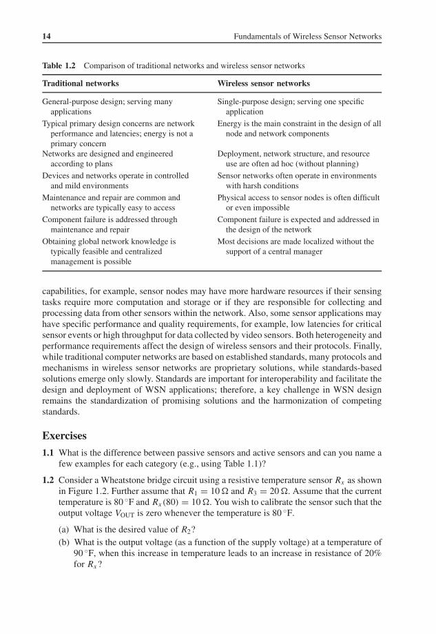
Table 1.2 Comparison of traditional networks and wireless sensor networks
Traditional networks Wireless sensor networks
General-purpose design; serving manyapplications
Single-purpose design; serving one specificapplication
Typical primary design concerns are networkperformance and latencies; energy is not aprimary concern
Energy is the main constraint in the design of allnode and network components
Networks are designed and engineeredaccording to plans
Deployment, network structure, and resourceuse are often ad hoc (without planning)
Devices and networks operate in controlledand mild environments
Sensor networks often operate in environmentswith harsh conditions
Maintenance and repair are common andnetworks are typically easy to access
Physical access to sensor nodes is often difficultor even impossible
Component failure is addressed throughmaintenance and repair
Component failure is expected and addressed inthe design of the network
Obtaining global network knowledge istypically feasible and centralizedmanagement is possible
Most decisions are made localized without thesupport of a central manager
capabilities, for example, sensor nodes may have more hardware resources if their sensingtasks require more computation and storage or if they are responsible for collecting andprocessing data from other sensors within the network. Also, some sensor applications mayhave specific performance and quality requirements, for example, low latencies for criticalsensor events or high throughput for data collected by video sensors. Both heterogeneity andperformance requirements affect the design of wireless sensors and their protocols. Finally,while traditional computer networks are based on established standards, many protocols andmechanisms in wireless sensor networks are proprietary solutions, while standards-basedsolutions emerge only slowly. Standards are important for interoperability and facilitate thedesign and deployment of WSN applications; therefore, a key challenge in WSN designremains the standardization of promising solutions and the harmonization of competingstandards.
Exercises
1.1 What is the difference between passive sensors and active sensors and can you name afew examples for each category (e.g., using Table 1.1)?
1.2 Consider a Wheatstone bridge circuit using a resistive temperature sensor Rx as shownin Figure 1.2. Further assume that R1 = 10 � and R3 = 20 �. Assume that the currenttemperature is 80 ◦F and Rx(80) = 10 �. You wish to calibrate the sensor such that theoutput voltage VOUT is zero whenever the temperature is 80 ◦F.
(a) What is the desired value of R2?(b) What is the output voltage (as a function of the supply voltage) at a temperature of
90 ◦F, when this increase in temperature leads to an increase in resistance of 20%for Rx?

Motivation for a Network of Wireless Sensor Nodes 15
1.3 As described in this chapter, using multiple communication hops instead of a single hopaffects the overall energy consumption. Describe other advantages or disadvantages ofmulti-hop communications, for example, in terms of performance (latency, throughput),reliability, and security.
1.4 The relationship between the transmitted and the received power of an RF signal fol-lows the inverse-square law shown in Equation (1.5), that is, power density and distancehave a quadratic relationship. This can be used to justify multi-hop communication(instead of single-hop), that is, energy can be preserved by transmitting packets overmultiple hops at lower transmission power. Assume that a packet p must be sent froma sender A to a receiver B. The energy necessary to directly transmit the packet canbe expressed as the simplified formula EAB = d(A, B)2 + c, where d(x, y) (or sim-ply d in the remainder of this question) is the distance between two nodes x and y
and c is a constant energy cost. Assume that you can turn this single-hop scenariointo a multi-hop scenario by placing any number of equidistant relay nodes betweenA and B.
(a) Derive a formula to compute the required energy as a function of d and n, where n
is the number of relay nodes (that is, n = 0 for the single-hop case).(b) What is the optimal number of relay nodes to send p with the minimum amount
of energy required and how much energy is consumed in this optimal case for adistance d(A, B) = 10 and (i) c = 10 and (ii) c = 5?
1.5 Name at least four techniques to reduce power consumption in wireless sensor networks.
ReferencesBult, K., Burstein, A., Chang, D., Dong, M., Fielding, M., Kruglick, E., Ho, J., Lin, F., Lin, T.H., Kaiser, W.J.,
Marcy, H., Mukai, R., Nelson, P., Newburg, F.L., Pister, K.S.J., Pottie, G., Sanchez, H., Sohrabi, K., Stafsudd,O.M., Tan, K.B., Yung, G., Xue, S., and Yao, J. (1996) Low power systems for wireless microsensors. Proc.of the International Symposium on Low Power Electronics and Design .
Calhoun, B.H., Daly, D.C., Verma, N., Finchelstein, D.F., Wentzloff, D.D., Wang, A., Cho, S.H., and Chan-drakasan, A.P. (2005) Design considerations for ultralow energy wireless microsensor nodes. IEEE Trans-actions on Computers 54 (6), 727–749.
Cerpa, A., and Estrin, D. (2004) Ascent: Adaptive self-configuring sensor network topologies. IEEE Transactionson Mobile Computing 3 (3), 272–285.
DAR (1978) Proceedings of the Distributed Sensor Nets Workshop. Pittsburgh, PA, Department of ComputerScience, Carnegie Mellon University.
De, V., and Borkar, S. (1999) Technology and design challenges for low power and high performance. Proc. ofthe International Symposium on Low Power Electronics and Design (ISLPED).
Gutierrez, J.A., Naeve, M., Callaway, E., Bourgeois, M., Mitter, V., and Heile, B. (2001) IEEE 802.15.4: A devel-oping standard for low-power low-cost wireless personal area networks. IEEE Network 15 (5), 12–19.
Kahn, J.M., Katz, R.H., and Pister, K.S.J. (1999) Mobile networking for smart dust. Proc. of the ACM/IEEEInternational Conference on Mobile Computing and Networking (MobiCom).
Mills, K.L. (2007) A brief survey of self-organization in wireless sensor networks. Wireless Communications andMobile Computing 7 (7), 823–834.
Pottie, G.J. (2001) Wireless integrated network sensors (WINS): The web gets physical. National Academy ofEngineering: The Bridge 31 (4), 22–27.
Pottie, G.J., and Kaiser, W.J. (2000) Wireless integrated network sensors. Communications of the ACM .Rabaey, J., Ammer, J., da Silva, Jr J.L., and Patel, D. (2000) Picoradio: Ad hoc wireless networking of ubiquitous
low-energy sensor/monitor nodes. Proc. of the IEEE Computer Society Annual Workshop on VLSI.

16 Fundamentals of Wireless Sensor Networks
Shih, E., Bahl, P., and Sinclair, M. (2002) Wake-on wireless: An event driven energy saving strategy for batteryoperated devices. Proc. of the ACM/IEEE International Conference on Mobile Computing and Networking(MobiCom).
Shih, E., Cho, S.H., Ickes, N., Min, R., Sinha, A., Wang, A., and Chandrakasan, A. (2001) Physical layer drivenprotocol and algorithm design for energy-efficient wireless sensor networks. Proc. of the 7th Annual Interna-tional Conference on Mobile Computing and Networking .
Sinha, A., and Chandrakasan, A.P. (2000) Energy aware software. Proc. of the 13th International Conference onVLSI Design .
Sohrabi, K., Gao, J., Ailawadhi V., and Pottie, G. (2000) Protocols for self-organization of a wireless sensornetwork. IEEE Personal Communications Magazine 7 (5), 16–27.
Ye, W., Heidemann, J., and Estrin, D. (2004) Medium access control with coordinated adaptive sleeping for wire-less sensor networks. IEEE/ACM Transactions on Networking 12 (3), 493–506.

2ApplicationsWireless sensor networks have inspired many applications. Some of them are futuristicwhile a large number of them are practically useful. The diversity of applications in thelatter category is remarkable – environment monitoring, target tracking, pipeline (water,oil, gas) monitoring, structural health monitoring, precision agriculture, health care, supplychain management, active volcano monitoring, transportation, human activity monitoring,and underground mining, to name a few. In this chapter some of these applications and theprototype implementations for these applications will be discussed in some detail.
2.1 Structural Health Monitoring
On 2 August 2007, a highway bridge unexpectedly collapsed in Minnesota into the fast-flowing Mississippi river. Nine people were killed in the event. The National TransportationSafety Board investigators were unable to determine the cause of the accident, but theyshort-listed three potential causes, namely, wear and tear, weather, and the weight of a nearbyconstruction project which was taking place at the time. The construction project was closinghalf of the bridge’s eight lanes when the accident happened. Two weeks later – on 14 August2007 – another bridge collapsed at a popular Chinese tourist spot in Fenghuang county inHunan province, killing 86 people on the spot. In fact, the BBC reported (14 August 2007)that China had identified more than 6000 bridges that were damaged or considered to bedangerous.
During and following these accidents, several news outlets, including The AssociatedPress (3 August 2007) and Time magazine (10 August 2007), featured articles that advocatedwireless sensor networks for monitoring bridges and similar structures.
Traditionally, bridges are inspected in different phases and at different levels (Koh andDyke 2007):
1. visual inspection carried out by road maintenance crews during routine road inspections,normally every day;
2. basic inspections carried out usually at least once a year by local bridge inspectors;3. detailed inspection, carried out at least every five years on selected bridges by regional
bridge inspectors; and4. special inspections carried out by highly qualified experts and researchers according to
technical needs, normally as a consequence of questionable results from basic or detailedinspections.
Fundamentals of Wireless Sensor Networks: Theory and Practice Waltenegus Dargie and Christian Poellabauer 2010 John Wiley & Sons, Ltd

18 Fundamentals of Wireless Sensor Networks
The first phase is a labor-intensive, tedious, inconsistent, and subjective inspectiontechnique (Koh and Dyke 2007), whereas the rest require sophisticated tools, whichare usually expensive, bulky, and power consuming. Subsequently, developing auto-mated, efficient, and affordable structural health monitoring techniques is an activeresearch area.
Broadly speaking, tool-based inspection techniques can be classified into local andglobal inspections (Chintalapudi et al. 2006). Local techniques focus on detecting highlylocalized, imperceptible fractures in a structure. These techniques employ ultrasonic,thermal, X-ray, magnetic or optical imaging techniques, but this type of inspectionrequires a significant amount of time and the disruption of the normal operation of thestructure.
Global inspection techniques, on the other hand, aim to detect a damage or defectthat is large enough to affect the entire structure. Often this is carried out by detectingconspicuous changes in the movements of abutments, balustrades and barriers, bridgebearings, decks, towers, expansion joints, railings, etc., to forced or ambient excitations.Global inspection techniques can be considered as an inverse problem, that is, the statusof the structure is determined on the basis of its response to an external excitation. Theexcitation can be ambient (such as an earthquake or a strong wind) or forced (such asa deliberate force produced by a shaker or an impact hammer). In either case, modalparameters, such as natural frequencies, damping ratios, and mode shapes are investigatedto identify damage in the form of expansion, de-lamination, corrosion, debonding,cracking, etc.
Modal parameters are determined by several factors including: the magnitude and dura-tion of the excitation; the material from which the structure is made; the size of the structure;the technical restrictions in the construction; the age of the structure; and other surroundingconstraints.
More recently, researchers have been developing and testing wireless sensor networks aspart of a global inspection mechanism. There are three aspects that make them suitable forthe task:
1. The sensor nodes can be placed in areas that are inaccessible to wired and bulkydevices.
2. By deploying a large number of nodes, it is possible to establish correlation betweendifferent measurements. This facilitates localizing damage.
3. Ideally, the deployment as well as the management (maintenance) of the sensor networkdoes not require disruption of the normal operation of the structure.
2.1.1 Sensing Seismic Events
Seismic responses in large structures are transient by nature and comprise frequencies belowa few tens of hertz. The response can be captured by employing acceleration sensors, tiltsensors, and piezoelectric sensors. However, the sensors should be oversampled at highfrequency to compensate for noise and imperfect placement.
Some of the challenges pertaining to the analysis of data are: (a) restrictions regardingthe characteristics of the excitations; (b) the presence of unreachable degree-of-freedom

Applications 19
elements; (c) measurement noise; (d) modeling errors; and (e) environmental constraints.The effectiveness of a technique is measured by its capability to extract a sufficiently largeamount of damage-sensitive parameters (stiffness, damping, etc.), given limited and incom-plete modal data measured from a real structure.
A damage detection technique can identify a single damage or multiple damages, depend-ing on the model of the structure. Single-damage detection usually employs natural frequen-cies while the multiple damage detection technique employs mode shapes.
2.1.2 Single Damage Detection Using Natural Frequencies
This technique computes the correlation between the measured and predicted (hypothesis)modal frequencies to determine the damage. The parameter vectors used for evaluatingcorrelation coefficients consist of the ratio of the first n modal frequency changes due toa damage in the structure, that is, �ω = (ωh − ωd), where ωh and ωd denote the naturalfrequency vectors of the healthy and damaged elements of the structure, respectively. Thehypothesis vector, predicted from an analytic model, is used to infer the location and extentof damage. It is denoted by δω.
Given a pair of parameter vectors, one can estimate the level of correlation in severalways. The simplest way of estimating correlation is to calculate the angle between ωh andωd . A damage localization technique using the pair comparison attempts to find linear cor-relation of modal frequency variation vectors. One way is to apply Equation (2.1) (Koh andDyke 2007):
Cj = �ωT δωj
|�ω||δωj | (2.1)
where the subscript j = (1, 2, ..., r) indicates the hypothesized location of the damage.Another possibility is to apply the damage localization assurance criterion, or in short,
DLAC, which is expressed as:
DLACj =∣∣�ωT δωj
∣∣2(�ωT �ωj )(δω
Tj δωj )
(2.2)
Equation (2.2), similar to Equation (2.1), compares two frequency change vectors(namely, one based on the measurement obtained from the test structure and the other basedon the j th hypothesis of an analytical model of the structure) in order to evaluate the levelof correlation between the two parameter vectors.
2.1.3 Multiple Damage Detection Using Natural Frequencies
Damage inference based on a unique pattern in modal frequency changes yields erroneousresults when applied to a structure with a multiple or unknown number of defects. Incor-porating a sensitivity matrix derived from the analytic model of the structure into Equation(2.1) enables multiple damages to be estimated. The sensitivity matrix consists of the first-order derivatives of the modal frequencies with respect to each foreseeable damage variable,

20 Fundamentals of Wireless Sensor Networks
for the ratio of stiffness reduction in each structural element. This is given as (Koh and Dyke2007):
S =
∂ω1
∂z1
∂ω1
∂z2· · · ∂ω1
∂zn∂ω2
∂z1
∂ω2
∂z2· · · ∂ω2
∂zn...
... · · · ...
∂ωm
∂z1
∂ωm
∂z2· · · ∂ωm
∂zn
(2.3)
where Zi, i = 1, 2, ..., n is a damage variable.Consequently, given δω = Sδz, the multiple damage location assurance criterion
(MDLAC) is given as:
MDLACj =∣∣�ωT
[Sδzj
]∣∣2(�ωT .�ωj
).([
Sδzj
]T.[Sδzj
]) (2.4)
2.1.4 Multiple Damage Detection Using Mode Shapes
The problem with Equation (2.4) lies in evaluating all possible combinations of damage vari-ables that maximize the MDLAC. Efficient search algorithms, such as genetic algorithms,can be applied to determine the correct set of damage variables, but this can only be madeat the cost of computational complexity.
Multiple damage detection techniques, which use mode shapes instead of natural fre-quency changes, can avoid the sensitivity matrix thereby bypassing the need to apply searchalgorithms. There are two types of approach as far as evaluating mode shapes are concerned:
1. The modal assurance criteria (MAC) is determined between paired modes, namely,healthy and damaged. Thus, the number of available MAC values equals the number ofmeasured modes.
2. Instead of individually evaluating the modal assurance criterion value for each modeshape, a single vector of stacked mode shapes can be used for evaluating linearcorrelation.
In both cases, unlike natural frequencies, mode shapes retain spatial information for agiven degree of freedom, that is, correlation between stacked mode shapes can directly indi-cate a damaged location. On the other hand, mode-based correlation techniques can onlyweakly capture the extent of the damage.
The relative change in each mode shape between healthy and damaged states can be usedto calculate the correlation coefficients. The change of mode shapes �(m × r) due to dam-age is transformed into a single vector, vec [��](mr × 1) by stacking r columns of damagesof the matrix ��. Hence, the stack mode shape correlation (SMSC) is:
SMSCj = vec [��]T vec[δ�j
]∣∣vec [��]T vec
[δ�j
]∣∣ (2.5)
where vec [��] and vec [δ�] represent stacked vectors for the variation of the identifiedand predicted mode shapes, respectively.

Applications 21
2.1.5 Coherence
Another approach to damage detection and localization is by the use of the coherence func-tion. The coherence, Cxy(ω), between two time discrete signals, x[n] and y[n], 0 ≤ n ≤ ∞,is the normalized function of the frequency derived from the cross-spectrum of the twosignals:
Cxy(ω) = Sxy
SxxSyy
(2.6)
The coherence function measures the extent to which the two signals are linearly relatedwith each other at each frequency. A unity value indicates that the signals are highly cor-related at a given frequency and zero indicates that the signals are uncorrelated at thatfrequency. Coherence is a complex quantity, but it is often approximated by the magnitudesquared coherence (MSC):
∣∣γxy(w)∣∣2 =
∣∣Sxy(w)∣∣2
Sxx(w) · Syy(w)(2.7)
If the two signals are identical, then the coherence gives a unity result for all frequencies.Similarly, if two signals describe completely uncorrelated random processes, the coher-ence will be zero for all frequencies. For example, a repeated measurement of the seismicresponse of a healthy structure would exhibit a high coherence (near 1) for most frequencies,whereas the coherence of a seismic response of a damaged structure and a healthy structurewould have low coherence (near 0).
Equation (2.7) would always result in a unity magnitude for all frequencies (thoughthe imaginary component may not be 1) if a single window were used to estimate thespectral density. A commonly used multiple windowing method is called weightedoverlapped segment averaging (WOSA) and involves splitting two signals, X and Y,into equal lengths of windowed segments. The Fast Fourier Transform (FFT) of thesesegments is taken and their results are averaged together to estimate the spectral density.The segments can be overlapped to reduce the variance of the spectral estimate (anoverlap of 50% is common). However, overlapping is computationally expensive. Ingeneral, more windows provide smoother coherences with less variability but require morecomputation.
Measuring the degree of coherence of two signals at each potential frequency requiresthat the signals are well represented at each frequency, that is, the power of the signals ateach frequency should be appreciably large enough and the two signals should be well syn-chronized. This requires precise sensors, narrow-band filters to isolate the desired frequencycomponents from higher harmonics, and sampling the signals at high rate. Therefore, insteadof evaluating coherence at each frequency, one can integrate the area under the coherencecurve for a given frequency range. Domain knowledge of the structural response can betaken into account to limit the range. For large bridges, for example, the range lies below10 Hz. Subsequently, a normalized integration over the range 0 to 10 Hz to get a 0 to 1measure of the coherence can be achieved:
Pxy = 1
10
∫ 10
0Cxy(ω)dω (2.8)

22 Fundamentals of Wireless Sensor Networks
2.1.6 Piezoelectric Effect
So far the inputs of damage detection techniques are implicitly assumed to be obtainedfrom acceleration sensors or tilt sensors. It is relatively simple to capture seismic responseby employing acceleration sensors. It is also possible to employ piezoelectric materials tocapture a seismic response. When a mechanical stress is applied to a piezoelectric mate-rial, it generates an electric charge; and when an electric field is applied to a piezoelectricmaterial, its dimensions change proportionally to the applied field. This property makes apiezoelectric material suitable for seismic sensing or actuation, or both.
The relation between the mechanical and electrical variables associated with a piezoelec-tric material can be described as follows (Park et al . 2000):
Si = SEij Tj + dmiEm (2.9)
Dm = dmiTi + εTmk (2.10)
This can be reformulated as: [S
D
]=[
sE dt
d εT
] [T
E
](2.11)
In Equations (2.9)–(2.11), the parameters are defined as follows:
• S is the mechanical strain;• T is the mechanical stress;• E is the electric field;• D is the charge density;• s is the mechanical compliance;• d is the piezoelectric strain constant;• ε is the permittivity; and• the subscripts i, j, m, and k indicate the direction of stress, strain, or electric field.
C
Y = Re{Y} + j Im{Y}
I = i sin(wt + f)
MPZT
R
V = v sin(wt)
Figure 2.1 A piezoelectric material for capturing mechanical impedance. The PZT is normallybonded directly to the surface of the structure by a high strength adhesive to ensure better mechanicalinteraction - this is indicated by the gray box, M. The broken line indicates the coupled electrome-chanical admittance Y (Park et al 2000).

Applications 23
Equation (2.9) describes the change in the dimension of a piezoelectric material as aresult of an applied electric field, whereas Equation (2.10) describes the electric field that isinduced by piezoelectric material in response to an applied mechanical stress.
Equation (2.10) is important for structural health monitoring, because it quantitativelydescribes the variation in the mechanical impedance due to the presence of structural dam-age. More precisely, it means that by employing a piezoelectric material, it is possibleto couple the mechanical and electrical impedance thereby extracting structural informa-tion from electrical impedance measurements. Mathematically, the relationship between themechanical impedance and the electrical impedance is described as:
Y (ω) = jωwala
ha
(εT
33(1 − jδ) − Zs(ω)
Zs(ω)Za(ω)d2
3xYExx
)(2.12)
where
• Y is the electrical admittance;• Za is the mechanical impedance of the piezoelectric material;• Zs is the mechanical impedance of the structure;• Yxx is Young’s modulus of piezoelectric material at zero electric field (inverse of
compliance);• d3x is the piezoelectric strain constant at zero stress;• εT
33 is the permittivity at zero stress;• d is the dielectric loss tangent to the piezoelectric material; and• wa is the width, la is the length, and ha is the thickness of the piezoelectric material,
respectively.
The electrical admittance is the inverse of impedance, Z, in electrical engineering. Theimpedance, Z, can have a resistive, an inductive, or a capacitive component, or a combina-tion of these. If the material is a simple resistor, the impedance is equal to the resistance ofthe material, R, which can be simplified as:
R = v(t)
i(t)(2.13)
where v(t) is a timely varying potential difference measured at the two ends of the resistorand i(t) is a timely varying current flowing through the resistor. R is real, which meansthat the current is in phase with the voltage. If the material is a pure coil, with no resistivecomponent, the impedance, Z, is expressed as:
Z(ω) = v(t)
i(t)= jωL (2.14)
where L is the inductance of the material and ω = 2πf is the angular velocity, signifyingthe rate of change of the potential difference, v(t). j implies that the voltage and thecurrent are out of phase by 90◦ as a result of the inductive effect. A positive j indicatesthat the current is leading the voltage. The inductance, L, of the material depends onthe length of the conductor, the number of coils, and the conductivity of the conductor.In reality no coil is purely inductive, it will have some resistive component, R. Hence,

24 Fundamentals of Wireless Sensor Networks
for a real coil with a resistive component, the impedance, Z, of Equation (2.14) ismodified to:
Z(ω) = v(t)
i(t)= R + jωL (2.15)
If the material is capacitive (if two conductors are separated by a dielectric material andthere is a potential difference between the two conductors), the impedance of the materialis given as:
Z(ω) = v(t)
i(t)= 1
jωC(2.16)
where C is the capacitance of the material; and j indicates that the voltage and the currentare out of phase by 90◦, the voltage leading the current.
The capacitance of a material, C, depends on the cross-sectional area of the two conduc-tors, the distance of separation, and the dielectric material that separates them. In general, theimpedance through which an electric charge is flowing as a result of the potential differencev between the two ends of the material is given as:
Z(ω) = v(t)
i(t)= R + jωL
jωC(2.17)
With this in mind, if the impedance of the piezoelectric material and the magnitude andfrequency of the electric field induced inside the piezoelectric material are known, it is pos-sible to determine the mechanical stress in Equation (2.12). Figure 2.1 demonstrates thetransformation of mechanical admittance to an electrical admittance through the employ-ment of a piezoelectric material.
Accordingly:
Zs(ω) = Za(ω)
εT33(1 − jδ) − Y (ω)ha
jωwala
(d3x)2YE
xx − εT33(1 − jδ) + Y (ω)ha
jωwala
(2.18)
Equation (2.18) illustrates that the mechanical impedance of a structure can be deter-mined from the electrical admittance of the piezoelectric bonding. In other words, struc-tural integrity can be evaluated by measuring the electrical impedance of the piezoelectricsensor.
2.1.7 Prototypes
Wisden is the first prototype to employ wireless sensor networks for monitoring structuralhealth. It is developed at the University of Southern California and deployed (a) on a seismictest structure and (b) in an abandoned, four-story office building in Los Angeles (a victim ofthe 1994 Northridge earthquake). The seismic test structure used as a platform for conduct-ing seismic experiments is an imitation of a full-scale 28 × 28 ft2 hospital ceiling. It supports10,000 lb of weight and can be subjected to a uniaxial motion of a peak-to-peak stroke of

Applications 25
10 in. with a 55,000-lb hydraulic actuator with a ±5-in. stroke. The hydraulic pump deliversup to 40 gallons per minute at 3000 lb/in2. The overall weight of the moving portion of thetest structure is approximately 12,000 lb.
The Wisden sensor network (Xu et al. 2004; Chintalapudi et al. 2006) consists of 25nodes and a 16-bit vibration card, which is specifically designed for high-quality, low-power vibration sensing. A high-sensitive triaxial accelerometer is attached to the vibrationcard.
The nodes organize themselves to establish a tree topology WSN. The topology of the net-work is dynamically adjusted to accommodate incoming nodes and the departure of existingones (due, for example, to the failure or exhaustion of batteries). The task of the network isto reliably send time-synchronized vibration data to a remote sink over a multi-hop route.To ensure reliable transmission, Wisden implements a negative acknowledgment (NACK),hybrid hop-by-hop/end-to-end transmission scheme. The hop-by-hop scheme enables inter-mediate nodes to identify and retransmit lost messages by observing gaps between receivedsequence numbers. For this reason, every node stores transmitted messages in a messagecache. Wisden ensures reliable transmission of sensed data in the presence of up to 30%loss rate.
Another prototype was developed at the University of California, Berkeley, and deployedat the Golden Gate Bridge in San Francisco (Kim et al. 2007). The bridge has a centerspan that sustains a maximum transverse deflection (due to wind or earthquake) of27.7 ft and maximum upward and downward deflections of 5.8 ft and 10.8 ft, respectively.The towers are 500 ft high above the roadway and 746 ft high above the water. Thetops of the towers can have transverse deflections of up to 12.5 in. and toward the shorelongitudinal deflections of 22 in. Sixty-four wireless sensor nodes were deployed on this
(b)
(a)
30 nodes
10 nodes
10 nodes
Figure 2.2 The deployment scenario of on the Golden Gate Bridge. (a) The nodes are deployed onboth side of the span. (b) A two-dimensional view of the placement of nodes on the bridge.

26 Fundamentals of Wireless Sensor Networks
bridge to establish a structural health monitoring network. The nodes were distributedover the main span and the tower, collecting ambient vibrations synchronously, at a rateof 1 kHz, with less than 10 µs jitter and with an accuracy of 30 µG. Data is collectedreliably over a 46-hop network. Figure 2.2 illustrates the deployment at the GoldenGate Bridge.
The goal of the deployment was to determine the response of the structure to bothambient and extreme conditions and to compare actual performance with design predic-tions. The network measured ambient structural accelerations from wind load at closelyspaced locations. It also measured strong shaking from a potential earthquake. Theinstallation as well as the monitoring, was conducted without disrupting the operation of thebridge.
2.2 Traffic Control
Ground transportation is a vital and complex socioeconomic infrastructure. Operationally, itis linked with and provides support for a variety of systems, such as supply-chain, emergencyresponse, and public health. In urban areas, this results in potential congestion. The 2009Urban Mobility Report, issued by the Texas Transportation Institute, reveals that in 2007,congestion caused urban Americans to travel 4.2 billion hours more and to purchase an extra2.8 billion gallons of fuel. The total congestion cost is estimated to be $87.2 billion – anincrease of more than 50% over the previous decade.
Unfortunately, building new roads is not a feasible solution for many cities of the worldowing to the lack of free space and the high cost of demolition of old roads (streets). Manyconsider better regulation of transportation systems as the only sustainable solution to roadcongestion.
One approach to dealing with congestions is to put in place distributed sensing systemsthat reduce congestion. These systems gather information about the density, sizes, and speedof vehicles on roads; infer congestions; and suggest to drivers some alternative routes andemergency exits.
2.2.1 The Sensing Task
A large number of devices are used in traffic control systems. These include video, sonar,radar, inductive loops, magnetometers, microloop probes, pneumatic road tubes, piezoelec-tric cables, PVDF wire, and pneumatic treadle. Video and sonar-based sensing systems needto be installed on poles, while inductive loops, magnetometers, and pneumatic treadles canbe embedded into the transportation infrastructure. Camera-based systems involve humanoperators to process images, identify incidents, and assign speed rankings. Apparently, thistechnique is costly and can only be employed in selected streets, such as those that arefrequently traveled.
Another way is to fully automate congestion recognition. There are several approachesto do this. For example, automated camera-based systems use machine vision to count andclassify vehicles. Alternatively, they target the license numbers of passing vehicles and asso-ciate driving history as a means of estimating congestion causes. These approaches are wellsuited as long as the data from the cameras is reliable. In the presence of fog, smog, dust,snow, or rain, however, roadside cameras are unreliable.

Applications 27
2.2.1.1 Inductive Loops
More recently, in-road sensing devices have been developed as complementary systems.These devices are interesting because they are unaffected by weather and provide directinformation with very little ambiguity. One of the most common in-road traffic sensors isthe inductive loop (Knaian 2000). This is a coil of wire several meters in diameter and can beburied under the road and connected to a roadside control box that passes an electric currentthrough the coil. By establishing relationship between the current, the magnetic field strengththat is induced as a result of the current, and the speed and size of the passing vehicles, it ispossible to infer traffic flow. The exact relationship between the current and a vehicle canbe defined by using Faraday’s induction law.
According to Faraday’s law, when an electric current passes through a conductor, it pro-duces a magnetic field around the conductor. The direction of the field is normal to thedirection of the current flow. The strength and density of the magnetic field depends on thelength and cross-sectional area of the conductor as well as the material from which the con-ductor is made, that is, the permeability of the conductor, µ. The ratio of the magnetic flux,�, to the current is called inductance, L, which is defined as:
L = �
i(2.19)
If, instead of a straight conductor, the current passes through a solenoid (a long, thincoil, with a length much greater than the diameter of the loop) of N turns and length l, themagnetic flux density, B, induced in it is expressed as:
B = µ0Ni
l(2.20)
where µ0 is the permeability of free space; N is the number of turns; i is the current; and l
is the length of the coil. The magnetic flux through the coil is obtained by multiplying theflux density B by the cross-sectional area, A and the number of turns, N :
� = µ0N2i
A
l(2.21)
Reformulating Equation (2.21) will yield:
L = µ0N2 A
l(2.22)
The inductance of a solenoid changes when vehicles drive on the road, disturbing theinduced magnetic flux. The magnitude of the change depends on the vehicle’s speed andsize. To determine the speed of the vehicle, two loops separated by a distance, d , of knownlength are sufficient.
Measuring the change in voltage or current is easier than measuring the change in mag-netic field strength or magnetic flux. The induced electromotive force in a closed loop isdirectly proportional to the rate of change of magnetic flux through the loop. This can bebetter explained by moving a conductor through a magnetic field, which induces a voltagein that conductor. The induced voltage is proportional to the speed of movement, the lengthand cross-sectional area of the conductor, and the strength of the magnetic field. If the con-ductor forms a solenoid, the number of turns of the conductor influences the induced voltage.

28 Fundamentals of Wireless Sensor Networks
The magnetic field, the direction of movement, and the voltage are all orthogonal to eachother. To determine their exact direction, Fleming’s right-hand rule can be applied. Alter-natively, it is also possible to keep the conductor stationary and vary the magnitude anddirection of the magnetic field to induce a voltage in a conductor. Mathematically, this isexpressed as:
ε = −Nd�B
dt(2.23)
where ε is the electromotive force (emf) in volts; N is the number of turns of wire; �B isthe magnetic flux in Weber that passes through a single loop. The negative sign in Equation(2.23) indicates that the direction of the electromotive force is opposite to the direction of themagnetic flux. The magnetic flux is a function of the cross-sectional area of the conductorand the magnetic field strength, which is normal to the conductor. Lenz’s law can be appliedto determine the direction of the induced electromotive force (emf) and current resultingfrom electromagnetic induction.
d�
dt= A dB
dt(2.24)
More generally, the relation between the rate of change of the magnetic flux through asurface S enclosed by a contour C and the electric field along the contour is expressed as:∮
C
E · dl = − d
dt
∫S
B · dA (2.25)
where E is the electric field; dl is an infinitesimal element of the contour C; and B is themagnetic field strength. The directions of the contour C and dA are assumed to be relatedby the right-hand rule.
Equivalently, the differential form of Faraday’s law can be employed:
∇ × E = −∂B∂t
(2.26)
The only limitation of inductive loops is their physical size. First, deployment requiresthe complete dismantlement of an entire cross-section of a road. Second, it is difficult todistinguish vehicles in bumper-to-bumper traffic, since two vehicles may cross the loop atthe same time.
2.2.1.2 Magnetic Sensors
The presence, direction, and speed of a vehicle can be determined by employing magneticsensors. The technique requires a magnetic field of known strength and direction. A movingvehicle can disturb the distribution of the magnetic field either by producing its own mag-netic field or simply by cutting across it. As the magnitude and direction of the disturbancedepends on the speed, size, density, and permeability of the vehicle, it is possible to usemagnetic sensors to quantify the disturbance.
Magnetic sensors can be classified into low-field, medium-field, and high-field sensors,according to the range of the strength of the magnetic field they measure (Caruso andWithanawasam 1999). Low-field sensors measure magnetic field strength below 1 µG

Applications 29
(micro Gauss); medium-field sensors measure between 1 µG and 10 G; high-field sensorscan measure above 10 G. The Earth’s magnetic field is found in the medium field.
Magnetic fields are set up by the motion of electrical charges. For instance, the mag-netic field of a bar magnet is created by the motion of negatively charged electrons withiniron atoms. The cause of the Earth’s magnetic field is not completely understood, but it isbelieved to be associated with electrical currents produced by the coupling of convectiveeffects and rotations in the spinning liquid metallic outer core of iron and nickel. It has auniform distribution over a wide area (several kilometers). It was first measured by CarlFriedrich Gauss in 1835 and has been repeatedly measured since then, showing a relativedecay of about 5% over the last 150 years.
Sensors that can measure the Earth’s magnetic field comprise an alloy of nickel and iron.Typical examples are anisotropic magnetoresistive (AMR) sensors whose resistive propertychanges according to the Earth’s magnetic field strength. AMR sensors can measure bothlinear and angular positions and displacement in the Earth’s magnetic field.
Almost all road vehicles, including those with polymer body panels, contain a large massof steel. Since the magnetic permeability of steel is much higher than the surrounding air, ithas the capacity to concentrate the flux lines of the Earth’s magnetic field. The concentrationof magnetic flux (disturbance) at a particular location varies as the vehicle moves and canbe detected from a distance of up to 15 m (Weaver 2003). Figure 2.3 demonstrates how anAMR sensor can be used to measure the disturbance in the Earth’s magnetic field caused bya moving vehicle.
It is possible to distinguish between different types of vehicles (car, bus, minibus, truck,etc.) by modeling a vehicle as a composition of many dipole magnets (Caruso and With-anawasam 1999). These dipoles have north–south orientations that cause distortions inthe Earth’s magnetic field. The extent of the distortions of the dipoles depends on, amongother things, the permeability of the dipoles. For example, the engine and wheel areas exertstronger distortions than the other parts of a vehicle, and for each vehicle class of interest,it is possible to produce a unique model. When a vehicle passes close to a magnetic sensor,or drives over it, the sensor can detect the different dipole moments of the various parts ofthe vehicle. The field variation reveals a detailed magnetic signature.
Figure 2.3 Detection of a moving vehicle with an AMR magnetic sensor (Caruso and With-anawasam 1999).

30 Fundamentals of Wireless Sensor Networks
2.2.2 Prototypes
Knaian (2000) proposes the use of wireless sensor networks for traffic monitoring in urbanareas. A prototype was deployed in Vassar Street, Cambridge, Massachusetts. The wirelesssensor node consists of two AMR magnetic sensors for detecting vehicular activities and atemperature sensor for monitoring road condition (snow, ice, or water). The movement andspeed of a vehicle is captured by observing the disturbance it creates in the Earth’s magneticfield. This takes the form of an excursion first below and then above a predefined baseline,since the vehicle pulls field lines away from the sensor when it approaches it and then towardthe sensor when it drives away from it.
To measure the speed of a vehicle, the node waits until it detects an excursion from thebaseline and then starts sampling at a frequency of 2 kHz. An AMR magnetic sensor isplaced at the front of the node and another at the back. The waveforms at the outputs of thesensors are identical, except that they are shifted in time and may be affected by noise. Whenthe signal from the rear sensor crosses the baseline, the node begins to count the number ofsamples until the signal from the forward sensor crosses the baseline. From this count, itcomputes the speed of the passing vehicle.
In order to detect a vehicle during bumper-to-bumper drive, a minimum of three samplesat a frequency of 100 Hz are required for the following vehicle description: average drivespeed is 40 mph (or 20 meters per second) and the size of the engine block is 60 cm. In otherwords, the sampling frequency fs should be:
fs = 20 m/s × 3 × 100
60 cm= 100 Hz (2.27)
Sampling at this rate enables the node to detect vehicles that travel at a higher speed (asfast as 200 mph), with a minimum separation distance of 3 m. Figure 2.4 displays the blockdiagram of the sensor node developed at MIT.
Arora et al. (2004) deployed 90 Mica2 sensor nodes at MacDill Air Force Base in Tampa,Florida, to detect the movement of vehicles, soldiers, and people. Seventy-eight of the nodeswere magnetic sensor nodes that were deployed in a 60 × 25 square foot area. Additionally,12 radar sensor nodes were overlaid on the network. The magnetic sensor nodes were dis-tributed uniformly. These nodes form a self-organizing network which connects itself to aremote computer via a base station and a long-haul radio repeater.
The Mica2 nodes were based on a 4 MHz Atmel processor with 4 kbytes random accessmemory, 128 kbytes of flash program, and 512 kbytes of EEPROM memory (used for datalogging). The TinyOS operating system runs on the nodes. Magnetic fields were sensed byusing an in-built magnetometer while the TWR-ISM-002 radar motion sensor was used todetect movement of objects.
2.3 Health Care
A wide range of health care applications have been proposed for wireless sensor networks,including monitoring patients with Parkinson’s Disease, epilepsy, heart patients, patientsrehabilitating from stroke or heart attack, and elderly people. Unlike other types of appli-cations discussed so far, health care applications do not function as stand-alone systems.Rather, they are integral parts of a comprehensive and complex health and rescue system.

Applications 31
Microcontroller(TMS430)
AMR MagneticSensor
Instrumentationand Operational
Amplifiers
MOSFET
Power
AMR MagneticSensor
Instrumentationand Operational
Amplifiers
MOSFET
Power
Strap Control Radio Transmitter
Antenna
MOSFET
Power
TemperatureSensor
Channel A
Channel B
Figure 2.4 Block diagram of the MIT node for traffic monitoring (Knaian 2000).
According to the US Centers for Medicare and Medicaid Services (CMS), the nationalhealth spending of the country in 2008 was estimated to be $2.4 trillion. The cost of heartdisease and stroke takes around $394 billion. The same report projects a rise in health spend-ing in the US as well as in many western countries. Apparently, this is a concern for policymakers, health care providers, hospitals, insurance companies, and patients.
Interestingly, higher spending does not necessarily correlate with a high quality serviceor prolonged lifetime (Kulkarni and Ozturk 2007). For example, in 2000, the US spent moreon health care than any other country in the world – an average of $4500 per person – butranked 27th in average life expectancy. Many countries achieved higher life expectancyrates at a lower cost.
While preventive health care has been advocated by many as a means to reduce healthspending and mortality rate, studies show that some patients find that certain practicesare inconvenient, complicated, and interfere with their daily life (Morris 2007). For

32 Fundamentals of Wireless Sensor Networks
example, many miss checkup visits or therapy sessions because of a clash of scheduleswith established living and working habits, fear of overexertion, or transportation cost.
To deal with these problems, research attempts to provide a comprehensible solution thatinvolves the following tasks:
• building pervasive systems that provide patients with rich information about diseases andtheir prevention mechanisms;
• seamless integration of health infrastructures with emergency and rescue operations aswell as transportation systems;
• developing reliable and unobtrusive health-monitoring systems that can be worn bypatients to reduce the responsibilities and presence of medical personnel;
• alerting nurses and doctors when medical intervention is necessary; and• reducing inconvenient and costly checkup visits by creating reliable links between
autonomous health-monitoring systems and health institutions.
2.3.1 Available Sensors
The research community has been very active in developing a plethora of wearable and wire-less systems that seamlessly monitor heart rate, oxygen level, blood flow, respiratory rate,muscle activities, movement patterns, body inclination, and oxygen uptake (VO2). Givenbelow is a concise summary of some of the commercially available wireless sensor nodesfor health monitoring:
• pulse oxygen saturation sensors: they measure the percentage of hemoglobin (Hb) satu-rated with oxygen (SpO2) and heart rate (HR);
• blood pressure sensors;• electrocardiogram (ECG);• electromyogram (EMG) for measuring muscle activities;• temperature sensors – both for core body temperature and skin temperature;• respiration sensors;• blood flow sensors;• blood oxygen level sensor (oximeter) for measuring cardiovascular exertion (distress).
2.3.2 Prototypes
2.3.2.1 Artificial Retina
Schwiebert et al. (2001) developed a microsensor array that can be implanted in the eyeas an artificial retina to assist people with visual impairments. The system consists of anintegrated circuit and an array of sensors. The integrated circuit is a multiplexer with on-chipswitches and pads to support a 10 × 10 grid of connections; it operates at 40 kHz. Moreover,it has an embedded transceiver for wired and wireless communications. Each connectionin the chip interfaces a sensor through an aluminum probe surface. Before the bonding isdone, the entire integrated circuit, except the probe areas, is coated with a biologically inertsubstance.

Applications 33
Camera imageprocessing unit
CCD camera(1000 x 1000 image)
Image post processing;data reduction andfeature extraction
Wirelessinterface
Wiredcommunication
Sensing system
DSPPower/data
(RF)transmission
In-vivowirelessreceiver
Retinachip
Neuralinterface
Figure 2.5 The processing components of the artificial retina (Schwiebert et al . 2001).
Each sensor is a microbump. It starts with a rectangular shape, but near the end tapersto a point and rests gently on the retina tissue. The sensors are sufficiently small and lightto be held in place with relatively little force. The distance between adjacent microbumpsis approximately 70 µm. The sensors produce electrical signals proportional to the lightreflected from an object being perceived. The ganglia and additional tissues transform theelectrical energy into chemical energy, which in turn is transformed into optical signals andcommunicated to the brain through the optic nerves. The magnitude and wave shape of thetransformed energy corresponds to the response of a normal retina to light stimulation.
The system is a full duplex system, allowing communication in a reverse direction. Inaddition to the transformation of electrical signals into optical signals, neurological signalsfrom the ganglia can be picked up by the microsensors and transmitted out of the sensingsystem to an external signal processor. In this way, the sensor array is used as a receptionand transmission system in a feedback loop.
Two types of wireless communications are foreseen. First, the eventual mapping of aninput electrical signal to brain patterns cannot be realized internally with the sensing systemalone since signal processing is a computationally intensive process. Second, diagnostic andmaintenance operations require the extraction of data from the sensing system. For thesereasons, interconnecting the sensing system with an external system is essential. In additionto these requirements, communication is required to transfer data from a charge-coupleddevice (CCD) camera (embedded in a pair of spectacles) to the sensor array.
Figure 2.5 illustrates the signal processing steps of the artificial retina. A camera embed-ded in a pair of spectacles directs its output to a real-time digital signal processor (DSP) fordata reduction and processing. The camera can be combined with a laser pointer for auto-matic focusing. The output of the DSP is compressed and transmitted through a wirelesslink to the implanted sensor array, which decodes the image and produces a correspondingelectrical signal.
2.3.2.2 Parkinson’s Disease
Lorincz et al. (2009) and Weaver (2003) propose the use of WSNs to monitor patients withParkinson’s Disease (PD). The aim is to augment or entirely replace a human observer andto help the physician to fine-tune the medication dosage.
34 Fundamentals of Wireless Sensor Networks
Parkinson’s Disease is a degenerative disorder of the central nervous system. It resultsfrom degeneration of neurons in a region of the brain that control movements (substantialnigra), creating a deficiency in neurotransmitter dopamine. Deficiency in dopamine causessevere impairment of motor skills and speech, manifesting itself in tremor of the hands,arms, legs, and jaw; unsteady walk and slowness of movements; and lack of balance andcoordination.
According to the Parkinson’s Disease Foundation (Foundation P.D. 2009), as many asone million Americans live with PD. Approximately 60,000 are diagnosed with the diseaseeach year without considering the thousands of additional cases that go undetected. Thefoundation estimates that 4 million people worldwide are living with PD. The combineddirect and indirect cost of PD, including treatment, social security payments, and lost incomefrom inability to work, is estimated to be nearly $25 billion per year in the United Statesalone.
Persons under treatment (this is usually an external stimulation given to remnant cells inthe substantia nigra to produce more dopamine) can be found in one of the following threephases (Weaver 2003):
1. The exhibition of typical symptoms in the form of tremor and slow movement when thestimulation has worn off. This is known as the off state.
2. Normal movements free of tremor when the medication is balanced. This is known asthe on state.
3. Exaggerated involuntary movements when the medication is at highest concentration.This is known as dyskinesia .
The treatment of PD is case-specific, that is, doctors typically monitor patients on anindividual basis and provide suitable medication to prolong the duration of the on state. Thisrequires a close follow-up of the medication cycle and frequent adjustments. Apparently, thefollow-up is costly. According to the Parkinson’s Disease Foundation, the medication costsfor an individual person are estimated to be $2,500 a year and therapeutic surgery can costup to $100,000 per patient (Foundation P.D. 2009).
Weaver (2003) developed a wearable system that can reduce personnel cost and help aphysician to fine-tune the medication dosage. It consists of a lightweight sensor node with3D accelerometer sensors, a processor core, and a storage system for logging data for laterretrieval. The system could record 17 hours of accelerometer data. The accelerometer sen-sors can be sampled at a rate of 40 Hz.
The system was deployed on PD patients at the Memorial Hospital’s Parkinson Day Cen-ter, Cambridge, MA, and a large amount of data was collected while they performed commondaily tasks (walking, reading quietly while sitting, sitting in animated conversation, etc.).The patients wore the nodes on their ankles and wrists. The report reveals that the systemwas able to identify the occurrence of dyskinesia at the rate of 80%.
More recently, Lorincz et al. (2009) at Harvard University employed a more sophis-ticated wireless sensor node – the Shimmer wireless sensor platform (Sensor platformTSW 2009) – for monitoring patients with PD and epilepsy. The node consists of a TIMSP430 processor, CC2420 IEEE 802.15.4 radio, triaxial accelerometer, and rechargeableLi-polymer battery. It also integrates a MicroSD slot that supports a Flash memory forstoring accelerometer data. This way, the node is capable of storing data from the 3D

Applications 35
accelerometer sensor continuously for more than 80 days at a sampling frequency of50 Hz. In addition to the 3D accelerometer sensor, the node platform provides interfacesfor gyroscope, ECG, EMG, tilt and vibration sensor, and a passive infrared (PIR) motionsensor.
These nodes were deployed on seven patients for one week. Nine nodes were deployedon the body of each patient, two on each arm and leg, and one at the back. Data from 3Daccelerometer sensors and gyroscopes were sampled at a frequency of 100Hz. An initialclinical evaluation was made in various settings, including tuning of deep brain stimulation(DBS) parameters.
2.4 Pipeline Monitoring
Another area of application for wireless sensor networks is the monitoring of gas, water,and oil pipelines. The management of pipelines presents a formidable challenge. Their longlength, high value, high risk, and often difficult access conditions require continuous andunobtrusive monitoring. Leakages can occur due to excessive deformations caused by earth-quakes, landslides, or collisions with an external force; corrosion, wear, material flaws oreven intentional damage to the structure.
To detect leakages, it is vital to understand the characteristics of the substance thepipelines transport. For example, fluid pipelines generate a hot-spot at the location ofthe leak, whereas gas pipelines generate a cold-spot due to the gas pressure relaxation.Likewise, fluid travels at a higher propagation velocity in metal pipelines than in polyvinylchloride (PVC). There are a large number of commercially available sensors (fiber optics,temperature sensors, and acoustic sensors) to detect and localize thermal anomalies.
2.4.1 Prototype
The PipeNet prototype was developed as a collaboration project between Imperial College,London, Intel Research, and MIT to monitor water pipelines in urban areas. Its main taskis to monitor (1) hydraulic and water quality by measuring pressure and pH, and (2) thewater level in combined sewer systems (sewer collectors and combined sewer outflows).Sewerage systems convey domestic sewage, rainwater runoff, and industrial wastewater tosewerage treatment plants. Historically, these systems are designed to discharge their contentto nearby streams and rivers in the event of overflow, such as during periods of heavy rainfall.Subsequently, the combined sewer overflows are among the major sources of water qualityimpairment. Nearly 770 large cities in the US, mainly older communities, have combinedsewer systems (Stoianov et al. 2007).
PipeNet is deployed in three different settings. In the first setting, pressure and pH sensorsare installed on a 12 in. cast-iron pipe which supplies drinking water. Pressure data is col-lected every 5 min for a period of 5 s at a rate of 100 Hz. The wireless sensor node can locallycompute minimum, maximum, average, and standard deviation values and communicate theresults to a remote gateway. Likewise, pH data is collected every 5 min for a period of 10 s ata rate of 100 Hz. The sensor nodes use a Bluetooth transceiver for wireless communication.
The pressure sensor is a modified version of the OEM piezoresistive silicon sensor. It hasan error compensation mechanism to deal with the effects of nonlinearity and hysteresis.The sensor has a startup time of less than 20 ms and a fast dynamic response. It consumesless than 10 mW. The pH sensor is a glass electrode with an Ag/AgCl reference cell.

36 Fundamentals of Wireless Sensor Networks
In the second setting, a pressure sensor is employed to measure the pressure in 8 in. castiron pipe. The data is collected every 5 min for a period of 5 s at a sampling rate of 300 Hz.For this setting, local processing was not supported; instead, the raw data was transmittedto a remote gateway.
Finally, in the third setting, the water level of a combined sewer outflow collector ismonitored. Two pressure transducers were placed at the bottom of the collector and anultrasonic sensor on the top. The pressure sensors are low-power devices and consumeless than 10 mW. The ultrasonic sensor is a high-power device and consumes 550 mW. Forefficient power consumption, the pressure sensors are employed for periodic monitoringwhile the ultrasonic sensor is required only to verify the readings from the pressure sensorswhen their difference exceeded a set threshold or when the water level exceeded the weirheight. In this setting, data collection was carried out at a rate of 100Hz at 5 min intervalsfor a period of 10 s. Moreover, local data aggregation was performed to reduce the net-work traffic. The network supported remote configuration to increase the sampling rate upto 600 Hz.
2.5 Precision Agriculture
Another interesting area where wireless sensor networks motivated a large number ofresearchers is precision agriculture. Traditionally, a large farm is taken as a homogeneousfield in terms of resource distribution and its response to climate change, weeds, and pests.Accordingly, farmers administer fertilizers, pesticides, herbicides, and water resources.In reality, a large field exhibits wide spatial diversity in soil types, nutrient content, andother important factors. Therefore, treating it as a uniform field can cause inefficient use ofresources and loss of productivity.
Precision agriculture is a method of farm management that enables farmers to producemore efficiently through a frugal use of resources. This encompasses different aspects, suchas micro-monitoring soil, crop, and climate change in a field, and providing a decision sup-port system (DSS). Precision agriculture uses Geographic Information System managementtools; GPS, radar, aerial images, etc., to accurately diagnose a field and apply vital farmingresources.
A large number of technologies have been developed over the last several years to facil-itate and automate precision agriculture. Some of these are:
• Yield monitors: These are devices that use, among other things, mass flow sensors, mois-ture sensors, and a GPS receiver to monitor instantaneous yield based on time and dis-tance. The sensors enable measurement of the mass or the volume of grain flow (grainflow sensors), separator speed, ground speed, grain moisture, and header height.
• Yield mapping: Couples GPS receivers with yield monitors to provide spatial coordinatesfor the yield monitor data.
• Variable rate fertilizer: Manages the application of liquid and gaseous fertilizer materials.• Weed mapping: Enables a farmer to map weeds while combining, seeding, spraying, or
field scouting.• Variable spraying: By knowing weed locations from weed mapping, spot control can
be implemented. This enables booms to be turned on and off electronically and alter theamount (and blend) of herbicide applied.

Applications 37
• Topography and boundaries: Enable the production of very accurate topographic mapsthat can be used to interpret yield maps and weed maps as well as planning for grassedwaterways and field divisions. Field boundaries, roads, yards, tree stands, and wetlandscan all be accurately mapped to aid farm planning.
• Salinity mapping: This is used to map fields that are affected by salinity. Salinity mappingis valuable in interpreting yield maps and weed maps as well as tracking the change insalinity over time.
• Guidance systems: These are devices that can accurately position a moving vehicle withina 12 in. radius (or less). They are useful for spraying and seeding as well as field scouting.
The main challenge in applying precision agriculture technologies is the need to collectamount of data over several days that is large enough to characterize the entire field. In thisregard, wireless sensor networks can be excellent tools as large-scale sensing technologies.
2.5.1 Prototypes
Several prototype deployments have already been carried out in Spain (Lopez Riquelmeet al. 2009), the US (Pierce and Elliott 2008), Canada (Beckwith et al. 2004), The Nether-lands (Baggio 2005), India (Panchard et al. 2007), and Italy (Matese et al. 2009), to mentionjust a few. In the following subsections, a brief summary of some of the prototypes is given.
2.5.1.1 Wine Vineyard
Beckwith et al. (2004) deployed a wireless sensor network in Okanagan Valley, BritishColumbia, to monitor and characterize significant variation in temperature – heat summa-tion and periods of freezing temperatures – over one management block of a wine vineyard.In the vineyard, temperature is the predominant parameter that affects the quality as wellas the quantity of harvest. For example, wine grapes see no real growth until the temper-ature goes above 10 ◦ C. Moreover, different wine grapes have different requirements forheat units (in other words, different sites will be able to support different grapes). Subse-quently, the deployment aims to measure the temperature over a 10 ◦ C baseline that a siteaccumulates over the growing season.
The network consisted of 65 nodes distributed in a grid-like pattern 10 to 20 meters apart,covering about 2 acres. The experience shows that due to the self-configuring nature of thenetwork and the inherent structured layout of vineyard fields, the planning and execution ofthe deployment process was easy – it took the researchers approximately 24 man-hours todeploy the network.
The network topology was determined by two essential constraints: placement of nodesin an area of viticulture interest and the support for multi-hop communication. The net-work was reliably established and functional for the period from the onset of grape maturitythrough the second major Arctic outflow (i.e., cold front) in the region. The data was usedto investigate several aspects:
• the existence of covariance between the temperature data collected by the network withknown agriculturally significant data;

38 Fundamentals of Wireless Sensor Networks
• growing degree day differences; and• potential frost damage.
The mean data enabled the observation of the relative differences in the accumulationof heat units during that period. According to the authors’ report, the mean ranged from7.95 to 11.94 ◦ C. Moreover, the cooler areas accumulated two-thirds of the heat units of thewarmest areas. By overlaying the temperature data onto a topological map, it was possible toobserve that while the temperature covaried to some degree with elevation and aspect, thesedid not predict temperature value very well. An interesting conclusion was the extent ofvariation in this vineyard – there was a measured difference of over 35% of heat summationunits (HSUs) in as little as 100 meters.
2.5.1.2 Lofar Agro
Baggio (2005) reports the deployment of a wireless sensor network at Lofar Agro,The Netherlands. The network was tasked to monitor phytophthora, a fungal disease,in a potato field. Whereas many factors contribute to phytophthora, climatologicalconditions are supposed to be the main causes. Thus, by observing the humidity andtemperature conditions in the field as well as the wetness of the potato leaves, theresearchers attempted to determine the potential risk of the disease and the requirements forfungicide.
With this goal in mind, a potato field was instrumented with a wireless sensor network.The network consisted of 150 wireless sensor nodes, each of which integrates temperatureand humidity sensors. Because the radio range of these nodes dramatically reduced whenthe potato crop was flowering, an additional 30 nodes were deployed as relaying nodes toensure the network’s connectivity. These relaying nodes were installed at a height of 75 cmto enhance communication, while the sensing nodes were installed at a height of 20, 40, and60 cm.
Furthermore, the field was equipped with a weather station to measure luminosity, airpressure, precipitation, and wind strength and direction. Since the humidity of the soil wasconsidered to be the major factor in the development of the micro climate, a large numberof soil humidity sensors were used.
The nodes sampled surrounding temperature and humidity at a rate of 1 sample per minuteand stored the results temporarily. Afterwards, the data was communicated to a remote basestation every 10 min. To efficiently utilize energy, delta encoding (in which 10 samples wereencoded in a single packet) and periodic sleeping (with a 7% duty cycle) techniques wereused.
The sampled data were logged to a server through a gateway and a backbone network.The server logged the data, filtered out erroneous readings, and handed the accumulated datato the phytophthora decision support system (DSS) server. Finally, the DSS combined thefield data with a detailed weather forecast to determine the treatment policy.
2.6 Active Volcano
Monitoring active volcanoes is another application domain for wireless sensor networks(WSNs).

Applications 39
Volcanoes occur when broken slabs of the Earth’s outermost shell, known as lithosphere,float on the hotter and softer layer in the Earth’s mantle. This phenomenon causes occa-sional collision between the lithosphere plates and is attributed to be the cause of mostvolcanoes.
In most cases, the Earth’s volcanoes are hidden from view, occurring on the ocean flooralong spreading ridges. Scientists attempt to capture and study the nature of active volcanoesby employing seismic and acoustic sensors and by collecting seismic and infrasonic signals.At present, typical active volcanoes are monitored by expensive devices that are difficultto move or require an external supply voltage. The deployment and maintenance of thesedevices require vehicle or helicopter assistance. Data storage is also a concern since, intypical scenarios, stations should log data to a Compact Flash card or a hard drive, whichmust be retrieved on a periodic basis.
WSNs can be very useful for active volcano monitoring. First, a large number of small,cheap, and self-organizing nodes can be deployed to cover a vast field. In contrast to theexpensive and bulky equipments presently used, the deployment of WSNs is fast and eco-nomical. Second, through a high density and wide coverage, it is possible to achieve highspatial diversity. Third, the networks can operate without requiring stringent maintenanceroutines.
2.6.1 Prototypes
Werner-Allen et al. (2006) at Harvard University proposed (the use of WSNs) and deployedtwo prototype networks on two sites – namely, on Volcan Tungurahua in central Ecuador andVolcan Reventador in northern Ecuador. The first deployment (2004) in central Ecuador con-sisted of three wireless sensor nodes that integrated microphones. The second deployment(2005) consisted of a larger network, with 16 sensor nodes that integrated seismoacousticsensors. The network had a linear topology and extended over a length of 3 km.
An important task in active volcano monitoring is to capture discrete events, such aseruptions, earthquakes, or tremor activities. Typically, these events are transient, lasting lessthan 60 s and occurring several times a day. Consequently, the nodes were tasked to gatherdata pertaining to these events and to collaborate with each other to support a multi-hopcommunication link.
The researchers employed the raw data to investigate volcanic activities. As a result, theywere able to capture 230 volcanic events just over a period of three weeks. Interestingly, theprototype deployment was also used to investigate the performance of large-scale sensornetworks for collecting high-resolution volcanic data. The researchers observed that thestudy of active volcanoes necessitates high data rates and data fidelity; and sparse arrayswith high spatial separation between nodes.
It was reported that a single missed or corrupted sample could invalidate an entire recordand small differences in sampling rates between two nodes could frustrate analysis. Thisimplies that samples must be accurately time stamped to allow comparisons between corre-lated measurements.
The sensor architecture of the nodes deployed consisted of an 8-dBi 2.4-GHz externalomnidirectional antenna, a seismometer, a microphone, and a custom hardware interfaceboard. Fourteen of the 16 nodes were fitted with Geospace Industrial GS-11 geophonesand single-axis seismometers with a corner frequency of 4.5 Hz, oriented vertically. The

40 Fundamentals of Wireless Sensor Networks
remaining two nodes integrated 3D Geospace Industries GS-1 seismometers with cornerfrequencies of 1 Hz, each axis producing a separate set of data.
The node’s hardware consisted of a Texas Instruments MSP430 microcontroller, 48 kbytesof program memory, 10 kbytes of static RAM, 1 Mbyte of external flash memory, and a2.4-GHz Chipcon CC2420 IEEE 802.15.4 radio. TinyOS was used as an operating environ-ment. The flash memory was used for buffering raw data. The seismoacoustic sensors wereinterfaced with the node through an external board that provided up to four Texas Instru-ments AD7710 analog-to-digital converters (ADCs) to achieve a high resolution (24 bitsper channel) data. Even though the microcontroller provided 16 bits on-board ADCs, theywere considered to be inadequate for two main reasons. First, a resolution of at least 20 bitswas required, whereas the on-board ADCs provided only 16 bits of resolution. Second, theseismoacoustic signals required a filter whose center frequency should be 50 Hz. This typeof filter could not be realized with analog elements, but could be approximated digitally. Theprocess, however, required oversampling. Thus, the AD7710 sampled at more than 30 kHzand provided a programmable output word rate of 100 Hz. Consequently, the high samplerate and computation that digital filtering required were delegated to a specialized device.
The deployment enables the researchers to clearly distinguish the tasks that can be carriedout by WSNs from those that can be carried out by conventional techniques. For instance,due to good spatial distribution, WSNs enable large inter-node separations to obtain widelyseparated views of seismic and infrasonic signals as they propagate. Moreover, they are suit-able for capturing triggered events. On the other hand, WSNs are inadequate for capturingcomplete waveforms for long duration.
2.7 Underground Mining
Finally, another application domain for which wireless sensor networks have been proposedis underground mining.
Underground mining is one of the most dangerous working environments in the world.Perhaps the incident of 3 August 2007 at the Crandall Canyon mine, Utah, USA, is a goodexample of the danger associated with underground mining. It also highlights some of thecontributions of wireless sensor networks to facilitate safe working conditions and rescueoperations.
In this fateful incident, six miners were trapped inside the coal mine. Though their preciselocation was not known, experts estimated that the men were trapped 457 m below ground,5.5 km away from the mine entrance. There were different opinions about the exact causeof the accident. The owners of the mine claimed that a natural earthquake was the cause.Seismologists at the University of Utah observed that seismic waves of 3.9 magnitude wererecorded on the same day in the area of the mine, leading scientists to suspect that mineoperations were the cause of the seismic spikes.1
Following the accident, a costly and irksome rescue attempt was undertaken. Thisincluded the drilling of 6.4 cm and 26 cm holes into the mine cavity through whichan omnidirectional microphone and a video camera were lowered, and an air samplewas taken. The air sample indicated the presence of sufficient oxygen (20%), a small
1 It has been claimed that workers were using a risky technique known as “retreat mining”, with which the last standingpillars of coal were deliberately pulled down and the roof was allowed to fall in after an area was exhaustively mined.

Applications 41
concentration of carbon dioxide, and no trace of methane. The microphone detected nosound and the video camera revealed some equipment, but not the six missing miners.
This evidence caused a mixed anticipation. If the miners were alive, the amount of oxygenwas sufficient to sustain life for some additional days. Moreover, the absence of methanegave hope that there would be no immediate danger of explosion as a result of the drillingof holes. However, the absence of carbon dioxide and the evidence from the camera and themicrophone undermined the expectation of finding the missing persons alive. More than sixlabor-intensive days were required to collect the above evidence.
Unfortunately, despite the efforts, the rescue mission had to be suspended because anadditional seismic shift in the mountain collapsed another part of the mine, resulting in ahorizontal coal explosion onto the rescuers. The downward motion of the seismic wavesindicated a further settling and collapse within the coal mine. This fact strengthened theseismologists’ proposition that man-made causes produced the first incident. Three rescuerswere killed and several were injured.
2.7.1 Sources of Accidents
Seismic shifts are not the only danger in underground mining. Explosions sparked bymethane gas and coal-dust can cause significant damage. The following are some of thesources responsible for methane production:
1. A large portion of methane is created during a coalification process. [This is a processby which plant biomass is converted by biological and geological forces into coal. Themethane is then stored in coal seams and the surrounding strata, most likely to be releasedduring coal mining.]
2. Inadequate ventilation.3. Methane from a fallen coal.4. Methane from the mining faces.5. Methane from the walls and ceilings of coal and rock roadways.6. Methane from the gob of a coal mine.
Besides being the cause of mining explosions, methane emission from underground min-ing is a serious ecological threat. For example, the EPA2 expects methane emissions fromUS coal mines to reach 28.0 MMTCE (4.9 Tg) by 2010, excluding possible Climate ChangeAction Plan (CCAP) reductions. This is because underground coal production – mined atincreasingly greater depths – is projected to grow faster than surface production. At present,methane emission from underground (coal) mines accounts for around 10% of the total USanthropogenic methane emissions.
Coal dust is produced at every step of the mining process and accumulates through themovement of air and the transportation of coal: on the floors, walls, and ceilings of themine, all the way from the mine entrance to the deepest shafts. Methane gas explosionscreate carbon monoxide when the density of the gas is high, but if there is not muchgas, it is dispersed in the air. When a coal-dust explosion occurs, the coal dust does notburn completely, since the dust is a solid substance. The explosion forms a high-density
2 Source: http://www.epa.gov/methane/sources.html

42 Fundamentals of Wireless Sensor Networks
coal-dust cloud which prevents adequate air circulation. This contributes to the productionof carbon monoxide. Even if a coal-dust explosion does not spread throughout the lengthand breadth of the mine, the resulting carbon monoxide gas does. In this way, all theworkers can be exposed to poisonous gas.
2.7.2 The Sensing Task
Several sensing tasks can be defined for wireless sensor networks. First, they can bedeployed to locate individuals under normal or abnormal (such as during an entrapment)situations. Second, they can be used to locate collapse holes. Third, they can be used tomeasure and forecast seismic shifts due to internal (mining operations) as well as external(earthquake) causes. Fourth, they can measure the concentration of gases, includingmethane, oxygen, and carbon dioxide.
As of November 2008, the US Mine Safety and Health Administration (MSHA) esti-mates the methane emissions from ventilation systems on a quarterly basis. Based on thesemeasurements, MSHA estimates the average daily methane emissions for each undergroundmine. With MSHA’s admission, there is an apparent measurement and reporting error asso-ciated with this method, as the average of the four quarterly measurements cannot be rep-resentative of the true average at a given mine. The average emissions at a particular minemay be over- or underestimated.3
Having said this, there are formidable challenges to network deployment in undergroundmining, namely, the extreme hostile environment for radio communication. First, because ofthe turns and twists of underground tunnels, it is impossible to maintain a line-of-sight com-munication link, and signals arrive at their destination after being highly reflected, refracted,and scattered. Second, because of the high percentage of relative humidity, signal absorptionand attenuation are extremely high.
Consequently, even though there are some reports of prototype deployments (see, forexample, Li and Liu 2009 and Chehri et al. 2009), the formidable communication challengesundermine the results.
Exercises
2.1 Most applications in wireless sensor networks extract time and frequency domain fea-tures to detect interesting events. Define the following features:
(a) Autocorrelation function(b) Correlation coefficients(c) Cross-correlation function(d) Autoregression function(e) Coherence
2.2 Explain the difference between time domain and frequency domain features.
2.3 A 2D accelerometer sensor measures the movement of a structure to an ambient exci-tation. The normalized raw data that is collected for 1 second from the x- and y-axes
3 Source: http://www.msha.gov/. Last visited November 20, 2009

Applications 43
are given below. In each case, the measurement is one-dimensional and should be readfrom left to right and top to bottom.
x =
0.13 0.13 0.13 0.11 0.09 0.08 0.06 0.05 0.04 0.02−0.01 −0.02 −0.01 −0.02 −0.04 −0.06 −0.11 −0.12 −0.13 −0, 10
0.12 0.00 −0.06 −0.03 0.00 0.02 0.02 0.03 0.03 0.030.03 0.03 0.03 0.02 0.03 0.03 0.02 0.03 0.02 0.020.03 0.02 0.02 0.03 0.03 0.02 0.01 0.05 0.05 0.030.08 −0.04 0.02 −0.03 −0.07 0.06 0.18 0.14 0.08 0.040.03 0.03 0.02 0.00 −0.03 −0.07 −0.13 −0.21 −0.31 −0.31
−0.42 −0.37 −0.28 0.31 −0.01 −0.28 0.12 −0.12 0.04 −0.010.03 0.03 0.02 0.03 0.03 0.03 0.03 0.02 0.02 0.020.03 0.02 0.03 0.03 0.03 0.03 0.02 0.02 0.03 0.12
y =
−0.01 −0.02 −0.02 −0.02 −0.04 −0.04 −0.03 −0.02 −0.02 −0.02−0.03 −0.03 0.01 0.02 0.02 0.03 0.02 0.03 0.05 0.13−0.01 0.04 −0.02 −0.06 0.02 −0.01 0.01 0.00 0.01 0.01
0.01 0.01 0.01 0.01 0.01 0.01 0.01 0.01 0.01 0.010.01 0.02 0.02 0.01 0.01 0.01 0.01 0.01 −0.02 −0.070.03 −0.09 −0.05 −0.06 −0.14 −0.18 −0.03 0.05 0.01 −0.05
−0.04 −0.02 −0.02 −0.03 −0.04 −0.05 −0.07 −0.04 0.00 0.010.02 0.11 0.00 −0.07 0.40 −0.06 −0.09 0.17 −0.03 0.040.01 0.01 0.01 0.01 0.01 0.00 0.01 0.02 0.01 0.010.01 0.02 0.02 0.02 0.01 0.01 0.01 0.02 0.00 −0.02
(a) Calculate the autocorrelation for both sequences.(b) Calculate the correlation coefficients of the sequences.(c) Calculate the Fast Fourier Transform (FFT) of both sequences.
2.4 To improve the expressiveness of frequency domain features, it is preferred to computethe Short Time Fourier Transform (STFT) of a time series sequence instead of the FFTof the entire frame.
(a) Divide the 1 s frame into 10 subframes such that there is an overlap of 50%between each subframe, except the first and last.
(b) Calculate the STFT for each window.(c) Now reduce the overlap to 25%, compute the STFT, and compare the results with
the results obtained from the 50% overlap subframes.
2.5 How can oversampling of sensor data overcome the effect of noise?
2.6 One of the time domain features used to recognize interesting events is the zero-crossing rate, which can be expressed as:
ZCR(s) = 1
T
T −1∑i=0
F(s(i) · s(i − 1) < 0)
where s is a discrete, time-series sequence; and s(i) and s(i − 1) are two consecutivesamples. F = 1 if the evaluation is true, F = 0 otherwise.

44 Fundamentals of Wireless Sensor Networks
(a) Compute the zero-crossing rates for the two time series measurements givenabove.
(b) What conclusion can be drawn from the zero-crossing rate?
2.7 Another interesting feature is the spectral centroid, a frequency domain feature whichrepresents the balancing point of the spectral power distribution:
Ct =∑N
n=1 Mt [n] · n∑Nn=1 Mt [n]
where Mt [n] is the magnitude value of the spectrum at position (frequency) n.Calculate the spectral centroid for the two time series sequences given above.
2.8 In structural health monitoring, inspection techniques are classified into global andlocal. Explain the difference between these techniques. For which of these techniquesare wireless sensor networks suitable?
2.9 Explain how the property of a pipeline changes at a location where gas and oil leakagesoccur.
2.10 Explain how an acoustic sensor can be used to monitor the content of a pipeline.
2.11 Explain the principle of a piezoelectric sensor to measure movement?
2.12 How can a magnetic sensor be employed to measure the movement of vehicles?
2.13 What is an electromyograph and for what application can it be used?
2.14 Describe the three phases of Parkinson’s Disease.
2.15 What is a heat unit?
ReferencesArora, A., Dutta, P., Bapat, S., Kulathumani, V., Zhang, H., Naik, V., Mittal, V., Cao, H., Demirbas, M., Gouda,
M., Choi, Y., Herman, T., Kulkarni, S., Arumugam, U., Nesterenko, M., Vora, A., and Miyashita, M. (2004) Aline in the sand: A wireless sensor network for target detection, classification, and tracking. Comput. Netw. 46(5), 605–634.
Baggio, A. (2005) Wireless sensor networks in precision agriculture. ACM Workshop Real-World Wireless SensorNetworks .
Beckwith, R., Teibel, D., and Bowen, P. (2004) Report from the field: Results from an agricultural wireless sen-sor network. LCN’04: Proceedings of the 29th Annual IEEE International Conference on Local ComputerNetworks (pp. 471–478). IEEE Computer Society, Washington, DC, USA.
Caruso, M., and Withanawasam, L. (1999) Vehicle detection and compass applications using AMR magneticsensors. Sensors Expo Proceedings (pp. 477–489).
Chehri, A., Fortier, P., and Tardif, P.M. (2009) Uwb-based sensor networks for localization in mining environ-ments. Ad Hoc Netw. 7 (5), 987–1000.
Chintalapudi, K., Fu, T., Paek, J., Kothari, N., Rangwala, S., Caffrey, J., Govindan, R., Johnson, E., and Masri, S.(2006) Monitoring civil structures with a wireless sensor network. IEEE Internet Computing 10 (2), 26–34.
Foundation, P.D. (2009) http://www.pdf.org/. Last updated, 15 November 2009.Kim, S., Pakzad, S., Culler, D., Demmel, J., Fenves, G., Glaser, S., and Turon, M. (2007) Health monitoring of
civil infrastructures using wireless sensor networks. IPSN’07: Proceedings of the 6th International Conferenceon Information Processing in Sensor Networks (pp. 254–263). ACM, New York, NY, USA.

Applications 45
Knaian, A. (2000) A wireless sensor network for smart roadbeds and intelligent transportation systems . Master’sThesis, Massachusetts Institute of Technology.
Koh, B.H., and Dyke, S.J. (2007) Structural health monitoring for flexible bridge structures using correlation andsensitivity of modal data. Comput. Struct. 85 (34), 117–130.
Kulkarni, P., and Ozturk, Y. (2007) Requirements and design spaces of mobile medical care. SIGMOBILE Mob.Comput. Commun. Rev. 11 (3), 12–30.
Li, M., and Liu, Y. (2009) Underground coal mine monitoring with wireless sensor networks. ACM Trans. Sen.Netw. 5 (2), 1–29.
Lopez Riquelme, J.A., Soto, F., Suardıaz, J., Sanchez, P., Iborra, A., and Vera, J.A. (2009) Wireless sensor networksfor precision horticulture in southern Spain. Comput. Electron. Agric. 68 (1), 25–35.
Lorincz, K., Chen, Br., Challen, G.W., Chowdhury, A.R., Patel, S., Bonato, P., and Welsh, M. (2009) Mercury: Awearable sensor network platform for high-fidelity motion analysis. SenSys’09: Proceedings of the 7th ACMConference on Embedded Networked Sensor Systems (pp. 183–196). ACM, New York, NY, USA.
Matese, A., Di Gennaro, S.F., Zaldei, A., Genesio, L., and Vaccari, F.P. (2009) A wireless sensor network forprecision viticulture: The NAV system. Comput. Electron. Agric. 69 (1), 51–58.
Morris, M. (2007) Technologies for heart and mind: new directions in embedded assessment. Intel TechnologyJournal . 11 (1), 67–75.
Panchard, J., Rao, S.T.V.P., Hubaux, J.P., and Jamadagni, H.S. (2007) Commonsense net: A wireless sensor net-work for resource-poor agriculture in the semi-arid areas of developing countries. Inf. Technol. Int. Dev. 4 (1),51–67.
Park, G., Cudney, H., and Inman, D. (2000) Impedance-based health monitoring of civil structural components.Journal of Infrastructure Systems 6 (4), 153–160.
Pierce, F.J., and Elliott, T.V. (2008) Regional and on-farm wireless sensor networks for agricultural systems ineastern Washington. Comput. Electron. Agric. 61 (1), 32–43.
Schwiebert, L., Gupta, S.K., and Weinmann, J. (2001) Research challenges in wireless networks of biomedicalsensors. MobiCom’01: Proceedings of the 7th Annual International Conference on Mobile Computing andNetworking (pp. 151–165). ACM, New York, NY, USA.
Sensor platform TSW (2009) http://shimmer-research.com/wordpress/?page_id = 20. Last visited 16 November2009.
Stoianov, I., Nachman, L., Madden, S., and Tokmouline, T. (2007) Pipenet: A wireless sensor network for pipelinemonitoring. IPSN’07: Proceedings of the 6th International Conference on Information Processing in SensorNetworks (pp. 264–273). ACM, New York, NY, USA.
Weaver, J. (2003) A wearable health monitor to aid Parkinson disease treatment . Master’s Thesis, MIT.Werner-Allen, G., Lorincz, K., Welsh, M., Marcillo, O., Johnson, J., Ruiz, M., and Lees, J. (2006) Deploying a
wireless sensor network on an active volcano. IEEE Internet Computing 10 (2), 18–25.Xu, N., Rangwala, S., Chintalapudi, K.K., Ganesan, D., Broad, A., Govindan, R., and Estrin, D. (2004) A wireless
sensor network for structural monitoring. SenSys’04: Proceedings of the 2nd International Conference onEmbedded Networked Sensor Systems (pp. 13–24). ACM, New York, NY, USA.


3Node ArchitectureThe wireless sensor nodes are the central element in a wireless sensor network (WSN).It is through a node that sensing, processing, and communication take place. It stores andexecutes the communication protocols and the data-processing algorithms. The quality, size,and frequency of the sensed data that can be extracted from the network are influenced bythe physical resources available to the node. Therefore, the design and implementation of awireless sensor node is a critical step.
The node consists of sensing, processing, communication, and power subsystems. Thedesigner has a plethora of options in deciding how to build and put together these sub-systems into a unified, programmable node. The processor subsystem is the central ele-ment of the node and the choice of a processor determines the tradeoff between flexibilityand efficiency – in terms of both energy and performance. There are several processors asoptions: microcontrollers, digital signal processors, application-specific integrated circuits,and field programmable gate arrays.
There are a number of ways to connect the sensing subsystem with the processer. Connect-ing two or more analog sensors with a multichannel ADC system that integrates multiplehigh-speed ADCs into a single IC design is one way. However, these types of ADCs areknown to produce crosstalk and to increase uncorrelated noise, reducing the signal-to-noiseratio (SNR) on individual channels. Moreover, the coupled signals can create spurs thatare similar to harmonic terms, reducing spurious free dynamic range (SFDR) and total har-monic distortion (THD). For low-frequency signals, however, the effect is not significant.Some sensors have their own built-in ADC which can be directly connected with the pro-cessor through a standard chip-to-chip protocol. Most microcontrollers have one or moreinternal ADCs to interface analog devices.
Likewise, the communication subsystem can be interfaced with the processor subsystemin different ways. One way is to use the SPI serial bus. Some transceivers have their own pro-cessor board to perform low-level signal processing pertaining to the physical and the datalink layer, thereby relieving the main processor from these concerns. The communicationsubsystem is the most energy intensive subsystem and its power consumption should be reg-ulated. Almost all commercially available transceivers provide a controlling functionalityto switch the transceiver between various active operation levels; idle and sleep state.
The power subsystem provides DC power to all the other subsystems to bias their activecomponents such as crystal oscillators, amplifiers, registers, and counters. Moreover, itprovides DC–DC converters so that each subsystem can obtain the right amount of biasvoltage.
Fundamentals of Wireless Sensor Networks: Theory and Practice Waltenegus Dargie and Christian Poellabauer 2010 John Wiley & Sons, Ltd

48 Fundamentals of Wireless Sensor Networks
Light DataProgram Data
Processor Subsystem
Flash
Radio
CoprocessorADC
ADC
SPISPI
I2C
Accel.
Accel.
Temp
Sensor Subsystem
CommunicationSubsystem
Figure 3.1 Architecture of a wireless sensor node.
Figure 3.1 shows the different subsystems of a wireless sensor node and the differentintegration techniques. The power subsystem and its relationship with the other subsystemsare not shown here.
3.1 The Sensing Subsystem
The sensing subsystem integrates one or more physical sensors and provides one or moreanalog-to-digital converters as well as the multiplexing mechanism to share them. The sen-sors interface the virtual world with the physical world. Sensing physical phenomena isnot something new. The Chinese astronomer, Zhang Heng, invented the Houfeng DidongYi – a seismoscope – in the year 132 AD to measure the magnitude of seasonal winds and themovement of the Earth. Likewise, magnetometers have been in use for more than 2000 years.
But the advent of microelectromechanical systems (MEMS) has made sensing a ubiqui-tous process. Nowadays, there are a plethora of sensors that measure and quantify physicalattributes at a cheap price. A physical sensor contains a transducer, a device that convertsone form of energy into another form of energy, typically into an electrical energy (volt-age). The output of this transducer is an analog signal having a continuous magnitude as afunction of time. Therefore, an analog-to-digital converter is required to interface a sensingsubsystem with a digital processor.
Table 3.1 provides a detailed summary of the types of sensors that have been employedin WSNs. It also provides a concise summary of the events they capture and the aspects ofthese events. The list is by no means exhaustive, but it highlights the scope and usefulnessof WSNs, and the wealth of sensors that can be employed.
3.1.1 Analog-to-Digital Converter
The analog-to-digital converter (ADC) converts the output of a sensor – which is a contin-uous, analog signal – into a digital signal. This process requires two steps:
1. The analog signal has to be quantized (i.e., converted from a continuous valued signalinto a discrete valued signal; discrete both in time and magnitude). The most important
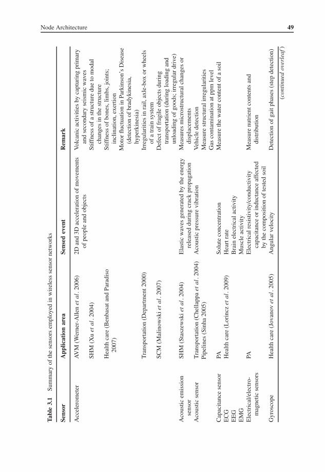
Node Architecture 49
Tabl
e3.
1Su
mm
ary
ofth
ese
nsor
sem
ploy
edin
wir
eles
sse
nsor
netw
orks
Sens
orA
pplic
atio
nar
eaSe
nsed
even
tR
emar
k
Acc
eler
omet
erA
VM
(Wer
ner-
Alle
net
al.2
006)
2Dan
d3D
acce
lera
tion
ofm
ovem
ents
ofpe
ople
and
obje
cts
Vol
cani
cac
tiviti
esby
capt
urin
gpr
imar
yan
dse
cond
ary
seis
mic
wav
esSH
M(X
uet
al.2
004)
Stif
fnes
sof
ast
ruct
ure
due
tom
odal
chan
ges
inth
est
ruct
ure
Hea
lthca
re(B
enba
sata
ndPa
radi
so20
07)
Stif
fnes
sof
bone
s,lim
bs,j
oint
s;in
clin
atio
n,ex
ertio
nM
otor
fluct
uatio
nin
Park
inso
n’s
Dis
ease
(det
ectio
nof
brad
ykin
esia
,hy
perk
ines
ia)
Tra
nspo
rtat
ion
(Dep
artm
ent2
000)
Irre
gula
ritie
sin
rail,
axle
-box
orw
heel
sof
atr
ain
syst
emSC
M(M
alin
owsk
iet
al.2
007)
Def
ecto
ffr
agile
obje
cts
duri
ngtr
ansp
orta
tion
(dur
ing
load
ing
and
unlo
adin
gof
good
s;ir
regu
lar
driv
e)A
cous
ticem
issi
onse
nsor
SHM
(Sta
szew
skie
tal
.200
4)E
last
icw
aves
gene
rate
dby
the
ener
gyre
leas
eddu
ring
crac
kpr
opag
atio
nM
easu
res
mic
rost
ruct
ural
chan
ges
ordi
spla
cem
ents
Aco
ustic
sens
orT
rans
port
atio
n(C
hella
ppa
etal
.200
4)Pi
pelin
es(S
inha
2005
)A
cous
ticpr
essu
revi
brat
ion
Veh
icle
dete
ctio
nM
easu
rest
ruct
ural
irre
gula
ritie
sG
asco
ntam
inat
ion
atpp
mle
vel
Cap
acita
nce
sens
orPA
Solu
teco
ncen
trat
ion
Mea
sure
the
wat
erco
nten
tof
aso
ilE
CG
Hea
lthca
re(L
orin
czet
al.2
009)
Hea
rtra
teE
EG
Bra
inel
ectr
ical
activ
ityE
MG
Mus
cle
acti
vity
Ele
ctri
cal/e
lect
ro-
mag
netic
sens
ors
PAE
lect
rica
lres
istiv
ity/c
ondu
ctiv
ityca
paci
tanc
eor
indu
ctan
ceaf
fect
edby
the
com
posi
tion
ofte
sted
soil
Mea
sure
nutr
ient
cont
ents
and
dist
ribu
tion
Gyr
osco
peH
ealth
care
(Jov
anov
etal
.200
5)A
ngul
arve
loci
tyD
etec
tion
ofga
itph
ases
(ste
pde
tect
ion)
(con
tinu
edov
erle
af)

50 Fundamentals of Wireless Sensor Networks
Tabl
e3.
1Su
mm
ary
ofth
ese
nsor
sem
ploy
edin
wir
eles
sse
nsor
netw
orks
(con
tinu
ed)
Sens
orA
pplic
atio
nar
eaSe
nsed
even
tR
emar
k
Hum
idity
sens
orPA
(Sze
wcz
yket
al.2
004)
HM
Rel
ativ
eas
wel
las
abso
lute
hum
idity
Infr
ason
icse
nsor
AV
M(W
erne
r-A
llen
etal
.200
6)C
oncu
ssiv
eac
oust
icw
aves
prod
uced
asa
resu
ltof
eart
hqu
ake
orvo
lcan
icer
uptio
nM
agne
ticse
nsor
Tra
nspo
rtat
ion
(Hao
uiet
al.2
008)
Pres
ence
,int
ensi
ty,d
irec
tion,
rota
tion,
and
vari
atio
nof
am
agne
ticfie
ldPr
esen
ce,s
peed
,and
dens
ityof
ave
hicl
eon
ast
reet
;con
gest
ion
Oxi
met
erH
ealth
care
(Mor
ris
and
Gui
lak
2009
)B
lood
oxyg
enat
ion
ofpa
tient
’she
mog
lobi
nC
ardi
ovas
cula
rex
ertio
n(s
tres
s)an
dtr
endi
ngof
exer
tion
rela
tive
toac
tivity
pHse
nsor
Pipe
line
(wat
er)
(Sto
iano
vet
al.2
007)
Con
cent
ratio
nof
hydr
ogen
ions
Indi
cate
sth
eac
idan
dal
kalin
eco
nten
tof
wat
er–
mea
sure
ofcl
eanl
ines
sPh
oto
acou
stic
spec
tros
copy
Pipe
line
(Sin
ha20
05)
Gas
sens
ing
Det
ects
gas
leak
ina
pipe
line
Piez
oele
ctri
ccy
linde
rPi
pelin
e(S
inha
2005
)G
asve
loci
tyA
leak
prod
uces
ahi
gh-f
requ
ency
nois
eth
atpr
oduc
esvi
brat
ion
Soil
moi
stur
ese
nsor
PA(L
opez
Riq
uelm
eet
al.2
009)
Soil
moi
stur
eFe
rtili
zer
and
wat
erm
anag
emen
tTe
mpe
ratu
rese
nsor
PA HM
(Lop
ezR
ique
lme
etal
.200
9)Te
mpe
ratu
re
Bar
omet
erse
nsor
PA HM
(Sze
wcz
yket
al.2
004)
Pres
sure
exer
ted
ona
fluid
Pass
ive
infr
ared
sens
orH
ealth
care
(Shn
ayde
ret
al.2
005)
HM
(Sze
wcz
yket
al.2
004)
Infr
ared
radi
atio
nfr
omob
ject
sM
otio
nde
tect
ion
Seis
mic
sens
orA
VM
(Wer
ner-
Alle
net
al.2
006)
Mea
sure
prim
ary
and
seco
ndar
yse
ism
icw
aves
(bod
yw
ave,
ambi
ent
vibr
atio
n)
Det
ectio
nof
eart
hqua
ke
Oxy
gen
sens
orH
ealth
care
(Mur
phy
and
Hei
nzel
man
2002
)A
mou
ntan
dpr
opor
tion
ofox
ygen
inth
ebl
ood
Blo
odflo
wse
nsor
Hea
lthca
re(M
urph
yan
dH
einz
elm
an20
02)
The
Dop
pler
shif
tof
are
flect
edul
tras
onic
wav
ein
the
bloo
d

Node Architecture 51
decision at this stage is to determine the number of allowable discrete values. This deci-sion in turn is influenced by two factors: (a) the frequency and magnitude of the signal;and (b) the available processing and storage resources.
2. The sampling frequency. In communication engineering and digital signal processing,this frequency is decided by the Nyquist rate.1 In wireless sensor networks, however, theNyquist rate does not suffice. Oversampling is required because of noise.The prevailing consequence of the first step is the quantization error while the second isaliasing.
An ADC is specified, among other things, in terms of its resolution, which is an expressionof the number of bits that can be used to encode the digital output. For example, an ADCwith a resolution of 24 bits can represent 16,777,216 distinct discrete values. The resolutionof an ADC can also be expressed in volts – since the output of most MEMS sensors is analogvoltage. The voltage resolution of an ADC is equal to its overall voltage measurement rangedivided by the number of discrete intervals. In other words:
Q = Epp
2M(3.1)
where Q is the resolution in volts per step (volts per output code); Epp is the peak-to-peakanalog voltage; and M is the ADC’s resolution in bits.
Here Q suggests that the interval between the discrete steps (values) is uniform. But inreality this is not so. In most ADCs, the least significant bit changes as a function of 0.5times Q and the most significant bit changes as a function 1.5 times Q. Those bits in themiddle have a resolution of Q voltage.
In selecting an ADC, knowledge of the process or activity being monitored is important.Consider an industrial process whose thermal property ranges from −20 to +80◦ C. Thechoice of the physical sensor as well as the ADC depends on the type of thermal change thatis of interest. If, for example, a change of 0.5 ◦C is required, an ADC with a resolution of8 bits is sufficient. If, on the other hand, a change of 0.0625 ◦C is required, then the ADCshould have a resolution of 11 bits.
3.2 The Processor Subsystem
The processor subsystem brings together all the other subsystems and some additionalperipherals. Its main purpose is to process (execute) instructions pertaining to sensing,communication, and self-organization. It consists of a processor chip, a nonvolatile memory(usually an internal flash memory) for storing program instructions, an active memory fortemporarily storing the sensed data, and an internal clock, among other things.
Whereas a wide range of off-the-shelf processors are available for building a wirelesssensor node, one has to make a careful choice, as it affects the cost, flexibility, performance,and energy consumption of the node. If the sensing task is well defined from the outset anddoes not change over time, a designer may choose either a field programmable gate arrayor a digital signal processor. These processors are very efficient in terms of their energyconsumption; and for most simple sensing tasks, they are quite adequate. However, as these
1 For a band-limited signal, the Nyquist rate sets a lower bound on the sampling frequency. Hence, the minimumsampling rate should be twice the bandwidth of the signal.

52 Fundamentals of Wireless Sensor Networks
are not general-purpose processors, the design and implementation process can be complexand costly.
In many practical cases, however, the sensing goal changes or a modification may berequired. Moreover, the software that runs on the wireless sensor node may require occa-sional updates or remote debugging. Such tasks require a considerable amount of com-putation and processing space at runtime. In which case, special-purpose, energy-efficientprocessors are not suitable.
Most existing sensor nodes at present use microcontrollers. There are some justificationsbesides those just mentioned. WSNs are emerging technologies; and the research communityis still active with research for developing energy-efficient communication protocols andsignal-processing algorithms. As this requires dynamic code installation and update, themicrocontroller is the best option.
3.2.1 Architectural Overview
A major concern in resource-constrained processors is the efficient execution of algorithms,since this requires the transferring of information from and to memory. This includes pro-gram instructions and the data to be processed or manipulated. For example, in WSNs, thedata stem from the physical sensors and the program instructions relate to communication,self-organization, data compression, and aggregation algorithms.
The processor subsystem can be designed by employing one of the three basic computerarchitectures: Von Neumann, Harvard, and Super-Harvard (SHARC). The Von Neumannarchitecture provides a single memory space that is used by program instructions and data.It provides a single bus to transfer data between the processor and the memory. This archi-tecture has a relatively slow processing speed because each data transfer requires a separateclock. Figure 3.2 illustrates a simplified view of the Von Neumann architecture.
The Harvard architecture modifies the Von Neumann architecture by providing separatememory spaces for storing program instructions and data. Each memory space is interfacedwith the processor with a separate data bus. In this way, program instructions and data canbe accessed at the same time. Additional to this feature, the architecture supports a specialsingle instruction, multiple data (SIMD) operation, a special arithmetic operation and a bitreverse addressing. It can easily support multitasking operating systems, but it has no virtualmemory or memory protection. Figure 3.3 displays the Harvard architecture.
Processor Memory
Address Bus
Data Bus
Figure 3.2 The Von Neumann architecture.

Node Architecture 53
DataMemory
Processor
Address Bus
Data Bus
ProgramMemory
Figure 3.3 A simplified view of the Harvard architecture.
The next generation of processor architecture is the Super-Harvard architecture, bestknown as SHARC. It is an extension of the Harvard system; it adds two essential compo-nents to its predecessor and provides alternatives for accessing I/O devices from within theprocessor subsystem. One of the components is an internal instruction cache that enhancesthe performance of the processor unit. It can be used to temporarily store frequently usedinstructions, thereby reducing the need for repeatedly fetching them from the program mem-ory. Moreover, the architecture enables an underutilized program memory to be used as atemporary relocation place for data.
In SHARC, external I/O devices can directly be connected with the memory unit throughan I/O controller. The configuration enables a direct data streaming from an external hard-ware into the data memory, without the need to involve the microcontroller. This is knownas Direct Memory Access (DMA).
DMA is desirable for two reasons: (1) the costly CPU cycles can be invested in a differenttask; and (2) it makes program memory bus and data memory bus accessible from outsidethe chip, providing an additional interface to off-chip memory and peripherals. Figure 3.4illustrates an overview of the SHARC architecture.
ProgramMemory
Processor
Instruction Cache
DataMemory
I/OController
Address Bus
Data Bus
Figure 3.4 An overview of the Super-Harvard architecture.
54 Fundamentals of Wireless Sensor Networks
3.2.2 Microcontroller
A microcontroller is a computer on a single integrated circuit, consisting of a compara-tively simple central processing unit and additional components such as high-speed buses,a memory unit, a watchdog timer, and an external clock. Microcontrollers are integratedin many products and embedded devices. Today such simple systems as elevators, venti-lators, office machines, household appliances, power tools, and toys ubiquitously employmicrocontrollers.
3.2.2.1 Structure of a Microcontroller
Typically, a microcontroller integrates the following components:
• a CPU core that ranges from small and simple 4-bit to complex 32- or 64-bit processors;• a volatile memory (RAM) for data storage;• a ROM, EPROM, EEPROM, or flash memory for storing relatively simple instruction
program code;• parallel I/O interfaces;• discrete input and output bits, allowing control or detection of the logic state of an indi-
vidual package pin;• a clock generator – which is often an oscillator with a quartz timing crystal;• one or more internal analog-to-digital converters; and• serial communications interfaces such as Serial Peripheral Interface and Controller Area
Network for interconnecting system peripherals such as event counters, a timer, and awatchdog.
3.2.2.2 Advantages and Disadvantages
A microcontroller can be chosen over other types of small-scale processors because of theprogramming flexibility it offers. Its compact construction, small size, low power consump-tion, and low cost make it suitable for building computationally less intensive, standaloneapplications. Most of the commercially available microcontrollers can be programmed withassembly language and the C programming language.
The use of higher-level programming languages increases the programming speed andeases debugging. There are development environments that offer an abstraction of all thefunctionalities of a microcontroller. This enables application developers to program micro-controllers without the need to have a low-level knowledge of the hardware.
However, microcontrollers are not as powerful and as efficient as some custom-madeprocessors such as digital signal processors (DSPs) and field programmable gate arrays(FPGAs). Moreover, for applications which demand simple sensing tasks but large-scaledeployments (such as in precision agriculture and active volcano monitoring), one may pre-fer to use architecturally simple but energy- and cost-efficient processors such as application-specific integrated circuits.
3.2.3 Digital Signal Processor
A comprehensive understanding of DSPs requires a knowledge of digital signal process-ing. Broadly speaking, digital signal processing deals with processing discrete signals with

Node Architecture 55
digital filters. These filters minimize the effect of noise on a signal or selectively enhance ormodify the spectral characteristics of a signal.
While analog signal processing requires complex hardware components, digital signalprocessing, on the contrary, requires mainly simple adders, multipliers, and delay compo-nents. A DSP is a specialized microprocessor designed to carry out complex mathematicaloperations at an extremely high efficiency, processing hundreds of millions of samplesevery second and providing real-time performance. Most commercially available DSPs aredesigned with the Harvard architecture.
3.2.3.1 Advantages and Disadvantages
Powerful and complex digital filters can be realized with commonplace DSPs. These filtersperform remarkably well in signal detection and estimation, both of which require significantnumerical computations. This is particularly interesting for multimedia WSN applicationsin which in-network audio and video signal processing may be required to compress oraggregate large size data. DSPs are also useful for applications that require the deploymentof nodes in harsh physical settings where signal transmission may suffer corruption due tonoise and interference.
Having said this, a WSN carries out other tasks (tasks pertaining to network management,self-organization, multi-hop communication, topology control, etc.) in addition to numeri-cal computations. These tasks require protocols which are not necessarily characterized asnumerical operations. Furthermore, the protocols may require periodical upgrade or modi-fications, which means flexibility in network reprogramming is vital.
3.2.4 Application-Specific Integrated Circuit
An application-specific integrated circuit (ASIC) is an integrated circuit (IC) that can becustomized for a specific application. There are two types of design approaches: fully cus-tomized and half-customized. To understand the difference between these two, it is usefulto understand the basic building blocks of an ASIC.
The ASIC architecture consists of cells and metal interconnects. A cell is an abstractionof a logical functionality that is physically implemented by active components (transistors).When several of these cells are interconnected by the metal interconnects, they make upan application-specific integrated circuit. The manufacturing of cells has reached such amaturity that there is a standard library of cells consisting of a collection of low-level logicfunctions, including basic gates (AND, OR, and INVERT), multiplexers, adders, and flip-flops. As the standard cells have identical size, they can be arranged in rows to ease theprocess of automated digital layout. Using predefined cells from a cell library makes theASIC design process much easier.
In a fully customized IC, some (possibly all) logic cells, circuits, or layouts are custommade. The aim is to optimize cell performance (for example, execution speed) and to includefeatures that are not defined or supported by the standard cell library. Fully customizedASICs are expensive and their design time is lengthy. On the other hand, a half-customizedASIC is built with logic cells that are available in the standard library.
In both cases, the final logic structure is configured by the end user. This reduces timeto market and financial risks by eliminating the need to cycle through an integrated circuit

56 Fundamentals of Wireless Sensor Networks
production. An ASIC is a cost-efficient solution, since the interconnections as well as thelogic structure can be specified according to the user’s needs. This also offers great flexibilityand reusability.
3.2.4.1 Advantages and Disadvantages of ASICs
Unlike a microcontroller, an ASIC can easily be designed and optimized to meet a specificcustomer demand. Even with a half-customized design, it is possible to design multiplemicroprocessor cores and embedded software in a single cell. Moreover, even thougha fully customized ASIC is costly, with a hybrid approach (full custom and standardcell design), developers can achieve control over size and execution speed. Thus, it ispossible to design with optimum performance and cost. Typical disadvantages includedifficulties in designing, the lack of reconfigurability, and the usually high developmentcosts.
3.2.4.2 Application of ASIC
Perhaps the most suitable role of ASICs in WSNs is not to replace microcontrollers orDSPs but to complement them. As briefly mentioned in the introduction section of thischapter, some of the subsystems may integrate customized processors to handle rudimentaryand low-level tasks and to decouple these tasks from the main processing subsystem. Forexample, some communication subsystems are shipped with an embedded processor coreto enhance the quality of received signals, cancel noise, and perform cyclic redundancychecks. These types of special-purpose processors can be efficiently realized by making useof ASICs.
3.2.5 Field Programmable Gate Array
The distinction between ASICs and FPGAs is not always clear. In fact, it is not unusualfor companies that manufacture programmable ASICs to call their products FPGAs. Whilethe basic anatomy of both architectures is essentially the same, FPGAs are more complexin design and more flexible to program. As the emphasis is on the (re)programming andreconfigurability aspect, typical features of a FPGA are summarized as follows:
• in a FPGA, none of the mask layers is customized;• a FPGA includes some programmable logic components, or logic blocks – these are: a
4-input lookup table (LUT), a flip-flop, and an output block;• there is a well-defined and formal method for programming the basic logic cells and the
interconnect;• there is a matrix of programmable interconnects surrounding the basic logic cells produc-
ing a configuration instance; and• there are programmable I/O cells that surround the core.
FPGAs are programmed electrically, by modifying a packaged part. This process maytake from a few milliseconds to a few minutes, depending on the programming technology

Node Architecture 57
and the size of the part. The programming is done with the support of circuit diagrams andhardware description languages, such as VHDL and Verilog.
3.2.5.1 Advantages and Disadvantages
FPGAs have a higher bandwidth compared to DSPs; they are more flexible in their applica-tion and can support parallel processing. While DSPs and microcontrollers can incorporatean internal ADC, a FPGA does not. Similar to a DSP, a FPGA has the capability to work withfloating point representation. Additionally, a FPGA exposes its processing speed to appli-cation developers, thereby giving them a greater flexibility of control. On the other hand,FPGAs are complex; and the design and realization process is costly.
3.2.6 Comparison
Working with a microcontroller is preferred if the design goal is to achieve flexibility. Work-ing with all the others is preferred if power consumption and computational efficiency isdesired. Whereas microcontrollers have limited memory, steady progress is being made toincrease memory size. Recently, more and more microcontrollers are becoming available onthe market with attractive features; for example, the TI MSP430F2618 and MSP430F5437offer an active memory (RAM) of 8 kilobytes (KB) and 16 KB, as well as 116 KB and256 KB flash memory respectively. Both consume less power and perform better than ear-lier models. The Atmel ATMega1281 and its next version ATMega2561 also have goodarchitecture and better memory and performance. Both of them have 8 KB active mem-ory and 128 KB and 256 KB flash memory, respectively. The Jennic architecture – JN5121and JN5139 – integrates a microprocessor and a radio subsystem into a single package toenhance processing speed. It has 96 KB and 192 KB RAM, respectively; and 128 KB flashmemory.
In comparison, DSPs are expensive, large in size, and less flexible. For example the PIC16F873 and Sx28AC microcontrollers have 5 million instructions per second (MIPs) and75 MIPS processing power; 24 and 20 general purpose I/O; 4 KB and 2 KB RAM, respec-tively; and 28-pin each. The devices cost around $5.81 and $4.05, respectively. Compared tothat, the DSP56364 has 100 MIPS processing power, 16 general-purpose I/O, 1 KB RAM,100 or 112-pin and costs $11.00. Moreover, DSPs are best for signal processing, with specificalgorithms.
FPGAs are faster than both microcontrollers and digital signal processors and supportparallel computing. In wireless sensor networks, since sensing, processing, and communi-cation should take place at the same time, FPGSs can be useful. However, their productioncost and the difficulty with programming make them less desirable.
ASICs have higher bandwidths; they are the smallest in size, perform much better, andconsume less power than any of the other processing types. Their main disadvantage is thehigh cost of production owing to the complex design process, usually with lower produc-tion quantity and a reduced reusability. Performance can be improved with the applicationof multicore systems where several applications could run in parallel. This enables the inte-gration of ASICs into the other subsystems, so that when the main processor subsystem isidle and therefore should be turned off, elementary and rudimentary tasks can be carried outby the more efficient ASICs.

58 Fundamentals of Wireless Sensor Networks
3.3 Communication Interfaces
As the selection of the right type of processor is vital to the performance as well as the energyconsumption of a wireless sensor node, the way the subcomponents are interconnected withthe processor subsystem is also vital.
Fast and energy-efficient data transfer between the subsystems of a wireless sensor nodeis critical to the overall efficiency of the network it sets up. However, the practical size ofthe node puts a restriction on system buses. Whereas communication via a parallel bus isfaster than a serial bus, a parallel bus needs more space. Moreover, it requires a dedicatedline for every bit that should be transmitted simultaneously while the serial bus requires asingle data line only. Owing to the size of the node, parallel buses are never supported innode design.
The choice, therefore, is often between serial interfaces such as the serial peripheral inter-face (SPI), the general purpose input/output (GPIO), the secure data input/output (SDIO),the inter-integrated circuit (I2C), and the Universal Serial Bus (USB). Among these, themost commonly used buses are the SPI and the I2C.
3.3.1 Serial Peripheral Interface
The Serial Peripheral Interface (SPI – pronounced as “spy”) is a high-speed, full-duplexsynchronous serial bus. It was developed at Motorola in the mid-1980s. It does not have anofficial standard as such, but manufacturers building devices that use the SPI should conformto the implementation specification of other manufacturers in order to support correct com-munication (for example, devices should agree on whether to transmit the most significantbit (MSB) or the least significant bit (LSB) first).
The SPI bus defines four pins: (Master-Out/Slave-In) MOSI, (Master-In/Slave-Out)MISO, (Serial Clock) SCLK, and (Chip Select) CS. Some manufacturers refer to MOSI asSIMO and to MISO as SOMI, but the semantics is the same. Likewise, CS is sometimesreferred to as (Slave Select) SS. As the name suggests, MOSI is used to transmit datafrom the master to the slave when a device is configured as a master. In case it isconfigured as a slave, this port is used to receive data from the corresponding master.The semantics are reversed for the MISO port. SCLK is used by the master to send theclock signal that is needed to synchronize transmission; and by the slave to read thissignal. Every communication is initiated by the master. A master device signals a slavewith which it wants to communicate via the CS port. Since SPI is a single master bus, themicrocontroller is by default the master in a wireless sensor node. Thus, components cannotcommunicate directly with each other but only via the microcontroller – for example, withthis configuration, an ADC cannot send a sampled data directly to a RAM. Figure 3.5illustrates two types of configurations. In (a), a single master communicates with a singleslave device, while in (b), a master is connected with multiple slave devices.
Both master and slave devices hold shift registers. In most cases these are 8-bit registers,but heterogeneous sizes are also allowed. Both registers are connected in a ring-forming16-bit shift register. This is the common mode of connection. Assuming that the MSB istransferred first, during a transmission cycle, the MSB that is sent by the master is insertedto the slave’s LSB register while, in the same cycle, the slave’s MSB is shifted to the master’s

Node Architecture 59
Master
Master
Slave
Slave 1
Slave 2
Slave 3
SCLK
SCLK
MOSI
MOSI
MISO
(a)
MISO
SS
SCLKMOSIMISOSS
SCLKMOSIMISOSS
SCLKMOSIMISOSS
SS1SS2SS3
(b)
Figure 3.5 Connecting devices with the SPI bus. (a) A single master connecting with a single slave.(b) A single master connecting with multiple slaves.
LSB. After all bytes have been sent, the slave’s register contains the master’s word, whilethe master holds the slave’s word.
Since master and slave form a commonly used shift register, every device in every trans-mission must read and send data. For devices that do not provide feedback (for example,LC displays do not offer status or bug messages) or do not require input data (some devicesmay not accept any commands at all), this means adding pseudo bytes into the shift register.
SPI supports a synchronous communication protocol. Consequently, the master and theslave must agree on the timing. To do so, the master sets the clock according to the slave’smaximum clock speed – the baud generator of the master reads the slave’s clock and cal-culates the master’s clock by dividing the read speed with an internally defined value.Furthermore, master and slave should agree on two additional parameters, namely, clockpolarity (CPOL) and clock phase (CPHA). CPOL defines whether a clock is used in high-or low-active mode. CPHA determines the times when the data in the registers are allowed tochange and when the written data can be read. There are four different combinations (shownin Table 3.2) which are all incompatible with each other.
3.3.2 Inter-Integrated Circuit
The inter-integrated circuit (I2C) is a multi-master half-duplex synchronous serial bus (seeFigure 3.6). It was developed by Philips Semiconductors, which is also the owner of theofficial standard. I2C uses only two bidirectional lines (unlike SPI, which uses four). The

60 Fundamentals of Wireless Sensor Networks
Table 3.2 Common SPI modes
SPI mode CPOL CPHA Description
0 0 0 SCLK is low-active.Sampling is allowed on odd clock edges.Data changes on even clock edges.
1 0 1 SCLK is low-active.Sampling is allowed on even clock edges.Data changes on odd clock edges.
2 1 0 SCLK is high-active.Sampling is allowed on odd clock edges.Data changes on even clock edges.
3 1 1 SCLK is high-active.Sampling is allowed on even clock edges.Data changes on odd clock edges.
Master
Slave Slave Slave
SCL
SDA
Figure 3.6 Connecting devices with the I2C serial bus.
aim of I2C is to minimize costs for connecting devices within a system by accommodatinglower transmission speeds. I2C defines two speed modes: a Fast-mode, with a bit rate of upto 400 kbps and a High-speed-mode (referred to as Hs-mode) that supports a transmissionrate of up to 3.4 Mbps. The 100 kbps rate (Standard-mode) was defined in earlier versions.Nevertheless, Fast-mode and Hs-mode components are downwards compatible to ensurecommunication with older components.
As the standard does not specify a CS or SS port, every device type that uses I2C musthave a unique address that will be used to communicate with a device. In earlier versions, a7-bit address was used, allowing 112 devices to be uniquely addressed (4 bits are reserved).This address space turned out to be insufficient due to an increasing number of devices.Currently I2C uses 10-bit addressing.
In the old protocol, a master device flags the start condition(s) and transmits the slave’s7-bit address. Then the master expresses read or write interest. At this time, the slave sendsan acknowledgment (ACK). Afterwards, the data transmitter sends a 1-byte (8-bits) data,which is then acknowledged by the receiver. If there is still data to be sent, the transmitterkeeps on sending and the receiver keeps on acknowledging in return. Finally, the masterraises the stop flag (stop condition) to signify the end of a communication.
In the new protocol, after the start condition (S), a leading 11110 introduces the 10-bitaddressing scheme. The last two address bits of the first byte concatenated with the eightbits of the second byte form the whole 10-bit address. Devices that only use 7-bit addressingsimply ignore messages with the leading 11110.

Node Architecture 61
Start(by the master)
Read or write(by the master)
Stop(by the master)
Acknowledge
LSB
(a)
(b)
Bit 9MSB
Bit 9MSB
Bit 0LSB
Bit 0LSB
LSB
Slaveaddress
Data(by the transmitter)
Data(by the transmitter)
LSBMSB
S
S 1 1 1 1 0 x x x x x x x x x x
x x x x x x x x x x
P
P
MSB MSB
W/R
ACK
W/R
ACK
ACK
ACK
ACK
ACK
Figure 3.7 Communication protocols in the I2C serial bus.
Figure 3.7 shows the old and the new I2C protocol. In (a) the old protocol is displayed.In (b) the new protocol is displayed with the first two bytes of a transfer and the 10-bitaddress.
As already mentioned, I2C provides two lines; these are Serial Clock (SCL) and SerialData Analyzer (SDA). Hs-mode devices have additional ports called SDAH and SCLH.Since each master generates its own clock signal, communicating devices must synchronizetheir clock speeds. In case they do not, a slower slave device could wrongly detect its addresson the SDA line while a faster master device is sending data to a third device. Besides clocksynchronization, I2C requires arbitration between master devices wanting to send or receivedata at the same time. I2C does not explicitly define any fair arbitration algorithm. Ratherthe master that holds the SDA line low for the longest time wins the medium. Additionally,I2C enables a device to read data at a byte level for fast communication. This, however,may raise the need for more time to store the received bytes, in which case the device canhold the SCL low until it completes reading or sending the next byte. This type of clocksynchronization is called handshaking.
Table 3.3 gives a comparison between SPI and I2C.
3.3.3 Summary
Buses are essential highways to transfer data between the processor subsystem and the othersubsystems. Due to the concern for size, only serial buses can be used by a wireless sen-sor node. These buses demand high clock speeds to gain the same throughput that can be

62 Fundamentals of Wireless Sensor Networks
Table 3.3 Comparison of SPI and I2C
SPI I2C
• Four lines enable full-duplex transmission.
• No addressing is required due to CS. Thisreduces overhead and increases throughput.However, one needs additional hardwareconfigurations to connect more than one slave.
• Allowing only one master avoids conflicts.
• Hardware requirement support increases withan increasing number of connected devicesand therefore raises costs.
• The master’s clock is configured according tothe slave’s speed. This frees the slaves fromrequiring clocking a device. However, speedadaptation slows down the master.
• Speed depends on the maximum speed of theslowest device.
• Heterogeneous register size allows flexibilityin the devices that are supported.
• Combined registers imply every transmissionshould be read.
• The absence of an official standard leads toapplication specific implementations.
• Two lines reduce space and simplify circuitlayout. Lowers costs.
• Addressing enables multimaster mode, whichin turn enables more than one device toinitiate communication.
• Multimaster mode is prone to conflicts whentwo or more master devices communicatesimultaneously. Arbitration is required.
• Hardware requirement is independent of thenumber of devices using the bus.
• Slower devices may stretch the clock therebyincreasing latency and keeping other deviceswaiting for accessing the bus.
• Speed is limited to 3.4 MHz and all devicesneed to support the highest speed that is usedin the system, otherwise a slower device maywrongly detect its device address.
• Homogeneous register size reduces overhead,since no additional control bits are required tobe transmitted.
• Devices that do not read or provide data arenot forced to provide potentially useless bytes.
• Official standard eases integration of devicessince developers can rely on a certainimplementation.
achieved with parallel buses. However, they can also be bottlenecks; this is particularly thecase with the Von Neumann architecture, since the same bus is used for data as well asinstructions. They also do not scale well with processor speed. For example I2C in its lat-est version is limited to 3.4 MHz while the clock speed of one of the most commonly usedmicrocontroller family, the TI MSP430x1xx series, has a clock frequency of 8 MHz.
Delays due to contention for bus access become critical if some of the devices act unfairlyand keep the bus occupied. For example, I2C allows slave devices to stretch clock signalsif it is deemed appropriate to “packet” communication and give priority to components thatneed to exchange time-critical data.
3.4 Prototypes
In this section, some example prototype node architectures are presented. The architecturesare not chosen because of their commercial success or energy efficiency, but because theydemonstrate the different node realization possibilities discussed in the preceding section.

Node Architecture 63
3.4.1 The IMote Node Architecture
The IMote sensor node architecture (Figure 3.8) is a multipurpose architecture that con-sists of a power management subsystem, a processor subsystem, a sensing subsystem, acommunication subsystem, and an interfacing subsystem.
The sensing subsystem (Figure 3.9) provides an extensible platform to connect multiplesensor boards. One realization of the sensor board contains a 12-bit, 4-channel ADC; a high-resolution temperature/humidity sensor; a low-resolution digital temperature sensor; and alight sensor. These devices are interfaced to the processing subsystem through the SPI andI2C buses. As can be seen in the figure, the I2C bus is chosen to connect low data rate sourceswhereas the SPI bus is used to interface high data rate sources.
The processing subsystem provides a main processor (microprocessor) and a digital signalprocessor (DSP). The main processor has the ability to operate at a low-voltage (0.85 V)and a low-frequency (13 MHz) mode, thus enabling low power operation. Likewise, thefrequency can be scaled to 104 MHz at the lowest voltage level and can be increased up to416 MHz with Dynamic Voltage Scaling (DVS). Moreover, it has many low power modes,including sleep and deep sleep modes.The coprocessor is intended to accelerate multimediaoperations, which are computation intensive.
802.15.4radio
XScaleCPU core
XScaleDSP
Antenna
SMA
256KB SRAM
32MBFLASH
32MBSDRAM
Powermanagement
I/O
GPIOs
2x SPI
3x UART
I2C
RTC
SDIO
USB host
USB client
AC’97
Camera
I2S
Supply Batterycharger
Figure 3.8 The architecture of an IMote sensor node.

64 Fundamentals of Wireless Sensor Networks
HumidityTemperature
3DAccelerometer
Power regulator
ADC
External connector
Temperature Light
GPIO
SPI
I2C
Figure 3.9 The sensing subsystem of the IMote architecture.
Similar to the sensor subsystem, the communication subsystem provides an extensibleinterface to accommodate different types of radios. One realization is based on the Chip-con (CC2420) transceiver, which implements the IEEE 802.15.4 radio specification. Thetransceiver provides a transmission rate of 250 kbps over 16 channels in the 2.4-GHz band.
3.4.2 The XYZ Node Architecture
The XYZ architecture consists of four subsystems. Figure 3.10 shows the schematic dia-gram of the node architecture. The processor subsystem is based on the ARM7TDMI coremicrocontroller, which is capable of operating at a maximum frequency of 58 MHz. Themicrocontroller can operate at two different modes, depending on the application require-ment: at 32 bits and 16 bits. The processing subsystem provides an on-chip memory of 4 KBboot ROM and a 32 KB RAM, which can be extended by up to 512 KB of flash memory.
The peripheral components that interface the processing subsystem with the remainingsubsystem include an embedded DMA controller, four 10-bit ADC inputs, serial ports(RS232, SPI, I2C, SIO), and 42 multiplexed general-purpose I/O pins. Most of themultiplexed GPIO pins are available on two 30-pin headers together with the DC voltageprovided by the power subsystem or directly by an on-board voltage regulator.
The communication subsystem is based on the Chipcon CC2420 radio, which is con-nected to the processing subsystem through a SPI interface. The CC2420 is a 2.4 GHz IEEE802.15.4 compliant single-chip RF transceiver. The processor subsystem controls the com-munication subsystem by either turning it off or putting it in sleep mode. The communicationthrough the SPI interface enables the radio to wake up a sleeping processor when an RFmessage has been successfully received.

Node Architecture 65
OKI ML67Q500x
Battery(3 x AA)
VoltageRegulator
Supervisor
ChipconCC2420
(802.15.4)
3.3V 2.5V
ON/OFF
PowerTrackingInterface
Core: 2.5V
I/O: 3.3V
3.3V
WAKE UP
INT
GPIO & Peripheral Connectors
SRAM256K x 16
Light Sensors Array
Thermometer
Accelerometer
H-bridge Geared Motor
Inertial StringTrackerCamera
I2C
SPI ON/OFF
PowerSubsystem
CommunicationSubsystem
SensorSubsystem
MobilitySubsystem
Figure 3.10 The XYZ node architecture (Lymberopoulos and Savvides 2005).
While in the architecture the mobility subsystem appears to be a separate subsystem, itshould be considered as a part of the sensor subsystem.
3.4.3 The Hogthrob Node Architecture
The Hogthrob node architecture (Bonnet et al. 2006) is designed for a specific application,namely, to monitor the activities of sows in a large-scale pig production. The basic assump-tion behind the main sensing task is that there is a direct correlation between the movementof a sow and the onset of estrus. Therefore, a network that is established by nodes worn bysows monitors movements to capture this vital state, so that appropriate care can be givenfor pregnant sows. For example, in Denmark a law is already in place that requires pregnantsows to move freely in a large pen. Apart from this, other vital conditions, such as illness(by detecting cough or limping), are also monitored by the sensor network.
The node architecture consists of the usual subsystems. Unlike many existing architec-tures, the Hogthrob node’s processing subsystems consists of two processors, a microcon-troller, and a field programmable gate array (FPGA). The microcontroller performs lesscomplex, less energy-intensive tasks, such as controlling the communication subsystem andother peripherals. It also initializes the FPGA and functions as an external timer and anADC converter to it. The FPGA executes the sow monitoring application and coordinatesthe functions of the sensor node.
Figure 3.11 displays a partial view of the node architecture and the various interfacingbuses. There are a number of interfaces supported by the processing subsystem, including theI2C interface for the sensing subsystem, the SPI for the communication subsystem, the JTAG

66 Fundamentals of Wireless Sensor Networks
Processorsubsystem
UART
UART ProgramFlash
AVRProcessor
Core
ADCSRAM
JTAG
CLK48MHz
Sensingsubsystem
I2C
ATMega 128L CLK8MHz PB LED 3V
1.2VMAX192R
2.5V MAX192R
CLK4MHz
CommunicationsubsystemBus
ExchangeSwitch
UART
UART
UART
FPGA Core
JTAG
SPI
SPI
SPI
Figure 3.11 A partial view of the Hogthrob node architecture (Bonnet et al . 2006).
interface for in-system programmability and debugging, and the serial (RS-232) interfacefor interaction with a PC.
Exercises
3.1 A vibration sensor outputs an analog signal with a peak-to-peak voltage of 5 V at afrequency of 100 Hz.
(a) What should be the minimum sampling frequency, so that no information is lostduring the digitization process?
(b) Suppose a resolution of 0.025 V is required to detect an interesting event. Whatshould be the resolution of the ADC in terms of bits to convert the analog signalto a digital signal?
3.2 What is the drawback of using a multichannel ADC?
3.3 What is aliasing?
3.4 Define each of the following terms as applied to discrete time signal processing sys-tems:
(a) Linearity

Node Architecture 67
(b) Time-invariance
(c) Causality
(d) Stability
3.5 While they are not the most energy-efficient solutions, microcontrollers are the pre-dominant processors in wireless sensor networks. Explain some of the reasons.
3.6 Explain the reason why using the Von Neumann architecture is not efficient for a wire-less sensor node.
3.7 Why are parallel buses not desirable in a wireless sensor node?
3.8 What is the side effect of using a serial bus that supports full-duplex communication?
3.9 Explain the following terms in the context of the serial bus, SPI:
(a) Serial Data Out
(b) Serial Data In
(c) Serial Clock
3.10 State how a master component can communicate with multiple slaves in:
(a) I2C
(b) SPI
3.11 Explain, with the help of diagrams, how the data transfer protocol of the I2C bus func-tions.
3.12 Explain the basic similarities and differences between a FPGA and an ASIC.
3.13 Explain some of the distinct features of the Super-Harvard architecture.
3.14 A large number of commercially available wireless sensor nodes integrate three typesof memory architectures: EEPROM (flash memory), RAM, and ROM. Explain thepurpose of each of them.
3.15 The communication subsystem of a wireless sensor node is usually interfaced with theprocessor subsystem through a SPI bus instead of an I2C bus. Why is this?
3.16 While memory management is very useful, it cannot be supported in wireless sensornetworks. Why?
3.17 What is a virtual memory?
3.18 In most communication systems, the last stage in the reception process requires digital-to-analog converters (DAC). But in this book, the DAC is not discussed. What do youthink is the reason?
3.19 Explain two different ways of interfacing an analog temperature sensor with a proces-sor subsystem.
3.20 How can two hardware components with different speeds communicate with eachother through a serial bus?

68 Fundamentals of Wireless Sensor Networks
ReferencesBenbasat, A.Y., and Paradiso, J.A. (2007) A framework for the automated generation of power-efficient classi-
fiers for embedded sensor nodes. SenSys ’07: Proceedings of the 5th International Conference on EmbeddedNetworked Sensor Systems (pp. 219–232). ACM, New York, NY, USA.
Bonnet, P., Leopold, M., and Madsen, K. (2006) Hogthrob: Towards a sensor network infrastructure for sow moni-toring (wireless sensor network special day). DATE ’06: Proceedings of the Conference on Design, Automationand Test in Europe (p. 1109). European Design and Automation Association, 3001 Leuven, Belgium.
Chellappa, R., Qian, G., and Zheng, Q. (2004) Vehicle detection and tracking using acoustic and video sensors.Proc. of IEEE Conf. on Acoustics, Speech, and Signal Processing.
Department UT (2000) Developed wheel and axle assembly monitoring system to improve passenger train safety.Haoui, A., Kavaler, R., and Varaiya, P. (2008) Wireless magnetic sensors for traffic surveillance. Transportation
Research Part C: Emerging Technologies . 16 (3), 294–306.Jovanov, E., Milenkovic, A., Otto, C., and de Groen, P.C. (2005) A wireless body area network of intelligent motion
sensors for computer assisted physical rehabilitation. Journal of Neuro-Engineering and Rehabilitation . 2: 6.Lopez Riquelme, J.A., Soto, F., Suardıaz, J., Sanchez, P., Iborra, A., and Vera, J.A. (2009) Wireless sensor networks
for precision horticulture in southern Spain. Comput. Electron. Agric. 68 (1), 25–35.Lorincz, K., Chen, Br., Challen, G.W., Chowdhury, A.R., Patel, S., Bonato, P., and Welsh, M. (2009) Mercury:
A wearable sensor network platform for high-fidelity motion analysis. SenSys ’09: Proceedings of the 7th ACMConference on Embedded Networked Sensor Systems (pp. 183–196). ACM, New York, NY, USA.
Lymberopoulos, D., and Savvides, A. (2005) XYZ: A motion-enabled, power aware sensor node platform fordistributed sensor network applications. IPSN ’05: Proceedings of the 4th International Symposium on Infor-mation Processing in Sensor Networks (p. 63). IEEE Press, Piscataway, NJ, USA.
Malinowski, M., Moskwa, M., Feldmeier, M., Laibowitz, M., and Paradiso, J.A. (2007) Cargonet: A low-costmicropower sensor node exploiting quasi-passive wakeup for adaptive asynchronous monitoring of exceptionalevents. SenSys ’07: Proceedings of the 5th International Conference on Embedded Networked Sensor Systems(pp. 145–159). ACM, New York, NY, USA.
Morris, M., and Guilak, F. (2009) Mobile heart health: Project highlight. IEEE Pervasive Computing 8 (2), 57–61.Murphy, A.L., and Heinzelman, W.B. (2002) MiLAN: Middleware linking applications and networks . Technical
Report, Rochester, NY, USA.Shnayder, V., Chen, Br., Lorincz, K., Jones, T.R.F.F., and Welsh, M. (2005) Sensor networks for medical care.
SenSys ’05: Proceedings of the 3rd International Conference on Embedded Networked Sensor Systems(p. 314). ACM, New York, NY, USA.
Sinha, D.N. (2005) Acoustic sensor for pipeline monitoring . Technical Report, Los Alamos National Laboratory.Stoianov, I., Nachman, L., Madden, S., and Tokmouline, T. (2007) Pipenet: A wireless sensor network for pipeline
monitoring. IPSN ’07: Proceedings of the 6th International Conference on Information Processing in SensorNetworks (pp. 264–273). ACM, New York, NY, USA.
Szewczyk, R., Mainwaring, A., Polastre, J., Anderson, J., and Culler, D. (2004) An analysis of a large scale habitatmonitoring application. SenSys ’04: Proceedings of the 2nd International Conference on Embedded NetworkedSensor Systems (pp. 214–226). ACM, New York, NY, USA.
Werner-Allen, G., Lorincz, K., Welsh, M., Marcillo, O., Johnson, J., Ruiz, M., and Lees, J. (2006) Deploying awireless sensor network on an active volcano. IEEE Internet Computing 10 (2), 18–25.
Staszewski, W.J., Boller, G., and Tomlinson, G. (eds) (2004) Health Monitoring of Aerospace Structures: SmartSensor Technologies and Signal Processing . John Wiley & Sons Ltd.
Xu, N., Rangwala, S., Chintalapudi, K.K., Ganesan, D., Broad, A., Govindan, R., and Estrin, D. (2004) A wirelesssensor network for structural monitoring. SenSys ’04: Proceedings of the 2nd International Conference onEmbedded Networked Sensor Systems (pp. 13–24). ACM, New York, NY, USA.

4Operating SystemsAn operating system (OS) in a WSN is a thin software layer that logically resides betweenthe node’s hardware and the application and provides basic programming abstractions toapplication developers. Its main task is to enable applications to interact with hardwareresources, to schedule and prioritize tasks, and to arbitrate between contending applicationsand services that try to seize resources. Additional features include:
• memory management;• power management;• file management;• networking;• a set of programming environments and tools – commands, command interpreters, com-
mand editors, compiler, debuggers, etc. – to enable users to develop, debug, and executetheir own programs; and
• legal entry points into the operating system for accessing sensitive resources such aswriting to input components.
Traditionally, operating systems are classified as single-task/multitasking and single-user/multi-user operating systems. A single-task operating system processes one task ata time while a multitasking operating system can execute multiple tasks simultaneously.Multitasking operating systems require a large amount of memory to manage the statesof multiple tasks but they enable tasks with different complexity to execute in parallel.For example, in a wireless sensor node, the processor subsystem may interact with thecommunication subsystem while aggregating data that arrive from the sensing subsystem.A multitasking OS is the best candidate for this type of environment. However, due tothe limited resources, the overhead of concurrent processing may not be affordable. Ina single-task OS one task is executed at a time, therefore, as a rule tasks should have ashort duration. In a single-user OS, one user (the owner of the resources) is active at atime, whereas a multi-user operating system allows multiple users to share the resourcesof a single system at the same time.
The choice of a particular operating system depends on several factors. In the followingsections, typical functional and nonfunctional aspects will be discussed.
Fundamentals of Wireless Sensor Networks: Theory and Practice Waltenegus Dargie and Christian Poellabauer 2010 John Wiley & Sons, Ltd

70 Fundamentals of Wireless Sensor Networks
4.1 Functional Aspects
4.1.1 Data Types
In wireless sensor networks (WSNs), communication between the different subsystemsis vital. These subsystems communicate with each other for various reasons such as toexchange data, delegate functionalities, and signaling. Interactions take place throughwell-formulated protocols and data types that are supported by the OS. Complex datastructures have strong expression power but consume resources, while simple data typesare resource efficient but have limited expression capability. Almost all of the exist-ing operating systems or runtime environments in WSNs support the native data typesof the C programming language and some of the complex data types such as structand enum .
4.1.2 Scheduling
Task scheduling is one of the basic functions of an OS. How efficiently tasks can beorganized, prioritized, and executed determines the efficiency of the OS.
Broadly speaking, there are two scheduling mechanisms: queuing-based and round-robin scheduling. In a queuing-based scheduling, tasks originating from the varioussubsystems are temporarily stored in a queue and executed serially according to a prede-fined rule. Some operating systems enable tasks to specify priority levels so that they canbe given precedence.
Queuing-based scheduling can be further classified into first-in-first-out (FIFO) andsorted queue. In a FIFO scheme, tasks are processed according to their arrival time: a taskthat arrives first will be executed first as soon as the processor is free. A nonpreemptiveOS will execute the task to the end before another task is admitted for execution. In apreemptive OS, however, a task of higher priority may interrupt a task of low priority. Ina sorted queue scheme, tasks in a queue are sorted according to some criteria. One wayis to sort tasks according to their estimated execution duration. This approach preventslong-duration tasks from blocking short-duration tasks. The approach is also known asthe shortest job first (SJF) rule.
The FIFO scheme is the simplest and the most economical as it incurs minimum systemoverheads. However, the FIFO scheme may not treat tasks fairly, since tasks of longduration may block short-duration tasks for a long time. In the SJF scheme, sorting incurssystem overhead, since each task in the queue must be evaluated to estimate executionduration and to sort tasks accordingly.
Round-robin scheduling is a time-sharing scheduling technique in which several taskscan be processed concurrently. The scheduler defines a time frame by dividing time intoslots and tasks will be given slots in a multiplexed manner. This way, all the tasks advancetoward their completion.
Regardless of how tasks are executed, a scheduler can be either a nonpreemptive or pre-emptive scheduler. In strictly nonpreemptive scheduling, a task is executed to the end andwill not be interrupted by another task. On the contrary, in strictly preemptive scheduling,the scheduler decides how time is shared between tasks and allows a task of higher prior-ity to interrupt a task of lower priority. There is also the so-called “politely-preemptive”
Operating Systems 71
scheduling in which, even if tasks are interruptible, the scheduler will not interrupt aprocess if it is in a critical section.
4.1.3 Stacks
A stack is a data structure that is used to temporarily store data objects in memory bypiling one upon another. The objects are accessed on a last-in first-out (LIFO) basis.The processor core uses stacks to store system state information when it begins exe-cuting subroutines. This way it “remembers” where to return after the subroutine iscompleted. Subroutines can also call other subroutines by storing the state of the currentsubroutine on top of the previous state information in the stack. When the subroutine iscompleted, the processor pulls the first address it finds on the top of the stack and jumps tothat location.
In a multithreaded OS, each thread requires its own stack to manage state information.This is one of the reasons why multithreaded operating systems are expensive in WSNs.
4.1.4 System Calls
The OS provides a number of basic functions which enable the separation of concern,namely, the need to decouple the concern of accessing hardware resources and addi-tional low-level services from the implementation details of the access mechanisms.Users invoke these operations whenever they wish to access a hardware resource such as asensor, watchdog timer, or the radio without the need to concern themselves how the hard-ware is accessed. In a UNIX environment, these basic functions are commonly known assystem calls.
4.1.5 Handling Interrupts
An interrupt is an asynchronous signal generated by a hardware device (a sensor, awatchdog timer, a radio) and causes the processor to interrupt executing the presentinstruction and to call for an appropriate interrupt handler. The processor stores the stateof the interrupted process in a stack and gives control to the interrupt handler. For example,an interrupt signal may be raised by the communication subsystem when it receives apacket that should be processed immediately. The processor subsystem must then suspendthe execution of the present instruction and calls for the appropriate module in the OS thatshould handle radio packets. Additional to the hardware devices, the OS can define severalsystem events that can flag interrupt signals. In some cases, the OS itself can generateperiodic interrupts to allow the processor to monitor the state of hardware resources andinform corresponding event handlers in case there is an interest in a specific hardware state.
In the same way that tasks can have different priority levels, interrupt signals canalso have different priority levels. A high-priority interrupt can interrupt a low-priorityinterrupt. In such systems, programs can choose whether or not they wish to be interruptedby setting an interrupt mask. The mask enables them to “evade” low-level interrupts thatthey have nothing to do with. Masking interrupts can be dangerous and can corrupt data.Some operating systems have nonmaskable interrupts for the most crucial operations.

72 Fundamentals of Wireless Sensor Networks
4.1.6 Multithreading
A thread is the path taken by a processor or a program during its execution. In a single-task,nonpreemptive operating systems, tasks are monolithic and there is only a single threadof execution. In a multithreaded environment, a task can be divided into several logicalpieces which can be scheduled independently from each other and executed concurrently.Likewise, multiple tasks originating from different sources can be executed concurrentlyin multiple threads. Threads of the same task share a common data and address spaceand can communicate with each other if necessary. There are two main advantages of amultithreaded OS:
1. tasks do not block other tasks; this is particularly important to deal with tasks pertainingto I/O systems;
2. short-duration tasks can be executed along with long-duration tasks.
While threads are resource conservative by nature, they cannot be created endlessly.The creation of threads slows down the processor and there may not be sufficient resourcesto divide among a large number of threads. Therefore, some operating systems supportonly a limited number of threads and keep them in a “pool”. Each thread in a pool awaitsa task assignment. Once a request is received, it is assigned to an available thread inthe pool. Upon completion of the task, the thread returns to the pool and awaits thenext assignment. If all the threads in the pool are used, the system holds in a queue anupcoming request until the next thread returns to the pool. In this way the OS can keepthe number of threads to a manageable size.
4.1.7 Thread-Based vs Event-Based Programming
In wireless sensor networks, it is vital to support concurrent tasks, particularly tasksrelated to I/O systems, and the choice is between thread-based and event-based executionparadigms.
The decision whether threads or events should be supported in an OS must take severalfactors into account, including the need for separate stacks and the need to estimatetheir maximum size for saving context information. Thread-based programs use multiplethreads of control within a single program and a single address space. This way, a threadblocked by an I/O device can be suspended while other tasks are executed in differentthreads. However, the programmer must carefully protect shared data structures withlocks and use condition variables to coordinate the execution of threads. To deal withall these problems, the OS needs to synchronize program execution. In general, programcode written for multithreading environments is complex, bug-prone, and may lead todeadlocks and race conditions.
In event-based programming, there are events and event handlers. Event-handlers reg-ister at the OS scheduler to be notified when a named event occurs. The kernel typicallyimplements a loop function that polls for events and calls the appropriate event-handlerswhen events occur. An event is processed to completion unless its handler reaches ablocking operation, in which case it registers a new callback and returns control tothe scheduler.

Operating Systems 73
4.1.8 Memory Allocation
The memory unit is a precious resource. That is where the OS resides. Additionally, dataand the application’s program code are temporarily stored there. How, and for how long,memory is allocated for a piece of program determines the speed of task execution.
Memory can be allocated to a program either statically or dynamically. A static memoryallocation is a frugal way of using the memory, but it can only be used if the program’smemory requirement is known in advance. The memory allocation takes place whenthe program starts – as part of the execution operation – and is never freed. Since theprogram’s memory requirement is precisely known at the time of compilation, memoryis used efficiently. On the other hand, static memory allocation does not allow runtimeadaptation.
Dynamic memory allocation is used when the size and duration of the required memoryare not known at the time of the program’s compilation. This includes programs thatuse dynamic data structures whose memory requirement cannot be determined when theprogram starts. Such programs often use memory on a transient basis. They allocatesome memory, use it for a while, but then reach a point where they no longer need thatparticular piece. Because memory is not inexhaustible, memory that is no longer usedcan be released or assigned to a different owner. Dynamic memory allocation enablesflexibility in programming but produces a considerable management overhead.
As a strategy to increase the memory capacity of a node, most architectures use EEP-ROM or flash memory to store program code. Consequently, it is possible to deployrelatively complex applications and communication protocols. However, reading and writ-ing to flash memory is costly with respect to energy consumption.
4.2 Nonfunctional Aspects
4.2.1 Separation of Concern
Operating systems designed to support resource constrained devices and the networkswhich are established by these devices are different from general-purpose operating sys-tems, mainly due to the extremely tight resource budget. In general-purpose operatingsystems, there is a clear separation between the operating system and the applicationsthat run on top of it. These two interact with each other through well-defined interfacesand system calls. The operating system itself has several distinct services that can beupgraded, debugged, or altogether removed independently. Such a distinction is difficultto support in wireless sensor networks.
In most cases, the operating system consists of a number of lightweight modules whichcan be “wired” together in order to create a monolithic program code that is responsiblefor the sensing, processing, and communication tasks. The wiring takes place at com-pilation time, producing a single system image that can be installed on the individualnodes. Some operating systems provide an indivisible system kernel along with a set oflibrary components for building an application. There are also other operating systemsthat provide a kernel and a set of reconfigurable (reprogrammable) low-level services thatabstract the hardware components of a node. The services can be “wired” together to makeup an application and since the kernel functions independently of these services – eventhough its role is limited – there is a separation of concern to some extent. Separation of

74 Fundamentals of Wireless Sensor Networks
concern enables flexible and efficient reprogramming and reconfiguration. An update oran upgrade can be made as a whole or in part as required. The latter enables the efficientuse of communication bandwidth as well as memory space during a software update.
4.2.2 System Overhead
An operating system executes program code and, therefore, requires its own share ofresources. How much resource it consumes depends on its size and the type of servicesit provides to the higher-level services and applications. The resources consumed by theoperating system are the system’s overhead.
Presently available wireless sensor nodes have resources that are measured in terms ofkilobytes and a few megahertz. These resources have to be shared by programs carryingout sensing, data aggregation, self-organization, network management, and communica-tion. The operating system’s overhead should be understood in view of these tasks.
4.2.3 Portability
In Chapter 3, it has been shown that different hardware architectures can be appliedto develop a wireless sensor node. Ideally, nodes of heterogeneous architectures andoperating systems should be able to coexist and collaborate with each other. At present,however, the existing operating systems do not provide this type of support.
A related issue is the portability of an operating system to deal with the rapid evo-lution of the hardware architecture. Wireless sensor networks (WSNs) are still emergingtechnologies. In the past decade, architectural design has undergone a remarkable evo-lution and as more and more application domains are studied, this evolution is expectedto continue in order to accommodate unforeseen requirements. Hence, operating systemsshould be portable and extensible.
4.2.4 Dynamic Reprogramming
Once a WSN is deployed, it may be necessary to reprogram some part of the applicationor the operating system for the following reasons:
• complete knowledge of the deployment setting may not be known at the time of deploy-ment and, as a result, the network may not perform optimally;
• both the application requirements and the properties of the physical environment inwhich the networks operate can change over time; and
• it may be necessary to detect and fix bugs while the network is still operating.
Manual replacement of a piece of software may not be feasible because of the largenumber of nodes in question. The alternative is to develop an operating system that pro-vides dynamic reprogramming support. Apparently, if there is no clear separation betweenthe application and the operating system, dynamic reprogramming cannot be supported.

Operating Systems 75
If, on the other hand, there is a separation between the two, dynamic programming canbe supported in principle, but its practical implementation depends on several factors.
First, the operating system should be able to receive the software update piece by pieceand assemble and store it temporarily in the active memory. Second, the OS should makesure that this is indeed an updated version. Third, it should be able to remove the pieceof software that should be updated and install and configure the new version. All theseconsume resources and may cause their own bugs.
Software reprogramming (update) requires robust code dissemination protocols whichare responsible for splitting and compressing the code; ensuring code consistency andversion controlling; and providing a robust dissemination strategy to deliver the codeover a wireless link.
Current developments in programming tools and environments will be discussed inChapter 12.
4.3 Prototypes
4.3.1 TinyOS
TinyOS (Gay et al. 2007; 2.x Working Group 2005) is the most widely used, richlydocumented, and tool-assisted runtime environment in WSNs. Moreover, it has undergonea long design and evolution process, which makes its operating principle understandable.
TinyOS’s compact architecture makes it suitable for supporting many applications.Conceptually, the architecture consists of a scheduler and a set of components which canbe connected with each other through well-defined interfaces. Components are classifiedinto configuration components and modules. A configuration component specifies howtwo or more modules are connected with each other (this is called “wiring”), whereasmodules are the basic building blocks of a TinyOS program. The composition of multipleconfigurations into a single executable code produces a TinyOS application. TinyOS doesnot provide a clear separation of concern between the operating system and the application.
A component is made up of a frame, command handlers, event handlers, and a set ofnonpreemptive tasks. A component is similar to an object in object-based programminglanguages in that it encapsulates a state and interacts through well-defined interfaces. Aninterface can define commands, event handlers, and tasks. Each of them executes in thecontext of the frame and operates on its state. Therefore, a component has to formallydeclare the commands it uses and the events it signals. In this way it is possible todetermine at the time of compilation the resources required by an application.
Components are structured hierarchically and communicate with each other throughcommands and events: higher-level components issue commands to lower-level com-ponents and lower-level components signal events to higher-level components. Conse-quently, higher-level components implement event handlers and lower-level componentscommand processors (or function subroutines). The physical hardware is found at thebase of the component hierarchy. Figure 4.1 illustrates the logical boundary between anapplication and the operating system.
As can be seen in Figure 4.1, there are two components at the highest level, namely,the routing component and the sensor application. The routing component is responsiblefor establishing and maintaining the network while the sensor application is responsi-ble for sensing and processing. The two components communicate with each other and

76 Fundamentals of Wireless Sensor Networks
Routing
Active Messages
RadioPacket
SerialPacket
Radiobyte
RFM UART
Photo Temp
ADC CLK HW
com
pone
nts
OS
com
pone
nts
App
licat
ion
Sensor application
Figure 4.1 Logical distinction between the low-level and high-level components (Hill et al . 2000).
Interface CCommand D1event D2
Provides interface C
Component A
Command C.D1signals C.D2
Figure 4.2 A TinyOS component providing an interface.
with the lower-level components asynchronously, through active messages. Additionally,a higher-level component can communicate with a low-level component by issuing non-blocking commands and by expressing an interest in named events.
Figures 4.2 to 4.4 demonstrate the logical structure of components and componentconfigurations. In Figure 4.2, component A declares its service by providing interface C,which in turn provides command D1 and signals event D2. In Figure 4.3, component Bexpresses interest in interface C by declaring a call to command D1 and by providing anevent handler to process event D2.
In Figure 4.4, a binding between Component A and Component B is established throughconfiguration E.

Operating Systems 77
uses interface C
Component B
call command C.D1 handle event C.D2
Figure 4.3 A TinyOS component that uses an interface.
Configuration E
B.C A.C
Figure 4.4 A TinyOS configuration that wires an interface provider and an interface user.
4.3.1.1 Tasks, Commands, and Events
TinyOS defines tasks, commands, and events as fundamental building blocks of a TinyOSruntime environment. These are responsible for enabling effective communication betweenthe components of a single frame. Tasks are monolithic processes that should be executedto completion. In other words, they cannot be preempted by other tasks, though they canbe interrupted by events. This is how TinyOS supports concurrency and ensures that tasksdo not interfere with each other or corrupt each other’s data.
Because tasks should execute to completion, it is possible to allocate a single stackto store context information. Tasks can call lower-level commands; signal higher-levelevents; and post (schedule) other tasks, including themselves. For example, a task respon-sible for reading packets from a communication subsystem can schedule itself repeatedlyuntil it has completed reading all the packets. In TinyOS, scheduled tasks are based on theFIFO principle, and TinyOS architecture is effective for tasks that are of short duration.
Commands are nonblocking requests made by higher-level components to lower-levelcomponents. To deal with potential long-running operations, TinyOS introduces the con-cept of split-phase operation. In a split-phase system, a function call returns immediately,and the called function notifies the caller when the task is completed. It is called split-phase because it splits invocation and completion into two separate phases of execution.A typical example is a packet transmission task. A packet transmission can be a blockingtask, since a receiver should wait for a timeout, ttimeout, before retransmitting a packet.However, if an ACK packet is received before ttimeout expires, then the receiver gives upcontrol. In TinyOS, this task is decomposed into two events: a timeout event and a packetreceived event.
Every component interested in a named event should provide an event handler toprocess it. Event handlers will be called when hardware events occur. The lowest level

78 Fundamentals of Wireless Sensor Networks
components have handlers that are directly connected to hardware interrupts, such asexternal interrupts, timer events, or counter events. An event handler may react to theoccurrence of an event in different ways. For example, it can deposit information into itsframe, post tasks, signal higher-level events, or call lower-level commands.
Resource allocation in TinyOS is optimized by adopting a static memory allocation.Since the memory requirement of an application is known at the time of its composition, itavoids the extra overhead associated with dynamic allocation. The lack of true separationof concern limits the adaptability of TinyOS. Moreover, without additional support outsideof TinyOS, there is no mechanism to dynamically load and remove components.
As an event-based system, TinyOS does not directly support execution contexts. Hence,a complex program typically requires a state machine. State machines can be less expres-sive and may be perceived by many programmers as difficult to manage. A typical examplementioned in the literature is dealing with cryptographic operations. These operationsrequire several seconds to complete, monopolizing the processor’s precious cycles andmaking the system unable to respond to external events. A thread-based operating sys-tem handles this type of situation by preempting the task on behalf of time critical orshort-duration tasks.
4.3.2 SOS
SOS (Han et al. 2005) attempts to establish a balance between flexibility and resourceefficiency. Unlike TinyOS, it supports runtime reconfiguration and reprogramming ofprogram code. The OS consists of a kernel and a set of modules that can be loaded andunloaded. In functionality, a module is similar to a TinyOS component – it implementsa specific task or function. Moreover, in the same way that TinyOS components can be“wired” to build an application, a SOS application is composed of one or more interactingmodules. Unlike a TinyOS component, which has a static place in memory, a module inSOS is a position-independent binary. This typical feature enables SOS to dynamicallylink modules with each other.
The SOS kernel provides interfaces to the underlying hardware. Additionally, it providesa priority-based scheduling mechanism and supports dynamic memory allocation.
4.3.2.1 Interaction
Interaction with a module takes place through messages (asynchronous communication)and direct calls to registered functions (synchronous communication). A message thatoriginates from module A to module B should first go through the scheduler which placesit in a priority queue. Then the kernel calls the appropriate message handler in module Band passes the message to it.
Modules implement message handlers that are specific to their purpose of existence.A module can also interact with another module by directly calling one of its registeredfunctions. Interaction through a function call is faster than the message-based communi-cation. This approach requires modules to explicitly register their public functions at thekernel. All modules that are interested in these functions have to subscribe to them. Afunction registration takes place by calling a system function called ker_register_fn atthe time of module initialization. The call enables the module to inform the kernel where

Operating Systems 79
Message fromthe scheduler
Messagehandler
Inithandler
Finalhandler
Timerhandler
Registered function #m... ...
...
FCB list
func *ptrunit8_t mode_IDuinit8_t fiduinit8_t ref_cntchar[4] type
Message#n handler
Figure 4.5 Interaction between modules in SOS system (Han et al . 2005).
in its binary image the function is implemented. The kernel completes the registration bycreating a function control block (FCB), which stores key information about the function.This information is used to handle function subscription and to support dynamic mem-ory management and runtime module update (replacement). Figure 4.5 illustrates the twobasic types of interactions between modules.
Modules subscribe to a named function by calling the ker_get_handle system function.In doing so, they provide the kernel with the module’s and function’s IDs, which will beused to locate the FCB of interest. If the lookup is successful, the kernel returns a pointerto the function pointer of the subscribed function. The subscriber accesses the subscribedfunction by dereferencing the pointer. This enables the kernel to replace the function witha newer version by changing the function pointer in the FCB. The process is transparentto the subscribers.
4.3.2.2 Dynamic Reprogramming
Five basic features enable SOS to support dynamic reprogramming. First, modulesare position-independent binaries – they use relative addresses rather than absoluteaddresses, hence, they are relocatable. Second, every SOS module implements two typesof handlers – the init and final message handlers. The init message handler will be calledby the kernel when first a module is loaded. Its purpose is to set the module’s initialstate, including initial periodic timers, function registration, and function subscription.The kernel calls the final message handler before a module is unloaded. The aim is torelease all resources the module owns, including timers, memory and registered functions

80 Fundamentals of Wireless Sensor Networks
and to enable the module to gracefully exit the system. After the final message, thekernel performs garbage collection.
Third, during compilation, SOS uses a linker script to place the init handler of a moduleat a known offset in the binary. The script will enable easy linking during module insertion.Fourth, SOS keeps the state of a module outside of it. This enables the newly insertedmodule to inherit the state information of the module it replaces. Fifth, whenever a moduleis inserted, SOS generates and keeps metadata that contains information pertaining to theID of the module, the absolute address of the init handler, and a pointer to the dynamicmemory holding the module state.
In SOS, dynamic module replacement (update) takes place in three steps.
1. When a new module is available, a code distribution protocol advertises it in thenetwork. The advertisement contains the module’s ID, version number, and the requiredsize of memory. When the local distribution protocol receives the advertisement, itevaluates the packet to decide whether the module is an updated version of a modulewhich already exists locally or a new module in which the node is interested. Inboth cases, it also makes sure that there is sufficient space in the program memory todownload the module.
2. Once a decision to download the module is made, the protocol proceeds with down-loading the module and examines the metadata that is contained in the first packet itreceives. The metadata contains, among other things, the size of the memory requiredto store the local state of the module. Module insertion is immediately aborted if theSOS kernel determines that it does not have sufficient RAM for the local state of themodule.
3. If, on the other hand, everything is all right, module insertion takes place. Duringmodule insertion, the kernel creates metadata to store the absolute address of thehandler, a pointer to the dynamic memory holding the module state and the identityof the module. Then the SOS kernel invokes the handler of the module by schedulingan init message for the module.
4.3.3 Contiki
Contiki (Dunkels et al. 2004) is a hybrid operating system. By default, its kernel functionsas an event-driven kernel but multithreading support is implemented as an applicationlibrary. There is a dynamic linking strategy to couple the multithreading library withapplications that explicitly require it.
Like SOS, Contiki realizes the separation of the basic system support (by the kernel)from the rest of dynamically loadable and reprogrammable services, which are calledprocesses. The services communicate with each other through the kernel by posting events.The kernel itself does not provide any hardware abstraction; instead it allows devicedrivers and applications to communicate directly with the hardware. This limited scopeof the kernel makes it easy to reprogram and replace services.
Each Contiki service manages its own state in a private memory and the kernel keepsa pointer to the process state. However, a service shares with other services the sameaddress space. It also implements an event handler and an optional poll handler. Figure 4.6illustrates Contiki’s memory assignment in ROM and RAM.

Operating Systems 81
Loaded program
Communication service
Language runtime
Program loader
Kernel
Loaded program
Communication service
Kernel
Core
services
Core services
Figure 4.6 The Contiki operating system: the system programs are partitioned into core servicesand loaded programs (Dunkels et al . 2004).
As can be seen in Figure 4.6, Contiki has two main parts: the services inside the brokenlines consist of the core services; those outside of the broken lines are the dynamicallyloadable services. The partition is made at compilation time. The core is made up of thekernel, the program loader, a communication stack with device drivers for the commu-nication hardware, and additional frequently used services. These services are compiledinto a monolithic binary image and deployed on a wireless sensor node. This part of theoperating system cannot be modified dynamically unless a special boot loader is used tooverwrite or patch it.
The program loader is responsible for loading runtime programs into the active memory.It can obtain the binaries either from a remote source through the communication serviceor directly from a local storage (EEPROM). Normally, program binaries are stored inEEPROM.
The kernel is the central element of the OS. Its basic assignment is to dispatch eventsand to periodically call polling handlers. Subsequently, a program execution in Contikiis triggered by either events that are dispatched by the kernel or through the pollingmechanism. Event handlers process an event to completion, unless they are preemptedby interrupts or other mechanisms – such as a thread preempting another thread whenContiki operates in a multithreaded environment.
The kernel supports synchronous and asynchronous events. Synchronous events aredispatched to the target process as soon as possible and control is returned to the postingprocess once the event is processed to the end. Asynchronous events, on the other hand,are dispatched at a convenient time. In addition to these events, the kernel provides apolling mechanism, in which the status of hardware components is sampled periodically.During this time, polling handlers that express interest in a named hardware device arenotified in accordance with their priority.
4.3.3.1 Service Structure
One of the interesting features of the Contiki OS is its support of dynamic loadingand reconfiguration of services. This is achieved by defining services, service inter-faces, service stubs, and a service layer. Services are to Contiki what modules are toTinyOS.

82 Fundamentals of Wireless Sensor Networks
Kernel
Application process
Function 1();
Function 2();
Function n();Function n Implementation
Function n ptr
Function 2 ptr
Function 1 ptr
Version Nr.
Service process
Function 2 Implementation
Function 1 Implementation
Service interfacestub
Service Layer
Figure 4.7 A Contiki service interaction architecture (Dunkels et al . 2004).
A Contiki service consists of a service interface and its implementation, which isalso called a process. The service interface consists of a version number and the listof functions with pointers to the functions that implement the interface. A service stubenables an application program to dynamically communicate with a service through itsservice interface. A service layer is similar to a lookup service or a registry service.Active services register by providing the description of their service interface and ID andversion number. This way, the service layer keeps track of all active services. Figure 4.7illustrates how application programs interact with Contiki services.
Because programs call services through their service interface stubs, there is no needfor them to know about the implementation details or the location in memory of theservices. When a service is called, the service interface stub queries the service layerand obtains a pointer to the service interface. Upon obtaining a service whose interfacedescription as well as version number matches with the service stub, the interface stubcalls the implementation of the requested function. The loose coupling of a service withthe program that uses the service enables the OS to update the service without the needto modify the application’s program.
4.3.3.2 Protothreads
Contiki introduces the concept of protothreading by combining some of the featuresof events and threads. Protothreads can be viewed as lightweight (stackless) threads, butthey can also be viewed as interruptible tasks in event-based programming (Dunkels et al.2006). A protothread provides a conditional blocking wait statement, PT_WAIT_UNTIL(),which takes a conditional statement and blocks the protothread until the statement is

Operating Systems 83
evaluated as true. If the conditional statement is true by the time the protothread reachesthe PT_WAIT_UNTIL() statement, then it continues executing without an interruption. ThePT_WAIT_UNTIL() condition can be any conditional statement, including complex Booleanexpressions.
Because a protothread is stackless, only an explicit PT_WAIT_UNTIL() statement canblock. From the scheduler’s point of view, all protothreads in the system run on thesame stack and context switching is achieved by stack rewinding. The beginning and endof a protothread are explicitly declared by using the statements PT_BEGIN and PT_END,respectively. A protothread can exit prematurely with the statement PT_EXIT.
The protothread concept does not specify when or how a protothread should be invokedor scheduled. In the Contiki implementation, processes are implemented as protothreadsthat run on top of the event-driven kernel and, therefore, a protothread is invoked wheneverthe process receives an event – for example, when the process receives a message fromanother process or a timer event. Likewise, the protothread concept does not predefinehow memory is appropriated to manage the states of protothreads. As with scheduling, thisis also implementation-specific. If, for example, the operating system is based on a fixedset of protothreads, memory for state management can be statically allocated in advance.But memory can also be allocated in a dynamic fashion if the number of protothreadsis not known in advance. In the Contiki implementation, static memory allocation is thetypical setting and the state of a protothread is held in the process control block.
Protothreads simplify the design of state machines in event-driven programming sincethey reduce the number of explicit state machines and state transitions. Their cost is interms of a memory overhead and a few processor cycles. To illustrate the usefulness ofprotothreads, consider a MAC protocol that turns off the radio subsystem on a periodicbasis, but enables the radio subsystem to complete communication before it enters into asleep state. This behavior is summarized as follows:
1. Initially (at t = t0) the radio is turned on.2. The radio remains on for a period of tawake seconds.3. Once tawake is over, the radio has to be switched off, but it has to complete an ongoing
communication.4. If the communication is not completed, the MAC protocol has to wait for a period,
twait_max before switching off the radio.5. If the communication is completed or the maximum wait period is over, then the radio
should be off and remain in the off state for a period tsleep.6. The same process is repeated.
Figures 4.8 and 4.9 display the implementations of the sleeping schedule with event-based programming and protothreads, respectively. The state machine implementationrequires an explicit state variable that can take on the value ON, WAITING, or OFF. Aconditional IF statement is used to perform different actions depending on the value ofthe state variable. The code can be placed in an event handler function that can be calledwhenever an event occurs. Possible events in this case are an expiration of a timer andthe completion of communication. As can be seen in Figure 4.8, the code that controls thestate machine constitutes more than one-third of the total lines of code. Also, the six-stepstructure of the mechanism is not immediately evident from the code.

84 Fundamentals of Wireless Sensor Networks
if (not communication_complete())
state: {ON, WAITING, OFF}
radio_wake_eventhandler:
radio_off()
radio_off()
radio_on()
else
elseif (state = WAITING)
if (state = ON)if (expired(timer))
timer tsleep
timer tawake
state OFF
state ON
state OFFexpired(wait_timer))
wait_timer twait_max
state WAITING
elseif (state = OFF)
if (communication_complete() or
if (expired(timer))
Figure 4.8 A sleep schedule for the communication subsystem implemented with events (pseu-docode) (Dunkels et al . 2006).
radio_wake_protothread:
expired(wait_timer))radio_off()
radio_on()
PT_BEGIN
PT_WAIT_UNTIL(expired(timer))
PT_WAIT_UNTIL(expired(timer))PT_END
PT_WAIT_UNTIL(communication_complete() or
if (not communication_complete())
while (true)
timer tsleep
timer tawake
wait_timer twait_max
Figure 4.9 A sleep schedule for the communication subsystem implemented with protothreads(pseudocode) (Dunkels et al . 2006).

Operating Systems 85
The sleeping schedule implemented with the protothreads is evidently shorter and moreintuitive.
4.3.4 LiteOS
LiteOS (Cao et al. 2008; Cao and Abdelzaher 2006) is a thread-based operating systemand supports multiple applications. It is based on the principle of a clean separationbetween the OS and the applications that run on top of it. Unlike all the other operatingsystems, LiteOS does not provide components or modules that should be “wired” togetherin order to build an application. As far as LiteOS is concerned, developing building blocksand determining the way they interact with each other is entirely the task of applicationdevelopers.
Instead, LiteOS provides several system calls: a shell that isolates the system calls froma user; a hierarchical file management system; and a dynamic reprogramming technique.
In LiteOS, the entire network is modeled as a distributed file system. A user at the side ofthe base station can identify, interact with, and reprogram a named node using a shell thatis installed on a resource-rich computer. Each node in the network runs a multithreadedkernel which has three main components: a scheduler, a set of system calls, and a binaryinstaller. The kernel’s system calls enable a remote user to access and manage localfiles and directories. The local files are classified into sensor data, device drivers, andapplication binaries. Within the system hierarchy, a node is a stateless component. Theuser’s interaction history is maintained by the shell at the remote computer. Figure 4.10illustrates the LiteOS operating system architecture.
LiteOS
Data cache
Commandprocessor
Session state
Device drivers
LiteOS KernelLiteFS
Scheduler
Binary installer
System callsservices
Sensed data
Applicationbinaries
Figure 4.10 The LiteOS operating system architecture (Cao et al . 2008).

86 Fundamentals of Wireless Sensor Networks
4.3.4.1 Shell and System Calls
The shell inherits several features from the Linux operating environment. It provides amounting mechanism to a wireless node which is one-hop away from it; so that the entirenetwork can be considered as a distributed and hierarchical file system. A user can accessthe resources of a named node as if they were locally available. The shell supports a largenumber of Linux commands that can be executed on the distributed file system. This way,LiteOS provides a familiar interface to Linux users.
The commands are classified into five categories: file commands, process commands,debugging commands, environment commands, and device commands. File commandsare useful to navigate through the hierarchical file system and to move, copy, and deletefiles and directories. Below is given an example operation using file commands (Cao et al.2008):
$ pwd
Current directory is /sn01/node101/apps
$ cp /c/Blink.lhex Blink.lhex
Copy complete
$ exec Blink.lhex
File Blink.lhex successfully started
$ ps
Name State
Blink Sleep
In this example, the pwd command prints the working directory in a node identified assn01. This is node101/apps. Next, using the cp command, the file Blink.lhex is copiedfrom the root directory of the resource-rich computer to the specified directory in nodesn01. Then, using the exec command, the file is executed. The command ps reports theprocess status, which, in this case, indicates a sleeping thread.
The process commands are useful to manage threads, that is, creating, suspending, andkilling threads. Up to eight threads can run simultaneously in LiteOS. The debuggingcommands enable a debugging environment to be set up to debug a program code. Theenvironment commands provide support for managing the operating system’s environment(at the side of the user) – displaying interaction history and providing command reference(manual). Finally, the device commands provide direct access to hardware devices suchas sensors and the radio subsystem.
4.3.4.2 LiteFS
The LiteFS is a distributed file system and an essential feature of LiteOS. Through it,a user has access to the entire sensor network and can program and manage individualnodes. Similar to files in a Linux environment, files in LiteOS represent data, applicationbinaries, and device drivers. Locally, the file system is organized as follows: the RAMcontains the list of active (opened) files as well as information pertaining to the memoryallocation in EEPROM and the flash memory. The file system structure is stored in theEEPROM memory, and the actual files are stored in a flash memory. This is displayed inFigure 4.11.

Operating Systems 87
RAM EEPROM FLASH
Storage blocksFile
handle
Control blocks
Root
DF 2K
2K
2K
2K
F
F
F
D
D
EEPROMbit vector
Flashbit vector
Figure 4.11 The file system structure of LiteFS (Cao et al . 2008).
In RAM, up to eight files can be simultaneously opened. LiteFS uses two-bit vectors tokeep track of EEPROM and flash memory allocation. Eight bytes are used for the formerand 32 bytes are used for the latter. This amounts to a total of 104 bytes of RAM. InEEPROM, each file is represented by a 32-byte control block. The space available forthe control blocks is partitioned into 65 blocks. The first block is the root block, whichis initialized every time the file system is formatted. The remaining blocks are eitherdirectory blocks (specified as D in the figure) or file blocks (specified as F in the figure).A file control block addresses at most 10 logical flash pages, each page holding 2 kbytesof data (or 8 physical flash pages). When a file occupies more than 20 kbytes, LiteFSallocates another control block for this file and stores the address of the new block in theprevious block.
4.3.4.3 Dynamic Reprogramming
LiteOS supports the dynamic replacement and reprogramming of user applications. Thiscan be done with or without the availability of the original source code. If the originalsource code is available to the OS, it will be recompiled with a new memory setting andall references and pointers to the old version will be redirected accordingly. If the originalsource code is not available to the OS, LiteOS uses a differential patching mechanism toreplace an older version binary. The approach is to directly encode relocation informationinto application binaries by inserting differential patches and distributing them along withthe binary images.
A mathematical model that has three parameters has been proposed for the differentialpatching. The model’s parameters are the start address of the binary executable in theflash memory (S), the start address of allocated memory in RAM (M), and the stacktop (T). The difference between T and M is the actual memory space allocated for theprogram code. Once these parameters are known, it is possible to insert the updatedpiece into the old binary image. The model parameters are obtained empirically andrequire knowledge of the node architecture. This limits the usefulness of the patchingscheme.
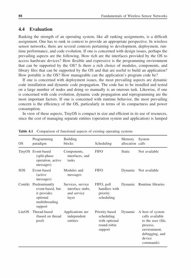
88 Fundamentals of Wireless Sensor Networks
4.4 Evaluation
Ranking the strength of an operating system, like all ranking assignments, is a difficultassignment. One has to rank in context to provide an appropriate perspective. In wirelesssensor networks, there are several contexts pertaining to development, deployment, run-time performance, and code evolution. If one is concerned with design issues, perhaps theprevailing aspects are the following. How rich are the interfaces provided by the OS toaccess hardware devices? How flexible and expressive is the programming environmentthat can be supported by the OS? Is there a rich choice of modules, components, andlibrary files that can be supported by the OS and that are useful to build an application?How portable is the OS? How manageable can the application’s program code be?
If one is concerned with deployment issues, the most prevailing aspects are dynamiccode installation and dynamic code propagation. The code has to be installed and testedon a large number of nodes and doing so manually is an onerous task. Likewise, if oneis concerned with code evolution, dynamic code propagation and reprogramming are themost important factors. If one is concerned with runtime behavior, the most prevailingconcern is the efficiency of the OS, particularly in terms of its compactness and powerconsumption.
In view of these aspects, TinyOS is compact in size and efficient in its use of resources,since the cost of managing separate entities (operation system and application) is lumped
Table 4.1 Comparison of functional aspects of existing operating systems
Programming Building Memory SystemOS paradigm blocks Scheduling allocation calls
TinyOS Event-based(split-phaseoperation, activemessages)
Components,interfaces, andtasks
FIFO Static Not available
SOS Event-based(activemessages)
Modules andmessages
FIFO Dynamic Not available
Contiki Predominantlyevent-based, butit providesoptionalmultithreadingsupport
Services, serviceinterface stubs,and servicelayer
FIFO, pollhandlers withpriorityscheduling
Dynamic Runtime libraries
LiteOS Thread-based(based on threadpool)
Applications areindependententities
Priority-basedschedulingwith optionalround-robinsupport
Dynamic A host of systemcalls availableto the user (file,process,environment,debugging, anddevicecommands)

Operating Systems 89
into a single assignment of managing a monolithic binary. But replacement or repro-gramming cost is high. SOS, Contiki, and LiteOS provide flexible support for dynamicreprogramming and hence are well suited to applications which potentially undergo inten-sive updating and upgrading processes. However, the cost of image propagation shouldnot be underestimated. LiteOS’s approach of viewing the network as a distributed filesystem is interesting, since it provides the user an intuitive way of navigating the net-work. However, since nodes are stateless and all update history should be stored at theuser’s side, it results in extra traffic in the network to disseminate commands and stateinformation.
Generally, the field of wireless sensor networks is relatively young. The operationenvironments as well as the application requirements are likely to evolve and to bemade more compact and refined. Subsequently, the tradeoff is between dynamic repro-gramming and code replacement on the one hand, and code execution efficiency onthe other.
Tables 4.1 and 4.2 provide summaries of the functional and nonfunctional aspects ofthe four operating systems presented in this chapter.
Table 4.2 Comparison of nonfunctional aspects of existing operating systems
Minimum system Separation of DynamicOS overhead concern reprogramming Portability
TinyOS 332 bytes There is no clean distinctionbetween the OS and theapplication. Atcompilation time aparticular configurationproduces a monolithic,executable code.
Requires externalsoftware support
High
SOS ca. 1163 bytes Replaceable modules arecompiled to produce anexecutable code. There isno clean distinctionbetween the OS and theapplication.
Supported Medium to low
Contiki ca. 810 bytes Modules are compiled toproduce areprogrammable andexecutable code, but thereis no separation ofconcern between theapplication and the OS.
Supported Medium
LiteOS Not available Applications are separateentities; they aredeveloped independent ofthe OS.
Supported Low

90 Fundamentals of Wireless Sensor Networks
Exercises
4.1 What is a process in the context of operating systems?
4.2 What is intra-process communication and how does it differ from inter-processcommunication?
4.3 Explain the difference between a system program and an application program?
4.4 What are system calls?
4.5 Explain the following terms and what are some of the mechanisms to avoid them?
(a) race condition(b) deadlock(c) starvation
4.6 Compare the following scheduling mechanisms:
(a) FIFO scheduling(b) sorted queue(c) round-robin
4.7 What are interrupts and interrupt handlers?
4.8 Why do most operating systems in WSNs define a kernel?
4.9 What is a preemptive process? Provide an example.
4.10 How is concurrency supported in TinyOS?
4.11 What is split-phase programming and how is it useful in WSNs?
4.12 Explain the difference between configuration components and modules in TinyOS.
4.13 Why do threads require their own separate stacks and what is the problem with thisapproach in WSNs?
4.14 Give three reasons for supporting dynamic reprogramming in WSNs.
4.15 Explain the difference between event-based and thread-based operating systems.Discuss some of the advantages and disadvantages of the two approaches in thecontext of WSNs.
4.16 Explain the difference between static and dynamic memory allocation.
4.17 State how the separation of concern is supported in the following operating systems:
(a) Contiki(b) SOS(c) LiteOS
4.18 Explain the following concepts in TinyOS:
(a) commands(b) tasks(c) events

Operating Systems 91
4.19 What is the difference between a TinyOS command and a SOS message?
4.20 Why is the state of a module stored in a separate memory space (outside of themodule) in SOS?
4.21 Explain how SOS supports dynamic reprogramming.
4.22 How is multithreading supported in a Contiki environment?
4.23 What is the function of a program loader in Contiki and why is it important?
4.24 How is module replacement supported in Contiki?
4.25 What is the advantage of considering a WSN as distributed file system in LiteOS?
4.26 What is differential patching in LiteOS?
4.27 Explain the functions of the following message handlers in SOS:
(a) init-handler(b) final-handler
4.28 State the type of scheduling strategy that the following operating systems employ:
(a) TinyOS(b) SOS(c) Contiki(d) LiteOS
4.29 How does TinyOS deal with dynamic reprogramming?
4.30 Why is separation of concern in TinyOS not a priority?
References2.x Working Group TT (2005) Tinyos 2.0. SenSys ’05: Proceedings of the 3rd International Conference on
Embedded Networked Sensor Systems (p. 320). ACM, New York, NY, USA.Cao, Q., Abdelzaher, T., Stankovic, J., and He, T. (2008) The LiteOS operating system: Towards Unix-
like abstractions for wireless sensor networks. IPSN ’08: Proceedings of the 7th International Confer-ence on Information Processing in Sensor Networks (pp. 233–244). IEEE Computer Society, Washington,DC, USA.
Cao, Q., and Abdelzaher, T. (2006) LiteOS: A lightweight operating system for C++ software developmentin sensor networks. SenSys ’06: Proceedings of the 4th International Conference on Embedded NetworkedSensor Systems (pp. 361–362). ACM, New York, NY, USA.
Dunkels, A., Gronvall, B., and Voigt, T. (2004) Contiki: A lightweight and flexible operating system fortiny networked sensors. LCN ’04: Proceedings of the 29th Annual IEEE International Conference on LocalComputer Networks (pp. 455–462). IEEE Computer Society, Washington, DC, USA.
Dunkels, A., Schmidt, O., Voigt, T., and Ali, M. (2006) Protothreads: Simplifying event-driven programmingof memory-constrained embedded systems. Proceedings of the 4th International Conference on EmbeddedNetworked Sensor Systems (SenSys), Boulder, CO. SenSys ’06. ACM, New York, NY, USA (pp. 29–42).
Gay, D., Levis, P., and Culler, D. (2007) Software design patterns for TinyOS. ACM Trans. Embed. Comput.Syst . 6 (4), 22.
Han, C.C., Kumar, R., Shea, R., Kohler, E., and Srivastava, M. (2005) A dynamic operating system for sensornodes. MobiSys ’05: Proceedings of the 3rd International Conference on Mobile Systems, Applications, andServices (pp. 163–176). ACM, New York, NY, USA.
Hill, J., Szewczyk, R., Woo, A., Hollar, S., Culler, D., and Pister, K. (2000) System architecture directions fornetworked sensors. ASPLOSIX: Proceedings of the 9th International Conference on Architectural Supportfor Programming Languages and Operating Systems (pp. 93–104). ACM, New York, NY, USA.


Part TwoBasic ArchitecturalFramework


5Physical LayerOne of the desirable aspects of wireless sensor nodes is their ability to communicate over awireless link. Because of it, mobile applications can be supported; flexible deployment ofnodes is possible; and the nodes can be placed in areas that are otherwise inaccessible towired nodes. Once the deployment is carried out, it is possible to rearrange node placementin order to attain optimal coverage and connectivity; and the rearrangement can be madewithout disrupting the normal operation of the structure or process the nodes monitor.
However, wireless communication poses some formidable challenges. Some of thesechallenges are limited bandwidth, limited transmission range, and poor packet delivery per-formance because of interference, attenuation, and multipath scattering. In order to tacklethese challenges, it is vital to understand their properties and some of the mitigation strate-gies that are already in place.
This chapter provides a fundamental introduction to point-to-point wireless digital com-munication.
5.1 Basic Components
The basic components of a digital communication system are the transmitter, the channel,and the receiver. Since wireless sensor nodes are placed close to each other in a wirelesssensor network, here short range communication is of interest. For a more comprehensivetreatment of wireless and digital communications, the reader is referred to Proakis (2000)and Wilson (1995).
Figure 5.1 provides a block diagram of a digital communication system. The commu-nication source in the context of this book represents one or more sensors and producesa message signal, an analog signal. The signal is a baseband signal having dominant fre-quency components near zero. The message signal has to be converted to a discrete signal(discrete both in time and amplitude) in order to be processed by the processor subsystem.The conversion requires sampling the signal at least at Nyquist rate,1 so that no informationwill be lost. After sampling, the discrete signal is converted to a binary stream. This processis called source encoding . It is essential to implement an efficient source-coding techniqueso that the channel’s bandwidth and signal power requirements are satisfied. One way to
1 For a band-limited signal, the Nyquist rate sets a lower bound on the sampling frequency. Hence, the minimumsampling rate should be twice the bandwidth of the signal.
Fundamentals of Wireless Sensor Networks: Theory and Practice Waltenegus Dargie and Christian Poellabauer 2010 John Wiley & Sons, Ltd
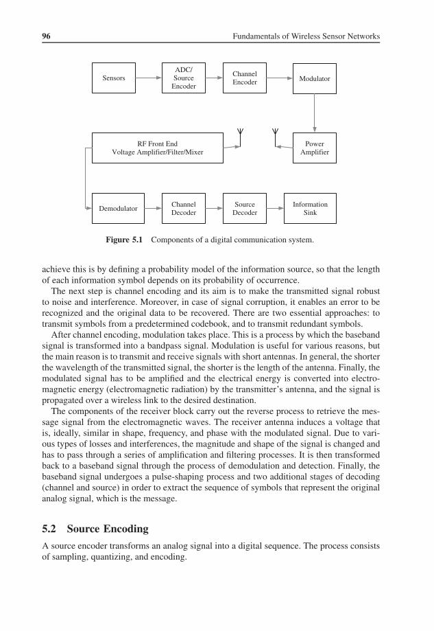
96 Fundamentals of Wireless Sensor Networks
SensorsADC/Source
Encoder
ChannelEncoder Modulator
RF Front EndVoltage Amplifier/Filter/Mixer
DemodulatorChannelDecoder
SourceDecoder
InformationSink
PowerAmplifier
Figure 5.1 Components of a digital communication system.
achieve this is by defining a probability model of the information source, so that the lengthof each information symbol depends on its probability of occurrence.
The next step is channel encoding and its aim is to make the transmitted signal robustto noise and interference. Moreover, in case of signal corruption, it enables an error to berecognized and the original data to be recovered. There are two essential approaches: totransmit symbols from a predetermined codebook, and to transmit redundant symbols.
After channel encoding, modulation takes place. This is a process by which the basebandsignal is transformed into a bandpass signal. Modulation is useful for various reasons, butthe main reason is to transmit and receive signals with short antennas. In general, the shorterthe wavelength of the transmitted signal, the shorter is the length of the antenna. Finally, themodulated signal has to be amplified and the electrical energy is converted into electro-magnetic energy (electromagnetic radiation) by the transmitter’s antenna, and the signal ispropagated over a wireless link to the desired destination.
The components of the receiver block carry out the reverse process to retrieve the mes-sage signal from the electromagnetic waves. The receiver antenna induces a voltage thatis, ideally, similar in shape, frequency, and phase with the modulated signal. Due to vari-ous types of losses and interferences, the magnitude and shape of the signal is changed andhas to pass through a series of amplification and filtering processes. It is then transformedback to a baseband signal through the process of demodulation and detection. Finally, thebaseband signal undergoes a pulse-shaping process and two additional stages of decoding(channel and source) in order to extract the sequence of symbols that represent the originalanalog signal, which is the message.
5.2 Source Encoding
A source encoder transforms an analog signal into a digital sequence. The process consistsof sampling, quantizing, and encoding.

Physical Layer 97
To explain these stages, suppose a sensor produces an analog signal that can be expressedas s(t). During the sampling process, s(t) will be sampled and quantized by the analog-to-digital converter (ADC) that has a resolution of Q distinct values. As a result, a sequence ofsamples, S = (s[1], s[2], ..., s[n]) are produced. The difference between the sampled s[j ]and its corresponding analog value at time tj is the quantization error. As the signal variesover time, the quantization error also varies and can be modeled as a random variable witha probability density function, Ps(t).
The aim of the source encoder is to map each quantized element, s[j ] into a correspondingbinary symbol of length r from a codebook, C. If all the binary symbols in the codebook areof equal length, the codebook is called a Block Code. Often, however, the symbol length aswell as the sampling rate is not uniform. It is customary, therefore, to assign short-sized sym-bols and high sampling rates to the most probable sample values and long-sized symbols andlow sampling rates to less probable sample values. Figure 5.2 illustrates the input–outputrelationship of a source encoder.
A codebook, C, can be uniquely decoded, if each sequence of symbols, (C(1), C(2), ...)
can be mapped back to a corresponding value in S = (s[1], s[2], ..., s[n]). A binary code-book has to satisfy Equation (5.1) to be uniquely decoded.
u∑i=1
(1
r
)li
≤ 1 (5.1)
where u is the size of the codebook and li is the size of the codeword C(i).A codebook can be instantaneously decoded if each symbol sequence can be extracted
(decoded) from a stream of symbols without taking into consideration previously decodedsymbols. This will be possible if and only if there does not exist a symbol in the codebook,such that the symbol a = (a1, a2, ..., am) is not a prefix of the symbol b = (b1, b2, ..., bn),where m < n and ai = bi, ∀i = 1, 2, ...,m within the same codebook. Table 5.1 lists differ-ent types of codebooks.
Source Encodera ∈A : A = q − ray c ∈C : C = M − ray
Figure 5.2 Input – output relationship of a source encoder.
Table 5.1 Source-encoding techniques
C1 C2 C3 C4 C5 C6
s1 0 00 0 0 0 0s2 10 01 100 10 01 10s3 00 10 110 110 011 110s4 01 11 11 1110 111 111
Block code No Yes No No No NoUniquely decoded No Yes No Yes Yes Yes∑n
i=1
( 12
)li 1 14 1 1 15
16 < 1 1 1Instantly decoded No Yes (block code) No Yes (comma code) No Yes

98 Fundamentals of Wireless Sensor Networks
5.2.1 The Efficiency of a Source Encoder
The efficiency of a source encoder is a quantity that expresses the average length,L(C) = E[li(C)] of symbols used to represent the sampled analog signal.
Suppose the probability of a q-ary source – that is, it has q distinct symbols – producingthe symbol si is Pi and the symbol Ci in a codebook is used to encode si . The expectedlength of the codebook is given by:
L(C) =q∑
i=1
Pi · li (C) (5.2)
Sometimes, it is necessary to express efficiency in terms of the information entropy orShannon’s entropy. In information theory, Shannon’s entropy is defined as the minimummessage length necessary to communicate information. It is related to the uncertainty asso-ciated with the information. If the symbol si can be expressed by a binary symbol of n bits,the information content of si is:
I (si) = − log2 Pi = log21
Pi
(5.3)
The entropy (in bits) of a q-ary memoryless source encoder is expressed as:
Hr(A) = E [Ir(si)] =q∑
i=1
P(si) · Ir(si) =q∑
i=1
P(si) · log21
P(si)(5.4)
The efficiency of a source encoder in terms of entropy reveals the unnecessary redundancyin the encoding process. This can be expressed by:
η(C) = H(S)
L(C)(5.5)
The redundancy of the encoder is:
L − H(S)
L= 1 − η (5.6)
5.2.1.1 Example
Suppose the analog signal in Figure 5.3 is quantized into four distinct values, 0, 1, 2, 3.As can be seen in the figure, some values (2) occur more frequently than others (0 and3). If the probability of occurrence of these values can be expressed as P(0) = 0.05,
P (1) = 0.2, P (2) = 0.7, P (3) = 0.05, then, it is possible to compute the efficiency of twoof the codebooks given in Table 5.1, namely C2 and C3.
For P1 = 0.05, log2
(1
0.05
)= 4.3. Because li has to be a whole number and there should
be no loss of information, l1 must be 5. Likewise, l2 = 3; l3 = 1; and l4 = 5. Hence:
E[L(C2)] =∑
j
lj · Pj = (5 × 0.05) + (3 × 0.2) + (1 × 0.7) + (5 × 0.05) = 1.8 (5.7)

Physical Layer 99
11
10
01
00t
Figure 5.3 An analog signal with four possible values.
Using Equation (5.4), the entropy of C2 is calculated as:
H(C2) =0.05 log2
(1
0.05
)+ 0.2 log2
(1
0.2
)
+ 0.7 log2
(1
0.7
)+ 0.05 log2
(1
0.05
)= 1.3 (5.8)
Therefore, the encoding efficiency of the codebook, C2 (see Table 5.2) is:
η(C2) = 1.3
1.8= 0.7 (5.9)
The redundancy in C2 is:
rddC2 = 1 − η = 1 − 0.67 = 0.3 (5.10)
In terms of energy efficiency, this implies that 30% of the transmitted bits are unneces-sarily redundant, because C2 is not compact enough.
In the same way lj is computed for C2, the expected symbol length (in bits) for C3 (seeTable 5.3) is given as:
E[L(C3)] =∑
j
lj · Pj
= (3 × 0.05) + (2 × 0.2) + (1 × 0.7) + (3 × 0.05)
= 1.4 (5.11)
Table 5.2 Description of the compactness of C2
j aj Pj lj
1 00 0.05 52 01 0.2 33 10 0.7 14 11 0.05 5

100 Fundamentals of Wireless Sensor Networks
Table 5.3 Description of the compactness of C3
j aj Pj lj
1 100 0.05 32 11 0.2 23 0 0.7 14 110 0.05 3
Because the probabilities of the symbols are unchanged, entropy also remains unchanged.The encoding efficiency of C3 is therefore:
η(C3) = 1.3
1.4= 0.9 (5.12)
The redundancy, rdd, in C3 is:
rddC3 = 1 − η = 1 − 0.9 = 0.1 (5.13)
5.2.2 Pulse Code Modulation and Delta Modulation
Pulse code modulation (PCM) and delta modulation (DM) are the two predominantlyemployed source encoding techniques. In digital pulse code modulation, the signal is firstquantized and then each sample is represented by a binary word from a finite set of words.The size of the individual words as well as the number of words in the set determines theresolution of a PCM technique and the source encoder bit rate.
In PCM information is conveyed in the presence or absence of pulses and not in theamplitude or the location of the edges of the pulses. Because of this property, PCM greatlyenhances (almost noise free) the transmission and regeneration of binary words. The asso-ciated cost with this form of source encoding is the quantization error and the energy andbandwidth required to transmit multiple bits for each sampled output. Figure 5.4 illustratesa PCM technique that uses two bits to encode a single sample. Four distinct levels are per-missible during sampling.
Delta modulation is a digital pulse modulation technique which has found widespreadacceptance in low bit rate digital systems. It is a differential encoder and transmits bits ofinformation which describes the difference between successive signal values, as opposedto the actual values of a time-series sequence. The difference signal, Vd(t), is produced byfirst estimating the signal’s magnitude based on previous samples (Vi(t0)) and comparingthis value with the actual input signal, Vin(t0). The polarity of the difference value indicatesthe polarity of the pulse transmitted. The difference signal is a measure of the slope of thesignal, which can be achieved by first sampling the analog signal and then by varying theamplitude, width, or the position of the digital signal in accordance with the amplitude ofthe sampled signal. Figure 5.5 illustrates delta modulation.

Physical Layer 101
11 11 101001
T 2T 3T 4T (n−1)T nT t
t
A(t)
Figure 5.4 A PCM based source encoding.
A(t)
t
Figure 5.5 Delta encoding.
5.3 Channel Encoding
The main purpose of a channel encoder is to produce a sequence of data that is robust tonoise and to provide error detection and forward error correction mechanisms. In simpleand cheap transceivers, forward error correction is costly and, therefore, the task of channelencoding is limited to the detection of errors in packet transmission.
The physical channel sets limits to the magnitude and the rate of signal transmission.Figure 5.6 illustrates these restrictions. According to the Shannon–Hartley theorem, the
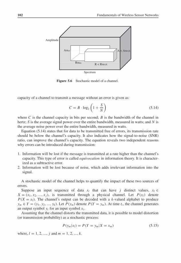
102 Fundamentals of Wireless Sensor Networks
Amplitude
Spectrum
AMax
RMax R < RMAX
A < AMAX
Figure 5.6 Stochastic model of a channel.
capacity of a channel to transmit a message without an error is given as:
C = B · log2
(1 + S
N
)(5.14)
where C is the channel capacity in bits per second; B is the bandwidth of the channel inhertz; S is the average signal power over the entire bandwidth, measured in watts; and N isthe average noise power over the entire bandwidth, measured in watts.
Equation (5.14) states that for data to be transmitted free of errors, its transmission rateshould be below the channel’s capacity. It also indicates how the signal-to-noise (SNR)ratio, can improve the channel’s capacity. The equation reveals two independent reasonswhy errors can be introduced during transmission:
1. Information will be lost if the message is transmitted at a rate higher than the channel’scapacity. This type of error is called equivocation in information theory. It is character-ized as a subtractive error.
2. Information will be lost because of noise, which adds irrelevant information into thesignal.
A stochastic model of the channel helps to quantify the impact of these two sources oferrors.
Suppose an input sequence of data xl that can have j distinct values, xl ∈X = (x1, x2, ..., xj ), is transmitted through a physical channel. Let P(xl) denoteP(X = xl). The channel’s output can be decoded with a k-valued alphabet to produceym ∈ Y = (y1, y2, ..., yk). Let P(ym) denote P(Y = ym). At time ti , the channel generatesan output symbol yi for an input symbol xi .
Assuming that the channel distorts the transmitted data, it is possible to model distortion(or transmission probability) as a stochastic process:
P(ym|xl) = P(Y = ym|X = xm) (5.15)
where, l = 1, 2, ..., j and m = 1, 2, ..., k.

Physical Layer 103
In the subsequent analysis of the stochastic characteristic of the channel, the followingassumptions hold:
• The channel is discrete, namely, X and Y have finite sets of symbols.• The channel is stationary, namely, P(ym|xl) are independent of the time instance, i.• The channel is memoryless, namely, P(ym|xl) are independent of previous inputs and
outputs.
One way of describing transmission distortion is by using a channel matrix, PC .
PC =
P(y1|x1) ... P (yk|x1)...
...
P (y1|xj ) ... P (yk|xj )
(5.16)
where
k∑m=1
p(ym|xj ) = 1 ∀j (5.17)
Moreover:
P(ym) =j∑
l = 1P(ym|xl).P (xl) (5.18)
or, more generally:
(→Py) = (
→Px) · [PC] (5.19)
where both (→Py) and
→Px are row matrices.
5.3.1 Types of Channels
5.3.1.1 Binary Symmetric Channel
A binary symmetric channel (BSC) is a channel model through which bits of information(0 and 1) can be transmitted. The channel transmits a bit of information correctly (regardlessof whether 0 or 1 is transmitted) with a probability p and incorrectly (by flipping 1 to 0 and0 to 1) with a probability 1 − p. Such a model is displayed in Figure 5.7.
The conditional probabilities for correct and incorrect transmissions are given as:
P(y0|x0) = P(y1|x1) = 1 − p (5.20)
P(y1|x0) = P(y0|x1) = p (5.21)
The channel matrix of a binary symmetric channel is, therefore given as:
PBSC =[
(1 − p) p
p (1 − p)
](5.22)

104 Fundamentals of Wireless Sensor Networks
X = 0 Y = 0
X = 1 Y = 1
1−p
1−p
p
p
Figure 5.7 A binary symmetric channel model.
X = 0
X = y
Y = 0
Y = e
Y = 1
1– p
1– p
p
p
Figure 5.8 A stochastic model of a binary erasure channel.
5.3.1.2 Binary Erasure Channel
In a binary erasure channel (BEC), there is no guarantee that the transmitted bit of informa-tion can be received at all (correctly or otherwise). Therefore the channel is characterized asa binary input and a ternary output channel. The probability of erasure is p and the probabil-ity that the information is correctly received is 1 − p. In an erasure channel the probabilityof error is zero. Figure 5.8 illustrates a binary erasure channel.
The channel matrix for a binary erasure channel is given as:
PBEC =[
(1 − p) p 00 p (1 − p)
](5.23)
Equation (5.23) states that a bit of information is either transmitted successfully withP(1|1) = P(0|0) = 1 − p or is erased altogether by the channel with a probability of p.The probability that 0 is received by transmitting 1 or vice versa is 0.
5.3.2 Information Transmission over a Channel
Given the input message, X : (X,Px→,H(X)), the channel matrix, [PC] and the output mes-
sage, Y : (Y,Py→, H(Y )), it is possible to describe the impact of irrelevance and equivocation
as well as the percentage of information that can be transmitted over the channel without anerror, which is also called transinformation or mutual information.
5.3.2.1 Irrelevance
The content of information that can be introduced into the channel due to noise isdescribed as the conditional information content, I (y|x). It is the information content

Physical Layer 105
of y that can be observed provided that x is known. The conditional entropy isgiven as:
H(y|x) = Ey[I (y|x)] =∑y∈Y
P (y|x) · log2
(1
P(y|x)
)(5.24)
P(y|x) can be known from the channel matrix [PC]. The average conditional entropyover all input message symbols, x ∈ X, is given by:
H(Y |X) = Ex[H(Y |x)] =∑x∈X
P (x) ·∑y∈Y
P (y|x) · log2
(1
P(y|x)
)(5.25)
which is also equal to:
H(Y |X) = Ex[H(Y |x)] =∑x∈X
∑y∈Y
P (y|x) · P(x) · log2
(1
P(y|x)
)(5.26)
From Baye’s law, it is clear that:
p(x, y) = P(y|x) · P(x) (5.27)
According to Equation (5.26), a good channel encoder is one that reduces the irrelevanceentropy.
5.3.2.2 Equivocation
The content of information that can be lost because of the channel’s inherent constraints canbe quantified by observing the input x given that the output y is known:
H(X|Y ) =∑x∈X
∑y∈Y
P (x|y) · P(y) · log2
(1
P(x|y)
)(5.28)
Once again, applying Baye’s conditional probability:
P(x|y) = P(y|x) · P(x)
P (y)= P(y|x) · p(x)∑
x∈X P (y|x) · P(x)(5.29)
The conditional probability of Equation (5.29) is also known as the probability of infer-ence or posterior probability. Therefore, equivocation is sometimes called inference entropy.A good channel encoding scheme is one that has a high inference probability. This can beachieved by introducing redundancy during channel encoding.
5.3.2.3 Transinformation
The information content I (X; Y ) that overcomes the channel’s constraints to reach thedestination (the receiver) is called transinformation. Given the input entropy, H(X), andequivocation, H(X|Y ), the transinformation is computed as:
I (X; Y ) = H(X) − H(X|Y ) (5.30)

106 Fundamentals of Wireless Sensor Networks
I(E) I(D)
E I(E, D) N
Figure 5.9 Irrelevance, equivocation, and transinformation.
Expanding Equation (5.30) yields:∑x∈X
P (x) · log2
(1
P(x)
)−∑x∈X
∑y∈Y
P (x, y) · log2
(1
P(x|y)
)(5.31)
Rearranging the terms in Equation (5.31) also yields:
H(Y ) − H(Y |X) = I (Y ;X) (5.32)
Irrelevance, equivocation, and transinformation, are summarized in Figure 5.9.
5.3.3 Error Recognition and Correction
Apart from improving the transinformation of a channel, it is also essential to recognizeand correct errors during transmission. Error recognition can be achieved by permittingthe transmitter to transmit only specific types of words. If a channel decoder recognizesunknown words, it attempts to correct the error or requests for retransmission (known asautomatic repeat request, ARQ). In principle, a decoder can correct only m number of errors,where m depends on the size of the word. Error correction, or more precisely, forward errorcorrection, can be achieved by sending n bits of information together with r control bits.The problem with forward error correction is that it slows down transmission.
5.4 Modulation
Modulation is a process by which the characteristics (amplitude, frequency, and phase) ofa carrier signal are modified according to the message (a baseband) signal. Modulation hasseveral advantages:
• the message signal will become resilient to noise;• the channel’s spectrum can be used efficiently; and• signal detection will be simple.
5.4.1 Modulation Types
The message signal is a baseband signal. That means, its dominant frequency componentsare in the vicinity of zero. If this signal were to be transmitted over a wireless link with-out any form of modulation, one would need a receiver antenna whose size should be

Physical Layer 107
approximately equal to one-fourth of the size of the signal’s wavelength. This is very longand it is impractical to deploy such an antenna on wireless devices.
The alternative is to superimpose the message signal on a bandpass carrier signal whosewavelength is very much smaller than the baseband signal. Due to several practical reasons,sinusoidal carrier signals are used for modulation. The properties of a sinusoidal carriersignal can be described by Equation (5.33).
sc(t) = SC sin(2πf t + φ(t)) (5.33)
where SC is the peak amplitude of the signal; f is the frequency; and φ(t) is the phase(relative position of the signal with respect to a reference signal). A radio frequency signalcan also be described in terms of its wavelength, which is a function of the propagation speedand the frequency. Figure 5.10 shows two sinusoidal signals that have the same frequencyand amplitude, but are also out of phase by φ degrees.
It is also customary to use polar presentation to describe the relationship between twosinusoidal signals that have the same frequency. Figure 5.11 illustrates the relationshipbetween the two sinusoidal signals shown in Figure 5.10.
A message signal, sm(t), can change either the amplitude, the phase, or frequency ofsc(t). If sm(t) changes the amplitude of sc(t), the modulation is known as amplitude modu-lation (AM). If sm(t) changes the frequency of sc(t), the modulation is known as frequencymodulation (FM). If sm(t) changes the phase of sc(t), the modulation is known as phase mod-ulation. Likewise, sm(t) can be a digital (binary) signal, in which case, the correspondingmodulation types are called, amplitude shift keying (ASK), frequency shift keying (FSK),and phase shift keying (PSK).
A modulation process can further be classified into coherent or noncoherent; binary or q-ary; and power-efficient or spectrum-efficient. In a coherent modulation technique a carriersignal of the same frequency (and ideally, of the same phase) is required to demodulate(detect) the received signal. In a noncoherent modulation technique, no additional carriersignal is required to demodulate the received signal. In a binary modulation, the modulating(message) signal is binary, whereas in a q-ary modulation, the modulating signal can have m
discrete values. In a power-efficient modulation technique, the aim is to optimize the powerof the modulated signal, whereas in a spectrum-efficient modulation technique, the aim isto optimize the bandwidth of the modulated signal.
A
t
j
Figure 5.10 Two signals having a phase difference of φ.

108 Fundamentals of Wireless Sensor Networks
Im
Sc2
Sc1 Re
j
Figure 5.11 Representation of a relationship between signals with a polar diagram.
5.4.1.1 Amplitude Modulation
Considering that both the carrier and the modulating signals are analog sinusoidal signals,an amplitude modulation can mathematically be described as follows:
smod(t) = [SC × SM cos (2πfmt + φm)] cos (2πfct + φc) (5.34)
In other words, the amplitude of sc(t) is varied according to the modulating signal, sm(t).To simplify the analysis, assume that the two signals are in phase (φm = φc = 0) and thus,Equation (5.34) reduces to:
smod(t) = [SC × SM cos (2πfmt)] cos (2πfct) (5.35)
Applying Euler’s formula (ejωt = cos(ωt) + j sin(ωt)), Equation (5.35) reduces to:
smod(t) = SC × SM
2[cos (2π (fc + fm) t) + cos (2π (fc − fm) t)] (5.36)
In reality, the message signal is not a mere sinusoidal signal. Instead, it is a basebandsignal that has a bandwidth of B in which the amplitude and frequency change as functionsof time. The Fourier transformation of such a baseband signal resembles that displayed inFigure 5.12. The Fourier transformation of the carrier signal is displayed in Figure 5.13.Hence, the spectrum of the amplitude modulated signal based on Figure 5.12 and Figure 5.13looks like the one displayed in Figure 5.14.

Physical Layer 109
M ( f )
M (0)
−fm fm f02B
Figure 5.12 The spectrum of a baseband signal having a bandwidth of B.
M ( f )
−fc 0 ffc
Sc2
Sc2
Figure 5.13 The Fourier transformation of a carrier signal having a frequency of fc.
M ( f )
− fc − fm − fc + fm fc − fm fc + fm
Sc
2
Sc
2
02Β 2Β
f
Figure 5.14 The Fourier transformation of an amplitude modulated signal.
Figure 5.15 illustrates the technical aspect of an amplitude modulation. The basebandsignal and the carrier signal are mixed (multiplied) by using a mixer, which is, typically, anamplifier having a bandwidth greater than the bandwidth of the baseband signal. Afterwards(not shown here) the signal passes through a number of amplification and filtering processesso that the channel’s amplitude and spectrum requirements are fulfilled.
The demodulation process – the extraction of the message signal from the modulatedsignal – is similar to the modulation process, but involves at least one additional process,that is, lowpass filtering. First, the received modulated signal is mixed (multiplied) with acarrier signal that has the same frequency and, ideally, the same phase as the original carriersignal, SC(t). Mathematically, this is expressed as:
sdemo(t) = SC cos (2πfct) × smod(t) (5.37)

110 Fundamentals of Wireless Sensor Networks
Smcos(2pfmt)
Sccos(2pfct)
Smod(t)
X
Figure 5.15 Amplitude modulation.
Expanding Equation (5.37) yields:
sdemo(t) = SC cos (2πfct) × KSC × SM
2[cos (2π (fc + fm) t) + cos (2π (fc − fm) t)]
(5.38)
where K1, which signifies that the modulated signal is attenuated. Applying propertiesof trigonometry, Equation (5.38) can be simplified into:
sdemo(t) = KS2CSM
4[cos (2π (2fc − fm) t) + cos (2π (2fc + fm) t) + 2 cos (2πfmt)]
(5.39)
As can be seen, Equation (5.39) contains the message signal and a carrier signal whosefrequency is much higher than the message signal. The two components can very easilybe separated by using a simple envelope detector consisting of a half-wave rectifier anda lowpass filter. Figure 5.16 shows how a modulated signal is mixed with a carrier signalgenerated by the local oscillator of the receiver. The result passes through a bandpass filter(not shown here) to remove the fc component. Afterwards, a simple half-wave rectifier anda lowpass filter are used to retrieve the message (baseband) signal.
Sccos(2pfc t)
Smcos(2pfmt)
Smod(t)
X Rectifier Low-passfilter
Figure 5.16 Demodulating an AM carrier signal.

Physical Layer 111
5.4.1.2 Frequency and Phase Modulation
In frequency modulation, the amplitude of the carrier signal, sc(t), remains intact, but itsfrequency changes according to the message signal, sm(t). Here, it is essential to restrict theamplitude of the modulating signal such that |sm(t)| ≤ 1. Hence, the modulated signal isdescribed as follows:
sFM(t) = SC cos
(2π
∫ t
0f (τ) dτ
)(5.40)
where∫ t
0 f (τ)dτ is the instantaneous variation of the local oscillator’s frequency. Express-ing this frequency variation as a function of the modulating signal yields:
sFM(t) = SC cos
(2π
∫ t
0[fc + fδsm(τ)] dτ
)(5.41)
where fδ is the maximum frequency deviation of the carrier frequency, fc. Rearranging theterms in Equation (5.41) yields:
sFM(t) = SC cos
(2πfct + 2πfδ
∫ t
0sm(τ)dτ
)(5.42)
In phase modulation, the phase of the carrier changes in accordance with the messagesignal.
5.4.1.3 Amplitude Shift Keying
So far, the modulated signal was considered to be analog. In digital communication, themodulated signal is a binary stream.
Amplitude shift keying is a digital modulation technique in which the amplitude of ananalog carrier signal is varied in accordance with a binary stream. The frequency and phaseof the carrier signal remain unchanged.
There are several possibilities to realize amplitude shift keying. The simplest is to use anon–off modulation system, as shown in Figure 5.17. Accordingly to Figure 5.17, the mixer(multiplier) produces an output that is the multiplication of the two input signals – one ofwhich is the message stream and the other is the output of the local oscillator, namely, thesinusoidal carrier signal having a frequency of fc.
Direct mixing a square wave (the bit stream) requires a mixer with an excessive band-width, which is expensive to afford. Alternatively, an amplitude shift keying can take placeby using a pulse-shaping filter (PSF). The PSF removes high-frequency components from
X
cos(2pfct)
Figure 5.17 Amplitude shift-keying technique using an on-off switch.

112 Fundamentals of Wireless Sensor Networks
cos(2pfct)
X
Figure 5.18 An amplitude shift-keying process using a pulse-shaping filter.
the square wave signal and approximates it with a low-frequency signal, which will thenmodulate the carrier signal. This is displayed in Figure 5.18.
The demodulation process employs a mixer, a local oscillator, a PSF, and a compara-tor. The mixer and the PSF are used to remove the high-frequency component from themodulated signal. The comparator changes the analog wave form into a stream of bits.
5.4.1.4 Frequency Shift Keying
In frequency shift keying, the frequency of a carrier signal changes in accordance withthe message bit stream. Since the message bit stream will have either 0 or 1, the carrierfrequency also changes between two values. Figure 5.19 demonstrates how a simple switch-ing amplifier and two local oscillators with carrier frequencies f1 and f2 can be used infrequency shift-keying modulation. The switching amplifier is controlled by the messagebit stream.
The demodulation process requires two local oscillators (with frequency f1 and f2), twoPSFs, and a comparator, as illustrated in Figure 5.20.
5.4.1.5 Phase Shift Keying
In phase shift keying the phase of a carrier signal is changed according to the message bitstream. The simplest form of phase shift keying is to make a phase shift of 180◦ whenthe bit stream changes from 1 to 0 or vice versa. Figure 5.21 shows a phase shift-keying
f1
f2
cos(2pfct)
Figure 5.19 A frequency shift-keying modulation.

Physical Layer 113
cos(2pf1t)
cos(2pf2t)
f1
f2
X
X
Figure 5.20 Demodulation in a frequency shift-keying process.
cos(2pfct)
Figure 5.21 A phase shift-keying modulation process.
process in which a transition from 1 to 0 results in a phase shift of 180◦. The modulationprocess requires a local oscillator, an inverter, a switching amplifier, and a PSF. The inverteris responsible for inverting the carrier signal by 180◦.
Alternatively, a PSF, a mixer, and a local oscillator can be used as shown in Figure 5.22.The demodulation process uses a local oscillator, a mixer, a PSF, and a comparator, as shownin Figure 5.23.
X
cos(2pfct)
Figure 5.22 A phase shift-keying modulation with a PSF.

114 Fundamentals of Wireless Sensor Networks
cos (2pfct)
X
Figure 5.23 A demodulation scheme for a phase shift keying.
5.4.2 Quadratic Amplitude Modulation
So far a single message source is used to modulate a single carrier signal. This, however,is not efficient enough. One can employ orthogonal signals to effectively exploit the chan-nel’s bandwidth. In the QAM process (Figure 5.24), two amplitude-modulated, orthogonalcarriers are combined as a composite signal, thereby achieving double bandwidth efficiencycompared to the normal amplitude modulation. QAM is used with pulse amplitude mod-ulation (PAM) in digital systems, especially in wireless applications. The modulated bitstream is divided into two parallel substreams each of which independently modulates thetwo orthogonal carrier signals.
The carrier signals have the same frequency, fc, but they are out of phase by 90◦. Sincethe signals are orthogonal, they do not interfere with each other. One of the carriers is calledthe I carrier (in-phase signal) and the other is called the Q signal (quadrature signal).
Recall that:
sQ(t) = SC cos(2πf t + 90◦) = SC sin(2πf t) (5.43)
At the receiver side, the composite modulated signal bearing the magnitude and phaseinformation of the Q and I signals will be mixed with two demodulating signals which are
QX
XI
+
90°sin(2pfct)
cos(2pfct)
Figure 5.24 A quadratic amplitude modulation process.

Physical Layer 115
identical in frequency but out of phase with each other by 90◦. Then the usual detectionprocedure carries on to extract and aggregate (mix) the message.
Figure 5.25 shows the demodulation process of a QAM signal. The composite signal withmagnitude and phase (or I and Q) information arrives at the receiver. The input signal ismixed with the carrier signal from the local oscillator in two forms. One has a referencezero phase while the other has a 90◦ phase shift. The composite input signal (in terms ofmagnitude and phase) is thus split into an in-phase, I , and a quadrature, Q, component.These two components of the signal are independent and orthogonal. One can be changedwithout affecting the other.
Digital modulation is easy to accomplish with I/Q modulators, which map the data to anumber of discrete points on the I/Q plane. These are known as constellation points. Asthe modulated signal moves from one point to another, simultaneous amplitude and phasemodulation take place. To accomplish this with an amplitude modulator and a phase mod-ulator is difficult and complex. Simultaneous amplitude and phase modulation can easilybe achieved with an I/Q modulator. The I and Q control signals are bounded, but infinitephase wrap is possible by properly phasing the I and Q signals.
5.4.2.1 Modulation Efficiency
Depending on the modulation type for each substream, the relative amplitude, phase, orfrequency of the modulated signal carries part of the message bit stream. The modulationefficiency refers to the number of bits of information that can be conveyed in a single sym-bol. In a QAM, the composite carrier signal contains two orthogonal signals. The amplitudeand phase of these signals are modified according to the message bit stream. Inasmuchas a receiver is sensitive enough to detect the relative differences in magnitude and phasebetween these two signals, much information can be conveyed with a single state of the com-posite carrier signal. However, there is a tradeoff between the compactness of the modulatedtechnique and the receiver’s complexity.
To evaluate the efficiency of a modulation technique, it is important to distinguish betweensymbol rate and bit rate. Bit rate refers to the frequency of a system’s bit stream. A symbolrate, also referred to as a baud rate, refers to the bit rate divided by the number of bits that can
Q
sin(2pfct)
cos(2pfct)
90°
I
X
X
Figure 5.25 Demodulating a QAM signal.

116 Fundamentals of Wireless Sensor Networks
01 00
10 11
Figure 5.26 Binary phase shift keying: 2 bits per symbol.
be transmitted with each symbol. For example, a 10-bit ADC that samples an accelerometersensor at a rate of 1 kHz has a bit stream of 10 bits multiplied by 1 kHz samples per second,or 10 kbps.
Now consider a quadrature phase shift keying (QPSK) digital modulation, in which aphase difference of 90◦ between the I and Q carrier signals indicates a message of 1 or 0.As can be seen in Figure 5.26, four distinct states of the composite carrier signal can bediscriminated by the demodulator. Since the message signal is in binary form, the four statescan be represented by two bits: 00, 01, 10, 11. Subsequently, the symbol rate is half of thebit rate. For the ADC example, the symbol rate is 5 kbps.
In an eight-state phase shift keying modulation, the phase of the composite carrier signalcan have eight distinct states which can be mapped into eight distinct symbols by the demod-ulator. Since the eight symbols can be represented by 3 bits, the symbol rate is one-third ofthe bit rate. In other words, the spectrum required by an eight-state phase shift keying isone-third of the spectrum required by a binary phase shift keying modulator. However, theefficiency in spectrum is achieved at the cost of complex system design. Unlike the QPSKmodulator, the 8PSK modulator (Figure 5.27) should be able to discriminate eight differenttransitions in phase of the composite carrier signal.
010 001
000
111
110101
100
011
Figure 5.27 8PSK modulation with 3 bits per symbol.

Physical Layer 117
5.4.3 Summary
The choice of a modulation technique depends on the design goals of the communicationsubsystem. There is a tradeoff between power consumption, spectrum efficiency, and cost. Apower efficient modulator enables a communication system to reliably transmit informationat the lowest practical power cost. A spectrally efficient modulator enables a communicationsubsystem to send as many bits of information as possible within a limited bandwidth. Powerand spectrum efficiency cannot be achieved at the same time.
For terrestrial links, such as microwave radios, the concern is bandwidth efficiency withlow bit-error-rate. Since sufficient power is available, power efficiency is not a concern.Moreover, for such types of links, the receiver’s cost or complexity are not usually priorconcerns. In wireless sensor networks, power efficiency is a major concern while bandwidthis not, as the nodes produce small-volume data. The cost of the transceivers is also of primeconcern in large-scale deployments. Subsequently, the communication subsystems sacrificebandwidth efficiency to achieve power and cost efficiency.
5.5 Signal Propagation
Wireless sensor networks operate in the license-free ISM spectrum (see Table 5.4) and there-fore, they must share the spectrum with and accept interference from devices that operate inthe same spectrum – such as cordless phones, WLAN, Bluetooth, Microwave ovens, etc.
A simple channel model (Figure 5.28) ignores the effect of interference and considers thesurrounding noise as the predominant factor that affects the transmitted signal. Furthermore,the noise can be modeled as an additive white Gaussian noise (AWGN) that has a constantspectral density over the entire operating spectrum and a normal amplitude distribution. Inthis model, the noise distorts the amplitude of the transmitted signal.
There are two approaches to deal with noise. First, one can increase the received power sothat the signal-to-noise ratio is significantly high and the channel becomes agnostic to noise.
Table 5.4 The Industry, Scientific and Medical (ISM) spectrum as defined by the ITU-R
Spectrum Center frequency Availability
6.765–6.795 MHz 6.780 MHz Subject to local regulations13.553–13.567 MHz 13.560 MHz26.957–27.283 MHz 27.120 MHz40.66–40.70 MHz 40.68 MHz433.05–434.79 MHz 433.92 MHz Europe, Africa, the Middle East west of the Persian
Gulf including Iraq, the former Soviet Union andMongolia
902–928 MHz 915 MHz The Americas, Greenland and some of the easternPacific Islands
2.400–2.500 GHz 2.450 GHz5.725–5.875 GHz 5.800 GHz24–24.25 GHz 24.125 GHz61–61.5 GHz 61.25 GHz Subject to local regulations122–123 GHz 122.5 GHz Subject to local regulations244–246 GHz 245 GHz Subject to local regulations

118 Fundamentals of Wireless Sensor Networks
Additive white Gaussian noise(AWGN)
Receivedsignal
Transmittedsignal
+
Figure 5.28 An additive white Gaussian noise channel.
Second, one can use a spread spectrum technique to distribute the energy of the transmittedsignal so that a wider effective bandwidth can be achieved.
The received power can be improved by adjusting a number of parameters at the side ofthe transmitter as well as the receiver. The relationship between the received power and thetransmitted power can be expressed using Figure 5.29.
Suppose the power amplifier – the final stage in the transmitter before the electric sig-nal is converted into electromagnetic waves – outputs a constant transmission power, Pt , totransmit the signal over a distance of ρ. The relationship between the transmitter’s antennagain, gt , and the antenna’s effective area, At , is expressed as:
At = gt
λ2
4π(5.44)
where λ is the wavelength of the carrier signal.At the receiver’s side, the transmitted signal will be received and the received power is a
function of the distance, the path loss index, and the receiver’s antenna gain and effectivearea. For a line-of-sight (LOS) communication link, the path loss index is 2; for a non-LOScommunication link, it lies between 2 and 4. Consequently, the relationship between thereceived power and the transmitted power for a LOS link is expressed as:
ModulationFrequencytranslation
Poweramplifier
Localoscillator
ReceiverPt
Pr
r
Figure 5.29 Relationship between the transmitted power and the received power.

Physical Layer 119
Pr = Pt
4πρ2gt × Ar (5.45)
where ρ is the distance that separates the transmitter and the receiver. Since the receiver’santenna gain, gr , and the effective area, Ar , are related, Equation (5.45) can be reformulated:
Pr = Pt
4πργgt × gr
λ2
4π(5.46)
The ratio of the transmitted power to the received power, P t/P r is the propagation lossand it is customary to quantify this ratio in decibels (dBs).
a(t) = Pt
Pr
=(
4πρ
λ
)× 1
grgt
(5.47)
Hence, the propagation loss expressed in dBs is:
a(t)/dB = 20 log
(4πρ
λ
)− 10 log (grgt ) (5.48)
The term 20 log (4πρ/λ) is called the basic transmission loss and is independent of thetransmitter and receiver antennas.
Exercises
5.1 How can a single ADC be employed by multiple sensors to convert their analog outputinto corresponding discrete sequences?
5.2 Suppose a discrete memoryless channel (DMS) source emits symbols from the ternaryalphabet A = {−1, 0, 1} with a probability, P(−1) = 0.5, P (0) = P(1) = 0.25. If thesource can also be configured such that instead of emitting one symbol at a time, it canemit two symbols (A2) with a probability that is the multiplication of the probabilitiesof the individual symbols, show that the entropy of the second configuration is twotimes greater than the entropy of the first configuration.
5.3 The following codes are given:
C1 = {1, 10, 01}C2 = {0, 00001}C3 = {0, 10, 11}C4 = {01, 11}C5 = {0, 00, 000}(a) Which of the given codes are uniquely decodable?(b) Which of the given codes are instantaneously decodable?(c) Which of the given codes can be an optimal prefix-free code for some probability
assignment?

120 Fundamentals of Wireless Sensor Networks
5.4 Suppose an information source emits symbols from an alphabet X = {x1, ..., x8} withcorresponding probabilities {0.2, 0.35, 0.15, 0.1, 0.09, 0.06, 0.04, 0.01}.(a) Calculate an upper bound on the average codeword length achievable with a binary
Shannon or Huffman code if single symbols are encoded at a time.(b) Construct a binary Huffman code for the given source.(c) Calculate the average codeword length achieved by the Huffman code and com-
pare it with the calculated bounds.
5.5 Refer to the analog signal shown in Figure 5.30.
(a) How can the signal be encoded with a 3-bit PCM?(b) How can the signal be encoded with a delta encoder?(c) Illustrate how a PCM encoder with a codebook of different symbol length can be
used to efficiently encode the signal.(d) Manchester coding is a line encoding technique that is useful for minimizing the
effect of DC voltage during data transmission and for dynamic clock recovery.Illustrate how the PCM stream can be encoded with a Manchester coding.
(e) Now instead of Manchester coding, encode the PCM stream with a differentialManchester coding.
T 2T 3T 4T (n−2)T nT t
Figure 5.30 Source coding an analog signal.
(f) Discuss the difference between the bit streams generated by the Manchester anddifferential Manchester encoding techniques.
5.6 The feedback loop shown in Figure 5.31 is a very useful concept in linear systems. Itis the basic principle for designing stable amplifiers and oscillators. Moreover, mostreceivers employ the feedback loop to set up an automatic gain control (AGC) toensure that the power of the received message signal remains constant despite changesin the channel’s properties. The feedback loop is characterized by the overall loop gain,which is the ratio of the output voltage to the input voltage, Gloop = Vout/Vin. Calculatethe overall loop gain, Gloop.
Vin
Vf
VoutG+
B
Figure 5.31 A feedback loop.

Physical Layer 121
5.7 The half-wave rectifier shown in Figure 5.32 is one of the two components of an enve-lope detector which is responsible for extracting the baseband message signal from thecarrier. Sketch the output of the rectifier for the corresponding sinusoidal input signal.
Vin
Vin
Vout
Vout
+
_
i
tt
Figure 5.32 A half-wave rectifier.
5.8 Now instead of the half-wave rectifier, the full-wave bridge rectifier shown inFigure 5.33 is used. How does the output wave form look?
Vin
Vin
Vout
Vout
+
−
t
i
t
Figure 5.33 A full-wave bridge rectifier.
5.9 A lowpass filter is required to separate the baseband signal from the carrier in an ampli-tude modulated signal. Explain how the lowpass filter shown in Figure 5.34 can be usedfor this purpose.
+
−
Vin Vout
R
C
i
Figure 5.34 An RC lowpass filter.

122 Fundamentals of Wireless Sensor Networks
Based on Figure 5.34, derive an expression for:
(a) The voltage drops across the resistor and the capacitor.(b) The current that circulates in the filter.(c) The transfer function, HC(s) = Vout(s)/Vin(s), where s = jω is the Laplace oper-
ator.
5.10 A modulating signal, m(t) = 5 cos(2π 1 kHz t), is used to amplitude modulate a car-rier signal, c(t) = 10 cos(2π 100 MHz t).
(a) Compute the time domain expression of the modulated signal.(b) Compute the frequency domain expression of the modulated signal.(c) Suppose the message signal is sampled at a period T using the Dirac delta function
as shown in Figure 5.35. What does the spectrum of the sampled signal look like?
m (t) m (nt)X
s(t) = Σ d(t − nT )∞
−∞
Figure 5.35 Sampling a modulating signal with Dirac’s delta function.
(d) What precondition should be satisfied in order to reconstruct the continuous mod-ulating signal from the sampled sequences?
5.11 The path loss index, γ , describes how an electromagnetic wave is attenuated as it prop-agates through a space. In free space, where there is no obstacle between the transmitterand the receiver, γ = 2. That means that the power of a propagating electromagneticwave falls as the function of the square of a distance – Pr ≈ Pt/4πρ2, where ρ is thedistance in meters. If, however, there is an obstacle between the transmitter and thereceiver, this figure is greater than 2. Figure 5.36 displays a simple model in whichthe electromagnetic wave reaches the receiver after being reflected once. Derive anexpression of the path loss index for the model. Assume that the reflector is an idealreflector and that there is a line-of-sight link between the transmitter and the reflectorand the receiver and the reflector. Assume also that ρ�h.
5.12 Figure 5.37 displays the block diagram of a part of a receiver. It consists of an omnidi-rectional antenna, a RF amplifier, a local oscillator, an intermediate-frequency ampli-fier, and a detector (an envelope detector). While it is possible to detect the modulatingsignal after mixing the received, modulated signal with the local carrier signal, it isuseful to have the intermediate state.
(a) Why is the intermediate frequency amplifier desirable?(b) Suppose the receiver is used for receiving an amplitude modulated signal. How
can the intermediate frequency be obtained?

Physical Layer 123
Obstacle
r
r /2 r /2
TPt Pr
R
h
Figure 5.36 Single reflection model for an electromagnetic propagation.
RF Amplifier XIF
amplifierEnvelopeDetector
Localoscillator
Figure 5.37 Block diagram of a receiver.
5.13 What type of roles do the transmitter’s and the receiver’s antennas play to enhancesignal propagation and reception?
5.14 Why is a considerable amount of power wasted at the power amplifier of a transmitter?
5.15 Explain the tradeoff between modulation efficiency and design complexity in quadra-ture amplitude modulation.
ReferencesProakis, J.G. (2000) Digital Communications (4th edn). McGraw-Hill Publishing Company.Wilson, S.G. (1995) Digital Modulation and Coding . Prentice Hall.


6Medium Access ControlIn most networks, multiple nodes share a communication medium for transmitting their datapackets. The medium access control (MAC) protocol (often referred to as a sublayer of thedata link layer of the OSI reference model) is primarily responsible for regulating access tothe common medium. Most sensor networks and sensing applications rely on radio transmis-sions in the unlicensed ISM (Industrial, Scientific, and Medical) band, which may result incommunications significantly affected by noise and interferences. The choice of MAC pro-tocol has a direct bearing on the reliability and efficiency of network transmissions due tothese errors and interferences in wireless communications and to other challenges such as thehidden-terminal and exposed-terminal problems. Other Further concerns include signal fad-ing, simultaneous medium access by multiple nodes, and asymmetric (unidirectional) links.Since energy efficiency is a primary concern in a wireless sensor network, it also affects thedesign of the MAC protocol. Energy is not only consumed for transmitting and receivingdata, but also for sensing the medium for activity (idle listening). Other reasons for energyconsumption include data retransmissions (e.g., due to collisions), packet overheads, con-trol packet transmissions, and transmit power levels that are higher than necessary to reach areceiver. It is common for a MAC protocol in WSNs to trade energy efficiency for increasedlatency or a reduction in throughput or fairness. This chapter reviews the responsibilitiesof the MAC layer in general, discusses the characteristics of MAC protocols for WSNs,describes the main classes of MAC protocols for wireless communication, and providesdescriptions of a selection of MAC protocols for WSNs.
6.1 Overview
The wireless medium must be shared by multiple network devices, therefore a mechanismis required to control access to the medium. This responsibility is carried out by the secondlayer of the OSI reference model (Figure 6.1), called the data link layer. According to theIEEE 802 reference model (also shown in Figure 6.1), this layer is further divided into thelogical link control layer and the medium access control layer. The MAC layer operatesdirectly on top of the physical layer, thereby assuming full control over the medium. Themain function of the MAC layer is to decide when a node accesses a shared medium and toresolve any potential conflicts between competing nodes. It is also responsible for correctingcommunication errors occurring at the physical layer and performing other activities suchas framing, addressing, and flow control.
Fundamentals of Wireless Sensor Networks: Theory and Practice Waltenegus Dargie and Christian Poellabauer 2010 John Wiley & Sons, Ltd

126 Fundamentals of Wireless Sensor Networks
Logical Link Control
OSI Reference Model
Application
Presentation
Session
Transport
Network
Data Link
Physical
Medium
Physical
Medium
IEEE 802Reference Model
Medium Access Control
Figure 6.1 The MAC layer in the IEEE 802 reference model.
Existing MAC protocols can be categorized by the way they control access to the medium.Figure 6.2 shows an example of such a categorization. Most MAC protocols fall either intothe categories of contention-free or contention-based protocols. In the first category, MACprotocols provide a medium sharing approach that ensures that only one device accessesthe wireless medium at any given time. This category can further be divided into fixedand dynamic assignment classes, indicating whether the slot reservations are fixed or on-demand. In contrast to contention-free techniques, contention-based protocols allow nodesto access the medium simultaneously, but provide mechanisms to reduce the number ofcollisions and to recover from such collisions. Finally, some MAC protocols do not eas-ily fit into this classification since they share characteristics of both contention-free andcontention-based techniques. These hybrid approaches often aim to inherit the advantagesof these main categories, while minimizing their weaknesses.
MACAW
Dynamic AssignmentFixed Assignment
Medium Access Control Protocol
FDMATDMACDMA
PollingToken Passing
ALOHACSMAMACA
Contention–Free Protocols Contention–Based Protocols
Reservation–Based
Figure 6.2 Categories and examples of medium access protocols.

Medium Access Control 127
6.1.1 Contention-Free Medium Access
Collisions can be avoided by allocating resources to nodes such that each node can use itsresources exclusively. For example, the frequency division multiple access (FDMA) pro-tocol is one of the oldest methods of sharing a communication medium. In FDMA, thefrequency band is divided into several smaller frequency bands, which can be used for datatransfer between a pair of nodes, while all other nodes that could potentially interfere withthis transfer use a different frequency band. Similarly, the time division multiple access(TDMA) protocol allows multiple devices to use the same frequency band, but it uses peri-odic time windows (called frames), consisting of a fixed number of transmission slots, toseparate the medium accesses of different devices. A time schedule indicates which nodemay transmit data during a certain slot, that is, each slot is assigned to at most one node.The main advantage of TDMA is that nodes do not have to contend to access the medium,thereby avoiding collisions. A downside of TDMA is that changes in the network topologynecessitate changes to the slot allocations. Further, TDMA protocols can be inefficient intheir bandwidth utilization when slots are of fixed size (and packet sizes can differ) andwhen slots allocated to a node are not used in every frame iteration. A third class of MACprotocols is based on the concept of code division multiple access (CDMA), where simul-taneous accesses of the wireless medium are supported using different codes . If these codesare orthogonal, it is possible for multiple communications to share the same frequency band,where forward error correction (FEC) at the receiver is used to recover from interferencesamong these simultaneous communications.
Fixed assignment strategies can be inefficient in that it is typically not possible to re-allocate slots belonging to one device to other devices if not needed in every frame. Also,generating schedules for an entire network (especially in large-scale wireless sensor net-works) can be a taunting task and these schedules may require modifications every timethe network topology or traffic characteristics in the network change. Therefore, dynamicassignment strategies avoid such rigid allocations by allowing nodes to access the mediumon demand. For example, in polling-based protocols, a controller device (e.g., a base stationin the case of an infrastructure-based wireless network), issues small polling frames in around-robin fashion, asking each station if it has data to send. If a station has no data tobe sent, the controller polls the next station. A variant of this approach is token passing ,where stations pass a polling request to each other (again in a round-robin fashion) usinga special frame called a token. A station is allowed to transmit data only when it holds thetoken. Finally, reservation-based protocols use static time slots to allow nodes to reservefuture access to the medium based on demand. For example, a node can indicate its desireto transmit data by toggling a reservation bit in a fixed location. These often very complexprotocols then ensure that other potentially conflicting nodes take note of such a reservationto avoid collisions.
6.1.2 Contention-Based Medium Access
In contrast to contention-free techniques, contention-based protocols allow nodes to con-tend to access the medium simultaneously, but provide mechanisms to reduce the numberof collisions and to recover from such collisions. For example, the ALOHA (Kuo 1995)protocol uses acknowledgments to confirm the success of a broadcast data transmission.

128 Fundamentals of Wireless Sensor Networks
DA B C
Figure 6.3 Hidden and exposed terminal problem.
ALOHA allows nodes to access the medium immediately, but addresses collisions withapproaches such as exponential backoff to increase the likelihood of successful transmis-sions. The slotted-ALOHA protocol tries to reduce the probability of collisions by requiringthat a station may commence transmission only at predefined points in time (the beginningof a time slot). While the slotted-ALOHA increases the efficiency of ALOHA, it also intro-duces the need for synchronization among nodes.
A popular contention-based MAC scheme is the Carrier Sense Multiple Access (CSMA)approach, including its variations Collision Detection (CSMA/CD) and Collision Avoid-ance (CSMA/CA). In CSMA/CD-based schemes, the sender first senses the medium todetermine whether it is idle or busy. If it is found busy, the sender refrains from trans-mitting packets. If the medium is idle, the sender can initiate data transmission. In wiredsystems, the sender continues to listen to the medium to detect collisions of its own datawith other transmissions. However, in wireless systems, collisions occur at the receiver, andthe sender will therefore be unaware of a collision. The hidden-terminal problem occurswhen two sender devices A and C are able to reach a receiver device B, but cannot over-hear each other’s signals (see Figure 6.3, where circles indicate transmission and interfer-ence ranges of nodes). Therefore it is possible for A and C to transmit data to B at thesame time, causing a collision at B, without being able to directly detect this collision.A related problem is the exposed-terminal problem, where C wants to transmit data to afourth node D, but decides to wait because it overhears an ongoing transmission from Bto A. However, B’s transmission will not interfere with data reception at D since D is out-side the transmission range of B. As a consequence, node C’s decision to wait delays itstransmission unnecessarily. Many MAC protocols for WSNs attempt to address these twochallenges.
6.2 Wireless MAC Protocols
A variety of wireless MAC protocols and standards are available today and this sectionprovides an overview of the most common approaches. While these protocols may notbe the best choices for wireless sensor networks, they introduce basic concepts, manyof which can be found in protocols targeted specifically at sensor networks and theirconstraints.

Medium Access Control 129
6.2.1 Carrier Sense Multiple Access
Many contention-based protocols for wireless sensor networks rely on the concept ofCSMA. The main difference between CSMA and ALOHA is that, in CSMA, nodes firstsense the medium before they begin a transmission. This reduces the number of collisions.In non-persistent CSMA, a wireless node is allowed to immediately transmit data once itfinds the medium idle. If the medium is busy, the node performs a backoff operation, thatis, it waits for a certain amount of time before attempting to transmit again. In contrast,in 1-persistent CSMA, a node wishing to transmit data continuously senses the mediumfor activity. Once the medium is found idle, the node transmits its data immediately. If acollision occurs, the node waits for a random period of time before attempting to transmitagain. In p-persistent CSMA, the node also continuously senses the medium, but transmitsdata with a probability p once the medium becomes idle and delays transmission witha probability 1 − p. Random backoff values are either continuous values in the case ofunslotted CSMA or multiples of a fixed slot size in slotted CSMA.
CSMA/CA (CSMA with Collision Avoidance) is a variation of CSMA that aims toimprove the performance by avoiding collisions. In CSMA/CA, nodes sense the medium,but do not immediately access the channel when it is found idle. Instead, a node waits for atime period called DCF interframe space (DIFS) plus the random backoff value, which is amultiple of a slot size (see Figure 6.4). In case there are multiple nodes attempting to accessthe medium, the one with the shorter backoff period will win. For example, in Figure 6.4,node A waits for DIFS + 4 × s (where s represents the slot size), while node B’s backoff isDIFS + 7 × s. Once node A begins with its transmission, node B freezes its own backofftimer and resumes the timer after node A completes its transmission plus another period ofDIFS. Finally, once node B’s backoff timer expires, it can also begin its transmission.
6.2.2 Multiple Access with Collision Avoidance (MACA) and MACAW
Other collision avoidance schemes rely on a dynamic reservation mechanism such as ready-to-send (RTS) and clear-to-send (CTS) control packets as in MACA (Karn 1990). With RTS,a sender device indicates its desire to transmit a data packet to an intended receiver. If the
Slot
TransmissionDIFS
DIFS Medium BusyMedium Busy
Medium Busy
DIFSTransmission
ContentionWindow
ContentionWindow
Node A
Node B
Figure 6.4 Medium access using CSMA/CA.

130 Fundamentals of Wireless Sensor Networks
RTS arrives without collision and the receiver is ready to receive the packet, it responds witha CTS control message. If a sender does not receive a CTS in response to its RTS, it willretry at a later time. However, if the CTS message has been received, the channel reservationhas concluded successfully. Other nodes that overhear either the RTS or CTS message knowthat a data transfer will occur, and they wait before they attempt to reserve the channel. InMACA, this wait time can be based upon the size of the data transmission, which can beindicated as part of the RTS and CTS messages. Using this handshake, MACA addressesthe hidden terminal problem and reduces the number of collisions by reserving the mediumfor data transmissions.
In MACAW (Bharghavan et al. 1994) (MACA for Wireless LANs), the receiver respondswith an acknowledgment (ACK) control message once the packet has been received cor-rectly, allowing other nodes to learn that the channel is available again and to increase thereliability of transmissions. The consequence is that nodes overhearing an RTS messagemust remain silent to ensure that the sender of the RTS is able to receive the ACK. Nodesthat overheard RTS, but did not acknowledge CTS, do not know whether they did not hearthe CTS signal because they are out of reach of the destination or because the CTS messagewas never sent. In either case, they will also not hear the ACK from the destination, that is,they must stay silent until the expected completion time of the transmission, based on theinformation carried in the RTS message. However, if no CTS was sent, they remain silentand delay their own transmission, even though no interfering transmissions are occurring.Therefore, the MACAW protocol introduces another control packet, called the data sending(DS) message. The DS message is sent by the node issuing the RTS message after receiv-ing the corresponding CTS message to confirm that a transmission will actually take place.A node overhearing an RTS message, but not the corresponding DS message, may assumethat the medium reservation has failed and can attempt to reserve the medium for its owncommunication.
6.2.3 MACA By Invitation
Another improvement is provided in the MACA By Invitation (MACA-BI) Protocol(Talucci et al. 1997), where a destination device initiates data transfers by sending a ReadyTo Receive (RTR) packet to the source. The source then responds with the data message.Compared to MACA, MACA-BI reduces the overhead (thereby increasing the theoreticalmaximum throughput), but it depends on the destination knowing when to receive data.Source nodes can use an optional field within the data message to indicate the numberof queued messages, thereby providing the destination with an indication that more RTSpackets will be required.
6.2.4 IEEE 802.11
In 1999, the Institute of Electrical and Electronics Engineers (IEEE) published the 802.11wireless LAN standard, specifying the physical and data link layers of the OSI modelfor wireless connections. This section briefly introduces some characteristics of this setof protocols, due to its pervasiveness and popularity. IEEE 802.11 is also often referredto as “Wireless Fidelity” (Wi-Fi), a certification given by the Wi-Fi Alliance, a groupwhich ensures compatibility between hardware devices that use the 802.11 standard. Wi-Fi

Medium Access Control 131
combines concepts found in CSMA/CA and MACAW, but also offers features to preserveenergy.
IEEE 802.11 can be used in the point coordination function (PCF) or the distributedcoordination function (DCF) mode. In the PCF mode, communication among devices goesthrough a central entity called an access point (AP) or a base station (often referred to as themanaged mode). In the DCF mode, devices communicate directly with each other (referredto as the ad hoc mode). IEEE 802.11 is based on CSMA/CA, that is, before a node trans-mits, it first senses the medium for activity. If the medium is idle for at least a time periodcalled the DCF interframe space (DIFS), the node is allowed to transmit (see Figure 6.5).Otherwise the device executes a backoff algorithm to defer transmission to a later time. Thisalgorithm randomly selects a number of time slots to wait and stores this value in a backoffcounter. For every time slot that passes without activity on the network, the counter is decre-mented and the device can attempt transmission when this counter reaches zero. If activityis detected before the counter reaches zero, the device waits until the channel has been idlefor a period of DIFS before it continues to decrement the counter value.
After a successful transmission, a receiver device responds with an acknowledgment afterwaiting for a time period called the short interframe space (SIFS). The value of SIFS issmaller than the value of DIFS to ensure that no other device accesses the channel beforethe receiver can transmit its acknowledgment.
Once a node A makes a reservation using RTS and CTS control messages, another neigh-boring node B, overhearing the RTS message, must refrain from accessing the medium untilnode A’s transmission has been completed and acknowledged. However, this could meanthat node B had to continuously sense the medium to detect when it becomes idle again.Instead, A’s RTS message carries the size of the data it will transmit, allowing node B to esti-mate how long the transmission will take and to decide whether to enter a low-power sleepmode. Some neighboring nodes may only overhear the CTS message the intended receiversends to node A, but not node A’s RTS message. Therefore, the data size information is alsocarried in the corresponding CTS response. Using the data size information, neighboringnodes set a network allocation vector (NAV) that indicates how long the medium will beunavailable (Figure 6.5). The use of NAV reduces the need for continuously sensing themedium, allowing a node to save power.
In the PCF mode, the access point coordinates channel access to ensure collision-freecommunication. The AP periodically broadcasts a beacon to its client devices, whichincludes a list of all devices that have packets pending at the AP. During the contention-free
DIFSRTS
SIFSCTS
SIFS
DIFSSIFS
DATA
ACK
NAV (CTS)
NAV (RTS)
Figure 6.5 IEEE 802.11 medium access control.

132 Fundamentals of Wireless Sensor Networks
period, the AP then transmits these packets to its client devices. Optionally, it can also pollclient devices to allow them to initiate data transfer to the AP. In the contention-free period,the AP uses a wait period called the PCF interframe space (PIFS), which is shorter thanDIFS, but longer than SIFS. This ensures that PCF traffic has priority over traffic generatedby devices operating in the DCF mode, without interfering with control messages in theDCF mode such as CTS and ACK.
The focus of IEEE 802.11 is on providing fair access to the medium with support for highthroughput, and mobility. However, since devices spend a large amount of time listening tothe medium and collisions occur frequently, this standard incurs large overheads, includingsignificant energy costs. To address the energy consumption problem, IEEE 802.11 offersa power saving mode (PSM) for devices in the PCF mode. Devices can inform the AP thatthey wish to enter a low-power sleep mode using special control messages. These devicesstill wake up periodically to receive beacon messages from the AP to determine if they muststay awake to receive incoming messages. While the PS mode improves the problem ofenergy waste, it only works for the infrastructure mode and it is not specified when or howlong devices should sleep (Ye et al. 2004).
6.2.5 IEEE 802.15.4 and ZigBee
The IEEE 802.15.4 standard (Gutierrez et al. 2001) was created for low-power devices thatoperate in the 868 MHz, 915 MHz, and 2.45 GHz frequency bands. The data rates supportedby this standard are 20, 40, and 250 kbps; rather modest compared to other protocols suchas IEEE 802.11 (e.g., IEEE 802.11a offers data rates of up to 54 Mbps). Before this stan-dard was developed, the ZigBee Alliance worked on a low-cost communication technologyfor low data rates and low power consumption. The IEEE and the ZigBee Alliance ulti-mately joined forces and ZigBee has become the commercial name for the IEEE 802.15.4technology.
The standard further offers two topology modes: star and peer-to-peer. In the startopology, similar to Bluetooth, all communication occurs through the Personal AreaNetwork (PAN) coordinator. In the peer-to-peer approach, devices are free to communicatedirectly with each other. However, they still must associate with the PAN coordinator beforethey can participate in peer-to-peer communication. In the star topology, there are two typesof modes: the synchronized (or beacon-enabled) mode and the unsynchronized mode. Inthe synchronized mode, the PAN coordinator periodically broadcasts beacon messages forsynchronization and management purposes. The synchronization is used to perform slottedchannel access, so that a device performs a random backoff before the channel is sensed. Ifthere is no channel activity, the device waits until the next slot and senses the channel againuntil no activity has been detected for two consecutive slots (after the initial backoff time).If activity has been detected, the backoff procedure is repeated, otherwise the channelcan be accessed. The only difference in the unsynchronized mode is that the device canaccess the channel immediately when no activity has been detected during the first initialbackoff time.
Data transfer between the device and its PAN coordinator is always initiated by the device,allowing a device to determine when data is transferred and to maximize its energy savings.When a device wants to send data to the PAN coordinator, it may do so at any time usingthe channel access method described above. The PAN coordinator transmits data intended

Medium Access Control 133
for a device only after the device explicitly requested such a transmission. In both cases,optional acknowledgments can be used to let the PAN coordinator or device know that thetransmission was successful.
While IEEE 802.15.4 has found widespread use in WSNs, there are a number of problemswith this standard. For example, while the message exchange and operation are well definedfor the star topology, the standard does not clearly define the operation of the peer-to-peerapproach. In large WSNs, it is unlikely that all devices will be able to use the same PANcoordinator. Even though the standard does allow communication among PAN coordinators,this again is not well defined.
6.3 Characteristics of MAC Protocols in Sensor Networks
Most MAC protocols are built for fairness, that is, everybody should get an equal amountof resources (access to the wireless medium) and no one should receive special treatment.In a WSN, all nodes cooperate to achieve a common purpose, therefore fairness is less of aconcern. Instead, wireless nodes are mostly concerned with energy consumption and sensingapplications may value low latency or high reliability over fairness. This section discussesthe main characteristics and design goals for MAC protocols of WSNs.
6.3.1 Energy Efficiency
Sensor nodes must operate using finite energy sources (batteries), therefore MAC proto-cols must be energy-efficient. Since MAC protocols have full control over the wirelessradio, their design can contribute significantly to the overall energy requirements of a sensornode. A common technique to preserve energy is described as dynamic power management(DPM), where a resource can be moved between different operational modes such as active,idle, and asleep. For resources such as the network, the active mode can group togethermultiple different mode of activity, for example, transmitting and receiving. Without powermanagement, most transceivers switch between transmit, receive, and idle modes, althoughthe receive and idle modes are typically similar in their power consumption. However, dra-matic energy savings can be obtained by putting the device into the low-power sleep mode.Periodic traffic models are very common for sensor networks (e.g., environmental moni-toring) and many networks can benefit from MAC schemes that do not require nodes to beactive at all times. Instead they allow nodes to obtain periodic access to the medium fortransmission of data and to put their radios into low-power sleep modes between periodictransmissions. The fraction of time a sensor node spends in active mode is called the dutycycle, which is often very small due to the infrequent and brief data transmissions occurringin most sensor networks.
Table 6.1 compares the energy requirements of wireless radios in several widely deployedsensor nodes. The table shows the maximum data rate of each radio and the current con-sumption for the transmit, receive, idle, and standby operations. The Mica and Mica2 motesemploy the Atmel ATmega 128L microcontroller (8-bit RISC processor, 128 KB flash mem-ory, 4 KB SRAM) and use an RFM TR1000/TR3000 transceiver module (Mica) or a Chip-con CC1000 (see CC1000 2004) transceiver module (Mica2). The values shown for theCC1000 radio are for the 868 MHz mode. In addition to the standby mode, the FreescaleMC13202 (see MC13202 2008) transceiver module also supports “hibernate” and “sleep”

134 Fundamentals of Wireless Sensor Networks
Table 6.1 Characteristics of typical radios used by state-of-the-art sensor nodes
RFM TR1000 RFM TR3000 MC13202 CC1000 CC2420
Data rate (kbps) 115.2 115.2 250 76.8 250Transmit current 12 mA 7.5 mA 35 mA 16.5 mA 17.4 mAReceive current 3.8 mA 3.8 mA 42 mA 9.6 mA 18.8 mAIdle current 3.8 mA 3.8 mA 800 µA 9.6 mA 18.8 mAStandby current 0.7 µA 0.7 µA 102 µA 96 µA 426 µA
modes with 6 and 1 µA respectively. Finally, the CC2420 (see CC2420 2004) transceivermodule is used by the XYZ sensor node and Intel’s Imote.
In addition to “idle listening” (i.e., a device staying in idle mode unnecessarily), over-heads are also caused by inefficient protocol designs (e.g., large packet headers), reliabilityfeatures (e.g., collisions requiring retransmissions or other error control mechanisms), andcontrol messages to address the hidden-terminal problem. The choice of modulation schemeand transmission rate further affects the resource and energy requirements of a sensor node.Finally, most modern radios can adjust their transmit power, thereby adapting not only therange of communications, but also the energy consumption. “Overemitting”, that is, usinglarger transmit powers than necessary, is another contributor to excessive energy consump-tion on a sensor node.
6.3.2 Scalability
Many wireless MAC protocols have been designed for use in infrastructure-basednetworks, where access points or controller nodes arbitrate access to the channel or performsome other centralized coordination and management functions. Most wireless sensornetworks (WSNs) rely on multi-hop and peer-to-peer communications without centralizedcoordinators and they can consist of hundreds or thousands of nodes. As a consequence,MAC protocols must be able to allow for efficient use of resources without incurringunacceptable overheads, particularly in very large networks. For example, centralizedprotocols would incur significant overheads for the distribution of medium access schedulesand are therefore unsuitable for many WSNs. MAC protocols based on CDMA may haveto cache a large number of codes, which may be impractical for resource-constrainedsensor devices. In general, wireless sensor nodes are not only constrained in their energyresources, but also in their processing and memory capacities. Therefore, protocols mustnot impose excessive computational burden or require too much memory to save stateinformation.
6.3.3 Adaptability
A key characteristic of a WSN is its ability to self-manage, that is, it can adapt to changes inthe network, including changes in topology, network size, density, and traffic characteristics.A MAC protocol for a WSN should be able to gracefully adapt to such changes without

Medium Access Control 135
significant overheads. This requirement generally favors protocols that are dynamic innature, that is, protocols that make medium access decisions based on current demand andnetwork state. Protocols with fixed assignments (e.g., TDMA with fixed-size frames andslots) may incur large overheads due to adaptations of such assignments that may affectmany or all nodes in the network.
6.3.4 Low Latency and Predictability
Many WSN applications have timeliness requirements, that is, sensor data must becollected, aggregated, and delivered within certain latency constraints or deadlines. Forexample, in a network that monitors the spreading of a wildfire, sensor data must be deliv-ered to monitoring stations in a timely fashion to ensure accurate information and timelyresponses. Numerous network activities, protocols, and mechanisms contribute to the delaysexperienced by such data, including the MAC protocol. For example, a large frame sizeand a small number of slots allocated to a node in a TDMA-based protocol lead to potentialdelays before critical data can be transmitted over the wireless medium. In a contention-based protocol, nodes may be able to access the wireless medium sooner, but collisions andthe resulting retransmissions incur delays. The choice of MAC protocol can also affect howpredictable the experienced delay is, for example, expressed as upper latency bounds. Evenif the average latency is large in contention-free protocols with fixed slot assignments it maybe easy to determine the maximum latency that a transmission can experience. On the otherhand, while average latencies in contention-based protocols could be smaller, it may be moredifficult to determine an exact upper latency bound. Some contention-based MAC protocolsmay even allow the theoretical possibility of starvation, that is, a critical data transmissionmay continuously be delayed or interfered with by the transmissions of other nodes.
6.3.5 Reliability
Finally, reliability is a common requirement for most communication networks. The designof the MAC protocol can contribute to increased reliability by detecting and recovering fromtransmission errors and collisions (e.g., using acknowledgments and retransmissions). Par-ticularly in wireless sensor networks, where node failures and channel errors are common,reliability is a key concern for many link-layer protocols.
6.4 Contention-Free MAC Protocols
The idea behind contention-free or schedule-based MAC protocols is to allow only one sen-sor node to access the channel at any given time, thereby avoiding collisions and messageretransmissions. Note, however, that this assumes a perfect medium and environment, whereno other competing networks or misbehaving devices exist that could otherwise cause col-lisions or even jam a channel. This section discusses some of the common characteristics ofcontention-free MAC protocols for wireless sensor networks and provides an overview ofseveral representative examples.

136 Fundamentals of Wireless Sensor Networks
6.4.1 Characteristics
Contention-free protocols allocate resources to individual nodes to ensure exclusiveresource use (e.g., access to the wireless medium) by only one node. This approacheliminates collisions among sensor nodes, exposing a number of desirable characteristics.First, a fixed allocation of slots allows nodes to determine precisely when they have toactivate their radio for transmission or reception of data. During all other slots, the radio(or even the entire sensor node) can be switched into a low-power sleep mode. Therefore,typical contention-free protocols are advantageous in terms of energy efficiency. Withrespect to predictability, fixed slot allocations also impose upper bounds on the delay thatdata may experience on a node, thereby facilitating the provision of delay-bounded datadelivery.
While these advantages make contention-free protocols desirable choices for energy-conscious networks, they also have some disadvantages. Even though scalability of asensor network depends on a variety of factors, the design of the MAC protocol affectshow well resources are utilized in large-scale networks. Contention-free protocols withfixed slot assignments can pose significant design challenges, that is, it may be difficult todesign schedules for all nodes that effectively utilize the available bandwidth when frameand slot sizes are the same for all nodes. This becomes even more pronounced when thenetwork experiences changes in topology, density, size, or traffic characteristics, whichmay require the reallocation of slots or even the resizing of frames and slots. In networkswith frequent changes, these disadvantages proscribe the use of protocols with fixedschedules.
6.4.2 Traffic-Adaptive Medium Access
The Traffic-Adaptive Medium Access (TRAMA) protocol (Rajendran et al. 2003) isa contention-free MAC protocol that aims to increase the network throughput andenergy-efficiency, compared to traditional TDMA and contention-based solutions. It uses adistributed election scheme based on information about the traffic at each node to determinewhen nodes are allowed to transmit. This helps to avoid assigning slots to nodes with notraffic to send (leading to increased throughput) and allows nodes to determine when theycan become idle and do not have to listen to the channel (increased energy efficiency).
TRAMA assumes a time-slotted channel, where time is divided into periodic random-access intervals (signaling slots) and scheduled-access intervals (transmission slots). Duringrandom-access intervals, the Neighbor Protocol (NP) is used to propagate one-hop neighborinformation among neighboring nodes, allowing them to obtain consistent two-hop topologyinformation. During the random-access interval, nodes join a network by transmitting duringa randomly selected slot. The packets transmitted during these slots are used to gather neigh-borhood information by carrying a set of added and deleted neighbors. In case no changeshave occurred, these packets serve as “keep-alive” beacons. By collecting such updates, anode knows the one-hop neighbors of its own one-hop neighbors, thereby obtaining infor-mation about its two-hop neighborhood.
A second protocol, called the Schedule Exchange Protocol (SEP), is used to establishand broadcast actual schedules, that is, allocations of slots to a node. Each node computesa duration SCHEDULE_INTERVAL, which represents the number of slots for which the node

Medium Access Control 137
can announce its schedule to its neighbors. This duration depends on the rate at which thenode’s applications can produce packets. At time t , the node then computes the numberof slots within [t, t+ SCHEDULE_INTERVAL] for which it has the highest priority among itstwo-hop neighbors. The node announces the selected slots and the intended receivers usinga schedule packet . The last slot in this schedule is used to announce the next schedule forthe next interval. For example, if a node’s SCHEDULE_INTERVAL is 100 slots and the currenttime (slot number) is 1000, a possible slot selection for interval [1000, 1100] for this nodecould be 1011, 1021, 1049, 1050, and 1093. During slot 1093, the node broadcasts its newschedule for interval [1093, 1193].
The list of intended receivers in the schedule packet is implemented as a bitmap, whoselength is equal to the number of one-hop neighbors. Each bit in the bitmap corresponds toone particular receiver ordered by its identity. Since every node knows the topology withinits two-hop neighborhood, it can determine the receiver address based on the bitmap and itslist of neighbors.
Slot selection is based on the node’s priority at time t using a pseudo-random hash of theconcatenation of the node’s identity i and t :
prio(i, t) = hash(i ⊕ t) (6.1)
If the node does not require all its slots, it can indicate which of the slots it gives up (usingthe bitmap in the schedule packet), allowing other nodes to claim these unused slots. Basedon a node’s two-hop neighborhood information and the announced schedules, a node candetermine its state for any given time slot t . A node i is in the transmit (TX) state if i hasthe highest priority and if it has data to send. Node i is in the receive (RX) state when it isthe intended receiver of the transmitter during slot t . Otherwise, the node can be switchedinto the sleep (SL) state.
In summary, TRAMA reduces the probability of collisions and increases the sleeptime (and energy savings) compared to CSMA-based protocols. Unlike standard TDMAapproaches, TRAMA divides time into random-access and scheduled-access intervals.During the random-access intervals, nodes are awake to either transmit or receivetopology information, that is, the length of the random-access interval (relative to thescheduled-access interval) affects the overall duty cycle and achievable energy savings ofa node.
6.4.3 Y-MAC
Another protocol that uses TDMA-based medium access, however for multiple channels, isY-MAC (Kim et al. 2008). Similar to TDMA, Y-MAC divides time into frames and slots,where each frame contains a broadcast period and a unicast period. Every node must wakeup at the beginning of a broadcast period and nodes contend to access the medium during thisperiod. If there are no incoming broadcast messages, each node turns off its radio awaitingits first assigned slot in the unicast period. Each slot in the unicast period is assigned toonly one node for receiving data. This receiver-driven model can be more energy-efficientunder light traffic conditions, because each node samples the medium only in its own receivetime slots. This is particularly important for radio transceivers where the energy costs forreceiving are greater than for transmitting (e.g., due to sophisticated despreading and errorcorrection techniques).

138 Fundamentals of Wireless Sensor Networks
Medium access in Y-MAC is based on synchronous low power listening. Contentionbetween multiple senders is resolved in the contention window, which is at the beginningof each slot. A node wishing to send data sets a random wait time (backoff value) withinthe contention window. After this wait time, the node wakes up and senses the medium foractivity for a specific amount of time. If the medium is free, the node sends a preambleuntil the end of the contention window to suppress competing transmissions. The receiverwakes up at the end of the contention window to wait for packets in its assigned slot. If itreceives no signal from any of its neighboring nodes, it turns off the radio and returns to thesleep mode.
During the unicast period, messages are initially exchanged on the base channel. At thebeginning of its receive slot, a receiver switches its frequency to the base channel. The nodethat won the medium also uses the base channel to transmit its packet. The receiver acknowl-edges this packet if the acknowledgment request flag was set in the packet. Similarly, in thebroadcast period, every node tunes to the base channel and potential senders take part in thecontention process described above.
Every node polls the medium only during broadcast time slots and its own unicast receivetime slots, making this approach energy-efficient. However, under heavy traffic conditions,many unicast messages may have to wait in the message queue or are dropped due to the lim-ited bandwidth reserved for the receiving node. As a consequence, Y-MAC uses a channel-hopping mechanism to reduce packet delivery latency. Figure 6.6 shows an example withfour channels. After receiving a packet during its time slot on the base channel, the receivingnode hops to the next channel and sends a notification that it can continue to receive pack-ets on the second channel. Contention for the medium in the second channel is resolved asbefore. At the end of this slot, the receiving node can decide to hop again to another channeluntil reaching the last channel or until no more data is being received. The actual hoppingsequence among the available channels is determined by the hopping sequence generationalgorithm, which should guarantee that there is only one receiver among one-hop neighborson any particular channel.
Notification
Channel 3
Channel 4
Channel 2
Channel 1 1
1
1
2
2
3
3
Channel Polling Data Reception ACK (optional)
Figure 6.6 Example of channel hopping in Y-MAC (using four channels).

Medium Access Control 139
In summary, Y-MAC uses slot assignments such as TDMA, but communication isreceiver-driven to ensure low-energy consumption (i.e., a receiver briefly samples themedium during its slot and returns to the sleep mode if no packets arrive). It further usesmultiple channels to increase the achievable throughput and reduce delivery latency. Themain drawbacks of the Y-MAC approach are that it has the same flexibility and scalabilityissues as TDMA (i.e., fixed slot allocations) and that it requires sensor nodes with multipleradio channels.
6.4.4 DESYNC-TDMA
DESYNC (Degesys et al. 2007) is a self-organizing desynchronization algorithm used toimplement a collision-free MAC protocol (called DESYNC-TDMA) based on TDMA.This MAC protocol focuses on two shortcomings of traditional TDMA: it does notrequire a global clock and it automatically adjusts to the number of participating nodesto ensure that the available bandwidth is always fully utilized. Desynchronization isa useful primitive for periodic resource sharing in a variety of sensor applications.For example, sensors sampling a common geographic region can desynchronize theirsampling schedule such that the requirements of the monitoring task are equally distributedamong the sensors. In DESYNC, desynchronization is used to implement TDMA-stylemedium access.
Consider a network of n nodes that communicate with each other and each node performsa periodic task with a period T . Each node i can be modeled as an oscillator with a frequencyω = 1/T and a phase φi(t) ∈ [0, 1]. For example, a phase of 0.75 indicates that the node is75% through its cycle. Once a node reaches phase 1, it “fires” and resets its phase to 0. Onecan imagine the nodes as beads moving along a ring with period T , as shown in Figure 6.7,where a node fires once it reaches the top. The only information nodes can observe aboutthe current state of the ring is the firing of events and they can use this to jump forward orbackward in phase. The goal is then to have nodes adjust their phase independently such thateventually the network is desynchronized (i.e., nodes are equally spaced around the ring).Specifically, a node i keeps track of the firings of its immediate neighbors, that is, nodesi + 1(mod n) and i − 1(mod n). Assume that �i represents the distance between oscillatorson the ring, that is, �i(t) = φi(t) − φi−1(t). Then, node i records its neighbors’ firing timesas �i+1 and �i , respectively. Node i can then approximate the phases of its neighbors asφi+1(t) = φi(t) + �i+1(mod 1) and φi−1 = φi − �i(mod 1). The midpoint between these
E
Global View Local View Local View Global View
Fire Fire Fire Fire
AB
C
D
E
AA AB
B
B
C
C CD
Figure 6.7 Concept of the DESYNC algorithm.

140 Fundamentals of Wireless Sensor Networks
neighbors can then be determined as:
φmid(t) = 1
2[φi+1(t) + φi−1(t)](mod 1) (6.2)
= φi(t) + 1
2(�i+1 − �i)(mod 1) (6.3)
Once the midpoint has been determined, node i can jump to it. This concept is illustrated inFigure 6.7, where the first ring shows the global view of 5 nodes that are not desynchronized.The second and third rings show B’s local view. When A fires, the node that fired immedi-ately before it (node B), knows the positions of both of its neighbors; that is, it overheard thefirings of both A and C. Node B can now compute its ideal position for a desynchronizednetwork and jumps to this position. However, C may have changed its own position in themeantime, unknown to B. If each node can fire closer to the midpoint of its neighbors, thisprocess will eventually bring the system to a state where all nodes are exactly at the midpointof their neighbors. The last ring in Figure 6.7 shows the global view for the desynchronizedstate where the distances between any two neighboring nodes are identical. Since the nodesare equally distributed, the system is stable and no more position changes are necessary.
In a wireless sensor network, the firing corresponds to a node broadcasting a “firing mes-sage”. Node i keeps track of the times of the firings occurring immediately before andafter its own firing. The senders of these firing messages are then phase neighbors of nodei. Applied to TDMA, node i’s TDMA slot begins at the previously computed midpointbetween node i and its previous phase neighbor and ends at the previously computed mid-point between itself and its next phase neighbor. This way, a node will never fire outside itsown slot. This algorithm defines a set of non-overlapping slots over the period T and nodescan transmit data without collisions, even during desynchronization. Once desynchroniza-tion has completed, the slots have converged to be of equal size.
DESYNC-TDMA ensures that the bandwidth is always fully used. When a node leavesthe network, the desynchronization process ensures that slot boundaries are adjusted overtime such that their sizes are equalized again. When a node joins the network, it first sendsa series of short interrupt messages before sending its initial firing message. These interruptmessages notify the owner of the current slot that a new node wants to join and that the slotowner should temporarily pause its transmissions to avoid message collisions.
In summary, DESYNC-TDMA is an adaptive TDMA-based protocol that does not requireexplicit scheduling or time synchronization. It provides collision-free communication evenduring desynchronization. It further can provide high throughput, while guaranteeing pre-dictable message latencies and fairness. DESYNC-TDMA adjusts the schedule autonomi-cally to accommodate new nodes or to recapture slots given up by leaving nodes. However,fairness is often not a key concern in wireless sensor networks, and ensuring equal slot sizescan lead to inefficient bandwidth usage, that is, unused slot portions are therefore wasted.Similarly, if a node has more data to transmit than fits into its slot, the queuing latencies canbe high.
6.4.5 Low-Energy Adaptive Clustering Hierarchy
The Low-Energy Adaptive Clustering Hierarchy (LEACH) protocol (Heinzelman et al.2002) combines TDMA-style contention-free communication with a clustering algorithm

Medium Access Control 141
...
Round
TimeSlot
Frame Frame
Set-up Steady–state
Figure 6.8 Operation and communication structure of LEACH.
for wireless sensor networks. A cluster consists of a single cluster head and any number ofcluster members, which only communicate with their cluster head. Clustering is a popularapproach for sensor networks since it facilitates data aggregation and in-network processingat the cluster head to reduce the amount of data that needs to be transmitted to the base sta-tion. LEACH operates in rounds consisting of two phases: a setup phase and a steady-statephase (Figure 6.8), both of which are described below.
6.4.5.1 Setup Phase
During the setup phase, cluster heads are determined and communication schedules withineach cluster are established. Since the cluster head is responsible for coordinating clusteractivity and forwarding data to the base station, its energy requirements will be significantlylarge compared to other sensor nodes. Therefore, LEACH rotates the cluster head responsi-bility among sensor nodes to evenly distribute the energy load. Specifically, at the beginningof a round, every sensor i elects itself to be a cluster head with a certain probability Pi(t).In a network with N nodes and a desired number of cluster heads of k, the probabilities canbe chosen to satisfy:
N∑i=1
Pi(t) = k (6.4)
There are various approaches to choose Pi(t), for example:
Pi(t) =
k
N − k ∗ (r mod N/k), Ci(t) = 1;
0, Ci(t) = 0(6.5)
This approach uses an indicator function Ci(t) to determine whether node i has been a clus-ter head in the rmod(N/k) previous rounds. Only nodes that have not been cluster headsrecently are candidates for the cluster head role. This approach to selecting cluster headsaims to evenly distribute the cluster head responsibility, and, therefore, the energy over-head, among all sensor nodes. However, this does not consider the actual amount of energyavailable to each node. Therefore, an alternative approach to determining the probability ofbecoming a cluster head can be used:
Pi(t) = min
{Ei(t)
Etotal(t)k, 1
}(6.6)

142 Fundamentals of Wireless Sensor Networks
where Ei(t) is node i’s actual current energy and Etotal(t) is the sum of the energy levelsof all nodes. One disadvantage of this approach is that every node must know (or estimate)Etotal(t).
Once a sensor node has determined that it will serve as cluster head for the next round, itinforms other sensor nodes of its new role by broadcasting an advertisement message (ADV)using a non-persistent CSMA protocol. Every sensor node joins a cluster by selecting thecluster head that can be reached with the smallest amount of transmit energy (based onreceived signal strength of the ADV messages from the cluster heads) and by transmittinga join-request (Join-REQ) message to the chosen cluster head (again, using CSMA). Thecluster head establishes a transmission schedule for its cluster and transmits this scheduleto each node in its cluster.
6.4.5.2 Steady-State Phase
A sensor node communicates only with the cluster head and is allowed to transmit dataonly during its allocated slots indicated by the schedule received from the cluster head. Itis then the responsibility of the cluster head to forward sensor data originating at one of itssensor nodes to the base station. To preserve energy, each cluster member uses the minimumrequired transmit power to reach the cluster head and turns off the wireless radio betweenits designated slots. On the other hand, the cluster head must be awake at all times to receivesensor data from its cluster members and to communicate with the base station.
While intra-cluster communication is contention-free using TDMA-style frames andslots, communication occurring in one cluster can still interfere with communicationin another cluster. Therefore, sensor nodes use the direct sequence spread spectrum(DSSS) technique to limit the interference among clusters, that is, each cluster uses aspreading sequence that is different from the spreading sequence used in neighboringclusters. Another reserved sequence is used for communication between cluster headsand the base station. Communication between cluster heads and the base station isbased on this fixed spreading code and CSMA. Before a cluster head transmits data,it first senses the channel to see if there is an ongoing transmission using the samespreading code.
A variation of this protocol, called LEACH-C, relies on the base station to determinethe cluster heads. This occurs during the setup phase, where each sensor node transmits itslocation and energy levels to the base station. Based on this information, the base stationdetermines the cluster heads and informs the cluster heads of their new role. Other sen-sor nodes can then join clusters using join messages as described in the original LEACHprotocol.
In summary, LEACH utilizes a variety of techniques to reduce energy consumption (min-imum transmit energy, avoiding idle listening of cluster members) and to obtain contention-free communication (schedule-based communication, DSSS). While intra-cluster commu-nication is contention-free and interferences among clusters are avoided, communicationbetween the cluster heads and the base station is still based on CSMA. Furthermore, LEACHassumes that all nodes are able to reach the base station, which affects the scalability ofthis protocol. However, this can be addressed by either adding multi-hop routing supportbetween the base station and all cluster heads or by implementing a hierarchical clustering

Medium Access Control 143
approach, where some cluster heads have the responsibility of collecting data from othercluster heads.
6.4.6 Lightweight Medium Access Control
The Lightweight Medium Access Control (LMAC) protocol (Van Hoesel and Havinga 2004)is based on TDMA, that is, time is again divided into frames and slots, where each slot isowned by exactly one node. However, instead of relying on a central manager to assign slotsto nodes, nodes execute a distributed algorithm to allocate slots.
Each node uses its slot to transmit a message consisting of two parts: a control messageand a data unit. The fixed-size control message carries information such as the identity ofthe time slot controller, the distance (in hops) of the node to the gateway (base station),the address of the intended receiver, and the length of the data unit (Table 6.2 summa-rizes the contents of the LMAC control message). Upon receiving a control message, anode determines if it is the intended receiver and decides whether to stay awake or toturn off the radio until the next slot. The Occupied Slots field of the control message isa bitmask of slots, where an unoccupied slot is represented by 0 and an occupied slot isrepresented by 1. By combining control messages from all neighbors, a node is able to deter-mine unoccupied slots. The process of claiming slots starts at the gateway device, whichdetermines its own slots. After one frame, all direct neighbors of the gateway know thegateway’s slots and choose their own slots. This process continues throughout the networkand during each frame, a new set of nodes with a higher hop distance from the gatewaydetermine their slots. Each node must select slots that are not in use within a two-hop neigh-borhood. Slots are selected randomly, therefore, it is possible for multiple nodes to selectthe same slot. This will result in a collision of control messages during a slot, which canbe observed by the competing nodes, which, in turn, results in a restart of the selectionprocess.
6.4.6.1 Mobile LMAC
The slot allocations in LMAC are computed only once, therefore, this protocol is not suitablefor mobile sensor networks, in which nodes frequently join and leave other nodes’ radio
Table 6.2 Content of control message in LMAC
Description Size (bytes)
Identification of time slot controller 2Current slot number 1Occupied slots 4Distance to gateway in hops 1Collision in slot 1Destination address 2Data size (bytes) 1
Total 12

144 Fundamentals of Wireless Sensor Networks
ranges. The Mobile LMAC (MLMAC) (Mank et al. 2007) protocol uses a distributed slotallocation mechanism, but it is able to adapt to changes in the network topology. When anode X leaves the radio range of node Y, both nodes will realize that they no longer receivecontrol messages from each other and will remove each other from their neighbor lists.Now assume that node X moves into the radio range of node Z and that another node in Z’srange, node W, uses the same slot as X. In this case, the control messages from X and Wwill collide at Z. Node Z will no longer receive any correct control messages during thisslot and will therefore mark this slot as unused. Nodes X and W will receive Z’s controlmessage, indicating that their slot is unused, meaning that there must have been a collision.As a consequence, they give up their current slot and restart the slot selection mechanism.
Both LMAC and MLMAC have the same advantages as TDMA (collision-free communi-cation, energy efficiency), but additionally they are able to establish transmission schedulesin a distributed fashion. However, in both protocols, the slot size is fixed and slot allocationsare also fixed (except when a node has to restart the slot selection mechanism), which canlead to bandwidth inefficiency.
6.5 Contention-Based MAC Protocols
Contention-based MAC protocols do not rely on transmission schedules, but instead on othermechanisms to resolve contention when it occurs. The main advantage of contention-basedtechniques is their simplicity compared to most schedule-based techniques. For example,where schedule-based MAC protocols must save and maintain schedules or tables indicatingthe transmission order, most contention-based protocols do not require to save, maintain,or share state information. This also allows contention-based protocols to adapt quickly tochanges in network topologies or traffic characteristics. However, contention-based MACprotocols typically result in higher collision rates and energy costs due to idle listening andoverhearing. Contention-based techniques may also suffer from fairness issues, that is, somenodes may be able to obtain more frequent channel accesses than others.
6.5.1 Power Aware Multi-Access with Signaling
The focus of the Power Aware Multi-Access with Signaling (PAMAS) protocol (Singh andRaghavendra 1998) is to avoid unnecessary energy expenditure caused by overhearing. Forexample, in Figure 6.9, node B’s transmission to node A is overheard by node C since itis an immediate neighbor of node B. Therefore, node C consumes energy for receiving aframe intended for another node. Further, since C is in B’s interference range, C cannotreceive a frame from another node during B’s transmission. Therefore, to conserve energy,C can turn its radio into a low-power sleep mode for the duration of B’s transmission. Thisis particularly useful in dense networks where a node can be in the interference ranges ofmany other nodes.
PAMAS uses two separate channels, one for data frames and one for control frames, toprevent collisions among data transmissions. The control messages exchanged in PAMASare ready-to-send (RTS) and clear-to-send (CTS) messages, similar to the MACA protocol.This separate signaling channel allows nodes to determine when and how long to powerdown their wireless transceivers. In addition to RTS/CTS, devices transmit busy tones on

Medium Access Control 145
B C
B transmitsto A
C overhearsB’s transmission
A
Figure 6.9 Power consumption caused by unnecessary overhearing.
the control channel to ensure that devices that did not overhear either RTS or CTS will notaccess the data channel for transmissions.
To initiate a data transfer, a PAMAS device sends an RTS message over the control chan-nel to the receiver. If the receiver does not detect activity on the data channel and has notoverheard other recent RTS or CTS messages, it will respond with a CTS message. If thesource does not receive a CTS within a specific timeout interval, it will attempt to transmitagain after a backoff time (determined by an exponential backoff algorithm). Otherwise, itbegins data transmission and the receiver node issues a busy tone over the control channel(whose length is greater than twice the length of a CTS). The receiver device also issues abusy tone over the control channel whenever it receives an RTS message or detects noiseon the control channel while it receives a frame. This is done to corrupt possible CTS mes-sage replies to the detected RTS, thereby blocking any data transmission of the receiver’sneighbors.
Every node in a PAMAS network independently decides when to power off its transceiver.Specifically, a node decides to turn off its transceiver whenever one of two conditions holds:
• a neighbor begins a transmission and the node has no frames to transmit; and• a neighbor transmits a frame to another neighbor, even if the node has frames to transmit.
A node can easily detect either condition by overhearing its neighbor’s transmissions (con-dition 1) or its neighbor’s busy tone (condition 2). Embedding the size or expected transmis-sion duration into messages allows a node to identify how long to power down its transceiver.However, when a transmission begins while a node is still asleep, the node does not knowhow long this transmission will last and how long the node should continue to sleep. Asa consequence, the node issues a probe frame over the control channel to all transmittingnodes in its neighborhood. The probe frame contains a time interval and all transmitters thatwill complete during this interval respond with their predicted completion time. If such aresponse is received by the awakening node without collision, the node can return to thesleep mode until the completion time indicated by the transmitting node. If multiple trans-mitters respond and their responses collide, the node reissues the probe frame with a shortertime interval. Similarly, if the node did not receive a response, it can reissue the probe with adifferent time interval. In effect, the node chooses time intervals to perform a binary searchto identify when the last ongoing transmission will end.
In summary, PAMAS attempts to reduce the significant amounts of energy waste by thosenodes which remain active during time periods when they can neither transmit nor receivedata. However, PAMAS relies on the presence of two radios, which in itself can greatlyincrease the energy consumption and implementation cost.

146 Fundamentals of Wireless Sensor Networks
6.5.2 Sensor MAC
The goal of the sensor MAC (S-MAC) protocol (Ye et al. 2002) is to reduce unnecessaryenergy consumption, while providing good scalability and collision avoidance. S-MACadopts a duty-cycle approach, that is, nodes periodically transition between a listen stateand a sleep state. Each node chooses its own schedule, though it is preferred when nodessynchronize their schedules such that they listen or sleep at the same time. In this case, nodesusing the same schedule are considered to belong to the same virtual cluster , but no real clus-tering takes place and all nodes are free to communicate with nodes outside their clusters.Nodes periodically exchange their schedules with their neighbors using SYNC messages,that is, every node knows when any of its neighbors will be awake. If node A wants to com-municate with a neighbor B that uses a different schedule, A waits until B is listening andthen initiates the data transfer. Contention for the medium is resolved using the RTS/CTSscheme.
In order to choose a schedule, a node initially listens to the medium for a certain amountof time. If this node receives a schedule from a neighbor, it chooses this schedule as its ownand this node becomes a follower . The node broadcasts its new schedule after a randomdelay td (to minimize the possibility for collisions from multiple new followers). Nodes canadopt multiple schedules, that is, if a node receives a different schedule after it has broadcastits own schedule, it adopts both schedules. Further, if a node does not hear a schedule fromanother node, it determines its own schedule and broadcasts it to any potential neighbors.This node becomes a synchronizer in that other nodes will begin to synchronize themselveswith it.
S-MAC divides a node’s listen interval further into a part for receiving SYNC packets anda part for receiving RTS messages (top graph in Figure 6.10). Each part is further dividedinto small slots to facilitate carrier sensing. A node trying to send a SYNC or RTS messagerandomly selects a time slot (within the SYNC or RTS part of the interval, respectively) andsenses the carrier for activity from when the receiver begins listening to the selected slot.If no activity has been detected, it wins the medium and begins transmission. Figure 6.10shows the timing relationship between a receiver and different senders: one sending a SYNC(middle graph) and another one sending data (bottom graph).
S-MAC adopts a contention-based approach, where contention for the medium isaddressed using collision avoidance based on RTS/CTS handshakes. When a node hears anRTS or CTS and concludes that it cannot transmit or receive at the same time, it can go tosleep to avoid energy waste through overhearing (a node may only overhear brief controlmessages, but not the typically longer data messages).
In summary, S-MAC is a contention-based protocol that utilizes the sleep mode of wire-less radios to trade energy for throughput and latency. Collision avoidance is based onRTS/CTS, which is not used by broadcast packets, thereby increasing the collision prob-ability. Finally, duty cycle parameters (sleep and listen periods) are decided beforehand andmay be inefficient for the actual traffic characteristics in the network.
6.5.3 Timeout MAC
The listening period of S-MAC is of fixed duration, that is, if there is only little traffic,this can actually waste energy. On the other hand, if traffic is heavy, the fixed durationmay not be large enough. Therefore, the Timeout MAC (T-MAC) protocol (Van Dam and

Medium Access Control 147
Send data
Sender 1
SYNC
SenseCarrier
for RTSfor SYNC
Sleep Listen Sleep
Receiver
SenseCarrier
Sender 2
RTS
Sleep
Figure 6.10 S-MAC timing and messaging relationships.
Langendoen 2003) is a variation of S-MAC that uses an active period that adapts to trafficdensity. Nodes wake up during the beginning of a slot to listen very briefly for activity andreturn to the sleep mode when no communication has been observed. When a node trans-mits, receives, or overhears a message, it remains awake for a brief period of time aftercompletion of the message transfer to see if more traffic can be observed. This brief timeoutinterval allows a node to return to the sleep mode as quickly as possible. The end effect isthat a node’s awake times will increase with the heavier traffic and will be very brief if trafficis light.
Figure 6.11 shows the basic operation and data exchange of T-MAC. To reduce potentialcollisions, each node waits for a random period of time within a fixed contention intervalbefore the medium is accessed. For example, in Figure 6.11(a), nodes A and C are tryingto send data to node B, but node A wins the medium and transmits its data to node B. Theminimum time a node remains active to listen for activity is expressed as TA and it must belong enough to hear a potential CTS from one of its neighbors. Once a node hears a CTS, itknows that another node won the medium. This node then stays awake until the end of thetransmission, which can be observed by overhearing the acknowledgment (ACK) sent bynode B. This event initiates the beginning of the next contention interval and node C willhave an opportunity to transmit its data if it wins the medium.
Figure 6.11(a) also shows a potential problem occurring in T-MAC. Assume that mes-sages flow from top to bottom, that is, node A sends only to node B, node B sends to node C,etc. Every time node C wants to send a message to node D, it must contend for the mediumand may lose to either node B (which may transmit an RTS before C does) or to node A(node C overhears a CTS transmitted by node B). While node C stays awake after overhear-ing node B’s CTS message, its intended receiver (node D) is not aware of C’s intention totransmit data and therefore returns to the sleep mode after TA has expired. This problem isreferred to as the early sleeping problem, and one possible solution to this problem is shownin Figure 6.11(b). In the future-request-to-send technique, a node with pending data caninform its intended receiver by transmitting a future-request-to-send (FRTS) packet imme-diately after overhearing a CTS message. Node D, upon receiving the FRTS message, knows

148 Fundamentals of Wireless Sensor Networks
FRTS
sleep active
TA
DATA
ACK
RTS RTS
Node A
Node B
Node C
Node D
Contending
RTS
CTS
DATA
ACK
Node A
Node B
Node C
Node D
Contending
RTS
CTS
(b)(a)
DS
activeactive
TA
Figure 6.11 Data exchange in T-MAC, showing the early sleeping problem in (a) and the future-request-to-send technique in (b).
that node C will attempt to send data to it and will therefore remain active. However, sendingthe FRTS message immediately after CTS could interfere with node B’s reception of nodeA’s data, therefore, node A first sends a dummy message called Data-Send (DS) to delay thetransmission of the actual data. DS has the same size as FRTS and can collide with FRTS atnode B, which is of no consequence since it does not contain any useful information.
In summary, T-MAC’s adaptive approach allows it to adjust a node’s sleep and awakeintervals based on the traffic load. In T-MAC, nodes send messages as bursts of variablelength and sleep between such bursts to conserve energy. Both S-MAC and T-MAC con-centrate message exchanges to small periods of time, which results in inefficiencies underhigh traffic loads. Finally, intended receivers are kept awake using messages that indicatefuture transmissions, which can significantly increase the idle listening times (and thereforeenergy consumption) of nodes.
6.5.4 Pattern MAC
The Pattern MAC (PMAC) protocol (Zheng et al. 2005) is another example of a TDMA-style protocol that uses frames and slots, but it adapts its sleep schedules on the basis ofits own traffic and the traffic patterns of its neighbors. Compared to S-MAC and T-MAC,PMAC further reduces energy costs of idle listening by allowing devices to turn off theirradios for long durations during periods of inactivity. Nodes use patterns to describe theirtentative sleep and awake times, where a pattern is a string of bits, each bit representing atime slot and indicating whether a node plans to sleep (bit is 0) or be awake (bit is 1). Whilepatterns are only tentative, schedules represent the actual sequence of sleep and awaketimes. The format of a pattern is always 0m1, where m = 0, 1, . . . , N − 1 and N time slotsare considered to be a period. For example, a pattern of 001 and N = 6 indicate a node’splan to be awake during the third and sixth slot of the period (i.e., the pattern is repeatedwhenever its length is less than N ). The value of m (i.e., the number of leading zeros) is anindicator of traffic load around the node – that is, a small value indicates heavy traffic and alarge value indicates light traffic.
At network activation, every node’s pattern during the first period is 1, that is, m = 0,and every node assumes a heavy traffic load and that it should be awake at all times. If a

Medium Access Control 149
node does not have any data to send during the first slot, then it uses this as an indicatorthat the traffic around it is potentially light and it updates its own pattern to 01. The nodecontinues to double the sleep interval (doubling the number of zeros) every time it has nodata to send, allowing it to sleep longer. This process (which mimics the slow-start behaviorof TCP) is continued until a predefined threshold is reached, after which the number of zerosis increased linearly. That is, if there is no data for node i to send, the following sequence ofpatterns will be generated: 1, 01, 021, 041, . . . , 0δ1, 0δ01, 0δ021, 0δ031, . . . , 0N−11. When-ever a node has data to send, the pattern is immediately reset to 1, allowing the node to wakeup quickly to handle the traffic load.
While a pattern is only a tentative sleep plan, patterns are used to derive actual sleepschedules. A node broadcasts its own pattern at the end of a period, during a time intervalcalled the Pattern Exchange Time Frame (PETF). The PETF is divided into a sequence ofbrief slots, where the number of slots is set to the maximum number of neighbors a nodecould have. These slots are accessed using CSMA and collisions can occur. If a node does notreceive a pattern update from one of its neighbors (most likely due to a collision), the nodesimply assumes that the neighbor’s pattern remains unchanged. Once a node has receivedthe patterns from its neighbors, it determines its own schedule, where each slot can be usedfor one of three possible operations. A node wakes up and transmits a message to a neighborif the neighbor has advertised a 1 for that slot. If a node has advertised a 1, but has no datato send, the slot is used to listen. If none of these two conditions holds, the node sleeps.
In summary, PMAC provides a simple mechanism to build schedules that adapt to theamount of traffic in a neighborhood. When traffic loads are light, a node is able to spendconsiderable amounts of time in the sleep mode, thereby preserving energy. However, colli-sions during the PETF may prevent nodes from receiving pattern updates from all neighbors,while other nodes may have received these updates. This leads to inconsistent schedulesamong nodes in a neighborhood, which can cause further collisions, wasted transmissions,and unnecessary idle listening.
6.5.5 Routing-Enhanced MAC
The Routing-Enhanced MAC (RMAC) protocol (Du et al. 2007) is another example of aprotocol that exploits duty cycles to preserve energy. Compared to S-MAC, it attempts toimprove upon end-to-end latency and contention avoidance. The key idea behind RMAC isto align the sleep/wake periods of nodes along the path of sensor data such that a packet canbe forwarded to the destination within a single operational cycle. It achieves this by sendinga control frame along the route to inform nodes of the upcoming packet, allowing them tolearn when to be awake to receive and forward this packet.
RMAC partitions an operational cycle into three components: the SYNC period, theDATA period, and the SLEEP period (Figure 6.12). During the SYNC phase, nodes syn-chronize their clocks to ensure that they maintain sufficient precision. The DATA period isused to announce and initiate the packet transmission process along the packet’s route tothe destination. The DATA period is contention-based and the sender waits for a randomlychosen period of time plus an additional DIFS period, during which it senses the medium.If no activity is detected, the sender transmits a Pioneer Control Frame (PION), containingthe addresses of the sender, destination, and next hop; the duration of the transmission, andthe number of hops the PION has travelled so far (which is set to zero at the sender). The
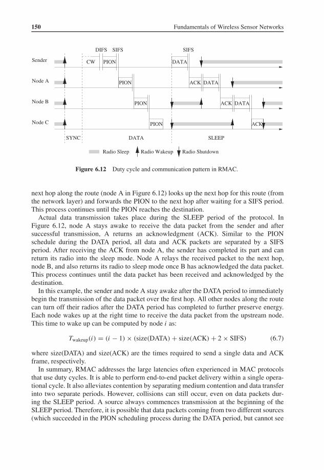
150 Fundamentals of Wireless Sensor Networks
Radio ShutdownRadio Sleep Radio Wakeup
Sender
Node A
Node B
Node C
DATA SLEEPSYNC
CW PION
PION
PION
PION
DIFS SIFS
DATA
ACK DATA
ACK
ACK
DATA
SIFS
Figure 6.12 Duty cycle and communication pattern in RMAC.
next hop along the route (node A in Figure 6.12) looks up the next hop for this route (fromthe network layer) and forwards the PION to the next hop after waiting for a SIFS period.This process continues until the PION reaches the destination.
Actual data transmission takes place during the SLEEP period of the protocol. InFigure 6.12, node A stays awake to receive the data packet from the sender and aftersuccessful transmission, A returns an acknowledgment (ACK). Similar to the PIONschedule during the DATA period, all data and ACK packets are separated by a SIFSperiod. After receiving the ACK from node A, the sender has completed its part and canreturn its radio into the sleep mode. Node A relays the received packet to the next hop,node B, and also returns its radio to sleep mode once B has acknowledged the data packet.This process continues until the data packet has been received and acknowledged by thedestination.
In this example, the sender and node A stay awake after the DATA period to immediatelybegin the transmission of the data packet over the first hop. All other nodes along the routecan turn off their radios after the DATA period has completed to further preserve energy.Each node wakes up at the right time to receive the data packet from the upstream node.This time to wake up can be computed by node i as:
Twakeup(i) = (i − 1) × (size(DATA) + size(ACK) + 2 × SIFS) (6.7)
where size(DATA) and size(ACK) are the times required to send a single data and ACKframe, respectively.
In summary, RMAC addresses the large latencies often experienced in MAC protocolsthat use duty cycles. It is able to perform end-to-end packet delivery within a single opera-tional cycle. It also alleviates contention by separating medium contention and data transferinto two separate periods. However, collisions can still occur, even on data packets dur-ing the SLEEP period. A source always commences transmission at the beginning of theSLEEP period. Therefore, it is possible that data packets coming from two different sources(which succeeded in the PION scheduling process during the DATA period, but cannot see

Medium Access Control 151
each other) may still collide. This problem has been addressed by a similar protocol calledDemand Wakeup (DW-MAC) (Sun et al. 2008a). In DW-MAC, the schedule is a one-to-onemapping between a DATA period and the following SLEEP period:
T Si = T D
i × Tsleep
Tdata(6.8)
where T Si is the start time of the scheduling frame (SCH) (the equivalent of the pioneer
frame in RMAC) measured from the start of the DATA period and T Di is the start time of the
data transmission in the SLEEP period (measured from the start of the SLEEP period). Tsleep
and Tdata are the durations of the SLEEP and DATA periods, respectively. This means thatdata packet transmissions do not necessarily coincide with the start of the SLEEP period,but instead depend on the contention window during the DATA period (the delay in datatransmission corresponds to the delay in the transmission of the SCH frame). This approach,compared to RMAC, reduces the risk of collisions during the SLEEP period.
6.5.6 Data-Gathering MAC
The Data-Gathering MAC (DMAC) (Lu et al. 2004) protocol exploits the fact that manywireless sensor networks rely on convergecast as communication pattern, that is, data fromsensor nodes are collected at a central node (the “sink”) in a data-gathering tree. The goalof DMAC is to deliver data along the data gathering tree with low latency and high energyefficiency.
In DMAC, the duty cycles of nodes along the multi-hop path to the sink are “staggered”;nodes wake up sequentially like a chain reaction. Figure 6.13 illustrates this concept, show-ing an example of a data-gathering tree and the staggered wakeup scheme. Nodes switchbetween sending, receiving, and sleep states. During the sending state, a node sends a packetto the next hop node on the route and awaits an acknowledgment (ACK). At the same time,the next hop node is in the receiving state, immediately followed by a sending state (unlessthe node is the destination of the packet) to forward the packet to the next hop. Betweenthese intervals of receiving and sending of packets, a node enters the sleep state, where itcan power down its radio to preserve energy.
The sending and receiving intervals are large enough for exactly one packet. Since thereare no queuing delays, a node at depth d in the tree can then deliver a packet to the sink within
RXSink
RX TX RX
RX
RX
RX
RX
TX
TX
TX
TX
TX
Sleep
Sleep
Sleep
RX
Figure 6.13 Data-gathering tree and convergecast communication in DMAC.

152 Fundamentals of Wireless Sensor Networks
d intervals. While limiting a node’s activity to brief intervals for sending and receivingreduces the contention, collisions still do occur. Particularly, nodes with the same depthin the tree will have synchronized schedules. In DMAC, if a sender does not receive anACK, it queues the packet until the next sending interval. After three failed retransmissions,the packet will be dropped. To reduce collisions, nodes do not transmit immediately at thebeginning of the sending slot, but instead have a backoff period (BP) plus a random timewithin a contention window.
When a node has multiple packets to send during a sending slot, it can increase its ownduty cycle and request other nodes along the route to the sink to do the same. This is imple-mented through a slot-by-slot renewal mechanism using a more data flag in the MAC header.A receiver checks for this flag and, if set, it returns an acknowledgment that has also the moredata flag set. It then stays awake to receive and forward one additional packet.
In summary, DMAC’s staggering technique achieves very low latency and nodes onlystay awake for brief receive and send intervals. Since many nodes in the data-gathering treeshare the same schedule, collisions will occur and DMAC only employs limited collisionavoidance methods. DMAC works best for networks in which transmission paths and ratesare well known and do not change over time.
6.5.7 Preamble Sampling and WiseMAC
WiseMAC (El-Hoiydi and Decotignie 2004) is a MAC protocol that is concerned with theenergy consumption of downlink communication in infrastructure-based sensor networks,that is, communication from a base station to the sensor nodes. To avoid energy consump-tion due to idle listening, WiseMAC relies on the preamble sampling technique (El-Hoiydi2002). In this technique, the base station transmits a preamble preceding the actual datatransmission to alert the receiving node (see left graph in Figure 6.14). All sensor nodessample the medium (listen to the channel) with a fixed period Tw, but with independent andconstant relative sampling schedule offsets. If the medium is busy, a sensor node continuesto listen until the medium becomes idle or a data frame is received. The preamble’s size isequal to the sampling period, which ensures that the receiver will be awake to receive thedata portion of the packet. This approach allows the energy-constrained sensor nodes to turnoff the radio when the channel is idle, without the risk of missing a packet. A disadvantageof this approach is that the size of the preamble affects the achievable throughput and that adevice must stay awake when a preamble is detected, even if it is not the intended receiver.
Preamble
PreambleBase Station
Sensor
Data
Time
Time
Base Station
Sensor
Time
TimeTw
Tp
Tw
Data
Figure 6.14 Preamble sampling.
Medium Access Control 153
WiseMAC improves upon this by adding a technique that lets a base station learn thesampling schedules of the destination, thereby allowing it to start the transmission ofthe preamble immediately before the receiver wakes up. This allows the base stationto reduce the size of the preamble as shown in the right graph of Figure 6.14. Further,since the data portion of the packet will start shortly after the receiver’s radio hasturned on, the awake time of the receiver is also shortened. A node’s schedule offsetis embedded into the acknowledgment (ACK) message, allowing the base station tolearn the sampling schedules. The duration of the preamble (Tp) is then determinedas the minimum of the destination’s sampling period (Tw) and a multiple of the clockdrift between the clock at the base station and on the receiver, which grows over time.Therefore, the preamble length depends on the traffic load: the preamble is shorter whentraffic is high (brief intervals between two consecutive communications) and larger underlow load.
In summary, WiseMAC implements energy-efficient wake/sleep schedules for sensornodes, while ensuring that all data transmissions from a base station to the sensors will bereceived (the receiver will be awake). However, the approach is inefficient for broadcastmessages since the preamble is likely to be very large, that is, it must span over thesampling points of all receiver devices. Finally, WiseMAC is also affected by the hiddenterminal problem, that is, a sender’s preamble can interfere with ongoing transmissionswhen the sender is not aware of this other transmission.
6.5.8 Receiver-Initiated MAC
Another contention-based solution is the Receiver-Initiated MAC (RI-MAC) protocol (Sunet al. 2008b), where a transmission is always initiated by the receiver of the data. Each nodewakes up periodically to check whether there is an incoming data packet. That is, immedi-ately after turning on its radio, a node checks if the medium is idle and, if so, broadcasts abeacon message, announcing that it is awake and ready to receive data. A node with pend-ing data to transmit stays awake and listens for a beacon from its intended receiver. Oncethis beacon has been received, the sender immediately transmits the data, which will beacknowledged by the receiver with another beacon (see left graph in Figure 6.15). That is,the beacon serves two purposes: it invites new data transmissions and it acknowledges pre-vious transmissions. If there is no incoming data packet for a certain amount of time afterthe beacon broadcast, the node goes back to sleep after waiting a certain time.
If there are multiple contending senders, a receiver uses its beacon frames to coordinatetransmissions. A field in the beacon, called the backoff window size (BW), specifies thewindow over which to select a backoff value. If the beacon does not contain a BW (the firstbeacon sent out after waking up does not contain a BW), senders immediately commencetransmission. Otherwise, each sender randomly selects a backoff value within BW and thereceiver increases the BW value in the next beacon when it detects a collision. The rightgraph in Figure 6.15 shows an example with two senders immediately transmitting datapackets after receiving the receiver’s beacon. The receiver notices the collision and sendsanother beacon, this time containing a BW. Should the transmission collide multiple timesand the receiver was not able to receive a packet for several beacon intervals, it simply goesto sleep without further attempts.

154 Fundamentals of Wireless Sensor Networks
Awake Interval
Sender
Receiver
Sender 1
Receiver
Sender 2
DATA
DATA
B B B
B B
B B
DATA
Collision
B B
B B
Backoff
Backoff
B
DATA
BB
B B
DATA
Data Reception
Data Transmission
DATA
DATA DATA
DATA
Figure 6.15 Data transmission from a single sender (left) and two contending senders (right).
In RI-MAC, the receiver is in control of when to receive data and it is responsible fordetecting collisions and recovering lost data. Since transmissions are triggered by beacons,the receiver will have very little overhead due to overhearing. On the other hand, sendersmust wait for the receiver’s beacon before they can transmit, potentially leading to largeoverhearing costs. Finally, when packets collide, the senders will retry until the receivergives up, potentially leading to more collisions in the network and to increased data deliverylatencies.
6.6 Hybrid MAC Protocols
Some MAC protocols do not easily fit into schedule-based or contention-based categories,but instead display characteristics of both categories, for example, they may attempt toreduce the number of collisions by relying on features present in periodic contention-freemedium access protocols, while taking advantage of the flexibility and low complexityof contention-based protocols. This section describes representative examples of hybridprotocols.
6.6.1 Zebra MAC
The Zebra MAC (Z-MAC) protocol (Rhee et al. 2005) uses frames and slots, similar toTDMA-based protocols, to provide contention-free access to the wireless medium. How-ever, Z-MAC also allows nodes to utilize slots they do not own using CSMA with prioritizedbackoff times. As a consequence, Z-MAC emulates a CSMA-based approach in low-trafficscenarios and a TDMA-based approach when traffic loads are high.
When a node starts up, it enters a setup phase to allow it to discover its neighbors andto obtain its slot in the TDMA frame. Every node periodically broadcasts a message con-taining a list of its neighbors. Through this process, a node learns about its 1-hop and 2-hopneighbors. This information is used as input to a distributed slot assignment protocol (Rheeet al. 2006), which provides each node with time slots, ensuring a schedule where no twonodes within a 2-hop neighborhood will be assigned the same slot. Further, Z-MAC allowsnodes to select the periodicity of their assigned slots, where different nodes can have dif-ferent periods, which are called time frames (TF). The advantage of this approach is thatit is not necessary to propagate a maximum slot number (MSN) to the entire network andthat the protocol can adapt slot allocations locally. Specifically, if node i is assigned slot si

Medium Access Control 155
and Fi represents the MSN within the node’s 2-hop neighborhood, then i’s TF is set to be2a , where a is a positive integer that satisfies 2a−1 ≤ Fi < 2a − 1. Node i then uses the si thslot in every 2a time frame.
Figure 6.16 shows an example with eight nodes, where the number indicates the assignedslot for each node and the number in parenthesis is Fi . The bottom part of the figure showsthe corresponding schedule for all nodes, where light-shaded slots are the ones used fortransmissions and dark-shaded slots are the empty slots that are not used by any 1-hopor 2-hop neighbors. If a global time frame is used, the chosen time frame size will be6 and nodes A and B will be allowed to use their slots only once every 6 slots (eventhough their frame sizes are 2 each). However, in Z-MAC, they can use frame size 4,which increases the concurrency in the channel usage and reduces message delays. Theresulting schedule shows that some slots (specifically slots 6 and 7) are not assigned toany node. In a global time frame, a frame size could have been chosen that reduces thenumber of empty slots. However, Z-MAC allows nodes to compete for these “extra” slotsusing CSMA.
After the schedule has been determined, every node forwards its frame size and slot num-ber to its 1-hop and 2-hop neighbors. Even though slots are owned by nodes, Z-MAC usesCSMA to determine who may transmit. However, slot owners are given preference by usinga random backoff value chosen from the range [0, To], whereas other nodes choose their
7
A
B
C
D
E
F
GH
0 (2)
1 (2)
2 (5)
0 (5)
1 (5)
3 (5)
4 (5)5 (5)
A
B
C
D
E
F
G
H
0 1 2 3 4 5 6
Figure 6.16 Selection of time frames and corresponding schedule for a Z-MAC network.

156 Fundamentals of Wireless Sensor Networks
backoff values from the range [To, Tno]. Z-MAC also uses explicit contention notification(ECN), where, based on its local estimate of the contention level (e.g., determined using thepacket loss rate or channel noise level), each node decides whether to send an ECN messageto a neighbor for which it has a message. This neighbor then broadcasts the ECN to its ownneighbors, which then enter a high contention level (HCL) mode. A node in the HCL modeonly transmits data in its own slots or slots belonging to its 1-hop neighbors, reducing thecontention between 2-hop neighbors. Nodes in HCL mode return to a low contention level(LCL) mode if they have not received any ECN messages for a certain amount of time.
In summary, Z-MAC adopts characteristics found in both TDMA and CSMA protocols,allowing it to quickly adapt to changing traffic conditions. Under light traffic loads, Z-MACbehaves more like CSMA, while under heavy traffic loads, contention for slots is reduced.Z-MAC requires an explicit setup phase, which consumes both time and energy. While ECNmessages can be used to reduce the contention locally, these messages add more traffic toan already busy network and take time to propagate, causing delays in the adaptation to amore TDMA-like behavior.
6.6.2 Mobility Adaptive Hybrid MAC
In many sensor networks, some or all nodes can be mobile, which can bear significant chal-lenges for the design of a MAC protocol. The Mobility Adaptive Hybrid MAC (MH-MAC)protocol (Raja and Su 2008) proposes a hybrid solution, where a schedule-based approachis used for static nodes and a contention-based approach is used for mobile nodes. Whileit is straightforward to determine a TDMA-style schedule for static nodes, this is not thecase for mobile nodes. Therefore, MH-MAC allows mobile nodes entering a neighborhoodto use a contention-based approach to avoid the delays often needed to be inserted into theschedule.
In MH-MAC, the slots of a frame belong to one of two categories: static slots or mobileslots. Each node uses a mobility estimation algorithm to determine its mobility and whichtype of slots the node should use. The mobility estimation is based on periodic hello mes-sages and received signal strength. The hello messages are always transmitted with the sametransmit power and the receiving nodes compare consecutive message signal strengths toestimate the relative position displacement between itself and each of its neighbors. A mobil-ity beacon interval is provided at the beginning of a frame to distribute mobility informationto neighbors.
Static slots use an approach similar to the LMAC approach described in Section 6.4.6, thatis, a static slot has two portions: a control section and a data section. The control section isused to indicate the slot assignment information in a neighborhood and all static nodes mustlisten to this part of the static slot. However, during the data section, only the transmitterand receiver stay awake and all other nodes can turn their radios off.
For mobile slots, nodes contend for the medium in a two-phase contention period. First, awakeup tone is sent during the first phase, and then the data is sent during the second phase.In order to reduce the effective contention, LMAC uses a priority ordering among mobilenodes based on node addresses.
Since the ratio between static and mobile nodes in a network can vary, MH-MAC providesa mechanism to dynamically adjust the ratio between static and mobile slots based on the

Medium Access Control 157
observed mobility. Each node estimates its own mobility and broadcasts this information inthe previously mentioned beacon time slot at the beginning of a frame. Using this mobilityinformation, each node calculates a mobility parameter for the network, which determinesthe ratio of static and mobile slots.
In summary, MH-MAC combines characteristics of the LMAC protocol for static nodesand features of contention-based protocols for mobile nodes. Therefore, mobile nodes canquickly join a network without long setup or adaptation delays. Compared to LMAC, MH-MAC allows nodes to own more than one slot in a frame, which increases bandwidth uti-lization and decreasing latencies.
6.7 Summary
The choice of a medium access protocol has a substantial impact on the performance andenergy-efficiency of a WSN. MAC protocols should also be designed to accommodatechanges in network topology and traffic characteristics. Further, latency, throughput, andfairness among competing nodes are also determined or affected by the characteristics of theMAC layer. This chapter discussed the major categories of medium access control protocolsand illustrated each category with several examples. A major distinction can be madebetween protocols that are based on transmission schedules (e.g., TDMA-style protocols)and protocols that do not use such schedules, but instead let nodes compete for the medium.The main advantage of schedule-based protocols is that communication can occur collision-free. However, such protocols can be resource-inefficient, may require well-synchronizednodes throughout the network, and are often difficult to adapt to changing topologies. Onthe other hand, contention-based solutions are more flexible in that they easily accommo-date changing network topologies. They typically also require less overhead. However,such protocols are not collision-free, so they must possess features that allow them torecover from collisions, and the network utilization may suffer when collisions occurfrequently.
Exercises
6.1 What is the main purpose of the MAC layer and why is this challenging in networkswith shared media?
6.2 What are the advantages and disadvantages of contention-free and contention-basedmedium access strategies? Can you think of scenarios where one would be preferableover the other?
6.3 The key idea behind CSMA/CD is that the sender detects collisions, allowing it toreact correspondingly. Why is this approach not practical in wireless networks?
6.4 What are “hidden terminals” and how do they affect the performance of wireless sensornetworks?
6.5 Consider the network topology in Figure 6.17, where circles indicate the communi-cation and interference range of each node, that is, each node can hear the immediateneighbors to the left and right. Assume that RTS/CTS is not being used.

158 Fundamentals of Wireless Sensor Networks
C D EBA F
Figure 6.17 Hidden-terminal problem (Exercise 6.5).
(a) Node B currently sends to node A and node C wants to send to node D. Is node Callowed to do so (i.e., can it do so without causing a collision) and will it decideto do so?
(b) Node C sends to node B and node E wants to send to node D. Is E allowed to doso and will it do so?
(c) Node A sends to node B and node D sends to node C. Which other nodes areallowed to send at the same time?
(d) Node A sends to node B and node E sends to node F. Which other nodes areallowed to send at the same time?
6.6 Describe the problems in using CSMA as a medium access control mechanism in aWSN.
6.7 In a CSMA/CA network, nodes use a random delay before accessing the medium. Whyis this being done?
6.8 Assume that the RTS and CTS frames were as long as the DATA and ACK frames.Would there be any advantage to using the RTS/CTS approach? Explain why or whynot.
6.9 How does MACAW extend MACA and what is the purpose of the additional controlmessages?
6.10 What are the specific features of the IEEE 802.11 PSM (Power Saving Mode) andwhat are the main difficulties of using it in wireless sensor networks?
6.11 Does the NAV field in IEEE 802.11 networks prevent the hidden terminal problem?
6.12 Explain why the IEEE 802.11 standard uses three different “interframe spaces”.
6.13 Consider the network topology in Figure 6.18, where the lines indicate which nodescan communicate and interfere with each other. Assume a TDMA protocol with aframe size of 5 slots and that each node can only be sender or receiver during any timeslot.
(a) Generate a schedule such that every node has an opportunity to communicate toall if its neighbors.
(b) For your schedule, how many slots in a frame could each node sleep to preserveenergy? What is your insight with respect to node density and energy preservation?

Medium Access Control 159
(c) Assume that node A sends a message to node E; how long (in number of timeslots) does it take for E to receive the message using your schedule? (Explain youranswer.)
BA
D
C
F
E
Figure 6.18 TDMA protocol (Exercise 6.13).
6.14 Why is the IEEE 802.15.4 standard preferable over the IEEE 802.11 standard for mostwireless sensor networks?
6.15 Describe how the design of the MAC protocol affects the energy efficiency of a sensornode.
6.16 This chapter described five requirements of MAC protocols for wireless sensor net-works: energy efficiency, scalability, adaptability, low latency, and reliability. Can youdescribe a concrete WSN application for each of these five requirements, where therequirement would be more important than the others?
6.17 The TRAMA protocol is an example of a contention-free MAC scheme. Answer thefollowing questions about TRAMA.
(a) What are the advantages and disadvantages of the TRAMA protocol (comparedto contention-based protocols)?
(b) What is the difference between transmission slots and signaling slots?(c) What is the purpose of the NP component?
6.18 What is the advantage of a receiver-initiated MAC scheme such as Y-MAC? What isthe main disadvantage of Y-MAC that makes it unsuitable for most low-power andlow-cost sensor nodes?
6.19 Demonstrate the concept of DESYNC using the example ring shown in Figure 6.19.The ring has 16 positions [0 . . . 15], with node A currently in position 0 (the firingposition), B in position 14, etc. Every unit of time, each node moves one positionclockwise along the ring. The table indicates the positions of the four nodes, includingthe new distance information that is learned at each firing. Assume that node A hasreceived D’s last firing, indicating a distance of 10 between nodes A and D. In thistable, at time 0, node A fires, allowing node B to learn its distance to A (i.e., 2). Attime 1, no node is in the firing position. At time 2, node B fires, allowing node C tolearn its distance to node B (i.e., 2). At the same time, node A now knows its distance

160 Fundamentals of Wireless Sensor Networks
to node B and its distance to node D. According to the description of the DESYNCalgorithm in this chapter, node A can now find the midpoint between nodes B and Dand jump to this new location (i.e., 6), which is indicated in the table at time 2. At time3, again each node moves ahead one position. Continue this table using the DESYNCalgorithm until time 19. Compare the average distance between neighboring nodes attime 19 with that of time 0.
DBC = 2
DAB = 2
7
01
2/6
1415
12131415
10111213
0123
01
fires Time DistancesB C D
A
C
D
B
A
Figure 6.19 DESYNC ring (Exercise 6.19).
6.20 Discuss the cluster head election policy in the LEACH protocol and explain howLEACH can consider the available energy on each node in this election process. Whatis the problem with this energy-aware election policy? Further, LEACH uses TDMAwithin a cluster; explain the advantages and disadvantages of this approach.
6.21 Why does LEACH use the direct sequence spread spectrum technique?
6.22 How does the Mobile LMAC protocol handle changes in network topology?
6.23 Discuss why overhearing is a problem in a wireless sensor network and explain howPAMAS addresses this problem.
6.24 Explain how the busy-tone scheme of PAMAS helps to avoid the hidden-terminalproblem.
6.25 How does the S-MAC protocol reduce the duty cycles of sensor nodes? How does theS-MAC protocol attempt to reduce collisions? How does it address the hidden-terminalproblem? Name at least three disadvantages of the S-MAC protocol.
6.26 Which shortcoming of S-MAC does T-MAC address? Explain briefly T-MAC’s abilityto adapt to traffic density.
6.27 What is the “early sleeping problem” and how does T-MAC address this problem?
6.28 Describe the concept behind PMAC’s approach to adapting a node’s sleep durationsto observed traffic.
6.29 The use of duty cycles allows nodes to alternate periods of activity and low-powersleep intervals. However, this often introduces large communication latencies.In Figure 6.20, node A wishes to send a packet to node F using the routeA–B–C–D–E–F. Assume that the interval between two dashed vertical lines is

Medium Access Control 161
one unit of time and that each transmission requires exactly one unit of time ofoverlapping periods of activity of two neighboring nodes. The first transmissionbetween A and its neighbor is already shown in the figure. Complete this graph todetermine the end-to-end latency experienced by the packet. Further, explain howRMAC reduces these end-to-end latencies and what would this latency be in anRMAC network? Finally, explain how the RMAC protocol reduces collisions.
Node F
Node A
Node B
Node C
Node D
Node E
Figure 6.20 RMAC duty cycle pattern (Exercise 6.29).
6.30 For what type of WSN applications would you use the DMAC protocol?
6.31 Explain the problem of “idle listing” and describe how preamble sampling addressesthis problem. How does WiseMAC improve upon “standard” preamble sampling?
6.32 What is the advantage of having the receiver (instead of the sender) in control overthe timing of transmissions (e.g., as in the RI-MAC protocol)? How does the RI-MACprotocol handle multiple contending senders?
6.33 Explain how the Z-MAC protocol allows nodes to determine their own local timeframes instead of using a single global time frame. What are the disadvantages ofZ-MAC?
ReferencesBharghavan, V., Demers, A., Shenker, S., and Zhang, L. (1994) MACAW: A medium access protocol for wireless
LANs. Proc. of the Conference on Communication Architectures, Protocols and Applications.CC1000 (2004) Single chip very low power RF transceiver. http://focus.ti.com/lit/ds/symlink/cc1000.pdf.CC2420 (2004) 2.4-GHz IEEE 802.15.4/ZigBee-ready RF transceiver datasheet. http://enaweb.eng.yale.edu/
drupal/system/files/CC2420 Data Sheet 1 4.pdf.Degesys, J., Rose, I., Patel, A., and Nagpal, R. (2007) DESYNC: Self-organizing desynchronization and TDMA
on wireless sensor networks. Proc. of the 6th International Conference on Information Processing in SensorNetworks (IPSN).
Du, S., Kumar, A., David, S., and Johnson, B. (2007) RMAC: A routing-enhanced duty-cycle MAC protocol forwireless sensor networks. Proc. of the 26th IEEE International Conference on Computer Communications(INFOCOM).
El-Hoiydi, A. (2002) Spatial TDMA and CSMA with preamble sampling for low power ad hoc wireless sensornetworks. Proc. of the 7th IEEE Symposium on Computers and Communications .
El-Hoiydi, A., and Decotignie, J.D. (2004) WiseMAC: An ultra low power MAC protocol for the downlink ofinfrastructure wireless sensor networks. Proc. of the 9th IEEE Symposium on Computers and Communication .
Gutierrez, J.A., Naeve, M., Callaway, E., Bourgeois, M., Mitter, V., and Heile, B. (2001) IEEE 802.15.4: A devel-oping standard for low-power low-cost wireless personal area networks. IEEE Network 15 (5), 12–19.

162 Fundamentals of Wireless Sensor Networks
Heinzelman, W.B., Chandrakasan, A.P., and Balakrishnan, H. (2002) An application specific protocol architecturefor wireless microsensor networks. IEEE Transactions on Wireless Communications .
Karn, P. (1990) A new channel access method for packet radio. Proc. of the ARRL 9th Computer NetworkingConference.
Kim, Y., Shin, H., and Cha, H. (2008) YMAC: An energy-efficient multi-channel MAC protocol for dense wirelesssensor networks. Proc. of the International Conference on Information Processing in Sensor Networks (IPSN).
Kuo, F.F. (1995) The ALOHA system. ACM SIGCOMM Computer Communication Review 25 (1), 41–44.Lu, G., Krishnamachari, B., and Raghavendra, C.S. (2004) An adaptive energy-efficient and low-latency MAC for
data gathering in wireless sensor networks. Proc. of the 18th International Parallel and Distributed ProcessingSymposium .
Mank, S., Karnapke, R., and Nolte, J. (2007) An adaptive TDMA based MAC protocol for mobile wireless sensornetworks. Proc. of the International Conference on Sensor Technologies and Applications (SENSORCOMM).
MC13202 (2008) 2.4-GHz low power transceiver for the IEEE 802.15.4 standard. www.freescale.com/files/rf if/doc/data sheet/MC13202.pdf.
Raja, A., and Su, X. (2008) A mobility adaptive hybrid protocol for wireless sensor networks. Proc. of the Con-sumer Communications and Networking Conference.
Rajendran, V., Obraczka, K., and Garcia Luna Aceves, J.J. (2003) Energy efficient, collision free medium accesscontrol for wireless sensor networks. Proc. of the 1st International Conference on Embedded Networked SensorSystems (SenSys).
Rhee, I., Warrier, A., Aia, M., and Min, J. (2005) ZMAC: A hybrid MAC for wireless sensor networks. Proc. ofthe 3rd ACM Conference on Embedded Networked Sensor Systems (SenSys).
Rhee, I., Warrier, A., Min, J., and Xu, L. (2006) DRAND: Distributed randomized TDMA scheduling for wire-less ad hoc networks. Proc. of the 7th ACM International Symposium on Mobile Ad Hoc Networking andComputing (MobiHoc).
Singh, S., and Raghavendra, C. (1998) PAMAS: Power aware multi-access protocol with signaling for ad hocnetworks. SIGCOMM Computer Communications Review 28 (3), 5–26.
Sun Y., Du, S., Gurewitz, O., and Johnson, D.B. (2008a) DWMAC: Low latency, energy efficient demand wakeupMAC protocol for wireless sensor networks. Proc. of the 9th International Symposium on Mobile Ad HocNetworking and Computing (MobiHoc).
Sun, Y., Gurewitz, O., and Johnson, D.B. (2008b) RIMAC: A receiver initiated asynchronous duty cycle MACprotocol for dynamic traffic loads in wireless sensor networks. Proc. of the 6th ACM Conference on EmbeddedNetworked Sensor Systems (SenSys).
Talucci, F., Gerla, M., and Fratta, L. (1997) MACABI (MACA By Invitation): A receiver oriented access protocolfor wireless multi-hop networks. Proc. of the 8th IEEE International Symposium on Personal, Indoor andMobile Radio Communications .
Van Dam, T., and Langendoen, K. (2003) An adaptive energy-efficient MAC protocol for wireless sensor networks.Proc. of the 1st ACM Conference on Embedded Networked Sensor Systems (SenSys).
Van Hoesel, L., and Havinga, P. (2004) A lightweight medium access protocol (LMAC) for wireless sensornetworks: Reducing preamble transmissions and transceiver state switches. Proc. of the 1st International Con-ference on Networked Sensing Systems (INSS).
Ye, W., Heidemann, J., and Estrin, D. (2002) An energy-efficient MAC protocol for wireless sensor networks. Proc.of the 21st Annual Joint Conference of the IEEE Computer and Communications Societies (INFOCOM).
Ye, W., Heidemann, J., and Estrin, D. (2004) Medium access control with coordinated active sleeping for wirelesssensor networks. IEEE/ACM Transactions on Networking 12 (3), 493–506.
Zheng, T., Radhakrishnan, S., and Sarangan, V. (2005) PMAC: An adaptive energy-efficient MAC protocol forwireless sensor networks. Proc. of the 19th IEEE International Parallel and Distributed Processing Sympo-sium (IPDPS).

7Network LayerData collected by sensor nodes in a WSN is typically propagated toward a base station(gateway) that links the WSN with other networks where the data can be visualized, ana-lyzed, and acted upon. In small sensor networks where sensor nodes and a gateway are inclose proximity, direct (single-hop) communication between all sensor nodes and the gate-way may be feasible. However, most WSN applications require large numbers of sensornodes that cover large areas, necessitating an indirect (multi-hop) communication approach.That is, sensor nodes must not only generate and disseminate their own information, but alsoserve as relays or forwarding nodes for other sensor nodes. The process of establishing pathsfrom a source to a sink (e.g., a gateway device) across one or more relays is called routingand is a key responsibility of the network layer of the communication protocol stack. Whenthe nodes of a WSN are deployed in a deterministic manner (i.e., they are placed at certainpredetermined locations), communication between them and the gateway can occur usingpredetermined routes. However, when the nodes are deployed in a randomized fashion (i.e.,they are scattered into an environment randomly), the resulting topologies are nonuniformand unpredictable. In this case, it is essential for these nodes to self-organize, that is, theymust cooperate to determine their positions, identify their neighbors, and discover paths tothe gateway device. This chapter introduces the main categories of routing protocols anddata dissemination strategies and discusses state-of-the-art solutions for each category.
7.1 Overview
The key responsibility of the network layer is to find paths from data sources to sink devices(e.g., gateways). In the single-hop routing model (left graph in Figure 7.1), all sensor nodesare able to communicate directly with the sink device. This direct communication model isthe simplest approach, where all data travels a single hop to reach the destination. However,in practical settings, this single-hop approach is unrealistic and a multi-hop communica-tion model (right graph in Figure 7.1) must be used. In this case, the critical task of thenetwork layer of all sensor nodes is to identify a path from the sensor to the sink across mul-tiple other sensor nodes acting as relays. This design of a routing protocol is challengingdue to the unique characteristics of WSNs, including resource scarcity or the unreliabil-ity of the wireless medium. For example, the limited processing, storage, bandwidth, andenergy capacities require routing solutions that are lightweight, while the frequent dynamicchanges in a WSN (e.g., topology changes due to node failures) require routing solutions
Fundamentals of Wireless Sensor Networks: Theory and Practice Waltenegus Dargie and Christian Poellabauer 2010 John Wiley & Sons, Ltd

164 Fundamentals of Wireless Sensor Networks
SINK
SENSOR
SENSOR
SINK
Figure 7.1 Single-hop routing model (left) versus multi-hop routing model (right).
that are adaptive and flexible. Further, unlike traditional routing protocols for wired net-works, protocols for sensor networks may not be able to rely on global addressing schemes(e.g., IP addresses on the Internet).
There are various ways to classify routing protocols. Figure 7.2 presents three differentclassifications based on the network structure or organization, the route discovery process,and the protocol operation (Al-Karaki and Kamal 2004). With respect to network orga-nization, most routing protocols fit into one of three classes. Flat-based routing protocolsconsider all nodes of equal functionality or role. In contrast, in hierarchical-based routingprotocols, different nodes may assume different roles in the routing process, that is, somenodes may forward data on behalf of others, while other nodes only generate and propagatetheir own sensor data. Location-based routing protocols rely on the location informationfrom nodes to make routing decisions. Routing protocols are responsible for identifying ordiscovering routes from a source or sender to the intended receiver. This route discoveryprocess can also be used to distinguish between different types of routing protocols. Reac-tive protocols discover routes on-demand , that is, whenever a source wants to send datato a receiver and does not already have a route established. While reactive route discovery
Coherent-Based
Routing Protocol
Network Organization
Flat-Based
Route Discovery
Reactive Proactive Hybrid
Location-Based
Hierarchical-Based
Protocol Operation
Negotiation-Based
Multi-Path-Based
Query-Based
QoS-Based
Figure 7.2 Categories of routing protocols.
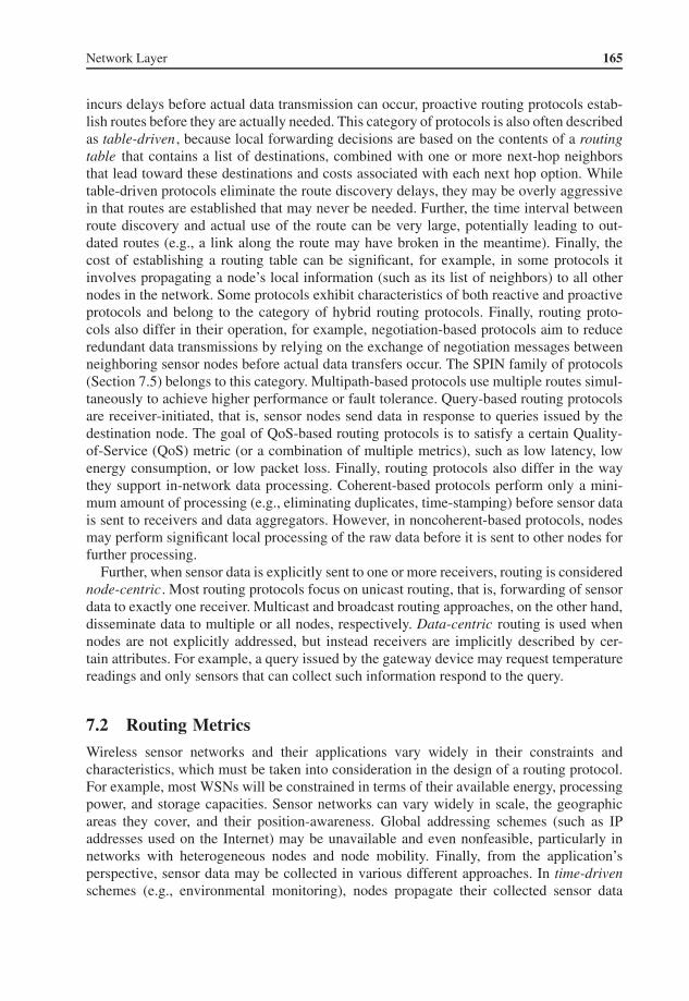
Network Layer 165
incurs delays before actual data transmission can occur, proactive routing protocols estab-lish routes before they are actually needed. This category of protocols is also often describedas table-driven, because local forwarding decisions are based on the contents of a routingtable that contains a list of destinations, combined with one or more next-hop neighborsthat lead toward these destinations and costs associated with each next hop option. Whiletable-driven protocols eliminate the route discovery delays, they may be overly aggressivein that routes are established that may never be needed. Further, the time interval betweenroute discovery and actual use of the route can be very large, potentially leading to out-dated routes (e.g., a link along the route may have broken in the meantime). Finally, thecost of establishing a routing table can be significant, for example, in some protocols itinvolves propagating a node’s local information (such as its list of neighbors) to all othernodes in the network. Some protocols exhibit characteristics of both reactive and proactiveprotocols and belong to the category of hybrid routing protocols. Finally, routing proto-cols also differ in their operation, for example, negotiation-based protocols aim to reduceredundant data transmissions by relying on the exchange of negotiation messages betweenneighboring sensor nodes before actual data transfers occur. The SPIN family of protocols(Section 7.5) belongs to this category. Multipath-based protocols use multiple routes simul-taneously to achieve higher performance or fault tolerance. Query-based routing protocolsare receiver-initiated, that is, sensor nodes send data in response to queries issued by thedestination node. The goal of QoS-based routing protocols is to satisfy a certain Quality-of-Service (QoS) metric (or a combination of multiple metrics), such as low latency, lowenergy consumption, or low packet loss. Finally, routing protocols also differ in the waythey support in-network data processing. Coherent-based protocols perform only a mini-mum amount of processing (e.g., eliminating duplicates, time-stamping) before sensor datais sent to receivers and data aggregators. However, in noncoherent-based protocols, nodesmay perform significant local processing of the raw data before it is sent to other nodes forfurther processing.
Further, when sensor data is explicitly sent to one or more receivers, routing is considerednode-centric. Most routing protocols focus on unicast routing, that is, forwarding of sensordata to exactly one receiver. Multicast and broadcast routing approaches, on the other hand,disseminate data to multiple or all nodes, respectively. Data-centric routing is used whennodes are not explicitly addressed, but instead receivers are implicitly described by cer-tain attributes. For example, a query issued by the gateway device may request temperaturereadings and only sensors that can collect such information respond to the query.
7.2 Routing Metrics
Wireless sensor networks and their applications vary widely in their constraints andcharacteristics, which must be taken into consideration in the design of a routing protocol.For example, most WSNs will be constrained in terms of their available energy, processingpower, and storage capacities. Sensor networks can vary widely in scale, the geographicareas they cover, and their position-awareness. Global addressing schemes (such as IPaddresses used on the Internet) may be unavailable and even nonfeasible, particularly innetworks with heterogeneous nodes and node mobility. Finally, from the application’sperspective, sensor data may be collected in various different approaches. In time-drivenschemes (e.g., environmental monitoring), nodes propagate their collected sensor data

166 Fundamentals of Wireless Sensor Networks
periodically to a sink or gateway device. In event-driven schemes (e.g., wildfire detection),nodes only report their collected information when events of interest occur. Finally, inquery-driven schemes, it is the responsibility of the sink to request data from sensors whenneeded. Regardless of the scheme used in the network, the design of a routing protocol isdriven by the resources available in the network and the needs of the applications. Towardthis end, routing metrics are used to express a variety of objectives of a routing protocol withrespect to the consumption of these resources or the performance an application perceives.This section provides a brief overview of commonly used routing metrics in WSNs.
7.2.1 Commonly Used Metrics
7.2.1.1 Minimum Hop
The most common metric used in routing protocols is minimum hop (or shortest hop), thatis, the routing protocol attempts to find the path from the sender to the destination thatrequires the smallest number of relay nodes (hops). In this simple technique, every link hasthe same cost and a minimum-hop routing protocol selects the path that minimizes the totalcost of data propagation from source to destination. The basic idea behind this metric is thatusing the shortest path will result in low end-to-end delays and low resource consumptions,because the smallest possible number of forwarding nodes will be involved. However, sincethe minimum-hop approach does not consider the actual resource availability on each node,the resulting route is probably nonoptimal in terms of delay, energy, and congestion avoid-ance. Nevertheless, the minimum-hop metric is being used in many routing protocols dueto its simplicity and its isotonicity, that is, its ability to ensure that the order of weights oftwo paths is preserved even when they are appended or prefixed by a common third path.
7.2.1.2 Energy
Undoubtedly the most crucial aspect of routing in WSNs is energy efficiency. However,there is not one unique energy metric that can be applied to the routing problem; instead,there are various different interpretations of energy efficiency, including (Singh et al. 1998):
1. Minimum energy consumed per packet: This is the most natural concept of energy effi-ciency, that is, the goal is to minimize the total amount of energy expended for thepropagation of a single packet from the source to the destination. The total energy is thenthe sum of the energy consumed by each node along a route for receiving and transmit-ting the packet. Figure 7.3 shows an example of a small sensor network, where a sourcenode wishes to transmit a packet to a destination node using a route that minimizes thepacket’s energy overheads. The number on each link indicates the cost of propagatingthe packet over this link. As a consequence, the packet will travel via nodes A–D–G(with a total cost of 5). Note that this is different from the minimum-hop route (B–G).
2. Maximum time to network partition: A network partitions into several smaller sub-networks when the last node that links two parts of the network expires or fails. As aconsequence, a subnetwork may not be reachable, rendering the sensor nodes within thesubnetwork useless. Therefore, the challenge is to reduce the energy consumption onnodes that are crucial to maintaining a network where every sensor node can be reached

Network Layer 167
(2)
1
2
1D
(3)
(1) (2)
(2) (1)
3
4
(1)
(5)
(2)
A
C
B
E
G
H
1
21
1
2
2
3
2
1
22
F
I
J
Source
Destination
Figure 7.3 Comparison of routing choices using different energy metrics.
via at least one route. For example, a minimal set of nodes, whose removal will cause anetwork to partition, can be found using the max-flow–min-cut theorem. Once a routingprotocol has identified these critical nodes, it can attempt to balance the traffic load suchthat premature expiration of these nodes is prevented. In Figure 7.3, node D is such anode, for example, if node D’s battery becomes depleted, nodes F, I, and J would not bereachable from any other node in the network.
3. Minimum variance in node power levels: In this scenario, all nodes within the networkare considered equally important and the challenge is to distribute the energy consump-tion across all nodes in the network as equally as possible. The goal of such an approachcould be to maximize the lifetime of the entire network, for example, instead of somenodes expiring sooner than others and thereby continuously decreasing the network size,one could aim at keeping as many nodes alive as long as possible. In the ideal (but prac-tically impossible) case, all nodes would expire at exactly the same time.
4. Maximum (average) energy capacity: In this approach, the focus is less on the energycost of packet propagation, but instead on the energy capacity (i.e., the current batterycharge level) of the nodes. A routing protocol that uses this metric would then favor routesthat have the largest total energy capacity from source to destination. In Figure 7.3, thenumbers in parentheses below the nodes indicate the nodes’ remaining energy capacity.In this example, a routing protocol could select path C–E–G, which has the largest totalcapacity (i.e., 8). A routing protocol that uses this metric must be carefully designed toavoid the pitfall of choosing unnecessarily long routes in order to maximize the totalenergy capacity. A variation of this metric is to maximize the average energy capacity,which can avoid this problem.
5. Maximum minimum energy capacity: Finally, instead of maximizing the energy capaci-ties of the entire path, the primary routing goal could be to select the path with the largestminimum energy capacity. This technique also favors routes with larger energy reserves,but also protects low-capacity nodes from premature expiration. In Figure 7.3, a protocolusing this metric would choose B–G, since the minimum capacity along this route is 2,which is larger than the minimum capacities of all other possible routes.
These different formulations of energy awareness lead to very different protocol imple-mentations that differ in their results (i.e., the selected routes) and their overheads. For

168 Fundamentals of Wireless Sensor Networks
example, to determine the minimum energy consumed per packet, the cost for receivingand transmitting a packet may be based on a cost function with the packet size as input. Onthe other hand, energy capacities change over time and therefore a routing protocol using acapacity-based metric must obtain these capacities from other nodes from time to time.
7.2.1.3 Quality-of-Service
The term Quality-of-Service (QoS) refers to defined measures of performance in networks,including end-to-end latency (or delay) and throughput, but also jitter (variation in latency)and packet loss (or error rate). The choice of a QoS metric depends on the type ofapplication. Sensor networks performing target detection and tracking will require lowend-to-end transmission delays for their time-sensitive sensor data, while data-intensivenetworks (e.g., multimedia sensor networks) may require high throughput. The ExpectedTransmission Time (ETT) is a common metric to express latency and is defined as(Draves et al. 2004):
ETT = ETT × S
B(7.1)
where S is the average size of a packet and B is a link’s bandwidth. It expresses the expectedtime necessary to successfully transmit a packet at the MAC layer. To capture packet loss asa routing metric, the Expected Transmission Count (ETX) can be used, which is defined asthe number of transmissions necessary to successfully deliver a packet over a wireless link(Couto et al. 2003). Very often multiple QoS metrics (e.g., end-to-end latency and packetloss rate) are combined, for example, the bandwidth-delay product refers to the product ofa link’s bandwidth and its end-to-end delay. Which metrics are chosen affects the designof the network at different levels, including the network (routing) and MAC layers. MostWSNs must strike a balance between satisfying the application-specific QoS requirementsand the goal of energy efficiency in the network as whole.
7.2.1.4 Robustness
Many sensor applications may wish to use routes that stay stable and reliable for long periodsof time. Toward this end, a node can measure or estimate the link quality to each of itsneighbors and then select a next hop neighbor that increases the probability of a successfultransmission. However, this metric is rarely used alone. A routing protocol could identifyseveral minimum-hop paths and then select the one with the highest total or average linkquality along these paths. In networks with mobile nodes, a routing protocol could also usethe link stability metric, which measures how likely it is that a link will be available inthe future. These metrics can be used to bias route selection toward more robust paths andstationary nodes.
7.3 Flooding and Gossiping
An old and simple strategy to disseminate information into a network or to reach a nodeat an unknown location is to flood the entire network. A sender node broadcasts packetsto its immediate neighbors, which will repeat this process by rebroadcasting the packets totheir own neighbors until all nodes have received the packets or the packets have traveled

Network Layer 169
for a maximum number of hops. With flooding, if there exists a path to the destination (andassuming lossless communication), the destination is guaranteed to receive the data. Themain advantage of flooding is its simplicity, while its main disadvantage is that it causesheavy traffic. Therefore, measures must be taken to ensure that packets do not travel throughthe network indefinitely. For example, maximum-hop counts are used to limit the numberof times a packet is forwarded. It should be set large enough so that every intended receivercan be reached, but also small enough to ensure that packets do not travel too long in thenetwork. Further, sequence numbers in packets (combined with the address of the source)can be used to uniquely identify a packet. When a node receives a packet that it has alreadyforwarded (i.e., with the same destination–source pair and the same sequence number),it simply discards this duplicate. However, even with these mechanisms, flooding faces anumber of additional challenges (Heinzelman et al. 1999):
1. Implosion: A node receiving a packet relays this packet to all its neighbors using broad-casting, regardless of whether these neighbors have already received this packet fromother neighbors. This leads to resource waste due to unnecessary transmit-and-receiveoperations. The left graph in Figure 7.4 illustrates this problem. Node A broadcasts packetP1 to both of its neighbors, B and C. B forwards this packet to its own neighbor D and,finally, C also forwards this packet to node D. Even if D discards the duplicate packet,energy has been wasted on the transmission of the packet from C to D.
2. Overlap: Sensors are often used to monitor overlapping geographic areas, as illustratedin the right graph in Figure 7.4. Here, sensors A and B share the region marked as Y.Therefore, these sensors gather overlapping data and both forward their collected infor-mation to their neighbor C. Similar to the implosion problem, this also leads to resourcewaste since the same information is sent twice to the same receiver. Unlike the implo-sion problem, the overlap problem is more difficult to address, because a solution to thisproblem must not only consider the topology of the sensor network, but also the mappingof the collected sensor information to sensor nodes.
3. Resource Blindness: The simplicity of the protocol also means that flooding is incog-nizant of the resource constraints of individual nodes. As a consequence, flooding is notable to adapt its behavior based on the amount of energy available to a specific node.
A variation of flooding is gossiping (Hedetniemi et al. 1988), where a node does not nec-essarily broadcast data. Instead, it uses a probabilistic approach, where it decides to forwardthe data to its own neighbors with a probability p and to discard the data with a probability
A
B
D
P1 P1
P1 P1
A
C
XY
D(X,Y) D(Z,Y)
C B
Z
Figure 7.4 The implosion problem (left) and the overlap problem (right).

170 Fundamentals of Wireless Sensor Networks
1 − p. It therefore can reduce the amount of traffic and achieve energy conservation byrandomization. However, this only addresses the implosion problem of flooding, not theoverlapping and resource blindness problems. With gossiping, it is also possible that deliv-ery of sensor data fails when, for example, a node’s only neighbor decides not to forward thedata to this node. If a high probability for forwarding is chosen, the consequence is that themessage volume will be high (a probability of 1 corresponds to classic flooding), therebylimiting the benefits of gossiping. On the other hand, if the probability is low, the overheadcan be significantly smaller, but the probability of unsuccessful data delivery will increase.
7.4 Data-Centric Routing
In most sensor networks, the sensor nodes themselves are less important than the informationthey generate. Therefore, in data-centric routing techniques, the focus is on the retrievaland dissemination of information of a particular type or described by certain attributes, asopposed to the data collection from particular sensors. This section provides an overviewof data-centric routing and dissemination protocols in flat-based networks, where all nodesplay the same role concerning routing and all nodes collaborate to perform the routing task(i.e., no topology management is necessary).
7.4.1 Sensor Protocols for Information via Negotiation
Sensor Protocols for Information via Negotiation (SPIN) (Kulik et al. 2002) is a family ofnegotiation-based, data-centric, and time-driven flooding protocols. However, compared toclassic flooding, SPIN nodes rely on two key techniques to overcome the deficiencies offlooding. To address the problems of implosion and overlap, SPIN nodes negotiate withtheir neighbors before they transmit data, allowing them to avoid unnecessary communi-cations. To address the problem of resource blindness, each SPIN node uses a resourcemanager to keep track of actual resource consumption, allowing them to adapt routing andcommunication behavior based on resource availability.
SPIN uses meta-data to succinctly and completely describe the data collected by sensornodes. To ensure that the meta-data is useful for SPIN, a key requirement is that if x describesthe meta-data for some sensor data X, the size of x (in bytes) must be less than the size of X.Further, two identical pieces of sensor data should have the same meta-data representation.Similarly, if two pieces of sensor data differ, their meta-data representations should differtoo. The actual translation of sensor data to meta-data is application-specific and SPIN relieson each application to interpret and synthesize its own meta-data. For example, a camerasensor may use (x, y, φ) as meta-data, where (x, y) is a geographic coordinate and φ is anorientation.
7.4.1.1 SPIN-PP
The first member of the SPIN family, SPIN-PP, is optimized for networks using point-to-point transmission media, where two nodes can communicate exclusively with each otherwithout interference from other nodes. In SPIN-PP, data is flooded in three steps via a 3-wayhandshake protocol (Figure 7.5). First, when new data arrives, a node advertises this event

Network Layer 171
DC
B
A
E
DC
A
B
A
E
DC
B EADV
ADV
ADV
ADV REQ
REQ
DATA
DATA
(c)(a) (b)
Figure 7.5 The SPIN-PP protocol: (a) advertisement phase, (b) request phase, and (c) data trans-mission.
using an advertisement message (ADV) to its neighbors via the data’s meta-data. Uponreceiving an advertisement, a node checks whether it has already received the describedsensor data. If not, the node responds with a request for data (REQ) message, indicating itsdesire to receive the advertised data. Finally, the sender node responds to the REQ messagewith a DATA message, containing the advertised data.
As shown in Figure 7.5(b), only nodes that do not yet possess a copy of the advertiseddata respond to an ADV message. Further, upon receiving the DATA message from A, nodesB and D can aggregate this data with their own data and advertise the aggregate to theirneighbors. A key strength of this protocol is its simplicity and nodes only need to knowtheir single-hop neighbors to run this protocol. While this protocol has been designed forlossless environments with symmetric communication links, nodes could compensate forlost ADV messages by periodically readvertising their data and for lost REQ and DATAmessages by rerequesting data of interest if such data does not arrive within certain timeoutintervals. As an alternative, the protocol could be modified to use explicit acknowledgments.For example, REQ messages could contain explicit lists of data that a node wants or doesnot want to receive. Based on the list, a node can identify if previous advertisements weresuccessfully received by the neighbor.
7.4.1.2 SPIN-EC
A variation of this protocol, called SPIN-EC, adds a simple heuristic to add energy conser-vation to the SPIN-PP protocol. As long as all nodes have sufficient energy, they participatein the three-way handshake of the SPIN-PP protocol. However, once the energy of a nodeapproaches a specific low-energy threshold , it becomes more selective in its participation inthe protocol. That is, a node should only participate in the three-way handshake if it believesthat it can complete all stages of the protocol without falling below the energy threshold.Therefore, a node replies to an advertisement only if it has sufficient energy to transmit therequest and receive the requested data. Similarly, a node initiates the three-way handshakewith its neighbors only if it believes that it can complete the protocol even if all neighborsrequest a copy of the data.
7.4.1.3 SPIN-BC
While the SPIN-PP and SPIN-EC protocols assume point-to-point communicationnetworks, the SPIN-BC protocol improves upon these protocols by exploiting the

172 Fundamentals of Wireless Sensor Networks
characteristics of broadcast transmission. In broadcast transmission, every message sentby a sender will be received by all nodes within the sender’s radio range. SPIN-BC usescheap, one-to-many communications and nodes can coordinate their resource-conservingefforts more effectively because they are able to overhear all transactions within theirradio ranges.
The SPIN-BC uses a three-way handshake consisting of ADV, REQ, and DATA messages,but with three central differences compared to the approaches taken by SPIN-PP:
1. All messages are directed to the broadcast message, that is, all nodes within a sender’stransmission range will receive a copy of the message.
2. Upon receiving an ADV message, a node checks whether it wishes to receive a copy ofthe advertised data, and if so, sets a random timer, uniformly chosen from a predeter-mined interval. Only after the timer expires, the node issues the REQ message, again tothe broadcast address (specifying the identity of the sender of the ADV message in themessage header). When a node overhears the REQ message before its own timer expires,the node cancels its timer and does not send its own REQ message.
3. The advertiser transmits the advertised data to the broadcast address only once, that is, itwill ignore duplicate REQ messages for the same data.
The random timer is necessary to avoid collisions of REQ messages from different neighborsand to allow nodes to avoid REQ transmissions when another node has already transmittedan REQ. The consequence of this approach is that the number of transmissions can be sig-nificantly reduced, for example, for each transmission, a node needs only to transmit a singleADV message and a single copy of the DATA message.
7.4.1.4 SPIN-RL
The final variant of the SPIN protocol is SPIN-RL, a reliable version of SPIN-BC, addressingpacket loss and asymmetric communications. First, each node keeps track of overheard REQmessages and if it does not receive a corresponding DATA message within a certain timeoutinterval, it assumes that either the REQ message or the DATA message did not arrive. In thiscase, the node rerequests the data by broadcasting an REQ message, specifying the identityof a randomly selected node among the nodes that previously advertised this data in themessage header. In addition, SPIN-RL limits the frequency with which DATA messages aresent out. That is, once a node sends a DATA message, it will wait a predetermined timebefore responding to any other requests for the same data.
7.4.2 Directed Diffusion
Directed diffusion (Intanagonwiwat et al. 2000) is another data-centric data disseminationprotocol that is also application-aware in that data generated by sensor nodes is namedby attribute-value pairs. The main idea of directed diffusion is that nodes request data bysending interests for named data. This interest dissemination sets up gradients within thenetwork that are used to direct sensor data toward the recipient, and intermediate nodesalong the data paths can combine data from different sources to eliminate redundancy andreduce the number of transmissions.

Network Layer 173
Directed diffusion does not rely on globally valid node identifiers, but instead usesattribute-value pairs to describe a sensing task and to steer the routing process. For example,a description for a simple vehicle-tracking application could be:
type = vehicle // detect vehicle location
interval = 20 ms // send data every 20 ms
duration = 10 s // perform task for 10 s
rect = [-100,-100,200,200] // from sensors within rectangle
That is, a task description expresses a node’s desire (or interest) to receive data matchingthe provided attributes. The data sent in response to such interests is also named in the samemanner, that is, using attribute-value pairs.
Once an application has been described using this naming approach, the interest must bediffused through the sensor network. This process is shown in Figure 7.6. A sink node peri-odically broadcasts an interest message to its neighbors, which continue to broadcast themessage throughout the network (Figure 7.6(a)). Each node establishes a gradient towardthe sink node, where a gradient is a reply link toward the neighbor from which the interestwas received. As a consequence, using interests and gradients, paths between event sourcesand sinks can be established (Figure 7.6(b)). Once a source begins to transmit data, it canuse multiple paths for transmission toward the sink. The sink can then reinforce one partic-ular neighbor based on some data-driven local rule. For example, a sink could reinforce aneighbor from which the sink has received a previously unseen event. Toward this end, thesink resends the original interest message to the neighbor, which in turn reinforces one ormore of its neighbors based on its own local rule (Figure 7.6(c)).
Directed diffusion differs from SPIN in that queries (interests) are issued on demand bythe sinks and not advertised by the sources as in SPIN. Based on the process of establish-ing gradients, all communication is neighbor-to-neighbor, removing the need for address-ing schemes and allowing each node to perform aggregation and caching of sensor data,both of which can contribute to reduced energy consumption. Finally, directed diffusion
Source
Sink
Source
Sink
Interests
Source
Sink
(c)
Gradients
(a) (b)
Figure 7.6 Directed diffusion: (a) interest propagation, (b) initial gradients set up, and (c) datadelivery.

174 Fundamentals of Wireless Sensor Networks
is a query-based protocol, which may not be a good choice for certain sensor networkapplications, particularly where continuous data transfers are required (e.g., environmentalmonitoring applications).
7.4.3 Rumor Routing
While the classic flooding approach can be described as event flooding (i.e., a source prop-agates its sensor data via an event throughout the network), query flooding describes theprocess used to propagate queries to all nodes in the network when no localization informa-tion is available to steer the query toward the appropriate sensors. Rumor routing (Braginskyand Estrin 2002) is a variation of directed diffusion that attempts to combine the character-istics of both techniques.
In rumor routing, each node maintains a list of its neighbors and an event table that con-tains forwarding information to all known events. Once a node witnesses an event (i.e., aphenomenon in the physical world), the event is added to this table (including a distance ofzero) and an agent is generated with a certain probability (i.e., not all events may result inan agent generation). This agent is a long-lived packet that travels the network to propagateinformation about this event and other events encountered along its route to remote nodes.Once an agent arrives at a node, the node can use the agent’s content to update its own table.For example, in Figure 7.7(a), the table for node A pointing toward events E1 and E2 isshown, before the arrival of an agent originating at node E. When the agent arrives at nodeA (via node G), A sees that E1 can be reached via neighbor G using a shorter route than cur-rently stored in its table. It therefore updates its table with the newly obtained informationfrom E’s agent (Figure 7.7(b)).
When a node wants to issue a query targeted at a specific event, it first checks whether ithas a route toward the target event. If so, it forwards the query to the neighbor indicated bythe event’s table entry. If there is no route, a random neighbor is selected and the query ispassed to this neighbor. This process is continued on each node, where the query message
Event Distance DirectionE2 2 BE1 3 G
E1
E2
(b)
E2Agent(E1, 3)
Event Distance DirectionE1 4 BE2 2 B
E1
(a)
G
A
B
C
D
FE
A
B
C
D
F
G
E
Figure 7.7 Rumor routing: (a) before the arrival of the agent notifying B of a shorter path to E1, (b)after the arrival of the agent.

Network Layer 175
collects a list of recently seen nodes to avoid revisiting them. Both agent and query messagesuse a time-to-live (TTL) counter value that is decremented at each hop and a message is onlyforwarded if this counter value is greater than zero. Note that even though a node may notknow the direction of the target event, by forwarding it to a random neighbor, the querymay be able to come to a node that has an entry for the desired event. Since it is possiblethat the query may not reach the target event, the querying node can use another technique,for example, flooding the query, when no response is received after a certain timeout value(which depends on the TTL value).
In summary, rumor routing attempts to strike a compromise between query and eventflooding. Query flooding can be expensive when the query to event ratio is very high, whileevent flooding is more beneficial when the number of total events generated in the networkis low. Neither protocol works well for moderate query to event ratios. While rumor routinguses a query-based approach, it attempts to route queries to only the nodes that have observeda particular event rather than flooding the entire network. Rumor routing is not concernedwith latency, instead a nonoptimal route is satisfactory. Further, a node’s table size growswith the number of events it is aware of, therefore, in networks with many events, the costof storing and maintaining such tables may pose a problem.
7.4.4 Gradient-Based Routing
Another variant of the concept of directed diffusion is Gradient-Based Routing (GBR)(Schurgers and Srivastava 2001), where a gradient is determined on the basis of the numberof hops to the sink. Similar to directed diffusion, GBR uses interests to capture a sink’sdesire to receive certain types of information and during the flooding of these interests,gradients are established on each node. Each interest announcement message records thenumber of hops it has traveled since leaving the sink. This allows nodes in the network todetermine their distance (in terms of number of hops) to the sink, which is called a node’sheight in GBR. Then, the difference between a node’s height and the height of its neighboris considered to be the gradient on the link between these two nodes. A data packet is thenforwarded on the link with the largest gradient.
When multiple routes pass through a node, their data may be combined. In GBR, nodescan establish a Data Combining Entity (DCE), which is responsible for data compaction toincrease the resource efficiency of the network. Further, GBR uses traffic spreading tech-niques to more uniformly balance the traffic over the network. In the stochastic spreadingscheme, each node selects the next hop randomly when there are two or more next hops withthe same gradient. In the energy-based scheme, a node increases its height when it detectsthat its energy level has dropped below a certain threshold. This discourages other nodesfrom sending traffic via this node. Changing a node’s height can also affect the heightsof the node’s neighbors since a node calculates its height to be one more than that of itslowest-height neighbor. Finally, in the stream-based scheme, new streams are diverted awayfrom nodes that already serve other streams. To achieve this, a node that receives packetsinforms all its neighbors (except the one from where the packets originate) that its height hasincreased. As a consequence, the original stream remains unaffected, but new streams maychoose a different route since the height of the nodes of the original stream’s route appearsto have increased.

176 Fundamentals of Wireless Sensor Networks
7.5 Proactive Routing
Proactive (or table-driven) routing protocols establish paths before they are actually needed.The main advantage of this approach is that routes are available whenever they are neededand no delays are incurred to search for routes such as in on-demand routing protocols. Themain disadvantages are the overheads involved in building and maintaining potentially verylarge routing tables and that stale information in these tables may lead to routing errors.
7.5.1 Destination-Sequenced Distance Vector
The Destination-Sequenced Distance Vector (DSDV) routing protocol (Perkins andBhagwat 1994) is a modified version of the classic Distributed Bellman-Ford algorithm.In distance-vector algorithms, every node i maintains a list of distances {dx
ij } for eachdestination x via each neighbor j . Then, node i selects node k as the next hop for packetforwarding if dx
ik = min{dxij }. This information is stored in a routing table, along with a
sequence number for each entry, where this number is assigned by the destination node.The purpose of the sequence numbers is to allow nodes to distinguish stale routes fromnew ones in order to prevent routing loops. Each node broadcasts updates to the routingtable periodically, but also immediately whenever significant new information becomesavailable. DSDV uses two types of packets to share its routing table content. A full dumpcontains all available routing information, whereas an incremental packet contains onlyinformation that has changed since the last full dump. Incremental packets are typicallymuch smaller than full dumps, therefore reducing the control overhead of DSDV. When anode receives an incremental packet, the received information is compared with the node’scurrent knowledge and a route indicated in the packet replaces the corresponding route inthe node’s table if the packet’s route has a more recent sequence number. A packet’s routealso replaces the node’s route in its table if the sequence numbers are identical, but thepacket’s route has a shorter distance.
Figure 7.8 shows a possible network topology, indicating node locations and connectivity,including node D’s routing table (first table). Suppose that node C moves from its currentlocation to a new location in the vicinity of nodes H and G, which become node C’s newneighbors. Update packets from D’s neighbors will ultimately inform D that the route to Cvia B is invalid and that a new route to C via node E exists. Therefore, node D will replaceC’s information in its routing table to show E as the next hop neighbor and to reflect the newdistance of three (second table in Figure 7.8).
EFGH
ABCDEFGH
ABCD
A
B
C
D
E
F
G
H
C
2
3
D
Node D’s Table Before C’s Move
B
BB
Node D’s Table After C’s Move
EEEE
21201223
BBEDEEEE
21301
2
Destination NextHop Distance Destination NextHop Distance
Figure 7.8 Example of a network with a moving node.
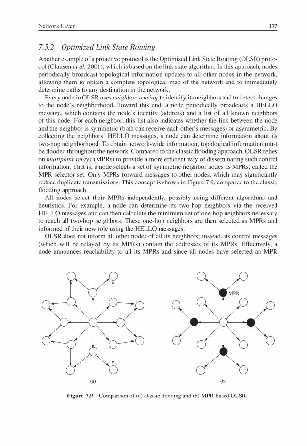
Network Layer 177
7.5.2 Optimized Link State Routing
Another example of a proactive protocol is the Optimized Link State Routing (OLSR) proto-col (Clausen et al. 2001), which is based on the link state algorithm. In this approach, nodesperiodically broadcast topological information updates to all other nodes in the network,allowing them to obtain a complete topological map of the network and to immediatelydetermine paths to any destination in the network.
Every node in OLSR uses neighbor sensing to identify its neighbors and to detect changesto the node’s neighborhood. Toward this end, a node periodically broadcasts a HELLOmessage, which contains the node’s identity (address) and a list of all known neighborsof this node. For each neighbor, this list also indicates whether the link between the nodeand the neighbor is symmetric (both can receive each other’s messages) or asymmetric. Bycollecting the neighbors’ HELLO messages, a node can determine information about itstwo-hop neighborhood. To obtain network-wide information, topological information mustbe flooded throughout the network. Compared to the classic flooding approach, OLSR relieson multipoint relays (MPRs) to provide a more efficient way of disseminating such controlinformation. That is, a node selects a set of symmetric neighbor nodes as MPRs, called theMPR selector set. Only MPRs forward messages to other nodes, which may significantlyreduce duplicate transmissions. This concept is shown in Figure 7.9, compared to the classicflooding approach.
All nodes select their MPRs independently, possibly using different algorithms andheuristics. For example, a node can determine its two-hop neighbors via the receivedHELLO messages and can then calculate the minimum set of one-hop neighbors necessaryto reach all two-hop neighbors. These one-hop neighbors are then selected as MPRs andinformed of their new role using the HELLO messages.
OLSR does not inform all other nodes of all its neighbors; instead, its control messages(which will be relayed by its MPRs) contain the addresses of its MPRs. Effectively, anode announces reachability to all its MPRs and since all nodes have selected an MPR
(a) (b)
MPR
Figure 7.9 Comparison of (a) classic flooding and (b) MPR-based OLSR.
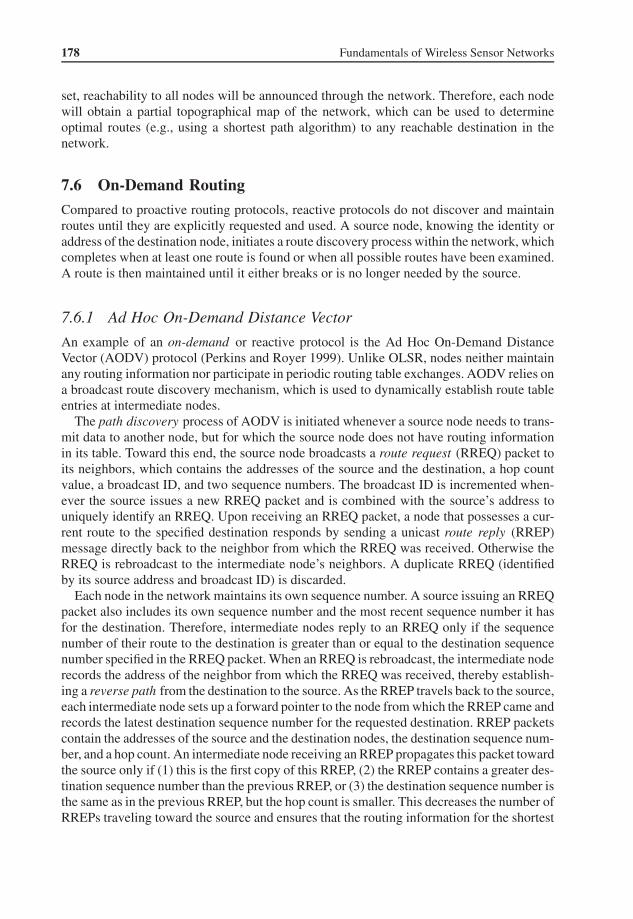
178 Fundamentals of Wireless Sensor Networks
set, reachability to all nodes will be announced through the network. Therefore, each nodewill obtain a partial topographical map of the network, which can be used to determineoptimal routes (e.g., using a shortest path algorithm) to any reachable destination in thenetwork.
7.6 On-Demand Routing
Compared to proactive routing protocols, reactive protocols do not discover and maintainroutes until they are explicitly requested and used. A source node, knowing the identity oraddress of the destination node, initiates a route discovery process within the network, whichcompletes when at least one route is found or when all possible routes have been examined.A route is then maintained until it either breaks or is no longer needed by the source.
7.6.1 Ad Hoc On-Demand Distance Vector
An example of an on-demand or reactive protocol is the Ad Hoc On-Demand DistanceVector (AODV) protocol (Perkins and Royer 1999). Unlike OLSR, nodes neither maintainany routing information nor participate in periodic routing table exchanges. AODV relies ona broadcast route discovery mechanism, which is used to dynamically establish route tableentries at intermediate nodes.
The path discovery process of AODV is initiated whenever a source node needs to trans-mit data to another node, but for which the source node does not have routing informationin its table. Toward this end, the source node broadcasts a route request (RREQ) packet toits neighbors, which contains the addresses of the source and the destination, a hop countvalue, a broadcast ID, and two sequence numbers. The broadcast ID is incremented when-ever the source issues a new RREQ packet and is combined with the source’s address touniquely identify an RREQ. Upon receiving an RREQ packet, a node that possesses a cur-rent route to the specified destination responds by sending a unicast route reply (RREP)message directly back to the neighbor from which the RREQ was received. Otherwise theRREQ is rebroadcast to the intermediate node’s neighbors. A duplicate RREQ (identifiedby its source address and broadcast ID) is discarded.
Each node in the network maintains its own sequence number. A source issuing an RREQpacket also includes its own sequence number and the most recent sequence number it hasfor the destination. Therefore, intermediate nodes reply to an RREQ only if the sequencenumber of their route to the destination is greater than or equal to the destination sequencenumber specified in the RREQ packet. When an RREQ is rebroadcast, the intermediate noderecords the address of the neighbor from which the RREQ was received, thereby establish-ing a reverse path from the destination to the source. As the RREP travels back to the source,each intermediate node sets up a forward pointer to the node from which the RREP came andrecords the latest destination sequence number for the requested destination. RREP packetscontain the addresses of the source and the destination nodes, the destination sequence num-ber, and a hop count. An intermediate node receiving an RREP propagates this packet towardthe source only if (1) this is the first copy of this RREP, (2) the RREP contains a greater des-tination sequence number than the previous RREP, or (3) the destination sequence number isthe same as in the previous RREP, but the hop count is smaller. This decreases the number ofRREPs traveling toward the source and ensures that the routing information for the shortest

Network Layer 179
Path Taken By RREP PacketRREQ Packet Propagation
Source
Destination
Source
Destination
Figure 7.10 Path discovery process of AODV.
route (in terms of number of hops) reaches the source. An example of this path discoveryprocess is shown in Figure 7.10.
A timer for each entry in each node’s routing table limits the lifetime of unused routes.Neighboring nodes also exchange periodic HELLO messages to monitor the state of theirlinks. When a link along the route breaks (e.g., due to a moving node), the intermediate nodecloser to the source noticing the broken link issues a route error (RERR) packet upstreamtoward the source. Upon receiving an RERR packet, a source node can reinitiate the pathdiscovery process.
Using AODV, routes are only established when needed, avoiding costly route tableupdates and exchanges for routes that may never be used. However, AODV does requireperiodic exchanges of HELLO messages among neighbors. Further, since a source nodemay not have a valid route in its table when it wishes to transmit data, there can be an initialdelay (for completion of the path discovery process) before the route can be used. Finally,since the route established from the source to the destination is the reverse path of RREPpackets that traveled from the destination to the source, AODV assumes that all links aresymmetric.
7.6.2 Dynamic Source Routing
The Dynamic Source Routing (DSR) protocol (Johnson 1994) employs route discovery androute maintenance procedures similar to AODV. In DSR, each node maintains a route cachewith entries that are continuously updated as a node learns new routes. Similar to AODV, anode wishing to send a packet will first inspect its route cache to see whether it already hasa route to the destination. If there is no valid route in the cache, the sender initiates a routediscovery procedure by broadcasting a route request packet, which contains the address ofthe destination, the address of the source, and a unique request ID. As this request propagatesthrough the network, each node inserts its own address into the request packet before re-broadcasting it. As a consequence, a request packet records a route consisting of all nodes ithas visited. When a node receives a request packet and finds its own address recorded in thepacket, it discards this packet and does not rebroadcast it further. A node keeps a cache ofrecently forwarded request packets, recording their sender addresses and request IDs, anddiscards any duplicate request packets.
Once a request packet arrives at the destination, it will have recorded the entire path fromthe source to the destination. In symmetric networks, the destination node can unicast a

180 Fundamentals of Wireless Sensor Networks
response packet, containing the collected route information, back to the source using theexact same path as taken by the request packet. In networks with asymmetric links, thedestination can itself initiate a route discovery procedure to the source, where the requestpacket also contains the path from the source to the destination. Once the response packet(or the destination’s request packet) arrives at the source, the source can add the new routeinto its cache and begin transmitting packets to the destination. Similar to AODV, DSRalso employs a route maintenance procedure based on error messages, which are generatedwhenever the link layer detects a transmission failure due to a broken link.
Compared to proactive routing protocols, DSR shares similar advantages and disadvan-tages as AODV. Unlike AODV, each packet in DSR carries route information, which allowsintermediate nodes to add new routes proactively to their own caches. Also, DSR’s supportof asymmetric links is another advantage compared to AODV.
7.7 Hierarchical Routing
Hierarchical routing protocols are based on the grouping of nodes into clusters to addresssome weaknesses of flat routing protocols, most notably scalability and efficiency. The mainidea behind hierarchical routing is that sensor nodes communicate only directly with a leadernode in their own cluster, typically referred to as cluster head . These cluster heads, whichmay be more powerful and less energy-constrained devices than “regular” sensor nodes, arethen responsible for propagating the sensor data to the sink. This approach can significantlyreduce the communication and energy burdens on sensor nodes, while cluster heads willexperience significantly more traffic than regular sensor nodes.
Challenges in the design and operation of hierarchical routing protocols include the selec-tion of cluster heads, the formation of clusters, and adaptations to network dynamics such asmobility or cluster head failures. Compared to flat routing approaches, hierarchical solutionsmay reduce collisions in the wireless medium and facilitate the duty cycling of sensor nodesfor increased energy efficiency. Clustering may also facilitate the routing process, but maylead to longer routes than many flat routing protocols. Clustering also facilitates in-networkaggregation of sensor data, because data coming from colocated sensors (which may monitoroverlapping regions of the environment) are likely to pass through the same cluster head.Figure 7.11 illustrates two variations of the clustering approach. When all cluster headscommunicate directly with the sink node (left graph), the routing challenge is reduced to thecluster formation problem. When cluster heads do not directly communicate with the sink(right graph), a cluster-based routing protocol must also establish multi-hop routes from allcluster heads to the sink.
In the landmark routing technique (Tsuchiya 1988), nodes self-organize into hierarchies,where a landmark is a node to which its neighbors within a certain number of hops knowa route to that node. For example, in the left graph of Figure 7.12, assume that nodes 2–6have routing information for node 1. On the other hand, nodes 7–11 do not have routesto node 1, therefore node 1 is a landmark “visible” to all nodes within a 2-hop distance.Node 1 is then a landmark of radius 2. In general terms, a node i for which all other nodeswithin n hops have routing information toward i is a landmark of radius n. Using this def-inition, a hierarchy of landmarks can be constructed, where a packet can be forwardedtoward a destination by choosing an appropriate sequence of landmarks. The right graphin Figure 7.12 shows an example of such a hierarchy, where the dotted lines and the circles
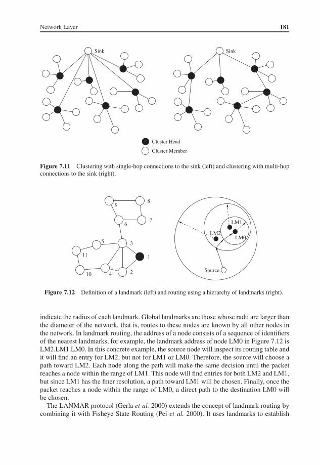
Network Layer 181
Cluster Member
Cluster Head
SinkSink
Figure 7.11 Clustering with single-hop connections to the sink (left) and clustering with multi-hopconnections to the sink (right).
LM2
9
11
5
1
2
3
410Source
LM1
LM0
67
8
Figure 7.12 Definition of a landmark (left) and routing using a hierarchy of landmarks (right).
indicate the radius of each landmark. Global landmarks are those whose radii are larger thanthe diameter of the network, that is, routes to these nodes are known by all other nodes inthe network. In landmark routing, the address of a node consists of a sequence of identifiersof the nearest landmarks, for example, the landmark address of node LM0 in Figure 7.12 isLM2.LM1.LM0. In this concrete example, the source node will inspect its routing table andit will find an entry for LM2, but not for LM1 or LM0. Therefore, the source will choose apath toward LM2. Each node along the path will make the same decision until the packetreaches a node within the range of LM1. This node will find entries for both LM2 and LM1,but since LM1 has the finer resolution, a path toward LM1 will be chosen. Finally, once thepacket reaches a node within the range of LM0, a direct path to the destination LM0 willbe chosen.
The LANMAR protocol (Gerla et al. 2000) extends the concept of landmark routing bycombining it with Fisheye State Routing (Pei et al. 2000). It uses landmarks to establish

182 Fundamentals of Wireless Sensor Networks
a two-tiered logical hierarchy, where each landmark is a cluster head of a logical subnet.Fisheye State Routing is a link state routing protocol, where the frequency of route updatesdepends on the distance, that is, routes within a fisheye scope (a certain predefined distance)are more accurate than routes to more distant nodes. In LANMAR, routing updates are onlyexchanged with nodes in the immediate neighborhood and with landmark nodes; the updatefrequency of all other nodes is zero. When a node needs to relay a packet, the packet willbe forwarded directly to the destination if the destination node is within the node’s fisheyescope. Otherwise, the packet will be forwarded toward the landmark corresponding to thedestination’s logical subnet. Again, once a packet enters the scope of the destination, it isrouted directly to it.
Another hierarchical clustering algorithm is the Low-Energy Adaptive Clustering Hierar-chy (LEACH) protocol (see Section 6.4.5 for protocol details), which combines a clusteringapproach with MAC-layer techniques. LEACH assumes that every cluster head can directlycommunicate with the base station. With LEACH, cluster heads are responsible for all com-munication between their cluster members and a base station and the aggregation of datacoming from its cluster members in order to eliminate redundancies. LEACH can achievesignificant energy savings (depending on how much redundancy can be removed) and sensornodes (apart from the cluster heads) are not responsible for forwarding other nodes’ data.
The main idea of the Power-Efficient Gathering in Sensor Information Systems (PEGA-SIS) protocol (Lindsey and Raghavendra 2002) is for each node to exchange packets withclose neighbors and take turns in being responsible for relaying packets to the base station.Toward this end, nodes organize into a chain, for example, using a greedy algorithm initi-ated by a specific node or computed by the base station, which then broadcasts the chaininformation to all other nodes. While data travels along a chain, it can be aggregated withother data until relayed to the base station. PEGASIS achieves high-energy efficiency sinceeach node only communicates with its closest neighbors (thereby also allowing a node toreduce its transmission power to the lowest required to reach its neighbors in the chain)and occasionally serves as relay toward the base station. Similar to LEACH, the protocolassumes that all nodes can communicate with the base station. A disadvantage in PEGASISis that packets may experience significant delays, particularly if they originate from dis-tant nodes in the chain. Finally, the node serving as relay to the base station can becomea bottleneck.
The Safari architecture (Du et al. 2008) also provides a self-organizing network hierar-chy and a routing protocol with similarity to the landmark approaches. Such landmarks,called drums in Safari, use a self-election algorithm (a distributed algorithm with no cen-tralized coordination) to form subnets, called cells and supercells . At the lowest level of thecell hierarchy (level 0), each individual node forms its own cell. At level 1, Safari definesfundamental cells , that is, cells that contain multiple individual nodes, but no other cells.Higher-level cells are then composed of multiple smaller cells at lower levels. Each drumperiodically broadcasts beacon messages within well-defined limited scopes in the network.These beacons aid the hierarchy formation, give nodes an indication of their position inthe network topology, and provide routing information toward the drum’s cell. Safari usesa hybrid approach for routing, that is, routing within cells is based on the reactive DSRprotocols, while a proactive routing approach is used to compute routes to more distantnodes. The inter-cell communication relies on a destination node’s hierarchical address andon the beacon records stored on each node. Basically, inter-cell communication follows the

Network Layer 183
reverse path of the beacons issued by the cells’ drums. The main advantage of Safari overother approaches is its scalability, due to the hybrid routing approach and the hierarchicaladdressing scheme.
7.8 Location-Based Routing
Location-based or geographic routing can be used in networks where sensor nodes are able todetermine their position using a variety of localization systems and algorithms (see Chapter10 for examples of localization techniques). Instead of topological connectivity information,sensors use geographic information to make forwarding decisions. In unicast location-basedrouting, packets are sent directly to a single destination, which is identified by its location.That is, a sender must be aware not only of its own location, but also the location of the des-tination. This location can be obtained either via querying (e.g., flooding a query to requesta response from the destination containing its location) or a location broker , that is, a ser-vice that maps node identities to locations. In broadcast or multicast location-based routingapproaches, the same packet must be disseminated to multiple destinations. Multicast pro-tocols take advantage of the known destination locations to minimize resource consumptionby reducing redundant links.
The identity of a sensor node is typically less important than its location, that is, datamay be disseminated to all nodes that lie within a certain geographic region. This approachis called geocasting and can, for example, be used to diffuse queries to specific regions ofinterest instead of flooding the entire network, significantly reducing both bandwidth andenergy requirements. Once a packet reaches the desired region, it must be either dissemi-nated (multicast) to all nodes within this region or transmitted to at least one node withinthis region (anycast ).
Typically, location-based routing protocols require that every node in the network knowsits own geographic location and the identities and locations of its one-hop neighbors (e.g.,obtained via periodic beacon messages). The destination is expressed either as the locationof a node (instead of a unique address) or a geographic region. Compared to other routingsolutions, an advantage of location-based routing is that only geographic information isneeded for forwarding decisions and it is not necessary to maintain routing tables or toestablish end-to-end paths between sources and destinations, eliminating the need for controlpackets (apart from the beacon messages among neighbors).
7.8.1 Unicast Location-Based Routing
In unicast location-based routing, the goal is to propagate a packet to a specific node locatedat a position known to the sender. The routing protocol’s responsibility on each node is tomake a local forwarding decision to ensure that a packet moves closer to the destinationwith each hop. An example of this simple procedure is shown in Figure 7.13, where brokencircles indicate the transmission ranges of the forwarding nodes and the arrows indicate theresulting path taken by the packet. In this greedy forwarding approach, it is only requiredthat each node knows its own location and the location of its neighbors, and the sourcemust know the location of the destination. However, this approach carries certain risks.Most importantly, a packet may arrive at a node that does not have any neighbors that couldserve as next hops to bring the packet closer to the destination. To identify and circumvent
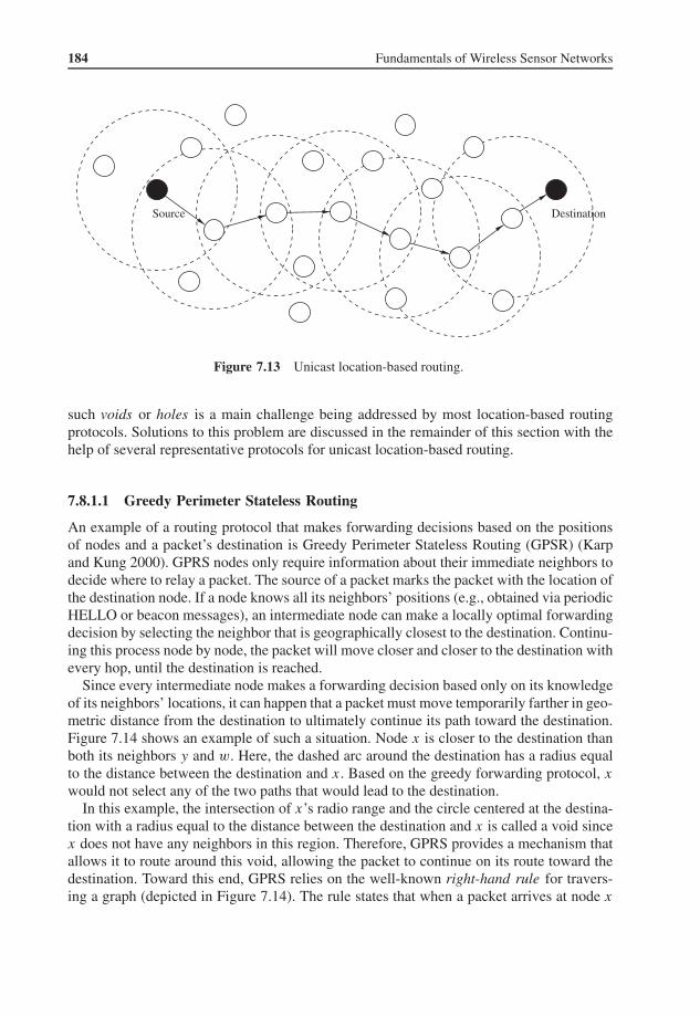
184 Fundamentals of Wireless Sensor Networks
Source Destination
Figure 7.13 Unicast location-based routing.
such voids or holes is a main challenge being addressed by most location-based routingprotocols. Solutions to this problem are discussed in the remainder of this section with thehelp of several representative protocols for unicast location-based routing.
7.8.1.1 Greedy Perimeter Stateless Routing
An example of a routing protocol that makes forwarding decisions based on the positionsof nodes and a packet’s destination is Greedy Perimeter Stateless Routing (GPSR) (Karpand Kung 2000). GPRS nodes only require information about their immediate neighbors todecide where to relay a packet. The source of a packet marks the packet with the location ofthe destination node. If a node knows all its neighbors’ positions (e.g., obtained via periodicHELLO or beacon messages), an intermediate node can make a locally optimal forwardingdecision by selecting the neighbor that is geographically closest to the destination. Continu-ing this process node by node, the packet will move closer and closer to the destination withevery hop, until the destination is reached.
Since every intermediate node makes a forwarding decision based only on its knowledgeof its neighbors’ locations, it can happen that a packet must move temporarily farther in geo-metric distance from the destination to ultimately continue its path toward the destination.Figure 7.14 shows an example of such a situation. Node x is closer to the destination thanboth its neighbors y and w. Here, the dashed arc around the destination has a radius equalto the distance between the destination and x. Based on the greedy forwarding protocol, x
would not select any of the two paths that would lead to the destination.In this example, the intersection of x’s radio range and the circle centered at the destina-
tion with a radius equal to the distance between the destination and x is called a void sincex does not have any neighbors in this region. Therefore, GPRS provides a mechanism thatallows it to route around this void, allowing the packet to continue on its route toward thedestination. Toward this end, GPRS relies on the well-known right-hand rule for travers-ing a graph (depicted in Figure 7.14). The rule states that when a packet arrives at node x
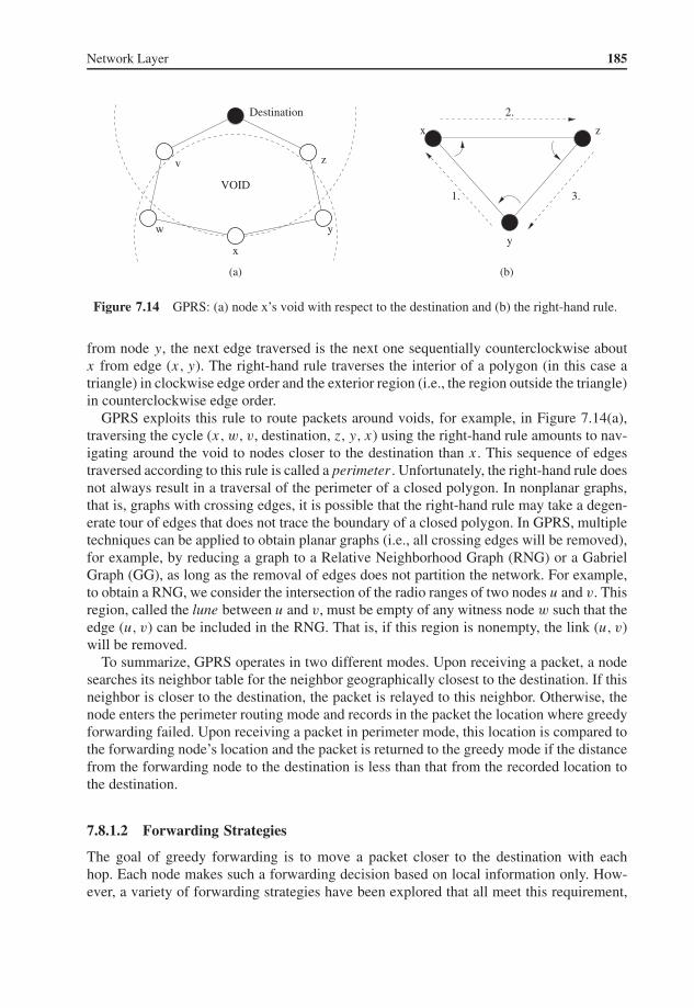
Network Layer 185
(b)
VOID
x
y
z
1.
2.
3.
(a)
w
v z
y
x
Destination
Figure 7.14 GPRS: (a) node x’s void with respect to the destination and (b) the right-hand rule.
from node y, the next edge traversed is the next one sequentially counterclockwise aboutx from edge (x, y). The right-hand rule traverses the interior of a polygon (in this case atriangle) in clockwise edge order and the exterior region (i.e., the region outside the triangle)in counterclockwise edge order.
GPRS exploits this rule to route packets around voids, for example, in Figure 7.14(a),traversing the cycle (x, w, v, destination, z, y, x) using the right-hand rule amounts to nav-igating around the void to nodes closer to the destination than x. This sequence of edgestraversed according to this rule is called a perimeter . Unfortunately, the right-hand rule doesnot always result in a traversal of the perimeter of a closed polygon. In nonplanar graphs,that is, graphs with crossing edges, it is possible that the right-hand rule may take a degen-erate tour of edges that does not trace the boundary of a closed polygon. In GPRS, multipletechniques can be applied to obtain planar graphs (i.e., all crossing edges will be removed),for example, by reducing a graph to a Relative Neighborhood Graph (RNG) or a GabrielGraph (GG), as long as the removal of edges does not partition the network. For example,to obtain a RNG, we consider the intersection of the radio ranges of two nodes u and v. Thisregion, called the lune between u and v, must be empty of any witness node w such that theedge (u, v) can be included in the RNG. That is, if this region is nonempty, the link (u, v)will be removed.
To summarize, GPRS operates in two different modes. Upon receiving a packet, a nodesearches its neighbor table for the neighbor geographically closest to the destination. If thisneighbor is closer to the destination, the packet is relayed to this neighbor. Otherwise, thenode enters the perimeter routing mode and records in the packet the location where greedyforwarding failed. Upon receiving a packet in perimeter mode, this location is compared tothe forwarding node’s location and the packet is returned to the greedy mode if the distancefrom the forwarding node to the destination is less than that from the recorded location tothe destination.
7.8.1.2 Forwarding Strategies
The goal of greedy forwarding is to move a packet closer to the destination with eachhop. Each node makes such a forwarding decision based on local information only. How-ever, a variety of forwarding strategies have been explored that all meet this requirement,
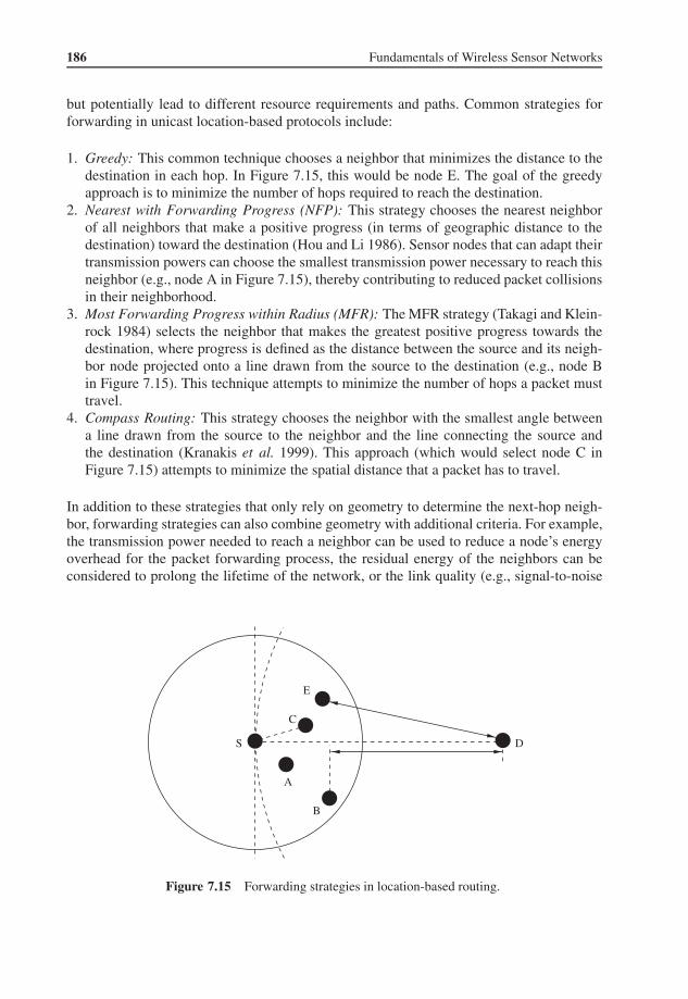
186 Fundamentals of Wireless Sensor Networks
but potentially lead to different resource requirements and paths. Common strategies forforwarding in unicast location-based protocols include:
1. Greedy: This common technique chooses a neighbor that minimizes the distance to thedestination in each hop. In Figure 7.15, this would be node E. The goal of the greedyapproach is to minimize the number of hops required to reach the destination.
2. Nearest with Forwarding Progress (NFP): This strategy chooses the nearest neighborof all neighbors that make a positive progress (in terms of geographic distance to thedestination) toward the destination (Hou and Li 1986). Sensor nodes that can adapt theirtransmission powers can choose the smallest transmission power necessary to reach thisneighbor (e.g., node A in Figure 7.15), thereby contributing to reduced packet collisionsin their neighborhood.
3. Most Forwarding Progress within Radius (MFR): The MFR strategy (Takagi and Klein-rock 1984) selects the neighbor that makes the greatest positive progress towards thedestination, where progress is defined as the distance between the source and its neigh-bor node projected onto a line drawn from the source to the destination (e.g., node Bin Figure 7.15). This technique attempts to minimize the number of hops a packet musttravel.
4. Compass Routing: This strategy chooses the neighbor with the smallest angle betweena line drawn from the source to the neighbor and the line connecting the source andthe destination (Kranakis et al. 1999). This approach (which would select node C inFigure 7.15) attempts to minimize the spatial distance that a packet has to travel.
In addition to these strategies that only rely on geometry to determine the next-hop neigh-bor, forwarding strategies can also combine geometry with additional criteria. For example,the transmission power needed to reach a neighbor can be used to reduce a node’s energyoverhead for the packet forwarding process, the residual energy of the neighbors can beconsidered to prolong the lifetime of the network, or the link quality (e.g., signal-to-noise
S
A
B
D
E
C
Figure 7.15 Forwarding strategies in location-based routing.

Network Layer 187
ratio) can be used to maximize the number of successful packet deliveries and to minimizethe number of required retransmissions.
7.8.1.3 Geographic Adaptive Fidelity
The Geographic Adaptive Fidelity (GAF) protocol (Xu et al. 2001) is another example of anenergy-aware unicast location-based routing protocol, but is primarily designed for networkswith mobile nodes. The network region is divided into a virtual grid, where only a singledevice in each grid cell serves as the forwarding node at any given time. This node is thenresponsible for relaying data to the base station, while all other nodes can go to sleep. Further,GAF assumes that for two adjacent cells A and B, all nodes in A can communicate withall nodes in B and vice versa (Figure 7.16). The grid and cell sizes can be predetermined,allowing each node (assuming that it knows its own location) to determine the cell to which itbelongs. That means that most nodes in the network will have neighbors in all four directions(except nodes in border cells).
Nodes in GAF transit between three different states. Initially, each node enters the dis-covery state, where it listens for messages from other nodes within its cell. It also sets atimer for a certain timeout duration and once the timer fires, the node broadcasts a dis-covery message and enters the active state. The node uses another timer to reenter thediscovery state once that second timer fires. While in the active state, the node periodi-cally rebroadcasts its discovery message. Further, while in either discovery or active state,a node can enter the sleep state whenever it determines that some other node will handlethe forwarding of packets. This is achieved using an application-dependent negotiation pro-cedure, for example, based on the expected lifetime of a node. Nodes in the active statewin the negotiation process over nodes in the discovery mode. In the case of ties, nodeIDs can be used to decide which node will serve as forwarder. In general, the goal of thisapproach is to quickly reach a state where a cell has only one active node. Nodes enteringthe sleep state periodically reenter the discovery state to repeat the process of negotiating theforwarding roles.
Base Station
Figure 7.16 Virtual grid approach of GAF.

188 Fundamentals of Wireless Sensor Networks
7.8.2 Multicast Location-Based Routing
Multicast is used to deliver the same packet to multiple receivers. A simple approach coulddeliver the packet to each receiver separately via unicast routing. However, this approach isresource-inefficient in that it does not exploit the fact that routes to different receivers mayshare paths. Another technique is to simply flood the entire network, which ensures that allreceivers will obtain a copy of the packet, but is also very resource costly. Multicast routingis concerned with the efficient delivery of the same packet to all receivers by minimizingthe number of links the packet has to travel to reach all destinations. A common technique isto establish a multicast tree rooted at the packet source with the destinations as leaf nodes.This section describes representative protocols for multicasts in sensor networks that takeadvantage of geographic information.
The Scalable Position-Based Multicast (SPBM) protocol (Transier et al. 2007) relies ona group management scheme to maintain a list of all destinations for a particular packet.However, instead of putting all destinations into the packet header, SPBM uses hierarchi-cal group membership management to ensure that the approach is efficient even when thenumber of destinations is large. Toward this end, the network is represented as quad-treewith a pre-defined number of levels L, for example, the left graph in Figure 7.17 illustratesan example with L = 4 (levels 0 . . . L−1). Squares are identified by concatenating theirlevel numbers, for example, square 442 is a level-0 square, located in the level-3 square thatencompasses the entire network, the level-2 square 4, and the level-1 square 44. All nodesin a level-0 square are in radio range of each other.
Based on this hierarchical addressing scheme, each node maintains two tables: a globalmember table containing entries for the three neighboring squares for each level and a localmember table containing all members of the node’s level-0 neighbors. Each entry in theglobal member table contains the square’s identifier and a list of nodes located in the square.Each entry in the local member table contains a node ID and the membership informationof that node. This membership information indicates the multicast groups to which a node
442
Level 3
1
2
41
42 43
443
441444
1
2 3 3
41
42 43
Level 0
Level 1
Level 2
443
444
Source
441
442
Figure 7.17 Quad-tree network representation in SPBM (left) and routing using the quad-tree(right).

Network Layer 189
belongs and is encoded as vector where each bit represents a multicast group. For example,an entry of 10100010 for square 41 in the global membership table would indicate that thereexist nodes in square 41 that belong to multicast groups 2, 6, and 8. An entry of 00000001for node 14 in the local membership table indicates that node 14 is a member of multicastgroup 1 only. The contents of a node’s local membership table are periodically broadcastwithin the node’s level-0 square. A randomly chosen node in each level-0 square periodicallydisseminates its global membership table to all nodes in its level-1 square, and this processis repeated for higher-level squares.
Using these tables, a source can now disseminate a packet to all nodes subscribed to amulticast group. For example, in the right graph of Figure 7.17, the source wishes to transmita packet to its multicast group members located in squares 441, 444, and 43 (indicated by theblack circles). Using its global membership table, it knows that there are multicast membersin level-2 square 4 and therefore forwards the packet toward that direction. Similar to GPSR,SPBM uses a greedy forwarding approach by choosing next-hop neighbors that make thelargest progress toward a destination. Once the packet arrives at a node in square 42, thatnode knows that there are multicast members in level-1 squares 43 and 44 and thereforeforwards the packets toward each square. The rule for splitting a multicast packet is based ona heuristic that provides a tradeoff between the total number of nodes forwarding the packetand the optimality of the individual routes toward the destinations. Once a forwarding nodefinds a multicast member in its local membership table, it forwards the packet directly to thatmember node. Similar to GPSR, whenever greedy forwarding fails, the protocol switchesinto perimeter routing mode.
Other location-based multicast protocols are the Geographic Multicast Routing (GMR)protocol (Sanchez et al. 2006) and the Receiver Based Multicast (RBMulticast) protocol(Feng and Heinzelman 2009). GMR uses a heuristic neighbor selection scheme that requireslow computational overheads, resulting in efficient routes based on a cost over progress met-ric. This metric is a ratio of the number of selected forwarding nodes over the progress madetoward all destinations (i.e., the total remaining distance from the neighbors to the destina-tions minus the total distance from the forwarding node to all destinations). RBMulticast isa receiver-based multicast approach, that is, a sender can transmit packets without specify-ing the next-hop node. Similar to SPBM, RBMulticast divides the network into multicastregions , splitting packets depending on the locations of the destinations. However, RBMul-ticast is a completely stateless protocol, eliminating the need for membership tables. Thisis achieved by representing each multicast region with a virtual node and each forwardingnode replicates a packet for each region that contains at least one multicast member. Thedestination of a packet is then the virtual node for a particular multicast region. In RBMul-ticast, it is up to the MAC layer to ensure that the neighbor closest to the location of thevirtual node takes responsibility for forwarding the packet. That is, RBMulticast assumesan underlying MAC protocol where receivers contend for channel access and nodes thatmake the most forward progress to the destination will contend earlier and have a betterchance to become the next-hop node.
7.8.3 Geocasting
In many wireless sensor networks, it is preferred to propagate information to all or somenodes within a specific geographic region. This is a very natural model for many sensor

190 Fundamentals of Wireless Sensor Networks
network applications, specifically when the exact location of individual sensors is unknown.For example, in query-based networks, the same query can be propagated to multiple sen-sors monitoring a specific geographic area, instead of sending the same query repeatedly todifferent individual sensors. The routing problem then consists of two separate challenges:(1) propagating a packet near the target region and (2) distributing a packet within the targetregion. The first challenge can be addressed using approaches similar to unicast location-based routing as previously described, although no exact location of a sensor node near orwithin the target region may be known. If it is sufficient for a packet to reach only a sin-gle node within the target region, the protocol has succeeded once the packet arrives onat least one node within the region. However, if all nodes within the region must obtain acopy of the packet, the second challenge can be addressed using approaches similar to thebroadcast techniques described previously. Therefore, geocasting to multiple receivers is acombination of both unicast and broadcast geographic routing.
7.8.3.1 Geographic and Energy Aware Routing
The Geographic and Energy Aware Routing (GEAR) protocol (Yu et al. 2001) is an exampleof a geocasting protocol, where packets are forwarded to all nodes within a specific targetregion. GEAR consists of the two phases described above: (1) packets are forwarded towardthe target region using a geographical and energy-aware neighbor selection algorithm and(2) packets are disseminated to nodes within the target region using a recursive geographicforwarding algorithm.
Each node in the network maintains two types of costs of reaching a destination viaits neighbors. The estimated cost c(Ni, R) for each neighbor Ni and a target region R isdefined as:
c(Ni, R) = αd(Ni, R) + (1 − α)e(Ni) (7.2)
where α is a tunable weight, d(Ni, R) is the distance from neighbor Ni to the centroidD of region R normalized by the largest such distance among all neighbors, and e(Ni) isthe consumed energy at node Ni , normalized by the largest consumed energy among allneighbors. That is, the estimated cost is a combination of both residual energy and distanceto the target region. The learned cost h(N, R) of a node N is then a refinement of theestimated cost that allows nodes to circumvent voids or holes in the network (if there are noholes, the learned cost and the estimated cost are identical). Similar to GPSR, GEAR makeslocally greedy forwarding decisions, that is, whenever a node receives a packet, it will pickthe next hop among the neighbors that are closer to the destination.
When a node N receives a packet, and if there are no neighbors that are closer to thedestination, N knows that it is in a hole. In this case, the learned cost function is used toselect one of N’s neighbors as the next hop, that is, the packet is forwarded to the node withthe minimum learned cost (ties are broken using some predefined ordering). After a nodepicks the next-hop neighbor Nmin, it sets its own learned cost h(N,R) to h(Nmin, R) +C(N, Nmin), where C(x, y) is the cost of transmitting a packet from node x to node y.Therefore, the learned cost will increase, which allows upstream nodes to avoid forwardingpackets toward the node in the hole. Figure 7.18(a) shows an example of this procedure,where T represents the centroid of the target region. Node S wishes to forward a packettoward the destination and it has three neighbors that are closer to the destination: B, A, and

Network Layer 191
S
F
ABC
D
E
G
HI
T
(b)
S
(a)
Figure 7.18 GEAR: (a) learning routes around holes and (b) recursive geographic forwarding.
I. B’s and I’s learned and estimated costs are√
5 and A’s learned and estimated costs are both2. S will forward the packet to the lowest cost neighbor, which is A. Node A will find itselfin a hole and it will forward the packet to the neighbor with the minimum learned cost, forexample, node B. Additionally, it will update its own cost h(A, T ) = h(B, T ) + C(A, B),that is, assuming a cost (A, B) = 1, the new learned cost of A will be
√5 + 1. The next
time a packet for T arrives at node S, S will forward the packet directly to B instead of A tocircumvent the hole.
Once a packet reaches the target region R, a simple flooding with duplicate suppressionscheme could be used to disseminate the packet to all nodes within R. However, due tothe cost of flooding, GEAR relies on a process called Recursive Geographic Forwarding ,shown in Figure 7.18(b). Assume that the target region R is the large rectangle and nodeS received a packet for R and finds itself within R. Then, S creates four new copies of thepacket bound to four smaller subregions (shown as the smaller rectangles) of region R. Foreach subregion, GEAR repeats the forwarding and splitting process until a packet reaches anode that is the only one within the current subregion.
7.8.3.2 Geographic-Forwarding-Perimeter-Geocast
Another protocol that combines geographic routing with region flooding is the Geographic-Forwarding-Perimeter-Geocast (GFPG) protocol (Seada and Helmy 2004). Similar toGPRS, it uses greedy forwarding to propagate a packet toward its geocast region, wherethe destination is the center of the geocast region. When greedy forwarding fails, perimeterrouting is used to circumvent voids. Once the packet enters the geocast region, simpleflooding could be used to deliver it to all nodes with the region. However, this assumes thatthere are no obstacles and gaps, that is, all nodes within the region must be able to reacheach other without going out of the region. If this assumption does not hold, delivery cannotbe guaranteed. Therefore, GFPG uses a combination of geocast and perimeter routing toguarantee delivery to all nodes. For example, the gray geocast region in Figure 7.19 hastwo clusters of nodes that cannot directly reach each other within the geocast region (i.e.,there is a gap between two nodes in the lower left and the upper right corners).

192 Fundamentals of Wireless Sensor Networks
Source Source
Figure 7.19 An example of a geocast region with a gap (left) and region flooding and perimeterrouting used by GFPG to reach all nodes in the geocast region (right).
Once a packet reaches a geocast region, it is flooded to all nodes, but in addition, regionborder nodes , that is, nodes that have at least one neighbor outside the region, also send thepacket to their neighbors outside the region in the planar graph. Nodes outside the regionforward the packet using the right-hand rule to neighbors in the planar graph and, as a conse-quence, the packet travels around the face until it enters the region again (Figure 7.19). Thefirst node inside the region to receive the perimeter packet floods this packet to its neighborsif it has not seen this packet before. Perimeter routing is therefore able to link disconnectedclusters of a geocast region together.
7.9 QoS-Based Routing Protocols
Although most routing and data dissemination protocols aim for some kind of Quality-of-Service (QoS), for example, minimum hop routing protocols try to achieve low latenciesby using “short” paths, some protocols proposed for sensor networks explicitly addressone or more QoS routing metrics. The goal of these protocols is to find feasible pathsbetween sender and destination, while satisfying one or more QoS metrics (latency, energy,bandwidth, reliability), but also optimizing the use of the scarce network resources. Wire-less sensor networks pose numerous challenges to providing satisfactory QoS, includingdynamic topologies, resource scarcity (including power limitations), varying quality of theradio channels, the lack of centralized control, and the heterogeneity of network devices.This section introduces several representative QoS-based routing protocols for ad hoc andsensor networks.
7.9.1 Sequential Assignment Routing
One of the first routing protocols to explicitly consider Quality-of-Service is the SequentialAssignment Routing (SAR) protocol (Sohrabi et al. 2000), which is also an example of amultipath routing approach. SAR creates multiple trees, each rooted at a 1-hop neighbor of
Network Layer 193
the sink, to establish multiple paths from each node to the sink. These trees grow outwardfrom the sink, while avoiding nodes with low QoS (e.g., high delay). The QoS associatedwith a path is expressed as an additive QoS metric where higher values imply lower QoS.After the tree-building procedure has completed, it is likely that a node is part of multipletrees, that is, it can choose from multiple routes toward the sink. SAR selects a route for apacket based on the QoS metric, energy (in terms of number of packets that can be trans-mitted without energy depletion, assuming exclusive use of the path), and the priority levelof the packet. The goal of SAR is to minimize the average weighted QoS metric over thelifetime of the network. The availability of multiple routes ensures fault-tolerance and quickrecovery from broken paths. However, establishing and maintaining the trees (i.e., routingtables) are expensive tasks, particularly in large sensor networks.
7.9.2 SPEED
Numerous wireless sensor applications require sensor data collection within certain timeconstraints to ensure that the collected information is useful and can be acted upon in atimely fashion. For example, events of interest such as the detection of moving objects insurveillance systems or the impending failure of a bridge require rapid responses.
For applications with soft real-time requirements, SPEED (He et al. 2003) is anexample of a protocol that provides real-time communication services, including real-timeunicast, real-time area-multicast, and real-time area-anycast. SPEED is also an example of alocation-based routing protocol, that is, a node relies on position information from its neigh-bors instead of routing tables. Position information is obtained through periodic HELLO (orbeacon) messages that contain a node’s ID, position, and an average receive delay. Each nodealso maintains a neighbor table containing the node ID and position for each of its neighbors,but also an expiration time (ExpireTime) and two delays called ReceiveFromDelay andSendToDelay. The SendToDelay is the delay received from the beacon message comingfrom the neighbor, while the ReceiveFromDelay is estimated by measuring the delay expe-rienced by a packet in the MAC layer of the sender plus a propagation delay. The Receive-FromDelay values of all neighbors are averaged periodically to obtain a single receive delay.
The routing component of the SPEED protocol is called Stateless Nondeterministic Geo-graphic Forwarding (SGNF). The neighbor set of a node i is defined as the set of neighborsof i (i.e., all nodes within i’s radio range) that are at least a distance of K away from i. Theforwarding candidate set (FSDest
i ) of a node i for destination Dest consists of all nodes fromthe node’s neighbor set that are at least a distance of K closer to the destination. That is,if L is the distance of node i from the destination and Lnext is the distance from i’s neigh-bor j to the destination, L − Lnext has to be greater than or equal to K in order to add j toi’s forwarding candidate set. Packets are only forwarded to nodes belonging to FSDest
i andif this set is empty, packets are dropped. SPEED further divides the forwarding candidateset into two subsets: one contains nodes that have a SendToDelay less than a certain singlehop delay D, and the other contains the remaining nodes. The forwarding candidate is thenselected from the first group where nodes with higher relay speed have a greater chance ofbeing chosen. The relay speed considers both distance and delays and is calculated as:
RelaySpeed = |L − Lnext|SendToDelay
(7.3)

194 Fundamentals of Wireless Sensor Networks
where a discrete exponential distribution can be used to trade off between load balancing andoptimal path length. If there are no nodes in the first subset of forwarding candidates, a relayratio is calculated, based on another component of the SPEED protocol, the neighborhoodfeedback loop. This component is responsible for determining the relay ratio by lookingat the miss ratios of the neighbors of a node (i.e., the nodes which could not provide therequired RelaySpeed). If this relay ratio is less than a randomly generated number between0 and 1, the packet is dropped. The goal of the neighborhood feedback loop is to keep thesystem performance at a desired value, that is, it attempts to maintain a single hop delaybelow a certain value D.
The final component of SPEED is the back-pressure rerouting protocol, which is respon-sible for (i) preventing voids that occur when a node fails to find a next hop node and (ii)reducing congestion using a feedback approach. Figure 7.20 depicts two examples show-ing the operation of this technique. In both examples, the shaded regions are areas wheretraffic is high, causing congestion. In the first case, node 3 will be notified of the delaysexperienced by nodes 6 and 7 through the beacon exchange process. The SGNF compo-nent of SPEED reduces the probability of nodes 6 and 7 being selected as forwardingnodes, therefore reducing the congestion around these nodes. In the second case, all for-warding nodes of 3 are congested and, in this case, both the neighborhood feedback loopand SGNF work together to address the congestion. For example, node 3 may drop a cer-tain number of packets, where these dropped packets count as packet with delay D in termsof computing the delay at this node. The average delay of 3 will increase, which will bedetected by 3’s upstream nodes (i.e., node 2). Should node 2 be in the same situation asnode 3, further back-pressure will be imposed on node 1, that is, back-pressure reroutingmay continue to proceed upstream until it reaches the source, which can then suppressfurther packets.
7.9.3 Multipath Multi-SPEED
The goal of the Multipath Multi-SPEED (MMSPEED) protocol (Felemban et al. 2006) isto provide QoS differentiation in terms of timeliness and reliability , while at the same time
Case 1 Case 2
318
2’s Neighbor Table
DROP: Delay
6
2
3
7
8
9
4
1
Delay
Congestion
Node Delay
0.0 −> 0.5 > D0.1 −> 0.1 < D0.1 −> 0.1 < D
Node
6472
3’s Neighbor Table
1
3
4
6
7 Delay
Congestion
Delay
0.0 −> 0.5 > D0.1 −> 0.1 < D0.0 −> 0.4 > D0.1 −> 0.1 < D
2
5
Figure 7.20 Two examples of back-pressure rerouting in SPEED.

Network Layer 195
loss
physical
network
logical
low-speed
network
logical
high-speed
network
high
reliability
low
reliability
loss
source destination source destination
Figure 7.21 Service differentiation in the latency domain (left) and the reliability domain (right).
minimizing the protocol’s overhead by making localized routing decisions without a pri-ori route discovery or global network state updates. Similar to SPEED, the protocol relieson geographic locations of nodes to make forwarding decisions, where these locations areexchanged among neighboring nodes using periodic beacon messages.
With respect to timeliness, MMSPEED offers packets multiple delivery speed optionsthat are guaranteed throughout the network. Conceptually, this protocol can be understoodas a virtual overlay of multiple SPEED layers on top of a single physical layer (left graphin Figure 7.21). Each layer l is associated with a SetSpeedl, which is a prespecified lower-bound speed. That is, when a node computes the relay speed for each of its neighbors (seeSection 7.9.2), it then chooses a forwarding neighbor whose relay speed is at least the desiredSetSpeed value. For example, assume that the minimum required speed level ReqSpeed(x)for packet x can be calculated as
ReqSpeed(x) = dists,d(x)
deadline(x)(7.4)
where dists,d is the distance from the source s to the destination d for packet x with a given(end-to-end) deadline(x). Then, the speed layer l for the packet is selected such that
SetSpeedl = minLj=1{SetSpeedj |SetSpeedj ≥ ReqSpeed(x)} (7.5)
where L is the number of available speed options. In this case, the node chooses a neigh-bor i whose progress speed estimation RelaySpeed = |dists,d − disti,d |/delays,i is at leastSetSpeedl . It is possible that a packet’s delays over a route differ from the delay estimations.Therefore, the layer selected at one node can differ from the layer selected at another node,for example, a slow packet can be boosted by using a higher layer at a subsequent node.Toward this end, it is necessary to determine a packet’s remaining time to its deadline, whichrequires synchronized clocks in the network. Instead, MMSPEED measures the elapsed timeat each node and piggybacks this information onto a packet such that subsequent nodes candetermine the remaining time to the deadline.
Similarly, MMSPEED offers packets multiple levels of reliability. Toward this end, itexploits the fact that there exist multiple redundant paths from a source to a destination,even though these paths will differ in length and QoS (right graph in Figure 7.21). Each

196 Fundamentals of Wireless Sensor Networks
node i maintains the recent average of packet loss percentage ei,j to each neighbor j . Suchlosses include both intentional packet drops for congestion control and errors in the wirelesschannel. Based on these averages, a node computes an estimate of packet loss probabilitybetween itself and a packet’s destination as
RPdi,j = (1 − ei,j )(1 − ei,j )
�distj,d/disti,j � (7.6)
where �distj,d/disti,j� is the hop count estimation from node j to the destination d . Thisestimation is based on the assumption that subsequent nodes have a similar packet loss rateto node i and that the progress to the destination for each following hop will be similarto the current progress. Based on this computation, a node can determine the number offorwarding paths that satisfy the end-to-end reachability requirement of a packet. The totalreaching probability (TRP) is originally set to zero and updated for each forwarding paththat is being used, that is, the TRP is computed as
TRP = 1 − (1 − TRP)(1 − RPdi,j ) (7.7)
Here, (1 − TRP) is the probability that none of the current paths can successfully deliverthe packet to the destination and (1 − RPd
i,j ) is the probability that the additional path willfail to deliver the packet. Therefore, the newly computed TRP is the probability that at leastone path will successfully deliver the packet to the destination. A node adds paths to thisTRP estimation until TRP becomes larger than the required end-to-end reachability P req.
Both latency and reliability considerations can also be combined in MMSPEED. In thiscase, the protocol identifies the required speed level for a given packet and then it findsmultiple forwarding nodes among those with sufficient progress speed such that the totalreaching probability is at least as high as the required reaching probability.
7.10 Summary
While routing in general is a crucial component of any multi-hop network, routing is par-ticularly challenging in wireless ad hoc and sensor networks due to their characteristicssuch as stringent resource constraints and unreliability of links and nodes. Specifically,routing protocols must operate efficiently to avoid premature exhaustion of the limitedresources in a sensor network (most notably energy) and they must be able to adjust to chang-ing and unpredictable network characteristics, including changes in the network topologyand density. In this section, several classes of routing strategies (data-centric, hierarchi-cal, location-based) and numerous examples of concrete routing protocols have been dis-cussed. Table 7.1 summarizes some key characteristics of the protocols discussed in thischapter.
Although numerous routing solutions for sensor networks exist, the unique challengesand the many varieties of network deployment scenarios indicate that there still remaina variety of challenges, for example, with respect to resource efficiency and provision ofQoS. For example, in the recent past, there has been an increased focus on wireless sensornetworks that can support application-specific QoS requirements involving multiple perfor-mance metrics. Other areas of investigation of routing protocols for future sensor networksinclude the need for energy-efficient solutions that make localized decisions, protocols thateffectively exploit redundancy for efficiency and reliability, protocols for newly emerging

Network Layer 197
Table 7.1 Network protocols summary
Protocol Characteristics
SPIN Flat topology, data-centric, query-based, negotiation-basedDirected diffusion Flat topology, data-centric, query-based, negotiation-basedRumor routing Flat topology, data-centric, query-basedGBR Flat topology, data-centric, query-basedDSDV Flat topology with proactive route discoveryOLSR Flat topology with proactive route discoveryAODV Flat topology with reactive route discoveryDSR Flat topology with reactive route discoveryLANMAR Hierarchical with proactive route discoveryLEACH Hierarchical, support of MAC layerPEGASIS HierarchicalSafari Hierarchical, hybrid route discovery (reactive near, proactive remote)GPSR Location-based, unicastGAF Location-based, unicastSPBM Location-based, multicastGEAR Location-based, geocastGFPG Location-based, geocastSAR Flat topology with QoS (real-time, reliability), multipathSPEED Location-based with QoS (real-time)MMSPEED Location-based with QoS (real-time, reliability)
topologies (e.g., architectures with multiple tiers), security-aware routing protocols, andintegrated solutions to routing and in-network processing of sensor data.
Exercises
7.1 The previous chapter presented several MAC protocols, while this chapter introducedrouting protocols. Can you think of examples how the choice of MAC protocol affectsthe design, performance, and efficiency of the routing protocol?
7.2 What is the difference between a proactive routing protocol and a reactive routingprotocol? Name at least two examples for each category. Consider the following WSNscenarios and explain why you would choose either a proactive or a reactive routingsolution:
(a) A WSN is used to monitor air pollution in a city where every sensor reports itssensor data once every minute to a single remote base station. Most sensors aremounted on lamp posts, but some are also mounted on city buses.
(b) A WSN is used to measure humidity in a field, where low-power sensors reportmeasurements only when certain thresholds are exceeded.
(c) A WSN is used to detect the presence of vehicles, where each sensor locallyrecords the times of vehicle detection. These records are delivered to the basestation only when the sensor is explicitly queried.
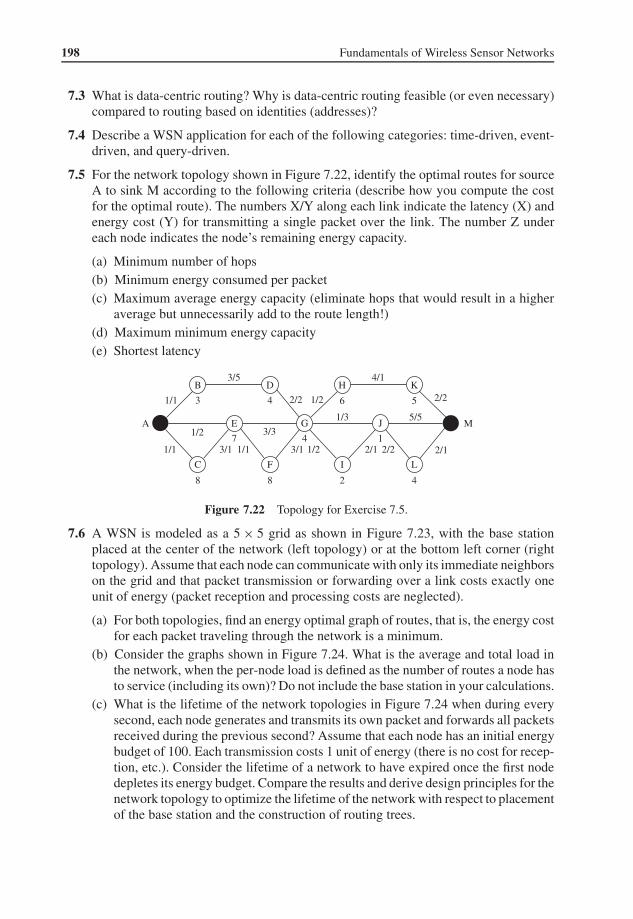
198 Fundamentals of Wireless Sensor Networks
7.3 What is data-centric routing? Why is data-centric routing feasible (or even necessary)compared to routing based on identities (addresses)?
7.4 Describe a WSN application for each of the following categories: time-driven, event-driven, and query-driven.
7.5 For the network topology shown in Figure 7.22, identify the optimal routes for sourceA to sink M according to the following criteria (describe how you compute the costfor the optimal route). The numbers X/Y along each link indicate the latency (X) andenergy cost (Y) for transmitting a single packet over the link. The number Z undereach node indicates the node’s remaining energy capacity.
(a) Minimum number of hops(b) Minimum energy consumed per packet(c) Maximum average energy capacity (eliminate hops that would result in a higher
average but unnecessarily add to the route length!)(d) Maximum minimum energy capacity(e) Shortest latency
1/1
3/3
3/5
3/1 1/11/1 3/1
1/3
1/2
1/22/2
4/1
C
D
E
F
G
I
H
L
J
2/1 2/2 2/1
2/2
8
7
8
3
A
2
6
4
141/2
5/5
B K
M
4 5
Figure 7.22 Topology for Exercise 7.5.
7.6 A WSN is modeled as a 5 × 5 grid as shown in Figure 7.23, with the base stationplaced at the center of the network (left topology) or at the bottom left corner (righttopology). Assume that each node can communicate with only its immediate neighborson the grid and that packet transmission or forwarding over a link costs exactly oneunit of energy (packet reception and processing costs are neglected).
(a) For both topologies, find an energy optimal graph of routes, that is, the energy costfor each packet traveling through the network is a minimum.
(b) Consider the graphs shown in Figure 7.24. What is the average and total load inthe network, when the per-node load is defined as the number of routes a node hasto service (including its own)? Do not include the base station in your calculations.
(c) What is the lifetime of the network topologies in Figure 7.24 when during everysecond, each node generates and transmits its own packet and forwards all packetsreceived during the previous second? Assume that each node has an initial energybudget of 100. Each transmission costs 1 unit of energy (there is no cost for recep-tion, etc.). Consider the lifetime of a network to have expired once the first nodedepletes its energy budget. Compare the results and derive design principles for thenetwork topology to optimize the lifetime of the network with respect to placementof the base station and the construction of routing trees.

Network Layer 199
(d) Assume that the first topology in Figure 7.24 is used and each sensor transmitsexactly one packet to the base station. Then the topology is switched to the secondone and each sensor transmits one packet to the base station in the bottom left cor-ner. Then the topology is switched back to the first one and the process is repeated.Explain why the network lifetime changes and what other design principle can bederived from this insight. (To facilitate the comparison, focus on the case whereeach node has already reached its maximum load.)
Base Station
Sensor Node
Figure 7.23 Topologies for Exercise 7.6.
Base Station
Sensor Node
Figure 7.24 Topologies and routes for Exercise 7.6.
7.7 Flooding is a simple strategy for distributing data to one specific node or all sensornodes in a network. Answer the following questions:
(a) Explain the three challenges of flooding described in this chapter.(b) Which of these can be addressed by gossiping and how can they be addressed?

200 Fundamentals of Wireless Sensor Networks
(c) For the topologies shown in Figure 7.22 and Figure 7.23, what are good choicesfor the maximum hop count? Explain your answer.
(d) How do sequence numbers contribute to reducing unnecessary transmissions? Aresequence numbers alone sufficient and, if not, what other information is needed touse them correctly?
7.8 Using the topology in Figure 7.22, explain the problems of implosion, overlap, andresource blindness.
7.9 How does the SPIN family of protocols address the three challenges faced by flooding?What are the disadvantages of a negotiation-based protocol such as SPIN?
7.10 Explain the concept of directed diffusion. Can you imagine at least three strategies orgoals for reinforcement?
7.11 Consider the network topology in Figure 7.22 and node G’s routing table shown inTable 7.2.
(a) Describe how node G would send queries toward events E1, E2, and E3 usingrumor routing (note that node G has no routing table entries for event E3).
(b) Assume that (i) I informs G that I can reach event E2 via 2 hops, (ii) F informs Gthat F can reach event E3 via 4 hops, (iii) E informs G that E can reach event E1via 1 hop, (iv) D informs G that D can reach event E1 via 2 hops, (v) H informs Gthat H can reach event E2 via 2 hops, and (vi) D informs G that D can reach eventE3 via 1 hop. What is the final table of node G? Can you identify the locations ofall three events by the identity of the closest sensor?
Table 7.2 G’s routing table (Exercise 7.11)
Event Distance Direction
E1 3 FE2 4 I
7.12 What are the concepts behind distance vector routing and link state routing and how dothey compare to each other with respect to overheads for maintaining routing tables?
7.13 Compare a proactive routing protocol such as DSDV with a reactive protocol such asDSR with respect to overheads and route optimality.
7.14 Does DSR incur larger or smaller overheads for route discovery compared to theAODV protocol? Justify your answer.
7.15 In AODV, is it possible that route discovery packets travel in the network forever?Why or why not?
7.16 Asymmetric (or unidirectional) links occur when node A can hear node B, but B cannothear node A. Explain whether this is a problem for the AODV protocol and if so, howthis can be addressed.

Network Layer 201
7.17 What is the concept behind hierarchical routing and what advantages does it have overother techniques?
7.18 Table 7.3 summarizes the routing information of all nodes in a WSN, that is, eachrow indicates the routing knowledge of that particular node. For example, the first rowshows that node A knows that it can reach nodes B and C via 1 hop and nodes D andE via 2 hops. Given this information, draw the network topology and determine thelandmark radius for each node.
Table 7.3 Routing information for Exercise 7.18
A B C D E F G H
A 0 1 1 2 2 – – –B 1 0 1 1 1 2 – –C 1 1 0 2 1 – 2 –D – 1 2 0 1 1 2 2E 2 1 1 1 0 – 1 –F – 2 – 1 2 0 1 1G – 2 2 2 1 1 0 1H – – 3 2 – 1 1 0
7.19 What is the advantage of using Fisheye State Routing in the LANMAR protocol com-pared to the basic landmark routing technique?
7.20 Figure 7.25 shows a number of nodes as small dots. Each node has a radio range of 2units. How would the gray node positioned at (0, 0) route a packet to the gray node atposition (9, 9) using GPSR? Indicate the visited nodes.
(0,0)
Figure 7.25 GPSR routing example (Exercise 7.20).
7.21 When does GPSR enter the perimeter routing mode and how does it use the right-handrule in this mode?

202 Fundamentals of Wireless Sensor Networks
7.22 Prove that it is false or show an example that the perimeter mode can cause a packetto traverse a network’s entire outer boundary.
7.23 Consider the topology in Figure 7.26. Node A wishes to forward a packet toward desti-nation L via one of its neighbors (its communication range is indicated with the circle).Which neighbor will A choose with each of the following forwarding strategies:
(a) greedy forwarding(b) nearest with forwarding progress(c) most forwarding progress within radius(d) compass routing
D
A
B
C
E
LF
I
J
K
H
G
Figure 7.26 Forwarding strategies in GPSR (Exercise 7.23).
7.24 The cell size of the GAF virtual grid can be predetermined and each node knows towhich cell it belongs. Discuss the consequences of choosing very large versus verysmall cell sizes.
7.25 How does the SPBM protocol ensure efficient multicast for large numbers of receivers?
7.26 What is the concept of RBMulticast and how does it address the shortcomings of theSPBM protocol?
7.27 The GEAR protocol uses two types of costs: learned and estimated. Explain howlearned costs are used to route packets around holes (use a concrete example). Whatis the purpose of the estimated costs and what is the intuition behind calculating themas described in this chapter?
7.28 Figure 7.27 shows a sensor network topology, where each node’s transmission rangeis two units. The node at position (0,0) wants to disseminate a packet to all nodeswithin the rectangle. Show how GFPG routes the packet toward the region and how itdistributes it to all receivers within the rectangle. Clearly indicate which nodes (insideand outside the geocast region) will receive the packet.
7.29 Answer the following questions with respect to QoS-aware routing protocols:
(a) What advantages and disadvantages does multipath routing have?(b) How does the SGNF component of SPEED work?

Network Layer 203
(0,0)
Figure 7.27 Geocast region with hole (Exercise 7.28).
(c) How does the back-pressure rerouting component of SPEED work?(d) Why does MMSPEED change the speed of packets as they travel along a route?(e) How can latency and reliability considerations be combined in MMSPEED?
ReferencesAl-Karaki, J.N., and Kamal, A.E. (2004) Routing techniques in wireless sensor networks: A survey. IEEE Wireless
Communications 11 (6), 6–28.Braginsky, D., and Estrin, D. (2002) Rumor routing algorithm for sensor networks. Proc. of the 1st ACM Inter-
national Workshop on Wireless Sensor Networks and Applications .Clausen, T., Hansen, G., Christensen, L., and Behrmann, G. (2001) The optimized link state routing protocol,
evaluation through experiments and simulation. Proc. of the IEEE Symposium on Wireless Personal MobileCommunications .
Couto, D.D., Aguayo, D., Bicket, J., and Morris, R. (2003) High throughput path metric for multi-hop wirelessrouting. Proc. of the 9th Annual International Conference on Mobile Computing and Networking (MobiCom).
Draves, R., Padhye, J., and Zill, B. (2004) Routing in multi-radio, multi-hop wireless mesh networks. Proc. of the10th Annual International Conference on Mobile Computing and Networking (MobiCom).
Du, S., Khan, A., Pal-Chaudhuri, S., Post, A., Saha, A.K., Druschel, P., Johnson, D.B., and Riedi, R. (2008) Safari:A self-organizing, hierarchical architecture for scalable ad hoc networking. Ad Hoc Networks 6 (4), 485–507.
Felemban, E., Lee, C.G., and Ekici, E. (2006) MMSPEED: Multipath multi-SPEED protocol for QoS guaranteeof reliability and timeliness in wireless sensor networks. IEEE Transactions on Mobile Computing 5 (6),738–754.
Feng, C.H., and Heinzelman, W.B. (2009) RB Multicast: Receiver based multicast for wireless sensor networks.Proc. of the IEEE Wireless Communications and Networking Conference (WCNC).
Gerla, M., Hong, X., and Pei, G. (2000) Landmark routing for large ad hoc wireless networks. Proc. of the IEEEGlobal Communications Conference (GLOBECOM).
He, T., Stankovic, J.A., Lu, C., and Abdelzaher, T. (2003) SPEED: A real-time routing protocol for sensor net-works. Proc. of the International Conference on Distributed Computing Systems.
Hedetniemi, S.H., Hedetniemi, S.T., and Liestman, A.L. (1988) A survey of gossiping and broadcasting in com-munication networks. Networks 18 (4), 319–349.
Heinzelman, W., Kulik, J., and Balakrishnan, H. (1999) Adaptive protocols for information dissemination inwireless sensor networks. Proc. of the 5th ACM/IEEE International Conference on Mobile Computing andNetworking (MobiCom).
Hou, T., and Li, V. (1986) Transmission range control in multi-hop packet radio networks. IEEE Transactions onCommunications 34 (1), 38–44.

204 Fundamentals of Wireless Sensor Networks
Intanagonwiwat, C., Govindan, R., and Estrin, D. (2000) Directed diffusion: A scalable and robust communicationparadigm for sensor networks. Proc. of the 6th Annual International Conference on Mobile Computing andNetworking (MobiCom).
Johnson, D.B. (1994) Routing in ad hoc networks of mobile hosts. Proc. of the IEEE Workshop on Mobile Com-puting Systems and Applications .
Karp, B., and Kung, H.T. (2000) GPSR: Greedy perimeter stateless routing for wireless networks. Proc. of the 6thAnnual International Conference on Mobile Computing and Networking (MobiCom).
Kranakis, E., Singh, H., and Urrutia, J. (1999) Compass routing on geometric networks. Proc. of the 11th CanadianConference on Computational Geometry .
Kulik, J., Heinzelman, W., and Balakrishnan, H. (2002) Negotiation-based protocols for disseminating informationin wireless sensor networks. Wireless Networks 8 (2/3), 169–185.
Lindsey, S., and Raghavendra, C.S. (2002) PEGASIS: Power-efficient gathering in sensor information systems.Proc. of the IEEE Aerospace Conference.
Pei, G., Gerla, M., and Chen, T.W. (2000) Fisheye state routing in mobile ad hoc networks. Proc. of the ICDCSWorkshop on Wireless Networks and Mobile Computing .
Perkins, C.E., and Bhagwat, P. (1994) Highly dynamic destination-sequenced distance-vector routing (DSDV) formobile computers. ACM SIGCOMM Computer Communication Review 23 (4), 234–244.
Perkins, C.E., and Royer, E.M. (1999) Ad hoc on-demand distance vector routing. Proc. of the 2nd IEEE Workshopon Mobile Computing Systems and Applications .
Sanchez, J.A., Ruiz, P.M., and Stojmenovic, I. (2006) GMR: Geographic multicast routing for wireless sensornetworks. Proc. of the 3rd Annual IEEE Communications Society Conference on Sensor, Mesh and Ad HocCommunications and Networks .
Schurgers, C., and Srivastava, M.B. (2001) Energy efficient routing in wireless sensor networks. Proc. of the IEEEMilitary Communications Conference (MILCOM).
Seada, K., and Helmy, A. (2004) Efficient geocasting with perfect delivery in wireless networks. Proc. of theIEEE Wireless Communications and Networking Conference (WCNC).
Singh, S., Woo, M., and Raghavendra, C.S. (1998) Power-aware routing in mobile ad hoc networks. Proc. of the4th Annual International Conference on Mobile Computing and Networking (MobiCom).
Sohrabi, K., Gao, J., Ailawadhi, V., and Pottie, G. (2000) Protocols for self-organization of a wireless sensornetwork. IEEE Personal Communications 7 (5), 16–27.
Takagi, H., and Kleinrock, L. (1984) Optimal transmission ranges for randomly distributed packet radio terminals.IEEE Transactions on Communications 32 (3), 246–257.
Transier, M., Fussler, H., Widmer, J., Mauve, M., and Effelsberg, W. (2007) A hierarchical approach to position-based multicast for mobile ad hoc networks. Wireless Networks 13 (4), 447–460.
Tsuchiya, P.F. (1988) The landmark hierarchy: A new hierarchy for routing in very large networks. Proc. of theACM Symposium on Communications Architectures and Protocols .
Xu, Y., Heidemann, J., and Estrin, D. (2001) Geography-informed energy conservation for ad hoc routing. Proc.of the 7th Annual International Conference on Mobile Computing and Networking (MobiCom).
Yu, Y., Govindan, R., and Estrin, D. (2001) Geographical and energy aware routing: A recursive data dissem-ination protocol for wireless sensor networks . Technical Report. UCLA/CSDTR 010023, UCLA ComputerScience Department.

Part ThreeNode and NetworkManagement


8Power ManagementThe power consumption of a wireless sensor network (WSN) is of crucial concern becauseof the scarcity of energy. Whereas energy is a scarce resource in every wireless device, theproblem in WSNs is amplified for the following reasons:
1. Compared to the complexity of the task they carry out – namely, sensing, processing,self-managing, and communication – the nodes are very small in size to accommodatehigh-capacity power supplies.
2. Ideally, a WSN consists of a large number of nodes. This makes manually changing,replacing or recharging batteries almost impossible.
3. While the research community is investigating the contribution of renewable energy andself-recharging mechanisms, the size of nodes is still a constraining factor.
4. The failure of a few nodes may cause the entire network to fragment prematurely.
The problem of power consumption can be approached from two angles. One is to developenergy-efficient communication protocols (self-organization, medium access, and routingprotocols) that take the peculiarities of WSNs into account. The other is to identify activitiesin the networks that are both wasteful and unnecessary and mitigate their impact.
Wasteful and unnecessary activities can be described as local (limited to a node) or global(having a scope network-wide). In either case, these activities can be further consideredas accidental side-effects or results of nonoptimal software and hardware implementations(configurations). For example, observations based on field deployment reveal that somenodes exhausted their batteries prematurely because of unexpected overhearing of traffic thatcaused the communication subsystem to become operational for a longer time than originallyintended (Jiang et al. 2007). Similarly, some nodes exhausted their batteries prematurelybecause they aimlessly attempted to establish links with a network that had become no longeraccessible to them.
Most inefficient activities are, however, results of nonoptimal configurations in hardwareand software components. For example, a considerable amount of energy is wasted by anidle processing or a communication subsystem. A radio that aimlessly senses the media oroverhears while neighboring nodes communicate with each other consumes a significantamount of power.
A dynamic power management (DPM) strategy ensures that power is consumed econom-ically. The strategy can have a local or global scope, or both. A local DPM strategy aims tominimize the power consumption of individual nodes by providing each subsystem with the
Fundamentals of Wireless Sensor Networks: Theory and Practice Waltenegus Dargie and Christian Poellabauer 2010 John Wiley & Sons, Ltd

208 Fundamentals of Wireless Sensor Networks
amount of power that is sufficient to carry out a task at hand. When there is no task to be pro-cessed, the DPM strategy forces some of the subsystems to operate at the most economicalpower mode or puts them into a sleeping mode. A global DPM strategy attempts to minimizethe power consumption of the overall network by defining a network-wide sleeping state.
There are different ways to achieve this goal. One way is to let individual nodes definetheir own sleeping schedules and share these schedules with their neighbors to enable acoordinated sensing and an efficient internode communication. This is called synchronoussleeping. The problem with this approach is that neighbors need to synchronize time as wellas schedules and the process is energy intensive. Another way is to let individual nodeskeep their sleeping schedules to themselves; and a node that initiates a communicationshould send a preamble until it receives an acknowledgment from its receiving partner. Thisapproach is known as asynchronous sleeping schedule and avoids the needs to synchronizeschedules. But it can have a latency side-effect on data transmission. In both approaches,individual nodes wake up periodically to determine whether there is a node that wishes tocommunicate with them and to process tasks waiting in a queue.
The main focus of this chapter is on local dynamic power management strategies inWSNs.
8.1 Local Power Management Aspects
The first step toward developing a local power management strategy is the understanding ofhow power is consumed by the different subsystems of a wireless sensor node. This knowl-edge enables wasteful activities to be avoided and to frugally budget power. Furthermore, itenables one to estimate the overall power dissipation rate in a node and how this rate affectsthe lifetime of the entire network.
In the following subsections, a more detailed observation into the different subsystems ofa node is made.
8.1.1 Processor Subsystem
Most existing processing subsystems employ microcontrollers, notably Intel’s StrongARMand Atmel’s AVR. These microcontrollers can be configured to operate at various powermodes. For example, the ATmega128L microcontroller has six different power modes: idle,ADC noise reduction, power save, power down, standby, and extended standby. The idlemode stops the CPU while allowing the SRAM, Timer/Counters, SPI port, and interruptsystem to continue functioning. The power down mode saves the registers’ content whilefreezing the oscillator and disabling all other chip functions until the next interrupt or Hard-ware Reset. In the power save mode, the asynchronous timer continues to run, allowingthe user to maintain a timer base while the remaining components of the device enter intoa sleep mode. The ADC noise reduction mode stops the CPU and all I/O modules, exceptthe asynchronous timer and the ADC. The aim is to minimize switching noise during ADCconversions. In standby mode, a crystal/resonator oscillator runs while the remaining hard-ware components enter into a sleep mode. This allows very fast start-up combined withlow power consumption. In extended standby mode, both the main oscillator and the asyn-chronous timer continue to operate. Additional to the above configurations, the processingsubsystem can operate with different supply voltages and clock frequencies.

Power Management 209
While operating the processor subsystem at various power modes is energy-efficient, tran-siting from one power mode to another also has its own power and latency cost. This costhas to be considered before a decision for a particular operation of power mode is made.
8.1.2 Communication Subsystem
The power consumption of the communication subsystem can be influenced by severalaspects, including the modulation type and index, the transmitter’s power amplifier andantenna efficiency, the transmission range and rate, and the sensitivity of the receiver. Someof these aspects can be dynamically reconfigured. Moreover, the communication subsystemitself can activate or turn off the transmitter and the receiver, or both. Because of the pres-ence of a large number of active components in the communication subsystem (amplifiersand oscillators), a significant amount of quiescent current flows even if the device is idle.
Determining the most efficient active state operational mode is not a simple decision. Forexample, the power consumption of a transmitter may not necessarily be reduced by simplyreducing the transmission rate or the transmission power. The reason is that there is a tradeoffbetween the useful power required for data transmission and the power dissipated in the formof heat at the power amplifier. Usually, the dissipation power (heat energy) increases asthe transmission power decreases. In fact most commercially available transmitters operateefficiently at one or two transmission power levels. Below a certain level, the efficiency ofthe power amplifier falls drastically. In some cheap transceivers, even when at the maximumtransmission power mode, more than 60% of the supply DC power is dissipated in the formof useless heat.
For example, the Chipcon CC2420 transceiver has eight programmable output power lev-els ranging from −24 dBm to 0 dBm. This is described in Table 8.1. The columns of thetable express the output power, the current consumption, and the power consumption at1.8 V DC supply voltage. Figure 8.1 illustrates the normalized current consumption (takingthe minimum current consumption as a reference) and the relationship between the transmis-sion power levels and the current consumption. As can be seen in the figure, increasing thetransmission power level by almost 55 dB scales the current consumption by double only.
Table 8.1 Chipcon CC2420: Output power settings and typical current consumption at 2.45 GHz
PA Output power Current consumption Power consumption∗level dBm mW mA mW
31 0 1 17.4 31.3227 −1 0.794328235 16.5 29.723 −3 0.501187234 15.2 27.3619 −5 0.316227766 13.9 25.0215 −7 0.199526231 12.5 22.511 −10 0.1 11.2 20.167 −15 0.031622777 9.9 17.823 −25 0.003162278 8.5 15.3
∗Vdd = 1.8 V

210 Fundamentals of Wireless Sensor Networks
0 10 20 30 40 50 601
1.25
1.5
1.75
2
2.25
2.5Current Consumption vs Transmit Power
Normalized transmit power in dB
Nor
mal
ized
Cur
rent
Con
sum
ptio
nReceive Current ConsumptionTransmit Current Consumption
Figure 8.1 Relation between transmit power and current consumption in Chipcon CC2420transceiver.
Figure 8.2 demonstrates the power amplifier’s efficiency. The amplifier efficiency is definedas the ratio of the transmission power to the DC input power consumed by the amplifier.
An additional challenge to the power issue is the time needed by the communicationsubsystem to transit from an idle, or standby mode into an active mode. The transmissionintroduces latency and consumes power. For example, the Chipcon’s transceiver frequencysynthesizer’s phase locked loop (PLL) requires 192 µs to lock up.
8.1.3 Bus Frequency and RAM Timing
The processor subsystem consumes power when it interacts with the other subsystems viathe internal high-speed buses. The specific amount depends on the frequency and bandwidthof the communication. These two parameters can be optimally configured depending on theinteraction type, but bus protocol timings are usually optimized for particular bus frequen-cies. Moreover, bus controller drivers require to be notified when bus frequencies change toensure optimal performance.
8.1.4 Active Memory
The active memory is made up of electrical cells which are arranged in rows and columns,each row being a single memory bank. The cells have to be recharged periodically in orderto store data. The refresh rate or refresh interval is a measure of the number of rows that

Power Management 211
0 10 20 30 40 50 600
0.005
0.01
0.015
0.02
0.025
0.03
0.035Drain Efficiency vs Transmit Power
Normalized transmit power in dB
Dra
in E
ffic
ienc
y
Figure 8.2 Amplifier efficiency in the Chipcon CC2420 transceiver.
must be refreshed. A low refresh interval corresponds to a low clock frequency that mustelapse before a refreshing operation takes place. On the contrary, a higher refresh intervalcorresponds to a high clock frequency that must elapse before a refresh operation takesplace. Consider two typical values: 2K and 4K. The lower refresh interval refreshes morecells at a low interval and completes the process faster, thus it consumes more power thanthe 4K refresh rate. The 4K refresh rate refreshes less cells at a slower pace, but it consumesless power.
A memory unit can be configured to operate in one of the following power modes:temperature-compensated self-refresh mode, partial array self-refresh mode, or powerdown mode. The standard refresh rate of a memory unit can be adjusted according toits ambient temperature. For this reason, some commercially available dynamic RAMs(DRAMs) already integrate temperature sensors. Apart from this, the self-refresh rate canbe increased if the entire memory array is not needed to store data. The refresh operation canbe limited to the portion of the memory array in which data will be stored. This approachis known as the partial array self-refresh mode. If no actual data storage is required, thesupply voltage of most or the entire on-board memory array can be switched off.
The RAM timing is another parameter that affects the power consumption of the memoryunit. It refers to the latency associated with accessing the memory unit. Before a processorsubsystem accesses a particular cell in a memory, it should first determine the particular rowor bank and then activate it with a row access strobe (RAS) signal. Once a row is activated, itcan be accessed until the data is exhausted. The time required to activate a row in a memoryis tRAS, which is relatively small but could impact the system’s stability if set incorrectly.

212 Fundamentals of Wireless Sensor Networks
Table 8.2 Parameters of RAM timing
Parameter Description
RAS Row Address Strobe or Row Address SelectCAS Column Address Strobe or Column Address SelecttRAS A time delay between the precharge and activation of a rowtRCD The time required between RAS and CAS accesstCL CAS latencytRP The time required to switch from one row to the next rowtCLK The duration of a clock cycleCommand rate The delay between Chip Select (CS)Latency The total time required before data can be written to or read from memory
A memory cell is activated through a column access strobe (CAS). The delays between theactivation of a row as well as a cell and the writing of data into or reading of data from thecell is given as tRCD. This time can be short or long, depending on how the memory cell isaccessed. If it is accessed sequentially, it is insignificant. If, on the other hand, the memoryis accessed in a random fashion, the current active row must first be deactivated before anew row is activated, in which case, tRCD can cause significant latency.
The delay between the CAS signal and the availability of valid data on the data pins iscalled CAS latency . Low CAS latency means high performance but also high power con-sumption. The time required to terminate one row access and begin the next row access istRP. In conjunction with tRCD, the time (or clock cycles) required to switch banks (rows)and select the next cell for reading, writing, or refreshing is expressed as tRP + tRCD. Theduration of time required between the active and precharge commands is called tRAS. It isa measure of how long the processor must wait before the next memory access can begin.Table 8.2 summarizes the quantities that express RAM timing.
When a RAM is accessed by clocked logic, the times are generally rounded up to thenearest clock cycle. For example, when accessed by a 100-MHz processor (with 10 ns clockduration), a 50-ns SDRAM can perform the first read in 5 clock cycles and additional readswithin the same page every 2 clock cycles. This is generally described as “5 – 2 – 2 – 2”timing.
8.1.5 Power Subsystem
The power subsystem supplies power to all the other subsystems. It consists of the batteryand the DC–DC converter. In some cases, it may consist of additional components such asa voltage regulator. The DC–DC converter is responsible for providing the right amountof supply voltage to each individual hardware component by transforming the main DCsupply voltage into a suitable level. The transformation can be a step-down (buck), a step-up(boost), or an inversion (flyback) process, depending on the requirements of the individualsubsystem. Unfortunately, a transformation process has its own power consumption andmay be inefficient. In the following subsections, some of causes of power consumption andinefficiency will be discussed.

Power Management 213
8.1.5.1 Battery
A wireless sensor node is powered by exhaustible batteries. Several factors affect the qual-ity of these batteries, but the main factor is cost. In a large-scale deployment, the cost ofhundreds and thousands of batteries is a serious deployment constraint.
Batteries are specified by a rated current capacity, C, expressed in ampere-hour. Thisquantity describes the rate at which a battery discharges without significantly affectingthe prescribed supply voltage (or potential difference). Practically, as the discharge rateincreases, the rated capacity decreases.
Most portable batteries are rated at 1C. This means a 1000 mAh battery provides 1000 mAfor 1 hour, if it is discharged at a rate of 1C. Ideally, the same battery can discharge at a rateof 0.5C, providing 500 mA for 2 hours; and at 2C, 2000 mA for 30 minutes and so on. 1C
is often referred to as a 1-hour discharge. Likewise, a 0.5C would be a 2-hour and a 0.1C a10-hour discharge.
In reality, batteries perform at less than the prescribed rate. Often, the Peukert Equationis applied to quantifying the capacity offset (i.e., how long a battery lasts in reality):
t = C
In(8.1)
where C is the theoretical capacity of the battery expressed in ampere-hours; I is the currentdrawn in Ampere (A); T is the time of discharge in seconds, and n is the Peukert number, aconstant that directly relates to the internal resistance of the battery. The value of the Peukertnumber indicates how well a battery performs under continuous heavy current. A value closeto 1 indicates that the battery performs well; the higher the number, the more capacity is lostwhen the battery is discharged at high current. The Peukert number of a battery is determinedempirically. For example, for lead acid batteries, the number is typically between 1.3 and 1.4.
Drawing current at a rate greater than the discharge rate results in a current consumptionrate higher than the rate of diffusion of the active elements in the electrolyte. If this processcontinues for a long time, the electrodes run out of active material even though the electrolytehas not yet exhausted its active materials. This situation can be overcome by intermittentlydrawing current from the battery.
Discharge rateIntermittent useContinuous use
Discharge time
Eff
ectiv
e ce
ll ca
paci
ty
Dis
char
ge C
urre
nt
Figure 8.3 The Peukert curve displaying the relationship between the discharging rate and the effec-tive voltage. The x-axis is a time axis.

214 Fundamentals of Wireless Sensor Networks
Figure 8.3 shows how the effective battery capacity can be reduced at high and continuousdischarge rates. By intermittently using the battery, it is possible during quiescent periods toincrease the diffusion and transport rates of active ingredients and to match up the depletioncreated by excessive discharge. Because of this potential for recovery, the capacity reductioncan be undermined and the operating efficiency can be enhanced. This is illustrated in thefigure by the middle, dash-dotted line.
8.1.5.2 DC–DC Converter
The DC–DC converter transforms one voltage level into another. It is the equivalent ofa transformer which performs AC–AC voltage transformation. The main problem with aDC–DC converter is its conversion efficiency. A typical DC–DC converter consists of apower supply, a switching circuit, a filter circuit, and a load resistor. Figure 8.4 illustratesthe basic circuit structure of a DC–DC converter.
As can be seen in the figure, the circuit consists of a single-pole, double-throw (SPDT)switch that is connected to a DC supply voltage, Vg . Considering the inductor, L, as a shortcircuit and the capacitor, C, as an open circuit for the DC supply voltage, the switch’s outputvoltage, Vs(t) equals to Vg when the switch is in position 1 and 0 when it is in position 2.Varying the position of the switch at a frequency fs yields a periodically varying squarewave, vs(t), that has a period Ts = 1/fs .
vs(t) can be expressed by a duty cycle D, which describes the fraction of time that theswitch is in position 1, such that 0 ≤ D ≤ 1. The output voltage of the switching circuit isdisplayed in Figure 8.5.
A DC–DC converter is realized by employing active switching components, such asdiodes and power MOSFETs. Typically, the switching frequencies range from 1 kHz to1 MHz, depending on the speed of the semiconductor devices.
Using the inverse Fourier transformation, the DC component of vs(t) (Vs) is described as:
Vs = 1
Ts
∫ Ts
0vs(t)dt = DVg (8.2)
which is the average value of vs(t).
Vg
Dcinput Switch network Low pass filter
LoadDc output
VRC
L
vs(t)2
1
+−
+
−
+
−
Figure 8.4 A DC–DC converter consisting of a supply voltage, a switching circuit, a filter circuit,and a load resistance.

Power Management 215
Switchposition:
DTs
1
(1 − D)Ts
2 1
t
Vs = DVg
0
Vgvs(t)
Figure 8.5 The output voltage of a switching circuit of a DC–DC converter.
In other words, the integral value represents the area under the waveform of Figure 8.5for a single period, or the height of Vg multiplied by the time Ts . It can be seen that theswitching circuit reduces the DC component of the supply voltage by a factor that equals tothe duty cycle, D. Since 0 ≤ D ≤ 1 holds, Vs ≤ Vg holds as well.
Ideally the switching circuit does not consume power. In practice, however, due to theexistence of a resistive component in the switching circuit, there is power dissipation. As aresult, the efficiency of a typical switching circuit is between 70 and 90%.
In addition to the desired DC voltage, vs(t) also contains undesired harmonics of theswitching frequency, fs . These harmonics must be removed so that the converter’s outputvoltage v(t) is essentially equal to the DC component V = Vs . For this purpose, a DC–DCconverter employs a lowpass filter. In Figure 8.4, a first-order LC lowpass filter is connectedto the switching circuit. The filter’s cutoff frequency is given by:
fc = 1
2π√
LC(8.3)
Vg = 0;D = 0
D = 1
Vg
Figure 8.6 A linear relationship between a DC supply voltage and the duty cycle of a switchingcircuit.
216 Fundamentals of Wireless Sensor Networks
The cutoff frequency, fc, should be sufficiently less than the switching frequency, fs ,so that the lowpass filter allows only the DC component of vs(t) to pass while effectivelyattenuating all the harmonic components. Once again, in an ideal filter, there is no powerdissipation because the passive components (inductors and capacitors) are energy storagecomponents. Subsequently, the DC–DC converter produces a DC output voltage whosemagnitude is controlled by the duty cycle, D, using circuit elements that (ideally) do notdissipate power.
The conversion ratio, M(D), is defined as the ratio of the DC output voltage, V , to theDC input voltage, Vg , under a steady-state condition:
M(D) = V
Vg
(8.4)
For the buck converter shown in Figure 8.4, M(D) = D. Figure 8.6 illustrates the linearrelationship between the input DC voltage, Vg and the switching circuit’s duty cycle, D.
8.2 Dynamic Power Management
Wireless sensor nodes can be developed by taking the aspects discussed so far into accountat design time. Once the design time parameters are fixed, a dynamic power management(DPM) strategy attempts to minimize the power consumption of the system by dynamicallydefining the most economical operation conditions. This condition takes the requirementsof the application, the topology of the network, and the task arrival rate of the differentsubsystems into account. Whereas there are different approaches to a DPM strategy, theycan be categorized in one of the following three approaches:
1. Dynamic operation modes.2. Dynamic scaling.3. Energy harvesting.
8.2.1 Dynamic Operation Modes
The subsystems of a wireless sensor node can be configured to operate in different powermodes, depending on their present and anticipated activity. This has already been explainedin the previous subsections. In general, a subcomponent can have n different power modes.If there are x hardware components that can have n distinct power consumption levels, aDPM strategy can define x × n different power mode configurations, Pn. Obviously, notall these configurations are plausible because of various constraints and system stabilitypreconditions. Hence, the task of the DPM strategy is to select the optimal configurationthat matches the activity of a wireless sensor node.
There are, however, two associated challenges in selecting a specific power configuration.
1. Transition between the different power configurations costs extra power.2. A transition has an associated delay and the potential of missing the occurrence of an
interesting event.
Table 8.3 demonstrates an example DPM strategy with six different power modes:{P0, P1, P2, P3, P4, P5}. Figure 8.7 shows corresponding potential transitions between fivearbitrary power modes.

Power Management 217
Table 8.3 Power saving configurations
Configuration Processor Memory Sensing subsystem Communication subsystem
P0 Active Active On Transmitting/receivingP1 Active On On On (transmitting)P2 Idle On On ReceivingP3 Sleep On On ReceivingP4 Sleep Off On OffP5 Sleep Off Off Off
Pow
er
Time
P0
P1
P2
P3
P4
Figure 8.7 Transition between different power modes and the associated transition costs.
The decision for a particular power mode depends on the present as well as the anticipatedtask in the queues of the different hardware components. A realistic estimation of future tasksenables a node to determine the time it needs to put the required components in the rightpower mode, so that they can process the tasks with minimum latency. By the same token,failure to realistically estimate future tasks can cause a node to miss interesting events or todelay in response.
In a WSN, the events outside of the network (for example, a leak in a pipeline; a fracturein a structure; a pestilence in a farm; etc.) cannot be modeled as deterministic phenomena.Otherwise there is no need for setting up a monitoring system. Therefore, estimation of thearrival of events should be probabilistic. Knowledge of the sensing task can be useful toestablish a realistic probabilistic model for estimating the arrival rate as well as the durationof events. An accurate event arrival model enables a DPM strategy to decide for the rightconfiguration that has a long duration and minimal power consumption.
8.2.1.1 Transition Costs
Suppose each subsystem of a wireless sensor node operates in just two different powermodes only, namely, it can be either on or off . Moreover, assume that the transition fromon to off does not have an associated power cost, but the reverse transition (from off to on)
218 Fundamentals of Wireless Sensor Networks
has a cost in terms of both power and a time delay. These costs are justified if the powerit saves in the off state is large enough. In other words, the amount of the off state poweris considerably large and the duration of the off state is long. It is useful to quantify thesecosts and to set up a transition threshold.
Suppose the minimum time that a subsystem stays in an off state is toff; the power con-sumed during this time is Poff; the transition time is toff,on; the power consumed during thetransition is poff,on; and the power consumed in an on state is Pon. Hence:
Poff · toff + Poff,on · toff,on ≥ Pon · (toff + toff,on)
(8.5)
Therefore, toff is justified if (Chiasserini and Rao 2003):
toff ≥ max
(0,
(Pon − Poff,on
) · toff,on
Pon − Poff
)(8.6)
Equations (8.5) and (8.6) can easily be generalized to describe a subsystem with n distinctoperational power modes, in which case a transition from any state i into j is described asti,j . Hence, the transition is justified if Equation (8.7) is satisfied.
tj ≥ max
(0,
(Pi − Pj,k
) · ti,jPi − Pj
)(8.7)
where tj is the duration of the subsystem in state j .The equations above assume that the transition cost from a higher power mode (on) to a
lower power mode (off) is negligible. If this is not the case, the energy that can be savedthrough a power transition (from state i to state j , Esaved,j ) is expressed as:
Esaved,j = Pi · (tj + ti,j + tj,i)− (
Pi,j · ti,j + pj,i · tj,i + pj · tj)
(8.8)
If the transition from state i to state j costs the same amount of power and time delayas the transition from state j to state i (a symmetric transition cost), Equation (8.8) can beexpressed as:
Esaved,j = Pi · (tj + ti,j + tj,i)−
(Pi + Pj
2
) (ti,j + tj,i
)− (Pi − Pj
) · tj (8.9)
Obviously, the transition is justified if Esaved,j > 0. This can be achieved in three differentways, namely, by:
1. increasing the gap between Pi and Pj ;2. increasing the duration of state j , (tj ); and3. decreasing the transition times, particularly, tj,i .

Power Management 219
8.2.2 Dynamic Scaling
Dynamic voltage scaling (DVS) and dynamic frequency scaling (DFS) are complementaryto the approach discussed in Section 8.2.1. These two approaches aim to adapt the perfor-mance of the processor core (as well as the memory unit and the communication buses)when it is in the active state. In most cases, the tasks scheduled to be carried out by theprocessor core do not require its peak performance. Rather, some tasks are completed aheadof their deadline and the processor enters into a low-leakage idle mode for the remainingtime. Figure 8.8 shows a subsystem processing at peak performance. Even though the twotasks are completed ahead of their schedule, the processor still runs at peak frequency andsupply voltage, which is wasteful.
Figure 8.9 displays the application of dynamic frequency and voltage scaling in which theperformance of the processing subsystem is adapted (reduced) according to the criticalityof the tasks it processes. As can be seen, each task is stretched to its planned schedule whilethe supply voltage and the frequency of operation are reduced.
The basic building blocks of the processor subsystem are transistors. Depending on theiroperation regions (namely, cut-off, linear, and saturation), transistors are classified into
fnormal
Duration oftask 1
Duration oftask 1
Durationof task 2
Reservedfor task 1
Reservedfor task 2
Durationof task 2
Reservedfor task 1
Reservedfor task 2
Vdd (normal)
Figure 8.8 A processor subsystem operating at its peak performance.

220 Fundamentals of Wireless Sensor Networks
fnormal
f2
f1
task 1 task 2
task 1 task 2
Vdd (min)
Vdd
Figure 8.9 Application of dynamic voltage and frequency scaling.
analog and digital (switching) transistors. An analog transistor (amplifier) operates in thelinear amplification region and there is a linear relationship between the input and output ofthe transistor. This is expressed as:
vout = A
1 − ABvin (8.10)
where A is the open loop gain of the amplifier and B is a term that determines the portionof the output that should be fed back to the input in order to stabilize the amplifier.
A switching transistor, on the contrary, operates in either the cutoff or the saturationregion, making the relationship between the input and the output voltage nonlinear. Thatis how the zeros and ones of a digital system are generated, represented or processed. Thetransition duration from the cutoff to the saturation region determines how good a transistoris as a switching element. In an ideal switching transistor, the transition takes place in notime. In practical transistors, however, the duration is greater than zero. The quality of theprocessor depends on, among other things, the switching time.
The switching in turn depends on many factors, one of them being the cumulative capac-itance effect created in turn between the three joints of the transistors. Figure 8.10 displaysa typical NAND gate made up of CMOS transistors.
Recall that a capacitor is created by two conductors that are separated by a dielectricmaterial and there is a potential difference between the two conductors. The capacitanceof a capacitor is proportional to the cross-sectional area of the conductors and inverselyproportional to the separating distance.

Power Management 221
−VDD
VB
VA
VA
VB
Vout
+VDD
Figure 8.10 A schematic diagram of a NAND gate based on CMOS technology.
In a switching transistor, at a very high operating frequency, a capacitance is created at thecontact points of the source, gate, and drain, affecting the transistor’s switching response.The switching time can be approximated by the following equation:
tdelay = Cs · Vdd
Idsat
(8.11)
where Cs is the source capacitance, Vdd is the biasing voltage of the drain, and Idsat is thesaturation drain current.
Switching costs energy and the magnitude of the energy depends on many factors, amongwhich are the operating frequency and the biasing voltage. Sinha and Chandrakasan (2001)provide a first-order approximation that can be expressed as:
E(r) = CV02Tsfrefr
[Vt
V0+ r
2+√
rVt
V0+( r
2
)2]
(8.12)
where, C is the average switching capacitance per cycle; Ts is the sampling period; fref isthe operating frequency at Vref; r is the normalized processing rate (r = f/fref); and V0 =(Vref − Vt)
2/Vref with Vt being the threshold voltage.From Equation (8.12), it can be deduced that reducing the operating frequency linearly
reduces the energy cost, whereas reducing the biasing voltage reduces the energy costquadratically. However, these two quantities cannot be reduced beyond a certain limit. Forexample, the minimum operating voltage for a CMOS logic to function properly was firstderived by Swanson and Meindl (1972) and is expressed as:
Vdd,limit = 2 · kT
q·[
1 + Cf s
Cox + Cd
]· ln
(1 + Cd
Cox
)(8.13)
where Cf s is the surface state capacitance per unit area; Cox is the gate-oxide capacitanceper unit area; and Cd is the channel depletion region capacitance per unit area. For a

222 Fundamentals of Wireless Sensor Networks
Normalized workload0 1.0
DPM withideal voltage
scaling
Efficient DVS
DPM without voltage scaling1.0
Nor
mal
ized
Ene
rgy
Figure 8.11 Application of dynamic voltage scaling based on workload estimation (Sinha and Chan-drakasan 2001).
CMOS logic such as shown in Figure 8.10, Equation (8.13) yields, Vdd,limit = 48 mV at300K. Finding the optimal voltage limit requires a tradeoff between the switching energycost and the associated delay.
8.2.3 Task Scheduling
In a dynamic voltage and frequency scaling, the DPM strategy aims to autonomously deter-mine the magnitude of the biasing voltage (Vdd) and the clock frequency of the processingsubsystem. The decision for a particular voltage or frequency is based on several factors,including the application latency requirement and the task arrival rate. Ideally, these twoparameters are adjusted so that a task is completed “just in time”. This way, the processordoes not remain idle and consume power unnecessarily. Practically, however, since the pro-cessor’s workload cannot be known a priori, the estimation contains error and, as a result,idle cycles cannot be completely avoided. Comparison between an ideal and real dynamicvoltage scaling strategies is shown in Figure 8.11.
8.3 Conceptual Architecture
A conceptual architecture for enabling a DPM strategy in a wireless sensor node shouldaddress three essential concerns:
1. In attempting to optimize power consumption, how much is the extra workload thatshould be produced by the DPM itself?
Power Management 223
2. Should the DPM be a centralized or a distributed strategy?3. If it is a centralized approach, which of the subcomponents should be responsible for the
task?
A typical DPM strategy monitors the activities of each subsystem and makes decisionsconcerning the most suitable power configuration that optimizes the overall power con-sumption. This decision should reflect the application requirements, nevertheless. Since thisprocess consumes a certain amount of power, it can be justified if the power that is saved asa result is significantly large. An accurate DPM strategy requires bench marking to estimatethe task arrival and processing rate.
The decision whether a DPM strategy should be central or distributed depends on severalfactors. One advantage of a centralized approach is that it is easier to achieve a global view ofthe power consumption of a node and to implement a comprehensible adaptation strategy.On the other hand, a global strategy can add a computational overhead on the subsystemthat does the management. A distributed approach scales well by authorizing individualsubsystems to carry out local power management strategies. The problem with this approachis that local strategies may contradict with global goals. Given the relative simplicity of awireless sensor node and the quantifiable tasks that should be processed, most existing powermanagement strategies advocate a centralized solution.
In case of a centralized approach, the main question is which of the subsystems is respon-sible for handling the task – the processor subsystem or the power subsystem. Intuitively,the power subsystem should handle the management task, since it has complete informationabout the energy reserve of the node and the power budget of each subsystem. However,it requires vital information, such as the task arrival rate and priority of individual tasks,from the processing subsystems. Moreover, it needs to have some computational capability.Presently available power subsystems do not have these characteristics.
Most existing architectures for a wireless sensor node place the processor subsystem atthe center and all the other subsystems communicate with each other through it. Moreover,the operating system (runtime environment) runs on the processing subsystem, managing,prioritizing, and scheduling tasks. Subsequently, the processing subsystem can have a morecomprehensive knowledge about the activities of all the other subsystems, and these char-acteristics make the processing subsystem the appropriate place for executing a DPM.
8.3.1 Architectural Overview
Though the aim of a DPM strategy is to optimize the power consumption of a node, itshould not affect the system’s stability. Furthermore, the application requirements in termsof the quality of sensed data and latency should be satisfied. Fortunately, in most realisticsituations, a WSN is deployed for a specific task. That task does not change, or changes onlygradually. Therefore, the designer of a DPM has at his or her disposal the architecture of thewireless sensor node, the application requirements, and the network topology to devise asuitable strategy. The design space is illustrated in Figure 8.12.
The system’s hardware architecture is the basis for defining multiple operational powermodes and the possible transitions between them. A local power management strategy thendefines rules to describe the behavior of the power mode transition according to a change inthe activity of the node or based on a request from a global (network-wide) power manage-ment scheme, or from the application. This (see Figure 8.13) can be described as a circular

224 Fundamentals of Wireless Sensor Networks
Application and networkenvironments
(task arrival rates, priorityof tasks, task deadlines)
Hardwarearchitecture
(operating points)
Dynamicpower
managementEnergyreserve
Figure 8.12 Factors affecting a dynamic power management strategy.
Energymonitoring
Task1
Taskscheduling
Powermode
estimation
Figure 8.13 An abstract architecture for a dynamic power management strategy.
process consisting of three basic operations – energy monitoring, power mode estimation,and task scheduling.
Figure 8.13 illustrates how dynamic power management can be thought of as a machinethat moves through different states in response to different types of events – tasks are sched-uled in a task queue, and the execution time and energy consumption of the system aremonitored. Depending on how fast the tasks are completed, a new power budget is esti-mated and transitions in power modes take place. In case of a deviation in the estimatedpower budget from the power mode that can be supported by the system, the DPM strategydecides the higher level of operating power mode.

Power Management 225
Application
Communicationsubsystem
Sensingsubsystem/ADC
Routine networkrelated tasks
(MAC, routing, etc.)
Processing subsystem
Workloadmonitor
Powersubsystem
r
Vdd(r) w flA
lC
lS l
lN
Figure 8.14 A conceptual architecture of a dynamic voltage scaling. (This architecture is the mod-ified version of the one proposed by Sinha and Chandrakasan in (Sinha and Chandrakasan 2001)).
Figure 8.14 shows an implementation of the abstract architecture of Figure 8.13 to supportdynamic voltage scaling. The processing subsystem receives tasks from the application, thecommunication subsystem, and the sensing subsystem. Additionally, it handles internal taskspertaining to network management, such as managing a routing table and sleeping schedules.Each of these sources produces a task at a rate of λi . The overall task arrival rate, λ, is thesummation of the individual tasks arrival rates, λ = ∑
λi . The workload monitor observesλ for a duration of τ seconds and predicts the task arrival rate for the next β seconds. Theestimated task arrival rate is represented by r in the figure. Based on the newly computedtask arrival rate r , the processing subsystem estimates the supply voltage and the clockfrequency it requires to process upcoming tasks.
Exercises
8.1 Give three reasons why dynamic power management is a crucial concern in wirelesssensor networks.
8.2 What is the difference between local and global power management strategies? Givean example how a global power management can be realized at the link layer.
8.3 Give two examples for accidental causes of power consumption in wireless sensornetworks.
8.4 How can a local power management strategy achieve an efficient power consumptionin a wireless sensor node?
8.5 What is the main drawback of dynamic power management strategies that are basedon a synchronous sleeping?
8.6 Explain the idea behind power management strategies that are based on an asyn-chronous sleeping.

226 Fundamentals of Wireless Sensor Networks
8.7 Explain the six different operational modes of the ATmega128L microcontroller.
8.8 What is a refresh rate of an active memory?
8.9 Explain the following terms in the context of RAM timing:
(a) RAS(b) CAS(c) tRCD
(d) tCL
8.10 The RAM timing of a certain processor is configured as 2–3–2–6. Explain what itmeans.
8.11 Explain briefly how the following DC–DC converters function:
(a) flyback(b) boost(c) buck
8.12 What is a rated current capacity?
8.13 Why do real batteries operate at a rate below the rated current capacity?
8.14 What is the side-effect of drawing current at a rate greater than the discharge rate?
8.15 Describe the components of a typical DC–DC converter.
8.16 Suppose the circuit shown in Figure 8.15 is used by a DC–DC converter. At whatfrequency is the voltage drop across the load resistor RL maximum?
Vin
RF
CFRL
i
Vout
+
−
Figure 8.15 A conceptual architecture of a dynamic voltage scaling (Exercise 8.16).
8.17 Why does a transition from low power mode to high power mode cost some power inthe following subsystems:
(a) processor subsystem(b) communication subsystem
8.18 What conditions justify the power transition costs?

Power Management 227
8.19 Why does the performance of a switching transistor deteriorate at high operationfrequencies?
8.20 How does the cumulative capacitance affect the switching time of a CMOS transistor?
ReferencesChiasserini, C., and Rao, R. (2003) Improving energy saving in wireless systems by using dynamic power man-
agement. IEEE Transactions on Wireless Communications 2 (5), 1090–1100.Jiang, X., Taneja, J., Ortiz, J., Tavakoli, A., Dutta, P., Jeong, J., Culler, D., Levis, P., and Shenker, S. (2007) An
architecture for energy management in wireless sensor networks. SIGBED Rev. 4 (3), 31–36.Sinha, A., and Chandrakasan, A. (2001) Dynamic power management in wireless sensor networks. IEEE Des.
Test 18 (2), 62–74.Swanson, R., and Meindl, J. (1972) Ion-implanted complementary MoS transistors in low-voltage circuits. IEEE
Journal of Solid State Circuits 7 (2), 146–153.


9Time SynchronizationIn distributed systems, each node has its own clock and its own notion of time. However,a common time scale among sensor nodes is important to identify causal relationshipsbetween events in the physical world, to support the elimination of redundant sensor data,and to generally facilitate sensor network operation. Since each node in a sensor net-work operates independently and relies on its own clock, the clock readings of dif-ferent sensor nodes will also differ. In addition to these random differences (phaseshifts), the gap between clocks of different sensors will further increase due to the vary-ing drift rates of oscillators. Therefore, time (or clock) synchronization is required toensure that sensing times can be compared in a meaningful way. While time synchro-nization techniques for wired networks have received a significant amount of attention,these techniques are unsuitable for wireless sensors because of the unique challengesposed by wireless sensing environments. These challenges include the potentially largescale of wireless sensor networks, the necessity for self-configuration and robustness,the potential for sensor mobility, and the need for energy conservation (Sundararamanet al. 2005). This chapter introduces techniques for time synchronization that take theseconstraints and challenges into consideration.
9.1 Clocks and the Synchronization Problem
Computer clocks based on hardware oscillators are essential components of all computingdevices. A typical clock consists of a quartz-stabilized oscillator and a counter that isdecremented with every oscillation of the quartz crystal. Whenever the counter valuereaches 0, it is reset to its original value and an interrupt is generated. Each interrupt, orclock tick , increments a software clock (another counter), which can be read and usedby applications using a suitable application programming interface (API). Therefore, asoftware clock provides a local time for a sensor node, where C(t) indicates the clockreading at some real time t . The time resolution is the distance between two increments(ticks) of the software clock.
Comparing the local times of two nodes, the clock offset indicates the differencebetween the times. Synchronization is required to adjust the time of one or both of theseclocks such that their readings match. The clock rate indicates the frequency at which aclock progresses and the clock skew is the difference in the frequencies of two clocks.Perfect clocks have a clock rate dC/dt = 1 at all times, but various parameters affect
Fundamentals of Wireless Sensor Networks: Theory and Practice Waltenegus Dargie and Christian Poellabauer 2010 John Wiley & Sons, Ltd

230 Fundamentals of Wireless Sensor Networks
the actual clock rate, for example, the temperature and humidity of the environment, thesupply voltage, and the age of the quartz. This deviation results in a drift rate, whichexpresses the rate by which two clocks can drift apart, that is, dC/dt − 1. The maximumdrift rate of a clock is expressed as ρ with typical values for quartz-based clocks being1 ppm to 100 ppm (1 ppm = 10−6). This number is given by the manufacturer of theoscillator and guarantees that
1 − ρ ≤ dC
dt≤ 1 + ρ (9.1)
Figure 9.1 shows how the drift rate affects the clock reading with respect to real time,resulting in either a perfect, fast, or slow clock. This drift rate is responsible for incon-sistencies in sensors’ clock readings even after clocks have been synchronized, making itnecessary to repeat the synchronization process periodically. Assuming identical clocks,any two clocks that are synchronized can drift from each other at a rate of at most 2ρmax.To limit the relative offset to δ seconds, the resynchronization interval τsync must meetthe requirement:
τsync ≤ δ
2ρmax(9.2)
C(t) must be piecewise continuous, that is, a strictly monotone function of time. Therefore,clock adjustments must be applied gradually, for example, using a linear compensationfunction that changes the slope of the local time. The consequences of simply having theclock jump forward or backward can be significant, for example, when a timer is set totrigger an interrupt at a certain time that may never occur on a clock that skips ticks dueto the synchronization process.
We distinguish two types of synchronization: external and internal . External synchro-nization means that the clocks of all nodes are synchronized with an external source oftime (or reference clock ). The external reference clock is an accurate real-time standardsuch as Coordinated Universal Time (UTC). Internal synchronization means that the
Real Time t
Clo
ck T
ime
C(t
)
dC/dt = 1Perfect clock
dC/dt > 1Fast clock
dC/dt < 1Slow clock
Offset
Figure 9.1 Relationship between local time C(t) and real time t .

Time Synchronization 231
clocks of all nodes are synchronized with each other, without the support of an externalreference clock. The goal of internal synchronization is to obtain a consistent view oftime across all nodes in the network, even though this time may be different from anyexternal reference times. External synchronization ensures both synchronization with anexternal source and consistency among all clocks within the network. When nodes aresynchronized to an external reference clock, the accuracy of a clock describes the max-imum offset of a clock with respect to the reference clock. When nodes in a networkare internally synchronized, the precision indicates the maximum offset between any twoclocks in the network (Kopetz 1997). Note that if two nodes are externally synchronizedwith an accuracy of �, they are also internally synchronized with a precision of 2�.
9.2 Time Synchronization in Wireless Sensor Networks
Time synchronization is a required service for many applications and services indistributed systems in general. Numerous protocols for time synchronization havebeen proposed for both wired and wireless systems, for example, the Network TimeProtocol (NTP) (Mills 1991) is a widely deployed, scalable, robust, and self-configurablesynchronization approach. Particularly in combination with the Global PositioningSystem (GPS), it has been shown to achieve accuracy in the order of a few microseconds.However, approaches such as NTP are not suitable for WSNs due to these networks’unique characteristics and constraints. This section describes a number of reasons timesynchronization in WSNs is necessary and discusses challenges and constraints that mustbe met to achieve efficient and robust synchronization of clocks.
9.2.1 Reasons for Time Synchronization
Sensors in a WSN monitor objects in the physical world and report activities and events tointerested observers. For example, proximity detecting sensors, such as magnetic, capac-itive, or acoustic sensors, trigger an event when a moving object (e.g., a car) passes (seeFigure 9.2). In dense sensor networks, multiple sensors will observe the same activityand trigger such events. Accurate temporal correlation of these events is crucial to answerquestions such as How many moving objects have been detected?, What is the direction ofthe moving object?, and What is the speed of the moving object? As a consequence, it isimportant that an observer can establish the correct logical order of events; for example,when, in Figure 9.2, the real times have the ordering t1 < t2 < t3, the sensor time stampsmust reflect this order, that is, C1(t1) < C2(t2) < C3(t3). Further, to accurately determinethe velocity of the moving object, the time difference between sensor time stamps shouldcorrespond to the time difference of the real times, that is, � = C2(t2) − C1(t1) = t2 − t1.This is an important requirement for data fusion in WSNs, which is concerned withthe agglomeration of data coming from multiple sensors observing the same or relatedevents. Further goals of data fusion include the suppression of duplicate sensor infor-mation, shorter response times to critical events, and reduction of resource requirements(e.g., energy consumption).
Time synchronization is also necessary for a variety of applications and algorithmsin distributed systems in general, including communication protocols (e.g., at-most-oncemessage delivery), security (e.g., to limit use of particular keys and to help to detect

232 Fundamentals of Wireless Sensor Networks
t1 < t2 < t3 =>
Real Time t1 Real Time t3Real Time t2
E(C1(t1))
C1(t1) < C2(t2) < C3(t3) ?
E(C2(t2)) E(C3(t3))
Sensor 1 Sensor 2 Sensor 3
Central Observer
Figure 9.2 Detection of speed and direction of moving objects using multiple sensors.
replayed messages in Kerberos-based authentication systems), data consistency (cacheconsistency and consistency of replicated data), and concurrency control (atomicity andmutual exclusion) (Liskov 1993).
Medium-access layer protocols such as time-division multiplexing (TDMA) allow mul-tiple devices to share access to a common communication medium. Time is divided intoslots that are allocated to wireless devices and each slot belongs to only one wirelessdevice. The advantages of TDMA-based approaches are the predictability of mediumaccess (every node is allowed to transmit data during one or more periodically recur-ring time slot) and the energy-efficiency enabled by this algorithm (a node can enter apower-saving sleep mode whenever it is not the sender or receiver of data during a slot).However, to implement TDMA, nodes must share a common view of time, that is, theyneed to be aware of the exact beginning and end of each slot.
With respect to energy, many WSNs rely on sleep/wake protocols that allow a networkto selectively switch off sensor nodes or let them enter low-power sleep modes. Here,temporal coordination among sensors is essential for nodes to know when they can entera sleep mode and when to reawake in order to ensure that neighboring nodes overlap intheir wake periods to enable communication among them.
Finally, localization in WSNs is necessary to correctly position sensors or the objectsthey monitor. Many localization techniques (described in the next chapter) rely on rangingtechnologies to estimate distances between nodes and synchronization is required fortime-of-flight measurements of radio or acoustic signals.
9.2.2 Challenges for Time Synchronization
Traditional time synchronization protocols have been designed for use in wired net-works and do not consider the challenges inherit to low-cost low-power sensor nodesand the wireless medium. Similar to wired environments, time synchronization in WSNs

Time Synchronization 233
is exposed to challenges such as clock glitches and varying clock drifts due to changesin temperature and humidity. However, time synchronization protocols for sensor net-works must consider an array of additional challenges and constraints, some of which arediscussed in this section.
9.2.2.1 Environmental Effects
Drift rates of clocks may differ with fluctuations in environmental temperature, pressure,and humidity. While typical wired computers are operated in rather stable environments(e.g., A/C-controlled cluster rooms or offices), wireless sensors are frequently placedoutdoors and in harsh environments where these fluctuations in ambient properties arecommon. In controlled environments, oscillator frequency variations of up to 3 ppm (adeviation of 1 ppm amounts to an error of approximately 1 second every 12 days) due toroom temperature changes have been reported (Mills 1998). For low-cost sensor nodesoperating outdoors, these variations are likely to be much worse.
9.2.2.2 Energy Constraints
Wireless sensor nodes are typically driven by finite power sources, that is, either dis-posable or rechargeable (e.g., via solar panels) batteries. Battery replacement can addsignificantly to the cost of a WSN, particularly in large-scale networks and when the nodesare in difficult-to-service locations. Therefore, time synchronization protocols should notcontribute significantly to the energy consumption of wireless nodes to ensure long batterylife times. Since communication among sensor nodes is typically the basis for time syn-chronization, an energy-efficient synchronization protocol should aim for the minimumamount of the smallest possible messages necessary to obtain synchronized nodes.
9.2.2.3 Wireless Medium and Mobility
The wireless communication medium is known to be unpredictable and subject to fluctua-tions in performance due to changes in environmental properties caused by rain, fog, wind,and temperature (Otero et al. 2001). These fluctuations exacerbate the network throughputconstraints, error rates, and wireless radio interferences experienced by wireless sensornodes. Message exchanges between nodes can further be problematic when wireless linksare asymmetric, that is, node A can receive node B’s messages, while node A’s messagesare too weak to be correctly interpreted at node B. In general, the communication pathfrom sensor node A to node B may differ significantly from the characteristics (delay) ofthe path from B to A, thereby resulting in asymmetric communication latencies. Further,communication interferences in wireless networks depend on the density of the network,the communication and interference ranges of wireless devices, and the level of activityof these devices. Numerous wireless sensors are mobile (e.g., mounted onto vehicles orcarried by people), thereby causing significant and rapid changes in topology and connec-tion quality. Finally, sensor nodes may fail or deplete their batteries, necessitating timesynchronization that continues to remain functional even when network topology or den-sity changes. In general, the consequence of these challenges is that time synchronizationprotocols must be designed for robustness and reconfigurability.

234 Fundamentals of Wireless Sensor Networks
9.2.2.4 Additional Constraints
Besides energy limitations, low-power and low-cost sensor nodes are often constrained intheir processor speeds and memory, further requiring that time synchronization protocolsare lightweight. The small size and cost of sensor devices proscribe the use of large andexpensive hardware to achieve synchronization (e.g., GPS receivers). Therefore, time syn-chronization protocols should be designed to operate in resource-constrained environmentswith little or no addition to the overall cost of a sensor device. Wireless sensor networkdeployments are often very large in scale and a synchronization protocol should scalewell with increasing numbers of nodes or network density. Finally, different sensor appli-cations will have differing requirements on clock accuracy or precision. For example, forapplications such as object tracking, simple event and message ordering (without the helpof external reference clocks) may suffice. However, the required precision may be in therange of a few microseconds. On the other hand, sensor networks that monitor foot trafficin public spaces during specific times of the day will require external synchronization,where a time accuracy in the range of seconds may be sufficient.
9.3 Basics of Time Synchronization
Synchronization is typically based on some sort of message exchange among sensor nodes.If the medium supports broadcast (as is the case in wireless systems), multiple devices canbe synchronized simultaneously with a low number of messages. This section discussesthe fundamental concepts behind most synchronization techniques.
9.3.1 Synchronization Messages
Most existing time synchronization protocols are based on pairwise synchronization ,where two nodes synchronize their clocks using at least one synchronization message.Network-wide synchronization can be achieved by repeating this process among multiplenode pairs until every node in a network has been able to adjust its clock.
9.3.1.1 One-Way Message Exchange
The simplest approach of pairwise synchronization occurs when only a single messageis used to synchronize two nodes, that is, one node sends a time stamp to another node,illustrated in the left graph of Figure 9.3. Here, node i sends a synchronization messageto node j at time t1, embedding t1 as time stamp into the message. Upon reception ofthis message, node j obtains a time stamp t2 from its own local clock. The differencebetween the two time stamps is an indicator of the clock offset (between the clocks ofnodes i and j ) δ. More accurately, the difference between the two times is expressed as:
(t2 − t1) = D + δ (9.3)
where D is the unknown propagation time. Propagation times in the wireless mediumare very small (a few microseconds) and are often ignored or assumed to be a certainconstant value. Note that using this approach, node j is able to calculate an offset andadjust its clock to match the clock of node i.

Time Synchronization 235
Node i
Node j
time
time
time
time
t1 t1
t2 t2 t3
t2 = t1 + D + δ t2 = t1 + D + δt4 = t3 + D + δ
[t1] [t1] [t1,t2,t3]
D DD
t4
Figure 9.3 Concept of pairwise synchronization.
9.3.1.2 Two-Way Message Exchange
A somewhat more accurate approach is to use two synchronization messages as shownin the right graph of Figure 9.3. Here, node j responds with a message issued at time t3,containing time stamps t1, t2, and t3. Upon reception of this second message at time t4,both nodes are able to determine the clock offset, again assuming a fixed value for thepropagation delay. However, node i is now able to more accurately determine both thepropagation delay and the offset as
D = (t2 − t1) + (t4 − t3)
2(9.4)
offset = (t2 − t1) − (t4 − t3)
2(9.5)
Note that this assumes that the propagation delay is identical in both directions and theclock drift does not change between measurements (which is feasible because of the brieftime span). While only node i has sufficient information to determine the offset, node i
can share the offset value with node j in a third message.
9.3.1.3 Receiver–Receiver Synchronization
A different approach is taken by protocols that apply the receiver–receiver synchronizationprinciple, where synchronization is based on the time at which the same message arrivesat each receiver. This is in contrast to the more traditional sender–receiver approachof most synchronization schemes. In broadcast environments, these receivers obtain themessage at about the same time and then exchange their arrival times to compute anoffset (i.e., the difference in reception times indicates the offset of their clocks). Figure 9.4shows an example of this scheme. If there are two receivers, three messages are neededto synchronize both receivers. An example of such an approach is the RBS protocoldiscussed in Section 9.4.5. Note that the broadcast message does not carry a time stamp,

236 Fundamentals of Wireless Sensor Networks
timeNode i
Node j
time
time
t1
t2j
t3j
[t2j] [t2
k]
t3k t4
k
t4j
Node kt2
k
Figure 9.4 Receiver–receiver synchronization scheme.
instead the arrival times of the broadcast message at the different receivers is used tosynchronize the receivers to each other.
9.3.2 Nondeterminism of Communication Latency
The nondeterminism of the communication latency significantly contributes to the pre-cision that can be achieved. In general, this latency experienced by synchronizationmessages is the sum of several components (Kopetz and Ochsenreiter 1987), as illustratedin Figure 9.5:
1. Send delay: This is the time spent by the sender to generate the synchronizationmessage and pass the message to the network interface. This includes delays causedby operating system behavior (system call interface, context switches), the networkprotocol stack, and the network device driver.
2. Access delay: This is the time spent by the sender to access the physical channel and ismostly determined by the medium access control (MAC) protocol in use. Contention-based protocols such as IEEE 802.11’s CSMA/CA must wait for an idle channel before
Sender
Receiver
time
time
Access
Receive
Initiate synchronizationmessage
Propagation
Send
Receive and processsynchronization message
Synchronization Message Delay
Figure 9.5 End-to-end delay experienced by a synchronization message.

Time Synchronization 237
access is allowed. When multiple devices access the channel at the same time, colli-sions occur that cause further delays (e.g., through the exponential backoff mechanismused in many MAC protocols). More predictable delays are experienced by protocolsbased on time-division (TDMA), where a device must wait for its periodic slot beforetransmission can occur.
3. Propagation delay: The actual time needed for the message to travel from the senderto the receiver is called propagation delay. When the nodes share the same physicalmedium, propagation delays are very small and are often negligible in critical pathanalysis.
4. Receive delay: This is the time spent by the receiver device to receive the messagefrom the medium, to process the message, and to notify the host of its arrival. Hostnotification typically occurs via interrupts, at which the local time (i.e., the messagearrival time) can be read. As a consequence, the receive time tends to be much smallerthan the send time.
Many synchronization schemes for WSNs apply low-level techniques aimed at reducingthe amount or variation of some of these components. For example, MAC-layer timestamping can reduce the send and receive delays on the sender and receiver, respectively.
9.4 Time Synchronization Protocols
Numerous time synchronization protocols for WSNs have been developed, where mostof them are based on some variations of the message exchange concepts described in theprevious section. This section provides an overview of some representative schemes andprotocols.
9.4.1 Reference Broadcasts Using Global Sources of Time
The Global Positioning System (GPS) continuously broadcasts time measured from anepoch started at 0h 6 January, 1980 UTC. However, unlike UTC, GPS is not perturbed byleap seconds and is therefore ahead of UTC by an integer number of seconds (15 secondsas of 2009). Even inexpensive GPS receivers can receive GPS time with a precision of200 ns (Dana 1997; Mannermaa et al. 1999). Time signals are also being transmitted byterrestrial radio stations, for example, the National Institute of Standards and Technol-ogy uses radio stations WWV/WWVH and WWVB (Lichtenecker 1997) to continuouslybroadcast time based on atomic clocks. However, such approaches exhibit a number ofchallenges that prohibit their use for many WSNs. For example, GPS is not ubiquitouslyavailable (underwater, indoors, under dense foliage, during Mars exploration), requires arelatively high-power receiver which may not be feasible for tiny low-cost sensor nodes,and may be too large and costly to be added to small sensor nodes. However, many sensornetworks are hierarchical systems consisting of low-power sensor devices, but also morepowerful devices that often serve as gateways or cluster heads. These devices may be ableto support GPS or radio receivers, turning these nodes into master clocks that can be usedto synchronize the rest of the network with any of the other sender–receiver approachesdescribed in this section.

238 Fundamentals of Wireless Sensor Networks
timeNode j
timeNode k
[t1]
t1
t2 t3
t4
[t1, t2, t3]
Figure 9.6 Pairwise synchronization with LTS.
9.4.2 Lightweight Tree-Based Synchronization
The primary goal of the Lightweight Tree-Based Synchronization (LTS) protocol (VanGreunen and Rabaey 2003) is to provide a specified precision (instead of a maximumprecision) with as little overhead as possible. LTS can be used with different algorithms forboth centralized and decentralized multi-hop synchronization. To understand the approachtaken by LTS, let us first consider the message exchange for the synchronization of a pairof nodes. Figure 9.6 shows a graphical depiction of this scheme. First, node j transmitsa synchronization message time-stamped with the transmission time t1 to node k. Uponarrival of this message at node k at time t2, node k responds with a message carrying atime stamp t3 and the previously recorded times t1 and t2. This message is received bynode j at time t4. Note that times t1 and t4 are based on node j ’s clock, whereas times t2and t3 are recorded using the clock of node k. Assuming a transmission delay D (which isfurther assumed to be the same in both directions) and an unknown clock offset betweenthe clocks of nodes j and k, time t2 of node k is equal to t1 + D + offset. Similarly, t4is then equal to t3 + D − offset. The offset can then be calculated as:
offset = t2 − t4 − t1 + t3
2(9.6)
The centralized multi-hop version of LTS is based on a single reference node that is theroot of a spanning tree comprising all nodes of the network. In order to maximizethe synchronization accuracy, the depth of the tree should be minimized. This is dueto the fact that the errors resulting from the pairwise synchronizations are additive andtherefore increase along the branches of the tree as a function of the number of hops. InLTS, a tree construction algorithm such as breadth first search is executed each time thesynchronization algorithm is executed. Once the tree has been established, the referencenode initiates the synchronization by performing the pairwise synchronization with eachof its children. Once synchronized, each child repeats this step with its own childrenuntil all nodes of the tree have been synchronized. Pairwise synchronization has a fixedoverhead of 3 messages, therefore if a tree has n edges, the total message overhead is3n − 3.
The distributed multi-hop version of LTS does not require the construction of a spanningtree and the synchronization responsibility is moved from the reference node to the sensornodes themselves. This version assumes the presence of one or more reference nodes,which are contacted by a sensor node whenever the sensor node requires synchronization.The decentralized approach allows nodes to determine their own desired resynchronizationperiod. That is, nodes determine their resynchronization period based on their desired clock

Time Synchronization 239
accuracy, the distance (in number of hops) from the nearest reference node, their clock driftρ, and the time of their last synchronization. Finally, to eliminate potential inefficiencies,the distributed version of LTS strives to eliminate duplicate requests of neighboring nodes.Toward this end, a node can query its neighbors for pending synchronization requestsand, if there are any, the node synchronizes with the one-hop neighbor instead of thereference node.
9.4.3 Timing-sync Protocol for Sensor Networks
The Timing-sync Protocol for Sensor Networks (TPSN) (Ganeriwal et al. 2003) is anothertraditional sender–receiver synchronization approach that uses a tree to organize a net-work. TPSN uses two phases for synchronization: the level discovery phase (executedduring network deployment) and the synchronization phase.
9.4.3.1 Level Discovery Phase
The goal of this phase is to create a hierarchical topology of the network, where each nodeis assigned a level, with the root node (e.g., a GPS-equipped gateway to the external world)residing on level 0. The root node initiates this phase by broadcasting a level_discovery
message that contains the level and the unique identity of the sender. Every immediateneighbor of the root node uses this message to identify its own level (i.e., level 1) andrebroadcasts the level_discovery message with its own identity and level. This processis repeated until every node in the network has identified its level. When a node receivesmultiple broadcasts from its neighbors, it simply discards them once it has establishedits level in the hierarchical structure. Situations may occur where nodes do not have anassigned level, for example, when MAC-layer collisions prevent a node from receivinga level_discovery message or when a node joins a network that has already concludedits level discovery phase. In this case, a node can issue a level_request message to itsneighbors who reply with their assigned levels. Then, the node assigns itself a level thatis one greater than the smallest level received from its neighbors. Node failures can behandled in the same way, that is, when a node at level i realizes that it does not have anyneighbors at level i − 1 (through the communication steps in the synchronization phasedescribed next), it also issues a level_request message to reinsert itself into the structure.Finally, if the root node dies, instead of issuing level_request messages, nodes in level 1execute a leader election algorithm, which then restarts TPSN by beginning a new leveldiscovery phase.
9.4.3.2 Synchronization Phase
During the synchronization phase, TPSN employs pairwise synchronization along theedges of the hierarchical structure established in the previous phase, that is, each i levelnode synchronizes its clock with nodes on level i − 1. The pairwise synchronization ofTPSN shows similarity to the approach taken by LTS. A node j issues a synchronizationpulse at time t1, containing the node’s level and a time stamp. This message is receivedby node k at time t2 and node k responds with an acknowledgment at time t3 (containingtime stamps t1, t2, t3, and node k’s level). Finally, this packet is received by node j at

240 Fundamentals of Wireless Sensor Networks
time t4. As with LTS, TPSN assumes that the propagation delay D and the clock offsetdo not change during the brief span of time. Since t1 and t4 are measured using node j ’sclock and t2 and t3 are measured using node k’s clock, these times have the followingrelationships: t2 = t1 + D + offset and t4 = t3 + D − offset. Based on these parameters,node j can calculate both the drift and propagation delay as:
D = (t2 − t1) + (t4 − t3)
2(9.7)
offset = (t2 − t1) − (t4 − t3)
2(9.8)
The synchronization phase is initiated by the root node issuing a time_sync packet.After waiting for some random time (to reduce contention during medium access), nodesin level 1 initiate the two-way message exchange with the root node. Once a node inlevel 1 receives an acknowledgment from the root, it computes its offset and adjusts itsclock. Nodes on level 2 will overhear the synchronization pulses issued by their level 1neighbors and after a certain backoff time they initiate their pairwise synchronizationwith nodes in level 1. The backoff time is necessary to give level 1 nodes time to receiveand process the acknowledgment of their own synchronization pulses. This process iscontinued throughout the hierarchical structure until all nodes have synchronized to theroot node.
Similar to LTS, the synchronization error of TPSN depends on the depth of the hierar-chical structure and the end-to-end latencies experienced by messages during the pairwisesynchronization. To minimize these latencies and to reduce the error, TPSN relies ontime-stamping of packets at the MAC layer.
9.4.4 Flooding Time Synchronization Protocol
The goals of the Flooding Time Synchronization Protocol (FTSP) (Maroti et al. 2004) areto achieve network-wide synchronization with errors in the microsecond range, scalabilityup to hundreds of nodes, and robustness to changes in network topology including linkand node failures. FTSP differs from other solutions in that it uses a single broadcastto establish synchronization points between sender and receivers while eliminating mostsources of synchronization error. Toward this end, FTSP expands on the delay analysisdescribed in Section 9.3 and decomposes the end-to-end delay into the components shownin Figure 9.7. In this analysis, the wireless radio of the sensor node informs the CPUusing an interrupt at time t1 that it is ready to receive the next piece of the message tobe transmitted. After the interrupt handling time d1, the CPU generates a time stamp attime t2. The time needed by the radio to encode and transform the piece of the messageinto electromagnetic waves is described as encoding time d2 (between t1 and t3). Thepropagation delay (between t3 on node j ’s clock and t4 on node k’s clock) is followed bythe decoding time d4 (between t4 and t5). This is the time the radio requires to decode themessage from electromagnetic waves back into binary data. The byte alignment time d5 isa delay caused by the different byte alignments (bit offsets) of nodes j and k, that is, thereceiving radio has to determine the offset from a known synchronization byte and then

Time Synchronization 241
d6: interrupt handlingt1 t3
t7
t6t5t4
t2
Node i
Node j
time
time
d1
d2
d3
d4 d5 d6
d1: interrupt handlingd2: encodingd3: propagationd4: decodingd5: byte alignment
Figure 9.7 End-to-end delay of synchronization message.
shift the incoming message accordingly. Finally, the radio on node k issues an interruptat time t6, which allows the CPU to obtain a final time stamp at time t7.
The impact of these delays on the overall end-to-end delay varies significantly, forexample, the propagation delay (d3) is typically small (< 1 µs) and deterministic. Simi-larly, the encoding and decoding times (d2 and d4) are also deterministic and in the lowhundreds of microseconds. The byte alignment delay (d5) depends on the bit offset andalso reaches several hundreds of microseconds. Finally, the interrupt handling time (d1
and d6) is nondeterministic and is typically a few microseconds.
9.4.4.1 Time-Stamping in FTSP
In FTSP, a sender synchronizes one or more receivers with a single radio broadcast, wherethe broadcast message contains the sender’s time stamp (which is the estimated globaltime at the transmission of a given byte of the message). Upon arrival, a receiver extractsthe time stamp from the message and time stamps the arrival using its own local clock.The global–local time pair provides a synchronization point . The sender’s time stampmust be embedded into the currently transmitted message, therefore the time stampingmust occur before the bytes containing the time stamp are transmitted over the medium. InFTSP, the synchronization message begins with a number of preamble bytes followed byseveral SYNC bytes, a data field, and a cyclic redundancy check (CRC) for error detection(Figure 9.8). The preamble bytes are used to synchronize the receiver radio to the carrierfrequency and the SYNC bytes are used to calculate the bit offset, which is needed tocorrectly reassemble the message. FTSP uses multiple time stamps at both the senderand the receiver to reduce the jitter of interrupt handling and encoding/decoding times.These time stamps are recorded at each byte boundary after the SYNC bytes as they aretransmitted or received. The time stamps are normalized by subtracting an appropriateinteger multiple of the nominal byte transmission time (e.g., approximately 417 µs onMica2 platforms). The jitter caused by the interrupt handling time can be removed bytaking the minimum of these normalized time stamps. Further, the jitter caused by the

242 Fundamentals of Wireless Sensor Networks
Receiver
. . .0 1 2 3 4 5 6 7
. . .0 1 2 3 4 5 6 7
Data CRCSYNCPreamble
bit offset
byte
Sender
Figure 9.8 Synchronization message format and bit offset between sender and receiver.
encoding and decoding steps can be reduced by averaging these corrected normalizedtime stamps. Only the final (error-corrected) time stamp is added into the data part ofthe message. At the receiver side, the time stamp must be further corrected by the bytealignment time (which can be determined from the transmission speed and the bit offset).
9.4.4.2 Multi-Hop Synchronization
Similar to TPSN, FTSP relies on an elected synchronization root to synchronize thenetwork, where root election is based on unique node IDs (i.e., the node with the lowestID is elected as the root node). The root node maintains the global time and all other nodesin the network synchronize their clocks to that of the root. Synchronization is triggeredthrough a broadcast message by the root node containing its time stamp. All nodes withinthe communication range of the root can establish synchronization points directly fromthe broadcast message. Other nodes collect synchronization points from broadcasts ofsynchronized nodes that are closer to the root.
Similar to TPSN, FTSP relies on a root election algorithm to ensure that there is exactlyone synchronization root in the network. Every broadcast message contains the unique IDof the root (rootID) and a sequence number (besides the already discussed time stamp).Whenever a node does not receive a synchronization message for a certain amount oftime, it declares itself to be the new root. Whenever a node receives a synchronizationmessage with a rootID lower than its own ID, it gives up its root status. A new nodejoining a network with a lower ID than the rootID will not immediately declare itself asroot, but instead wait for a certain period of time to collect synchronization messages andadjust its own clock to the current global time. These techniques ensure that TPSN canhandle network topology changes, including mobile nodes.
9.4.5 Reference-Broadcast Synchronization
The Reference-Broadcast Synchronization (RBS) protocol (Elson et al. 2002) relies onbroadcast messages among a set of receivers to synchronize them with each other. In thewireless medium, broadcast messages will arrive at multiple receivers at approximatelythe same time. The variability in message delay will be dominated by the propagation

Time Synchronization 243
delays and the time needed by the receivers to receive and process the incoming broadcastmessage. The strength of RBS lies in the removal of nondeterministic synchronizationerrors caused by the sender. Since all synchronization methods are based on some form ofmessage exchange, the nondeterministic delays experienced by these messages limit thegranularity of time synchronization that can be obtained. Figure 9.9 compares the criticalpaths of traditional synchronization protocols with RBS (Elson et al. 2002). Exploitingthe broadcast nature of the wireless medium, the send delay and access delay of broadcastmessages are identical for both receivers, that is, their actual message arrival times willdiffer only due to variations of the propagation and receive delays. As a consequence,the RBS critical path is much shorter than the critical path of traditional synchronizationtechniques.
For example, in a scenario with two receivers, each receiver will record when a beaconwas received (using their local clocks). Next, the two receivers exchange their recordedinformation, allowing them to calculate an offset (i.e., the difference of the local bea-con arrival times). With more than two receivers, the maximum phase error betweenall receiver pairs is expressed as group dispersion . Increasing the number of receiversincreases the likelihood that at least one receiver will be poorly synchronized, leading tolarger group dispersion. On the other hand, increasing the number of reference broadcastscan decrease the group dispersion. The reason for this is that a receiving node may expe-rience variations in the receive time of messages and using multiple reference broadcastscan increase the synchronization precision. That is, a receiver j can compute its offset toany other receiver i as the average of phase offsets for all m packets received by receiversi and j :
offset[i, j ] = 1
m
m∑k=1
(Tj,k − Ti,k) (9.9)
RBS Critical Path
Sender
Receiver B
Receiver A
time
time
time
Send Delay Access Delay
PropagationDelay
Receive Delay
Critical Path
Figure 9.9 Critical path analysis for synchronization message exchanges.

244 Fundamentals of Wireless Sensor Networks
RBS can be extended to multi-hop scenarios by establishing multiple reference beacons,each with its own broadcast domain. These domains can overlap and nodes within over-lapping regions serve as bridges to allow synchronization across domains. For example,if nodes A and B are in range of reference node C and nodes C and D are in range ofreference E, C is the bridge node between the two broadcast domains.
The extensive amount of message exchanges needed to synchronize sensor nodesappears to make RBS a costly synchronization technique. However, RBS is a candi-date protocol for a synchronization scheme called post-facto synchronization (Elson andEstrin 2001). Here, nodes do not synchronize with each other until an event of interesthappens. If synchronization occurs quickly after such an event occurs, sensor nodes canreconcile their clocks only when required, thereby preventing them from wasting energyon unnecessary synchronization messages.
9.4.6 Time-Diffusion Synchronization Protocol
The Time-Diffusion Synchronization (TDP) protocol (Su and Akyildiz 2005) allows asensor network to reach an equilibrium time, that is, nodes agree on a network-wide timeand maintain their clocks within a small bounded deviation from this equilibrium. Nodesin the network dynamically structure themselves in a tree-like configuration using twotypes of elected roles: master nodes and diffused leader nodes . TDP’s Time Diffusion Pro-cedure (TP) is responsible for diffusing timing information messages from master nodesto their neighboring nodes, some of which become diffused leader nodes responsible forfurther propagating the master nodes’ messages. TDP distinguishes between two phasesof operation: during the active phase, master nodes are elected every τ seconds (basedon an Election/Reelection Procedure or ERP) such that the workload in the network isbalanced and the network is able to agree on an equilibrium time. Every active phase isfollowed by an inactive phase where no time synchronization takes place. Every inter-val of τ seconds is further divided into intervals of δ seconds, each beginning with theelection of diffused leader nodes. The ERP eliminates leaf nodes and nodes whose clocksdeviate from their neighboring clocks by more than a certain threshold value. This isachieved through message exchanges of neighboring nodes, allowing them to comparetheir clock readings. Further, the ERP ensures that master node and diffused leader nodeelection considers the energy status of the sensor nodes.
Figure 9.10 illustrates the concept of synchronization with TDP. First, an elected masternode broadcasts a timing information message to its neighbors. All diffused leader nodes
J
I
A
B
C
D
E
F
G
HMaster Node
Diffused Leader Node
Figure 9.10 Concept of synchronization with TDP (with n = 2 for both masters).

Time Synchronization 245
receiving this message (in the figure, nodes C and D are diffused leader nodes for node A)respond with an ACK message, allowing the master node to determine a round-trip delay�j for each neighbor j , an estimated one-way delay for all neighbors (�/2 where � isthe average of all round-trip delays), and the standard deviation of the round-trip delays.The standard deviation is sent in another time-stamped message from the master node toeach neighboring diffused leader node. A diffused leader node adjusts its clock using thetime stamp, the one-way delay estimation, and the standard deviation, and then repeatsthis diffusion process with its neighbors. The process is continued for n times, where n isthe distance from the master node in terms of hops (e.g., in Figure 9.10, n = 2). Nodesthat receive timing information messages from multiple master nodes use the standarddeviations as weighted ratio of their time contribution to the adjusted time.
9.4.7 Mini-Sync and Tiny-Sync
Two closely related protocols, called Mini-sync and Tiny-sync, provide pairwise syn-chronization (that can be used as basic building blocks to synchronize an entire sensornetwork) with low bandwidth, storage, and processing requirements (Yoon et al. 2007).The relationship of the clocks of two nodes in a sensor network can be expressed as:
C1(t) = a12C2(t) + b12 (9.10)
where a12 expresses the relative drift and b12 the relative offset between the clocks ofnodes 1 and 2. In order to determine this relationship, nodes can use the two-way messag-ing scheme described in Section 9.3.1, for example, node 1 sends a time-stamped probemessage at time t0 to node 2 and node 2 responds immediately with a time-stampedreply message at time t1. Node 1 records the arrival time of the second message (t2) toobtain a 3-tuple of time stamps (t0, t1, t2), which is called a data point . Since t0 happenedbefore t1 and t1 happened before t2, the following inequalities should hold:
t0 < a12t1 + b12 (9.11)
t2 >a12t1 + b12 (9.12)
This procedure is repeated multiple times, resulting in a series of data points and newconstraints on the admissible values of a12 and b12 (thereby increasing the precision ofthe algorithms).
The two versions of the protocol are based on the observation that not all data pointsare useful. Every data point results in two constraints for the relative drift and offset. TheTiny-sync algorithm maintains only four of these constraints, that is, whenever a new datapoint has been obtained, the current four and the two new constraints are compared andonly the four constraints that result in the best estimates of offset and drift are kept. Adownside of this approach is that constraints may be eliminated that may provide betterestimates if combined with other data points that have yet to occur. Therefore, the Mini-sync protocol only discards a data point if it is certain that this data point will be useless.This results in larger computational and storage costs compared to Tiny-sync, but theadvantage is an increased precision.

246 Fundamentals of Wireless Sensor Networks
Exercises
9.1 Why is time synchronization needed in a WSN? Name at least three concreteexamples.
9.2 Explain the difference between external and internal time synchronization and nameat least one concrete example for each type of synchronization.
9.3 Consider two nodes, where the current time at node A is 1100 and the current timeat node B is 1000. Node A’s clock progresses by 1.01 time units once every 1 s andnode B’s clock progresses by 0.99 time units once every 1 s. Explain the terms clockoffset, clock rate, and clock skew using this concrete example. Are these clocks fastor slow, and why?
9.4 Assume that two nodes have a maximum drift rate from the real time of 100 ppmeach. Your goal is to synchronize their clocks such that their relative offset does notexceed 1 s. What is the necessary resynchronization interval?
9.5 You need to design a wireless sensor node and you have three choices for clockswith maximum drift rates of ρ1 = 1 ppm, ρ2 = 10 ppm, and ρ3 = 100 ppm. Clock1 costs significantly more than clock 2, which in turn costs significantly more thanclock 3. Explain why one would choose clock 1 instead of clock 2 or clock 3 andvice versa.
9.6 A network of five nodes is synchronized to an external reference time with maximumerrors of 1, 3, 4, 1, and 2 time units, respectively. What is the precision that can beobtained in this network?
9.7 Node A sends a synchronization request to node B at 3150 (on node A’s clock). At3250, node A receives the reply from node B with a time stamp of 3120.
(a) What is node A’s clock offset with respect to the time at node B (you can ignoreany processing delays at either node)?
(b) Is node A’s clock going too slow or too fast?(c) How should node A adjust the clock?
9.8 Node A issues a synchronization request simultaneously to nodes B, C, and D(Figure 9.11). Assume that nodes B, C, and D are all perfectly synchronized to eachother. Explain why the offsets between node A and the three other nodes may stilldiffer.
9.9 Describe the reasons for nondeterminism of communication latencies and why thisnondeterminism affects time synchronization.
9.10 Explain why the depth of the synchronization tree in centralized LTS should besmall.
9.11 Discuss the differences and similarities in the design of the TPSN and the LTSsynchronization protocols.
9.12 Explain the six different types of time stamps that characterize the communicationin FTSP. How does FTSP remove the jitter of the interrupt handling and the encod-ing/decoding times?

Time Synchronization 247
Node B
t1 t4(D)t4(C)t4(B)
t3(B)t2(B)
t3(C)t2(C)
t3(D)t2(D)
Node A
Node C
Node D
Figure 9.11 Pair-wise synchronization with multiple neighboring nodes (Exercise 9.8).
9.13 Explain the concept behind the RBS protocol. How can RBS be extended to workin multi-hop scenarios?
9.14 Describe the term “post-facto synchronization”.
9.15 Compare the TPSN and RBS time synchronization protocols.
9.16 Compare the broadcast approach used by RBS with the pair-wise synchronizationapproach by TPSN and other protocols for the following scenarios:
(a) synchronization messages experience send and access delays with high varianceand all other delays are negligible;
(b) synchronization messages are sent using acoustic signals and the distancesbetween nodes are unknown;
(c) synchronization messages experience send and access delays without varianceand all other delays are negligible;
(d) synchronization messages experience significant receive delays that may differfrom node to node.
9.17 Two nodes A and B use RBS to receive periodic acoustic synchronization signalsfrom a reference node. Node A’s clock shows 10 s when it receives the last syn-chronization beacon, while node B’s clock shows 15 s. Node A detects an event attime 15 s, while node B detects the same event at time 19.5 s. Assume that node Ais 100 m away from the synchronization source and node B is 400 m away from thesynchronization source. Which node detected the event sooner and by how much?Assume a signal speed of 300 m/s.
ReferencesDana, P.H. (1997) Global Positioning System (GPS) time dissemination for real-time applications. Real-Time
Systems 12 (1), 9–40.
Elson, J., and Estrin, D. (2001) Time synchronization for wireless sensor networks. Proc. of the 15th Interna-tional Parallel and Distributed Processing Symposium (IPDPS).
Elson, J., Girod, L., and Estrin, D. (2002) Fine-grained network time synchronization using reference broadcasts.Proc. of the 5th Symposium on Operating Systems, Design, and Implementation .

248 Fundamentals of Wireless Sensor Networks
Ganeriwal, S., Kumar, R., and Srivastava, M. B. (2003) Timing-sync protocol for sensor networks. Proc. of the1st International Conference on Embedded Networked Sensor Systems .
Kopetz, H. (1997) Real-Time Systems: Design Principles for Distributed Embedded Applications . The Interna-tional Series in Engineering and Computer Science: Springer.
Kopetz, J., and Ochsenreiter, W. (1987) Clock synchronization in distributed real-time systems. IEEE Trans-actions on Computers 36 (8), 933–939.
Lichtenecker, R. (1997) Terrestrial time signal dissemination. Real-Time Systems 12 (1), 41–61.Liskov, B. (1993) Practical uses of synchronized clocks in distributed systems. Distributed Computing 6 (4),
211–219.Mannermaa, J., Kalliomaki, K., Mansten, T., and Turunen, S. (1999) Timing performance of various GPS
receivers. Proc. of the 1999 Joint Meeting of the European Frequency and Time Forum and the IEEE Inter-national Frequency Control Symposium .
Maroti, M., Kusy, B., Simon, G., and Ledeczi, A. (2004) The flooding time synchronization protocol. Proc. ofthe 2nd International Conference on Embedded Networked Sensor Systems .
Mills, D.L. (1991) Internet time synchronization: The network time protocol. IEEE Transactions on Communi-cations 39 (10), 1482–1493.
Mills, D.L. (1998) Adaptive hybrid clock discipline algorithm for the network time protocol. IEEE/ACMTransactions on Networking (TON) 6 (5), 505–514.
Otero, J., Yalamanchili, P., and Braun, H.W. (2001) High performance wireless networking and weather . WhitePaper, University of California at San Diego. Available online (6 pages).
Su, W., and Akyildiz, I.F. (2005) Time-diffusion synchronization protocol for wireless sensor networks.IEEE/ACM Transactions on Networking (TON) 13 (2), 384–397.
Sundararaman, B., Buy, U., and Kshemkalyani, A.D. (2005) Clock synchronization for wireless sensor networks:A survey. Ad Hoc Networks 3 (3), 281–323.
Van Greunen, J., and Rabaey, J. (2003) Lightweight time synchronization for sensor networks. Proc. of theInternational Workshop on Wireless Sensor Networks and Applications .
Yoon, S., Veerarittiphan, C., and Sichitiu, M.L. (2007) Tiny-sync: Tight time synchronization for wireless sensornetworks. ACM Transactions on Sensor Networks (TOSN).

10LocalizationSensors monitor phenomena in the physical world and the spatial relationships between themand the objects and events of the physical world are an essential component of the sensorinformation. Without knowing the position of a sensor node, its information will only tellpart of the story. For example, sensors deployed in a forest to raise alarms whenever wildfiresoccur gain significantly in value if they are able to report the spatial relationship betweenthem and the monitored event. Further, accurate location information is needed for varioustasks such as routing based on geographic information, object tracking, and location-awareservices. Localization is the task of determining the physical coordinates of a sensor node(or a group of sensor nodes) or the spatial relationships among objects. It comprises a setof techniques and mechanisms that allow a sensor to estimate its own location based oninformation gathered from the sensor’s environment. While the Global Positioning System(GPS) is undoubtedly the most well-known location-sensing system, it is not accessible inall environments (e.g., indoors or under dense foliage) and may incur resource costs unac-ceptable for resource-constrained wireless sensor networks (WSNs). Therefore, this chapterdiscusses various techniques and case studies for localization and location services targetedat WSNs.
10.1 Overview
Wireless sensor networks are often deployed in an ad hoc fashion, that is, their location isnot known a priori. Localization is necessary to provide a physical context to sensor read-ings, for example, in many applications such as environmental monitoring, sensor readingswithout knowledge of the location where the readings were obtained are meaningless. Loca-tion information is further necessary for services such as intrusion detection, inventory andsupply chain management, and surveillance. Finally, localization is fundamental for sen-sor network services that rely on the knowledge of sensor positions, including geographicrouting (Stojmenovic 2002) and coverage area management (Siqueira et al. 2007).
The location of a sensor node can be expressed as a global or relative metric. A globalmetric is used to position nodes within a general global reference frame, for example, as pro-vided by the GPS (longitudes and latitudes) and the Universal Transverse Mercator (UTM)coordinate systems (zones and latitude bands). In contrast, relative metrics are based on arbi-trary coordinate systems and reference frames, for example, a sensor’s location expressedas distances to other sensors without any relationship to global coordinates. Two impor-tant qualities of localization information are the accuracy and precision of a position. For
Fundamentals of Wireless Sensor Networks: Theory and Practice Waltenegus Dargie and Christian Poellabauer 2010 John Wiley & Sons, Ltd

250 Fundamentals of Wireless Sensor Networks
example, for a GPS sensor indicating a position that is true within 10 m for 90% of allmeasurements, the accuracy of the GPS reading is 10 m (how close is the reading to theground truth?) and the precision is 90% (how consistent are the readings?). Apart fromthese physical positions discussed so far, many applications (e.g., indoor tracking systems)may only require symbolic locations (Hightower and Borriello 2001) such as “office 354”,“mile marker 17 on Highway 23”, or “bathroom”.
While it may be infeasible for all sensor nodes in a WSN to have knowledge of theirglobal coordinates, many sensor networks rely on a subset of nodes that know their globalpositions. These anchor nodes are then used by all other nodes to perform localization. Tech-niques that rely on such anchors are called anchor-based localization (as opposed to anchor-free localization). A large number of localization techniques (including many anchor-basedapproaches) are based on range measurements, that is, estimations of distances betweenseveral sensor nodes. These techniques, called range-based localization techniques, requiresensors to monitor measurable characteristics such as received signal strengths of wirelesscommunications or time difference of arrival of ultrasound pulses. The following sectionsdiscuss the basics of different localization techniques based on these concepts.
10.2 Ranging Techniques
The foundation of numerous localization techniques is the estimation of the physical dis-tance between two sensor nodes. Estimates are obtained through measurements of certaincharacteristics of the signals exchanged between the sensors, including signal propagationtimes, signal strengths, or angle of arrival.
10.2.1 Time of Arrival
The concept behind the time of arrival (ToA) method (also called time of flight method)is that the distance between the sender and receiver of a signal can be determined usingthe measured signal propagation time and the known signal velocity. For example, soundwaves travel 343 m/s (in 20 ◦C), that is, a sound signal takes approximately 30 ms to travela distance of 10 m. In contrast, a radio signal travels at the speed of light (about 300 km/s),that is, the signal requires only about 30 ns to travel 10 m. The consequence is that radio-based distance measurements require clocks with high resolution, adding to the cost andcomplexity of a sensor network. The one-way time of arrival method measures the one-waypropagation time, that is, the difference between the sending time and the signal arrival time(Figure 10.1(a)), and requires highly accurate synchronization of the clocks of the sender and
(c)
t1
t2 t3
t4t1
t2t2
t1
t2
t3
t4
v1 v2
Node i
Node j
(a) (b)
Figure 10.1 Comparison of different ranging schemes (one-way ToA, two-way ToA, and TDoA).
Localization 251
receiver. Therefore, the two-way time of arrival method is preferred, where the round-triptime of a signal is measured at the sender device (Figure 10.1(b)). In summary, for one-waymeasurements, the distance between two nodes i and j can be determined as:
distij = (t2 − t1) × v (10.1)
where t1 and t2 are the sending and receive times of the signal (measured at the sender andreceiver, respectively) and v is the signal velocity. Similarly, for the two-way approach, thedistance is calculated as:
distij = (t4 − t1) − (t3 − t2)
2× v (10.2)
where t3 and t4 are the sending and receive times of the response signal. Note that with one-way localization, the receiver node calculates its location, whereas in the two-way approach,the sender node calculates the receiver’s location. Therefore a third message will be neces-sary in the two-way approach to inform the receiver of its location.
10.2.2 Time Difference of Arrival
The time difference of arrival (TDoA) approach uses two signals that travel with differentvelocities (Figure 10.1(c)). The receiver is then able to determine its location similar tothe ToA approach. For example, the first signal could be a radio signal (issued at t1 andreceived at t2), followed by an acoustic signal (either immediately or after a fixed timeinterval twait = t3 − t1). Therefore, the receiver can determine the distance as:
dist = (v1 − v2) × (t4 − t2 − twait) (10.3)
TDoA-based approaches do not require the clocks of the sender and receiver to be synchro-nized and can obtain very accurate measurements. The disadvantage of the TDoA approachis the need for additional hardware, for example, a microphone and speaker for the aboveexample.
Another variant of this approach uses TDoA measurements of a single signal to estimatethe location of the sender using multiple receivers with known locations. The propagationdelay di for the signal to receiver i depends on the distance between sender and receiver i.Correlation analysis can then provide a time delay δ = di − dj which corresponds to thedifference in path length to receivers i and j (Gustafsson and Gunnarsson 2003). The maindisadvantage of this approach is that the clocks of the receivers must be tightly synchronized.
10.2.3 Angle of Arrival
Another technique used for localization is to determine the direction of signal propagation,typically using an array of antennas or microphones. The angle of arrival (AoA) is then theangle between the propagation direction and some reference direction known as orientation(Peng and Sichitiu 2006). For example, for acoustic measurements, several spatially sep-arated microphones are used to receive a single signal and the differences in arrival time,amplitude, or phase are used to determine an estimate of the arrival angle, which in turncan be used to determine the position of a node. While the appropriate hardware can obtain

252 Fundamentals of Wireless Sensor Networks
accuracies within a few degrees, AoA measurement hardware can add significantly to thesize and cost of sensor nodes.
10.2.4 Received Signal Strength
The concept behind the received signal strength (RSS) method is that a signal decays with thedistance traveled. A commonly found feature in wireless devices is a received signal strengthindicator (RSSI), which can be used to measure the amplitude of the incoming radio signal.Many wireless network card drivers readily export RSSI values, but their meaning maydiffer from vendor to vendor and there is no specified relationship between RSSI values andthe signal’s power levels. Typically, RSSI values are in the range of 0 . . . RSSI_Max, wherecommon values for RSSI_Max are 100, 128, and 256. In free space, the RSS degrades withthe square of the distance from the sender. More specifically, the Friis transmission equationexpresses the ratio of the received power Pr to the transmission power Pt as:
Pr
Pt
= GtGr
λ2
(4π)2R2(10.4)
where Gt is the antenna gain of the transmitting antenna and Gr is the antenna gainof the receiving antenna. In practice, the actual attenuation depends on multipathpropagation effects, reflections, noise, etc., therefore a more realistic model replaces R2 inEquation (10.4) with Rn with n typically in the range of 3 and 5.
10.3 Range-Based Localization
10.3.1 Triangulation
Triangulation uses the geometric properties of triangles to estimate sensor locations. Specif-ically, triangulation relies on the gathering of angle (or bearing) measurements as describedin the previous section. A minimum of two bearing lines (and the locations of the anchornodes or the distance between them) are needed to determine the location of a sensor nodein two-dimensional space. Figure 10.2(a) illustrates the concept of triangulation using three
(a) (b)
x1, y1
x2, y2
x3, y3
x1, y1
x2, y2
x3, y3
a2
a3
a1
Figure 10.2 Triangulation (a) and trilateration (b).

Localization 253
anchor nodes with known locations (xi, yi) and measured angles αi (expressed relative to afixed baseline in the coordinate system, for example, the vertical line in the figure). If morethan two bearings are measured, the presence of noise in the measurements may preventthem from intersecting in a single point. Therefore statistical algorithms or fixing methodshave been developed to obtain a single location (Stansfield 1947).
Assume that the unknown receiver location is xr = [xr, yr ]T , the bearing measurementsfrom N anchor points are expressed as β = [β1, ..., βN ]T , and the known anchor locationsare xi = [xi, yi]T . The measured bearings do not perfectly reflect the actual bearings θ(x) =[θ1(x), ..., θN(x)]T due to some noise, that is, the relationship between measured and actualbearings is:
β = θ(xr) + δθ (10.5)
where δθ = [δθ1, ..., δθN ]T is the Gaussian noise with zero-mean and N × N covariancematrix S = diag(σ 2
1 , ..., σ 2N) (Gavish and Weiss 1992). In two-dimensional space, the rela-
tionship between the bearings of N anchors and their locations can be expressed as (Maoet al. 2007; Tekdas and Isler 2007):
tan θi(x) = yi − yr
xi − xr
(10.6)
Various statistical methods have been applied to estimating a sensor’s location. For example,the maximum likelihood (ML) estimator of the receiver location is:
xr = arg min1
2[θ(xr) − β]T S−1[θ(xr) − β] (10.7)
= arg min1
2
N∑i=1
(θi(xr) − βi)2
σ 2i
(10.8)
This nonlinear least squares minimization can be performed using Newton–Gauss itera-tions:
xr,i+1 = xr,i + (θx(xr,i)T S−1θx(xr,i))
−1θx(xr,i)T S−1[β − θx(xr,i)] (10.9)
where θx(xr,i) is the partial derivative of θ with respect to x evaluated at xr,i. Equation (10.9)requires an initial estimate (e.g., obtained from prior information) that is close enough to thetrue minimum of the cost function.
10.3.2 Trilateration
Trilateration refers to the process of calculating a node’s position based on measured dis-tances between itself and a number of anchor points with known locations. Given the loca-tion of an anchor and a sensor’s distance to the anchor (e.g., estimated through RSS measure-ments), it is known that the sensor must be positioned somewhere along the circumference ofa circle centered at the anchor’s position with a radius equal to the sensor–anchor distance.In two-dimensional space, distance measurements from at least three noncollinear anchorsare required to obtain a unique location (i.e., the intersection of three circles). Figure 10.2(b)

254 Fundamentals of Wireless Sensor Networks
illustrates an example for the two-dimensional case. In three dimensions, distance measure-ments to at least four noncoplanar anchors are required.
Assume that the locations of n anchor nodes are given as xi = (xi , yi) (i = 1...n) and thatthe distances between an unknown sensor location x = (x, y) and these anchor nodes arealso known (ri, i = 1...n). This information leads to a matrix expressing the relationshipsamong anchor/sensor positions and distances:
(x1 − x)2 + (y1 − y)2
(x2 − x)2 + (y2 − y)2
...
(xn − x)2 + (yn − y)2
=
r21
r22...
r2n
(10.10)
While the example shown here is for two dimensions, the same process can be used forlocalization in more than two dimensions by increasing matrix dimensions. After some rear-rangements and subtracting the last matrix equation from all previous ones (to remove thesquare of the unknown sensor location (x, y)), we obtain:
Ax = b (10.11)
with the coefficient matrix
A =
2(xn − x1) 2(yn − y1)
2(xn − x2) 2(yn − y2)...
...
2(xn − xn−1) 2(yn − yn−1)
(10.12)
and the right side vector
b =
r21 − r2
n − x21 − y2
1 + x2n + y2
n
r22 − r2
n − x22 − y2
2 + x2n + y2
n...
r2n−1 − r2
n − x2n−1 − y2
n−1 + x2n + y2
n
(10.13)
This least squares system can now be used to obtain an estimation of the position (x, y)
using:
x = (AT A)−1AT b (10.14)
Anchor positions and distance measurements are rarely perfect, therefore, if the positionsand distances are based on Gaussian distributions, each equation i can have a weight:
wi = 1/
√σ 2
distancei+ σ 2
positioni(10.15)
where σ 2distancei
is the variance of the distance measurement between x and anchor i andσ 2
positioni= σ 2
xi+ σ 2
yi. The least squares system is then Ax = b with

Localization 255
A =
2(xn − x1) × w1 2(yn − y1) × w1
2(xn − x2) × w2 2(yn − y2) × w2...
...
2(xn − xn−1) × wn−1 2(yn − yn−1) × wn−1
(10.16)
and
b =
(r21 − r2
n − x21 − y2
1 + x2n + y2
n) × w1
(r22 − r2
n − x22 − y2
2 + x2n + y2
n) × w2...
(r2n−1 − r2
n − x2n−1 − y2
n−1 + x2n + y2
n) × wn−1
(10.17)
The covariance matrix of x is then given by Covx = (AT A)−1.
10.3.3 Iterative and Collaborative Multilateration
While the lateration technique relies on the presence of at least three anchor nodes to posi-tion a fourth unknown node, this technique can be extended to determine locations of nodeswithout three neighboring anchor nodes. Once a node has identified its position using thebeacon messages from the anchor nodes, it becomes an anchor and broadcasts beacon mes-sages containing its estimated position to other nearby nodes. This iterative multilaterationprocess (Savvides et al. 2001) repeats until all nodes in a network have been localized.Figure 10.3(a) visualizes this process: in the first iteration, the gray node estimates its loca-tion with the help of the three black anchor nodes and in the second iteration, the white nodesestimate their respective locations with the help of two original anchor nodes and the graynode. The drawback of iterative multilateration is that the localization error accumulateswith each iteration.
In ad hoc deployments of sensor and anchor nodes, it is possible that a node will not havethree neighboring anchor nodes, therefore preventing it from determining its own location.In this case, a node can use a process called collaborative multilateration to estimate itsposition using location information obtained over multiple hops. Figure 10.3(b) shows asimple example with six nodes: four anchor nodes Ai (black) and two nodes with unknownlocations Si (white). The goal of collaborative multilateration is to construct a graph of
(b)(a)
A1
A2
A3
A3A1
A2 A4
S1 S2
Figure 10.3 (a) Iterative multilateration and (b) collaborative multilateration.

256 Fundamentals of Wireless Sensor Networks
participating nodes, that is, nodes that are anchors or have at least three participating neigh-bors (e.g., all nodes in Figure 10.3(b) are participants). A node can then try to estimateits position by solving the corresponding system of overconstrained quadratic equationsrelating the distances among the node and its neighbors.
10.3.4 GPS-Based Localization
The Global Positioning System (GPS) (Hofmann-Wellenhof et al. 2008) is the most widelypublicized location-sensing system, providing an excellent lateration framework for deter-mining geographic positions (Hightower and Borriello 2001). GPS (formally known asNAVSTAR – Navigation Satellite Timing and Ranging) is the only fully operational globalnavigation satellite system (GNSS) and it consists of at least 24 satellites orbiting the earthat altitudes of approximately 11,000 miles. It began as a test program in 1973 and becamefully operational in 1995. In the meantime, GPS has established itself as a widely used aidto civilian navigation, surveying, tracking and surveillance, and scientific applications. GPSprovides two levels of service (Dana 1997):
1. The Standard Positioning Service (SPS) is a positioning service available to all GPSusers on a continuous worldwide basis without restrictions or direct charge. High-qualityGPS receivers based on SPS are able to attain accuracies of 3 m and better horizontally.
2. The Precise Positioning Service (PPS) is used by US and Allied military users and isa more robust GPS service that includes encryption and jam resistance. For example, ituses two signals to reduce radio transmission errors, while SPS only uses one signal.
GPS satellites are uniformly distributed in a total of six orbits (i.e., there are four satel-lites per orbit) and they circle the earth twice a day at approximately 7000 miles per hour.The number of satellites and their spatial distribution ensure that at least eight satellitescan be seen simultaneously from almost anywhere on the planet. Each satellite constantlybroadcasts coded radio waves (known as pseudorandom code) that contain information onthe identity of the particular satellite, the location of the satellite, the satellite’s status (i.e.,whether it is working properly), and the date and time a signal has been sent. In addition tothe satellites, GPS further relies on infrastructure on the ground to monitor satellite health,signal integrity, and orbital configuration. At least six monitor stations located around theworld constantly receive the data sent by the satellites and forward the information to amaster control station (MCS). The MCS (located near Colorado Springs, Colorado) usesthe data from the monitor stations to compute corrections to the satellites’ orbital and clockinformation, which are then sent back to the appropriate satellites via ground antennas .
A GPS receiver (e.g., embedded into a mobile device) receives the information trans-mitted by the satellites that are currently in view by the receiver. The basic principle ofGPS positioning is illustrated in Figure 10.4. Satellites and receivers use very accurate andsynchronized clocks so that they generate the same code at exactly the same time. The GPSreceiver compares its generated code with the code received from the satellite, thereby deter-mining the actual generation time (e.g., t0 in Figure 10.4) of the code at the satellite and thetime difference � between the code generation time and the current time. Therefore, �
then expresses the travel time of the code from the satellite to the receiver. Note that thereceived satellite data is attenuated due to the satellite–earth path even if no obstructions

Localization 257
∆3t0
t0
t0 t0 + ∆1 t0 + ∆2 t0 + ∆3
t0
time
time
time
∆ = Signal Travel Time
∆1
∆2
Figure 10.4 GPS positioning principle.
occur. Radio waves travel at the speed of light (about 186 000 miles per second), so if �
is known, the distance from the satellite to the receiver (distance = speed × time) can bedetermined. Once the distance has been determined, the receiver knows that it is locatedsomewhere on a sphere centered on the satellite with a radius equal to the computed dis-tance. Repeating this process with two more satellites, the position of the receiver can benarrowed down to the two points where the three spheres intersect. Typically, one of the twopoints can be eliminated very easily, for example, because it would position the receiver farout in space or the receiver would travel at a virtually impossible velocity.
While three satellites appear to be sufficient for localization, a fourth satellite is neededto obtain an accurate position. Positioning via GPS relies on correct timing to make accu-rate measurements, that is, the clocks of the satellites and the receivers must be synchronizedprecisely. Satellites are equipped with four atomic clocks (synchronized to each other withina few nanoseconds), providing highly accurate time readings. However, the clocks used forGPS receivers are not nearly as accurate as the atomic clocks onboard the satellites, intro-ducing measurement errors that can have a significant impact on the quality of localization.Because radio waves travel at very high speeds (and therefore require very little time totravel), small errors in the timing can result in large deviations in position measurements.For example, a clock error of 1 ms would result in a position error of about 300 km. There-fore, a fourth measurement is required, where the fourth sphere should ideally intersect theother three spheres at the exact location of the receiver. Because of timing errors, the fourthsphere may not intersect with all other spheres, even though we know that they are supposedto align. If the spheres are too large, we can reduce their sizes by adjusting the clock (bymoving it forward) until the spheres are small enough to intersect in one point. Similarly, ifthe spheres are too small, we adjust the clock by moving it backwards. That is, becausethe timing error is the same for all measurements, a receiver can calculate the requiredclock adjustment to obtain a single intersection point among all four spheres. In addition to

258 Fundamentals of Wireless Sensor Networks
providing a means for clock synchronization, a fourth measurement also allows a receiverto obtain a three-dimensional position, that is, latitude, longitude, and elevation.
While most GPS receivers available today are able to provide position measurementswith accuracies of 10 m or less, advanced techniques to further increase the accuracy areavailable. For example, Differential GPS (DGPS) (Monteiro et al. 2005) relies on land-based receivers with exactly known locations to receive GPS signals, compute correctionfactors, and broadcast them to GPS receivers that are then able to correct their own GPSmeasurements. While it is possible to build wireless sensor networks where each sensorhas its own GPS receiver, constraints such as high power consumption, cost, and the needfor line-of-sight make a fully GPS-based solution impractical for most sensor networks.However, GPS receivers deployed on a few nodes in a WSN may be sufficient to providelocation services based on reference points as described in the following section.
10.4 Range-Free Localization
The localization approaches discussed in the previous sections are based on distance esti-mations using ranging techniques (RSS, ToA, TDoA, and AoA) and belong therefore to theclass of range-based localization algorithms. In contrast, range-free techniques estimatenode locations based on connectivity information instead of distance or angle measurements.Range-free localization techniques do not require additional hardware and are therefore acost-effective alternative to range-based techniques. This section describes various differentapproaches to localization without reliance on ranging techniques.
10.4.1 Ad Hoc Positioning System (APS)
APS (Niculescu and Nath 2001) is an example of a distributed connectivity-based localiza-tion algorithm that estimates node locations with the support of at least three anchor nodes,where localization errors can be reduced by increasing the number of anchors. Each anchornode propagates its location to all other nodes in the network using the concept of distancevector (DV) exchange (Lu et al. 2003), where nodes in a network periodically exchangetheir routing tables with their one-hop neighbors. In the most basic scheme of APS, calledDV-hop, each node maintains a table {Xi, Yi, hi}, where {Xi, Yi} is the location of node i
and hi is the distance in hops between this node and node i. When an anchor obtains dis-tances to other anchors, it then determines an average size for one hop (called the correctionfactor), which too is then propagated throughout the network. The correction factor ci ofanchor i is determined as:
ci =∑√
(Xi − Xj)2 + (Yi − Yj )2∑hi
(10.18)
for all landmarks j (i �= j ). Given the locations of the anchors and the correction factor, anode is then able to perform trilateration to estimate its own location. Figure 10.5 presentsan example with three anchor nodes A1, A2, and A3. Anchor A1, knowing its Euclidean dis-tances (50 m and 110 m) and hop distances (two hops and six hops) to the other two anchornodes, computes a correction of (50 + 110)/(2 + 6) = 20, which represents the estimateddistance of a hop in meters. In a similar fashion, A2 computes a correction factor of 18.6 andA3 computes a correction factor of 17.3. Corrections are propagated via controlled flooding

Localization 259
A1
A2
A3
Anchor Noded(A1, A2) = 50md(A2, A3) = 80md(A1, A3) = 110m
S
Figure 10.5 Example of DV-hop localization.
(i.e., once a node receives a correction, it ignores subsequent ones) to ensure that each nodewill only use one correction factor, typically from the closest anchor. For example, sensornode S in Figure 10.5 uses the correction factor obtained from A2, that is, 18.6, to estimate itsdistances to the three anchors by multiplying the correction factor with the hop counts (lead-ing to distances 3 × 18.6 to A1, 2 × 18.6 to A2, and 3 × 18.6 to A3). Given these distances,triangulation (as described in 10.3.1) can be used to determine the position of S.
In a variation of this approach, called the DV-distance method, distances between neigh-boring nodes are determined using radio signal strength measurements and distributed toother nodes in meters instead of hops. While this approach provides finer granularity (notall hops are estimated to be the same size), it is also more sensitive to measurement errors.Finally, in the Euclidean method, true Euclidean distances to anchors are used. A node musthave at least two neighbors that have distance measurements to an anchor, where the dis-tance between the two neighbors is known. Based on this information, simple trigonometricrelationships can be used to determine the distance of a node to an anchor.
10.4.2 Approximate Point in Triangulation
The Approximate Point In Triangulation (APIT) approach is an area-based range-free local-ization scheme (He et al. 2003). Similar to APS, APIT relies on the presence of severalanchor nodes that know their own location (e.g., via GPS). Any combination of three anchorsforms a triangular region and a node’s presence inside or outside such a region allows a nodeto narrow down its possible locations. The key step in APIT localization is the Point In Tri-angulation (PIT) test that allows a node to determine the set of triangles within which thenode resides. After a node M has received location messages from a set of anchors, it eval-uates all possible triangles formed by the anchors. A node is outside a given triangle ABCformed by anchors A, B, and C, if there exists a direction such that a point adjacent to M iseither further or closer to all points A, B, and C simultaneously. Otherwise, M is inside thetriangle and triangle ABC can be added to the set of triangles in which M resides. This con-cept is illustrated in Figure 10.6. Unfortunately, this perfect PIT test is infeasible in practicesince it would require that nodes can be moved in any direction. However, an APIT test canbe used in networks with sufficient node density. The idea is to emulate the node movementin the perfect PIT test using neighbor information that is exchanged via beacon messages.For example, signal strengths between nodes and an anchor can be used to estimate whichnode is closer to the anchor. Then, if no neighbor of node M is further from or closer tothe three anchors A, B, and C simultaneously, M assumes that it is inside the triangle ABC;otherwise M assumes that it is outside the triangle. Figure 10.7 illustrates this concept. In the

260 Fundamentals of Wireless Sensor Networks
Figure 10.6 Location estimation based on the intersection of anchor triangles.
left graph, node M has four neighbors, none of which is simultaneously closer to or furtheraway from any of the three anchor nodes. M therefore correctly concludes that it is insidethe ABC triangle. The situation is different in the right graph. For example, neighbor 4 iscloser to all three anchor nodes than node M, while node 2 is further away from the anchornodes than node M. Therefore, node M concludes that it must be outside the ABC triangle.In this scheme, a node can make incorrect decisions because only a finite number of direc-tions (the number of neighbors) can be evaluated. For example, in the left graph, if node4’s RSS measurements indicate that it is further from node B than node M (e.g., becausethere is an obstacle between anchor B and node 4), node M would conclude that it must beoutside the triangle. Once the APIT test completes, a position estimate can be computed asthe center of gravity of the intersection of all triangles in which M resides.
10.4.3 Localization Based on Multidimensional Scaling
Multidimensional scaling (MDS) has its roots in psychometrics and psychophysics and isa set of data analysis techniques that display the structure of distance-like data as a geo-metrical picture. Applied to localization (Shang et al. 2004), MDS can be used in central-ized localization techniques, where a powerful central device (e.g., base station) collects
B
A
B
CC
A
1
2
3
4
Inside Case
4
Outside Case
3
2
1
M
M
Figure 10.7 Examples of APIT test scenarios.

Localization 261
information from the network, determines the nodes’ locations, and propagates this infor-mation back into the network. The network is represented as an undirected graph of n nodes(m < n of which are anchors and know their locations) and edges representing the connec-tivity information. Given the distances between all pairs of nodes, the goal of MDS is topreserve the distance information such that the network can be recreated in the multidimen-sional space. The result of MDS will be an arbitrarily rotated and flipped version of theoriginal network layout.
While there are many variations of MDS, the simplest version (called classical MDS) hasa closed form solution allowing for efficient implementations. Assume a matrix of squareddistances between nodes written as:
D2 = c1′ + 1c′ − 2SS′ (10.19)
where 1 is an n × 1 vector of ones, S is the similarity matrix for n points, where each rowrepresents the coordinates of point i along m coordinates, SS′ is called the scalar productmatrix, and c is a vector consisting of the diagonal elements of the scalar product matrix.Multiplying both sides of Equation (10.19) by the centering matrix T = I − 11′/n, whereI is the identity matrix and 1 is again a vector of ones, leads to:
T D2T = T (c1′ + 1c′ − 2SS′)T = T c1′T + T 1c′T − T (2B)T (10.20)
where B = SS′. Centering a vector of ones yields a vector of zeros, therefore:
T D2T = −T (2B)T (10.21)
Further multiplying both sides with −1/2 results in:
B = −1
2T D2T (10.22)
B is a symmetric matrix and can therefore be decomposed into:
B = Q�Q′ = (Q′�1/2) (Q�1/2)′ = SS′ (10.23)
Once B has been obtained, the coordinates S can be computed by eigendecomposition:
S = Q�1/2 (10.24)
Based on this concept, a localization method for sensor networks called MDS–MAP(Shang et al. 2004) can be applied. First, a distance matrix D is constructed using anall pairs shortest path algorithm (e.g., Dijkstra’s), with dij being the distance (i.e., theminimum number of hops) between nodes i and j . Next, classical MDS as described aboveis applied to this matrix and an approximate value of the relative coordinate of each node isobtained. Finally, these relative coordinates are then transformed to absolute coordinates byaligning the estimated relative coordinates of anchors with their absolute coordinates.These location estimates can further be refined using least-squares minimization.
An extension to this approach divides the entire sensor network into overlapping regions,where localization is performed in individual regions using the approach described above.These local maps are then patched together to form a global map by using common nodesshared between adjacent regions. This results in better performance in irregularly-shaped
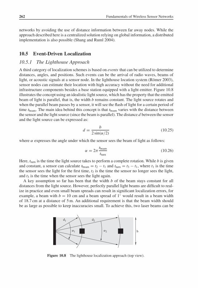
262 Fundamentals of Wireless Sensor Networks
networks by avoiding the use of distance information between far away nodes. While theapproach described here is a centralized solution relying on global information, a distributedimplementation is also possible (Shang and Ruml 2004).
10.5 Event-Driven Localization
10.5.1 The Lighthouse Approach
A third category of localization schemes is based on events that can be utilized to determinedistances, angles, and positions. Such events can be the arrival of radio waves, beams oflight, or acoustic signals at a sensor node. In the lighthouse location system (Romer 2003),sensor nodes can estimate their location with high accuracy without the need for additionalinfrastructure components besides a base station equipped with a light emitter. Figure 10.8illustrates the concept using an idealistic light source, which has the property that the emittedbeam of light is parallel, that is, the width b remains constant. The light source rotates andwhen the parallel beam passes by a sensor, it will see the flash of light for a certain period oftime tbeam. The main idea behind this concept is that tbeam varies with the distance betweenthe sensor and the light source (since the beam is parallel). The distance d between the sensorand the light source can be expressed as:
d = b
2 sin(α/2)(10.25)
where α expresses the angle under which the sensor sees the beam of light as follows:
α = 2πtbeam
tturn(10.26)
Here, tturn is the time the light source takes to perform a complete rotation. While b is givenand constant, a sensor can calculate tbeam = t2 − t1 and tturn = t3 − t1, where t1 is the timethe sensor sees the light for the first time, t2 is the time the sensor no longer sees the light,and t3 is the time when the sensor sees the light again.
A key assumption so far has been that the width b of the beam stays constant for alldistances from the light source. However, perfectly parallel light beams are difficult to real-ize in practice and even small beam spreads can result in significant localization errors, forexample, a beam with b = 10 cm and a beam spread of 1◦ would result in a beam widthof 18.7 cm at a distance of 5 m. An additional requirement is that the beam width shouldbe as large as possible to keep inaccuracies small. To achieve this, two laser beams can be
d1 d2
a1 a2 b
Figure 10.8 The lighthouse localization approach (top view).

Localization 263
used to create the outline of a “virtual” parallel beam (the sensor nodes are only interestedin detecting the edges of the virtual beam which are represented by the two laser beams).
10.5.2 Multi-Sequence Positioning
The Multi-Sequence Positioning (MSP) approach (Zhong and He 2007) works by extract-ing relative location information from multiple simple one-dimensional orderings of sen-sor nodes. For example, Figure 10.9 shows a small sensor network with five nodes withunknown locations and two anchor nodes. Events are generated by event generators at differ-ent locations one at a time (e.g., ultrasound propagations or laser scans with diverse angles).The nodes in the sensor field observe these events at different times, depending on theirdistances to the event generators. For each event, we can establish a node sequence, that is,a node ordering (including both the sensor and the anchor nodes) based on the sequentialdetection of the event. Then, a multisequence processing algorithm narrows the potentiallocations for each node to a small area and, finally, a distribution-based estimation methodestimates the exact locations.
The basic concept of the MSP algorithm is to split a sensor network area into small piecesby processing node sequences. For example, in Figure 10.9, performing a straight-line scanfrom top to bottom results in a node sequence 2, B, 1, 3, A, 4, 5. The basic MSP algorithmuses two straight lines to scan an area from different directions, treating each scan as anevent. In Figure 10.9, a left-to-right scan results in a node sequence 1, A, 2, 3, 5, B, 4. Sincethe anchor locations are known, the two anchors split the area into nine parts. This processcan be extended to cut the area into smaller pieces by increasing the number of anchors andscans (from different angles). The basic MSP algorithm processes each node sequence todetermine the boundaries of a node (by searching for the predecessor and successor anchornodes for the node) and shrinks the location area of this node according to the newly obtainedboundary information. Finally, a centroid estimation algorithm sets the center of gravity ofthe resulting polygon as the estimated location of the target node.
Event 1
Event 2 Event 4
Anchor
A
2
B
3
Event 3
Node Sequence for Event 21 – 2 – B – A – 3 – 5 – 4
Node Sequence for Event 34 – 5 – B – 3 – A – 2 – 1
Node Sequence for Event 4B – 2 – 3 – 1 – 4 – A – 5
Node Sequence for Event 1A – 1 – 5 – 3– 4 – 2 – B
5
Anchor
4
1
Figure 10.9 Basic concept of MSP.

264 Fundamentals of Wireless Sensor Networks
Exercises
10.1 Why is localization needed in wireless sensor networks? Name at least two concretescenarios or applications where localization is required.
10.2 A node’s position in two-dimensional space is (x, y) = (10, 20) with a maximumerror of 2 in the x direction for 95% of all measurements and a maximum error of 3in the y direction for 90% of all measurements. What is the accuracy and the precisionof this location information?
10.3 Explain the difference between physical and symbolic positions and name at leasttwo examples for each type.
10.4 Define the terms anchor-based localization and range-based localization.
10.5 Time of Arrival (ToA) is one example of a ranging technique. Answer the followingquestions (assume a propagation time of 300 m/s):
(a) What is the advantage of two-way ToA over one-way ToA?(b) In a synchronized network with unknown synchronization error, an anchor node
periodically broadcasts an acoustic signal to sensor nodes in its range. At time1000 ms on the anchor node’s clock, the anchor node issues a beacon, which isreceived by node A at time 2000 ms (on node A’s clock). What is the distancethat A can now compute?
(c) Instead of computing the distance itself, node A also responds with an acous-tic signal issued at time 2500 ms, which is received by the anchor node at time3300 ms. What is the distance computed by the anchor node? What can you sayabout the synchronization of anchor node and node A?
10.6 What is the main disadvantage for both TDoA and AoA ranging techniques?
10.7 RSS-based localization techniques are often combined with a process called RF pro-filing, that is, the mapping of the effects of objects in the environment on signalpropagation. Why is this necessary and can you think of examples of such objects?
10.8 Two nodes A and B are known to be positioned at locations (0, 0) (node A) and (1, 1)
(node B) in two-dimensional space. A third node C wishes to determine its posi-tion using trilateration. Based on ranging techniques, node C knows its distances tonode A (d(A,C) = √
0.75) and node B (d(B,C) = √0.75). What are the two possible
positions of C?
10.9 Three nodes A, B, and C are known to be positioned at locations (0, 0), (10, 0), and(4, 15), respectively. Node D is estimated to be a distance of 7 from A, a distanceof 7 from B, and a distance of 10.15 from C. Determine the location of D usingtrilateration.
10.10 Consider the two-dimensional topology in Figure 10.10. The sensor node in the centercan select three of the six anchor nodes as basis for trilateration. Which nodes shouldthe sensor node select? Justify your answer, that is, what guideline for anchor selec-tion should be considered? What would this guideline be in three-dimensional space?

Localization 265
B6
Beacon
Sensor
B1
B2
B3
B4
B5
Figure 10.10 Exercise 10.10.
10.11 Two nodes A and B do not know their own positions, but they can hear beacons intheir proximities. Node A can hear beacons located at (4, 2) and (2, 5). Node B canhear beacons located at (2, 5) and (3, 7). All nodes have a radio range of 2 units.
(a) Are either (3, 3.5) or (3, 4.5) possible locations for node A?(b) Are either (2, 6) or (4, 5) possible locations for node B?
10.12 What are the differences between iterative and collaborative multilateration?
10.13 Explain the concept of GPS localization and answer the following questions:
(a) Why are three satellites enough to obtain a position on the globe?(b) Why is it preferred to have at least four satellites available for localization?(c) What is the purpose of the monitor stations and the master control station?(d) Why is it typically not feasible to have all wireless sensor nodes equipped with
a GPS receiver?
10.14 Explain the difference between range-based and range-free localization.
10.15 Figure 10.11 shows a network topology with three anchor nodes. The distancesbetween anchors A1 and A2, anchors A1 and A3, and anchors A2 and A3 are 40 m,110 m, and 35 m, respectively. Use the Ad Hoc Positioning System to estimate thelocation of the gray sensor node (show each step of your process).
A2
A1
A3
Figure 10.11 Exercise 10.15.

266 Fundamentals of Wireless Sensor Networks
10.16 For the APIT test, can you show a concrete scenario where a node M would cometo the wrong conclusion that it must be inside a triangle? Use a scenario where nodeM has at least three neighbors. Can you also show an example where node M wouldcome to the wrong conclusion that it must be outside a triangle?
10.17 A sensor node in a WSN using the lighthouse approach for localization detects thefirst beam of light at time 0 s and the second beam of light at time 0.25 s. The nexttime the first beam of light is detected is 7 s. The distance of the two light sources(beam width) is 10 cm. What is the distance of the sensor to the light emitter?
ReferencesDana, P.H. (1997) Global Positioning System (GPS): Time-dissemination for real-time applications. Real-Time,
Systems 12 (1), 9–40.Gavish, M., and Weiss, A.J. (1992) Performance analysis of bearing-only target location algorithms. IEEE Trans-
actions on Aerospace and Electronic Systems 28 (3), 817–828.Gustafsson, F., and Gunnarsson, F. (2003) Positioning using time-difference of arrival measurements. Proc. of the
IEEE International Conference on Acoustics, Speech, and Signal Processing .He, T., Huang, C., Blum, B.M., Stankovic, J.A., and Abdelzaher, T. (2003) Range-free localization schemes for
large scale sensor networks. Proc. of the 9th Annual International Conference on Mobile Computing andNetworking (MobiCom).
Hightower, J., and Borriello, G. (2001) Location systems for ubiquitous computing. Computer 34 (8), 57–66.Hofmann-Wellenhof, B., Lichtenegger, H., and Collins, J. (2008) Global Positioning System: Theory and Practice
(5th edn). Springer.Lu, Y., Wang, W., Zhong, Y., and Bhargava, B. (2003) Study of distance vector routing protocols for mobile ad
hoc networks. Proc. of the 1st IEEE International Conference on Pervasive Computing and Communications(PerCom).
Mao, G., Fidan, B., and Anderson, B.D.O. (2007) Wireless sensor network localization techniques. ComputerNetworks: The International Journal of Computer and Telecommunications Networking 51 (10), 1389–1286.
Monteiro, L.S., Moore, T., and Hill, C. (2005) What is the accuracy of DGPS? The Journal of Navigation 58 (2),207–225.
Niculescu, D., and Nath, B. (2001) Ad hoc positioning system (APS). Proc. of the IEEE Global Telecommunica-tions Conference (GLOBECOM).
Peng, R., and Sichitiu, M.L. (2006) Angle of arrival localization for wireless sensor networks. Proc. of the 3rdAnnual IEEE Communications Society Conference on Sensor and Ad Hoc Communications and Networks .
Romer, K. (2003) The lighthouse location system for smart dust. Proc. of the 1st International Conference onMobile Systems, Applications and Services (pp. 15–30).
Savvides, A., Han, C.C., and Strivastava, M.B. (2001) Dynamic fine-grained localization in ad hoc networks ofsensors. Proc. of the 7th Annual International Conference on Mobile Computing and Networking .
Shang, Y., and Ruml, W. (2004) Improved MDS-based localization. Proc. of the 23rd Annual Joint Conferenceof the IEEE Computer and Communications Societies (INFOCOM).
Shang, Y., Ruml, W., Zhang, Y., and Fromherz, M. (2004) Localization from connectivity in sensor networks.IEEE Transactions on Parallel and Distributed Systems 15 (11), 961–974.
Siqueira, I.G., Ruiz, L.B., Loureiro, A.A.F., and Nogueira, J.M. (2007) Coverage area management for wirelesssensor networks. International Journal of Network Management 17 (1), 17–31.
Stansfield, R.G. (1947) Statistical theory of DF fixing. Journal of IEE 14, Pt. III A (15), 762–770.Stojmenovic, I. (2002) Position based routing in ad hoc networks. IEEE Communications Magazine 40 (7),
128–134.Tekdas, O., and Isler, V. (2007) Sensor placement algorithms for triangulation based localization. Proc. of the
IEEE International Conference on Robotics and Automation (pp. 4448–4453).Zhong, Z., and He, T. (2007) MSP: Multi-sequence positioning of wireless sensor nodes. Proc. of the 5th Inter-
national Conference on Embedded Networked Sensor Systems (pp. 15–28).

11SecuritySecurity and privacy are enormous challenges in all types of wired and wireless networks.These challenges are of even greater importance in wireless sensor networks, where theunique characteristics of these networks and the application purposes they serve make themattractive targets for intrusions and other attacks. In applications such as battlefield surveil-lance and assessment, target tracking, monitoring civil infrastructure such as bridges andtunnels, and assessment of disaster zones to guide emergency response activities, any breachof security, compromise of information, or disruption of correct application behavior canhave very serious consequences. Sensor networks are frequently used in remote areas, left tooperate unattended and therefore providing an easy target for physical attacks, unauthorizedaccess, and tampering. Sensor nodes are typically very resource-constrained and operate inharsh environments, which further facilitates compromises and makes it often difficult to dis-tinguish security breaches from node failures, varying link qualities, and other commonlyfound challenges in sensor networks. Finally, these resource constraints require securitymechanisms that are customized for WSN applications, such that the limited resources areused efficiently. This chapter provides an overview of the security concerns of WSNs andillustrates possible solutions to providing security and privacy protection. Note that the termsattacker , intruder , and adversary are used interchangeably to describe an entity (person ordevice) that performs an attack on a network or system.
11.1 Fundamentals of Network Security
Computer and network security is the collection of all policies, mechanisms, and servicesthat afford a computer system or network the required protection from unauthorized accessor unintended uses. Most security mechanisms are built to address three well-known ser-vices in the CIA security model: Confidentiality, Integrity , and Availability . The followingdescribes these services in more detail:
1. Confidentiality: Security mechanisms must ensure that only the intended receiver cancorrectly interpret a message and that unauthorized access and usage is prevented. Forexample, confidentiality ensures that sensitive information such as a person’s social secu-rity number or credit card information are not obtained by an unauthorized individual.
2. Integrity: Security mechanisms must ensure that a message cannot be modified as itpropagates from the sender to the receiver, that is, unauthorized individuals should notbe able to destroy or alter the contents of sensitive information.
Fundamentals of Wireless Sensor Networks: Theory and Practice Waltenegus Dargie and Christian Poellabauer 2010 John Wiley & Sons, Ltd

268 Fundamentals of Wireless Sensor Networks
3. Availability: Security mechanisms must ensure that a system or network and its applica-tions are able to perform their tasks at any time without interruption. Availability is oftenmeasured in terms of percentages of up or down time.
Figure 11.1 illustrates examples of attacks on a transmission between a sender and itsintended receiver. Eavesdropping refers to the reception of a message by an unauthorizedindividual, which can be prevented using confidentiality measures. A man-in-the-middleattack refers to a situation where an unauthorized individual or system positions itselfbetween the sender and receiver such that the sender’s messages are intercepted, modified,and retransmitted to the receiver (where the receiver believes the received message camedirectly from the original sender). This illustrates the need for integrity mechanisms.Finally, a denial-of-service attack refers to an adversary’s attempt to disrupt the transmis-sion or service provided by the sender. For example, the adversary can overload the senderwith requests and tasks such that the sender is not able to transmit its message (in a timelyfashion) to the receiver. This type of attack necessitates security mechanisms that ensureavailability.
In addition to the three components of the CIA triad, authentication refers to the processof establishing or confirming the identify of a user or a device, ensuring that a message camefrom who it claims to have come from. Also, nonrepudiation refers to the process of provingthat a person or device has performed a transaction or transmission. Digital signatures areoften used to support both authentication and nonrepudiation, but are also used to provideconfidence that a message has not been altered (i.e., integrity).
In all types of communication networks, there are several fundamental security mecha-nisms that can be used to provide confidentiality, integrity, and availability. Cryptographyis the process of hiding and protecting information using encoding and decoding mecha-nisms. In symmetric key cryptography , a single key between two communicating parties isused for the encryption and decryption of a message. For example, a simplistic encodingstrategy could be to replace each plaintext letter with another letter that is a certain numberof positions down the alphabet. For example, using a shift of 2 would replace the letter A
Man-in-the-Middle(Integrity)
SenderIntendedReceiver
Eavesdropping(Confidentiality)
Denial-of-Service(Availability)
Figure 11.1 Examples of attacks and the CIA model.

Security 269
with the letter C. In this shift cipher , the fixed shift value is then the symmetric key. A majorchallenge in the use of symmetric cryptographic techniques is the secure distribution of theshared key between the two communicating parties. Popular examples of symmetric keycryptographic mechanisms include DES, AES, and IDEA (Menezes et al. 1996).
In contrast to this approach, public key cryptography , such as the well-known RSA algo-rithm (Rivest et al. 1983) or the Diffie–Hellman key agreement protocol (Menezes et al.1996), rely on a pair of keys. A node generates both a secret key and a public key , where thesecret key will never be communicated with any other node. The public key, on the otherhand, can be shared freely with anyone in the network. Any message encrypted with thesecret key can only be deciphered using the corresponding public key (e.g., this can be usedto authenticate the identity of the sender). Any message encrypted with the public key canonly be deciphered using the corresponding secret key (e.g., this can be used to provideconfidentiality).
11.2 Challenges of Security in Wireless Sensor Networks
Security has been a challenge in computing systems and networks for several decades,during which the types of attacks and the security measures and mechanisms to counterthem have advanced and developed significantly, particularly because of the rapid growthof the Internet. Compared to the traditional attacks and security mechanisms developed forthe Internet, WSNs exhibit a variety of unique challenges that must be considered whenaddressing the security concerns that may arise in sensor network applications:
1. Resource constraints: Traditional security mechanisms that have high overheads are notsuitable for resource-constrained WSNs. Many security mechanisms are computation-ally expensive or require communication with other nodes or “remote” devices (e.g.,for authorization purposes), thereby leading to energy overheads. Small sensor devicesare also constrained in their available memory and storage capacities. Common sensordevices have very limited amounts of memory, for example, TelosB devices only have10 kbytes RAM and 48 kbytes flash memory available. Traditional security algorithmsthat require a significant amount of memory and storage space are therefore infeasiblefor such sensors.
2. Lack of central control: It is often infeasible to have a central point of control in sensornetworks, for example, because of their large scale, resource constraints, and networkdynamics (topology changes, network partitioning). Therefore, security solutions shouldbe decentralized and nodes must collaborate to achieve security.
3. Remote location: The first line of defense against security attacks is to provide onlycontrolled physical access to a sensor node. Many WSNs are left unattended, becausethey are operated in remote and hard-to-reach locations, deployed in environments opento public access, or so large that it would be infeasible to continuously monitor and protectsensor nodes from attacks. These challenges make it difficult to prevent unauthorizedphysical access and to detect tampering with the sensor devices, particularly since the lowcost of many sensor nodes may prohibit advanced (and expensive) protective measures.
4. Error-prone communication: Packets in WSNs may be lost or corrupted due to a varietyof reasons, including channel errors, routing failures, and collisions. This may interferewith some security mechanisms or their ability to obtain critical event reports. Further-more, this may make it difficult to distinguish “benign” erroneous communications ornode and link failures from malicious attacks.

270 Fundamentals of Wireless Sensor Networks
Certain characteristics of sensor networks, on the other hand, facilitate the provision ofsecurity. For example, the self-managing and self-repairing nature of a WSN may allow itto continue to operate even if a sensor or entire regions of the sensor network have beencompromised. Redundancy in a sensor network allows it to gather information about eventsin the environment even when some sensors are unavailable due to an attack. Furthermore,this redundancy can be used to detect, isolate, and mask potentially compromised nodes.
Data collected by sensors may contain sensitive information and should not be leaked tounauthorized devices. Further, encryption keys and information about sensors themselves(e.g., identity, location, etc.) must be protected to prevent eavesdropping and attacks basedon traffic analysis. These challenges require measures that provide data confidentiality forsensor networks. Integrity is required to prevent adversaries from modifying sensor data, forexample, with the purpose of injecting false readings and therefore affecting the responseto the sensor readings. Authentication is necessary to ensure that any data disseminated ina sensor network originates from the correct source, particularly when a single node con-trols the entire network (e.g., a base station establishing routes or distributing multicasttree information). Further, many security attacks in sensor networks have the goal to dis-rupt the correct functioning of the network altogether, necessitating measures that ensurenetwork availability. An additional requirement in sensor networks is the need for datafreshness , which ensures that sensor data are recent and no old recordings of such data arebeing replayed. This is particularly important for key distribution schemes, for example, anattacker could record shared keys that are being exchanged in a network and replay these keydistribution messages at a later time. Finally, many node and network management respon-sibilities found in WSNs provide adversaries with opportunities for attacks. For example,sensor node localization is important for correctly interpreting sensor data, for geographicrouting protocols, and for redundancy elimination. However, many localization techniquesrequire the exchange of information among sensors (e.g., beacons carrying positions, timestamps, and identity information) that may necessitate encryption. Similarly, time synchro-nization in sensor networks is based on message exchange among sensor nodes, where anadversary could inject false time stamps to increase synchronization errors among sensors.
11.3 Security Attacks in Sensor Networks
Sensor networks are vulnerable to a variety of attacks that attempt to compromise the net-work’s operation and the data the sensor nodes generate. Specifically when sensor networksserve application purposes such as battlefield assessments and monitoring of civil infrastruc-ture, they require protection from unauthorized access and tampering. This section describesa variety of security attacks that could occur in a WSN.
11.3.1 Denial-of-Service
A Denial-of-Service (DoS) attack can be characterized as an attempt of an adversary to stopa network from functioning or to disrupt the services a network provides. In wireless sensornetworks, DoS attacks can occur at various layers of the protocol stack, where some mayaffect multiple layers simultaneously or attempt to exploit interactions between them (Woodand Stankovic 2002).

Security 271
11.3.1.1 Physical Layer DoS
The wireless medium used in a WSN facilitates a variety of attacks. A jamming attack occurswhen an adversary interferes with the radio frequencies of a WSN. If well positioned, afew attacking nodes can disable an entire network, even if the number of attacking nodesis much smaller than the number of nodes in the network. Even a single attacking nodecould disable an entire network if it is positioned close to a “critical” node (e.g., a gateway,therefore preventing any sensor data from leaving the sensor network) or its transmissionpower is large such that all nodes in a network may be prevented from correctly receiv-ing any meaningful data. A common technique against jamming is to use spread-spectrumcommunication, as found in well-known standards such as IEEE 802.11 and Bluetooth.For example, in frequency-hopping spread spectrum (FHSS), communicating devices fre-quently hop between frequencies according to a certain hopping sequence. A jammer eithermust know this sequence to be able to jam the correct frequency for continuous disruption,or must jam a large frequency band. In addition, sensor networks should be able to detect andrespond to jamming attacks in the network, for example, by switching nodes into low-powersleep modes (in order to preserve energy), while awakening them periodically to check ifthe jamming attack is still active. Nodes may also want to alert a gateway or base stationto report the attack. Toward this end, nodes detecting a jamming attack could issue briefalerts to their neighbors and if at least one of these neighbors is outside the region of theattack (i.e., it is able to receive the alert message without interference), the message can bepropagated to other nodes including the base station.
A tampering attack in a sensor network occurs when an adversary obtains physical accessto a sensor node, allowing the attacker to destroy or modify the device, gain access to sen-sitive information (e.g., cryptographic keys), or use the device as an entry point for furtherattacks into the network. Possible strategies to protect a device from tampering and theconsequences thereof include using tamper-proof materials and enclosures and to disable adevice or delete its information when an attack is detected. For example, a technique oftenused in systems handling sensitive information (e.g., credit card payment terminals) is toerase all such data whenever a light sensor activates (e.g., due to the terminal’s enclosurebeing opened).
11.3.1.2 Link Layer DoS
A collision attack at the link layer (Wood and Stankovic 2002) attempts to interfere withpacket transmissions, thereby causing costly exponential backoff procedures and retrans-missions in some MAC protocols. While error-correcting codes can be used to recover fromcorrupted bits in a packet, they may not be able to recover from all types of interferences(e.g., if too many bits have been corrupted) and they incur additional resource and energyoverheads. An attacker could also attempt to cause collisions near the end of a frame, caus-ing a node to repeatedly retransmit the entire packet. The goal of an attacker could be tocause the premature depletion of the node’s energy resources (exhaustion attack). Similarly,a malicious node could exploit certain handshake techniques often found in MAC protocols.For example, an attacker could continuously issue an RTS message (IEEE 802.11 protocol)to prompt a CTS response from another node, eventually exhausting the energy resourcesof both nodes.

272 Fundamentals of Wireless Sensor Networks
11.3.2 Attacks on Routing
One example of an attack on routing protocols of sensor networks is the blackhole attack(Karlof and Wagner 2003). With this type of attack, an adversary attempts to be a forwarderof data for one or more routes across the network. A malicious node can then simply dropall traffic that should pass through this node, therefore, such traffic never reaches the desti-nation. A similar attack is called the selective forwarding attack (Karlof and Wagner 2003),where only packets that match certain criteria are dropped instead of dropping all packetsindiscriminately. Selective forwarding attacks are more difficult to detect or react upon thanblackhole attacks since they are harder to distinguish from packet losses due to mobility orchannel errors.
A rushing attack (Hu et al. 2003) on a sensor network exploits the nature of the route dis-covery procedure of on-demand routing protocols, for example, as found in protocols suchas AODV and DSR. In this type of attack, a malicious node immediately forwards incomingroute request messages to its neighbors, therefore “rushing” these messages without consid-eration of any protocol rules (e.g., that specify certain timeout or queuing procedures beforeforwarding). As a consequence, the node has an increased probability of being part of thechosen route between source and destination.
A sinkhole attack (Karlof and Wagner 2003) is another variant of the blackhole attack.However, to attract as much traffic as possible, the malicious node attempts to position itselfon the path of as many network flows as possible. Traffic is therefore drawn toward thissinkhole, providing an attacker with an opportunity to disrupt or tamper with as much trafficas possible.
A Sybil attack occurs when an attacker claims to have several identities in the network.Similarly, in location-based routing protocols, an attacker claims to be at several locationssimultaneously. If many nodes believe that this malicious node is their neighbor, there is agood chance that they will choose this node as forwarding node for their network traffic.
Another attack on the routing procedure of a sensor network is the wormhole attack . Thisattack is performed by nodes that have more resources available than typical sensor nodesin the network. For example, two collaborating attackers may attempt to deceive the restof the network by possessing an out-of-band (and often bandwidth-rich) communicationchannel between themselves. To the rest of the network, this appears to be a fast, high-bandwidth link, which is desirable for many routing techniques. With this approach, theattacker nodes can fake an efficient and short path to the gateway of a network, thereforeattracting a significant amount of traffic and enabling a variety of other attacks, such as theblackhole or sinkhole attacks.
11.3.3 Attacks on Transport Layer
The transport layer of the network protocol stack is responsible for managing end-to-endconnections, for example, two well-known transport layer protocols are TransmissionControl Protocol (TCP) for reliable stream-based communication and User DatagramProtocol (UDP) for unreliable packet-based communication. The flooding attack (Woodand Stankovic 2002) exploits the fact that many transport protocols (such as TCP) maintainstate information and are therefore vulnerable to memory exhaustion. For example, anattacker may repeatedly make new connection requests, each adding more state informationat the affected node and potentially leading to the node refusing further connections due

Security 273
to resource exhaustion. This in turn prevents connection requests from legitimate nodesfrom succeeding.
In the desynchronization attack, an adversary attempts to disrupt the communicationbetween two legitimate nodes by repeatedly forging messages to these nodes. For example,reliable transport-layer protocols may use sequence numbers to keep track of successfullyreceived packets, identify packet loss, and detect duplicates. Fake packets issued by anadversary can use these sequence numbers to make a node believe that its packets havenot arrived at the destination, thereby eliciting resource-costly retransmissions.
11.3.4 Attacks on Data Aggregation
Data aggregation and data fusion are often used to combine multiple sensor data and to elim-inate redundant information. Aggregation can often have beneficial effects on the resourcerequirements of sensor flows, for example, by reducing the frequency of transmissions orthe packet sizes. Even simple aggregation functions can easily be influenced by an attackersuch that a network’s behavior can be altered (Wagner 2004). For example, the averagefunction f (x1, . . . , xn) = (x1 + · · · + xn)/n is insecure even in the presence of a singlemalicious node. By replacing one real measurement x1 with a fake reading x∗
1 , the average ischanged from y = f (x1, ..., xn) to y∗ = f (x∗
1 , x2, ..., xn) = y + (x∗1 − x1)/n. An attacker
can freely choose the value of x∗1 and, therefore, can control the outcome of the aggregation.
Similarly, the sum , minimum , and maximum functions are also insecure. The sumf (x1, ..., xn) = x1 + · · · + xn can be modified at will by maliciously replacing a real mea-surement x1 with a fake reading x∗
1 . The minimum function f (x1, ..., xn) = min(x1, ..., xn)
is also insecure, even though replacing a real measurement with a fake value does notalways affect the function’s outcome. That is, replacing x1 with x∗
1 only raises the minimumif x1 is the unique smallest sensor reading among all xi . However, an attacker can modifythe computed minimum by choosing x∗
1 to be very small compared to all correct readings.By symmetry, the maximum function is also insecure, since an attacker can raise themaximum value by hijacking a single sensor reading.
In contrast, the effect of hijacking a single sensor reading may be comparably small for thecount operation if the number of correct readings is sufficiently large. The count functionis similar to the sum function, except that each sensor reading only contributes 0 or 1 tothe result of the operation. That is, an attacker with control over k compromised nodes canchange the outcome of the function by at most k, which may be negligible if k is smallcompared to the total number of sensor inputs.
11.3.5 Privacy Attacks
While the security threats described so far are mainly targeted at disrupting a network fromcorrect operation, the vast amount of information collected in a WSN itself is also at riskof potential abuse. That is, an adversary may attempt to obtain sensitive information byaccessing information stored on a sensor node or by eavesdropping on the network (Gruteseret al. 2003). The broadcast nature of wireless networks makes it easy to monitor and capturethe transmissions between nodes, particularly when no cryptographic mechanisms are usedto protect the sensor data. Eavesdropping can also be combined with traffic analysis (Denget al. 2005a), which can be used by an adversary to identify sensor nodes of interest in a
274 Fundamentals of Wireless Sensor Networks
network. For example, increases in communications between certain nodes can indicate anincreased level of activity (and therefore the presence of data that could be compromised) inthose parts of the network. Similarly, traffic analysis can be used to identify nodes that maybe more important to network operation than others, such as base stations and gateways.
11.4 Protocols and Mechanisms for Security
In order to defend against the many possible attacks in a WSN, a variety of security protocolsand other defense mechanisms can be used. This section presents and discusses a varietyof such protocols and mechanisms with a particular focus on their applicability in sensornetworks.
11.4.1 Symmetric and Public Key Cryptography
While public key cryptography can be used to provide confidentiality, integrity, and authen-tication, public key algorithms are computationally very expensive, which may limit theiruse in resource-constrained sensor networks (Gaubatz et al. 2004). Symmetric key cryptog-raphy approaches can be significantly more resource-efficient, which makes them the morecommon choice in WSNs, even though implementations of RSA (Rivest et al. 1983) andECC (elliptic curve cryptography) (Menezes et al. 1996) for resource-constrained sensorsdo exist. A major disadvantage of symmetric key approaches is the problem of key distri-bution, that is, the shared symmetric key must first be known to both communicating nodesbefore they can exchange data securely.
11.4.2 Key Management
Symmetric cryptographic schemes are the common choice for sensor networks whenresource constraints prohibit the use of the more complex public key schemes. However, amajor shortcoming of symmetric cryptography is the need for key management, that is, thereliable and secure establishment of shared cryptographic keys among neighboring nodesin a WSN. For example, the Peer Intermediaries for Key Establishment (PIKE) approach(Chan and Perrig 2005) is a technique that uses sensor nodes as trusted intermediaries forthe distribution of keys. In this approach, every sensor shares a different pairwise key witheach of O(
√n) other nodes, where n is the number of nodes in the network. Furthermore,
the keys are deployed such that for any pair of nodes A and B, there exists at least one node,C, that shares a pairwise key with both A and B. Each sensor in PIKE has an ID of the form(x, y), where x, y ∈ {0, 1, 2, ...,
√n − 1}. That is, the sensor network is represented as a
matrix with√
n rows and columns, where a node’s position in the matrix is the node’s ID.Then, each node (x, y) shares a pairwise key with each node in the two following sets:
(i, y) ∀i ∈ {0, 1, 2, ...,√
n − 1} (11.1)
(x, j) ∀j ∈ {0, 1, 2, ...,√
n − 1} (11.2)
For example, node (x, y) will share a key K(x,y),(1,y) with node (1, y) and another keyK(x,y),(2,y) with node (2, y). Altogether, a node will maintain 2(
√n − 1) keys. Figure 11.2

Security 275
shows a sample virtual ID space for 100 nodes, where each number represents the ID of anode (note that this representation does not reflect the actual physical positions of the sensornodes). The dark shaded boxes identify all nodes that share a key with node 91, while thelight shaded boxes indicate all nodes that share a key with node 14. Due to this approach,any two nodes in the network will be able to find two node IDs which will share pairwisekeys with both of them. Specifically, if node A has ID (xA, yA) and node B has ID (xB, yB),then the nodes with IDs (xA, yB) and (xB, yA) will share pairwise keys with both A and B. Ifnode A (e.g., node 14 in Figure 11.2) wants to perform key establishment with another node(e.g., node 91), A can identify the identities of potential intermediaries by looking for theintersections of the shaded boxes. For example, node 94 is in the same row as 91 and in thesame column as 14, therefore it shares keys with both of them and can serve as intermediary.Node 14 then encrypts the new key to be shared with node 91 using the existing key sharedwith node 94 and then sends the encrypted key to node 94. Node 94 decrypts the message,encrypts it again with the key shared with node 91 and sends the new message to node 91.Node 91 decrypts the message, obtains the new key, and confirms the receipt of the new keyby replying to node 14.
11.4.3 Defenses Against DoS Attacks
Denial-of-service (DoS) attacks in sensor networks are common and require effective mea-sures to avoid them or prevent them from spreading throughout the network. For example,when a jamming attack is detected or suspected, a sensor network can attempt to isolatethe affected region by routing traffic around the disabled parts of the network. Anothertechnique to limit the damage from jamming attacks is to use spread-spectrum techniquesas described in Section 11.3.1. At the link layer, collision and exhaustion attacks can beaddressed using error-correcting codes (which add processing and communication over-heads) and rate-limiting schemes that allow a device to ignore requests that could lead topremature energy depletion. Spoofing and alteration can be addressed at the network layerby using message authentication code or MAC (not to be confused with medium accesscontrol ), which can be viewed as the cryptographically secure checksum of a message.These checksums allow a receiver to verify whether a message has been spoofed or altered(Sen 2009).
20 21 22 23 24 25 ... 29
30 31 31 33 34 35 ... 39
. . . . . . .
. . . . . . .
. . . . . . .
90 91 92 93 94 95 ... 99
00 01 02 03 04 05 ... 09
10 11 12 13 14 15 ... 19
Figure 11.2 Virtual ID space in PIKE.

276 Fundamentals of Wireless Sensor Networks
The path-based denial-of-service attack (PDoS) is an attack in which the attacker over-whelms the nodes in a remote sensor network by flooding a multi-hop end-to-end communi-cation path with either replayed packets or randomly injected packets (Deng et al. 2005b).One-way hash chains are sequences of numbers where it is trivial to compute y = F(x),but computationally infeasible to compute x = F−1(y). Each node in the network utilizesthe hash chain to validate a received packet, that is, a node systematically cycles throughthe chain to determine whether the packet is from a trusted source. If a packet cannot bevalidated, it is dropped.
11.4.4 Defenses Against Aggregation Attacks
As previously discussed, many simple aggregation functions such as sum, minimum, andmaximum are inherently insecure. However, several techniques for improving the resilienceof aggregation functions can be used, for example, two such techniques are delayed aggre-gation and delayed authentication (Hu and Evans 2003).
In these techniques, it is assumed that the base station generates a one-way key chainusing a public one-way function F , where Ki = F(Ki+1). Each device stores key K0 beforedeployment where K0 = Fn(K) (i.e., F applied to a secret key n times). Then, the firstbase station transmissions will be encrypted using key K1 = Fn−1(K). Once all messagestransmitted using K1 have been received, the base station reveals K1. As a consequence, allnodes can compute F(K1) = F(Fn−1(K)) and verify that it matches K0 = Fn(K). Further,sensor nodes can then decrypt the messages that were previously transmitted encrypted withK0. In a similar manner, successive keys can be revealed until Kn = K is reached (if morekeys are needed, the base station can then start a new sequence).
Assume that four sensor nodes A–D are sending messages to the base station in anetwork structured as a tree as shown in Figure 11.3. Each node’s message contains the
IDG|Aggr(RA, RB, RC, RD)|MIC(KGi, Aggr(RA, RB, RC, RD)| ... (same from right side)|MIC(KHi, Aggr(RA, RB, RC, RD... readings from right side))
IDB|RB|MIC(KBi, RB)IDA|RA|MIC(KAi, RA)
IDC|RC|MIC(KCi, RC)|IDD|RD|MIC(KDi, RD)|MIC(KFi, Aggr(RC, RD))
IDA|RA|MIC(KAi, RA)|IDB|RB|MIC(KBi, RB)|MIC(KEi, Aggr(RA, RB))
IDE|Aggr(RA, RB)|MIC(KEi, Aggr(RA, RB)|IDF|Aggr(RC, RD)|MIC(KFi, Aggr(RC, RD)|MIC(KGi, Aggr(RA, RB, RC, RD))
similar tree onright side (not shown)
A D
E
G
H
Base Station S
B C
F
Figure 11.3 Secure aggregation example.

Security 277
sender’s ID, the sensor data, and a MAC calculated over the data using a temporary key.The parent node of the sensor node is not yet able to verify the MAC since the child’skey has not been revealed to the parent. The parent node (e.g., node E in Figure 11.3)stores this message and retransmits it to its own parent after a certain timeout value.E’s message to its parent G contains the messages received from its children (e.g., nodesA and B) and a MAC computed over the aggregate of A’s and B’s data using E’s key.This process continues, that is, every intermediate node combines the data coming from itschildren and adds its own MAC over the aggregate of all data using its own key. Once thebase station receives messages from its children, it can compute the final aggregate value.
The base station has a shared temporary key with each sensor node, therefore it can verifywhether a received message was transmitted by H by calculating the MAC of the aggregationusing KHi and comparing it to the MAC in the message. While this validates that H sent thefinal message, it does not validate that the message correctly reflects the readings from theother nodes. To validate data, the base station reveals temporary node keys to the networkby sending each key (along with a MAC) to all sensor nodes using its own current key Ki .After sending out all the node keys, the base station sends out its current key Ki such thatnodes are able to check the transmitted MAC values and to advance to the next key in thechain for future messages.
In summary, the described process delays both aggregation and authentication, forexample, aggregation does not take place at the first hop that would be able to perform thisaggregation, but at the second hop. While this may increase resource expenditures, it mayalso enable integrity guarantees where consecutive nodes have not been compromised.
11.4.5 Defenses Against Routing Attacks
Most attacks from the “outside” of a network can be prevented using simple link-layerencryption and authentication using a globally shared key (Karlof and Wagner 2003).Because the adversary is prevented from joining the network, attacks such as selectiveforwarding or sinkholes are not possible. However, when networks are attacked from the“inside”, for example, using a compromised node, this approach is ineffective and moresophisticated solutions are needed.
Sybil attacks can be addressed by verifying the identities of sensor nodes. For example,each sensor node could share a unique symmetric key with a trusted base station, which canbe used to verify each other’s identity. A base station can also limit the number of neighbors anode is allowed to have, that is, even when a node is compromised, it can only communicatewith its verified neighbors.
Sinkholes are difficult to defend against in protocols where routes are established on thebasis of information that is hard to verify, for example, reliability or energy measurements.Routes based on minimum hop counts are easier to verify, but the hop count can be mis-represented through a wormhole (Karlof and Wagner 2003). One category of protocols thatis resistant to these attacks is geographic routing, because networks using location-basedrouting techniques establish a topology on demand based on localized interactions andinformation, without the initiation from a base station. Since traffic is “naturally” routedtoward the physical location of the base station, it is difficult to redirect traffic elsewhere tocreate a sinkhole.

278 Fundamentals of Wireless Sensor Networks
In a rushing attack, a node’s goal is to exploit the route discovery process in on-demandrouting protocols to position itself on as many routes as possible. However, to prevent suchattacks, a combination of several protective measures can be used. For example, some attack-ers may forward route requests beyond the normal radio transmission range (e.g., using hightransmission power), thereby suppressing subsequent request messages from this route dis-covery. A secure neighbor detection approach (Hu et al. 2003) can be used to allow both thesender and the receiver of a route request to verify that the other party is in fact within thenormal transmission range. For example, a three-round mutual authentication protocol withtight delay timing can be deployed. In the first round, a node sends a neighbor solicitationpacket (either via broadcast or via unicast to a specific node). In the second round, a nodereceiving the solicitation packet responds with a neighbor reply message and in the thirdround, the initiator of this handshake communication sends a neighbor verification message,which includes broadcast authentication of a timestamp and the link from the source to thedestination.
11.4.6 Security Protocols for Sensor Networks
The Security Protocols for Sensor Networks (SPINS) project makes two main contributionsto defending against attacks: the Secure Network Encryption Protocol (SNEP) and a “micro”version of the Timed, Efficient, Streaming, Loss-tolerant Authentication (µTESLA) proto-col (Perrig et al. 2002). The main goal of the SNEP protocol is to provide confidentiality,two-party data authentication, and data freshness, while µTESLA provides authenticationfor data broadcast. Each node is assumed to have a secret key shared with the base station.
11.4.6.1 Secure Network Encryption Protocol
SNEP takes the resource limitations of typical sensor nodes into consideration by relyingon simple algorithms for encryption, authentication, and random number generation. Thekey properties of SNEP are its symmetric security, replay protection, and low communi-cation overhead. Symmetric security refers to the fact that the same message is encrypteddifferently each time. To achieve two-party authentication and integrity, SNEP uses a MAC,where the larger the MAC the more difficult it is for an adversary to guess the appropriatecode for a message. On the other hand, large codes also mean larger packet sizes.
Two communicating nodes A and B share a secret master key , which is used to derive fourindependent keys using a pseudorandom function. Two of these keys are used for encryptionof messages in each direction (KAB and KBA) and two keys are used as message integritycodes, again one for each direction (K ′
AB and K ′BA). A complete encrypted message has then
the following format:
A → B : {D}〈KAB,CA〉, MAC(K ′ABCA||{D}〈KAB,CA〉) (11.3)
where D is the data encrypted with the encryption key K and the counter is C. The MAC iscomputed in the form M = MAC(K ′, C||E). SNEP provides data authentication (using theMAC), replay protection (using the counter value in the MAC), freshness (the counter val-ues enforce a message ordering), semantic security (since the counter is encrypted with eachmessage, the same message will be encrypted differently each time), and low communica-tion overhead (assuming that the counter state is kept at each end point and is not sent in the

Security 279
message). Data freshness under SNEP is considered to be weak only since SNEP enforcesa sending order within a node B, but no absolute assurance to node A that a message wascreated by B in response to an event in A. In order to achieve strong freshness, a nonce (i.e.,a random number so long that an exhaustive search for all possible nonces is infeasible) canbe included in the protocol. Node A randomly generates nonce NA and sends it along witha request message to node B. Node B then returns the nonce with the response message inan authenticated protocol that operates as follows:
A → B : NA, RA (11.4)
B → A : {RB}〈KBA,CB〉, MAC(K ′BA, NA||CB||{RB}〈KBA,CB〉) (11.5)
If the MAC verifies correctly, A knows that node B generated its response after A’s request.The µTESLA protocol focuses on the need for authenticated broadcast in wireless sensor
networks. It relies on the symmetric mechanisms provided by SNEP to authenticate the firstpacket in a broadcast message. It is an extension of TESLA (Perrig et al. 2000), which wasnot designed for use in environments with limited computing resources. TESLA uses digitalsignatures to authenticate the initial packet and has an overhead of 24 bytes per packet, whichcan be significant for sensor networks, where messages are typically very small. Authenti-cated broadcast requires an asymmetric mechanism (otherwise any compromised receivercould forge messages from the sender), but asymmetric cryptographic mechanisms are oftenhigh in resource requirements. Instead, µTESLA emulates asymmetry through a delayeddisclosure of symmetric keys. µTESLA assumes that the base station and the sensor nodesare loosely time synchronized and each node knows an upper bound on the maximum syn-chronization error. When the base station sends a message, it authenticates it by computing aMAC on the packet with a key that is secret at this point. When a node receives the packet andthe key is unknown, the node knows that the MAC key is known only to the base station. Thenode stores the packet until the base station, at the time of key disclosure, broadcasts the ver-ification key to all receivers. The node can now use the key to authenticate the stored packet.
11.4.7 TinySec
The TinySec architecture is a lightweight and generic link-layer security package that devel-opers can easily integrate into sensor network applications (Karlof et al. 2004). It supportstwo different security options: (1) authenticated encryption (TinySec-AE), where data pay-load is encrypted and a MAC is used to authenticate a packet, and (2) authentication only(TinySec-Auth), where an entire packet is authenticated with a MAC (but the payload isleft unencrypted). TinySec relies on cipher block chaining (CBC) and a specially formatted8-byte initialization vector (IV) for encryption. For authentication, TinySec relies on effi-cient and fast cipher block chaining construction (CBC-MAC) for computing and verifyingMACs. An advantage of CBC-MAC is that since it relies on a block cipher, it minimizesthe number of cryptographic primitives that must be implemented, which is beneficial forsensor nodes with limited storage capacities. The length of the MAC is chosen to be only4 bytes, that is, an adversary can repeatedly attempt blind forgeries, which would lead tosuccess after at most 232 attempts. While this number appears small, it must be noted thatan adversary must assess the validity of a code by sending it to an authorized receiver. That

280 Fundamentals of Wireless Sensor Networks
further means that up to 232 messages must be transmitted, which provides a sufficient levelof security for sensor networks (Boyle and Newe 2008).
11.4.8 Localized Encryption and Authentication Protocol
The Localized Encryption and Authentication Protocol (LEAP) (Zhu et al. 2003) is a keymanagement protocol for sensor networks, designed to support in-network processing. Akey motivation for this protocol is the observation that different types of messages (e.g., con-trol packets versus data packets) in a sensor network have different security requirements.A single keying mechanism may not suitable for meeting these different requirements, forexample, while authentication may be needed for all types of packets, confidentiality mayonly be required for certain types of messages (e.g., aggregated sensor readings).
LEAP provides four keying mechanisms: individual keys , group keys , cluster keys , andpairwise shared keys . In the individual key mechanism, every node has its own unique keyshared with the base station. This key is used for confidential communication or for com-puting message authentication codes if a node wants the base station to verify its sensedreadings. A group key is a globally shared key that is used by the base station for the trans-mission of encrypted messages to the entire sensor network. Common examples of suchmessages include queries or interests. A cluster key is a key shared between a sensor nodeand its neighbors and is used for securing local broadcast messages (e.g., routing controlmessages). Finally, a pairwise shared key is a key shared by a sensor node and one of itsimmediate neighbors. LEAP uses these keys for secure communications among a pair ofnodes, for example, allowing a node to securely distribute its cluster key to its neighbors orto securely transmit its sensor readings to an aggregation node.
LEAP also provides a technique for local broadcast authentication. Toward this end, everynode generates a one-way key chain of certain length and transmits the first key in the chainto each neighbor, encrypted with the pairwise shared key. Whenever a node sends a message,it takes the next key from the chain (each key is called an AUTH key) and attaches it to themessage. These keys are disclosed in the reverse order of their generation and a receiver canverify the message based on the first received key or a recently disclosed AUTH key.
11.5 IEEE 802.15.4 and ZigBee Security
The IEEE 802.15.4 standard and the ZigBee specification are popular protocol choices forWSNs. Therefore, this chapter concludes with a discussion of the security measures avail-able in these protocols.
The IEEE 802.15.4 standard provides four basic security models: access control, mes-sage integrity, message confidentiality , and replay protection (Sastry and Wagner 2004).Security in IEEE 802.15.4 is handled by the MAC layer and an application can choose spe-cific security requirements by setting appropriate parameters in the radio stack (by default,security is not enabled). The standard distinguishes between eight security suites (outlinedin Table 11.1), each with different levels of protection for the transmitted data. The firstsuite offers no security, the second suite offers encryption only (AES – CTR), followed bya group of suites with authentication only (AES – CBC – MAC), and a group of suites withboth authentication and encryption (AES – CCM). Suites that offer authentication differ inthe sizes of the MAC, which varies from 32 to 128 bits. For every suite that offers encryption,

Security 281
Table 11.1 Security suites supported in IEEE 802.15.4(Sastry and Wagner 2004)
Name Description
Null No securityAES – CTR Encryption only, CTR modeAES – CBC – MAC – 128 128-bit MACAES – CBC – MAC – 64 64-bit MACAES – CBC – MAC – 32 32-bit MACAES – CCM – 128 Encryption and 128-bit MACAES – CCM – 64 Encryption and 64-bit MACAES – CCM – 32 Encryption and 32-bit MAC
IEEE 802.15.4 also offers optional replay protection consisting of monotonically increasingsequence numbers for messages to allow a recipient to detect replay attacks.
The first suite Null does not provide any security. All other security suites use theAdvanced Encryption Standard (AES) block cipher, which is also known as Rijndael. TheNational Institute of Standards and Technology defines five modes of operation, includingthe counter (CTR) and cipher block chaining (CBC) modes (Sastry and Wagner 2004).When authentication is needed, one of the three AES – CBC – MAC variants can be used,which compute a message integrity code using a block cipher in CBC mode. The threeAES – CCM suites combine encryption and authentication by using the counter mode andthe CBC mode (CCM is short for Counter with CBC – MAC).
In addition to the security features of IEEE 802.15.4, the ZigBee specification also intro-duces the concept of a trust center , a responsibility typically assumed by the ZigBee coordi-nator. The trust center is responsible for authentication of devices wishing to join a network(trust manager), maintaining and distributing keys (network manager), and enabling end-to-end security between devices (configuration manager).
ZigBee also differentiates between a residential and a commercial mode (Boyle andNewe 2008). In the residential mode, the trust center allows nodes to join the network, but itdoes not establish keys with the network devices. In the commercial mode, it generates andmaintains keys and freshness counters with every device in the network. The disadvantageof the commercial mode is its memory cost, which grows with the size of the network.
The ZigBee specification uses the CCM* mode for its security services, which is also acombination of CTR mode and CBC – MAC mode. Compared to the CCM mode, CCM*offers encryption-only and integrity-only capabilities. Similar to the specifications in theIEEE 802.15.4 standard, ZigBee has several levels of security, including no security, encryp-tion only, authenticated only, and both encryption and authentication. Levels that provideauthentication use a MAC that can vary from 4 to 16 bytes.
11.6 Summary
Like every other computer network, wireless sensor networks are exposed to a varietyof threats and attacks and like most other networks, sensor networks require supportfor confidentiality, integrity, and authentication to protect sensor nodes and sensor data.

282 Fundamentals of Wireless Sensor Networks
However, several unique characteristics of WSNs, such as remote deployment (whichfacilitates an adversary’s physical access to sensor nodes) and resource constraints, make iteasier to compromise sensors and sensor data. Further, many sensor networks are attractivetargets for attackers due to the nature of many WSN applications and the sensitive datathey generate (e.g., military applications, emergency response, health care). This chapterprovided a brief overview of several types of attacks commonly found in sensor networksand techniques and protocols to defend a network or to detect an intrusion or compromisednode. As WSNs continue to become more commonplace, it is to expect that securitychallenges will increase, the types and number of threats will evolve, and new solutions toprotect sensor networks and sensor data will be required.
Exercises
11.1 Describe the CIA security model. Which service(s) described in this model do youthink are essential for the following scenarios? Justify your answers.
(a) A WSN that allows emergency response teams to avoid risky and dangerous areasand activities.
(b) A WSN that collects biometric information collected at an airport.(c) A WSN that measures air pollution in a city for a research study.(d) A WSN that alerts a city of an impending earthquake.
11.2 What is a man-in-the-middle attack? Can you imagine a concrete WSN scenariowhere such an attack could be catastrophic?
11.3 Explain the concepts of symmetric and asymmetric keys. This chapter mentioneda shift cipher as a simple example of a cryptographic technique. Is this cipher asymmetric or an asymmetric key cryptography technique? What are the problemswith such a simple cipher?
11.4 Why do you think authentication can be a particularly significant problem in a WSN?
11.5 Explain some of the characteristics of a WSN that make routing security difficult toimplement.
11.6 While “typical” computers are in homes, offices, labs, etc., wireless sensor nodes areoften placed in places that are publicly open and accessible. What kind of attackscould an adversary initiate by accessing a single sensor node in a large-scale WSN?
11.7 What is “data freshness” and why is it important in sensor networks?
11.8 What is a denial-of-service attack? Explain the following attacks:
(a) Jamming attack(b) Exhaustion attack(c) Tampering attack
11.9 Consider routing attacks such as selective forwarding, sinkhole, blackhole, Sybil,rushing, and wormhole attacks. Describe briefly each type of attack and discuss howthese attacks could take place in the following types of networks:

Security 283
(a) A network using a table-based routing protocol such as OLSR.(b) A network using an on-demand routing protocol such as DSR.(c) A network using a location-based routing protocol such as GEAR.
11.10 In this chapter, data aggregation functions such as average, sum , and minimum werecalled “insecure”. What does this mean and which technique can be used to increasethe resilience of aggregation functions?
11.11 Consider the virtual ID space for the PIKE scheme in Figure 11.2. In this example,how many options does node 3 have to establish a key with node 15? Describe eachoption.
11.12 What is a “nonce”? How does SPINS use them and what services are provided bythe SNEP protocol?
11.13 What are the security models provided by IEEE 802.15.4? What is the purpose of thetrust center in ZigBee?
ReferencesBoyle, D., and Newe, T. (2008) Securing wireless sensor networks: Security architectures. Journal of Networks 3
(1), 65–77.Chan, H., and Perrig, A. (2005) PIKE: Peer intermediaries for key establishment in sensor networks. Proc. of the
24th Annual Joint Conference of the IEEE Computer and Communications Societies (INFOCOM), Miami,FL.
Deng, J., Han, R., and Mishra, S. (2005a) Countermeasures against traffic analysis attacks in wireless sensornetworks. Proc. of the IEEE Conference on Security and Privacy for Emerging Areas in CommunicationNetworks (SecureComm), Athens, Greece.
Deng, J., Han, R., and Mishra, S. (2005b) Defending against path-based DoS attacks in wireless sensor networks.Proc. of the 3rd ACM Workshop on Security of Ad Hoc and Sensor Networks (SANS), Alexandria, VA.
Gaubatz, G., Kaps, J.P., and Sunar, B. (2004) Public key cryptography in sensor networks revisited. Proc. of the1st European Workshop on Security in Ad Hoc and Sensor Networks, Heidelberg, Germany .
Gruteser, M., Schelle, G., Jain, A., Han, R., and Grunwald, D. (2003) Privacy aware location sensor networks.Proc. of the 9th USENIX Workshop on Hot Topics in Operating Systems (HotOS IX), Lihue, HI .
Hu, L., and Evans, D. (2003) Secure aggregation for wireless networks. Proc. of the Workshop on Security andAssurance in Ad Hoc Networks, Orlando, FL.
Hu, Y.C., Perrig, A., and Johnson, D. B. (2003) Rushing attacks and defense in wireless ad hoc network routingprotocols. Proc. of the 2nd ACM Workshop on Wireless Security, San Diego, CA.
Karlof, C., and Wagner, D. (2003) Secure routing in wireless sensor networks: Attacks and countermeasures. AdHoc Networks 1 (23), 293–315.
Karlof, C., Sastry, N., and Wagner, D. (2004) TinySec: A link layer security architecture for wireless sensornetworks. Proc. of the 2nd International Conference on Embedded Networked Sensor Systems, Baltimore,MD .
Menezes, A.J., Vanstone, S.A., and Oorschot, P.C.V. (1996) Handbook of Applied Cryptography . CRC Press,Boca Raton, FL.
Perrig, A., Canetti, R., Tygar, J., and Song, D. (2000) Efficient authentication and signing of multicast streamsover lossy channels. Proc. of the IEEE Symposium on Security and Privacy, Berkeley, CA.
Perrig, A., Szewczyk, R., Tygar, J.D., Wen, V., and Culler, D.E. (2002) SPINS: Security protocols for sensornetworks. Wireless Networks 8, 521–534.
Rivest, R.L., Shamir, A., and Adleman, L. (1983) A method for obtaining digital signatures and public key cryp-tosystems. Communications of the ACM 26 (1), 96–99.

284 Fundamentals of Wireless Sensor Networks
Sastry, N., and Wagner, D. (2004) Security considerations for IEEE 802.15.4 networks. Proc. of the 3rd ACMWorkshop on Wireless Security, Philadelphia, PA.
Sen, J. (2009) A survey on wireless sensor network security. International Journal on Communications Networksand Information Security (IJCNIS) 1 (2), 59–82.
Wagner, D. (2004) Resilient aggregation in sensor networks. Proc. of the 2nd ACM Workshop on Security of AdHoc and Sensor Networks, Washington, DC .
Wood, A.D., and Stankovic, J.A. (2002) Denial of service in sensor networks. Computer 35 (10), 54–62.Zhu, S., Setia, S., and Jajodia, S. (2003) LEAP: Efficient security mechanism for large-scale distributed sensor
networks. Proc. of the 10th ACM Conference on Computer and Communications Security, Washington, DC .

12Sensor Network ProgrammingApplication development for sensor networks differs in many ways from programming“traditional” distributed computing systems. Examples of such differences include the con-tinuous interaction of sensor nodes with their physical environment, the stringent resourceconstraints of sensor nodes, the ad hoc deployment of many sensor networks, and the fre-quent changes in network topology due to failures or mobility. This chapter discusses aspectsof programming large sensor networks that consider these challenges. From the networkdeveloper’s perspective, the goal is to design and program a reliable and efficient wirelesssensor network that can cope with the dynamics and uncertainties present in sensing sys-tems. From the user’s perspective, the network is often viewed as a database and the usersinteract with sensor nodes via queries, which must be responded to in a reliable and efficientfashion. Many simulation tools and techniques are closely tied to the operating system usedon sensor nodes. The reader is referred to Chapter 4 for a discussion of operating systemsfor wireless sensor nodes.
Sensor network programming approaches can be classified as either node-centricor application-centric. Node-centric languages and programming tools focus on thedevelopment of sensor software on a per-node level. In contrast, programming using anapplication-centric approach considers parts or all of the network as one single entity(Sugihara and Gupta 2008). This chapter presents representative examples for bothcategories.
12.1 Challenges in Sensor Network Programming
A sensor network differs from traditional computing environments in various aspects,thereby necessitating programming frameworks and tools that consider a sensor network’sunique characteristics. Specifically, the following characteristics significantly affect thedesign of sensor network programming tools:
1. Reliability: Wireless sensor networks are inherently more unreliable than otherdistributed systems. Therefore, sensor networks are built to adapt to changing dynamicsand node and link errors such that the network continues to serve its intended purposeeven when parts of the network have failed. While many faults in a network will neverbe noticed by an application (e.g., a routing protocol autonomously reroutes trafficaround a failed node), resilience to failures and topology changes should be supportedby a programming environment.
Fundamentals of Wireless Sensor Networks: Theory and Practice Waltenegus Dargie and Christian Poellabauer 2010 John Wiley & Sons, Ltd

286 Fundamentals of Wireless Sensor Networks
2. Resource constraints: Wireless sensor networks are typically very resource-constrained,which affects the programming approach, maximum code size, and other aspects of appli-cation development. Most notably, energy efficiency is particularly critical in WSNs andpenetrates every aspect of sensor network design, from duty cycles to routing protocolsto in-network data processing. Therefore, programming tools and models should allow adeveloper to effectively exploit energy-saving techniques and approaches, while detailsshould be hidden from the programmer.
3. Scalability: Sensor networks can scale up to hundreds and thousands of sensor nodes,therefore programming models should support developers in designing applications andsoftware for large-scale (and possibly heterogeneous) networks. Manual configuration,maintenance, and repair of individual sensor nodes will be infeasible due to thelarge number of devices, therefore necessitating support for self-management andself-configuration. The scale of a network can also be addressed by using programmingmodels that consider the entire network as one whole entity instead of focusing on eachindividual device.
4. Data-centric networks: In many wireless sensor networks, not only are the individualsensor nodes of interest, but also the data they generate and disseminate. Sensor networkapplications are therefore concerned about obtaining useful information in a timelyfashion, where it is irrelevant which sensor node(s) generated this information. Manyapplications are only concerned with the collection of data at a central point, for example,a server that stores, analyzes, or visualizes the sensor data. Other applications requireimmediate processing and analysis of data within the network, for example, to eliminateredundant information, to aggregate data from multiple sensors, and to quickly identifyif sensor data should be propagated further or acted upon. Each category will requiredifferent programming models, where the latter category will also require supportfor collaboration, that is, programming a network results in generating distributedalgorithms that must work across many or all nodes in a resource-efficient manner.
12.2 Node-Centric Programming
Under the node-centric model, programming abstractions, languages, and tools focus onthe development of sensor software on a per-node level. The overall network-wide sensingapplication is then described as a collection of pairwise interactions of individual sensornodes. This section describes examples of programming models that focus on softwaredevelopment for individual nodes.
12.2.1 nesC Language
The combination of the TinyOS operating system and the nesC (Gay et al. 2003) program-ming language has become the de facto standard for node-centric programming in WSNs.The programming language nesC is an extension to the popular C programming languageand provides a set of language constructs to implement code for distributed embedded sys-tems such as motes. TinyOS is a component-based OS written in nesC and is describedin Section 4.3.1. Unlike traditional programming languages, nesC must address the uniquechallenges of WSNs. For example, activities in a sensor network (e.g., sensor acquisition,

Sensor Network Programming 287
message transmission and arrival) are initiated by events such as the detection of a changein the physical environment. These events may occur while a node is processing data, thatis, sensor nodes must be able to concurrently perform their processing tasks while respond-ing to events. In addition, as discussed many times throughout this book, sensor nodes aretypically very resource-constrained and prone to hardware failures; therefore, programminglanguages for sensor nodes should take these characteristics into consideration.
Applications based on nesC consist of a collection of components , where each componentprovides and uses interfaces. A “provides” interface in nesC is a set of method calls thatare exposed to higher layers, while a “uses” interface is a set of method calls that hidedetails of lower-layer components. An interface describes the use of some kind of service(e.g., sending a message). The following code shows a concrete example from the TinyOStimer service. This example provides the StdControl and Timer interfaces and uses a Clockinterface (Gay et al. 2003).
module TimerModule {
provides {
interface StdControl;
interface Timer;
}
uses interface Clock as Clk;
}
interface StdControl {
command result_t init ();
}
interface Timer {
command result_t start (char type, uint32_t interval);
command result_t stop ();
event result_t fired ();
}
interface Clock {
command result_t setRate (char interval, char scale);
event result_t fire ();
}
interface Send {
command result_t send (TOS_Msg *msg, uint16_t length);
event result_t sendDone (TOS_Msg *msg, result_t success);
}
interface ADC {
command result_t getData ();
event result_t dataReady (uint16_t data);
}
This example also shows the definitions for the Timer, StdControl, Clock, Send (commu-nication), and sensor (ADC) interfaces. The Timer interface defines two types of commands(which are essentially functions): start and stop. The Timer interface further defines an event ,

288 Fundamentals of Wireless Sensor Networks
which is also a function. While commands are implemented by the providers of an interface,events are implemented by the users. Similarly, all other interfaces in this example defineboth commands and events.
Besides the interface specification, components in nesC also have an implementation.Modules are components implemented by application code, while configurations are com-ponents that are implemented by connecting interfaces of existing components. Every nesCapplication has a top-level configuration that describes how components are wired together.Functions (i.e., commands and events) in nesC are described as f.i, where f is a function inan interface i. Functions are invoked using the call operation (for commands) and the signaloperation (for events). The following code shows a brief excerpt of an implementation ofan application that periodically obtains sensor readings (Gay et al. 2003).
module PeriodicSampling {
provides interface StdControl;
uses interface ADC;
uses interface Timer;
uses interface Send;
}
implementation {
uint16_t sensorReading;
command result_t StdControl.init () {
return call Timer.start (TIMER_REPEAT, 1000);
}
event result_t Timer.fired () {
call ADC.getData ();
return SUCCESS;
}
event result_t ADC.dataReady (uint16_t data) {
sensorReading = data;
...
return SUCCESS;
}
....
}
In this example, StdControl.init is called at boot time, where it creates a repeat timer thatexpires every 1000 ms. Upon timer expiration, a new sensor sample is obtained by callingADC.getData, which triggers the actual sensor data acquisition (ADC.dataReady).
Returning to the TinyOS timer example, the following code sequence shows how thetimer service in TinyOS (TimerC) is built by wiring two subcomponents, TimerModule andHWClock (which provides access to the on-chip clock).
configuration TimerC {
provides {
interface StdControl;

Sensor Network Programming 289
interface Timer;
}
}
implementation {
components TimerModule, HWClock;
StdControl = TimerModule.StdControl;
Timer = TimerModule.Timer;
TimerModule.Clk -> HWClock.Clock;
}
In TinyOS, code executes either asynchronously (in response to an interrupt) orsynchronously (as a scheduled task). Race conditions can occur when concurrent updatesto shared state are performed. In nesC, code that is reachable from at least one interrupthandler is called asynchronous code (AC) and code that is only reachable from tasks iscalled synchronous code (SC). Synchronous code is always atomic to other synchronouscodes, because tasks are always executed sequentially and without preemption. However,race conditions are possible when shared state is modified from AC or when shared state ismodified from SC that is also modified from AC. Therefore, nesC provides programmerswith two options to ensure atomicity. The first option is to convert all of the sharing codeto tasks (i.e., SC only). The second option is to use atomic sections to modify shared state,that is, brief code sequences that nesC will always run atomically. Atomic sections areindicated with the atomic keyword, which indicates that a block of statements should beexecuted atomically, that is, without preemption, as shown in the following code excerpt.
...
event result_t Timer.fired () {
bool localBusy;
atomic {
localBusy = busy;
busy = TRUE;
}
...
}
...
Nonpreemption can be obtained by disabling interrupts for the duration of an atomicsection. However, to ensure that interrupts are not disabled for too long, no call commandsor signal events are allowed within atomic sections.
12.2.2 TinyGALS
TinyGALS (Cheong et al. 2003) is a globally asynchronous and locally synchronous(GALS) approach for programming event-driven embedded systems. A TinyGALSprogram consists of modules, which are composed of components (the most basicelements). A component C has a set of internal variables VC, a set of external variables XC,
290 Fundamentals of Wireless Sensor Networks
and a set of methods IC that operate on these variables. Methods are further divided intocalls in the ACCEPTSC set (which can be called by other components) and calls in the USESC
set (which are those needed by C and may belong to other components).Similar to nesC and TinyOS, TinyGALS defines components using an interface defini-
tion and an implementation. For example, a possible interface description of a componentDownSample is shown below, where the interface has two methods in the ACCEPTS set andone method in the USES set.
COMPONENT DownSample
ACCEPTS {
void init (void);
void fire (int in);
};
USES {
void fireOut (int out);
};
The following code sequence shows the corresponding implementation for the Down-Sample component, where _active is an internal boolean variable that ensures that for everyother fire() method called, the component will call the fireOut() method with the sameinteger argument.
void init () {
_active = true;
}
void fire (int in) {
if (_active) {
CALL_COMMAND (fireOut) (in);
_active = false;
} else {
_active = true;
}
}
TinyGALS modules consist of one or more components. A module M is a 6-tupleM = (COMPONENTSM, INITM, INPORTSM, OUTPORTSM, PARAMETERSM, LINKSM), where COMPONENTSMis the set of components of M, INITM is a list of methods of M’s components, INPORTSM andOUTPORTSM specify the inputs and outputs of the module, PARAMETERSM is a set of variablesexternal to the components, and LINKSM specifies the relationships between the method callinterfaces and the inputs and outputs of the module. Modules are further connected to eachother to form a complete TinyGALS system, where a system is a 5-tuple S = (MODULESS,GLOBALSS, VAR_MAPSS, CONNECTIONSS, STARTS). The set of modules is described in MODULESS,global variables are described in GLOBALS, a set of mappings (each of which maps a globalvariable to a parameter of a module in MODULESS) is contained in VAR_MAPSS, CONNECTIONSSis a list of the connections between module output ports and input ports, and STARTS isthe name of an input port of exactly one module, which is used as a starting point for theexecution of the system.
The highly structured architecture of TinyGALS can be exploited to automate the gen-eration of scheduling and event handling code, freeing software developers from writing

Sensor Network Programming 291
error-prone concurrency control code. Code generation tools can automatically produce allof the necessary code for component links and module connections, system initialization,start of execution, intermodule communication, and global variables reads and writes. Fur-ther, through the use of message passing, modules in TinyGALS become decoupled fromeach other, therefore facilitating their independent development. Each message passed willtrigger the scheduler and activate a receiving module. However, this may become quicklyinefficient if there is global state that must be updated frequently. Therefore, TinyGALS pro-vides another mechanism, called TinyGUYS (Guarded Yet Synchronous) variables, wheremodules may read global variables synchronously (without delay), but writes to the vari-ables are asynchronous in the sense that all writes are buffered. The buffer is of size 1, thatis, the last module that writes to a variable wins. TinyGUYS variables are updated by theschedule only when it is safe to do so, for example, after one module finishes and before thescheduler triggers the next module.
12.2.3 Sensor Network Application Construction Kit
The Sensor Network Application Construction Kit (SNACK) is a configuration language,component and service library, and compiler for the development of sensor network appli-cations (Greenstein et al. 2004). SNACK’s goal is to provide smart libraries that can becombined to form sensor network applications, while, on one hand, simplifying the develop-ment process and, on the other, not losing control over efficiency. For example, to program asensor node to periodically take temperature and light measurements and forward the sensordata to some sink, it should be possible to write a simple code sequence such as:
SenseTemp -> [collect] RoutingTree;
SenseLight -> [collect] RoutingTree;
The following examples shows the syntax of SNACK code:
service Service {
src :: MsgSrc;
src [send:MsgRcv] -> filter :: MsgFilter -> [send] Network;
in [send:MsgRcv] -> filter;
}
Here, n :: T declares an instance named n of a component type T , that is, an instanceis effectively an object of the given type. Further, n[i : τ ] indicates an output interface oncomponent n with name i and interface type τ (similarly, [i : τ ]n refers to an input interface).A component provides its input interfaces and uses its output interfaces.
The SNACK library of components and services contains a variety of components forsensing, aggregation, transmission, routing, and data processing. For example, the messag-ing architecture of SNACK supports several core components, including Network (whichreceives messages from and sends messages to the TinyOS radio stack), MsgSink (whichends inbound call chains and destroys buffers it receives), and MsgSrc (which periodicallygenerates empty SNACK messages and passes them on via an outbound interface). TheSNACK Timing system has two core components: TimeSrc, which generates a timestampsignal, emitted over its signal interface at a specified minimum rate, and TimeSink, which

292 Fundamentals of Wireless Sensor Networks
consumes that signal. Storage in SNACK is implemented by components such as Node-Store64M, which implements an associative array of eight-byte values keyed by node ID.Finally, the SNACK Service library contains a variety of services, that is, combinations ofprimitive components. For example, the RoutingTree service implements a tree designedto send data up to some root.
12.2.4 Thread-Based Model
The thread-based paradigm is popular in many computing systems and it has recently alsofound its way into sensor networks. In traditional event-based systems, event handlers areexecuted in response to events, and these handlers (tasks) run to completion without inter-ruption from other tasks. The main advantage of the thread-based approach is that multipletasks can make progress in their execution without the concern that a task may block othertasks (or be blocked by other tasks) indefinitely. For example, a task scheduler can executea task for a certain amount of time, then preempt this task in order to execute another task.This time-slicing approach simplifies the programming of sensor systems, but also comesat the cost of increased operating system complexity.
An example of a thread-based operating system for sensor networks is the MANTIS(MultimodAl system for NeTworks of In-situ wireless Sensors) OS, which occupies lessthan 500 bytes of RAM and about 14 kbytes of flash memory (Bhatti et al. 2005). Forexample, the ATMega128 sensor nodes have 4 kbytes of RAM and 128 kbytes of flashstorage, that is, MANTIS OS leaves sufficient space for multiple sensor application threads.Besides memory efficiency, MANTIS OS also aims for energy efficiency by switching themicrocontroller to a low-power sleep state after all active threads have called the operatingsystem’s sleep() function.
The goal of the TinyThread (McCartney and Sridhar 2006) library is to add support formultithreaded programming to sensor networks based on TinyOS and nesC. TinyThreadenables procedural programming of sensor nodes and includes a suite of interfaces thatprovide several blocking I/O operations and synchronization primitives that make multi-threaded programming safe and easy.
Protothreads (Dunkels et al. 2005) are a very lightweight stackless type of threads. Insteadof using a stack for each protothread, all protothreads run on the same stack and con-text switching is done by stack rewinding. A limitation of protothreads is that contentsof variables must be explicitly saved before calling a blocking wait, since variables withfunction-local scope that are automatically allocated on the stack are not saved across suchwait calls.
Finally, Y-Threads (Nitta et al. 2006) is another lightweight threading model that pro-vides preemptive multithreading. Application developers identify the preemptable and non-preemptable parts of a program. All threads share a common stack for their nonblockingcomputations, while each thread has its own stack for blocking calls. The key concept behindthis approach is that the blocking portions of a program require only small amounts of stack,therefore achieving better memory utilization compared to other preemptive multithreadingapproaches.

Sensor Network Programming 293
12.3 Macroprogramming
Macroprogramming refers to a development approach where the focus is not on individualsensor nodes, but on the programming of groups of sensor nodes, including approaches thattreat an entire network as a single entity. This section illustrates different approaches tomacroprogramming.
12.3.1 Abstract Regions
In-network processing is often performed to address the bandwidth and energy limitationsof WSNs. However, decomposing data collection tasks into parallel programs with localcommunication among sensor nodes can be a challenging problem. Therefore, the goalof abstract regions (Welsh and Mainland 2004) is to provide higher-level programminginterfaces that hide complex details from the developer, while still being flexible enough tosupport the implementation of efficient algorithms.
Many sensor applications are often characterized by group-level cooperation, that is, agroup of nodes work together to sample, process, and communicate sensor data. Therefore,abstract regions are a communication abstraction intended to simplify the development pro-cess by providing a region-based collective communication interface. An abstract regiondefines the neighborhood relationship between a node and other nodes in the network, forexample, as expressed by “the set of nodes within distance d”. Specifically, the type ofdefinition of an abstract region will depend on the type of application. Examples of imple-mentations of abstract regions include N-radio hop (nodes within N radio hops), k-nearestneighbor (k nearest nodes within N radio hops), and spanning tree (a spanning tree rootedat a single node, used for aggregating data over the entire network). For example, for regionsdefined using hop distances, discovery of region members can be achieved using peri-odic broadcasts (advertisements). Data among region members can be shared using either a“push” (broadcasting updates to neighboring nodes) or “pull” (issue a fetch message to thecorresponding node) approach. Reduction is another programming abstraction, which takesa shared variable key and an associative operator (e.g., sum, max, or min) and reduces theshared variable across nodes in the region. In abstract regions based on hop distances, reduc-tion involves collecting shared variable values locally, combining them with the reductionoperator, and storing the result in a new shared variable.
12.3.2 EnviroTrack
The EnviroTrack (Abdelzaher et al. 2004) object-based middleware library is a program-ming abstraction geared toward target-tracking sensor applications. Its goal is to free thedeveloper from the details of interobject communication, object mobility, and the mainte-nance of tracking objects and their state. Similar to abstract regions, EnviroTrack uses theconcept of groups. However, instead of concrete descriptions of the shape or size of a group,groups in EnviroTrack are formed by sensors which detect certain user-defined entities in thephysical environment, with one group formed around each entity. Groups are identified bycontext labels , which can be thought of as logical addresses that follow the external trackedentity around in the physical environment. Further, objects can be attached to context labels

294 Fundamentals of Wireless Sensor Networks
to perform context-specific operations. These tracking objects are executed on the sensorgroup of the context label.
The type of context label depends on the entity being tracked (e.g., a context label ofcar is created wherever a car is tracked). A programmer must provide several piecesof information to declare a context label of some type e. First, a function sensee()
describes the sensory signature identifying the tracked environmental target, for example,for a car-tracking application, sensee() might be a function of magnetometer and motionsensor readings. Whenever the EnviroTrack middleware detects a target, it creates a sensorgroup around the target. This function is also used to maintain group membership, that is,all nodes that sense the given target (i.e., sensee() is true) are group members. Next, aprogrammer declares an environmental state shared by all objects attached to a contextlabel by defining an aggregation function statee() that acts on the readings of all sensorsfor which sensee() is true. Aggregation is performed locally by a sensor node that actsas group leader. The EnviroTrack library contains a variety of distributed aggregationfunctions such as addition, averaging, and median computation. Finally, the programmerspecifies which objects are to be attached to a context label.
12.3.3 Database Approaches
Another commonly used abstraction for sensor network programming is to treat a WSN asa distributed database that can be queried (e.g., using SQL-like queries) to obtain sensordata. A representative example of a distributed query processor for sensor nodes is TinyDB(Madden et al. 2005). Here, the network is represented logically as a table (called sensors)that has one row per node per instant in time. Each column in this table corresponds to atype of sensor reading such as light, temperature, pressure, etc. A new record in this virtualtable (i.e., a new row) is added only when a sensor is queried and this new informationis usually stored for a short period of time only. Queries in TinyDB are very much likeany other SQL-based database, that is, they use clauses such as SELECT, FROM, WHERE, andGROUP BY to build queries. For example, the following query specifies that each device shouldreport its own identifier (nodeid), light reading, and temperature reading once per second for10 seconds:
SELECT nodeid, light, temp
FROM sensors
SAMPLE PERIOD 1s FOR 10s
As a result of this query, nodes initiate data collection at the beginning of each epoch (asspecified in the SAMPLE PERIOD clause) and the results of such a query are streamed to the rootof the network.
TinyDB also supports grouped aggregation queries, that is, as data from an aggregationquery flows up the tree, it is aggregated in-network according to an aggregation function andvalue-based partitioning specified in the query. For example, imagine a user who wishes touse microphone-equipped sensor nodes to monitor the occupancy of a room on a particularfloor of a building. Assuming that rooms have multiple sensors, the goal is to look for roomswhere the average volume is over a certain threshold. A query for this sensing request couldbe expressed as:
SELECT AVG(volume), room FROM sensors
WHERE floor = 6

Sensor Network Programming 295
GROUP BY room
HAVING AVG(volume) > threshold
SAMPLE PERIOD 30s
Every 30 s, this query reports all rooms where the volume is above the specified threshold.Each sensor periodically obtains new sensor readings, applies the criteria from the SELECT
criteria, and if the criteria are satisfied, the sensor data is forwarded to the sensor’s parentnode of the tree leading to the root. The parent node listens to the records coming from itschildren, aggregates its own sensor reading with the records obtained from its children, andforwards the newly obtained aggregate onward to its own parent. This process is continueduntil the query result has reached the root of the tree.
The main data-processing functions supported by TinyDB are selection and aggregation.A similar approach is taken by Cougar (Bonnet et al. 2000), which also represents sensordata as a relational table. Both TinyDB and Cougar focus on resource-efficiency through theuse of in-network aggregation. A more sophisticated database approach is taken by SINA(Srisathapornphat et al. 2000), which models a sensor network as a collection of distributedobjects. SINA supports more complex sensor node collaborations by embedding more pow-erful SQTL (Sensor Querying and Tasking Language) scripts in an SQL query. The focusof the MiLAN (Heinzelman et al. 2004) approach is on Quality-of-Service (QoS), that is,sensor network applications can specify their QoS needs, which the network attempts tomeet while maximizing the network lifetime.
A disadvantage of database models for sensor networks is that all nodes are assumed to behomogeneous, for example, the sensors table in TinyDB is structured the same for all sensornodes. The focus of database systems is on relatively simple data collection applications,targeting resource-constrained environments such as motes.
12.4 Dynamic Reprogramming
It has further become increasingly necessary to support the programming and reprogram-ming of sensor networks after deployment. It is therefore necessary to provide mechanismsto disseminate code to potentially hundreds or thousands of resource-constrained sensornodes. One possible approach to address this challenge is to use virtual machines . Forexample, Mate (Levis and Culler 2002) is a small virtual machine implemented on topof TinyOS. A sequence of 24 instructions (each of which is a single byte long) is calleda capsule, which fits into a single TinyOS packet. Every code capsule also includes typeand version information. Mate distinguishes four types of capsules: message send capsules,message receive capsules, timer capsules, and subroutine capsules. Programs execute inresponse to an event, that is, a timer firing, a packet being received, or a packet being sent.Each of these events has a capsule and an execution context. Mate jumps to the first instruc-tion of the capsule and executes until it reaches the halt instruction. When a subroutine iscalled, the return address is pushed onto a return address stack and control jumps to the firstinstruction of the subroutine. Upon return from the subroutine, an address is taken from thetop of the stack and Mate continues at the appropriate instruction.
Trickle (Levis et al. 2004) is a controlled flooding protocol for disseminating small piecesof code to all nodes in a sensor network. It uses metadata to describe code, allowing a nodeto determine if it needs a code update by comparing two different pieces of metadata. Anode uses broadcasts to exchange metadata with its neighbors, that is, time is broken into

296 Fundamentals of Wireless Sensor Networks
intervals and at a random time during an interval, it broadcasts its metadata if it has notalready heard the same metadata from several other nodes. Whenever a node hears anothernode broadcasting outdated metadata, it broadcasts its own code, thereby giving the outdatednode a chance to update its code. Similarly, if a node overhears another node broadcastingnewer metadata than its own, it broadcasts its own metadata, thereby triggering its neighborwith the newer code to broadcast it.
Melete (Yu et al. 2006) is an extension to Mate in that it supports multiple concurrentapplications. It is also an extension to Trickle in that it supports selective disseminationby limiting the dissemination range. That is, code is forwarded only within a forwardingregion , which covers the desired destination of the code update.
Deluge (Hui and Culler 2004) is another tool to reprogram wireless sensor nodes remotely.Similar to Trickle, Deluge occasionally advertises the most recent code version using broad-cast messages. If a node receives an update from a node with an older code version, itresponds with its own code version, giving the outdated node an opportunity to detect thatits version is old and to request the newer code. To reduce contention, Deluge eliminatesredundant advertisements and request messages. It also provides robustness by (i) usinga three-phase handshake protocol to ensure that only bidirectional links are used for codeupdates and (ii) allowing a node to search for a new neighbor to request code if it has notcompletely received the code after k requests. Finally, Deluge dynamically adjusts the rateof advertisements to allow quick propagation when needed while consuming few resourcesin the steady state.
The goal of Pump Slowly, Fetch Quickly (PSFQ) (Wan and Campbell 2005) is to dis-tribute data (e.g., pieces of code) from a single source to a number of destinations. Thebasic concept behind PSFQ is to slowly pace the propagation of packets (pump slowly) andto aggressively fetch lost packets (fetch quickly), where lost packets are detected through outof order packet receptions. Nodes will not relay received packets out of order, that is, a nodethat detects a lost packet will refrain from forwarding packets received out of order until thelost packet has been recovered. This approach prevents loss events from propagating down-stream and allows nodes to recover lost packets from immediate neighbors (because at leastone neighbor must have a copy of the missing packets). This localized recovery processreduces recovery costs by limiting recovery to single-hop transmissions and by avoidingthat a single lost packet causes multiple retransmission requests in the network.
The Push Aggressively with Lazy Error Recovery (PALER) protocol (Miller andPoellabauer 2008) is based on the observation that pushing data downstream andrecovering lost packets simultaneously leads to excessive contention and collisions. Asa consequence, PALER eliminates the in-order reception requirement and instead pushesall data aggressively to the destinations without delaying data propagations due to lostpackets. All nodes in the network keep a list of missing packets and only after the broadcastphase has completed do nodes with missing packets issue retransmission requests to theirneighbors. Similar to PSFQ, these retransmission requests do not have to travel multiplehops since a retransmission request will again be handled by an immediate neighbor. Ifthe immediate neighbor cannot retransmit the packet, it must also mean that this neighbordid not receive a copy of the packet and will therefore have issued its own retransmissionrequest to its neighbors. Once this neighbor receives a copy of the missing packet, it canrespond to its received retransmission requests. This lazy error recovery approach can

Sensor Network Programming 297
significantly reduce collisions, thereby improving both the latency and energy overheadsof code distributions in sensor networks.
12.5 Sensor Network Simulators
Many sensor networks consist of hundreds or thousands of nodes distributed over largegeographic areas. Further, even with inexpensive hardware components, building large net-works of sensors may be prohibitively expensive. Therefore, it is often impractical to imple-ment novel algorithms and protocols on actual networks. As a consequence, simulation toolsare particularly important for development and research on new sensor network applications,functionality, and protocols. However, the right choice of simulator is a critical task, sincenetwork characteristics can vary widely between different types of sensor networks. Further,the many complex and dynamic relationships and parameters of a WSN make it difficultto obtain realistic models. In general, every simulator typically incorporates the followingcomponents: models describing the characteristics of the sensor nodes, a selection of differ-ent communication models, models for the physical environment, and tools for collectingand analyzing statistics and for visualization of the collected data and sensor node behavior.This section provides an overview of a few commonly used and representative simulationtools and environments for sensor networks.
12.5.1 Network Simulator Tools and Environments
12.5.1.1 Sensor Network Extensions for ns-2
The network simulator (typically called ns-2 , where the number indicates the current ver-sion) is a widely used discrete event simulator targeted at networking research in general.It was written in a combination of C++ and an object-oriented dialect of Tcl, called OTcl.One reason for the popularity of ns-2 is its extensibility. Over time, many enhancementsand extensions were developed, for example, to provide support for wireless networks andmobile ad hoc networks. Similarly, a variety of extensions for sensor networks have beencreated. For example, one such extension adds the notion of a phenomenon to a sensor net-work simulation. A phenomenon describes a physical event such as a chemical cloud ormoving vehicle that could be monitored by nearby sensor nodes (Downard 2004). That is,a phenomenon then serves as a trigger for sensor network applications and network activ-ity. The model uses broadcast packets transmitted through a designated channel to representa phenomenon, that is, the range of phenomena is the set of nodes that can receive thesebroadcasts. Broadcast packets are generated using the PHENOM routing protocol , whichemits packets with a certain configurable pulse rate and whose arrival at a sensor node trig-gers a receive event that is passed to that node’s sensor application. Other extensions thathave been developed over time include routing protocol implementations, extensions thatsimulate the type of packets used by sensor applications, and models of multihomed nodes.
12.5.1.2 GloMoSim and QualNet
GloMoSim (Zeng et al. 1998) is a simulation tool based on the PARSEC simulation envi-ronment (Bagrodia et al. 1998). PARallel Simulation Environment for Complex (PARSEC)

298 Fundamentals of Wireless Sensor Networks
systems is a C-based simulation language, which is used to represent a set of objects in thephysical system as logical processes and interactions among these objects as time-stampedmessage exchanges. GloMoSim supports a variety of models at different protocol layers,for example, CSMA and MACAW (MAC layer), flooding and DSR (network layer), andTCP and UDP (transport layer). In addition, it supports different node mobility models,for example, the random waypoint model (i.e., a node chooses a random destination withinthe simulated area and moves toward this destination with a specified speed) and the ran-dom drunken model (i.e., a node periodically moves to a position chosen randomly fromits immediate neighboring positions). While GloMoSim is intended for academic use only,a commercialized version of GloMoSim, called QualNet, is produced by Scalable NetworkTechnologies, Inc.
12.5.1.3 JiST/SWANS
A discrete event simulation tool based on Java is JiST (Barr et al. 2004), which standsfor Java in Simulation Time. The key motivation behind JiST is to create discrete eventsimulations that can execute efficiently and transparently. Efficiency refers to the ability toexecute a given simulation program in parallel, while dynamically optimizing the configu-ration of the simulation across the available computational resources. Transparency refersto the ability to transform simulation programs automatically to run with simulation timesemantics, that is, simulations are instrumented such that no programmer intervention orcalls to specialized libraries are needed to support various concurrency, consistency, andreconfiguration protocols.
One of the primary motivations for JiST was to support simulations of ad hoc networksand Scalable Wireless Ad hoc Network Simulator (SWANS) is a simulator built on top ofthe JiST engine. SWANS is a collection of independent software components that can beaggregated to form complete wireless simulations. The capabilities of JiST/SWANS arecomparable to ns-2 and GloMoSim, but it is able to simulate much larger networks (Barret al. 2004).
12.5.1.4 OMNeT++
The Objective Modular Network Testbed (OMNeT++) discrete event simulation environ-ment (Varga and Hornig 2008) is a tool used for the simulations of communication networks,multiprocessors, and various distributed systems. It is an open-source simulator based onC++ that was designed for the simulation of large systems and networks. A model inOMNeT++ consists of modules that communicate with each other using message pass-ing. Simple modules can be grouped together to form more complex compound modules . Auser defines the structure of a module (i.e., the modules and their interconnection) usingOMNeT++’s topology description language NED. Further, the OMNeT++ frameworkincludes a graphical editor that can be used to edit network topologies either graphicallyor in NED source view. Because of its clean design, simulation development is straightfor-ward. However, compared to other tools, its biggest shortcoming is the lack of availableprotocol models.

Sensor Network Programming 299
12.5.1.5 TOSSIM
A simulator for TinyOS-based wireless sensor networks is TOSSIM (Levis et al. 2003). Itgenerates discrete event simulations directly from TinyOS components, therefore runningthe same code that runs on sensor nodes. TOSSIM replaces low-level components suchthat hardware interrupts are translated into events in the simulation and the simulator eventqueue delivers the interrupts that drive the execution of a TinyOS application. Apart fromthis, TinyOS code runs in the simulator unmodified. TOSSIM works at the bit level, that is,an event is generated for each transmitted or received bit (instead of an entire packet). Thisallows for experimentations with low-level protocols in addition to higher-level protocolsor applications. Similar to most other tools, TOSSIM comes with a visualization tool, whichis called TinyViz. TOSSIM scales to thousands of sensor nodes and its advantages includeits scalability and extensibility. However, it does not include energy profiling and its use islimited to systems based on TinyOS.
12.5.1.6 EmStar
EmStar (Girod et al. 2004) is targeted at high capability nodes called microservers , that is,those nodes in a hierarchical sensor network structure that run more complex software thanordinary sensing devices (e.g., motes). EmStar consists of a Linux microkernel extension,libraries, services, and several tools. EmSim operates many virtual nodes in parallel in asimulation that models radio and sensor channels. EmCee runs the EmSim core and is aninterface to real low-power radios instead of using a modeled channel. Finally, EmView isa graphical visualizer for EmStar systems.
12.5.1.7 Avrora
Avrora (Titzer and Palsberg 2005) is a flexible simulator framework implemented in Java.Each node is implemented as its own thread and code is executed in an instruction-by-instruction fashion. A key component of Avrora is its implementation of an event queue.Many energy-conscious nodes tend to sleep for large periods of time, for example, usinglow-power sleep modes where no instructions are executed and the energy consumption isdramatically reduced. The event queue in Avrora takes advantage of this approach to boostthe performance of the simulator. That is, when a node sleeps, only a time-triggered eventthat causes an interrupt can wake up the node. Such an event is inserted into the event queueof the node to be woken up at a certain time in the future. Only such an event, when at thehead of the event queue, can affect the simulation when a node sleeps. That is, the simulatorcan process events in the queue in order until one of them triggers a hardware interrupt,which re-awakes the node. In summary, Avrora is a fast and highly scalable simulator thatcan simulate program executions down to the level of individual clock cycles.
Exercises
12.1 Describe the difference between node-centric and application-centric programming.
12.2 Explain the difference between provides and uses interfaces in nesC.

300 Fundamentals of Wireless Sensor Networks
12.3 What options does nesC provide to developers to prevent race conditions?
12.4 A common strategy to ensure atomicity is to disable interrupts in an operating systemas long as critical operations are being executed. What is the danger of disablinginterrupts?
12.5 What are the main advantages and disadvantages of thread-based programmingmodels?
12.6 This chapter introduced several macroprogramming models. Contrast how these dif-ferent models are able to address multiple (or all) sensor nodes simultaneously.
12.7 Why is it necessary to provide the opportunity to dynamically reprogram a sensornetwork? What is challenging in distributing a new program to all sensor nodes inthe network?
ReferencesAbdelzaher, T., Blum, B., Cao, Q., Chen, Y., Evans D, George, J., George, S., Gu, L., He, T., Krishnamurthy,
S., Luo, L., Son, S., Stankovic, J., Stoleru, R., and Wood, A. (2004) EnviroTrack: Towards an environmentalcomputing paradigm for distributed sensor networks. Proc. of the 24th IEEE International Conference onDistributed Computing Systems (ICDCS), Hachioji, Tokyo, Japan .
Bagrodia, R., Meyer, R., Takai, M., Chen, Y., Zeng, X., Martin, J., and Song, H.Y. (1998) PARSEC: A parallelsimulation environment for complex systems. IEEE Computer 31 (10), 77–85.
Barr, R., Haas, Z.J., and van Renesse, R. (2004) JiST: Embedding simulation time into a virtual machine. Proc.of the 5th EuroSim Congress on Modelling and Simulation, Marne-la-Vallee, France.
Bhatti, S., Carlson, J., Dai, H., Deng, J., Rose, J., Sheth, A., Shucker, B., Gruenwald, C., Torgerson, A., and Han,R. (2005) MANTIS OS: An embedded multi-threaded operating system for wireless micro sensor platforms.ACM/Kluwer Mobile Networks and Applications (MONET), Special Issue on Wireless Sensor Networks 10(4), 563–579.
Bonnet, P., Gehrke, J., and Seshadri, P. (2000) Querying the physical world. IEEE Personal Communications7 (5), 10–15.
Cheong, E., Liebman, J., Liu, J., and Zhao, F. (2003) TinyGALS: A programming model for event-driven embed-ded systems. Proc. of the 18th Annual ACM Symposium on Applied Computing, Melbourne, FL.
Downard, I. (2004) Simulating sensor networks in NS2 . Technical Report, NRL/FR/(5522)(0410)073, NavalResearch Laboratory, Washington, DC.
Dunkels, A., Schmidt, O., and Voigt, T. (2005) Using protothreads for sensor node programming. Proc. of theREALWSN Workshop on Real-World Wireless Sensor Networks, Stockholm, Sweden .
Gay, D., Levis, P., Behren, R., Welsh, M., Brewer, E., and Culler, D. (2003) The nesC language: A holistic approachto networked embedded systems. Proc. of the ACM SIGPLAN Conference on Programming Language Designand Implementation (PLDI), San Diego, CA.
Girod, L., Elson, J., Cerpa, A., Stathopoulos, T., Ramanathan, N., and Estrin, D. (2004) EmStar: A softwareenvironment for developing and deploying wireless sensor networks. Proc. of the USENIX Annual TechnicalConference, Boston, MA.
Greenstein, B., Kohler, E., and Estrin, D. (2004) A sensor network application construction kit (SNACK). Proc.of the 2nd International Conference on Embedded Networked Sensor Systems (SenSys), Baltimore, MD .
Heinzelman, W.B., Murphy, A.L., Carvalho, H.S., and Perillo, M.A. (2004) Middleware to support sensor networkapplications. IEEE Network 18 (1), 6–14.
Hui, J.W., and Culler, D. (2004) The dynamic behavior of a data dissemination protocol for network programmingat scale. Proc. of the 2nd ACM Conference on Embedded Networked Sensor Systems (SenSys), Baltimore, MD .
Levis, P., and Culler, D. (2002) Mate: A tiny virtual machine for sensor networks. Proc. of the 10th InternationalConference on Architectural Support for Programming Languages and Operating Systems (ASPLOS), SanJose, CA.

Sensor Network Programming 301
Levis, P., Lee, N., Welsh, M., and Culler, D. (2003) TOSSIM: Accurate and scalable simulation of entire TinyOSapplications. Proc. of the 1st ACM Conference on Embedded Networked Sensor Systems (SenSys), LosAngeles, CA.
Levis, P., Patel, N., Culler, D., and Shenker, S. (2004) Trickle: A self-regulating algorithm for code propagationand maintenance in wireless sensor networks. Proc. of the 1st Symposium on Networked Systems Design andImplementation, San Francisco, CA.
Madden, S.R., Franklin, M.J., Hellerstein, J.M., and Hong, W. (2005) TinyDB: An acquisitional query processingsystem for sensor networks. ACM Transactions on Database Systems 30 (1), 122–173.
McCartney, W.P., and Sridhar, N. (2006) Abstractions for safe concurrent programming in networked embed-ded systems. Proc. of the 4th International Conference on Embedded Networked Sensor Systems (SenSys),Boulder, CO .
Miller, C., and Poellabauer, C. (2008) PALER: A reliable transport protocol for code distribution in large sen-sor networks. Proc. of the 5th IEEE Communications Society Conference on Sensor, Mesh and Ad HocCommunications and Networks (SECON), San Francisco, CA.
Nitta, C., Pandey, R., and Ramin, Y. (2006) Y-Threads: Supporting concurrency in wireless sensor networks. Proc.of the 2nd International Conference on Distributed Computing in Sensor Systems, San Francisco, CA.
Srisathapornphat, C., Jaikaeo, C., and Shen, C.C. (2000) Sensor information networking architecture. Proc. of the3rd International Workshop on Parallel Processing, Toronto, Canada .
Sugihara, R. and Gupta, R.K. (2008) Programming models for sensor networks: A survey. ACM Transactions onSensor Networks 4 (2), 1–29.
Titzer, B.L., and Palsberg, J. (2005) Nonintrusive precision instrumentation of microcontroller software. Proc.of the ACM SIGPLAN/SIGBED Conference on Languages, Compilers, and Tools for Embedded Systems,Chicago, IL.
Varga, A., and Hornig, R. (2008) An overview of the OMNeT++ simulation environment. Proc. of the 1stInternational Conference on Simulation Tools and Techniques for Communications, Networks and Systems,Marseilles, France.
Wan, A.K.L., and Campbell, C.Y. (2005) Pump Slowly, Fetch Quickly (PSFQ): A reliable transport protocol forsensor networks. IEEE Journal on Selected Areas in Communications 23 (4), 862–872.
Welsh, M., and Mainland, G. (2004) Programming sensor networks using abstract regions. Proc. of the 1st Sym-posium on Networked Systems Design and Implementation, San Francisco, CA.
Yu, Y., Rittle, L.J., Bhandari, V., and LeBrun, J.B. (2006) Supporting concurrent applications in wireless sen-sor networks. Proc. of the 4th International Conference on Embedded Networked Sensor Systems (SenSys),Boulder, CO .
Zeng, X., Bagrodia, R., and Gerla, M. (1998) GloMoSim: A library for parallel simulation of large-scale wirelessnetworks. Proc. of the 12th Workshop on Parallel and Distributed Simulation, Banff, Alberta, Canada .


IndexAbstract regions, 293Access control, 280Active sensor, 5Active volcano monitoring, 39Actuator, 5Additive white Gaussian noise (AWGN),
118Ad-hoc deployment, 11Admittance, 22Aggregation, 273Aggregation attack, 276Air pressure, 38ALOHA, 127AM see Modulation
amplitude modulationAmpere-Hour, 213Amplification, 4, 109Amplitude shift keying, 111
direct mixing, 111Analog signal, 48Analog-to-digital converter (ADC), 4, 40,
47–8, 54, 57, 63–5, 97Anchor node, 252, 258Anisotropic Magnetoresistive (AMR),
29–30Antenna, 96
effective area, 118gain, 118, 252omnidirectional, 39receiver, 96transmitter, 96, 118
Application, 17active volcano monitoring, 38, 49health care, 30, 49
Fundamentals of Wireless Sensor Networks: Theory and Practice Waltenegus Dargie and Christian Poellabauer 2010 John Wiley & Sons, Ltd
pipeline monitoring, 35, 49precision agriculture, 50SHM, 17, 49supply chain management, 49traffic control, 25transportation, 49under ground mining, 40
Application-specific integrated circuit(ASIC), 55–6
full custom design, 56half-customized, 55standard cell design, 56
Architecture, 52Harvard, 52Super-Harvard, 52Von Neumann, 52, 62
Asymmetry, 172Asynchronous code, 289Atomic clock, 237Atomicity, 289Attenuation, 4, 11, 42, 95, 252Authentication, 268, 270,
277–8Automatic repeat request, 106Availability, 268Avrora, 299
Bandpass filter, 110Bandpass signal, 107Bandwidth, 102, 109Base station, 38Baseband signal, 109Basic transmission loss, 119Battery, 213

304 Index
Baye’s Law, 105Binary erasure channel (BEC), 104Binary symmetric channel (BSC), 103Bit reverse addressing, 52Blackhole attack, 272Block code, 97Bluetooth, 35, 117, 132, 271Broadcast, 165Bus, 210Bus frequency, 210
Canada, 37Capacitance, 23Capacitive sensor, 6Capacitor, 220Carbon dioxide, 41Carrier sense multiple access, 128–9
1-persistent, 129non-persistent, 129, 142p-persistent, 129
Carrier sense multiple access withcollision avoidance, 128
Carrier sense multiple access withcollision detection, 128
Carrier signal, 106, 114, 118CAS (column access strob), 212CAS latency, 212CC2420, 34, 40, 64, 209Central Ecuador, 39Channel, 104Channel capacity, 102Channel encoding, 96, 101Channel hopping, 138Channel matrix, 103–4Charge density, 22Checksum, 275CIA model, 267Cipher block chaining, 280Clear-to-send, 129, 145Clock generator, 54Clock offset, 229, 234Clock rate, 229Clock skew, 229Clock synchronization see Time
synchronizationClustering, 141, 180
Coal, 41Code division multiple access (CDMA),
127Code generation, 291Codebook, 96–7
efficiency, 97Coherence, 21Coherent detection, 107Coil, 27Collision attack, 271Command editor, 69Command interpreter, 69Commands, 69Communication interface, 58Communication latency, 236Communication subsystem, 47, 209Compass routing, 186Compiler, 69Conditional probability, 105Confidentiality, 267–8, 270, 278, 280Congestion, 26Connectivity, 38Contiki, 80–1, 88–9
core, 81kernel, 80protothread, 82
Controller Area Network, 54Convergecast, 151Conversion ratio, 215Coordinated universal time (UTC), 230,
237Cougar, 295CPU, 53–4Cryptography, 268, 274CSMA, 298Current capacity, 213
Damage detection, 19, 21–2multiple damage detection, 19–20single damage detection, 19
Data acquisition, 4Data aggregation, 141Data fidelity, 39Data freshness, 270, 278Data fusion, 231, 273Data gathering MAC (DMAC), 151
Index 305
Data link layer, 125Data types, 70DC – DC converter, 47, 213
boost, 212buck, 212flyback, 212
DCF (distributed coordination function),131
DCF interframe space (DIFS), 129, 131149
Debugger, 69Delta encoding, 38Delta modulation, 100Deluge, 296Demand wakeup (DW-MAC), 151Demodulation, 96, 109, 112, 115Denial-of-service, 13, 268, 270, 275DESYNC – TDMA, 139Desynchronization algorithm, 139Desynchronization attack, 273Detection, 96, 101, 115Diffie – Hellman algorithm, 269Digital communication system, 95Digital filters, 55Digital signal processor (DSP), 54, 57Digital signature, 268, 279Dijkstra’s algorithm, 261Direct memory access (DMA), 53Direct sequence spread spectrum,
142Discharge rate, 213Distance vector, 258Distributed Bellman-Ford, 176Drift rate, 229DSR, 298Duty cycle, 38Duty cycling, 12, 133, 146, 149, 151, 180,
286Dynamic operation mode, 216Dynamic power management (DPM), 133,
207–8, 215–16, 222, 224Dynamic reprogramming, 74, 79, 87, 89Dynamic scaling, 219
dynamic frequency scaling, 219Dynamic Voltage Scaling (DVS), 10,
219, 225
Early sleeping problem, 147Earth’s mantle, 39Earthquakes, 39Eavesdropping, 268, 270, 273EEPROM, 30, 54, 73Electric field, 22Electroencephalography see Sensor
EEGElectromyography see Sensor
EMGEmbedded computing system, 3Embedded system, 290EmStar, 299Encoding, 96Encryption, 277Entropy, 98Envelope detector, 110EnviroTrack, 293EPA, 41Epilepsy, 30, 34EPROM, 54Equivocation, 105Error correction, 106Error recognition, 106Eruptions, 39Euclidean method, 259Event, 72Event handler, 72, 81Event-based programming, 72, 88Event-driven sensor network, 166Exhaustion attack, 271Expected transmission count, 168Expected transmission time, 168Explicit contention notification, 156Exponential backoff, 128, 131, 138, 145,
153, 271Exposed-terminal problem, 128
Faraday’s law, 27Field programmable gate arrays (FPGA),
54, 56File management, 69Filter, 4, 40Filter circuit, 213Filtering, 109Fisheye state routing, 181

306 Index
Flash memory, 40, 51, 54, 57, 64, 73Flip-flop, 56Flooding, 168Flooding attack, 272Forward error correction, 127Fourier transformation, 108Frequency division multiple access
(FDMA), 127Frequency modulation, 111Frequency shift keying, 112Friis transmission equation, 252
Gabriel graph, 185Geocasting, 183, 189–90Geographic adaptive fidelity, 187Geographic and energy aware routing
(GEAR), 190Geophones, 39Global inspection, 18Global positioning system (GPS), 231,
237, 249, 256differential GPS, 258master control station, 256monitor station, 256
Global time, 229GloMoSim, 298Golden Gate Bridge, 25Gossiping, 168Greedy forwarding, 183, 186, 189–91Group dispersion, 243
Harvard University, 34, 39Hash chain, 275Health care, 49Heat summation units, 38Hello message, 156, 177, 184, 193, 194Hidden-terminal problem, 128, 134Houfeng Didong Yi, 48Humidity, 42
I 2C, 59, 62, 63, 65CS, 60fast-mode, 60hs-mode, 60SCLH, 61SDAH, 61
serial clock, 61serial data, 61SS, 60start condition, 60stop condition, 60
I/O device, 53, 56, 57, 72I/Q-modulator, 115IEEE 802 reference model, 125IEEE 802.11, 8, 130, 271
ad-hoc mode, 131distributed coordination function, 131managed mode, 131point coordination function, 131power saving mode (PSM), 132
IEEE 802.15.4, 9, 132, 280Impedance, 23Implosion, 169In-network processing, 10, 141, 280, 286,
293, 295India, 37Inductive loops, 26Inductive sensor, 6Information content, 105Infrasonic signal, 39Integrity, 267–8, 280Interference, 95, 117Interrupt, 71Inverse-square law, 12Irrelevance, 104ISM (Industry, Scientific and Medical)
band, 117, 125Italy, 37
Jamming attack, 271, 275Jennic architecture, 57JiST/SWANS, 298Jitter, 168
Key management, 274, 280
LANMAR protocol, 181Latency, 168Leakage energy, 10Lenz’s law, 28Lightweight medium access control
(LMAC), 143
Index 307
Line-of-sight (LOS), 119Linear topology, 39Link, 95LiteOS, 85, 88–9
LiteFS, 86Lithosphere, 39Local inspection, 18Local oscillator, 110, 113Local time, 229Localization, 249–50
accuracy and precision, 250, 257ad-hoc positioning system, 258anchor-based, 250anchor-free, 250angle of arrival, 251approximate point in triangulation, 259area-based, 259event-driven, 262lighthouse approach, 262multi-sequence positioning, 263multidimensional scaling, 260range-based, 250, 252range-free, 258–9time difference of arrival, 251time of arrival, 250
Lofar Agro, 38Logical link control layer, 125Low-energy adaptive clustering hierarchy
(LEACH), 140Lowpass filter, 109, 215Luminosity, 38
MACA by invitation, 130Macroprogramming, 293Magnetic fields, 29Man-in-the-middle attack, 268MANTIS OS, 292Mate, 295Max-flow-min-cut theorem, 167Maximum hop count, 169Maximum likelihood estimator, 253Mechanical strain, 22Mechanical stress, 22Medium access control (MAC), 10, 125
contention-based, 10, 126–27, 144contention-free, 10, 126–27, 135
dynamic assignment, 126–7fixed assignment, 126, 127hybrid, 126polling-based, 127receiver-driven, 137reservation-based, 127token passing, 127
Melete, 296Memory allocation, 73, 88
dynamic, 73, 88static, 73, 88
Memory management, 69Memory timing
refresh rate, 211Mesh topology, 9Message authentication code, 275Methane, 41Mica2, 241Micro climate, 38Microcontroller, 57Microelectromechanical system (MEMS),
3, 48, 51Microloop probe, 26Microphone, 39–40Microwave oven, 117MiLAN, 295Mine Safety and Health Administration
(MSHA), 42Mission time, 10MIT, 30, 35Mobile lightweight medium access control
(MLMAC), 143Mobility, 13Mobility adaptive hybrid MAC
(MH-MAC), 156Modulation, 96, 106, 116
amplitude modulation, 107–8modulation efficiency, 115QAM, 114
Most forwarding progress within radius,186
Motes, 8Multi-hop communication see
RoutingMultipath scattering, 95Multithreading, 72, 80

308 Index
Multi-hop communication (continued )Multi-hop communication, 9Multicast, 165, 188Multilateration, 255Multiple access with collision avoidance
(MACA), 129Multiple access with collision avoidance
for wireless LANs (MACAW), 130,298
Nearest with forwarding progress,186
Negative acknowledge, 25nesC, 286Network time protocol (NTP), 231Node, 35, 37–9, 47, 223
Hogthrob, 65IMote, 63Shimmer, 34XYZ node, 64
Noise, 95, 100, 104, 106, 117noise power, 102
Noncoherent detection, 107Nonrepudiation, 268Nonce, 279Northern Ecuador, 39Nyquist, 51, 95
OMNeT++, 298Operating system (OS), 30, 69, 73–75, 78,
80, 81, 85, 88Contiki, 80LiteOS, 85multitasking, 69multi-user, 69nonpreemptive, 70single task, 69single user, 69SOS, 78TinyOS, 30, 75
Orientation, 251Oscillator, 54OSI reference model, 125Overlap, 169Oversampling, 40Oxygen, 41
Packet loss, 172Parallel Simulation Environment for
Complex (PARSEC), 298Parkinson’s Disease, 30, 33, 49Passive component, 215
capacitor, 214, 220Passive infrared (PIR), 5, 35Passive sensor, 5Path loss, 119Pattern-MAC (PMAC), 148PCF interframe space (PIFS), 132Periodic sleeping, 38Permitivity, 22Personal area network, 132Peukert number, 213Phase modulation, 111Phase shift keying, 112Philips Semiconductors, 59Phytophtora, 38PIC, 57Piezoelectric, 22Piezoelectric sensor, 6pneumatic tubes, 26Point-to-point communication, 95Polar presentation, 107Portability, 74, 89Power amplifier, 118Power aware multi-access with signaling
(PAMAS), 144Power consumption, 207Power management, 69Power subsystem, 47, 212Power supply, 213Preamble, 138, 152, 241Precipitation, 38Preemptive multithreading, 292Privacy, 267, 273Processor subsystem, 47, 51, 208, 223
ASIC, 47DSP, 47, 54, 57, 63FPGA, 47microcontroller, 47, 54, 57, 63
Programming, 285application-centric, 285database approach, 294node-centric, 285–86

Index 309
reduction, 293thread-based, 292
Propagation delay, 240, 243Propagation loss, 119Protothread, 82Prototype, 63
active volcano monitoring, 39health care, 32
artificial retina, 32Parkinson’s Disease, 33
node, 63–65operating system, 75
Contiki, 80LiteOS, 85SOS, 78TinyOS, 75
pipeline monitoring, 35PipeNet, 35precision agriculture, 37
vineyard monitoring, 37SHM, 24
Wisden, 25traffic control, 30
Pulse code modulation, 100Pulse shaping filter, 111
Quadratic amplitude modulation (QAM),114
I -component, 115Q-component, 115
Quadrature phase shift keying, 1168PSK, 116
Quality-of-Service (QoS), 168, 295real-time, 193–94reliability, 194
QualNet, 298Quantization, 96Query flooding, 174Query-driven sensor network, 166
Radar, 26Radio signal strength, 259RAM, 30, 40, 57–8, 64, 80, 87, 210RAM timing, 210–11Random drunken model, 298Random waypoint model, 298
Ranging, 250Ready-to-send, 129, 145Received signal strength (RSS), 142,
252–3Receiver, 114Receiver-initiated MAC (RI-MAC), 153Reference clock, 230Register, 58Relative neighborhood graph, 185Reliability, 285Replay protection, 280Reprogramming, 295Resistive sensor, 5Resolution, 229Resource blindness, 169Retreat mining, 40Reventador, 39Right-hand rule, 184Robustness, 168ROM, 54, 64Route discovery, 178Routing, 9, 163
data-centric, 170, 172, 174–5energy-aware, 166flat-based, 164hierarchical, 180hierarchical-based, 164location-based, 164, 183, 188, 193,
194metrics, 165minimum hop, 166multipath, 192negotiation-based, 165on-demand, 164, 178, 272proactive, 164, 176QoS-based, 165query-based, 165reactive, 164route discovery, 164, 272security, 272table-driven, 164
Routing attack, 277Routing-enhanced MAC (RMAC),
149Row access strob (RAS), 211–12Rushing attack, 272, 277

310 Index
SS see (SPI), Chip SelectSampling, 96
rate, 38, 97Scheduler, 75Scheduling, 70, 78, 80, 88
queuing-based , 70FIFO, 70, 88sorted queue, 70, 88
round-robin, 70, 88Security, 267Seismic shift, 41Seismic spikes, 40Seismic waves, 40, 41Seismometer, 39Seismoscope, 48Selective forwarding attack, 272Self-management, 11, 134, 270, 286Self-organization, 180, 182Sensing, 4Sensing subsystem, 48Sensor, 48, 71
seismoacoustic, 39accelerometer, 25, 34, 49acoustic emission sensor, 49acoustic sensor, 49barometer sensor, 50blood flow sensors, 32, 50blood pressure sensors, 32ECG, 32, 35, 49EEG, 49EMG, 32, 35, 49gyroscope, 35, 49humidity sensor, 38, 50inductive loop, 27magnetic sensor, 28, 50magnetometers, 26oximeter, 32, 50oxygen sensor, 50passive infrared sensor, 35, 50pH sensor, 35, 50photo acoustic spectroscopy, 50piezoelectric, 24piezoelectric cables, 26piezoelectric cylinder, 50pressure sensor, 35respiration sensors, 32seismic sensor, 50
soil moisture sensor, 50temperature sensor, 32, 38, 50tilt sensor, 35
Sensor-MAC (S-MAC), 146Separation of concern, 73, 89Sequence number, 169, 178, 273Sequential assignment routing (SAR),
192Serial peripheral interface (SPI), 47, 54,
58, 60, 62–3chip Select, 58clock phase, 59clock priority, 59CS port, 58master-in/slave-out, 58master-out/slave-in, 58
Shannon’s entropy, 98SHARC see Architecture,
Super-HarvardShift register, 58SHM, 17Short interframe space (SIFS), 131Signal, 96
magnitude, 114phase, 114, 115phase difference, 107seismoacoustic, 40
Signal absorption, 42Signal conditioning, 4Signal propagation, 117Signal-to-noise ratio (SNR), 47, 102Simulation, 297
ns-2, 297SINA, 295Sinkhole attack, 272, 277Slotted-ALOHA, 127Solar power, 10Sonar, 26SOS, 78, 88, 89
kernel, 78module, 78, 80
Source encoding, 95, 96Spain, 37Spatial diversity, 39Spectrum, 109, 116Spread-spectrum, 271
frequency-hopping, 271
Index 311
SQL, 294SQTL, 295Stack, 71
Last-in first-out (LIFO), 71Star topology, 9State machine, 83Substantia nigra, 34Switching, 221Switching circuit, 213Switching energy, 10Sybil attack, 272, 277Synchronous code, 289System calls, 71System overhead, 74, 89
Tampering attack, 271Task, 70, 71Task scheduling, 222The Netherland, 37–8Thread, 72Thread-based programming, 72, 88Throughput, 168Time division multiple access (TDMA),
127Time synchronization, 229
accuracy and precision, 231challenges, 232reference-broadcast, 242time-stamping, 241
Time-division multiplexing, 232Time-driven sensor network, 165Time-to-live (TTL), 175Timeout MAC (T-MAC), 146TinyDB, 294TinyOS, 75, 88–9, 286, 289
command, 77component, 75configuration component, 75event, 77module, 75task, 77
TinyThread, 292TOSSIM, 299Traffic analysis, 273Traffic-adaptive medium access
(TRAMA), 136Transducer, 4, 48Transinformation, 104, 105
Transistor, 219, 221CMOS, 220–1MOSFET, 214
Transition cost, 217Transportation, 50Triangulation, 252Trickle, 296Trilateration, 253
Unattended operation, 11Underground mining, 40, 42University of Utah, 40USA, 37, 40
Vehicle, 26license number, 26
Video, 26Video camera, 40Virtual machine, 295Volcan Tungurahua, 39Volcano, 39
tremor activities, 39volcanic events, 39
Wakeup on demand, 12Watchdog timer, 54, 71Wavelength, 96, 107, 118Wheatstone bridge, 5Wi-Fi, 130Wind direction, 38Wind strength, 38Wireless communication, 95Wireless digital communication,
95Wireless sensor networks, 24, 30, 33,
35–6, 38–9, 47, 51, 56, 117Wireless sensor node see NodeWiseMAC, 152WLAN, 117Wormhole attack, 272, 277
Y-MAC, 137Y-Threads, 292
Zebra MAC (Z-MAC), 154Zhang Heng, 48ZigBee, 132, 280