Embed Size (px)
Citation preview

Fundamentals Paper F5Performance Management
(000)ACF5PC_FP.qxp 07/11/2010 00:33 Page i

Fifth edition November 2010ISBN 9780 7517 8893 8
(previous edition ISBN 9780 7517 6746 9)
British Library Cataloguing-in-Publication Data
A catalogue record for this book is available from the British Library
Published by
BPP Learning Media Ltd, BPP House, Aldine Place, London W12 8AA
www.bpp.com/learningmedia
Printed in the United Kingdom
Your learning materials, published by BPP Learning Media Ltd,are printed on paper sourced from sustainable, managed forests.
All our rights reserved. No part of this publication may be reproduced, stored in a retrievalsystem or transmitted, in any form or by any means, electronic, mechanical, photocopying,recording or otherwise, without the prior written permission of BPP Learning Media Ltd.
© BPP Learning Media Ltd
2010
(000)ACF5PC_FP.qxp 07/11/2010 00:33 Page ii

Page iii
ContentsPreface
Welcome to BPP Learning Media’s ACCA Passcards for Paper F5 Performance Management.
� They focus on your exam and save you time.
� They incorporate diagrams to kick start your memory.
� They follow the overall structure of the BPP Study Texts, but BPP’s ACCA Passcards are not just acondensed book. Each card has been separately designed for clear presentation. Topics are self containedand can be grasped visually.
� ACCA Passcards are still just the right size for pockets, briefcases and bags.
� ACCA Passcards should be used in conjunction with the revision plan in the front pages of the Kit. The planidentifies key questions for you to try in the Kit.
Run through the Passcards as often as you can during your final revision period. The day before the exam, tryto go through the Passcards again! You will then be well on your way to passing your exams.
Good luck!
(000)ACF5PC_FP.qxp 07/11/2010 00:33 Page iii

ContentsPreface
Page1 Costing 12 Modern management accounting
techniques 53 Cost vloume profit (CVP analysis) 134 Limiting factor analysis 255 Pricing decisions 316 Short-term decisions 417 Risk and uncertainty 478 Objectives of budgetary control 599 Budgetary systems 6510 Quantitative analysis in budgeting 7111 Budgeting and standard costing 79
Page12 Variance analysis 8313 Behavioural aspects of standard costing 9914 Performance measurement 10515 Divisional performance measures 11116 Further performance management 117
(000)ACF5PC_FP.qxp 07/11/2010 00:33 Page iv

1: Costing
Topic List
Costing
Absorption costing
Absorption costing vs marginal costing
You will have covered the basics of these costing methodsin your earlier studies but you need to make sure you arefamiliar with the concepts and techniques so you cananswer interpretation questions.
(001)ACF5PC_CH01.qxp 07/11/2010 00:34 Page 1

Absorption costingvs marginal costing
Absorption costing
Costing
A management informationsystem which analyses past,present and future data to providea bank of data for themanagement accountant to use.
The process of determining thecost of products, services oractivities. Methods includeabsorption costing and processcosting.
Cost accounting
Costing
(001)ACF5PC_CH01.qxp 07/11/2010 00:34 Page 2

Absorption costingvs marginal costing
Absorptioncosting
Costing
1: CostingPage 3
� Inventory valuations� Pricing decisions� Establishing profitability of products
Practical reasons for using absorption costing
What is absorption costing?Absorption costing is a method of sharing out overheads incurred amongst units produced.
Allocation
Apportionment
Absorption under/over absorbed overhead
1
2
3
(001)ACF5PC_CH01.qxp 07/11/2010 00:34 Page 3

� When sales fluctuate because of seasonality insales demand but production is held constant,absorption costing avoids large fluctations in profit.
� Marginal costing fails to recognise the importanceof working to full capacity and its effects on pricingdecisions if cost plus method of pricing is used.
� Prices based on marginal cost (minimum prices)do not guarantee that contribution will cover fixedcosts.
� In the long run all costs are variable, andabsorption costing recognises these long-runvariable costs.
� It is consistent with the requirements of accountingstandards.
Arguments in favour of absorptioncosting
� It shows how an organisation’s cash flows andprofits are affected by changes in sales volumessince contribution varies in direct proportion tounits sold.
� By using absorption costing and setting aproduction level greater than sales demand, profitscan be manipulated.
� Separating fixed and variable costs is vital fordecision making.
� For short-run decisions in which fixed costs do notchange (such as short-run tactical decisionsseeking to make the best use of existingresources), the decision rule is to choose thealternative which maximises contribution, fixedcosts being irrelevant.
Arguments in favour of marginal costing
Absorption costingvs marginal costing
Absorption costing
Costing
(001)ACF5PC_CH01.qxp 07/11/2010 00:34 Page 4

2: Modern management accounting techniques
Topic List
Activity based costing (ABC)
Target costing
Life cycle costing
Throughput accounting
Environmental accounting
All five techniques covered are equally important andequally examinable. You need to develop a broadbackground in management accounting techniques.
(002)ACF5PC_CH02.qxp 07/11/2010 00:35 Page 5
Targetcosting
Life cyclecosting
Environmentalaccounting
Throughputaccounting
Activity basedcosting (ABC)
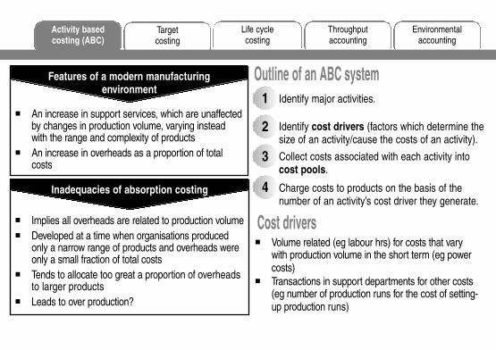
Outline of an ABC system1 Identify major activities.
2 Identify cost drivers (factors which determine thesize of an activity/cause the costs of an activity).
3 Collect costs associated with each activity intocost pools.
4 Charge costs to products on the basis of thenumber of an activity’s cost driver they generate.
Cost drivers
� An increase in support services, which are unaffectedby changes in production volume, varying insteadwith the range and complexity of products
� An increase in overheads as a proportion of totalcosts
Features of a modern manufacturingenvironment
� Implies all overheads are related to production volume� Developed at a time when organisations produced
only a narrow range of products and overheads wereonly a small fraction of total costs
� Tends to allocate too great a proportion of overheadsto larger products
� Leads to over production?
Inadequacies of absorption costing
� Volume related (eg labour hrs) for costs that varywith production volume in the short term (eg powercosts)
� Transactions in support departments for other costs(eg number of production runs for the cost of setting-up production runs)
(002)ACF5PC_CH02.qxp 07/11/2010 00:35 Page 6

2: Modern management accounting techniquesPage 7
ExampleCost of goods inwards department = $10,000
Cost driver for goods inwards activity = number ofdeliveries
During 20X0 there were 1,000 deliveries, 200 ofwhich related to product X. 4,000 units of product Xwere produced.
Cost per unit of cost driver = $10,000 ÷ 1,000 = $10
Cost of activity attributable to product X = $10 ×200 = $2,000
Cost of activity per unit of X = $2,000 ÷ 4,000 =$0.50
Merits of ABC� Simple (once information obtained)
� Focuses attention on what causes costs toincrease (cost drivers)
� Absorption rates more closely linked to causes ofoverheads because many cost drivers are used
Criticisms of ABC� More complex and so should only be introduced if
provides additional information
� Can one cost driver explain the behaviour of allitems in a cost pool?
� Cost drivers might be difficult to identify
(002)ACF5PC_CH02.qxp 07/11/2010 00:35 Page 7
Activity basedcosting (ABC)
Life cyclecosting
Environmentalaccounting
Throughputaccounting
Targetcosting
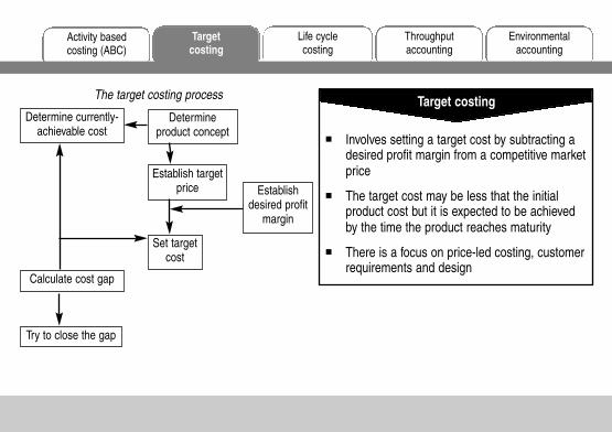
Determineproduct concept
Determine currently-achievable cost
Establish targetprice Establish
desired profitmargin
Set targetcost
Calculate cost gap
Try to close the gap
The target costing process
� Involves setting a target cost by subtracting adesired profit margin from a competitive marketprice
� The target cost may be less that the initialproduct cost but it is expected to be achievedby the time the product reaches maturity
� There is a focus on price-led costing, customerrequirements and design
Target costing
(002)ACF5PC_CH02.qxp 07/11/2010 00:35 Page 8
Activity basedcosting (ABC)
Life cyclecosting
Environmentalaccounting
Throughputaccounting
Targetcosting
2: Modern management accounting techniquesPage 9
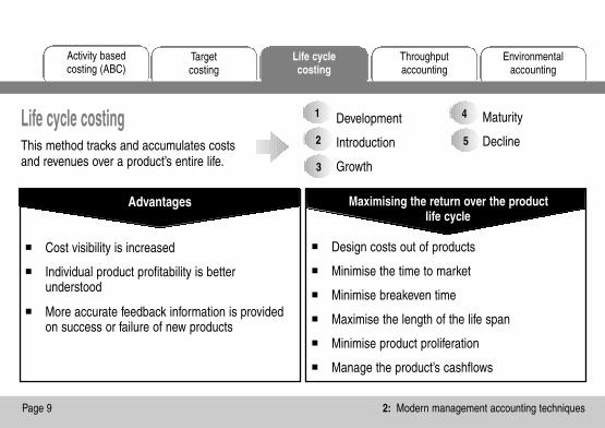
Life cycle costingThis method tracks and accumulates costsand revenues over a product’s entire life.
� Design costs out of products
� Minimise the time to market
� Minimise breakeven time
� Maximise the length of the life span
� Minimise product proliferation
� Manage the product’s cashflows
Maximising the return over the productlife cycle
� Cost visibility is increased
� Individual product profitability is betterunderstood
� More accurate feedback information is providedon success or failure of new products
Advantages
Development
Introduction
Growth
1
2
4
3
5
Maturity
Decline
(002)ACF5PC_CH02.qxp 07/11/2010 00:35 Page 9

Activity basedcosting (ABC)
Life cyclecosting
Throughputaccounting
Environmentalaccounting
Targetcosting
� In the short run, all costs except materials are fixed
� The ideal inventory level is zero and so unavoidable, idlecapacity in some operations must be accepted
� WIP is valued at material cost only, as no value is addedand no profit earned until a sale takes place
Principal concepts of throughput accounting
Throughput accounting ratio
= Return per factory hourTotal conversion cost per factory hour
An approach to production managementwhich aims to turn materials into sales asquickly as possible, thereby maximising thenet cash generated from sales. It focuses onremoving bottlenecks (binding constraints)to ensure evenness of production flow.
Theory of constraints (TOC)
Throughput accounting Developed from TOC as an alternativesystem of cost and management accountingin a JIT environment.
(002)ACF5PC_CH02.qxp 07/11/2010 00:35 Page 10

2: Modern management accounting techniquesPage 11
Activity basedcosting (ABC)
Life cyclecosting
Throughputaccounting
Environmentalaccounting
Targetcosting
Evironmental management accounting (EMA)
Typical environmental costs
� Identifying environmental costs associatedwith individual products and services canassist with pricing decisions
� Ensuring compliance with regulatorystandards
� Potential for cost savings
Why environmental costs are important
The generation and analysis of both financial andnon-financial information in order to supportenvironmental management processes.
� Consumables and raw materials
� Transport and travel
� Waste and effluent disposal
� Water consumption
� Energy
(002)ACF5PC_CH02.qxp 07/11/2010 00:35 Page 11

Environmentalaccounting
Activity basedcosting (ABC)
Life cyclecosting
Throughputaccounting
Targetcosting
Input / output analysis Environmental activity-based costing
Life-cycle costing
Operates on the principal that what comes in mustgo out. Output is split across sold and stored goodsand residual (waste). Measuring these categories inphysical quantities and monetary terms forcesbusinesses to focus on environmental costs.
Environmental costs are considered from thedesign stage right up to end-of-life costs such asdecomissioning and removal.
This may influence the design of the product itself,saving on future costs.
Environment driven costs such as costs relating toa sewage plant or an incinerator are attributed tojoint environmental cost centres.
Environmental related costs such as increaseddepreciation or higher staff wages are allocated togeneral overheads.
Material flows through an organisation are dividedinto three categories� Material� System and delivery� Disposal
The values and costs of each material flow arecalculated. This method focusses on reducingmaterial, thus reducing costs and having a positiveeffect on the environment.
Flow cost accounting
(002)ACF5PC_CH02.qxp 07/11/2010 00:35 Page 12

3: Cost volume profit (CVP analysis)
Topic List
Breakeven point
C/S ratio
Sales/product mix decisions
Target profits and margin of safety
Multi-product breakeven charts
Further aspects of CVP analysis
You need to be completely confident of the aspectsof breakeven analysis covered in your earlierstudies.
It is vital to remember that for multi-product breakevenanalysis, a constant product sales mix (whenever xunits of product A are sold, y units of product B and zunits of product C are also sold) must be assumed.
(003)ACF5PC_CH03.qxp 07/11/2010 00:39 Page 13

Further aspectsof CVP analysis
Multi-productbreakeven charts
Target profits andmargin of safety
Sales/productmix decisions
C/S ratioBreakeven point
Example (J Co) usedthroughout this chapter
(where appropriate)J Co produces and sells two products
� The M sells for $7 per unit and has atotal variable cost of $3 per unit.
� The N sells for $15 per unit an.d has atotal variable cost of $5 per unit.
For every five units of M sold, one unit of Nwill be sold.
Fixed costs total $30,000.
How to calculate a multi-product breakeven pointCalculate the contribution per unit.
Calculate the contribution per mix.
Calculate the breakeven point in number of mixes.
Calculate the breakeven point in units and revenue.
1
432
Example (J Co)M = $4 N = $10
($4 × 5) + ($10 × 1) = $30
Fixed costs ÷ contribution per mix = $30,000 ÷ $30= 1,000 mixes
M 1,000 × 5 = 5,000 units5,000 × $7 = $35,000 revenue
N 1,000 × 1 = 1,000 units1,000 × $15 = $15,000 revenue
Total breakeven revenue = $50,000
123
4
(003)ACF5PC_CH03.qxp 07/11/2010 00:39 Page 14

Further aspectsof CVP analysis
Breakeven point
Multi-productbreakeven charts
Target profits andmargin of safety
Sales/productmix decisions
C/S ratio
3: Cost volume profit (CVP analysis)Page 15
How to calculate a multi-product C/S (or profit volume or P/V) ratioCalculation of breakeven sales: approach 1
Calculate the revenue per mix.
Calculate the contribution per mix.
Calculate the average C/S ratio.
Calculate the total breakeven point.
Calculate the revenue ratio per mix.
Calculate the breakeven sales.
3
1
4
5
6
2
Example($7 × 5) + ($15 × 1) = $50
($4 × 5) + ($10 × 1) = $30
($30 ÷ $50) × 100% = 60%
Fixed costs ÷ C/S ratio = $30,000 ÷ 0.6= $50,000
($7 × 5) : ($15 × 1) = 35 : 15 or 7 : 3
M = $50,000 × 7/10 = $35,000N = $50,000 × 3/10 = $15,000_______
$50,000______________
1
2
3
4
5
6
(003)ACF5PC_CH03.qxp 07/11/2010 00:39 Page 15
Further aspectsof CVP analysis
Breakeven point
Multi-productbreakeven charts
Target profits andmargin of safety
Sales/productmix decisions
C/S ratio
4
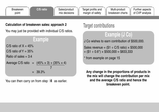
Calculation of breakeven sales: approach 2
You may just be provided with individual C/S ratios.
ExampleC/S ratio of X = 45%
C/S ratio of Y = 35%
Ratio of sales = 3:4
Average C/S ratio = (45% × 3) + (35% × 4)_________________7
= 39.3%
You can then carry on from step as earlier.
Target contributionsExample (J Co)
J Co wishes to earn contribution of $500,000.
Sales revenue = ($1 ÷ C/S ratio) × $500,000 = ($1 ÷ 0.6*) × $500,000 = $833,333
* from example on page 15
Any change in the proportions of products inthe mix will change the contribution per mix
and the average C/S ratio and hence thebreakeven point.
(003)ACF5PC_CH03.qxp 07/11/2010 00:39 Page 16

Further aspectsof CVP analysis
Breakeven point
Multi-productbreakeven charts
Target profits andmargin of safety
Sales/productmix decisions
C/S ratio
3: Cost volume profit (CVP analysis)Page 17
Most profitable mix optionSuppose J Co (from our example) has the option of changing the sales ratio to 2M to 4N. Which is the optimalmix?
Calculate breakeven point in number of mixes. Calculate breakeven point in units and revenue.21
Example (J Co)Mix 1: 1,000 mixes (calculated earlier) Mix 1: $50,000 (calculated earlier)Mix 2: Contribution per mix = ($4 × 2) + ($10 × 4) Mix 2: M 625 × 2 = 1,250 units
= $48 1,250 × $7 = $8,750 unitsBreakeven point = $30,000 ÷ $48 N 625 × 4 = 2,500 units
= 625 mixes 2,500 × $15 = $37,500 revenueTotal breakeven revenue = $46,250
Mix 2 is preferable because it requires a lower level of sales to break even (because it has a higher averagecontribution per unit sold of $48/6 = $8 (compared with $30/6 = $5 for mix 1).
21
(003)ACF5PC_CH03.qxp 07/11/2010 00:39 Page 17

Further aspectsof CVP analysis
Breakeven point
Multi-productbreakeven charts
Target profits andmargin of safety
Sales/productmix decisions
C/S ratio
Calculate the revised overall C/S ratio
Alpha Beta TotalC/S ratio (as in ) 0.5713 0.6667Market share (2/7:5/7) × 0.2857× 0.7143_____ _____ ______
0.1632 0.4762 0.6394_____ _____ ___________ _____ ______
Changing the product mixABC Co sells products Alpha and Beta in the ratio 5:1 at the same selling price per unit. Beta has a C/S ratio of66.67% and the overall C/S ratio is 58.72%. How do we calculate the overall C/S ratio if the mix is changed to 2:5?
Calculate the missing C/S ratio� Calculate original market share (Alpha 5/6,
Beta 1/6).� Calculate weighted C/S ratios.
Beta: 0.6667 × 0.1667 = 0.1111Alpha: 0.5872 – 0.1111 = 0.4761
� Calculate the missing C/S ratio.
Alpha Beta TotalC/S ratio 0.5713 * 0.6667Market share × 0.8333 × 0.1667______ ______ ______
0.4761 0.1111 0.5872______ ______ ____________ ______ ______* 0.4761/0.8333
1
1
The overall C/S ratio has increased because ofthe increase in the proportion of the mix of theBeta, which has the higher C/S ratio.
2
(003)ACF5PC_CH03.qxp 07/11/2010 00:39 Page 18

Further aspectsof CVP analysis
Breakeven point
Multi-productbreakeven charts
Target profits andmargin of safety
Sales/productmix decisions
C/S ratio
3: Cost volume profit (CVP analysis)Page 19
Target profits: approach 1Calculate the contribution per mix.
Calculate the required number of mixes.
Calculate the required number of units andsales revenue of each product.
2
1
3
Example (J Ltd)Suppose J Co wishes to earn profit of $24,900.
$30 (as earlier)
(Fixed costs + required profit)/contribution permix = $(30,000 + 24,900)/$30 = 1,830 mixes
$
M: (1,830 × 5) units for (× $7) 64,050
N: (1,830 × 1) units for (× $15) 27,450______
Total revenue 91,500
Variable costs (9,150 × $3) + (1,830 × $5) 36,600
Fixed costs 30,000______Profit 24,900____________
21
3
You should remember from your earlierstudies that the contribution required to earn
a target profit (P) = fixed costs + P.
(003)ACF5PC_CH03.qxp 07/11/2010 00:39 Page 19

Further aspectsof CVP analysis
Breakeven point
Multi-productbreakeven charts
Target profits andmargin of safety
Sales/productmix decisions
C/S ratio
Target profits: approach 2Calculate the average C/S ratio.
Calculate the required total revenue.2
1
Margin of safetyCalculate the breakeven point in revenue.
Calculate the margin of safety.2
1
Example (J Co)60% (from earlier)
Required contribution ÷ C/S ratio = (fixed costs + profit) ÷ C/S ratio= $54,900 ÷ 0.6 = $91,500
2
1
Example (J Co)Suppose J Co has budgeted sales of $62,000.
$50,000 (from earlier)
Budgeted sales – breakeven sales= $(62,000 – 50,000) = $12,000= 19.4% of budgeted sales
1
2
(003)ACF5PC_CH03.qxp 07/11/2010 00:39 Page 20

Further aspectsof CVP analysis
Breakeven point
Multi-productbreakeven charts
Target profits andmargin of safety
Sales/productmix decisions
C/S ratio
3: Cost volume profit (CVP analysis)Page 21
A multi-product breakevenchart can only be drawn on
the assumption that thesales proportions are fixed.
There are three possible approaches to preparing multi-product breakeven charts.
Output in $ sales and a constant product mixProducts in sequenceOutput in tems of % of forecast sales and a constant product mix
Breakeven chart
123
(003)ACF5PC_CH03.qxp 07/11/2010 00:39 Page 21

Further aspectsof CVP analysis
Breakeven point
Multi-productbreakeven charts
Target profits andmargin of safety
Sales/productmix decisions
C/S ratio
P/V chartSuppose J’s sales budget is 6,000 units of Mand 1,200 units of N.
Revenue (6,000 × $7 + 1,200 × $15) = $60,000
Variable costs (6,000 × $3 + 1,200 × $5) =$24,000
On the chart, products are shown individually,from left to right, in order of size of decreasingC/S ratio.
Cum CumC/S ratio sales profit
$’000 $’000N 66.67% 18 *(18)M 57.14% 60 6
* (1,200 × $15) – (12,000 × $5) – $30,000
(003)ACF5PC_CH03.qxp 07/11/2010 00:39 Page 22
3: Cost volume profit (CVP analysis)Page 23
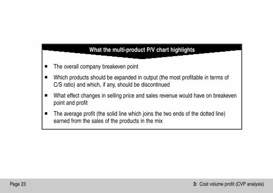
� The overall company breakeven point
� Which products should be expanded in output (the most profitable in terms of C/S ratio) and which, if any, should be discontinued
� What effect changes in selling price and sales revenue would have on breakevenpoint and profit
� The average profit (the solid line which joins the two ends of the dotted line)earned from the sales of the products in the mix
What the multi-product P/V chart highlights
(003)ACF5PC_CH03.qxp 07/11/2010 00:39 Page 23

Further aspectsof CVP analysis
Breakeven point
Multi-productbreakeven charts
Target profits andmargin of safety
Sales/productmix decisions
C/S ratio
� Graphical representation of cost and revenuedata can be more easily understood by non-financial managers
� Highlighting the breakeven point and margin ofsafety gives managers an indication of the levelof risk involved
Advantages of CVP analysis
� It is assumed that fixed costs are the same intotal and variable costs are the same per unit atall levels of output
� It is assumed that sales prices will be constantat all levels of activity
� Production and sales are assumed to be thesame
� Uncertainty in estimates of fixed costs and unitvariable costs is often ignored
Limitations of CVP analysis
(003)ACF5PC_CH03.qxp 07/11/2010 00:39 Page 24

4: Limiting factor analysis
Topic List
Formulating the problem
Finding the solution
Slack, surplus and shadow prices
Limiting factor analysis is a technique used to determinean optimum product mix which will maximise contributionand profit.
Linear programming is used where there is more thanone resource constraint.
(004)ACF5PC_CH04.qxp 07/11/2010 00:44 Page 25

Slack, surplus andshadow prices
Finding the solution
Formulatingthe problem
ExampleA company makes two products, standard and deluxe.
Relevant data are as follows.
Standard Deluxe Availability per month
Profit per unit $15 $20Labour hours
per unit 5 10 4,000Kgs of material
per unit 10 5 4,250
Step 1. Define variables
� Let x = number of standards producedeach month
� Let y = number of deluxes producedeach month
Step 2. Establish constraints
� Labour 5x + 10y ≤ 4,000� Material 10x + 5y ≤ 4,250� Non-negativity x ≥ 0, y ≥ 0
Step 3. Construct objective function
� Profit (P) = 15x + 20y
(004)ACF5PC_CH04.qxp 07/11/2010 00:44 Page 26

Slack, surplus andshadow prices
Finding the solution
Formulatingthe problem
4: Limiting factor analysisPage 27
There are two methods you need to know about whenfinding the solution to a linear programming problem.
� Graphical method
� Using equations
Graphical methodStep 1. Graph the constraints
Labour 5x + 10y = 4,000if x = 0, y = 400if y = 0, x = 800
Material 10x + 5y = 4,250if x = 0, y = 850if y = 0, x = 425
150
400
850
200 425 800
Material
Feasible region
Labour
y
x
(004)ACF5PC_CH04.qxp 07/11/2010 00:44 Page 27

Slack, surplus andshadow prices
Finding the solution
Formulatingthe problem
Using equations� Graph constraints and establish
feasible area
� Determine all possible intersectionpoints of constraints and axesusing simultaneous equations
� Calculate profit at each intersectionpoint to determine which is theoptimal solution
Step 2. Establish the feasible area/region
This is the area where all inequalities are satisfied (areaabove x axis and y axis (x ≥ 0, y ≥ 0), below materialconstraint (≤) and below labour constraint (≤)
Step 3. Add an iso-profit line
Suppose P = $3,000 so that if P = 15x + 20y then if x =0, y = 150 and if y = 0, x = 200 and (sliding your ruleracross the page if necessary) find the point furthest fromthe origin but still in the feasible area
Step 4. Use simultaneous equations to find the x and ycoordinates at the optimal solution, the intersection of thematerial and labour constraints (x = 300, y = 250)
(004)ACF5PC_CH04.qxp 07/11/2010 00:44 Page 28
Slack, surplus andshadow prices
Finding the solution
Formulatingthe problem
4: Limiting factor analysisPage 29
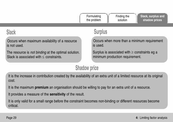
SlackOccurs when maximum availability of a resourceis not used.
The resource is not binding at the optimal solution.Slack is associated with ≤ constraints.
Surplus
Shadow price
Occurs when more than a minimum requirementis used.
Surplus is associated with ≥ constraints eg aminimum production requirement.
It is the increase in contribution created by the availability of an extra unit of a limited resource at its originalcost.
It is the maximum premium an organisation should be willing to pay for an extra unit of a resource.
It provides a measure of the sensitivity of the result.
It is only valid for a small range before the constraint becomes non-binding or different resources becomecritical.
(004)ACF5PC_CH04.qxp 07/11/2010 00:44 Page 29

Notes
(004)ACF5PC_CH04.qxp 07/11/2010 00:44 Page 30

5: Pricing decisions
Topic List
Pricing policy and the market
Demand
Profit maximisation
Price strategies
Pricing of an organisation’s products or services is anessential part of its profitability and survival.
There are many factors influencing prices andorganisations may have different price strategies.
(005)ACF5PC_CH05.qxp 07/11/2010 00:45 Page 31
Pricestrategies
Profitmaximisation
DemandPricing policyand the market
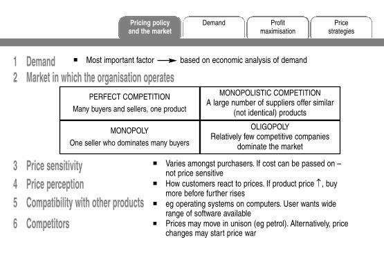
1 Demand2 Market in which the organisation operates
3 Price sensitivity 4 Price perception 5 Compatibility with other products
6 Competitors
� Most important factor based on economic analysis of demand
� Varies amongst purchasers. If cost can be passed on –not price sensitive
� How customers react to prices. If product price ↑, buymore before further rises
� eg operating systems on computers. User wants widerange of software available
� Prices may move in unison (eg petrol). Alternatively, pricechanges may start price war
PERFECT COMPETITION
Many buyers and sellers, one product
MONOPOLY
One seller who dominates many buyers
MONOPOLISTIC COMPETITIONA large number of suppliers offer similar
(not identical) products
OLIGOPOLYRelatively few competitive companies
dominate the market
(005)ACF5PC_CH05.qxp 07/11/2010 00:45 Page 32

5: Pricing decisionsPage 33
7 Competition fromsubstitute products
8 Suppliers
9 Inflation
10 Quality
11 Incomes
12 Ethics
� eg train prices ↑, competitionfrom coach or air travel Demand is the most important factor
influencing the price of a product
Price
Demand
Demand increases as prices are lowered
� If organisation’s product price ↑,suppliers may seek price rise in supplies
� Price changes to reflect increase in priceof supplies
� Customers tend to judge quality by price
� When household incomes rising, price notso important. When falling, important
� Exploit short-term shortages throughhigher prices?
(005)ACF5PC_CH05.qxp 07/11/2010 00:45 Page 33

Pricestrategies
Profitmaximisation
DemandPricing policyand the market
Price elasticity of demand (ηη)A measure of the extent of change in market demand for a good, in response to a change in its price
= change in quantity demanded, as a % of demand ÷ change in price, as a % of price
Inelastic demand� η < 1� Steep demand curve� Demand falls by a smaller % than % rise in price� Pricing decision: increase prices
Elastic demand� η > 1� Shallow demand curve� Demand falls by a larger % than % rise in price� Pricing decision: decide whether change in cost
will be less than change in revenue
� The price of the good
� The price of other goods
� The size and distribution of household incomes
� Tastes and fashion
� Expectations
� Obsolescence
Variables which influence demand
(005)ACF5PC_CH05.qxp 07/11/2010 00:45 Page 34

5: Pricing decisionsPage 35
Demand and the individual firm The demand equation
The total cost function
Influenced by:
� Product life cycle� Quality� Marketing
– price– product– place– promotion
The equation for the demand curve is
P = a – bQP is the priceQ is the quantity demandeda is the price at which demand = 0
b is quantity in change
price in change
Cost behaviour can be modelled using equations and linear regression analysis. A volume-based discountis a discount given for buying in bulk which reduces the variable cost per unit and therefore the slope of thecost function is less steep.
(005)ACF5PC_CH05.qxp 07/11/2010 00:45 Page 35
Profitmaximisation
Pricestrategies
DemandPricing policyand the market
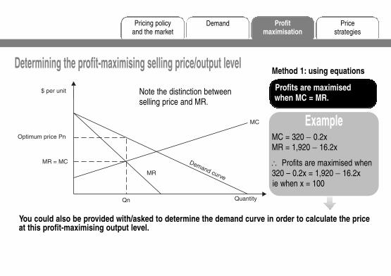
Determining the profit-maximising selling price/output levelMethod 1: using equations
ExampleMC = 320 − 0.2xMR = 1,920 − 16.2x
∴ Profits are maximised when320 – 0.2x = 1,920 − 16.2xie when x = 100
You could also be provided with/asked to determine the demand curve in order to calculate the priceat this profit-maximising output level.
Note the distinction betweenselling price and MR.
Profits are maximisedwhen MC = MR.
(005)ACF5PC_CH05.qxp 07/11/2010 00:45 Page 36
5: Pricing decisionsPage 37
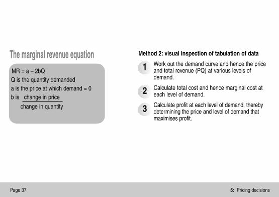
Method 2: visual inspection of tabulation of data
Work out the demand curve and hence the priceand total revenue (PQ) at various levels ofdemand.
Calculate total cost and hence marginal cost ateach level of demand.
Calculate profit at each level of demand, therebydetermining the price and level of demand thatmaximises profit.
2
1
3
The marginal revenue equationMR = a – 2bQQ is the quantity demandeda is the price at which demand = 0b is change in price
change in quantity
(005)ACF5PC_CH05.qxp 07/11/2010 00:45 Page 37

Profitmaximisation
Pricestrategies
DemandPricing policyand the market
In practice, cost is one of the most important influences on price � Full cost-plus
� Marginal cost-plus
Full cost-plus pricing
is a method ofdetermining the salesprice by calculating thefull cost of the productand adding a percentagemark-up for profit.
ExampleVariable cost of production = $4 per unitFixed cost of production = $3 per unitPrice is to be 40% higher than full cost
Full cost per unit = $(4 + 3) = $7
Price = $7 ×
= $9.80100
140%
AdvantagesQuick, simple, cheap methodEnsures company covers fixedcosts
DisadvantagesDoesn’t recognise profit-maximising combination of priceand demandBudgeted output needs to beestablishedSuitable basis for overheadabsorption needed
��
�
�
�
(005)ACF5PC_CH05.qxp 07/11/2010 00:45 Page 38
5: Pricing decisionsPage 39
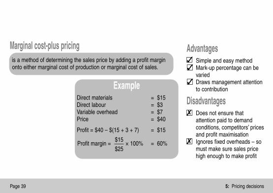
Marginal cost-plus pricingis a method of determining the sales price by adding a profit marginonto either marginal cost of production or marginal cost of sales.
AdvantagesSimple and easy methodMark-up percentage can bevariedDraws management attentionto contribution
DisadvantagesDoes not ensure thatattention paid to demandconditions, competitors’ pricesand profit maximisationIgnores fixed overheads – somust make sure sales pricehigh enough to make profit
ExampleDirect materials = $15Direct labour = $3Variable overhead = $7Price = $40
Profit = $40 – $(15 + 3 + 7) = $15
Profit margin = × 100% = 60%$25
$15
��
�
�
�
(005)ACF5PC_CH05.qxp 07/11/2010 00:45 Page 39

Profitmaximisation
Pricestrategies
DemandPricing policyand the market
Other pricing strategies� New products
� Market penetration
low prices when product launched
� Market skimming
charge high prices when product launched
� Complementary product pricing use a ‘loss leader’
� Product-line pricing prices reflect cost proportions or demand relationships
� Volume discounting reduction in price for large purchases
� Relevant cost pricing for special orders determine a minimum price
� Price discrimination the practice of charging different prices for the same product for different groups of buyers
(005)ACF5PC_CH05.qxp 07/11/2010 00:45 Page 40

6: Short-term decisions
Topic List
Relevant costs
Make or buy decisions
Further processing and shutdown
The overriding requirement of information needed tomake decisions is relevance. Decision-making questionsrequire a discussion of non-quantifiable factors as well ascalculations to support a particular option.
(006)ACF5PC_CH06.qxp 07/11/2010 00:50 Page 41

Relevant costs
Further processingand shutdown
Make or buydecisions
Relevant costs
is a cost which would not be incurred ifthe activity to which it related did notexist.
Avoidable costis the benefit which would have beenearned but which has been given up, bychoosing one option instead of another.
Opportunity cost
is the difference in thecost of alternatives.
Differential costis an item of expenditure which can be directlyinfluenced by a given manager within a given time span.
Controllable cost
Relevant costs are� future� incremental� cash flows
(006)ACF5PC_CH06.qxp 07/11/2010 00:50 Page 42

6: Short-term decisionsPage 43
Non-relevant costs
Sunk cost Fixed costs
Direct and indirect costs may be relevant or irrelevant depending on the situation.
Relevant cost of materials� Not owned � current replacement cost
� Owned � will be replaced � current replacement cost
� will not be replaced
� higher of current resale value andvalue if put to an alternative use
Relevant cost of labour� Direct labour cost plus
contribution lost by divertinglabour to make another product
is a past (historical) cost which is notdirectly relevant in decision making.
Unless given an indication to the contrary, assume fixedcosts are irrelevant and variable costs are relevant.
(006)ACF5PC_CH06.qxp 07/11/2010 00:50 Page 43

Further processingand shutdown
Make or buydecisions
Relevant costs
A make or buy problem involves a decision by an organisation about whether it should make a product/carryout an activity with its own internal resources, or whether it should pay another organisation to make theproduct/carry out the activity.
No scarce resource
With scarce resources
Relevant costs are the differential costs between the two options
Where a company must subcontract work to make up a shortfall in its ownproduction capacity, its total costs are minimised by subcontracting work which addsthe least extra marginal cost per unit of scarce resource saved by subcontracting.
(006)ACF5PC_CH06.qxp 07/11/2010 00:50 Page 44

6: Short-term decisionsPage 45
Example (limited labour time)A B
Variable cost of making $16 $14Variable cost of buying $20 $19Extra variable cost of buying $4 $5
Labour hours saved by buying 2 2Extra variable cost of buyingper hour saved $2 $2.50
Priority for making in-house 2nd 1st
Outsourcing
Advantages
Superior quality andefficiency
Capital is freed up
Greater capacity andflexibility to cope withchanges in demand
Disadvantages
Reliability of supplier
Loss of control andflexibility
Effect on existingworkforce
is the use of external suppliers for finishedproducts, components or services
��
�
�
�
�
(006)ACF5PC_CH06.qxp 07/11/2010 00:50 Page 45

Further processingand shutdown
Make or buydecisions
Relevant costs
Further processing decisions
Any short-term decision must consider qualita-tive factors related to the impact on employees,customers, competitors and suppliers
� Whether or not to shut down afactory/department/product line because it ismaking a loss or too expensive to run
� Whether closure should be permanent ortemporary
Shut down decisions
Calculate what is earned by the process atpresent (perhaps in comparison with others).Calculate what will be the financialconsequences of closing down (selling machines,redundancy costs etc).Compare the results and act accordingly.Bear in mind that some fixed costs may nolonger be incurred if the decision is to shut downand they are therefore relevant to the decision.
4
3
2
1
A joint product should be processed further pastthe split-off point if sales revenue minus furtherprocessing costs exceeds its sales revenue at thesplit-off point.
The apportionment of joint processing costs isirrelevant to the decision.
(006)ACF5PC_CH06.qxp 07/11/2010 00:50 Page 46

7: Risk and uncertainty
Topic List
Risk and uncertainty
Expected values
Decision rules
Decision trees
Value of information
Sensitivity analysis
Simulation models
This chapter covers some of the techniques that themanagement accountant can use to take account of anyrisk or uncertainty surrounding decisions.
(007)ACF5PC_CH07.qxp 07/11/2010 00:53 Page 47

Sensitivityanalysis
Expectedvalues
Simulationmodels
Decisionrules
Decisiontrees
Value ofinformation
Risk anduncertainty
RiskInvolves situations or events which may or maynot occur, but whose probability of occurrence canbe calculated statistically and the frequency oftheir occurrence predicted from past records
UncertaintyInvolves events whose outcome cannot bepredicted with statistical confidence.
Market research can be used to reduceuncertainty.
Attitude to riskRisk seeker A decision maker interested in the
best outcomes no matter how smallthe chance that they may occur
Risk neutral A decision maker concerned withwhat will be the most likely outcome
Risk averse A decision maker who acts on theassumption that the worst outcomemight occur
(007)ACF5PC_CH07.qxp 07/11/2010 00:53 Page 48

7: Risk and uncertaintyPage 49
Expected values (EV)indicate what an outcome is likely to be in the longterm with repetition.
ExampleIf contribution could be $10,000, $20,000 or$30,000 with respective probabilities of 0.3, 0.5and 0.2, the EV of contribution =
$ $10,000 × 0.3 3,000$20,000 × 0.5 10,000$30,000 × 0.2 6,000_____EV of contribution 19,000__________
The expected value will never actually occur.
Sensitivityanalysis
Expectedvalues
Simulationmodels
Decisionrules
Decisiontrees
Value ofinformation
Risk anduncertainty
(007)ACF5PC_CH07.qxp 07/11/2010 00:53 Page 49

MaximinThe ‘play it safe’ basis for decision making.
Choose the least unattractive worst outcome.
Maximax
Minimax regretThe ‘opportunity loss’ basis for decision making.Minimise the regret from making the wrongdecision.
Different people will reach different decisions onthe same problem.
� defensive and conservative
� ignores probability of each differentoutcome taking place
� ignores probabilities� over optimistic
Looks at the best possible result.
Sensitivityanalysis
Expectedvalues
Simulationmodels
Decisionrules
Decisiontrees
Value ofinformation
Risk anduncertainty
(007)ACF5PC_CH07.qxp 07/11/2010 00:53 Page 50

7: Risk and uncertaintyPage 51
Sensitivityanalysis
Expectedvalues
Simulationmodels
Decisionrules
Decisiontrees
Value ofinformation
Risk anduncertainty
Preparation
Start with a (labelled) decision point.2
Add branches for each option/alternative.3
If the outcome of an option is 100% certain,the branch for that alternative is complete.
4
If the outcome of an option is uncertain(because there are a number of possibleoutcomes), add an outcome point.
5
For each possible outcome, add a branch(with the relevant probability) to the outcomepoint.
6
Always work chronologically from left toright.
1
A
X
YA
X
YAB
X
YA 0.7
0.3B
(007)ACF5PC_CH07.qxp 07/11/2010 00:53 Page 51

Sensitivityanalysis
Expectedvalues
Simulationmodels
Decisionrules
Decisiontrees
Value ofinformation
Risk anduncertainty
Evaluating the decisionWork from right to left and calculate the EV of revenue/cost/contribution/profit at each outcome point (rollbackanalysis).
ExampleAs a result of an increase in demand for a town's car parking facilities, the owners of a car park are reviewingtheir business operations. A decision has to be made now to select one of the following three options for thenext year.
Option 1: Make no change. Annual profit is $100,000. There is little likelihood that this will provoke newcompetition this year.
Option 2: Raise prices by 50%. If this occurs there is a 75% chance that an entrepreneur will set up incompetition this year. The Board's estimate of its annual profit in this situation would be as follows.
2A WITH a new competitor 2B WITHOUT a new competitorProbability Profit Probability Profit
0.3 $150,000 0.7 $200,0000.7 $120,000 0.3 $150,000
(007)ACF5PC_CH07.qxp 07/11/2010 00:53 Page 52

7: Risk and uncertaintyPage 53
Option 3: Expand the car park quickly, at a cost of $50,000, keeping prices the same. The profits are thenestimated to be like 2B above, except that the probabilities would be 0.6 and 0.4 respectively.
At C, expected profit = (150 × 0.3) + (120 × 0.7) = $129,000At D, expected profit = (200 × 0.7) + (150 × 0.3) = $185,000At B, expected profit = (129 × 0.75) + (185 × 0.25) = $143,000At E, expected profit = (200 × 0.6) + (150 × 0.4) = $180,000
Option Expected profit$'000
1 1002 1433 (180 – 50) 130
(007)ACF5PC_CH07.qxp 07/11/2010 00:53 Page 53

Sensitivityanalysis
Expectedvalues
Simulationmodels
Decisionrules
Decisiontrees
Value ofinformation
Risk anduncertainty
The value of perfect informationWork out the EVs of all options and see whichis best.
See what decision would be taken with perfectinformation (if all the outcomes were known inadvance with certainty) and calculate the EV.
The value of perfect information (the amountyou would be willing to pay to obtain it)= EV of the action you would take with theinformation – EV without the information.
1
3
2
ExampleProfit if strong Profit/(loss) if
demand weak demandOption A $4,000 $(1,000)Option B $1,500 $600Probability 0.3 0.7
EV of A = 4,000 × 0.3 + (1,000) × 0.7 = $500EV of B = 1,500 × 0.3 + 600 × 0.7 = $870
∴ Choose B
With perfect information, if demand is strong choose Abut if demand is weak choose B.
∴ EV with perfect information = 0.3 × 4,000 + 0.7 × 600= $1,620
∴ Value of perfect information = $(1,620 – 870)= $750
Alternatively a decision tree can be used.
(007)ACF5PC_CH07.qxp 07/11/2010 00:53 Page 54
7: Risk and uncertaintyPage 55
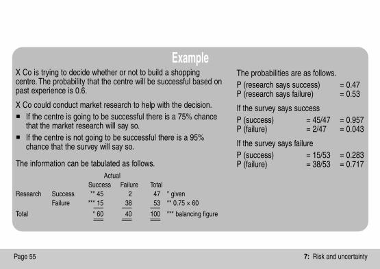
ExampleThe probabilities are as follows.P (research says success) = 0.47P (research says failure) = 0.53
If the survey says successP (success) = 45/47 = 0.957P (failure) = 2/47 = 0.043
If the survey says failureP (success) = 15/53 = 0.283P (failure) = 38/53 = 0.717
X Co is trying to decide whether or not to build a shoppingcentre. The probability that the centre will be successful based onpast experience is 0.6.
X Co could conduct market research to help with the decision.� If the centre is going to be successful there is a 75% chance
that the market research will say so.� If the centre is not going to be successful there is a 95%
chance that the survey will say so.
The information can be tabulated as follows.Actual
Success Failure TotalResearch Success ** 45 2 47 * given
Failure *** 15 38 53 ** 0.75 × 60___ ___ ___Total * 60 40 100 *** balancing figure___ ___ ______ ___ ___
(007)ACF5PC_CH07.qxp 07/11/2010 00:53 Page 55

The essence of all approaches to sensitivity analysis is to carry outcalculations with one set of values for the variables and then substitute otherpossible values for the variables to see how this effects the overall outcome.
Approach 1 Estimate by how much a
variable would need to differ from its estimatedvalue before the decision would change.
Approach 2 Estimate whether a
decision would change if a variablewas X% higher than expected.
Approach 3Estimate by how much avariable would need todiffer before a decisionmaker was indifferentbetween two options.
ExampleOption 2 is $10,000 more expensive than option 1 and involves taking adiscount of 10% from a supplier from whom you purchase $50,000 ofgoods (before discount) pa for 4 years. Ignore the time value of money.Discount needs to be $10,000 (difference) + $20,000 (current discount) ifoption 2 is as good as option 1.∴ (4 × $50,000) × X% = $30,000∴ X = 15% (rate at which you are indifferent between the two options)
Sensitivity analysis is oneform of ‘what-if?’ analysis
Sensitivityanalysis
Expectedvalues
Simulationmodels
Decisionrules
Decisiontrees
Value ofinformation
Risk anduncertainty
(007)ACF5PC_CH07.qxp 07/11/2010 00:53 Page 56

7: Risk and uncertaintyPage 57
Simulation models ExampleNumbers
Daily demand Probability assignedUnits17 0.15 00-1418 0.45 15-5919 0.40 60-99
1.00
Random numbers for a simulation overthree days are 761301.
RandomDay number Demand
1 76 192 13 173 01 17
can be used to deal with decision problemsinvolving a number of uncertain variables.
Random numbers are used to assign values to thevariables.
Sensitivityanalysis
Expectedvalues
Simulationmodels
Decisionrules
Decisiontrees
Value ofinformation
Risk anduncertainty
(007)ACF5PC_CH07.qxp 07/11/2010 00:53 Page 57

Notes
(007)ACF5PC_CH07.qxp 07/11/2010 00:53 Page 58
8: Objectives of budgetary control
Topic List
Objectives
Planning and control
Behavioural aspects of budgeting
Budgeting is an important aspect of many accountants’lives and budgetary control and its behaviouralimplications are essential aspects to understand.
(008)ACF5PC_CH08.qxp 07/11/2010 00:55 Page 59

Planning and control
Behavioural aspectsof budgeting
Objectives
Corporate objectives Conflicting objectivesare set as part of the corporate planning processwhich is concerned with selecting strategies toachieve objectives.
Goal congruenceexists when managers working in their own best interests also act in harmony with organisational goals.
Corporate objectives may conflict with divisionalobjectives
Setting objectives is a political process usingbargaining
Conflict is resolved using prioritisation,compromise, negotiation and satisfying
(008)ACF5PC_CH08.qxp 07/11/2010 00:55 Page 60

Planning andcontrol
Behavioural aspectsof budgeting
Objectives
8: Objectives of budgetary controlPage 61
The planning and control cycle
Planningprocess
Controlprocess
Step 1
Step 2
Step 3
Step 4
Step 5
Step 6
Step 7
Identify objectives
Identify alternative courses of action(strategies) which might contributetowards achieving the objectives
Evaluate each strategy
Choose alternativecourses of action
Implement the long-termplan in the form of the annual budget
Measure actual resultsand compare with the plan
Respond todivergences from plan
(008)ACF5PC_CH08.qxp 07/11/2010 00:55 Page 61
Planning and control
Behavioural aspectsof budgeting
Objectives
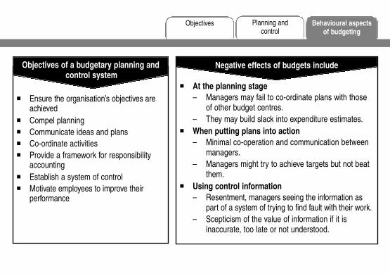
� Ensure the organisation’s objectives areachieved
� Compel planning� Communicate ideas and plans� Co-ordinate activities� Provide a framework for responsibility
accounting� Establish a system of control� Motivate employees to improve their
performance
Objectives of a budgetary planning andcontrol system
� At the planning stage– Managers may fail to co-ordinate plans with those
of other budget centres.– They may build slack into expenditure estimates.
� When putting plans into action– Minimal co-operation and communication between
managers.– Managers might try to achieve targets but not beat
them.� Using control information
– Resentment, managers seeing the information aspart of a system of trying to find fault with their work.
– Scepticism of the value of information if it isinaccurate, too late or not understood.
Negative effects of budgets include
(008)ACF5PC_CH08.qxp 07/11/2010 00:55 Page 62

8: Objectives of budgetary controlPage 63
Budgets as targetsCan budgets, as targets, motivate managers to achieve a high level of performance?� Ideal standards are demotivating because adverse efficiency variances are always reported� Low standards are demotivating because there is no sense of achievement in attainment, no impetus to try
harder� Normal levels of attainment can encourage budgetary slack
To ensure managers are properly motivated, two budgets can be used.� One for planning and decision making, based on reasonable expectations (expectations budget)� One for motivational purposes, with more difficult targets (aspirations budget)
Budgetary slackthe difference between the minimum necessary costsand the costs built into the budget or actually incurred
Managers might deliberately overestimate costsand underestimate sales so that they will not beblamed for overspending and poor results.
(008)ACF5PC_CH08.qxp 07/11/2010 00:55 Page 63

Planning and control
Behavioural aspectsof budgeting
Objectives
Participation
� Imposed (from the top down)� Participative (from the bottom up)� Negotiated
Budget-setting styles
Advantages of participative approach include
More realistic budgets
Co-ordination, morale and motivation improved
Increased management commitment to objectives
Disadvantages of participative approach include
More time-consuming
Budgetary slack may be introduced
Does not suit some employees
�
�
�
�
�
�
In practice final budgets are likely to liebetween what top managemetn would really likeand what junior managers believe is feasible.
If employees feel they do not have the necessary skills,think that the budget will be used against them orcomplain thet are too busy, participation could be anadded pressure rather than an opportunity.
(008)ACF5PC_CH08.qxp 07/11/2010 00:55 Page 64

9: Budgetary systems
Topic List
Traditional budgetary systems
Zero based budgeting (ZBB)
Other systems
Budgeting issues
There are a range of budgetary systems and types whichcan be used. The traditional approach of incrementalbudgeting is not always appropriate or useful.
(009)ACF5PC_CH09.qxp 07/11/2010 00:56 Page 65

Othersystems
Traditionalbudgetary systems
Budgeting issues
Zero basedbudgeting (ZBB)
These are budgets which, by recognising differentcost behaviour patterns, change as activity levelschange.
� At the planning stage, flexible budgets can bedrawn up to show the effect of the actualvolumes of output and sales differing frombudgeted volumes.
� At the end of a period, actual results can becompared to a flexed budget (what resultsshould have been at actual output and salesvolumes) as a control procedure.
Flexible budgets
These are prepared on the basis of an estimatedvolume of production and an estimated volume ofsales. No variants of the budget are made to coverthe event that actual and budgeted activity levelsdiffer and they are not adjusted (in retrospect) toreflect actual activity levels.
Fixed budgets
This involves adding a certain percentage to lastyear’s budget to allow for growth and inflation. Itencourages slack and wasteful spending to creepinto budgets.
Incremental budgeting
(009)ACF5PC_CH09.qxp 07/11/2010 00:56 Page 66

Othersystems
Traditionalbudgetary systems
Budgeting issues
Zero basedbudgeting (ZBB)
9: Budgetary systemsPage 67
ZBB
This approach treats the preparation of the budget for each period as an independent planning exercise: the initial budgetis zero and every item of expenditure has to be justified in its entirety to be included.
Three-step approach to ZBBDefine decision packages(description of a specific activityso that it can be evaluated andranked).
Evaluate and rank packages onthe basis of their benefit to theorganisation.
Allocate resources according tothe funds available and theranking of packages.
Mutually exclusive packages
Incrementalpackages
1 2 3
(009)ACF5PC_CH09.qxp 07/11/2010 00:56 Page 67

Othersystems
Traditionalbudgetary systems
Budgeting issues
Zero basedbudgeting (ZBB)
� Involves time and effort
� Can cause suspicion when introduced
� Costs and benefits of different alternative coursesof action can be difficult to quantity
� Ranking can prove problematic
Disadvantages of ZBB
� Identifies and removes inefficient and/or obsoleteoperations
� Provides a psychological impetus to employees toavoid wasteful expenditure
� Leads to a more efficient allocation of resources
Advantages of ZBB
At its simplest, ABB involves the use of costs determinedusing ABC in budgets. More formally, it involves definingthe activities that underlie the figures in each functionand using the level of activity to decide how muchresource should be allocated, how well it is beingmanaged and to explain variances from budget.
Activity based budgeting (ABB)
(009)ACF5PC_CH09.qxp 07/11/2010 00:56 Page 68
Othersystems
Traditionalbudgetary systems
Budgeting issues
Zero basedbudgeting (ZBB)
9: Budgetary systemsPage 69
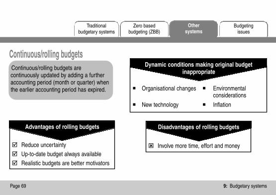
Continuous/rolling budgetsContinuous/rolling budgets arecontinuously updated by adding a furtheraccounting period (month or quarter) whenthe earlier accounting period has expired. � Organisational changes � Environmental
considerations
� New technology � Inflation
Dynamic conditions making original budgetinappropriate
� Reduce uncertainty
� Up-to-date budget always available
� Realistic budgets are better motivators
Advantages of rolling budgets
� Involve more time, effort and money
Disadvantages of rolling budgets
(009)ACF5PC_CH09.qxp 07/11/2010 00:56 Page 69

Budgetingissues
Othersystems
Traditionalbudgetary systems
Zero basedbudgeting (ZBB)
Sources of budget information Difficulties of changing budgetary practices
Allowing for uncertainty
� Past data
� Sales forecasts
� Production department costing information
� Resistance by employees
� Loss of control
� Time consuming and expensive training
� Cost of implementation
� Lack of accounting information and systems inplace
� Flexible budgeting
� Rolling budgets
� Probabilistic budgeting
� Sensitivity analysis
(009)ACF5PC_CH09.qxp 07/11/2010 00:56 Page 70

10: Quantitative analysis in budgeting
Topic List
Analysing fixed and variable costs
Forecasting techniques
Learning curves
Expected values and spreadsheets
This chapter looks at where the figures which go intobudgets come from. There are a number of quantitativetechniques which are used in budgeting.
(010)ACF5PC_CH10.qxp 07/11/2010 00:58 Page 71

Forecasting techniques
Learningcurves
Expected valuesand spreadsheets
Analysing fixed andvariable costs
The high-low method may give inaccurate cost estimations as it assumes costs at the extremes ofactivity are representative.
The fixed and variable elements of semi-variablecosts can be determined by the high-low method.
Step 1. Review past records of costs
Step 2. Determine
Select period with highest activity levelSelect period with lowest activity level
Total cost at high activity level (TCH)
Total cost at low activity level (TCL)
Total units at high activity level (TUH)
Total units at low activity level (TUL)
Step 3. Calculate variable cost per unit =
Step 4. Determine fixed costs by substituting variable cost per unit = TCH – (TUH x VC per unit)
TUL–TUH
TCL–TCH
(010)ACF5PC_CH10.qxp 07/11/2010 00:58 Page 72

10: Quantitative analysis in budgetingPage 73
Linear regression analysis finds the equation of thestraight line (line of best fit) which has the generalform y = a +bxwhere y = dependent variable = total cost
x = independent variable = level of activitya = intercept of line on y axis = fixed costb = gradient of line = variable cost per unit
Historical data (adjusted for inflation) provide readingsfor x and y. These readings are then substituted intoformulae for a and b.
nΣΣxy – ΣΣxΣΣy ΣΣy bΣΣxb = ____________ and a = ____ – _____nΣΣx2 – (ΣΣx)2 n n
where n = number of pairs of data for x and y.Once the equation has been determined, a value for x(activity level) can be substituted into the equation and avalue for y (total cost at that activity level) forecast.
The formulae for a and b will be provided in the exam.
� A linear cost function is assumed
� Historical cost data is accurately recorded
� There are 10+ pairs of data
� The activity levels in the historical data cover the fullnormal range of activity
� Data is adjusted to account for inflation
� Past conditions are indicative of future conditions
� The value of y can be predicted from the value of x
Conditions necessary for the use of linearregression analysis
(010)ACF5PC_CH10.qxp 07/11/2010 00:58 Page 73
Forecasting techniques
Learningcurves
Expected valuesand spreadsheets
Analysing fixed andvariable costs
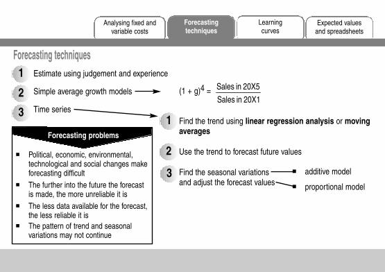
Forecasting techniquesEstimate using judgement and experience
Simple average growth models
Time series
1
2
3
(1 + g)4 =
Find the trend using linear regression analysis or movingaverages
Use the trend to forecast future values
Find the seasonal variationsand adjust the forecast values
20X1 in Sales
20X5 in Sales
� Political, economic, environmental, technological and social changes makeforecasting difficult
� The further into the future the forecastis made, the more unreliable it is
� The less data available for the forecast,the less reliable it is
� The pattern of trend and seasonalvariations may not continue
Forecasting problems
� additive model
� proportional model
1
2
3
(010)ACF5PC_CH10.qxp 07/11/2010 00:58 Page 74

Learningcurves
Analysing fixed andvariable costs
Expected valuesand spreadsheets
Forecastingtechniques
10: Quantitative analysis in budgetingPage 75
TheoryAs cumulative output doubles, thecumulative average time per unitproduced falls to a fixed percentage of theprevious cumulative average time per unit.
Note that cumulative average time = averagetime per unit for all units produced so far,back to and including the first unit made.
� Product made largely by labour effort� Brand new or relatively short-lived
product� Complex product made in small
quantities for special orders
When does learning curve theoryapply?
ExampleAssume a 90% learning effect applies.
CumulativeCumulative average time Total time
output per unit required Incremental time takenUnits Hours Hours Total hours Hours/unit
1 50.00 (× 1) 50.02* (× 90%) 45.00 (× 2) 90.0 40.0 (÷ 1) 40.04* (× 90%) 40.50 (× 4) 162.0 72.0 (÷ 2) 36.08* (× 90%) 36.45 (× 8) 291.6 129.6 (÷ 4) 32.4
* Output doubled each time
(010)ACF5PC_CH10.qxp 07/11/2010 00:58 Page 75

Forecasting techniques
Learningcurves
Expected valuesand spreadsheets
Analysing fixed andvariable costs
Formula for the learning curveThe learning effect can be shown as a learningcurve.
The formula for learning curve (a) shown above isY = aXb
where Y = average cost per unit
X = the number of units made so far
a = the cost of the first unit
b = the learning coefficient or index= log of learning rate / log of 2
This formula will be provided in the exam if it is needed.
� As the learning effect is a function of labour,only labour costs and other variable costsdirectly dependent on labour are affected
� Materials should not be affected unless early onin the learning process they are usedinefficiently
� Fixed overhead expenditure should beunaffected (but some problems might be causedin an organisation that uses absorption costing)
Costs affected
(010)ACF5PC_CH10.qxp 07/11/2010 00:58 Page 76
10: Quantitative analysis in budgetingPage 77
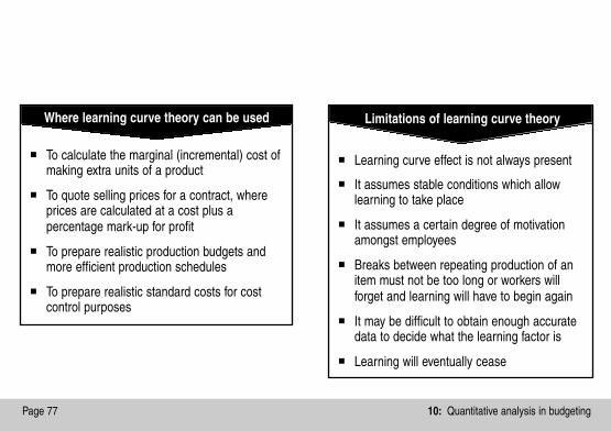
� To calculate the marginal (incremental) cost ofmaking extra units of a product
� To quote selling prices for a contract, whereprices are calculated at a cost plus apercentage mark-up for profit
� To prepare realistic production budgets andmore efficient production schedules
� To prepare realistic standard costs for costcontrol purposes
Where learning curve theory can be used
� Learning curve effect is not always present
� It assumes stable conditions which allowlearning to take place
� It assumes a certain degree of motivationamongst employees
� Breaks between repeating production of anitem must not be too long or workers willforget and learning will have to begin again
� It may be difficult to obtain enough accuratedata to decide what the learning factor is
� Learning will eventually cease
Limitations of learning curve theory
(010)ACF5PC_CH10.qxp 07/11/2010 00:59 Page 77

Forecasting techniques
Learningcurves
Expected valuesand spreadsheets
Analysing fixed andvariable costs
Expected values Spreadsheet packagescan be used in budgeting to determine the bestcombination of expected profit and risk.
are used to build business models and conduct‘what if’ analysis.
Assigns probabilities to different conditions
Probabilistic budgeting Disadvantages
A minor error in design can affect the validityof dataVery easy to corruptCan become over-dependent on them andlose sight of original intentionCannot take account of qualitative factors
�
��
�
Most likely Worst possible Best possible
Expected value of profits
���
(010)ACF5PC_CH10.qxp 07/11/2010 00:59 Page 78

11: Budgeting and standard costing
Topic List
Standard costs
Setting standards
Flexible budgets
This chapter revises standard costing and looks at howstandards are set.
Flexible budgets are vital for planning and control.
(011)ACF5PC_CH11.qxp 07/11/2010 01:00 Page 79
Standardcosts
Flexiblebudgets
Settingstandards
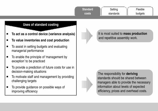
� To act as a control device (variance analysis)
� To value inventories and cost production
� To assist in setting budgets and evaluatingmanagerial performance
� To enable the principle of ‘management byexception’ to be practiced
� To provide a prediction of future costs for use indecision-making situations
� To motivate staff and management by providingchallenging targets
� To provide guidance on possible ways ofimproving efficiency
Uses of standard costing
It is most suited to mass productionand repetitive assembly work.
The responsibility for derivingstandards should be shared betweenmanagers able to provide the necessaryinformation about levels of expectedefficiency, prices and overhead costs.
(011)ACF5PC_CH11.qxp 07/11/2010 01:00 Page 80

Standardcosts
Flexiblebudgets
Settingstandards
11: Budgeting and standard costingPage 81
Ideal
� Perfect operating conditions� Unfavourable motivational impact
Attainable� Allowances made for inefficiencies and wastage� Incentive to work harder (realistic but challenging)
Current� Based on current working conditions� No motivational impact
Basic
� Unaltered over a long period of time� Unfavourable impact on performance
Types of performance standard Wastage
Build into an attainablematerials standard eg 20% normal loss 2kgx 100/80 = 2.5kg
Adjust materialsbudget
Idle time
Build into an attainablelabour hours standard
eg 20% idle time1hr x 100/80 = 1.25 hrs
Adjust labourbudget
(011)ACF5PC_CH11.qxp 07/11/2010 01:00 Page 81
Standardscosts
Setting standards
Flexiblebudgets
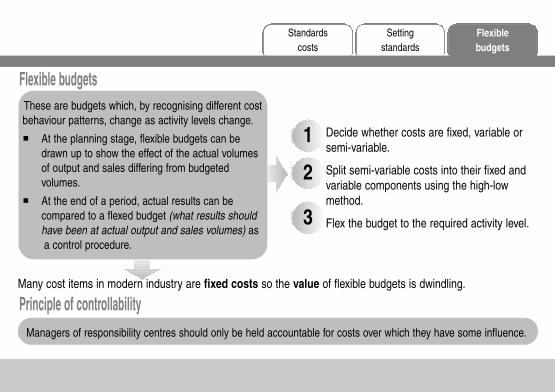
Flexible budgets
Decide whether costs are fixed, variable orsemi-variable.
Split semi-variable costs into their fixed andvariable components using the high-lowmethod.
Flex the budget to the required activity level.
2
3
1
These are budgets which, by recognising different costbehaviour patterns, change as activity levels change.
� At the planning stage, flexible budgets can bedrawn up to show the effect of the actual volumesof output and sales differing from budgetedvolumes.
� At the end of a period, actual results can becompared to a flexed budget (what results shouldhave been at actual output and sales volumes) asa control procedure.
Many cost items in modern industry are fixed costs so the value of flexible budgets is dwindling.
Principle of controllabilityManagers of responsibility centres should only be held accountable for costs over which they have some influence.
(011)ACF5PC_CH11.qxp 07/11/2010 01:00 Page 82

12: Variance analysis
Topic List
Basic variances
Idle time and waste
Operating statements
Investigating variances
Materials mix and yield variances
Sales mix and quantity variances
Variance analysis is a key technique in managementaccounting which you will have covered in your earlierstudies.
F5 will examine the more complicated variances such asmaterials mix and yield.
(012)ACF5PC_CH12.qxp 07/11/2010 01:13 Page 83
Basicvariances
Materials mix andyield variances
Sales mix andquantity variances
Investigating variances
Operatingstatements
Idle timeand waste
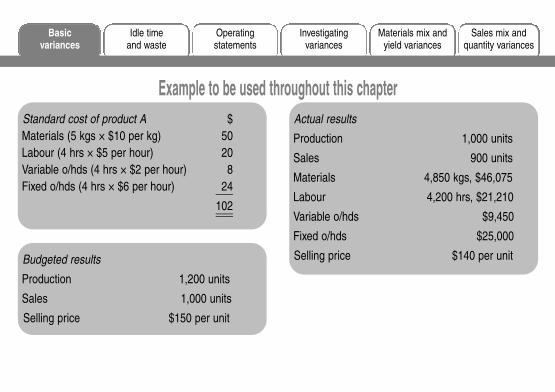
Example to be used throughout this chapterStandard cost of product A $Materials (5 kgs × $10 per kg) 50Labour (4 hrs × $5 per hour) 20Variable o/hds (4 hrs × $2 per hour) 8Fixed o/hds (4 hrs × $6 per hour) 24___
102______
Actual results
Production 1,000 units
Sales 900 units
Materials 4,850 kgs, $46,075
Labour 4,200 hrs, $21,210
Variable o/hds $9,450
Fixed o/hds $25,000
Selling price $140 per unitBudgeted results
Production 1,200 units
Sales 1,000 units
Selling price $150 per unit
(012)ACF5PC_CH12.qxp 07/11/2010 01:13 Page 84

Material total variance
Material price variance
Material usage variance
12: Variance analysisPage 85
Example$
1,000 units should have cost (× $50) 50,000but did cost 46,075______
Material total variance 3,925 (F)____________$
4,850 kgs should have cost (× $10) 48,500but did cost 46,075______
Material price variance 2,425 (F)____________
1,000 units should have used 5,000 kgsbut did use 4,850 kgs______
Variance in kgs 150 kgs (F)× standard cost per kg × $10______Material usage variance $1,500 (F)____________
The difference between what the output actually cost,and what it should have cost, in terms of material
This can be divided into two sub-variances.
The difference between the standard cost of thematerial that should have been used and the standardcost of the material that was used
The difference between what the material used didcost and what it should have cost
(012)ACF5PC_CH12.qxp 07/11/2010 01:13 Page 85
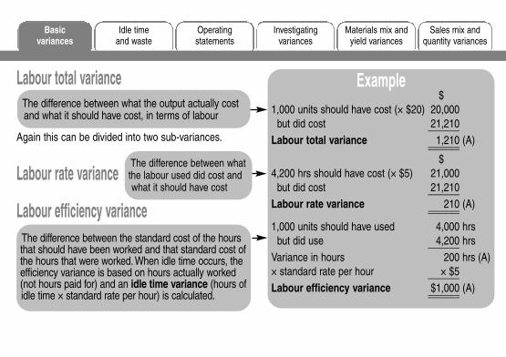
Example$
1,000 units should have cost (× $20) 20,000but did cost 21,210______
Labour total variance 1,210 (A)____________$
4,200 hrs should have cost (× $5) 21,000but did cost 21,210______
Labour rate variance 210 (A)____________
1,000 units should have used 4,000 hrsbut did use 4,200 hrs______
Variance in hours 200 hrs (A)× standard rate per hour × $5______Labour efficiency variance $1,000 (A)____________
Labour total varianceThe difference between what the output actually costand what it should have cost, in terms of labour
Again this can be divided into two sub-variances.
Labour rate varianceThe difference between whatthe labour used did cost andwhat it should have cost
The difference between the standard cost of the hoursthat should have been worked and that standard cost ofthe hours that were worked. When idle time occurs, theefficiency variance is based on hours actually worked(not hours paid for) and an idle time variance (hours ofidle time × standard rate per hour) is calculated.
Labour efficiency variance
Basicvariances
Materials mix andyield variances
Sales mix andquantity variances
Investigating variances
Operatingstatements
Idle timeand waste
(012)ACF5PC_CH12.qxp 07/11/2010 01:13 Page 86

12: Variance analysisPage 87
Example$
1,000 units should have cost (× $8) 8,000but did cost 9,450_____
Variable prod o/hd total variance 1,450 (A)__________
$4,200 hrs should have cost (× $2) 8,400
but did cost 9,450_____Variable prod o/hd exp’d variance 1,050 (A)__________
Labour efficiency variance in hrs 200 hrs (A)× standard rate per hour × $2_____Variable prod o/hd efficiency
variance $400 (A)__________
Variable production overhead total varianceThe difference between what the output should havecost and what it did cost, in terms of variableproduction overhead
Variable production o/hd expenditure varianceThe difference between the actual variable productionoverhead incurred and the amount that should havebeen incurred in the hours actively worked
Variable production o/hd efficiency varianceThe difference between the standard cost of thehours that should have been worked and the standardcost of the hours that were worked
(012)ACF5PC_CH12.qxp 07/11/2010 01:13 Page 87

The total variance is the difference between fixed production overhead incurred and fixed productionoverhead absorbed (= under- or over-absorbed fixed production overhead).
Example$
Actual prod’n at std rate(1,000 × $24) 24,000Budgeted prod’n at std rate(1,200 × $24) 28,800______Volume variance 4,800 (A)*____________
*(A) because actual output lessthan budgeted output
Example$
Overhead incurred 25,000Overhead absorbed(1,000 × $24) 24,000______Under-absorbedoverhead/totalvariance 1,000 (A)*____________
Example$
Budgeted o/hd (1,200 × $24) 28,800Actual overhead 25,000______Expenditure variance 3,800 (F)____________
Causes of under/over absorption� Actual expenditure ≠ budgeted
expenditure ⇒ expenditure variance
� Actual prod’n (units or hrs) ≠budgeted prod’n ⇒ volume variance
Expenditure varianceThe difference between budgetedand actual fixed productionoverhead expenditure
Basicvariances
Materials mix andyield variances
Sales mix andquantity variances
Investigating variances
Operatingstatements
Idle timeand waste
Volume varianceThe difference between actualand budgeted production units ×standard absorption rate per unit
(012)ACF5PC_CH12.qxp 07/11/2010 01:13 Page 88

12: Variance analysisPage 89
ExampleBudgeted hours (1,200 × 4) 4,800 hrsActual hours 4,200 hrs_____Variance in hrs 600 hrs(A)× std rate per hr × $6_____Capacity variance $3,600 (A)____________
ExampleLabour efficiency variance in hrs 200 hrs (A)× standard rate per hr × $6______Efficiency variance $1,200 (A)____________
Volume efficiency varianceShows how much of the under/over absorption is dueto efficiency of labour/plant
Volume capacity varianceShows how much of the under/over absorption is dueto hours worked being more or less than budgeted
The difference between the number ofhours that production should have takenand the number of hours worked ×standard absorption rate per hour
The difference between budgetedhours of work and actual hours worked× standard absorption rate per hour
This is usually the labourefficiency variance in hoursand so is also similar to the
variable productionoverhead efficiency
variance.
In a marginalcosting system there is
no volume variance.
(012)ACF5PC_CH12.qxp 07/11/2010 01:13 Page 89

Selling price varianceA measure of the effect on expected profit of adifferent selling price to standard
Sales volume varianceA measure of the effect on expected profitof a different sales volume to that budgeted
ExampleBudgeted sales volume 1,000 unitsActual sales volume 900 units____Variance in units 100 units(A)× std profit margin per unit(× $(150 – 102)) × $48____Sales volume variance $4,800 (A)____________
Example$
Revenue from 900 units should have been (× $150) 135,000
but was (× $140) 126,000______Selling price variance 9,000 (A)____________
The difference between the actual unitssold and the budgeted quantity, valued atthe standard profit per unit
The difference between what the salesrevenue should have been for the actualquantity sold, and what it was
Don’t forget to valuethe sales volume
variance at standardcontribution margin ifmarginal costing is in
use.
Basicvariances
Materials mix andyield variances
Sales mix andquantity variances
Investigating variances
Operatingstatements
Idle timeand waste
(012)ACF5PC_CH12.qxp 07/11/2010 01:13 Page 90

12: Variance analysisPage 91
Idle time variance Wastageis the number of hours that were idle, over andabove those expected, valued at the standard rateper hour.
Calculate a variance that compares actual materialusage with a standard that has been adjusted forexpected wastage.
ExampleBudgeted machine time = 5,000 hrs Excess idle time = 800 - (5% x 6,000) = 500Budgeted output = 18,525 units Budgeted cost of labour per hour = $44,460/5,000 x 100/95 = $9.36Idle time of 5% is allowed. Idle time variance = 500 x $9.36 = $4,680Total budgeted costs = $44,460Actual machine hours = 6,000Actual idle time = 800 hours
Basicvariances
Materials mix andyield variances
Sales mix andquantity variances
Investigating variances
Operatingstatements
Idle timeand waste
(012)ACF5PC_CH12.qxp 07/11/2010 01:13 Page 91

Most common presentation (marginal costing)$ $
Budgeted profit XBudgeted fixed production overhead X___Budgeted contribution XSales variances (price and volume) X___Actual sales minus std variable cost of sales XVariable cost variances X___Actual contribution XBudgeted fixed production overhead XExpenditure variance X__Actual fixed production overhead X
__Actual profit X______
Most common presentation (absorption costing)$ $
Budgeted profit XSales variances – price X
– volume X___X___
Actual sales minus standard cost of sales X
Cost variances $ $(F) (A)
Material price etc XFixed o/hd volume etc X___ ___
X X X___ ___ ___Actual profit X______
Within an ABC system efficiency variances for longer-term variable overheads are the difference between the levelof activity that should have been needed and the actual activity level, valued at the standard rate per activity.
Basicvariances
Materials mix andyield variances
Sales mix andquantity variances
Investigating variances
Operatingstatements
Idle timeand waste
(012)ACF5PC_CH12.qxp 07/11/2010 01:13 Page 92

12: Variance analysisPage 93
Material price (F) – unforeseen discounts received(A) – price increase, careless purchasing
Material usage (F) – material used higher quality thanstandard
(A) – defective material, waste, theftLabour rate (F) – use of less skilled (lower paid) workers
(A) – rate increaseIdle time (always (A)) – machine breakdown, illnessLabour efficiency (F) – better quality materials
(A) – lack of trainingOverhead expenditure (F) – cost savings
(A) – excessive use of servicesOverhead volume - production greater or less than
budgeted
Reasons for variances
� Materiality � Type of standard used� Controllability � Variance trend� Costs v benefits
� Interdependence (eg material price (F) andmaterial usage (A))
Factors affecting the significance ofvariances
� Efficient/inefficient operations� Measurement errors� Out of date standards� Random/chance fluctuations
Causes of variances
Basicvariances
Materials mix andyield variances
Sales mix andquantity variances
Investigating variances
Operatingstatements
Idle timeand waste
(012)ACF5PC_CH12.qxp 07/11/2010 01:13 Page 93

Rule of thumb methodDeciding a limit and if variance is within limit notinvestigated, if outside limit action is taken.
Statistical significance modelUse of historical data to calculate expected averageand standard deviation. Variance investigated only ifgreater distance from average than normaldistribution suggests is likely if process is in control.
� Limits set randomly
� Limits different for unfavourable
� Fixed percentage limits hide significantabsolute losses
� Unimportant/expected fluctuations highlightedunnecessarily
� Costs/benefits of investigations not highlighted
� Past history of variances ignored
Drawbacks of method
� Important costs with small variationshighlighted if variances rise significantly
� Costs with normal large variations nothighlighted unless variations excessive
BUT
How do you ascertain standard deviations ofexpenditure?
Advantages of method
Basicvariances
Materials mix andyield variances
Sales mix andquantity variances
Investigating variances
Operatingstatements
Idle timeand waste
(012)ACF5PC_CH12.qxp 07/11/2010 01:13 Page 94

12: Variance analysisPage 95
If a product requires two or more raw materials, and the proportions of the materials are changeable andcontrollable, the materials usage variance can be split into a mix variance and a yield variance.
Materials mix varianceA measure of whether the actual mix is cheaper ormore expensive that the standard and calculated asthe difference between the actual total quantityused in the standard mix and the actual quantityused in the actual mix, valued at standard costs.
� Find the standard proportions of the mix
� Calculate the standard mix of the actual material used
� Find (in kgs, litres etc for each input) the differencebetween what should have been used (as calculatedabove) and what was used
� Value at standard costs
ExampleMaterial A Material B
Mix should have been(say 600 kgs split 2:3) 240 kgs 360 kgsBut was (say) 250 kgs 350 kgs___ ___Mix variance in kgs 10 kgs (A) 10 kgs (F)× std cost per kg (say) × $10 × $5____ ____
$100 (A) $50 (F)____ ________ ____
The mix variance in quantity is always zero.
Basicvariances
Materials mix andyield variances
Sales mix andquantity variances
Investigating variances
Operatingstatements
Idle timeand waste
(012)ACF5PC_CH12.qxp 07/11/2010 01:13 Page 95

Materials yield variance in total Materials yield variance for individual materials
A BStd usage for actual output 260 kgs 390 kgsActual usage in std mix 240 kgs 360 kgs___ ___Yield variance in kgs 20 kgs(F) 30 kgs(F)× std cost per kg × $10 × $5____ ____Yield variance in $ $200 (F) $150 (F)____ ________ ____
� Arises because there is adifference between what theinputs should have been forthe output achieved and theactual inputs
� Calculated as the differencesbetween std inputs for actualoutput and std mix of actualtotal input, valued at std costs
ExampleStd input to produce 1 unit of X:A 20 kgs × $10 $200B 30 kgs × $5 $150__ ____
50 kgs $350__ ______ ____
In May, 13 units of X were producedfrom 250 kgs of A and 350 kgs of B.
� A measure of the effect oncosts of inputs yielding more orless than expected
� Calculated as the differencebetween the expected outputfrom the actual input and theactual output, valued at thestandard cost per unit of output
(250 + 350)kgs should have yielded (÷ 50kgs) 12Xbut did yield 13X__Yield variance in units 1X (F)× standard cost per unit of output × $350____Yield variance in $ $350 (F)________
Basicvariances
Materials mix andyield variances
Sales mix andquantity variances
Investigating variances
Operatingstatements
Idle timeand waste
(012)ACF5PC_CH12.qxp 07/11/2010 01:13 Page 96

� Occurs when the proportions of thevarious products sold are different fromthose in the budget.
� Shows the difference in contribution / profitbecause of a change in sales volume fromthe budgeted volume of sales.
12: Variance analysisPage 97
Basicvariances
Materials mix andyield variances
Sales mix andquantity variances
Investigating variances
Operatingstatements
Idle timeand waste
If a company sells more than one product, it is possible to analyse the overall sales volume variance into asales mix variance and a sales quantity variance.
Sales mix variance Sales quantity variance
Units
Actual sales (standard mix) XStandard sales (standard mix) XDifference XDifference × standard profit $X (A)/(F)
Units‘Should’ mix (actual quantity, standard mix) X‘Did’mix (actual quantity, actual mix) XDifference XDifference × standard margin $X (A)/(F)
(012)ACF5PC_CH12.qxp 07/11/2010 01:13 Page 97

Notes
(012)ACF5PC_CH12.qxp 07/11/2010 01:13 Page 98

13: Behavioural aspects of standard costing
Topic List
Planning and operational variances
Behavioural aspects
Standard costs and variances affect staff motivation andaction. Motivation will be improved if staff are only heldresponsible for controllable variances.
(013)ACF5PC_CH13.qxp 07/11/2010 01:16 Page 99

Behaviouralaspects
Planning andoperational variances
Arise because of inaccurateplanning/faulty standards and sonot controllable by operationalmanagers but by seniormanagementCalculated by comparing anoriginal standard with a revisedstandard
Caused by adverse/favourable operational performanceCalculated by comparing actual results with a realistic,revised standard/budget
Planning variances
Operational variances
� Highlight controllable anduncontrollable variances
� Increase both managers’acceptance of the use ofvariances for performancemeasurement and managers’motivation
� Improve planning andstandard-setting processes asstandards are more accurate,relevant and appropriate
� Operational variances providea fairer reflection of actualperformance
Advantages
� Difficulty in determiningrealistic standards
� Danger of managersattempting to explain allvariances as planning errors
� Time-consuming preparation
� Do not provide an overallpicture of the total variance
Disadvantages
(013)ACF5PC_CH13.qxp 07/11/2010 01:16 Page 100

13: Behavioural aspects of standard costingPage 101
Planning and operational variances
A revised budget can be calculated using revised standards so that only operational variances arehighlighted when actual results are compared to the revised budget.
Revised budget
Materials Labour Sales
Price Usage Rate Efficiency Revise the sales budget forchanges in market size, market
share, price, volume
(013)ACF5PC_CH13.qxp 07/11/2010 01:16 Page 101
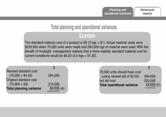
Total planning and operational variancesExample
The standard material cost of a product is $3 (3 kgs × $1). Actual material costs were$250,000 when 70,000 units were made and 200,000 kgs of material were used. With thebenefit of hindsight, management realises that a more realistic standard material cost forcurrent conditions would be $4.20 (3.5 kgs × $1.20).
$Revised standard cost
(70,000 × $4.20) 294,000Original standard cost
(70,000 × $3) 210,000_______Total planning variance 84,000 (A)______________
$70,000 units should have cost
(using revised std of $4.20) 294,000but did cost 250,000______Total operational variance 44,000 (F)____________
Behaviouralaspects
Planning andoperational variances
(013)ACF5PC_CH13.qxp 07/11/2010 01:16 Page 102
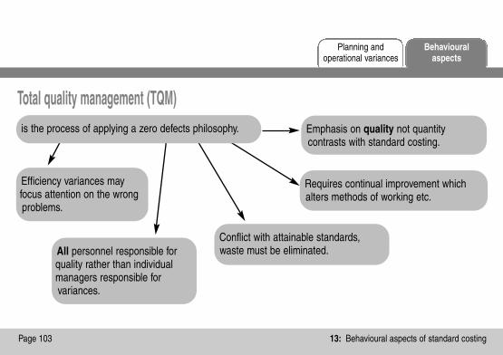
Behaviouralaspects
Planning andoperational variances
13: Behavioural aspects of standard costingPage 103
Total quality management (TQM)is the process of applying a zero defects philosophy. Emphasis on quality not quantity
contrasts with standard costing.
Requires continual improvement whichalters methods of working etc.
Efficiency variances mayfocus attention on the wrongproblems.
All personnel responsible forquality rather than individualmanagers responsible forvariances.
Conflict with attainable standards,waste must be eliminated.
(013)ACF5PC_CH13.qxp 07/11/2010 01:16 Page 103

Problems with standard costing
Why is it still used?
� Concentrates on a narrow range of costs
� Too much emphasis on direct labour costs andother short-term variable costs
� Relies on repetitive operation and homogenousoutput
� Business environment is increasingly dynamicand unstable
� Information produced is not sufficient timely
� Organisations still need to plan and quantifybudgets
� Cost and mix changes from plan still relevant
� Use standards as a starting point in costconstruction for a new product
� Used for product pricing
� Trends can be monitored over time
� Accounting valuations
Behaviouralaspects
Planning andoperational variances
(013)ACF5PC_CH13.qxp 07/11/2010 01:16 Page 104

14: Performance measurement
Topic List
Performance measurement
Balanced scorecard
Building Block model
Performance measurement aims to establish how wellsomething or someone is doing in relation to a plannedactivity. It is a vital part of the control process and can bedone using financial and non-financial performanceindicators. Remember that different performancemeasures are appropriate for different organisations.
(014)ACF5PC_CH14.qxp 07/11/2010 01:18 Page 105
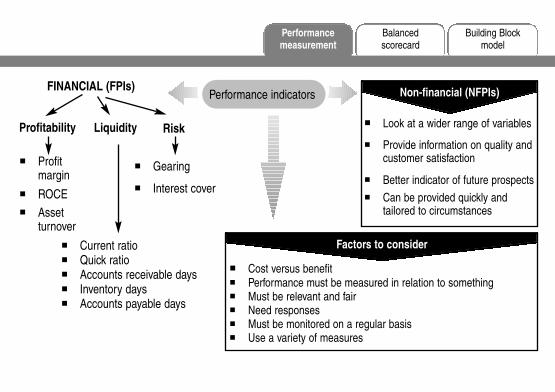
Building Block model
Balancedscorecard
Performancemeasurement
Non-financial (NFPIs)
� Look at a wider range of variables
� Provide information on quality andcustomer satisfaction
� Better indicator of future prospects
� Can be provided quickly andtailored to circumstances
Factors to consider
� Cost versus benefit� Performance must be measured in relation to something� Must be relevant and fair� Need responses� Must be monitored on a regular basis� Use a variety of measures
FINANCIAL (FPIs)
Profitability Liquidity Risk
� Profitmargin
� ROCE
� Assetturnover
� Current ratio� Quick ratio� Accounts receivable days� Inventory days� Accounts payable days
� Gearing
� Interest cover
Performance indicators
(014)ACF5PC_CH14.qxp 07/11/2010 01:18 Page 106
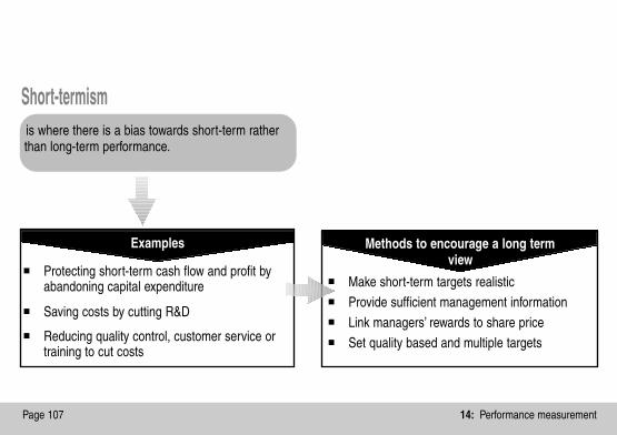
14: Performance measurementPage 107
Short-termism
Examples
is where there is a bias towards short-term ratherthan long-term performance.
� Protecting short-term cash flow and profit byabandoning capital expenditure
� Saving costs by cutting R&D
� Reducing quality control, customer service ortraining to cut costs
� Make short-term targets realistic
� Provide sufficient management information
� Link managers’ rewards to share price
� Set quality based and multiple targets
Methods to encourage a long termview
(014)ACF5PC_CH14.qxp 07/11/2010 01:18 Page 107

Building block model
Balancedscorecard
Performancemeasurement
Managers are required to focus on four different perspectives and use financial and non-financial indicators.
Perspective Question Explanation
Customer What do existing and new customersvalue from us?
Gives rise to targets that matter to customers: cost,quality, delivery, inspection, handling and so on.
Internal What processes must we excel at toachieve our financial and customerobjectives?
Aims to improve internal processes and decisionmaking.
Innovation andlearning
Can we continue to improve and createfuture value?
Considers the business's capacity to maintain itscompetitive position through the acquisition of newskills and the development of new products.
Financial How do we create value for ourshareholders?
Covers traditional measures such as growth,profitability and shareholder value but set throughtalking to the shareholder or shareholders direct.
(014)ACF5PC_CH14.qxp 07/11/2010 01:18 Page 108
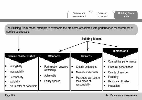
Building Block model
Balancedscorecard
Performancemeasurement
14: Performance measurementPage 109
Service characteristics
� Intangibility
� Inseparability
� Perishability
� Variability
� No transfer of ownership
Standards
� Participation ensuresownership
� Achievable
� Equity applies
Rewards
� Clearly understood
� Motivate individuals
� Managers can controltheir areas ofresponsibility
Dimensions
� Competitive performance
� Financial performance
� Quality of service
� Flexibility
� Resource utilisation
� Innovation
The Building Block model attempts to overcome the problems associated with performance measurement ofservice businesses.
Building Blocks
(014)ACF5PC_CH14.qxp 07/11/2010 01:18 Page 109

Notes
(014)ACF5PC_CH14.qxp 07/11/2010 01:18 Page 110

15: Divisional performance measures
Topic List
Divisionalisation
Performance measures
Transfer pricing
When organisations have a divisional structure, divisionalperformance measures will be required and transferpricing may be used.
(015)ACF5PC_CH15.qxp 07/11/2010 01:19 Page 111

Transferpricing
Performancemeasures
Divisionalisation
Dysfunctional decision making (abalance has to be kept betweendecentralisation of authority to provideincentives and motivation, andretaining centralised authority toensure goal congruence)Increase in costs of activities commonto all divisionsLoss of control by top management
It can improve the decision-making process in two ways– Quality– SpeedThe authority to act to improve performance shouldmotivate divisional managersTop management are freed from detailed involvement inday-to-day operations and can devote more time tostrategic planningDivisions provide valuable training grounds for futuremembers of top management
Disadvantages of divisionalisationAdvantages of divisionalisation
There are two common ways of structuring organisations. � Functionally� Divisionally
In general, a divisional structure will lead to decentralisation of the decision-making process.
� �
�
�
�
�
�
(015)ACF5PC_CH15.qxp 07/11/2010 01:19 Page 112

Transferpricing
Performancemeasures
Divisionalisation
15: Divisional performance measuresPage 113
Responsibility accountingis where authority is decentralised
TYPES OF RESPONSIBILITY CENTRE Cost centre Profit centre Investment centre
PRINCIPAL PERFORMANCE MEASURES� Variance analysis� Efficiency measures
� Profitability � Return on investment
� Residual income
(015)ACF5PC_CH15.qxp 07/11/2010 01:19 Page 113
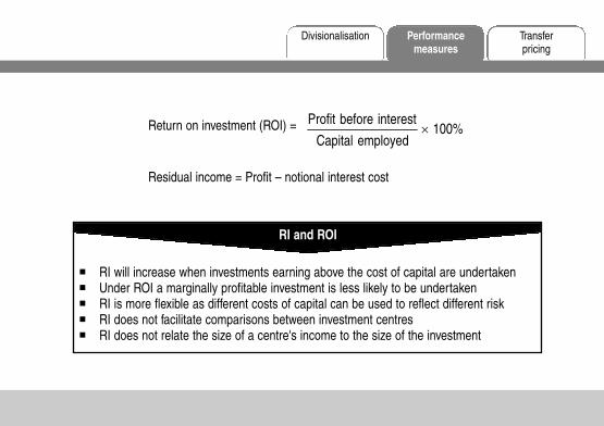
Transferpricing
Performancemeasures
Divisionalisation
Return on investment (ROI) = 100%employedCapital
interestbeforeProfit×
Residual income = Profit – notional interest cost
� RI will increase when investments earning above the cost of capital are undertaken� Under ROI a marginally profitable investment is less likely to be undertaken� RI is more flexible as different costs of capital can be used to reflect different risk� RI does not facilitate comparisons between investment centres� RI does not relate the size of a centre's income to the size of the investment
RI and ROI
(015)ACF5PC_CH15.qxp 07/11/2010 01:19 Page 114

Transferpricing
Performancemeasures
Divisionalisation
15: Divisional performance measuresPage 115
Transfer priceis the price at which goods and services aretransferred from one division to another.
MINIMUM MAXIMUM
Marginal cost plus opportunitycost of item transferred
Lowest external market priceminus internal cost saving on packagingand delivery
Opportunity cost is the maximumcontribution foregone by transferringinternally
� Promotedivisionalautonomy
� Equitabledivisionalperformancemeasurement
� Overallcorporate profitmaximisation
Aims
Market price may be temporaryDisincentive to use up spare capacityNo market price availableImperfect external market
Disadvantages
�
���
(015)ACF5PC_CH15.qxp 07/11/2010 01:19 Page 115

Transfer prices based on costIf there is no external market, the transfer price has to be based on cost.
Standard or actual? The use of standard costs is fairer because if actual costs are used thetransferring division has no incentive to control its costs – it can pass on itsinefficiencies to the receiving division.
Variable cost? The transferring division does not cover its fixed costs (although this problemcan be overcome by central decisions or by some form of dual pricing or two-part charging system).
Full cost? The transferring division makes no profit.
Full cost plus? What margin will all parties perceive as fair?
1
4
3
2
Optimal transfer price
Transferpricing
Performancemeasures
Divisionalisation
reflects opportunity costs and where there is a perfect external market this will be the market price. If not, theideal transfer price will be found by negotiation and careful analysis.
(015)ACF5PC_CH15.qxp 07/11/2010 01:19 Page 116

16: Further performance management
Topic List
Not-for-profit organisations
External considerations
Behaviour aspects
Not-for-profit organisations and the public sector havenon-quantifiable and multiple objectives which causesproblems in performance measurement.
Organisations must also consider external influences onperformance.
(016)ACF5PC_CH16.qxp 07/11/2010 01:22 Page 117

Behaviouraspects
Externalconsiderations
Not-for-profitorganisations
Not-for-profit organisationshave a range of multiple objectives which aredifficult to define.
Value for money
Problem with performance measurement
Solutions
� Efficiency: Relationship between inputs andoutputs (getting out as much as possible forwhat goes in)
� Effectiveness: Relationship between outputsand objectives (getting done what wassupposed to be done)
� Economy: Obtaining the right quality andquantity of inputs at lowest cost (being frugal)
� Multiple objectives� Measuring outputs� Lack of profit measure� Nature of service provided� Financial constraints� Political, social and legal considerations
� Judge performance in terms of inputs� Use experts’ subjective judgement� Use benchmarking� Use unit cost quantitative measures
(016)ACF5PC_CH16.qxp 07/11/2010 01:22 Page 118

Behaviouraspects
Externalconsiderations
Not-for-profitorganisations
16: Further performance managementPage 119
Performance measurement needs to allow for external considerations.
Stakeholders
Internal Connected External
Employees Shareholders GovernmentCustomers
Moraleindex
Share priceWarranty cost% of repeat customers
% of productsconforming toenvironmental regulations
� Economic growth� Local economic trends� Inflation� Interest rates� Exchange rates� Government fisal policy� Government spending
Market conditions
� Pricing strategies� Information on
competitors’ prices andcost structures
� React quickly tochanging marketconditions
Competitors
(016)ACF5PC_CH16.qxp 07/11/2010 01:22 Page 119

Behaviouraspects
Externalconsiderations
Not-for-profitorganisations
Management performance measures should only include those items that are directly controllable by themanager.
Conflict between individualand corporate goals.
Reward schemes canencourage dysfunctional
behaviour.Danger people will
concentrate only on whatis being measured.
Difficult to devise performancemeasures relating specifically
to a manager’s performance asa manager.
(016)ACF5PC_CH16.qxp 07/11/2010 01:22 Page 120

Notes
(016)ACF5PC_CH16.qxp 07/11/2010 01:22 Page 121

Notes
(016)ACF5PC_CH16.qxp 07/11/2010 01:22 Page 122

(016)ACF5PC_CH16.qxp 07/11/2010 01:22 Page 123

Notes
(016)ACF5PC_CH16.qxp 07/11/2010 01:22 Page 124


![BPP - F7 INT Passcards[1]-2011](https://img.pdfslide.net/doc/110x75/544b14d5b1af9f7c4f8b4e32/bpp-f7-int-passcards1-2011.jpg)