Embed Size (px)
Citation preview
1
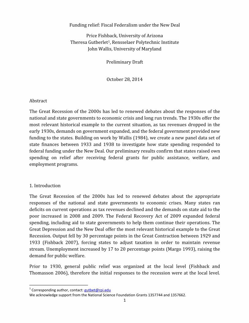
Funding relief: Fiscal Federalism under the New Deal
Price Fishback, University of Arizona
Theresa Gutberlet1, Rensselaer Polytechnic Institute
John Wallis, University of Maryland
Preliminary Draft
October 28, 2014
Abstract
The Great Recession of the 2000s has led to renewed debates about the responses of the
national and state governments to economic crisis and long run trends. The 1930s offer the
most relevant historical example to the current situation, as tax revenues dropped in the
early 1930s, demands on government expanded, and the federal government provided new
funding to the states. Building on work by Wallis (1984), we create a new panel data set of
state finances between 1933 and 1938 to investigate how state spending responded to
federal funding under the New Deal. Our preliminary results confirm that states raised own
spending on relief after receiving federal grants for public assistance, welfare, and
employment programs.
1. Introduction
The Great Recession of the 2000s has led to renewed debates about the appropriate
responses of the national and state governments to economic crises. Many states ran
deficits on current operations as tax revenues declined and the demands on state aid to the
poor increased in 2008 and 2009. The Federal Recovery Act of 2009 expanded federal
spending, including aid to state governments to help them continue their operations. The
Great Depression and the New Deal offer the most relevant historical example to the Great
Recession. Output fell by 30 percentage points in the Great Contraction between 1929 and
1933 (Fishback 2007), forcing states to adjust taxation in order to maintain revenue
stream. Unemployment increased by 17 to 20 percentage points (Margo 1993), raising the
demand for public welfare.
Prior to 1930, general public relief was organized at the local level (Fishback and
Thomasson 2006), therefore the initial responses to the recession were at the local level.
1 Corresponding author, contact: [email protected]
We acknowledge support from the National Science Foundation Grants 1357744 and 1357662.
2
For example, cities in Ohio used their local shares from property taxes to hand out direct
relief and to establish work-relief programs starting in 1929 (Maurer 1975). The state of
Ohio assumed fiscal responsibility for the relief effort in 1932, when it established the Ohio
State Relief Commission to provide funding for direct relief and public works (Dorn 1992).
States also offered loans to local governments to support ongoing expenditures. For
example, Massachusetts created the Emergency Municipal Finance Board in 1933, which
supervised the provision of $ 30 Million to local communities in its first year.2
The states had to find ways to fund their new fiscal responsibilities when their own
revenue streams were suffering from the economic contraction. Many did this by adding
new taxes. Between 1930 and 1940, the number of states with income taxes rose from 16
to 36 and 24 states introduced a general.3 The federal repeal of prohibition in 1933 made it
possible to levy sales and license taxes on alcoholic beverages, which were collected all 51
states by 1940. States with income taxes reduced exemptions and increased tax rates
during the 1930s. For example, Maryland began to tax personal incomes in 1937 at the rate
of 0.5 percent with an exemption of $2,500 for married couples. In 1939, the rate was
increased to 2.5 percent and the exemption was lowered to $2,000.4
The federal government began to provide funding in the form of matching grants and loans
for relief and recovery in 1932 under President Hoover. Federal funding for highway
construction supported the states’ relief efforts by reducing unemployment, but states
were obligated to raise a share of construction costs under the matching rules in the
Highway Act of 1916 (Fishback 2010). Federal grants to states for relief became available
for the first time under the New Deal. The Federal Emergency Relief Administration
(FERA), Works Progress Administration (WPA), Civil Works Administration (CWA), Civilian
Conservation Corps (CCC), Public Works Administration (WPA), and the Social Security Act
provided funds for direct transfers or work relief projects.
The statutes of most New Deal programs include matching provisions, requiring that states
raise their own funds to cover a share of relief spending. However, congressional and
administrative documents suggest that the matching provisions were enforced unequally
across states (Fishback and Wallis 2013). For example, Alabama state and local
governments provided six percent of the funds for FERA programs, while California
governments funded 30 percent of FERA spending (FERA 1937). The PWA had a mandate
to fund no more than 30 percent of specific project costs, but states could receive loans to
cover a large share of the remaining costs. The only agency that appears to have enforced
the statutory matching rates for its programs is the Social Security Administration, which
provided funds for public assistance programs after 1935.
2 The Boston Globe 24 February 1933
3 Financial Statistics of States 1930 and 1940
4 State of Maryland, Special Session April - May 1937, Chapter 11, Session Laws, Vol. 417, p. 22 ff. and Regular
Session January - April 1939, Chapter 277, Session Laws, Vol. 581, p. 468 ff.
3
2. Empirical Analysis
Our empirical analysis investigates how state spending on relief responded to federal
funding opportunities under the New Deal. On the one hand, the matching provisions of the
New Deal programs indicate that the states had to finance a share of relief and recovery
expenditures with own funds. In other words, state spending on public assistance and
welfare services should have increased in states that received federal grants for relief
programs. On the other hand, the evidence from New Deal program reports suggests that
the matching provisions were not applied equally across states and may not have been
enforced at all. Furthermore, states that took over fiscal responsibility for charitable
expenditures from local governments in the early 1930s could have replaced state level
relief with participation in the New Deal. In this case, federal spending on relief could have
provided a substitute for state spending.
We build on the empirical approach in Wallis (1984) to test whether federal relief spending
acted as a complement or substitute to state spending. Our panel data set allows us to add
fixed effects to the regression.
𝑅𝑒𝑙𝑖𝑒𝑓𝑖𝑡 = 𝛽1 𝐺𝑟𝑎𝑛𝑡𝑠𝑖𝑡 + 𝛽2 𝐼𝑛𝑐𝑜𝑚𝑒𝑖𝑡 + 𝛽3 𝐸𝑚𝑝𝑙𝑜𝑦𝑚𝑒𝑛𝑡𝑖𝑡 + 𝛽4 𝑆𝑡𝑎𝑡𝑒𝑖 + 𝛽5 𝑌𝑒𝑎𝑟𝑡 + 𝜀𝑖𝑡
In the regression equation, Reliefit measures total per capita spending on relief by state i in
year t, which includes current expenditures for care in state institutions, grants to private
charitable organizations, payments for public assistance and child welfare, and
expenditures for unemployment relief and employment services. To identify each state’s
own spending on relief, we subtract its current receipts from relief related federal grants.
State i’s revenue from federal grants enter our regression equation as the main variable of
interest Grantsit on the right hand side. We are interested in the sign of β1, which indicates
whether federal and state relief were complements (β1 > 0) or substitutes (β1 < 0).
We include Incomeit and Employmentit to control for the demand for public relief as well as
the states’ ability to raise revenue. Incomeit is composed of two variables, per capita
automobile and truck registrations in state i in year t and per capita income based on
estimates of total income in state i in year t. Vehicle registrations serve as a proxy for the
median income level, which may be a more relevant measure of the need for public
assistance than average income. Employmentit measures the level of employment, using an
index that compares the employment level in state i in year t to the level of employment in
the state in 1929. The control variables are taken from Finally, Statei and Yeart are sets of
state and year fixed effects. Our information about state relief expenditures and grant
receipts comes from state financial reports, which are difficult to read and differ greatly in
their content and format across states. Therefore, we use state fixed effects to limit
measurement error in our variables of interest. We assume that the unobserved factors
influencing state relief spending εit are uncorrelated with the observed right hand side
factors.
4
3. Sources and Construction of State Panel Data
Data on state finances has been collected and published by the U.S. Census Bureau since
1915 in an annual series entitled “Financial Statistics of States”.5 However, the publication
was interrupted from 1932 to 1936, leaving a large data gap when many New Deal
programs came into effect. In order to fill this gap, we have collected annual financial
reports by state comptrollers, state auditors, and treasury departments between 1930 and
1940. The state reports list receipts into revenue funds and disbursements made from
these funds, but often the line items do not match the categories used by the U.S. Census
Bureau. Furthermore, states administered multiple general, special, sinking, trust, and
investment funds, often making it unclear whether receipts into and disbursements from
individual funds reflect current revenues and cost payments or transfers across funds.
We have collected additional sources to help us match the state reports to the “Financial
Statistics of States”. To our knowledge, the U.S. Census Bureau published only one summary
of instructions for the compilation of the 1930s “Financial Statistics of States”.6 The small
booklet includes general descriptions of the U.S. Census Bureau’s revenue and cost
payments categories as well as special inquiries that census employees were to make about
specific budget items and funds. In addition, we have collected tax commission reports that
explain the allocation of tax revenues into specific funds, helping us to distinguish between
revenues and internal transfers. Finally, we have used the appropriation acts passed by
state legislatures to find more information about the purposes of particular disbursements.
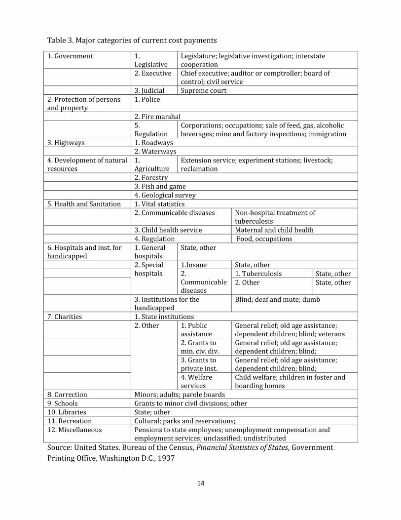
We use these sources to create a panel data set of state finances, adopting the current
revenue and current cost payments categories used in the “Financial Statistics of States”,
which are shown in Tables 2 and 3 in the appendix. Our panel currently covers 18 states
across all four census regions of the United States including Connecticut, Rhode Island, New
Hampshire, Pennsylvania, and Maryland in the Northeast, Virginia, Louisiana, Oklahoma,
and South Carolina in the South, Michigan, Minnesota, Nebraska, and Ohio in the Midwest,
and California, Colorado, New Mexico, Utah, and Washington in the West. The complexity of
state funds has forced us to abandon our original goal of matching the state financial
reports to the “Financial Statistics of States” by using just one or two years of overlapping
data. As a result, our panel currently includes revenue receipts and cost payments from
1933 to 1938, using only information from state reports.
3.1 Current Revenue Receipts
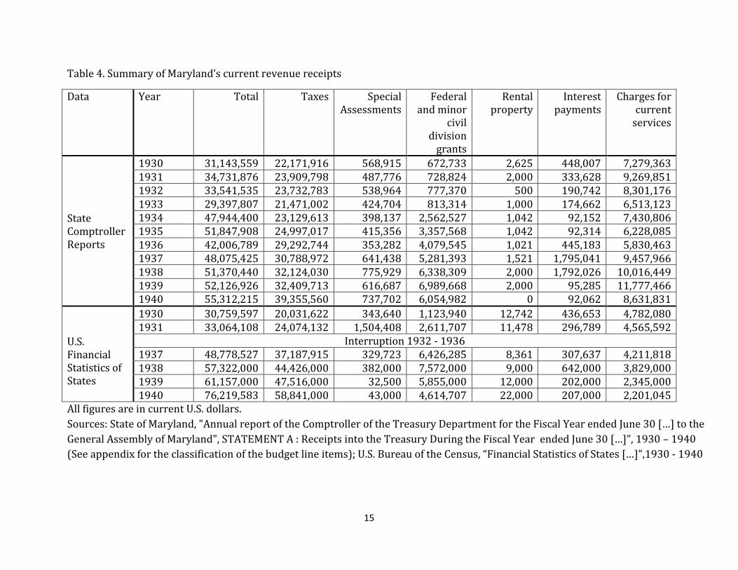
Maryland’s finances serve as an example to explain the construction of our panel data set.
Table 3 presents our summary of Maryland’s current revenue receipts based on the state
5 United States. Bureau of the Census, Financial Statistics of States, Government Printing Office, Washington D.C., 1915 -
6 United States. Bureau of the Census, Financial Statistics of States: Instructions to Clerks and Special Agents,
Government Printing Office, Washington D.C., 1928
5
comptroller reports and the U.S. Census Bureau’s account from the “Financial Statistics of
States”. According to our reading of the comptroller reports, Maryland’s total 1930 revenue
was $31,143,559, which is only $15,841 smaller than the census’ figure of $31,159,400.
However, our total revenues for 1938 to 1940 are substantially smaller than the numbers
provided in the “Financial Statistics of States” with the largest difference equal to
$20,907,368 in 1940.
The likeliest reason for this discrepancy lies in the structure of Maryland’s special revenue
funds. In the comptroller reports, receipts into special funds are often aggregated at the
fund level, for example the section “Sundry Funds Income” includes the line item “State
Accident Fund”. Maryland’s session laws of 1914 explain the revenue source for this
particular fund.
“Ten per centum of the premiums collected from employers insured in the State
Accident Fund shall be set aside by the Commissioners of the State Accident Fund
for the creation of a surplus […]”.7
The act indicates that Maryland used the “State Accident Fund” to collect insurance
premiums, which are nonrevenue receipts because they increase the state’s assets but also
raise its liabilities.8
A comparison of the top and bottom sections of Table 4 shows that the largest discrepancy
between our revenue account and the “Financial Statistics of States” arises in the
classification of tax revenues. For the years 1937 to 1940, our account of Maryland’s total
tax revenue is substantially lower than that of the U.S. Census Bureau, the largest difference
is equal to $19,485,440 in 1940. A possible reason for this discrepancy is that some tax
receipts were earmarked for debt service and booked into special funds, where they cannot
easily be recognized. The following section presents our data on tax revenues in more
detail to show what we can learn from the comptroller reports despite this challenge.
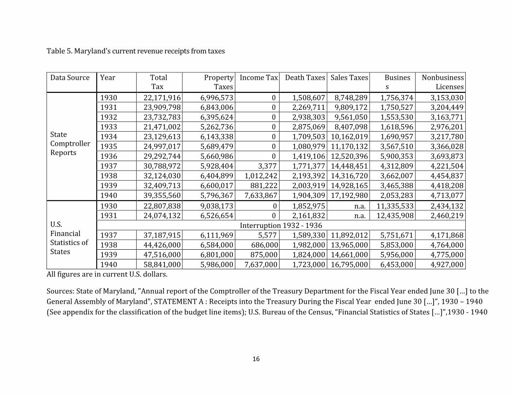
We have a detailed account of Maryland’s taxes at the beginning of the 1930s, because the
state revised its tax laws in 1929.9 Table 5 presents our account Maryland’s major tax
revenues compared to the figures provided by the U.S. Census Bureau. Although our total
tax revenue is significantly lower than the census’ for 1937 to 1940, the two series match
very closely for most important tax categories. In particular, the largest discrepancies for
property, income, and sales taxes between the two series are equal to $189,633 for
property taxes in 1940, $62,222 for income taxes in 1939, and $2,556,439 for sales taxes in
1937.
7 State of Maryland, Regular Session Jan - April 1914, Session Laws, Chapter 800, Section 23, p. 1441f.
8 United States. Bureau of the Census, Financial Statistics of States: Instructions to Clerks and Special Agents,
Government Printing Office, Washington D.C., 1928, p.8 9 State of Maryland, Regular Session January – April 1929, Chapter 226, Session Laws, Vol. 572, p. 621ff
6
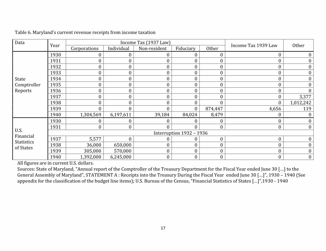
Maryland introduced its first state income tax at a rate of 0.5% on all corporate and
individual incomes with exemptions of $1,000 for individuals, $2,500 for married couples,
and $400 for each dependent in 1937.10 According to the state comptroller reports, the
initial revenue was equal to $3,377 in the fiscal year ending in 1937 and reached
$1,012,242 in the fiscal year ending in 1938. The income tax was amended in 1939, raising
the levy to 1.5% for corporations, 6% for individual investment income, and 2.5% for
individual wage income with a smaller exemption of only $2,000 for married couples.11 The
top of Table 6 shows that the revenue from the amended income tax was $7,633,687 or
19.4% of Maryland’s tax revenue by 1940. This figure is closely matched by the $7,637,000
in the “Financial Statistics of States” in the same table.
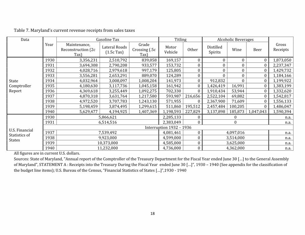
Prior to 1937, the “Financial Statistics of States” do not include a category for sales taxes,
therefore we cannot compare this figure directly to the census’ account. Earlier volumes
include the categories “Gasoline Tax” and “Motor Vehicle Titling Tax” in “Business License
Taxes”, which we show in Table 6. Maryland began to tax fuel purchases in 1922 at the rate
of $0.01 per gallon, increasing the rate to $0.04 in 1927 and $0.05 in 1947.12 The first
motor vehicle titling tax with a rate of 1 % of “…fair market value of every motor vehicle for
which an original certificate of title [is issued]” appears in Maryland’s session laws of
1936.13 Table 7 shows that revenue from automobile titling appears regularly in the state
comptroller reports from 1930 onward, but it does not increase significantly until 1936,
when it jumps from $161,942 to $702,330.
3.2 Current Cost Payments
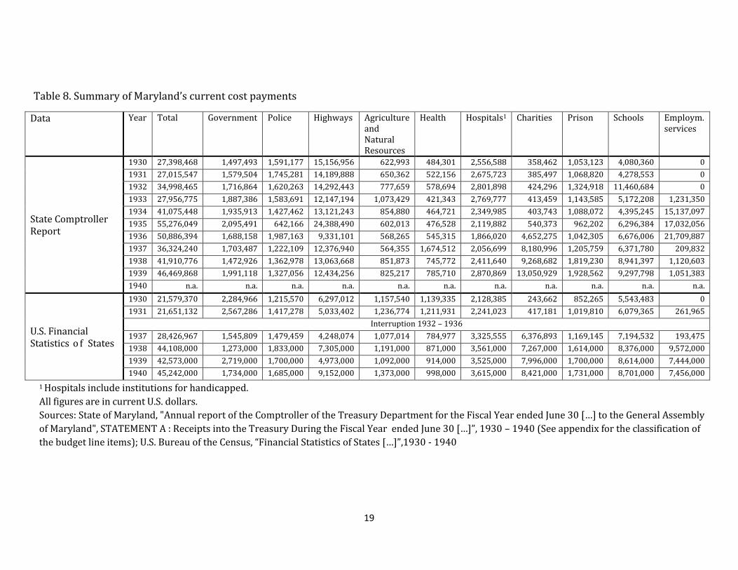
Maryland’s total cost payments increased from $27,398,468 in 1930 to $46,469,868 in
1939 according to our reading of the state comptroller reports. The “Financial Statistics of
States” report lower levels but a similar increase from $21,579,370 to $42,573,000. Table 8
shows that the sharpest rise in total cost payments from $27,956,775 in 1933 to
$41,075,448 in 1934 is due to spending on employment services. Generally, state
government expenditures do not rise dramatically from one year to the next, because new
spending has to be matched by new revenue. However, according to the 1934 comptroller
report, all spending on employment services in the fiscal year ending in 1934 was paid
from the “Unemployment Relief Federal Fund”, indicating that it was financed through
federal grants.
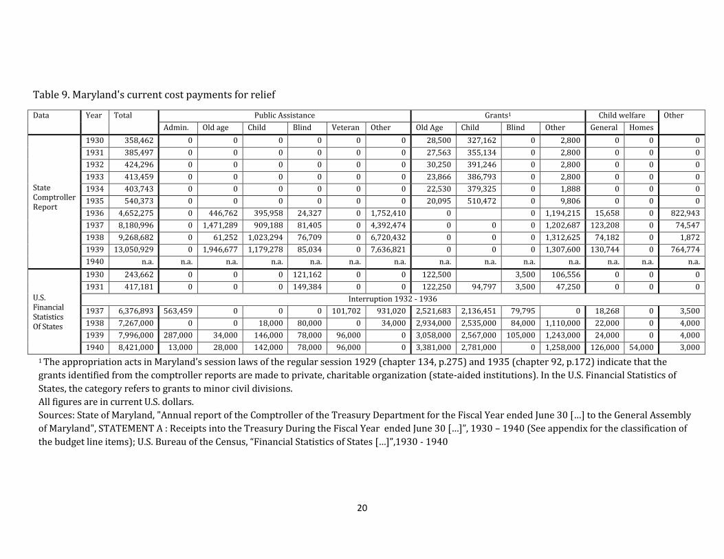
Maryland’s spending in the category “Charity” shifted away from state grants to private
charitable institutions in the early 1930s to spending on public assistance under the New
Deal. Table 9 shows our breakdown into spending on public assistance, grants, and welfare
services. Prior to 1936, almost all spending on charity in the comptroller reports was paid
10
State of Maryland, Special Session April - May 1937, Chapter 11, Session Laws, Vol. 417, p. 22 ff. 11
State of Maryland, Regular Session January - April 1939, Chapter 277, Session Laws, Vol. 581, p. 468 ff. 12
Maryland’s Revenue Structure, p.170 ff. 13
State of Maryland, Regular Session January - April 1936, Chapter 3, Session Laws, Vol. 577, p. 5 ff.
7
to private institutions in the form of grants.14 The state’s sole direct expenditure was for
supervision through the “Board of State Aid and Charities”. From 1936 onward, the
comptroller reports include aggregate payments to “State Aided Institutions”, which are
equal to $1,194,215 in 1936 and rise only slightly to $1,307,600 in 1939. These aggregates
match the U.S. Census Bureau’s figures in the subcategory “Other” in “Grants to Minor Civil
Divisions”, indicating that the census included grants to private institutions here.
Starting in 1936, the comptroller reports list disbursements from federal and other trust
funds with titles like “Old Age Assistance Federal Fund” and “Public Assistance Fund for Aid
to the Needy Blind”. We categorize these disbursements under “Public Assistance” in Table
9, which shows that they are much larger than the corresponding figures in the “Financial
Statistics of States”. The differences are explained by the census’ separation of spending
into “Public Assistance” and “Grants to Minor Civil Division”, which together add up to total
spending in “Public Assistance” according to the state comptroller reports. In this regard,
our panel cannot provide the same distinction between government spending at the state
and local level as the “Financial Statistics of States”.
4. Results
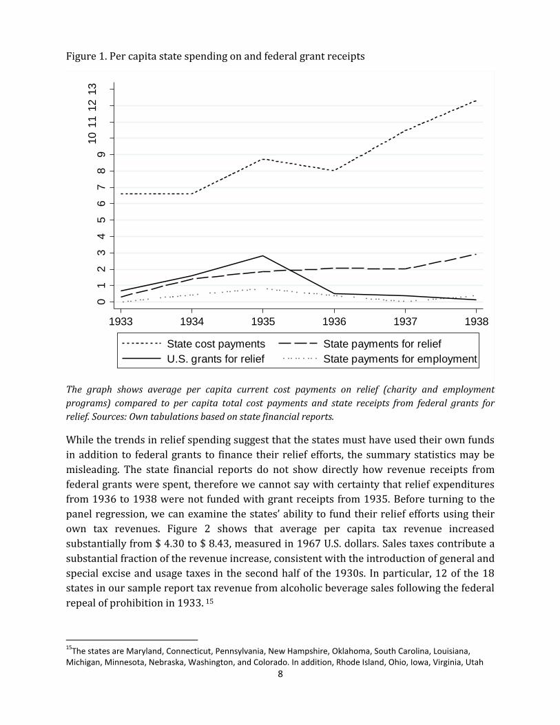
Our panel shows substantial increases in state expenditures and revenues between 1933
and 1938, consistent with the expansion of fiscal responsibility at the state level and the
introduction of new taxes to finance the spending increases. In particular, average per
capita spending on relief rose from $ 0.31 in 1933 to $ 2.91 in 1938, measured in 1967 U.S.
dollars. Figure 1 shows that half of the initial large increase in average relief expenditures
in 1934 and 1935 was due to spending on unemployment relief and employment services.
From 1936 onward, spending on charity, which includes public assistance and welfare
services, constitutes almost all of the states’ overall relief effort.
In our panel, per capita state revenue receipts from relief related federal grants also
reached their highest level of $ 2.85 in 1935, surpassing the average level of state relief
spending. The concurrent rise in federal grant receipts and state spending suggests that
states financed their relief efforts entirely by using federal funding. However, from 1936 to
1938, average state spending on relief continued to increase, while the states’ receipts from
federal grants for charity and employment programs decreased significantly. By 1938, the
average state in our panel spent approximately one quarter of total current cost payments
on relief related programs and received less than 5 percent of this spending in relief related
grants from the federal government.
14
Before 1936 the comptroller reports list each institution that received moneys from the state as an individual line item. We categorize these institutions as providing aid to the elderly, children, blind, or other groups based on their names and confirm that they are private by checking that they are listed as state aided institutions in the appropriation acts in Maryland’s session laws.
8
Figure 1. Per capita state spending on and federal grant receipts
The graph shows average per capita current cost payments on relief (charity and employment
programs) compared to per capita total cost payments and state receipts from federal grants for
relief. Sources: Own tabulations based on state financial reports.
While the trends in relief spending suggest that the states must have used their own funds
in addition to federal grants to finance their relief efforts, the summary statistics may be
misleading. The state financial reports do not show directly how revenue receipts from
federal grants were spent, therefore we cannot say with certainty that relief expenditures
from 1936 to 1938 were not funded with grant receipts from 1935. Before turning to the
panel regression, we can examine the states’ ability to fund their relief efforts using their
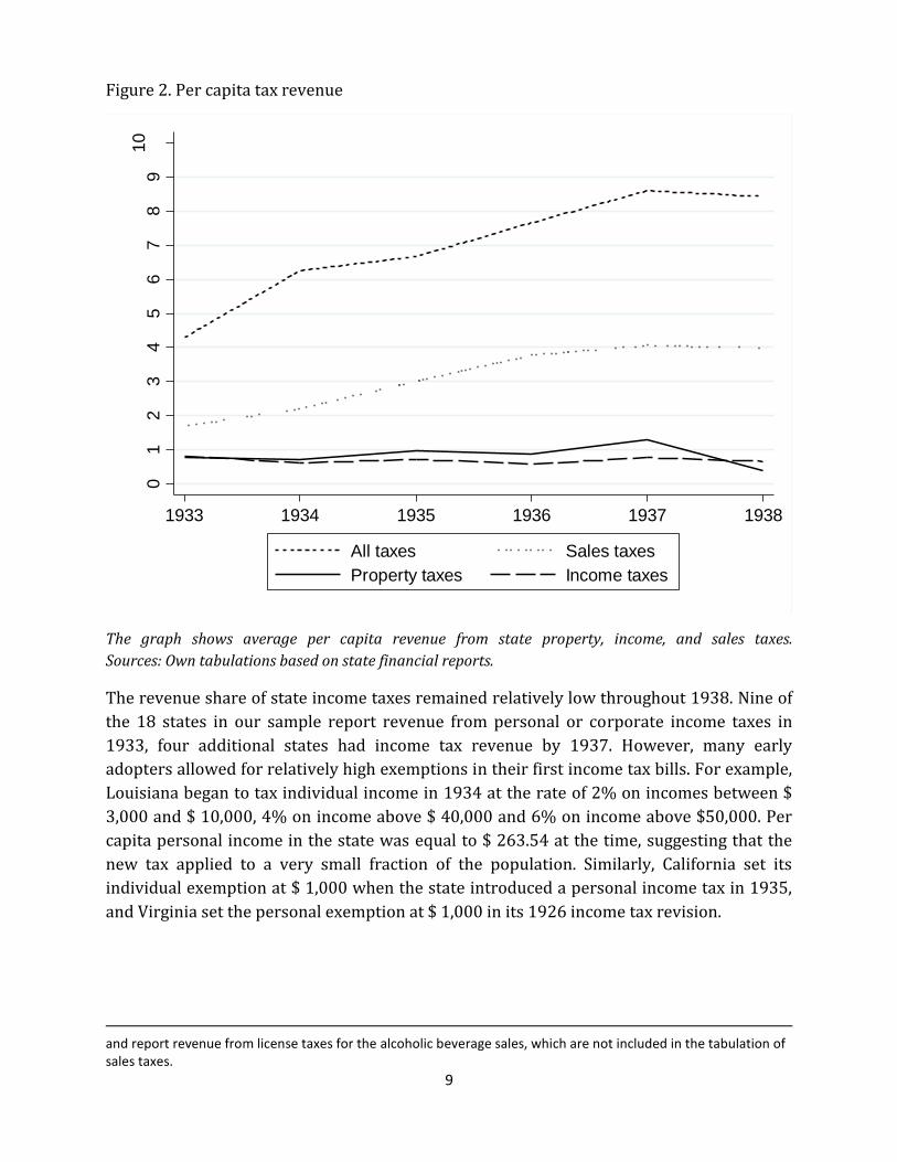
own tax revenues. Figure 2 shows that average per capita tax revenue increased
substantially from $ 4.30 to $ 8.43, measured in 1967 U.S. dollars. Sales taxes contribute a
substantial fraction of the revenue increase, consistent with the introduction of general and
special excise and usage taxes in the second half of the 1930s. In particular, 12 of the 18
states in our sample report tax revenue from alcoholic beverage sales following the federal
repeal of prohibition in 1933. 15
15
The states are Maryland, Connecticut, Pennsylvania, New Hampshire, Oklahoma, South Carolina, Louisiana, Michigan, Minnesota, Nebraska, Washington, and Colorado. In addition, Rhode Island, Ohio, Iowa, Virginia, Utah
01
23
45
67
89
10
11
12
13
1967 U
.S. dolla
rs
1933 1934 1935 1936 1937 1938
State cost payments
U.S. grants for relief
State payments for relief
State payments for employment
9
Figure 2. Per capita tax revenue
The graph shows average per capita revenue from state property, income, and sales taxes.
Sources: Own tabulations based on state financial reports.
The revenue share of state income taxes remained relatively low throughout 1938. Nine of
the 18 states in our sample report revenue from personal or corporate income taxes in
1933, four additional states had income tax revenue by 1937. However, many early
adopters allowed for relatively high exemptions in their first income tax bills. For example,
Louisiana began to tax individual income in 1934 at the rate of 2% on incomes between $
3,000 and $ 10,000, 4% on income above $ 40,000 and 6% on income above $50,000. Per
capita personal income in the state was equal to $ 263.54 at the time, suggesting that the
new tax applied to a very small fraction of the population. Similarly, California set its
individual exemption at $ 1,000 when the state introduced a personal income tax in 1935,
and Virginia set the personal exemption at $ 1,000 in its 1926 income tax revision.
and report revenue from license taxes for the alcoholic beverage sales, which are not included in the tabulation of sales taxes.
01
23
45
67
89
10
1967 U
.S. dolla
rs
1933 1934 1935 1936 1937 1938
All taxes Sales taxes
Property taxes Income taxes
10
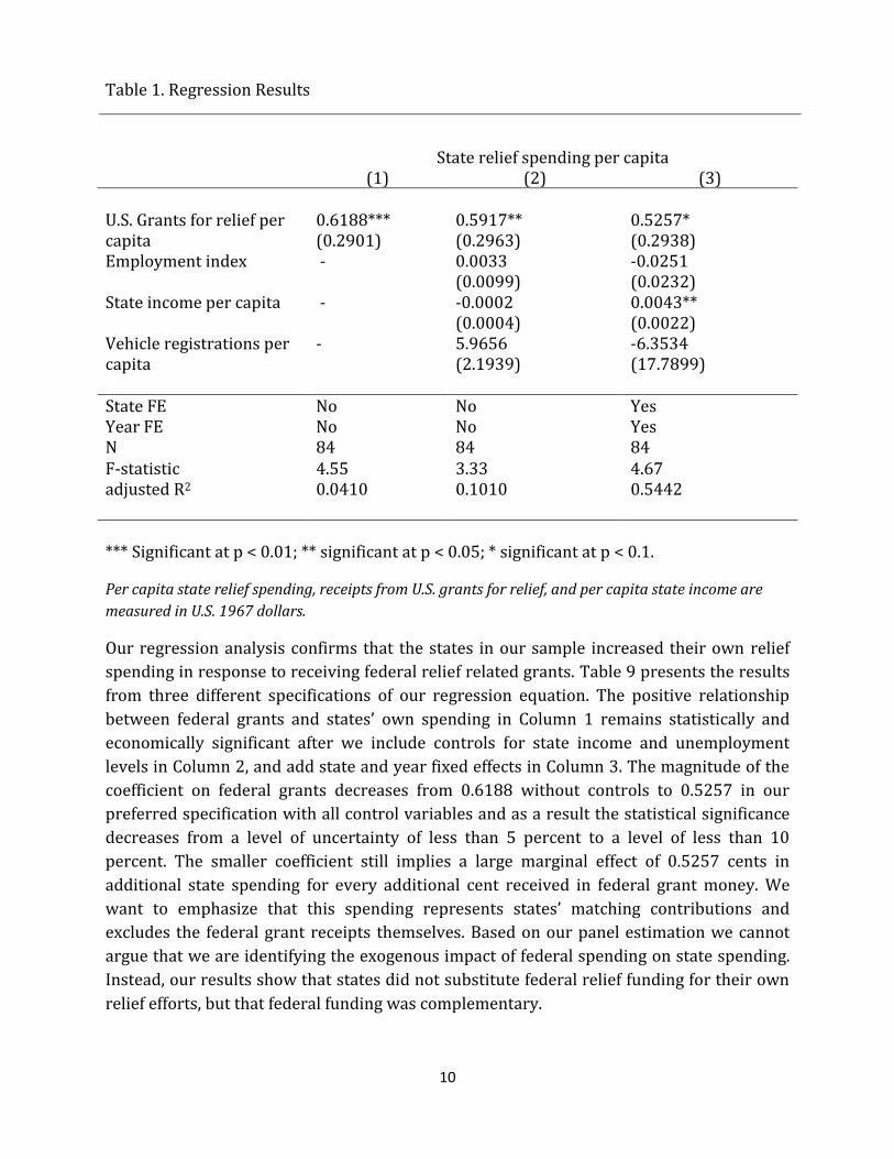
Table 1. Regression Results
State relief spending per capita (1) (2) (3)
U.S. Grants for relief per capita
0.6188*** (0.2901)
0.5917** (0.2963)
0.5257* (0.2938)
Employment index - 0.0033 (0.0099)
-0.0251 (0.0232)
State income per capita - -0.0002 (0.0004)
0.0043** (0.0022)
Vehicle registrations per capita
- 5.9656 (2.1939)
-6.3534 (17.7899)
State FE No No Yes Year FE No No Yes N 84 84 84 F-statistic 4.55 3.33 4.67 adjusted R2 0.0410 0.1010 0.5442
*** Significant at p < 0.01; ** significant at p < 0.05; * significant at p < 0.1.
Per capita state relief spending, receipts from U.S. grants for relief, and per capita state income are
measured in U.S. 1967 dollars.
Our regression analysis confirms that the states in our sample increased their own relief
spending in response to receiving federal relief related grants. Table 9 presents the results
from three different specifications of our regression equation. The positive relationship
between federal grants and states’ own spending in Column 1 remains statistically and
economically significant after we include controls for state income and unemployment
levels in Column 2, and add state and year fixed effects in Column 3. The magnitude of the
coefficient on federal grants decreases from 0.6188 without controls to 0.5257 in our
preferred specification with all control variables and as a result the statistical significance
decreases from a level of uncertainty of less than 5 percent to a level of less than 10
percent. The smaller coefficient still implies a large marginal effect of 0.5257 cents in
additional state spending for every additional cent received in federal grant money. We
want to emphasize that this spending represents states’ matching contributions and
excludes the federal grant receipts themselves. Based on our panel estimation we cannot
argue that we are identifying the exogenous impact of federal spending on state spending.
Instead, our results show that states did not substitute federal relief funding for their own
relief efforts, but that federal funding was complementary.
11
The coefficients on the control variables provide additional support for our interpretation.
In Column 3, per capita income carries a positive and statistically significant coefficient,
indicating that states which experienced higher income recoveries between 1938 and 1939
increased own relief spending by more than states with lower recoveries. Controlling for
employment, per capita income serves as a proxy for the tax base from which the state
raises its revenue. The positive coefficient is therefore consistent with increases in tax
revenue having a positive impact on states own relief spending. The employment index
itself carries a negative although statistically insignificant coefficient, consistent with
decreases in employment causing increases in state relief spending, which includes
unemployment relief and employment services.
6. Conclusion
New Deal programs provided federal funding for public relief, which had been organized
and funded at the local level prior to the Great Depression. These programs included
matching provisions that required states to finance a share of relief expenditures using
their own funds. However, federal reports indicate that these matching provisions were not
fully enforced. Furthermore, states could substitute spending under New Deal programs for
state level relief initiatives that they had started before receiving federal funds. Therefore,
it is unclear whether federal funding was complementary to state spending or acted as a
substitute.
We find that a one cent increase in per capita receipts from federal grants raised states’
own relief spending by $ 0.53 cents. Our result is slightly larger, but similar to Wallis
(1984) estimate of $ 0.34, which is based on data from the “Financial Statistics of States”
from 1937 to 1940. We cannot find out directly how states financed the new relief
expenditures, but we observe the changes in state revenues from different income sources
between 1933 and 1938. Our data show that state tax revenues increased substantially
during this period, which suggests that the states were raising additional revenue to
support new spending programs.
References:
Dorn, R.D. A New Deal for the Glass City: Local Initiatives for Federal Aid during the Great
Depression in Toledo. University of Toledo M.A. Thesis, 1992
Fishback, P.V. and Wallis J.J. What was new about the New Deal? In Crafts, N., and Fearon,
P., (Eds.) The Great Depression of the 1930s: Lessons for today. Oxford University Press,
2013
12
Fishback, P.V. "US Monetary and Fiscal Policy in the 1930s." Oxford Review of Economic
Policy 26.3 (2010): 385-413
Fishback, Price V. The New Deal. In Government and the American economy: A new history.
University of Chicago Press,2008
Fishback, P.V., and Thomasson, M. Social welfare: 1929 to the present. In Historical
Statistics of the United States: Millennial Edition 2, 2006
Margo, Robert A. "The microeconomics of depression unemployment." The Journal of
Economic History 51.02 (1991): 333-341
Maurer, D.J., 1975. Relief Problems and Politics in Ohio. In: Braeman, J., Bremner, R.H.,
Brody, D. (Eds.), The New Deal: The State and Local Levels, volume two. Ohio State
University Press, Columbus OH, pp. 77-102.
Wallis, John Joseph. "The birth of the old federalism: financing the New Deal, 1932–1940."
The Journal of Economic History 44.01 (1984): 139-159.
13
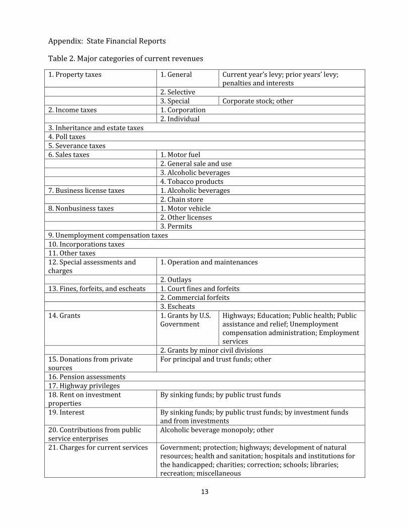
Appendix: State Financial Reports
Table 2. Major categories of current revenues
1. Property taxes 1. General Current year’s levy; prior years’ levy; penalties and interests
2. Selective 3. Special Corporate stock; other
2. Income taxes 1. Corporation 2. Individual 3. Inheritance and estate taxes 4. Poll taxes 5. Severance taxes 6. Sales taxes 1. Motor fuel 2. General sale and use 3. Alcoholic beverages 4. Tobacco products 7. Business license taxes 1. Alcoholic beverages 2. Chain store 8. Nonbusiness taxes 1. Motor vehicle 2. Other licenses 3. Permits 9. Unemployment compensation taxes 10. Incorporations taxes 11. Other taxes 12. Special assessments and charges
1. Operation and maintenances
2. Outlays 13. Fines, forfeits, and escheats 1. Court fines and forfeits 2. Commercial forfeits 3. Escheats 14. Grants 1. Grants by U.S.
Government Highways; Education; Public health; Public assistance and relief; Unemployment compensation administration; Employment services
2. Grants by minor civil divisions 15. Donations from private sources
For principal and trust funds; other
16. Pension assessments 17. Highway privileges 18. Rent on investment properties
By sinking funds; by public trust funds
19. Interest By sinking funds; by public trust funds; by investment funds and from investments
20. Contributions from public service enterprises
Alcoholic beverage monopoly; other
21. Charges for current services Government; protection; highways; development of natural resources; health and sanitation; hospitals and institutions for the handicapped; charities; correction; schools; libraries; recreation; miscellaneous
14
Table 3. Major categories of current cost payments
1. Government 1. Legislative
Legislature; legislative investigation; interstate cooperation
2. Executive Chief executive; auditor or comptroller; board of control; civil service
3. Judicial Supreme court 2. Protection of persons and property
1. Police
2. Fire marshal 5.
Regulation Corporations; occupations; sale of feed, gas, alcoholic beverages; mine and factory inspections; immigration
3. Highways 1. Roadways 2. Waterways 4. Development of natural resources
1. Agriculture
Extension service; experiment stations; livestock; reclamation
2. Forestry 3. Fish and game 4. Geological survey 5. Health and Sanitation 1. Vital statistics 2. Communicable diseases Non-hospital treatment of
tuberculosis 3. Child health service Maternal and child health 4. Regulation Food, occupations 6. Hospitals and inst. for handicapped
1. General hospitals
State, other
2. Special hospitals
1.Insane State, other 2.
Communicable diseases
1. Tuberculosis State, other 2. Other State, other
3. Institutions for the handicapped
Blind; deaf and mute; dumb
7. Charities 1. State institutions 2. Other 1. Public
assistance General relief; old age assistance; dependent children; blind; veterans
2. Grants to min. civ. div.
General relief; old age assistance; dependent children; blind;
3. Grants to private inst.
General relief; old age assistance; dependent children; blind;
4. Welfare services
Child welfare; children in foster and boarding homes
8. Correction Minors; adults; parole boards 9. Schools Grants to minor civil divisions; other 10. Libraries State; other 11. Recreation Cultural; parks and reservations; 12. Miscellaneous Pensions to state employees; unemployment compensation and
employment services; unclassified; undistributed
Source: United States. Bureau of the Census, Financial Statistics of States, Government
Printing Office, Washington D.C., 1937
15
Table 4. Summary of Maryland’s current revenue receipts
Data Year Total Taxes Special Assessments
Federal and minor
civil division
grants
Rental property
Interest payments
Charges for current
services
State Comptroller Reports
1930 31,143,559 22,171,916 568,915 672,733 2,625 448,007 7,279,363 1931 34,731,876 23,909,798 487,776 728,824 2,000 333,628 9,269,851 1932 33,541,535 23,732,783 538,964 777,370 500 190,742 8,301,176 1933 29,397,807 21,471,002 424,704 813,314 1,000 174,662 6,513,123 1934 47,944,400 23,129,613 398,137 2,562,527 1,042 92,152 7,430,806 1935 51,847,908 24,997,017 415,356 3,357,568 1,042 92,314 6,228,085 1936 42,006,789 29,292,744 353,282 4,079,545 1,021 445,183 5,830,463 1937 48,075,425 30,788,972 641,438 5,281,393 1,521 1,795,041 9,457,966 1938 51,370,440 32,124,030 775,929 6,338,309 2,000 1,792,026 10,016,449 1939 52,126,926 32,409,713 616,687 6,989,668 2,000 95,285 11,777,466 1940 55,312,215 39,355,560 737,702 6,054,982 0 92,062 8,631,831
U.S. Financial Statistics of States
1930 30,759,597 20,031,622 343,640 1,123,940 12,742 436,653 4,782,080 1931 33,064,108 24,074,132 1,504,408 2,611,707 11,478 296,789 4,565,592
Interruption 1932 - 1936 1937 48,778,527 37,187,915 329,723 6,426,285 8,361 307,637 4,211,818 1938 57,322,000 44,426,000 382,000 7,572,000 9,000 642,000 3,829,000 1939 61,157,000 47,516,000 32,500 5,855,000 12,000 202,000 2,345,000 1940 76,219,583 58,841,000 43,000 4,614,707 22,000 207,000 2,201,045
All figures are in current U.S. dollars.
Sources: State of Maryland, "Annual report of the Comptroller of the Treasury Department for the Fiscal Year ended June 30 […] to the
General Assembly of Maryland", STATEMENT A : Receipts into the Treasury During the Fiscal Year ended June 30 […]”, 1930 – 1940
(See appendix for the classification of the budget line items); U.S. Bureau of the Census, “Financial Statistics of States […]”,1930 - 1940
16
Table 5. Maryland’s current revenue receipts from taxes
Data Source Year Total Tax Revenue
Property Taxes
Income Tax Death Taxes Sales Taxes Business Licenses
Nonbusiness Licenses
State Comptroller Reports
1930 22,171,916 6,996,573 0 1,508,607 8,748,289 1,756,374 3,153,030 1931 23,909,798 6,843,006 0 2,269,711 9,809,172 1,750,527 3,204,449
1932 23,732,783 6,395,624 0 2,938,303 9,561,050 1,553,530 3,163,771
1933 21,471,002 5,262,736 0 2,875,069 8,407,098 1,618,596 2,976,201
1934 23,129,613 6,143,338 0 1,709,503 10,162,019 1,690,957 3,217,780
1935 24,997,017 5,689,479 0 1,080,979 11,170,132 3,567,510 3,366,028
1936 29,292,744 5,660,986 0 1,419,106 12,520,396 5,900,353 3,693,873
1937 30,788,972 5,928,404 3,377 1,771,377 14,448,451 4,312,809 4,221,504
1938 32,124,030 6,404,899 1,012,242 2,193,392 14,316,720 3,662,007 4,454,837
1939 32,409,713 6,600,017 881,222 2,003,919 14,928,165 3,465,388 4,418,208
1940 39,355,560 5,796,367 7,633,867 1,904,309 17,192,980 2,053,283 4,713,077
U.S. Financial Statistics of States
1930 22,807,838 9,038,173 0 0 0
1,852,975 n.a. 11,335,533 2,434,132 1931 24,074,132 6,526,654 0
0 0
2,161,832 n.a. 12,435,908 2,460,219
Interruption 1932 - 1936
1937 37,187,915 6,111,969 5,577 1,589,330 11,892,012 5,751,671 4,171,868
1938 44,426,000 6,584,000 686,000 1,982,000 13,965,000 5,853,000 4,764,000 1939 47,516,000 6,801,000 875,000 1,824,000 14,661,000 5,956,000 4,775,000
1940 58,841,000 5,986,000 7,637,000 1,723,000 16,795,000 6,453,000 4,927,000 All figures are in current U.S. dollars.
Sources: State of Maryland, "Annual report of the Comptroller of the Treasury Department for the Fiscal Year ended June 30 […] to the
General Assembly of Maryland", STATEMENT A : Receipts into the Treasury During the Fiscal Year ended June 30 […]”, 1930 – 1940
(See appendix for the classification of the budget line items); U.S. Bureau of the Census, “Financial Statistics of States […]”,1930 - 1940
17
Table 6. Maryland’s current revenue receipts from income taxation
Data Year
Income Tax (1937 Law) Income Tax 1939 Law Other
Corporations Individual Non-resident Fiduciary Other
State Comptroller Reports
1930 0 0 0 0 0 0 0 1931 0 0 0 0 0 0 0 1932 0 0 0 0 0 0 0 1933 0 0 0 0 0 0 0 1934 0 0 0 0 0 0 0 1935 0 0 0 0 0 0 0 1936 0 0 0 0 0 0 0 1937 0 0 0 0 0 0 3,377 1938 0 0 0 0 0 0 1,012,242 1939 0 0 0 0 874,447 4,656 119 1940 1,304,569 6,197,611 39,184 84,024 8,479 0 0
U.S. Financial Statistics of States
1930 0 0 0 0 0 0 0 1931 0 0 0 0 0 0 0
Interruption 1932 – 1936 1937 5,577 0 0 0 0 0 0 1938 36,000 650,000 0 0 0 0 0 1939 305,000 570,000 0 0 0 0 0 1940 1,392,000 6,245,000 0 0 0 0 0
All figures are in current U.S. dollars. Sources: State of Maryland, "Annual report of the Comptroller of the Treasury Department for the Fiscal Year ended June 30 […] to the General Assembly of Maryland", STATEMENT A : Receipts into the Treasury During the Fiscal Year ended June 30 […]”, 1930 – 1940 (See appendix for the classification of the budget line items); U.S. Bureau of the Census, “Financial Statistics of States […]”,1930 - 1940
18
Table 7. Maryland’s current revenue receipts from sales taxes
Data Year
Gasoline Tax Titling Alcoholic Beverages Gross
Receipts Maintenance,
Reconstruction (2c Tax)
Lateral Roads (1.5c Tax)
Grade Crossing (.5c
Tax)
Motor Vehicle
Other Distilled Spirits
Wine Beer
State Comptroller Report
1930 3,356,231 2,510,792 839,058 169,157 0 0 0 0 1,873,050 1931 3,694,308 2,790,208 933,577 153,732 0 0 0 0 2,237,347 1932 4,028,716 2,979,618 997,179 125,805 0 0 0 0 1,429,732 1933 3,556,281 2,653,291 889,070 124,289 0 0 0 0 1,184,166 1934 4,032,964 3,008,097 1,008,204 141,973 0 912,832 0 0 1,199,922 1935 4,180,630 3,117,736 1,045,158 161,942 0 1,426,419 16,991 0 1,383,199 1936 4,369,618 3,255,449 1,092,275 702,330 0 1,910,434 53,944 0 1,332,620 1937 4,870,318 3,631,764 1,217,580 593,987 216,656 2,522,104 69,882 0 1,542,817 1938 4,972,520 3,707,783 1,243,130 571,955 0 2,367,900 71,609 0 1,556,133 1939 5,198,459 3,874,495 1,299,615 511,860 195,512 2,457,484 100,205 0 1,486,047 1940 5,629,477 4,194,925 1,407,369 1,198,593 227,829 3,137,898 185,873 1,047,043 1,590,394
U.S. Financial Statistics of States
1930 5,866,621 2,285,133 0 0 n.a. 1931 6,514,516 2,383,049 0 0 n.a.
Interruption 1932 – 1936 1937 7,539,492 4,081,461 0 4,097,016 n.a. 1938 9,923,000 4,599,000 0 3,514,000 n.a. 1939 10,373,000 4,585,000 0 3,625,000 n.a. 1940 11,232,000 4,736,000 0 4,362,000 n.a.
All figures are in current U.S. dollars.
Sources: State of Maryland, "Annual report of the Comptroller of the Treasury Department for the Fiscal Year ended June 30 […] to the General Assembly
of Maryland", STATEMENT A : Receipts into the Treasury During the Fiscal Year ended June 30 […]”, 1930 – 1940 (See appendix for the classification of
the budget line items); U.S. Bureau of the Census, “Financial Statistics of States […]”,1930 - 1940
19
Table 8. Summary of Maryland’s current cost payments
Data Year Total Government Police Highways Agriculture and Natural Resources
Health Hospitals1 Charities Prison Schools Employm. services
State Comptroller Report
1930 27,398,468 1,497,493 1,591,177 15,156,956 622,993 484,301 2,556,588 358,462 1,053,123 4,080,360 0
1931 27,015,547 1,579,504 1,745,281 14,189,888 650,362 522,156 2,675,723 385,497 1,068,820 4,278,553 0
1932 34,998,465 1,716,864 1,620,263 14,292,443 777,659 578,694 2,801,898 424,296 1,324,918 11,460,684 0
1933 27,956,775 1,887,386 1,583,691 12,147,194 1,073,429 421,343 2,769,777 413,459 1,143,585 5,172,208 1,231,350
1934 41,075,448 1,935,913 1,427,462 13,121,243 854,880 464,721 2,349,985 403,743 1,088,072 4,395,245 15,137,097
1935 55,276,049 2,095,491 642,166 24,388,490 602,013 476,528 2,119,882 540,373 962,202 6,296,384 17,032,056
1936 50,886,394 1,688,158 1,987,163 9,331,101 568,265 545,315 1,866,020 4,652,275 1,042,305 6,676,006 21,709,887
1937 36,324,240 1,703,487 1,222,109 12,376,940 564,355 1,674,512 2,056,699 8,180,996 1,205,759 6,371,780 209,832
1938 41,910,776 1,472,926 1,362,978 13,063,668 851,873 745,772 2,411,640 9,268,682 1,819,230 8,941,397 1,120,603
1939 46,469,868 1,991,118 1,327,056 12,434,256 825,217 785,710 2,870,869 13,050,929 1,928,562 9,297,798 1,051,383
1940 n.a. n.a. n.a. n.a. n.a. n.a. n.a. n.a. n.a. n.a. n.a.
U.S. Financial Statistics o f States
1930 21,579,370 2,284,966 1,215,570 6,297,012 1,157,540 1,139,335 2,128,385 243,662 852,265 5,543,483 0
1931 21,651,132 2,567,286 1,417,278 5,033,402 1,236,774 1,211,931 2,241,023 417,181 1,019,810 6,079,365 261,965
Interruption 1932 – 1936
1937 28,426,967 1,545,809 1,479,459 4,248,074 1,077,014 784,977 3,325,555 6,376,893 1,169,145 7,194,532 193,475
1938 44,108,000 1,273,000 1,833,000 7,305,000 1,191,000 871,000 3,561,000 7,267,000 1,614,000 8,376,000 9,572,000
1939 42,573,000 2,719,000 1,700,000 4,973,000 1,092,000 914,000 3,525,000 7,996,000 1,700,000 8,614,000 7,444,000
1940 45,242,000 1,734,000 1,685,000 9,152,000 1,373,000 998,000 3,615,000 8,421,000 1,731,000 8,701,000 7,456,000
1 Hospitals include institutions for handicapped.
All figures are in current U.S. dollars.
Sources: State of Maryland, "Annual report of the Comptroller of the Treasury Department for the Fiscal Year ended June 30 […] to the General Assembly
of Maryland", STATEMENT A : Receipts into the Treasury During the Fiscal Year ended June 30 […]”, 1930 – 1940 (See appendix for the classification of
the budget line items); U.S. Bureau of the Census, “Financial Statistics of States […]”,1930 - 1940
20
Table 9. Maryland's current cost payments for relief
Data Year Total Public Assistance Grants1 Child welfare Other
Admin. Old age Child Blind Veteran Other Old Age Child Blind Other General Homes
State Comptroller Report
1930 358,462 0 0 0 0 0 0 28,500 327,162 0 2,800 0 0 0
1931 385,497 0 0 0 0 0 0 27,563 355,134 0 2,800 0 0 0
1932 424,296 0 0 0 0 0 0 30,250 391,246 0 2,800 0 0 0
1933 413,459 0 0 0 0 0 0 23,866 386,793 0 2,800 0 0 0
1934 403,743 0 0 0 0 0 0 22,530 379,325 0 1,888 0 0 0
1935 540,373 0 0 0 0 0 0 20,095 510,472 0 9,806 0 0 0
1936 4,652,275 0 446,762 395,958 24,327 0 1,752,410 0 0 1,194,215 15,658 0 822,943
1937 8,180,996 0 1,471,289 909,188 81,405 0 4,392,474 0 0 0 1,202,687 123,208 0 74,547
1938 9,268,682 0 61,252 1,023,294 76,709 0 6,720,432 0 0 0 1,312,625 74,182 0 1,872
1939 13,050,929 0 1,946,677 1,179,278 85,034 0 7,636,821 0 0 0 1,307,600 130,744 0 764,774
1940 n.a. n.a. n.a. n.a. n.a. n.a. n.a. n.a. n.a. n.a. n.a. n.a. n.a. n.a.
U.S. Financial Statistics Of States
1930 243,662 0 0 0 121,162 0 0 122,500 3,500 106,556 0 0 0
1931 417,181 0 0 0 149,384 0 0 122,250 94,797 3,500 47,250 0 0 0
Interruption 1932 - 1936
1937 6,376,893 563,459 0 0 0 101,702 931,020 2,521,683 2,136,451 79,795 0 18,268 0 3,500
1938 7,267,000 0 0 18,000 80,000 0 34,000 2,934,000 2,535,000 84,000 1,110,000 22,000 0 4,000
1939 7,996,000 287,000 34,000 146,000 78,000 96,000 0 3,058,000 2,567,000 105,000 1,243,000 24,000 0 4,000
1940 8,421,000 13,000 28,000 142,000 78,000 96,000 0 3,381,000 2,781,000 0 1,258,000 126,000 54,000 3,000
1 The appropriation acts in Maryland’s session laws of the regular session 1929 (chapter 134, p.275) and 1935 (chapter 92, p.172) indicate that the
grants identified from the comptroller reports are made to private, charitable organization (state-aided institutions). In the U.S. Financial Statistics of
States, the category refers to grants to minor civil divisions.
All figures are in current U.S. dollars.
Sources: State of Maryland, "Annual report of the Comptroller of the Treasury Department for the Fiscal Year ended June 30 […] to the General Assembly
of Maryland", STATEMENT A : Receipts into the Treasury During the Fiscal Year ended June 30 […]”, 1930 – 1940 (See appendix for the classification of
the budget line items); U.S. Bureau of the Census, “Financial Statistics of States […]”,1930 - 1940