Figure 1: Astronaut Bean examiningSurveyor III. Note that the Apollo 12 LM

is in the background.

Further Analysis on the Mystery of the Surveyor III Dust Deposits

Philip Metzgerl, Paul Hintze l

, Steven Trigwele, John Lane3

1Granular Mechanic and Regolith Operations Lab, NASA, Kennedy Space Center, FL 328992 Applied Technology, Siera Lobo-ESC, Kennedy Space Center, FL 328993 Granular Mechanics and Regolith Operations, Easi-ESC, Kennedy Space Center, FL 32899

ABSTRACT

The Apollo 12 lunar module (LM) landing near the Surveyor 1lI spacecraft at the end of 1969 has remained theprimary experimental verification of the predicted physics of plume ejecta effects from a rocket engine interactingwith the surface of the moon. This was made possible by the return of the Surveyor 1lI camera housing by theApollo 12 astronauts, allowing detailed analysis of the composition of dust deposited by the Apollo 12 LM plume.It was soon realized after the initial analysis of the camera housing that the LM plume tended to remove more dustthan it had deposited. In the present study, coupons from the camera housing were reexamined by a KSC researchteam using SEMIEDS and XPS analysis. In addition, plume effects recorded in landing videos from each Apollomission have been studied for possible clues. Several likely scenarios are proposed to explain the Surveyor III dustobservations. These include electrostatic attraction of the dust to the surface of the Surveyor as a result ofelectrostatic charging of the jet gas exiting the engine nozzle during descent; dust blown by the Apollo 12 LM fly-bywhile on its descent trajectory; dust ejected from the lunar surface due to gas forced into the soil by the Surveyor 1lIrocket nozzle, based on Darcy's law; and mechanical movement of dust during the Surveyor landing. Even thoughan absolute answer is not possible based on available data and theory, various computational models are employedto estimate the feasibility of each of these proposed mechanisms. Scenarios are then discussed which combinemultiple mechanisms to produce results consistent with observations.

BACKGROUND

In 1967, an unmanned robotic landing device known as Surveyor III, lifted off from thefor Earthon April 17 and landed on the moon on April 20. The location of the Surveyor III landing was atthe Mare Cognitum portion of the Oceanus Procellarum (30 01' 41.43S" 23° 27' 29.55"W).Surveyor III transmitted 6,315 photographic imagesback to the Earth.

The landing of the Surveyor III was far from smooth.According to Wikipedia:

As Surveyor III was landing (in a crater, as it turnedout), highly reflective rocks confused the spacecraft'slunar descent radar. The engines failed to cut off at 14feet (4.3 meters) in altitude as called for in the missionplans, and this delay caused the lander to bounce on thelunar surface twice. Its first bounce reached the altitudeof about 35 feet (10 meters). The second bouncereached a height ofabout 11 feet (three meters). On thethird impact with the surface - from the initial altitudeof three meters, and velocity of zero, which was be/owthe planned altitude of 14 feet (4.3 meters), and veryslowly descending -Surveyor III settled down to a softlanding as intended.

1

https://ntrs.nasa.gov/search.jsp?R=20120000029 2018-06-23T15:59:36+00:00Z

For over 2 years, Surveyor III simply resided on the surface being exposed to the ravages ofspace. However, on November 14, 1969, Apollo 12 launched from the Earth (despite beingstruck twice by lightning during take-off) and landed on the moon on November 19, 1969 atOceanus ProcellarumlMare Cognitium (Ocean of StormslKnown Sea) at coordinates 3°00'45"S23°25'18"W or 3.012389°S 23.421569°W. The Lunar Module (LM) of the Apollo 12 namedIntrepid purposely landed 155 m to the west from Surveyor III. Apollo 12 astronauts Charles"Pete" Conrad (Commander) and Alan L. Bean (LM Pilot) were able to examine Surveyor III (asshown in Figure 2) and bring parts back to the Earth. It is interesting to note that theseismometers the astronauts had left on the lunar surface registered the vibrations from the LMlift-off for more than an hour.

The relative landing sites of theApollo 12 LM and Surveyor III areshown in Figure 2. The astronautsvisited the Surveyor IlIon theirsecond excursion. Lunar sampleswere taken throughout theexcursions totaling a combinedweight of 34 kg of rocks, soil, andcore samples (taken down to 40 embelow the surface regolith). Achemical analysis of most of thesamples can be found on the Lunarand Planetary Institute website(http://www.lpi.usra.edu/lunar/missi

ons/apollo/apollo_12/samples).Figure 2: Landing sites of Intrepid and Surveyor III. Samples taken near the LM and

others taken near to Surveyor IIIhave been tabulated in Appendix A. The goal is to observe if the elemental analysis from XPSand SEMlEDX done in the present study correlates with soil/rocks either near the LM site ornear the Surveyor III site.

LU AR SURVEYOR III SAMPLES

The Surveyor III parts brought back to Earth by Apollo 12 are currently stored at the JohnsonSpace Center (JSC) Lunar Sample Curation (http://www-curator.jsc.nasa.gov/lunar /index.cfrn),and information on the chemical analyses is found at the Lunar and Planetary Institute(http://www.lpi.usra.edu). Several of the parts were requested and sent to KSC for analysis inthe present study (see and Figures 3 and 4). Those parts are summarized in Table 1.

2

I~11

Figure 3: The camera module showing the bottom cutout.

I Figure 4: Surveyor III camera on the mOOD.

Table 1. Surveyor III Parts Under Investigation.

Type of Sample Part Designation Comments

JPL#1037Sample from the camera

bottom.

JPL #2048 Flat side of camera.

JPL #2049Sample from camera pointing

Cutouts from the Surveyor away from the Apollo 12 LM.

III Camera JPL #2050 (JSC #3160026)Sample from camera pointing

towards the Apollo 12 LM.

JPL #2051 (JSC #3160027)Sample from camera pointing

towards the Apollo 12 LM.

JPL #2052Sample from camera pointingaway from the Apollo 12 LM.

Acetate Tape Samples of 327082 052the Regolith Material

(collected from underneath327 083 053

the camera clamp)

Section of Cylindrical RodSample from each end

(strut for the radar)

PARTICLE MODELING AND SIMULATION

Shear Stress Simulations of LM Engine Plume Flyby

Starting with a Fluent CFD simulation of the Apollo LM engine in a lunar-like environment(background pressure is artificially set to a small non-zero value in order to achieve

3

convergence), three gas parameters are computed for every point in a 2D non-uniform spatialgrid: gas density fi...k), gas temperature T(k), and gas velocity v(k). Each CFD simulation andcomputed gas parameter output set corresponds to a specific engine height h above the lunarsurface. The CFD simulation generates gas parameter data at specific spatial pointscorresponding to the x-y coordinates contained in the grid point array, r(k). Note that for theFluent CFD cases considered in this report, vertical positions are described by the coordinate xand horizontal positions are described by the coordinate y. Since the CFD generation of spatialpoints is based on algorithms which are used to minimize error in partial differential equationsdescribing the laws of fluid mechanics, the grid points for all practical purposes are randomlydistributed. Therefore, finding a specific point nearest a field point x-y and its nearest neighbors,involves searching'the entire r(k) array for k = 1... N.

To compute the shear stress from the CFD output, the grid data is resampled along the lunarsurface boundary at rmn = (mtu, n~y) for m = 0, 1, 2 and n = 0... Nx . The shear stress isdefined by:

avT == /l ---.1::. (1)ax

where fl is the dynamic viscosity of the gas, vy is the horizontal component of the gas velocityalong the horizontal surface boundary, and x is the distance above the surface. The gasdynamic viscosity is a function of temperature and can be computed by Sutherland's formulaapproximation:

~ + C (T)3/2/l(T) == /lo ; + C To

where the parameters flo, C, and To are dependent on the gas composition.

A discrete approximation to the shear stress of Equation (1) can beresampled CFD output:

v -vY2n YOnT ==Iln' ,

n 2L1x

where

(2)

computed usmg the

(3)

_ To + C (T1,n)3/2 (4)/In = /lo T + C ~

1,n 0

An equivalent shear velocity (sometimes referred to as saltation velocity) can be computed fromEquation (3) and the resampled gas density:

SIMULATION RESULTS

( )

1/2Tn

Un= ­P1,n

(5)

Shear stress along the surface has been computed for the five cases generated by Fluent CFD: h= 5, 10, and 20 [ft] and h = 25 and 45[m). The shear stress is computed and plotted for these

4

.-------------------~-----------------------------------

five cases in Figure 16. The shear stress in this figure was generated with & = 0.001 [m] inEquation (3).

Shear Stress Using Sutherland's Formula for Dynamic Viscosity100

1412

<-- CFD Domian End --->

10

- Cl (h =20ft)- C7(h= 10ft)- C2(h =5ft)- LM Fly-by (h = 25 m)- LM Fly-by (h = 45 m)

8

10

co!hIf)If)

~:;;Q>

0.1-'=(f)

0.01

0.001

0 2 4 6

Distance from Nozzle [m)

Figure 5: Shear stress along the x = Ax surface for five cases generated by FluentCFD: h = 5, 10, 20, 25, and 451ft).

Threshold Shear Stress Velocity

Starting with the approach of Sagan (1990), the threshold shear stress velocity is:

(5)

where,

(6)

and,

A. - 3'Pi = az rJ (7)

The gas kinematic viscosity is the gas dynamic viscosity divided by its density: rJ = 11/p. WithEquation (5) and its variables expressed in SI units, the constant coefficients are given in Table2.

5

Table 2. Coefficients in Equations (5) and (7).

ao 2/15

al 8.3995

az 250000

a3 843750

a4 0.0021165

The result in Sagan (1990) was greatly simplified with the assumption that the Reynolds numberis much less than 1: , or . Equations (5) through (7) do not makethat assumption. The threshold shear stress velocity of Equation (5) can be converted into athreshold shear stress, similar to that of Equation (5):

(8)

The cohesion force (interparticle force) in Sagan (1990) is approximated as:

(9)

where again, Equation (9) and its variables are all expressed in SI units. Sagan (1990) used avalue of fJ = 6x 10-7 to represent the cohesive force of particles on the surface of Triton. Tosimulate a zero cohesion force, fJ is set equal to zero.

SIMULATION RESULTS

Figure 17 shows the trajectory simulation results: the radial distance traveled by particle fromground track position as a function of particle diameter. Circles represent different startingpoints, both x and y, while the solid line is the average maximum value of the individualtrajectories. Note that there is a notable cut-off as the particle size approaches 100 /lm.

I."..1i>

~.. ,gBe5 01

!

) .. ) .,..1

) .. ) , 1 It10

1 J .. •• '"100

o [um)

Figure 6: Radial distance traveled by particle from ground track position as a function of particlediameter for h = 45 m. Circles represent different starting points, both x and y. Solid line is the

average maximum value of the individual trajectories.

6

Figure 18 shows post-processed results of a Fluent CFD simulation corresponding to the Apollo12 LM flyby at h = 45 [m]. Note that the actual height of the closest approach distance from theLM ground track to the Surveyor III site is approximately h = 65 [m]. (h = 65 [m] Fluent CFDresults were not available during the project period). Referring to Figure 18, the left axis andblue line represents the radial distance traveled by a particle from the ground track position. Theshaded portion represents all particles whose horizontal trajectory distance is equal to or greaterthan the distance to the Surveyor spacecraft (R = 109 [mD.

The right axis corresponds to the difference in shear stress, Equation (3) and threshold shearstress, Equation (8), indicating the region where lift may occur without the need of particlecollisions to initiate a lift process. The zero cohesion force case is shown by the green line andgreen shading. Sagan's cohesion force, using fJ = 6x10-7

, is shown by the brown line andshading.

h=45m- Average Max Horlzonlal Distance Traveled

Average Max Threshold Lin Shear Stress- Average Max Threshold un Shear Stress (Cohesion Force =0)

1

•,•s

C\I

':;j"0.1

•,

I_ ~=.102 ITI. _

1

•,:l ~~---"Cohe~~sIon~For~c:!!..o~' o~.....::::::::::- Sagan Cohesion

10' 10'Dblln)

10' 10'

Figure 7: LM Flyby simulation at h = 4S [mI. Left axis: (blue line) radial distance traveled by particlefrom ground track position. Right axis: (green and brown lines) region where shear stress is greater than

threshold shear stress, resulting in particle lift for zero cohesion force (green line) and for Sagan'scohesion force (brown line).

Discussion

Based on particle trajectory simulations for the h = 45 m case (the h = 65 m case was notcompleted, possibly due to numerical convergence problems), dust reaches the Surveyor III sitefrom the LM flyby closest approach (R = 109 m). Particle sizes up to D = 13 urn reach theSurveyor III with velocities up to 130 mls. Particles sizes D > 13 urn, are also ejected, but fallback to the surface before traversing the complete 109 m distance to the Surveyor. Particles inthe size range of 17 < D < 2600 /lm can be lifted by the gas shear stress, bas~d on the h = 45 mFluent CFD case. According to the plots in Figure 18, there is no particle size range that showsan overlap between the trajectory distance and threshold shear stress for R = 109 m. Inspectingthe plot in more detail, particles of D = 20 /lm would reach a distance ofR = 80 m.

7

,----------------------------------------------------

Sagan's cohesion force (Iversen,1982) predicts interparticle cohesion forces on the order of nNfor particles in the range of 10 - 100 J..lm. Sagan's cohesion force is about a 1000 times smallerthan the cohesion force predicted by Walton (2008), which predicts J..lN particle pull-off forces(see Figure 19). Even for the small Sagan cohesion force (~ nN for 10-100 J..lm particles),particles do not make it to the Surveyor III site, unless the cohesion force is much smaller(maybe a factor of 10 smaller would do it). But a factor of 1000 larger would certainly decreasethe chance of particle spray from the LM flyby.

K = 6xl(t7 [NlmlnjIt =SI2mnm. J.D, B.ll.~ "SIlIIdaa.DIaboId OIl F.IIlb.M...... Vcna'".,y ·,q,.19. 1912,,,. 111·119.

F. =21f'JlJ

r = 0.075 [JIm"]w....Olt. -lniawofAdlaiuDf\w..." ."'11 IbrMboa-Sealohrticb-,Powlcb-lIIIIIl'Irtide JourmI,. Z6"20C*,pp.I29-J41.

I =K D)-",

D[m]5x 10-4 Ix 10-5 )x 10-5

II I I I I III I -f--r 1111111

II ......+-rllllli I I I I I III11

II I I I I III I I I I I II III

II I I I I I III I I I I I III1I

I I I-- I I I

10-5

Figure 8: Comparison between Iverse (1982) interparticle cohesion forces and cohesion pull-off forcepredicted by Walton (2008).

DARCY'S LAW

Darcy's Law describes the volume flow rate Qof a gas or liquid of viscosity JL through a solidporous medium of permeability K, due to a pressure gradient over a length tiL:

(D1)

where A is the cross-sectional area of the flow volume and M/tiL is the pressure gradient.Darcy's Law can be used to describe the portion of gas that is injected into the soil immediatelybeneath the rocket nozzle. Since Q in Equation (D 1) can be replaced by the gas velocity vet)scaled by A, the initial velocity at t = 0 is:

(D2)

Immediately before engine cutoff, the pressure on the surface due to the lander's rocket gasimpingement at t = 0 can be approximated as:

(D3)

8

(D4)

.-------------------------------------------------

where M is the mass of the lander, g is acceleration due to lunar gravity, and A is the area on thesurface over which the pressure is acting. Combining Equations (D2) and (D3):

KMgVo = - /lI1LA

The trajectory of regolith particles lifted upwards from the surface after engine cutoff due to therelease of plume gas trapped in the soil can be computed by considering Newton's second law ofmotion, F = rna. F for can be expressed as the gas pressure at the surface due to the trapped gasbelow as, pv2(t)/2, where p is the gas density. The term rna can be expressed as (pA L) dv(t)/dt,which then leads to:

dv(t)

dt

V(t)2---

2L(D5)

(D?)

where the minus sign is needed because of velocity decreasing. The solution to Equation (D5)1S:

Vovet) - (D6)

v ot/2L + 1

Equation (D5) is an approximation the velocity of a particle lifted from the surface due to theDarcy effect, immediately following engine cutoff.

A single particle trajectory can be obtained by computing the position as a function of time byevaluating the integral of velocity from 0 to t:

y(D, t) = l\V(t') - vr(D))dt'

where y(D, t) is the vertical position of the particle and vy{D) is its terminal velocity in the gasflow. Note the particle diameter dependence of the terminal velocity term. The above integralcan be evaluated as:

y(D, t) = 2L In(vot/2L + 1) - vr(D)t (D8)

The terminal velocity term is due to the drag on the particle by the gas and the pull of lunargravity. Since the gas density is very small as compared to the particle density PP' the terminalvelocity vy{D) depends only on gas viscosity j.1,(T), as given by Equation (2), as well as gravity gand particle diameter D:

(D9)

To demonstrate the ideas described above, Apollo landing videos can be used. Figure DI showsa view captured by the Apollo 14 cockpit camera immediately after engine cutoff. Theluminosity value L(t) is found in two regions of the image at t = 0 and again at t = 34 s. The righthistograms corresponds to a region imaged inside of the LM, part of the window frame. Thehistograms on the left correspond to a shadowed region on the lunar surface partly obscured bydust. Figure D2 plots the normalized relative luminosity, Lt/..t) = (L(t) - Loo)/Lo , over severalframes. In this case, Lo= L(O) and Loo = L(34). For comparison, a dust particle falling freelyunder lunar gravity from a height Yo = 10m is shown, where yet) = Yo - g P/2. Also plotted in

9

Figure D2 is Equation (D8) for several values of particle diameter with a temperature T = 250 K,A = 1 m2

, M = 0.2 m, K= 10 /1JJi, fJp = 3100 kg/m3, and M= 14 metric tons.

Mun: 8•.25 ltv": Ltv":std C.VI 2-'4 C.,....: C.,....:

Mt<bnl 8. PfrCnNl Pt<etnlilt,

1'.,,'" 50' C.c:ht ltvtt: 1 C_to•." I

Histoorwn H1tOO'aM

o..nn.I, l.-...ty V ...

[ ]Mt,anl ...... L...II lenl:

Stdo.VI 157 C.,...., C.,....,

Mldi.anl oW Pwcotdo, Pwcotdo,1',..1" 351 C_L..." I CdMLnth 1

Figure 9: Luminosity measurements of Apollo 14 landing videos following engine cutoff.

10

, ,.•

t-t... -""" --...~F-!: --i'...n", ~ tim

~;...-- - =.----- I \ '\

I

1\ 1\ 1-...,

, ,~ lo,'./1 Ullf,

-ll to·/( ,}id~Q,

1.0

0.1

0.01

1 10Elap:ed Time ti-om Engine Shutoft: f [s]

100

Figure 10: Freefall and Darcy law particle trajectories compared to luminosity.

10

Discussion

The first conclusion that can immediately be reached by inspection of Figure D2 is that the timerequired for dust clearing to occur is longer by an order of magnitude then would be explainedby freely falling dust under lunar gravity. The same is true for dust under the influence of astatic electric field since the electric field term would more likely decrease the clearing time asopposed to an unlikely balance of electric and gravity forces leading to a longer clearing time.

Dust propelled vertically by the Darcy effect could circumstantially explain the dust clearingsince there are a range of conditions where Equation (D8) matches the clearing timecorresponding to the luminosity values measured in the Apollo 14 video. Ignoring the grossassumptions that led to Equation (D8), the Darcy Law simulations do not show the dusttravelling high from the surface, which for Figure D2 is only in the 10 - 20 cm range. This mayhowever be consistent with the Apollo videos since the main landing dust plume (before enginecutoff) is believed to be contained within a three degree sheath radially centered about thenozzle, which for a distance of 5 m form the nozzle corresponds to dust only up to 25 cm abovethe surface. The dust viewed by the videos before and after engine cutoff, is primarily seen as ahaze over the surface. Another interesting feature in Figure D2 is the dip in the luminosity.Since it is only a single point, it is unwise to declare this an important feature without additionalimage analysis.

SEMSTUDIES

Samples were analyzed via scanning electron microscopy (SEM) and Electron DispersiveX-Rays (EDX) to visually and chemically study several of the Surveyor III samples.

XPS ANALYSIS

X-ray photoelectron spectroscopy (XPS) analysis was performed on areas from 3 cut-outsfrom the Surveyor III camera, namely; parts #2048, #2050, and #2051. Visual observation on theparts showed areas of differing discoloration. As XPS is a very surface sensitive technique,analysis was performed to determine any chemical differences between the areas to explain theapparent discoloration. The areas of analysis are shown in the figures for each part respectively.

The XPS analysis was performed on a Thermo Scientific K-Alpha spectrometer. Thesamples were mounted with care so as to not introduce any surface contamination by handling.The samples were pumped down to a background pressure of 3 x 10-9 torr. The x-rays used werefrom an Al Ka source with an energy of 1486.6 eV. A low energy electron flood gun wasutilized to prevent charging of the surface. A spot size of 400 I!m was used for each analysispoint and wide survey scans were taken to detect all elements of interest. The mean escape depthof the emitted photoelctrons is approximately 50 - 100 A, depending upon the element, and soXPS is a very surface sensntive technique. The areas under the peaks of the detected elementswere measured and the relative atomic concentrations were calulated using sensitivity factorsprovided by the instrument manufacturer. The accuracy of quantification is approximately +/­5% of the determined values. In the approximate areas illustrated in the Figures 21 and 25,thirteen (13) random analysis points were taken and the mean value calculated with the standard

11

•

deviation. For sample #2050 (Figs. 22 and 23), a series of overlapping analysis points were takenin a linescan across the dark shadow region outside the bolt hole.

Sample #2048

The sample is ahown in Fig. 21, and the results of the analysis are shown in Table 3.

Figure 21: Sample # 2048 showing areas of analysis in the light (Area 1) and dark (Area 2) areas.

Table 3: Relative atomic % of elements in Areas 1 and 2 of sample #2048.

01s K2p Si2p AI2p Na1s Mg1s Cls S2s Fe2p CI2p F1s

Area 1 58.42 9.08 16.30 3.19 0.57 0.33 11.51 0.42 0.05 0.07 0.08 Mean

(lighter) 0.12 0.08 0.52 0.21 0.11 0.14 0.68 0.05 0.06 0.10 0.11 SO

Area 2 54.52 9.70 14.29 2.25 0.67 0.69 16.24 0.88 0.21 0.43 0.40 Mean

(darker) 1.85 0.19 0.42 0.04 0.10 0.57 2.55 0.21 0.08 0.01 0.40 SO

The main difference between the lighter and darker areas is a notable increase in the Mg,Fe, Fe, C, S, CI, and F concentrations. The white paint originally applied to the Surveyor III craftwas reported to be composed of aluminum silicate pigment with a potassium silicate binder(Immer, 2010). The AI, Si, 0, and K concentrations can therfore be attributed to the paintcoating. Analysis of Apollo 12 regolith collected during the mission, showed after Al and Sioxides, the next predominant compounds were Fe, Mg, and Ca oxides (Heiken, 1991).Unfortunately, in the above analysis, Ca was not detected due to the signal-to-noise of the

12

spectra had not been optimised, however, the significant increase in the Fe and Mgconcentrations strongly indicate the presence of lunar regolith in the darker area. The two mostabundant minerals in the Apollo 12 regolith after agglutinates, were pyroxene and olivine(Heiken, 1991) that have the chemical formulas, XY(Si,AI)206 (where XY = Ca, Na, Fe, Mg),and (Mg, Fe)2Si04, respectively. The data above also correlates with the presence of these twominerals.

The presence of C, F, S, and CI indicate contamination of the sample, as had beenpreviously reported reflecting the extensive use of fluorocarbons during the Apollo missions andpost-mission sample handling (Goldberg, 1976).

Sample #2050

For this sample, a shadowed region to one side of a bolt hole was observed, as shown inFig. 22. The white region is unexposed paint that was under a washer. In order to determine thenature of this darkened area, survey scans were performed in an overlapping series (linescan)from the white area out through the shadowed darker area to the lighter area. The red line in Fig.22 shows the approximate path of the linescan. The actual analysis points are shown in thehigher magnification photograph in Fig.23.

For these analyses, the acquisition time was increased to improve the signal-to-noise ratioin the spectra so that the Ca peaks were detected and could be quantified. The data was plotted asatomic concentration as a function of the linescan across the region, and is shown in Fig. 24. InFig 24a, the entire data set is included, and in Fig. 24b, the Y-axis was expanded to better showthe variation of the minor elements.

13

Figure 22: Sample # 2050 showing area of linescan across the dark shadow near hole.

Figure 23: Sample # 2050. The linescan analysis started at bottom right. Each analysis point was a 400urn spot size and each point overlapped.

14

70

60

*' 50I:0

',tj

~ 40...QII:uI: 300u,~

E 200:i

10

0

1 2 3 4 5 678Analysis point from hole

9 10 11

-k-Fe2p-k-Ca2p~Nals

___ 015

-,-K2p

--*-Si2p

.....-A12p

....._Mgls

-f-Cls

Figure 24a: Relative atomic concentrations across shadowed section in Fig. 23.

0.7

0.6

*' 0.5I:0~

~ 0.4...QII:uI: 0.30u,~

E 0.20

:i0.1

0

1 2 3 4 5 678Analysis point from hole

9 10

-k-Fe2p

-k-Ca2p

11

Figure 24b: Relative atomic concentrations of Fe and Ca across shadowed section in Fig. 23.

15

In Fig. 24a the higher concentrations of AI, Si, and 0 are expected in the white area thatwas under the washer which are indicative of the paint coating. The K concentration does notvary much across the linescan, but as K is also a component of feldspar (orthoclase) as well asthe paint pigment, any variation may not be obvious. The C concentration peaks at the edge ofthe dark shadow region, and is then steady acorss the rest of the linescan. From Fig. 23, the darkshadow region encompasses the analysis points 3 to 8. Expanding the Y-axis in Fig. 24a, asshown in Fig. 24b, and just including the lunar elements Fe and Ca, an enrichment of these areclearly observed indicating the dark shadow region indeed contains lunar regolith.

Sample #2051

For this sample, three distinct area were analyzed. Thirteen random analysis points weretaken within each of the three circled areas shown in Fig. 25. Again for this sample, theacquisition times were optimised for maximum signal-to-noise ratio for detection andquatification of all elements. The relative atomic concentration were calculated and the meanvalue with the standard deviation are presented in Table 4.

Figure 25: Sample # 2051 showing areas of analysis.

16

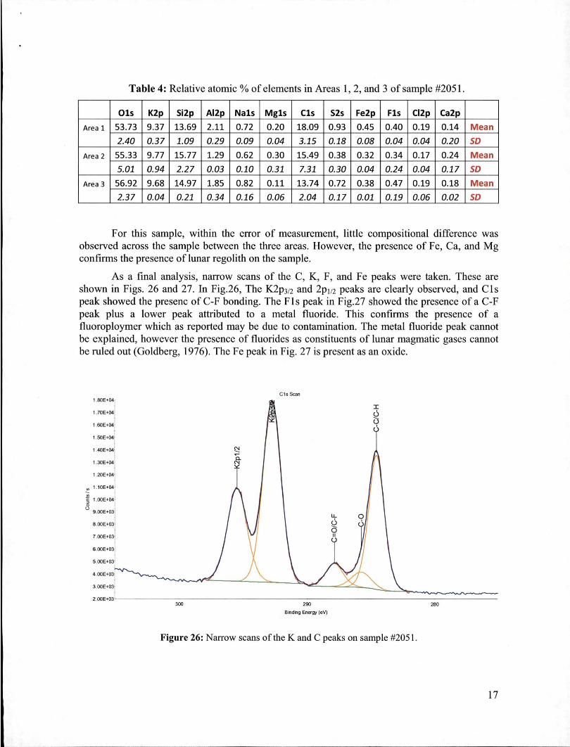
Table 4: Relative atomic % of elements in Areas 1, 2, and 3 of sample #2051.

Dis K2p Si2p AI2p Nals Mgls Cis S2s Fe2p Fls CI2p Ca2p

Area 1 53.73 9.37 13.69 2.11 0.72 0.20 18.09 0.93 0.45 0.40 0.19 0.14 Mean

2.40 0.37 1.09 0.29 0.09 0.04 3.15 0.18 0.08 0.04 0.04 0.20 SO

Area 2 55.33 9.77 15.77 1.29 0.62 0.30 15.49 0.38 0.32 0.34 0.17 0.24 Mean

5.01 0.94 2.27 0.03 0.10 0.31 7.31 0.30 0.04 0.24 0.04 0.17 SO

Area 3 56.92 9.68 14.97 1.85 0.82 0.11 13.74 0.72 0.38 0.47 0.19 0.18 Mean

2.37 0.04 0.21 0.34 0.16 0.06 2.04 0.17 0.01 0.19 0.06 0.02 SO

For this sample, within the error of measurement, little compositional difference wasobserved across the sample between the three areas. However, the presence of Fe, Ca, and Mgconfirms the presence of lunar regolith on the sample.

As a final analysis, narrow scans of the C, K, F, and Fe peaks were taken. These areshown in Figs. 26 and 27. In Fig.26, The K2P3/2 and 2pl/2 peaks are clearly observed, and CIspeak showed the presenc of C-F bonding. The F1s peak in Fig.27 showed the presence of a C-Fpeak plus a lower peak attributed to a metal fluoride. This confirms the presence of afluoroploymer which as reported may be due to contamination. The metal fluoride peak cannotbe explained, however the presence of fluorides as constituents of lunar magmatic gases cannotbe ruled out (Goldberg, 1976). The Fe peak in Fig. 27 is present as an oxide.

C1s Scan1.80E+04

1.70E+04

1.80E+04

1.50E+04

1.4lJE+04

l.30E+04

2.ooE+03'----------------------------------300 290

Bnding Energy (eV)

280

Figure 26: Narrow scans of the K and C peaks on sample #2051.

17

F1sSCM1.11E+04

1.10E+04

1.09E+04

6806907007109.90E+03'-------------------------------------

740 730 720

1.02E+04

1.00E+04

1.01E+04

Illnding E""'1lY (oV)

Figure 27: Narrow scans of the Fe and F peaks on sample #2051.

CONCLUSIO S

Computational work to determine the influence of the Apollo 12 flyby on Surveyor III isdiscussed. Saltation velocity threshold formulas (Sagan, 1990) have been implemented inMathematica and FORTRAN and compared to the gas saltation velocity computed from theFluent CFD (Dr. Xiaoyi Li - ORC). Sagan (1990) predicts interparticle cohesion forces on theorder ofnano Newtons for particles in the range of 10 to 100 /lm while Walton (2008) predicts acohesion force about 1000 times larger. Even for the small Sagan cohesion force, particles arenot predicted to make it to the Surveyor III site at R = 109 m. The results of these simulationsare summarized as follows:

(1) Particles less than 13 /lm diameter D can be ejected the full distance from the LM groundtrack to the Surveyor III site (a minimum distance of 109 m).

(2) Particles in the size range of 17 /lm < D < 2600 /lm can be lifted by the gas shear stress,based on the h = 45 m case from Xiaoyi.

(3) Even in the h = 45 m case, (1) and (2) above do not overlap, so that no particles will beejected the full 109 m to the Surveyor site.

The actual nozzle height is 67 m, but we only have the simulations for h = 25 and 45 m. Basedon a rough extrapolation estimate, no particles will be lifted for the h = 67 m case. However, it isbelieved that secondary collisions of larger particles with the surface soil may likely lead tosmaller particles being ejected and impacting the Surveyor, possible coating it with a layer offine dust.

Computational work also done to model of the soil pressurization during a lunar landing and theoutgasing from the soil after the engines are shut down. The time taken to significantly off-gas

18

the soil was predicted for various conditions and range of parameter values. This was comparedto the observed dust settling time (~30 seconds) obtained from the Apollo landing videos. Thesesimulations show that the time constant associated with the outgasing is consistent with theoptical opacity decay seen in the Apollo videos.

X-ray Photoelectron Spectroscopy (XPS) measurements of Surveyor III samples have beenperformed on coupons which either faced towards or away from the Apollo 12 LM. A 30 micronX-ray spot size was used to analyze embedded particles for compositional differences. The XPSdata were compared to Apollo 12 data from the Lunar and Planetary Institute. X-rayPhotoelectron Spectroscopy (XPS) measurements of Surveyor III samples were performed.Multiple spots along darkened and lighter regions of the samples have been measured, and thechemical compositions were correlated. The XPS data taken on samples from the Surveyor IIIcamera housing show the presence of lunar regolith. The concentration of elements comprisingthe lunar regolith were determined to be in higher concentrations in the darker areas of thesamples #2048 and #2050.

ACKNOWLEDGEMENTS

The authors would like to thank Dr. Stephen Perusich for providing the historical backgroundand organizing the original project report, "Surveyor III / Apollo 12 Particle and ChargeDynamics", ASRC Final Task Order Report, December 31, 2010.

REFERENCES

Aronowitz, L., "Electrostatic Potential Generated by Rockets on Vehicles in Space," IEEE Trans. ElectromagneticCompatibility, EMC-10, 341 (1968).

Carroll, W. F., P. M. Blair, "Discoloration and Lunar Dust Contamination of Surveyor III Surfaces," Proc. SecondLunar Sci. Con!, 3, 2735 (1971).

Colwell, 1. E. , S. R. Robertson, M. Honinyi, X. Wang, A. Poppe, and P. Wheeler, "Llmar Dust Levitation," J.Aerospace Eng., January, 2 (2009).

Eskin, D., S. Voropayev, "An Engineering Model of Particulate Friction in Accelerating Nozzles," Powder Tech.,145,203 (2004).

Goldberg, R.H., R.A. Weller, T.A. Tombrello, & D.S. Burnett, "Surface concentrations of F, H, and C", Lunar andPlanetary Science Conf., Vol. 7, p.307, 1976

Heiken, G.H., D.T. Vaniman, B.M. French Lunar Sourcebook; A user's guide to the moon, Eds., Lunar andPlanetary Institute, 1991.

[mmer, c., P. Metzger, P. Hintze. A. Nick, & R. Horan, "Apollo 12 lunar module exhaust plume impingement onlunar Surveyor III", doi: 10. 10 I6/j.icarus.20 10.1 1.013

Iversen, J.D, B.R. White, "Saltation Threshold on Earth, Mars, and Venus", Sedimentology, 29, 1982, pp. 111-119.

Kalman, H., A. Satran, D. Meir, and E. Rabinovich, "Pickup (Critical) Velocity of Particles," Powder Tech., 160,103 (2005).

Mazumder, M. K., P. K. Srirama, R. Sharma, A. S. Biris, I. Hidetaka, S. Trigwell, and M. N. Horenstein, "Lunar andMartian Dust Dynamics," IEEE Ind Appl. Magazine, July/Aug, 14 (2010).

Rabinovich, E., H. Kalman, "Pickup, Critical, and Wind Threshold Velocities of Particles," Powder Tech., 176,9(2007).

Sagan, c., Christopher Chyba, "Triton's Streaks as Windblown Dust," Nature, 346,1990, pp. 546-548.

19

Simoneit, B. R., A. L. Burlingame, "Organic Analyses of Selected Areas of Surveyor III recovered on the Apol1o 12Mission," Nature, 234, 210 (1971).

Trigwel1, S., D. Boucher, and C. 1. Cal1e, "Electrostatic Properties of PE and PTFE Subjected to AtmosphericPressure Plasma Treatment; Correlation of Experimental Results with Atomistic Modeling," J Electrostatics,65, 401 (2007).

Walton, O.R., "Review of Adhesion Fundamentals for Micron-Scale Particles", Powder and Particle Journal, 26,2008, pp. 129-141.

20