Embed Size (px)
Citation preview

1
Fusion of Probabilistic A* Algorithm and Fuzzy Inference System for Robotic Path Planning
Rahul Kala*
MTech 0091-9993746487
http://students.iiitm.ac.in/~ipg_
200545/
Anupam Shukla
Associate Professor 0091-751-2448822
http://faculty.iiitm.ac.in/~anup
amshukla/
Ritu Tiwari
Assistant Professor 0091-751-2448822
http://faculty.iiitm.ac.in/~rituti
wari/
Indian Institute of Information Technology and Management Gwalior, Gwalior, MP, INDIA
* Corresponding Author:
Citation: R. Kala, A. Shukla, R. Tiwari (2010) Fusion of probabilistic A* algorithm and fuzzy inference system
for robotic path planning, Artificial Intelligence Review 33(4), 275-306.
Final Version Available At: http://link.springer.com/article/10.1007%2Fs10462-010-9157-y?LI=true
Abstract
Robotic Path planning is one of the most studied problems in the field of robotics. The problem has been solved
using numerous statistical, soft computing and other approaches. In this paper we solve the problem of robotic
path planning using a combination of A* algorithm and Fuzzy Inference. The A* algorithm does the higher level
planning by working on a lower detail map. The algorithm finds the shortest path at the same time generating
the result in a finite time. The A* algorithm is used on a probability based map. The lower level planning is
done by the Fuzzy Inference System (FIS). The FIS works on the detailed graph where the occurrence of
obstacles is precisely known. The FIS generates smoother paths catering to the non-holonomic constraints. The
results of A* algorithm serve as a guide for FIS planner. The FIS system was initially generated using heuristic
rules. Once this model was ready, the fuzzy parameters were optimized using a Genetic Algorithm. Three
sample problems were created and the quality of solutions generated by FIS was used as the fitness function of
the GA. The GA tried to optimize the distance from the closest obstacle, total path length and the sharpest turn
at any time in the journey of the robot. The resulting FIS was easily able to plan the path of the robot. We tested
the algorithm on various complex and simple paths. All paths generated were optimal in terms of path length
and smoothness. The robot was easily able to escape a variety of obstacles and reach the goal in an optimal
manner.
Keywords: Path Planning, Robotics, Fuzzy Inference System, A* Algorithm, Genetic
Algorithm, Heuristics, Probabilistic Fitness, Hierarchical Algorithms.
1. Introduction
Robotics is a highly multi-disciplinary field that incorporates inputs from wireless systems, networks, cognition,
image processing, AI, electrical, electronics and other related fields (Lima and Custodio 2005). The highly
multi-disciplinary nature makes it an exciting playground for people from various fields to collaborate and
contribute. The whole problem of robotics include taking input from sensors, making of robotic world map, path
planning, robot control (Lee and Chiu 2009), multi-robot coordination, high-end planning, etc (Ge and Lewis
2006). The application of AI and Soft Computing techniques in the recent years deserves a special mention.
Path Planning (Kavraki et al 1996) is a specific problem in case of robots where we are given a map of the
world. Through this we can come to know about the various paths and obstacles. The problem is to compute a
path for the robot that can guide it to reach a specific goal starting from a specific position. Using this path the
robot can reach its goal without colliding from any of the obstacles. The problem is usually studied under two
separate headings. These are path planning in a static environment and path planning in a dynamic environment.
In static environment the obstacles are static and do not change their position w.r.t. time. On the other hand, in

2
dynamic path planning the position of obstacles may change with time. A path planning algorithm must ensure
that if a solution is possible, it is found and returned. This is called the completeness of the algorithm (Bohlin
and Kavraki 2000). It must also ensure that the algorithm gives its result within the specified amount of time
(Kala et al 2009).
The problem of path planning takes its input a map. A robotic map is a representation of the world of the robot
(Lozano and Wessley 1979). The map depicts the traversable path, obstacles, surface and conveys other
information. Various types of paths may be drawn depending upon the problem and solution requirements.
Some of the commonly used maps include topological maps (Thrun 1998), Voronoi maps (Castejon et al 2005;
Sud 2008), hybrid maps, etc. The map is built using the results of the various sensors along with the output of
the recognition systems (Ge and Lewis 2006).
Path planning usually provides output to the robotic control. This consists of a controller which is supposed to
move the robot in the desired path. Various robot controllers have been designed. Some of them are built using
the Adaptive Neuro-Fuzzy architecture (Ng and Trivedi 1998).
It was earlier shown by the authors that A* generates good results for the problem of path planning (Shukla,
Tiwari and Kala 2008). However, the algorithm was found to be computationally very expensive. The A*
algorithm also generates very sharp paths which the real robot would find it very difficult to follow. These are
called the non-holonomic constraints of the robot. The motivation behind this work is to adapt A* algorithm to
cater to these constraints. We do this with the application of probability based map representation
(Kambhampati and Davis 1986).
The map in this paper has been modeled in a similar way to the quad tree approach as used by Kambhampati
and Davis (1986). Here the top the nodes have high degree of uncertainty regarding the presence or absence of
the obstacles. This uncertainty is measured in terms of grayness of the cell. A completely white cell denotes
complete absence of obstacles from the region. On the other hand a completely black cell denotes the
conformation of presence of obstacle in the cell. Grey denotes the intermediate values with the intensity
denoting the probability of the cell being free from obstacles.
In practical problems, the map may be too large for the standard A* algorithm to solve. This problem is solved
by making a hierarchical solution to the problem. The A* algorithm works on this probability based map. It tries
to find a path of the smallest length that has a high probability of non-collision. The high probability factor
ensures that it is feasible to follow this path and reach the goal without colliding with the obstacles. The path
length factor ensures that the path generated is optimal to a good extent.
The A* algorithm gives the basic structure of the solution on a low level detailed map. This solution acts as a
guide for the Fuzzy Inference System (FIS) based planner. The FIS planner generates solution in less time. The
solutions follow the non-holonomic constraints. Also the solutions generated by the FIS avoid the robot getting
too close to the obstacle. This is analogous to the motion of vehicles in everyday life. The FIS solution works on
the detailed map and the solution generated by them is the final solution.
The initial fuzzy model used by the system was developed by experimentation and best of the understanding of
the problem. Once this basic prototype was ready, GA was used to further optimize the model. There were 3
basic maps of ranging complexities that were used by the GA as benchmark problems. The GA was supposed to
optimize the performance w.r.t. these maps. The performance was measured in terms of total path length,
distance from nearest obstacle and the maximum turn angle. It may be seen that any good path would have the
least length of the total path length, comfortable distance from nearest obstacle and least maximum turn angle at
any time in the run on the path. GA fine tunes the generated model to convert it into the model that can be used
for any general case.
The problem of path planning has been a very active area of research. The problem has seen numerous methods
and means that cater to the needs of the problems. A class of algorithms uses the potential method approach to
navigate a robot (Ge and Lewis 2006). In this approach, whenever the robot collides with a robot, a large
potential is given. The potential increases if the robot moves too close to the obstacle. The aim is the
minimization of the potential.
Pozna (2009) solved the problem using a potential field approach for obstacle avoidance. Other potential field
methods include (Tsai and Chuang 2001). Hui and Pratihar (2009) gave a comparison between the Potential
Field and the Soft Computing solutions. Various statistical approaches have also been used. This includes the

3
work of Jolly, Kumar and Vijaykumar who used Bezier Curve for path planning (2009). Goel (1994) solved the
problem for dynamic obstacles using an adaptive strategy. Quad Tree (Kambhampati 1986), Mesh (Hwang et al
2003), Pyramid (Urdiales et al 1998) are representations that have been tried for better performance.
Considerable work exists using the Soft Computing approaches especially Genetic Algorithms (Alvares, Caiti
and Onken 2004; Juidette and Youlal 2000; Xiao, Michalewicz, and Zhang 1997; Lin, Michalewicz and Zhang
1994), A* Algorithms (Shukla, Kala and Tiwari 2008) and Artificial Neural Networks (Kala et al 2009).
Shibata, Fukuda and Tanie (1993) used Fuzzy Logic for fitness evaluation of the paths generated. Various other
approaches (Ordonez et al 2008; Cortes, Jaillet and Simeon 2008) have also been proposed.
Zhu and Latombe (1991) used the concepts of cell decomposition and hierarchal planning. Here they
represented the cells in a similar concept of grayness denoting the obstacles. Urdylis et al (1998) used a multi-
level probability based pyramid for solving the path planning problem. Hierarchical Planning can also be found
in the work of Lai, Gen and Mamun (2007) and Shibata, Fukuda and Tanie (1993).
Along with the problem of path planning, the researchers have also studied the degrees of freedom and
dimensionality as they have a deep impact on the solution. Jan, Chang and Parberry (2008) presented their work
for solving in 3 degrees of freedom.
Chen and Chiang (2003) made an adaptive intelligent system and implemented it using a Neuro-Fuzzy
Controller and Performance Evaluator. Their system explored new actions using GA and generated new rules. In
the field of multi-robot systems, Carpin and Pagello (2009) used an approximation algorithm to solve the
problem of robotic coordination using the space-time data structures. They showed a compromise between
speed and quality. Pradhan, Parhi and Panda (2009) solved a similar problem for unknown environments using
Fuzzy Logic. Peasgood, Clark and McPhee (2008) solved the multi-robot planning problem ensuring
completeness using Spanning Trees. Hazon and Kaminka (2008) analyzed the completeness of the multi-robot
coverage problem.
This paper is organized as follows. Section 2 gives the picture of the algorithm along with the discussion on
hierarchical maps. The FIS planner is discussed in section 3. In section 4 we discuss the A* algorithm. Section 5
talks about the Genetic Optimizations. In section 6 we discuss the simulation model and the results. Section 7
gives the conclusions.
2. Algorithm Outline
In this section we give a general outline to the algorithm that we have developed for solving the problem of
robotic path planning. The basic methodology is to use the A* algorithm for a higher end planning and FIS for
the lower end planning. The FIS model is optimized by the use of GA. The general structure of the algorithm is
given in figure 1.
The algorithm starts by taking as input the initial graph. This graph may be approximately built by the map
building algorithm. This means that we do not certainly know whether obstacle lies at some cell or not
(Kambhampati and Davis 1986). The A* algorithm runs on this map to generate a path P. The path P is a
collection of points pi such that p1 is the cell cluster where the source node is found and pN is the cell cluster
where the goal node is found, N being the number of points in the A* solution.
These points are then used one after the other (other than the source) to act as guide for the Fuzzy Planner. As
soon as the robot enters the region in which the goal cell is found, the next point in P becomes the goal and the
robot has to move a step further. This goes on and on till the robot reaches the final block where the goal node is
found. The FIS is used in every block for guiding the robot. After the last iteration, a FIS planner is used to
make the robot reach the exact cell where the goal is located.
The training stage needs to be applied only once to generate the FIS. Afterwards the FIS may be used reputedly
for all problems. First the initial FIS is generated and then the FIS parameters are optimized using GA. For this
purpose benchmark maps were used. We discuss the various steps of the algorithm one by one.
2.1 Map
A map is the representation of the robotic world. The path planning algorithms use a map to get information
about the obstacles and paths that are accessible. In this paper we have used a probabilistic approach to represent

4
a map. The map is represented in the form of grids of variable sizes. Each grid is marked with a color from
white to black through grey. The color denotes the probability of the obstacles lying in that region. White means
presence of no obstacle and black means a confirmed presence of obstacle. The grids are converted into a graph
before running the A* algorithm. In the graph each vertex represents grids. All grids that are accessible by other
grids (irrespective of presence or absence of obstacles) are marked as edges. One such representation of the map
is given in figure 2.
Fig 1: The whole algorithm
Fig 2: The map at any general point of time
The grayness is the measure of the number of obstacles in the cell. The grayness of any cell c may be calculated
by using equation (1).
(1)
Suppose the whole map is built on a unit map consisting of some unit cells. The formula given by (1) in such a
case converts into (2).
(2)
Generate
Uncertain Map
Use FIS planner
using pi as goal and
add result to path
Generate initial
FIS
For all
points pi in
the solution by A* (i≥2)
Optimize FIS
parameters by
GA
P ← Path by A*
algorithm
Stop
Training
Testing Trained
FIS

5
Grayness of any cell lies between 0 and 1 and hence denotes the probability of collision of the robot in that cell.
The probability based map is used only by the A* algorithm. The FIS planner uses the grid map where each grid
is of unit size. The probability of the occurrence of obstacles in this grid is either 0 or 1.
The graph may be generated by decomposition of the probability based map. The map hence represents a two
level hierarchy. The A* algorithm runs at the first level and the FIS planner at the second level. The first level is
the abstract level and the second level is the detailed level. A graph at the first level consists of a number of
grids of the second level. Let each grid at the second level consist of α x α grids of first level, where α is a
parameter of the algorithm. If we increase α, the number of grids at the first level would decrease and vice versa.
This is shown in figure 3.
Fig 3: The 2 level hierarchy in map
2.2 The A* Guidance
The A* algorithm acts as a guide for the FIS. In this section we discuss this relation between the A* and FIS
algorithm. The A* algorithm returns a set of points pi at the first level that lead us to the goal. For the sake of
convenience, we denote any point by (xi,yi) where x and y are the coordinates of the mid-point of the region
covered by this point comprising of the level 2 points. The source is a level 2 point located somewhere in the p1
region. The algorithm first sets p2 as the goal for the robot that is still situated at the start position. The robot
moves towards p2 with an aim to reach it. As soon as the robot exits the region in which p1 is located and enters
into the region where p2 is located, the goal is changed to p3. Now the robot tries to move towards p3. The robot
keeps moving in this manner. In general if it is at any point of time at some region (xi,yi) covered by pi, it would
have as its goal the point pi+1. This mechanism of guiding the robot goes on till the robot enters the region of pN.
Now the actual goal guides the robot to complete the left journey. The concept of the level 1 and level 2 points
is shown in figure 4.
Figure 5 shows the robotic guidance. The red line shows the solution generated by the A* algorithm. Here the
robot starts from the source with the goal as P2. While it is at area P3, the goal is P4. As soon as the robot
reaches the point A, the goal is changed to P5. This way the robot keeps moving.
3 Fuzzy Inference System Planner
The movement of the robot in the system is done by a FIS Planner. The initial FIS was generated by hit and trial
method. The FIS is supposed to guide the robot to reach the goal position. The FIS tries to find out the most
optimal next move of the robot.
Map
Level 1
Level 2

6
Fig 4: The formation of layer 2 grid from layer 1 points
Fig 5: The robotic guidance
3.1 Inputs and Outputs
The FIS takes 4 inputs. There are angle to goal (α), distance from goal (dg), distance from obstacle (do) and turn
to avoid obstacle (to).
The angle to goal is the angle (α, measured along with sign) that the robot must turn in order to face the goal.
This is measured by taking the difference in current angle of the obstacle (φ) and the angle of the robot (θ). The
result is always between -180 degrees and 180 degrees. This is shown in figure 6.
The distance from goal (dg) is the distance between the robot and the goal position. This distance is normalized
to lie between 0 and 1 by multiplying by a constant. Similarly the distance from obstacle (do) is the distance
between the robot and the nearest obstacle found in the direction in which the robot is currently moving. This is
also normalized to lie between 0 and 1.
The turn to avoid obstacle angle (to) is a discrete input that is either ‘left’, ‘no’ or ‘right’. These stand for
counter-clockwise turn, no turn and clockwise turn respectively. This parameter represents the turn that the
robot must make in order to avoid the closest obstacle. This input is measured by measuring the distance
between the robot and the obstacle at three different angles. The first distance is the distance between the
obstacle and the robot measured at the angle at which the robot is facing (a). The second distance is the same
distance measured at an angle of dθ more (c). The third distance is measured at an angle dθ less (b). These three
distances are given in figure 7.
(xi,yi)
(xi,yi+b)
(xi+a,yi+b)
(xi+a,yi)
(xi+a/2,yi+b/2)

7
Figure 6: The angle to goal
Fig 7: The determination of turn to avoid obstacle
Various cases are now possible. The first case is c>b. This means that the obstacle was turned in such a way that
turning in the clockwise direction made it even further. In this case the preferred turn is clockwise with an
output of ‘right’. The second case is b>c. This means that the obstacle was turned in such a way that turning in
the anti-clockwise direction made it even furtherer. In this case the preferred turn is anti-clockwise with an
output of ‘left’. The third case is b=c. This is the case when the robot is vertically ahead of the robot. In such a
case we follow a ‘left preferred’ rule and take a ‘left’ turn.
There is a single output that measures the angle (β) that the robot should turn, along with direction. The
membership functions of the different inputs and outputs are given in figure 8.
3.2 Rules
Rules are the driving force for the FIS. Based on the inputs, we frame rules for the FIS to follow. The rules
relate the inputs to the outputs. Each rule has a weight attached to it. Further some inputs have been applied with
the not operator as well. All this makes it possible to frame the rules based on the system understanding.
The rules can be classified into two major categories. The first category of rules tries to drive the robot towards
the goal. The second category of rules tries to save the robot from obstacles. If an obstacle is very near, the
Goal
θ φ
α= θ- φ
c
a
Obstacle
Robot
b

8
second category of rules become very dominant. 11 rules are identified. These are given in figure 9. The
numbers in brackets denote the weights.
(a) Angle to goal (b) Distance to goal
(c) Distance from obstacle (d) Turn to avoid obstacle
(e) Turn (Output)
Fig 8: The membership functions
Fig 9: The FIS rules
Rule1: If (α is less_positive) and (do is not near) then (β is less_right) (1)
Rule2: If (α is zero) and (do is not near) then (β is no_turn) (1)
Rule3: If (α is less_negative) and (do is not near) then (β is less_left) (1)
Rule4: If (α is more_positive) and (do is not near) then (β is more_right) (1)
Rule5: If (α is more_negative) and (do is not near) then (β is more_left) (1)
Rule6: If (do is near) and (to is left) then (β is more_right) (1)
Rule7: If (do is near) and (to is right) then (β is more_left) (1)
Rule8: If (do is far) and (to is left) then (β is less_right) (1)
Rule9: If (do is far) and (to is right) then (β is less_left) (1)
Rule10: If (α is more_positive) and (do is near) and (to is no_turn) then (β is less_right) (0.5)
Rule11: If (α is more_negative) and (do is near) and (to is no_turn) then (β is less_left) (0.5)
9
4 A* Algorithm
The A* algorithm is responsible for the high end planning of the robot. A* algorithm generates very efficient
solutions in robotic path planning problem. In this algorithm, we have used a probability based A* algorithm.
The reason for this is that the A* algorithm runs at a level, where the exact information about the obstacles is
unknown. The A* algorithm tries to find a solution in this probability based map. The algorithm is supposed to
minimize the path length and at the same time maximize the probability of reaching the goal from this path.
The A* uses the cost function for deciding the goodness of the solution. The better solutions have lower costs.
Hence the approach is generally to find smaller costs and expand the associated nodes further. This algorithm is
based on probability that is denoted by the probability of finding obstacle in the cell. Hence each path we
traverse has some probability of success associated with it. This probability for a path is given by equation (3).
(3)
Here pi are the consecutive nodes that make up the total path P.
The other costs that the algorithm uses are Heuristic Cost h(n) and the Historical Cost g(n). For the A*, the total
cost f(n) is given by the sum of Heuristic Cost h(n) and Historical Cost g(n). In this algorithm we use the historic
cost as distance of the center of the node from the source and the heuristic cost as the cost of the center of node
to the goal.
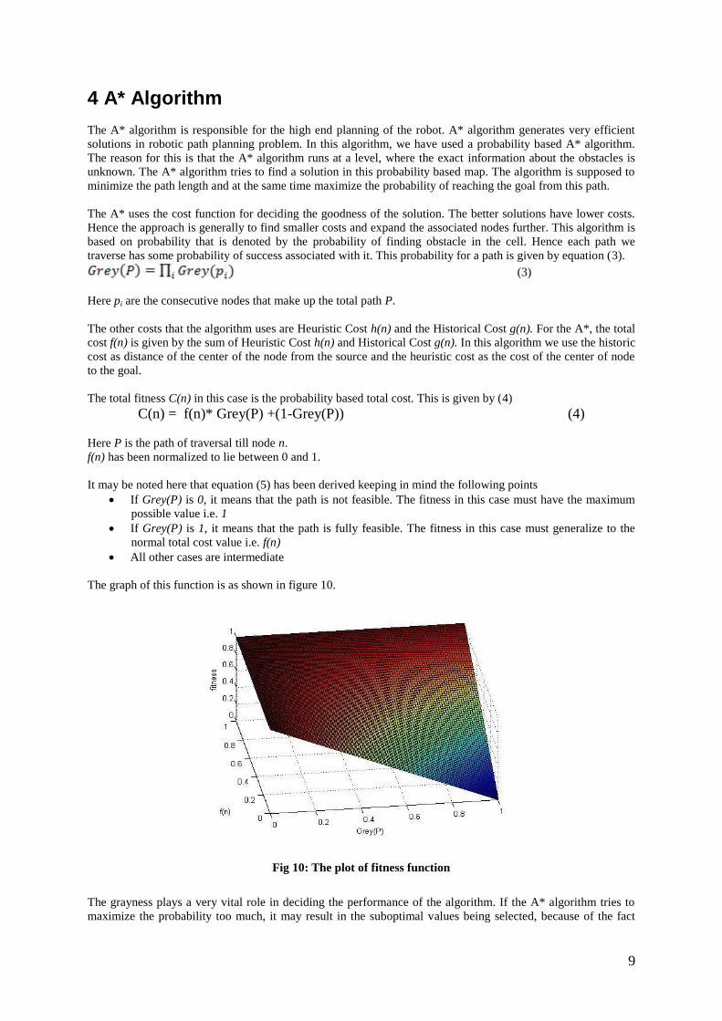
The total fitness C(n) in this case is the probability based total cost. This is given by (4)
C(n) = f(n)* Grey(P) +(1-Grey(P)) (4)
Here P is the path of traversal till node n.
f(n) has been normalized to lie between 0 and 1.
It may be noted here that equation (5) has been derived keeping in mind the following points
If Grey(P) is 0, it means that the path is not feasible. The fitness in this case must have the maximum
possible value i.e. 1
If Grey(P) is 1, it means that the path is fully feasible. The fitness in this case must generalize to the
normal total cost value i.e. f(n)
All other cases are intermediate
The graph of this function is as shown in figure 10.
Fig 10: The plot of fitness function
The grayness plays a very vital role in deciding the performance of the algorithm. If the A* algorithm tries to
maximize the probability too much, it may result in the suboptimal values being selected, because of the fact

10
they lead to higher probability. This would result in the robot opting for longer paths to avoid any possible
obstacle. Based on these ideas, we try to modify equation (5) by introducing a parameter β that controls the
effect of the grayness in the fitness function. If the value of β is kept as 0, the A* algorithm completely discards
the effect of grayness and converts into a normal un-probabilistic A* algorithm. The modified equation (4) is
given by equation (5).
C(n) = f(n)* Grey’(P) +(1-Grey`(P)) (5)
Here Grey`(P) is given by equation (6)
Grey`(P) = 1, if Grey(P) > β
Grey(P) otherwise (6)
The fitness function for β=0.6 is given in figure 11
.
Fig 11: The plot of modified fitness function
5 Genetic Optimizations
The Fuzzy model discussed in section 3 was an initial fuzzy model that was generated. The parameters of this
model were decided by trial and error. In order to make this a scalable system, further optimizations were
necessary. This was done by means of GA. GA was supposed to optimize the fuzzy parameters (parameters of
all membership functions used) for most optimal planning of the robotic path. There were a total of 32 fuzzy
parameters that were optimized by the GA.
For this problem, we first created 3 maps that acted as benchmark maps for the GA. The GA was supposed to
optimize the performance of the system against these maps. The first map was a simple map with no obstacles.
The second map had single obstacles on the way from source to goal. The robot was supposed to avoid this path.
The third map had many obstacles and the robot was supposed to find its way out of them. These maps are given
in figure 12.
Fig 12: Benchmark maps for GA (a) No obstacle (b) Single obstacle (c) Many Obstacles

11
The fitness function for any of the map i tried to optimize three objectives (i) The total path length (Li) (ii) The
maximum turn taken any time in the path (Ti) (iii) Distance from the closest obstacle anytime in the run (Oi). All
these were normalized to lie on a scale of 0 to 1. The total fitness for any map i may hence be given by (7)
Fi = Li * (1-Oi) * Ti (7)
The fitness Fi for any solution hence lies between 0 and 1. 1 is the maximum fitness a solution can attain. If the
robot at any time moves out of the map, or collides with an obstacle, we assign it a fitness value of 1. The GA
would naturally result in deletion of such solutions in the course of generations. In this manner we handle
infeasible solutions in GA.
The total fitness (F) of any individual in GA is the sum of its score or fitness in all these three maps. This is
given by (8). The total fitness can be anywhere between 0 and 3.
F = F1 + F2 + F3 (8)
6 Simulation and Results
In order to test the working of the algorithm, we made a simulation engine of ourselves. Every attempt was
made to ensure that the simulation engine behaves in a way similar to actual robot. This would ensure that the
algorithm can be easily deployed on a real robot for the purpose of path planning. All simulations were done on
a 2.0 GHz dual core system with 1 GB RAM. The initial graph was taken as an input in form of an image. The
image depicted the obstacles as black regions and the path as the white region.
The first major task was the Genetic Optimization of the FIS. Then this optimized model was implemented and
tried on the benchmark problems. The system was then tried on numerous maps with varying obstacles. These
are given in the next sub-sections.
6.1 Genetic Optimizations
The purpose of the GA was to find out the exact parameter values for the FIS. 32 such parameters were
identified that needed optimizations. The Matlab GA toolkit was applied for the optimization purposes. The GA
search space consisted of the region around the value chosen by the hit and trial method of the 32 parameters.
We restricted the search to 10% of this value on both sides. This means if the value of any parameter was x, the
GA was supposed to optimize it in the search region of x-0.1*L to x+0.1*L where L is the total range of values
that x can take. It is natural that on the basis of rules framed, the solution was not likely to be present in any
other region. This provided ample of space for GA to locate the global minima and at the same time making the
space finite to search for possible solutions.
The population was represented by the double vector mechanism. The population size was fixed to 50. Rank
based fitness scaling was used. Stochastic Uniform selection was used. The crossover rate was 0.8 with elite
count as 2. Gaussian Mutation function was used with a scale and spread of 1 each. The GA was made to run
over 100 generations. It took about 1 hr 15 mins for the GA to complete the generations. The fitness curve of
GA showing the mean and best fitness is given in figure 13. The final fitness of 0.04850 was achieved by the
GA.
6.2 Benchmark Maps
The first tests were applied at the benchmark problems. This was an attempt to see the behavior of the algorithm
at the benchmark problems. Since these benchmark problems were applied on low resolution graph of size
100X100, there was no need to run the A* algorithm. Direct FIS planner was used. The maps are shown in
figure 12. The path traced by the algorithm after optimization is given in figure 14. Figure 15 shows the same
problem being solved by application of A* algorithm alone. In all cases the source is the top left corner of the
map and the goal is the bottom right corner of the map.
The solutions generated by the algorithm were all smooth so that the robot can be easily turned as per
requirements. They were all of optimal length. In each case the robot was easily able to steer its way by
avoiding obstacles and reach the goal node.

12
In all the cases the robot was initially facing at the direction of the X-axis and not towards the goal. This is the
reason why we see a smooth transition in path and angle at the starting points in the graph. The solutions
generated by A* algorithm however do not reveal this. These solutions assume the robot would somehow turn
towards the angle of the goal and then it would start moving in a straight line towards it.
Fig 13: The mean and best fitness in GA
(a) Map 1 (b) Map 2 (c) Map 3
Fig 14: The path traced by algorithm for benchmark maps
(a) Map 1 (b) Map 2 (c) Map 3
Fig 15: The path traced by standard A* algorithm for benchmark maps
Figure 14(b) shows another very interesting solution; where the robot made a smooth transition and started
moving in a manner to just avoid the obstacle. When the obstacle ended, it again smoothly changed its direction.
The nearness of the obstacle avoided the undue long tracing of path and the turns were smooth enough for the
robot to be taken. Similar inferences may be made from figure 14(c).
The very sharp turns present in figure 15(b) and 15(c) clearly show that these solutions are not practical and
further they cannot be easily converted to smoother paths as well. This exposes the weaknesses of A* algorithm.
Further looking at figure 14(c) and 15(c), we see that our algorithm guided the robot from the top of the obstacle
(remember we adopted a ‘left preferred’ approach). The A* algorithm on the contrary guided the robot from the
13
middle of obstacle. It may be argued that the unequal length may not be optimal. We will see later that the
guidance by the A* is responsible for the path length and it divides the problem in such a way that the most
optimal path is selected in most of the cases.
6.3 More Maps
In order to fully test the behavior of the algorithm, we tested the algorithm against 3 more maps. This time the
maps were of larger size of 1000X1000. Many obstacles were places in between the source and the goal. The
robot was supposed to reach the goal from the source. The top left corner is the source and bottom left corner is
the goal. In all the cases, the source was fixed as the top left corner and the goal was fixed as the bottom right
corner.
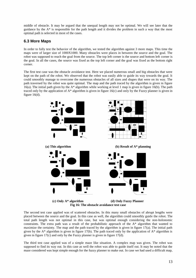
The first test case was the obstacle avoidance test. Here we placed numerous small and big obstacles that were
kept on the path of the robot. We observed that the robot was easily able to guide its way towards the goal. It
could smoothly manage to overcome the numerous obstacles of all sizes and shapes that were on its way. The
path traversed by the robot was quite optimal. The map and the path traced by the algorithm is given in figure
16(a). The initial path given by the A* algorithm while working at level 1 map is given in figure 16(b). The path
traced only by the application of A* algorithm is given in figure 16(c) and only by the Fuzzy planner is given in
figure 16(d).
(a) This algorithm (b) Result of A* planning
(c) Only A* algorithm (d) Only Fuzzy Planner
Fig 16: The obstacle avoidance test case
The second test case applied was of scattered obstacles. In this many small obstacles of abrupt lengths were
placed between the source and the goal. In this case as well, the algorithm could smoothly guide the robot. The
total path length was not optimal in this case, but was optimal enough considering the non-holonomic
constraints. The extra path was a result of the probabilistic approach of the A* algorithm that wanted to
maximize the certainty. The map and the path traced by the algorithm is given in figure 17(a). The initial path
given by the A* algorithm is given in figure 17(b). The path traced only by the application of A* algorithm is
given in figure 17(c) and only by the Fuzzy planner is given in figure 17(d).
The third test case applied was of a simple maze like situation. A complex map was given. The robot was
supposed to find its way out. In this case as well the robot was able to guide itself out. It may be noted that the
maze considered was kept simple enough for the fuzzy planner to make out. In case we had used a difficult map,

14
the fuzzy planner would have ended up in a collision. The map and the path traced by the algorithm is given in
figure 18(a). The initial path given by the A* algorithm is given in figure 18(b). Here also it tried to maximize
the probability. The path traced only by the application of A* algorithm is given in figure 18(c) and only by the
Fuzzy planner is given in figure 18(d).
(a) This algorithm (b) Result of A* planning
(c) Only A* algorithm (d) Only Fuzzy Planner
Fig 17: The scattered obstacle test case
6.4 Effect of Change in Grid Size
In this problem we had introduced a 2 level hierarchical map. The 2nd
level map was a detailed version of the 1st
level map. The 1st level was probabilistic in nature. Here various nodes of level 2 had been clubbed to form a
single grid or cell. The size of this grid (α) decides the working of the algorithm. If α is very small almost entire
graph would be available at the 1st level. The solution would be predominantly A* in nature. If the size is too
large, there would be nothing considerable at the 1st level. In that case the solution would be predominantly of
the nature of Fuzzy Planner. In all other cases, the solution would be a mixture of A* and Fuzzy planner
characteristics.
The probability based fitness used in the A* algorithm is the other factor that changes with the change of α. As
we increase α, the probability keeps getting vague due to the higher grid size. The A* algorithm tries to find
paths that have high probability of reaching to the goal. This in turn ensures that under any circumstances, the
fuzzy planner would be able to reach the goal position with the maximum level of certainty. However, the
probability has an undue effect on the path length. In order to increase the path probability, the length is
compromised. This in turn causes the total path length traversed by the robot to increase.
We studied this effect into the various maps that we had used. The path traced by the robot for one such map is
given in figure 19.

15
(a) This algorithm (b) Result of A* planning
(c) Only A* algorithm (d) Only Fuzzy Planner
Fig 18: The simple maze test case
(a) α = 1000 (b) α = 100 (c) α = 20
(e) α = 10 (f) α = 5 (c) α = 1
Fig 19: The path traced by robot for various values of α

16
6.5 Effect of Change of Grayness Parameter
The other parameter that we try to change is β. This parameter was discussed in Section 4. As per the discussion
it is clear as this parameter would increase, the conventional non-probabilistic behavior would get predominant
in the behavior of the algorithm. We studied the change of this parameter into numerous maps. Figure 20 shows
the results on the same graph that was used in our discussion in section 6.4. It may be seen that the algorithm
failed for β=0. This is because the A* algorithm returned a straight path from source to goal which had very less
probability. The other inputs could not produce a change in the output of the A* algorithm. It may be observed
here that change of β tries to make a change in A* algorithm result. As a result, the change in path would be
discrete rather than continuous. Whenever there is a change in path of the A* algorithm result, a discrete change
is reflected. This depends upon the probability conversion and the grid size (α). The experiments were
conducted at a large grid size. In smaller grids the change appears to be more continuous.
(a) β = 0 (b) β = 0.2 (c) β = 0.3
(d) β = 0.5 (e) β = 0.6 (f) β = 1
Fig 20: The path traced by robot for various values of β
6.6 Discussion of interaction between parameters:
It may easily be seen that the total path is affected by 3 factors (i) the contribution of the Fuzzy Planner that
makes the path smooth at the same time reducing time of algorithm. It however may result in a longer path or
the failure in finding path in case of complex maps (ii) the contribution of the A* algorithm in reducing the path
length (α), which can solve very complex maps with most optimal path length at the cost of computational time
(iii) The contribution of the A* to maximize the probability of the path (β), which usually would increase the
path length.
The combined effect of the change in values of α and β would reveal the generation of unique paths. This makes
the task of planning using the proposed algorithm very flexible, where different parameters may be set as per the
problem. These would result in different kinds of paths with varying path lengths and smoothness. Based on the
results of figure 16 and 17, it may be seen that we can generate all kinds of paths between A* algorithm, Fuzzy
planner and probability based approach by the adjustment of these parameters. The flexibility however puts the
constraint that these parameters need to be judiciously set, so as to attain optimal results. The parameters have a
strong dependence on numerous factors like map, path simplicity, robot design, total map size, etc. This
eliminates the possibility of constant values of these parameters for different scenarios and maps. The task of
parameter setting for α and β may be done by considering the same factors. Very simple maps with fewer turns

17
may have more A* contribution. The presence of multiple objects in the optimal path may require a lot of Fuzzy
planning to escape from the variety of objects.
7 Conclusions
In this paper we have proposed a method to solve the problem of path planning using a combination of the A*
algorithm and Fuzzy Planning. We tested the algorithm for various test cases. In all the test cases we observed
that the algorithm was able to find the correct solution. The solutions generated by the algorithm were often
close to optimal. They took relatively small times to solve for each of the map presented. Further, the solutions
obeyed the non-holonomic constraints and the path generated by the algorithm can be easily used by any robotic
controller to move the robot physically. In this paper we had further used a probabilistic approach in the map
representation. The map was implemented at two levels for the A* algorithm and the fuzzy planner. The FIS
was genetically optimized for performance.
The results convey a very unique relation between the working of the A* algorithm and the FIS planner. The A*
algorithm works over a probabilistic map trying to optimize the path length and at the same time making the
probability of reaching the goal high. The FIS was used primarily for giving smooth paths according to the non-
holonomic constraints and ensuring a timely response to the system. The A* algorithm at one hand reduced the
total path length by selecting the solutions that have less total length. At the same time the increase of
probability resulted in selection of longer paths at some positions.
We further solved each of the path with all three algorithms (i) this algorithm (ii) only A* algorithm and (iii)
only fuzzy planner. From these results it may be seen that this algorithm is a unique mix of the other two
algorithms. It tries to combine the best features of path length and smoothness in the solution it generates.
The contribution of each of the A* algorithm and Fuzzy Planner may be varied by changing the grid size (α) and
the probability factor (β). This would make the algorithm behave more like one or the other. If the grid size is
very small, the algorithm would be primarily A* in nature. This may induce very sharp paths. Further if the grid
size is very large, the resulting algorithm would be dominated by the Fuzzy planner properties. It may not be
able to solve complex maze like paths. Similarly if β is very large, the total path length might be more due to the
effort of A* to optimize the path length. Reducing β may result in shorter paths, but at the same time the robot
may fail to reach the goal or may get obstructed from the path as the path it is trying to follow may have low
probability.
Another characteristic feature is the dynamic nature of the algorithm. The Fuzzy Planner can run in a very
dynamic environment. Any change in the graph at any time can be easily adapted in real times. This further
makes it possible to use the algorithm in dynamic environments.
In the proposed algorithm GA was used to optimize the parameters of the FIS. This led to a better performance
of the FIS in escaping the obstacles and moving towards the goal. FIS represents the robotic behavior that is not
map-specific. The GA tunes the behavior in such a manner that the robot learns to take optimal moves in
different kinds of scenarios. This results in optimal movement of the robot in different kinds of map with simple
or complex-shaped obstacles.
The experimentation done in this paper was mainly on static environment. The algorithm may be further adapted
for modeling mobile obstacles in a space time graph. This would make an effective dynamic algorithm. A
further work to decide effective grid size (α) and probability factor (β) needs to be done. Formulation of more
benchmark problems covering all cases that a robot may face in real life may also be done. Further the FIS rules
may be more intensively studied and modified in the future. The algorithm is yet to be studied in a way that
balances or tunes the effects of probability of the path, the A* algorithm and the fuzzy planner in the entire path.
References [1] Alvarez A, Caiti A, Onken R (2004) Evolutionary Path Planning for Autonomous Underwater Vehicles in a
Variable Ocean , IEEE Journal of Oceanic Engineering, Vol. 29, No. 2, pp 418-429
[2] Bohlin R, Kavraki L E (2000) Path planning using lazy PRM , Proceedings. IEEE International Robotics
and Automation ICRA '00, Vol: 1, pp: 521-528, San Francisco, CA, USA
[3] Carpin S, Pagello E (2009) An experimental study of distributed robot coordination , Robotics and
Autonomous Systems, Volume 57 , Issue 2, pp 129-133

18
[4] Castejon C, Blanco D; Boadai B L, Moreno L (2005) Voronoi-Based Outdoor Traversable Region
Modelling , Innovations in Robot Mobility and Control, Springer, pp 1-64
[5] Chen, L H, Chiang C. H. (2003) New Approach to Intelligent Control Systems With Self-Exploring Process
, IEEE Transactions on Systems, Man and Cybernetics—Part B: Cybernetics, Vol. 33, No. 1, pp 56-66
[6] Cortes J; Jaillet L, Simeon T (2008) Disassembly Path Planning for Complex Articulated Objects , IEEE
Transactions on Robotics, Vol. 24, No. 2, pp 475-481
[7] Ge S S, Lewis F L (2006) Autonomous Mobile Robot , Taylor and Francis
[8] Goel, A K (1994) Multistrategy Adaptive Path Planning , IEEE Special Feature, pp57-65
[9] Hazon N, Kaminka G A (2008) On redundancy, efficiency, and robustness in coverage for multiple robots ,
Towards Autonomous Robotic Systems 2008,Volume 56, Issue 12, pp 1102-1114
[10] Holland J H (1975) Adaptation in natural and artificial systems , Ann Arbor: University of Michigan Press
[11] Hui N B, Pratihar D K (2009) A comparative study on some navigation schemes of a real robot tackling
moving obstacles , Robotics and Computer-Integrated Manufacturing, doi:10.1016/j.rcim.2008.12.003
[12] Hwang J Y, Kim J S, Lim S S, Park K H (2003) A Fast Path Planning by Path Graph Optimization , IEEE
Transaction on Systems, Man, and Cybernetics—Part A: Systems and Humans, Vol. 33, No. 1, pp 121-128
[13] Jan G. E., Chang K Y, Parberry I (2008) Optimal Path Planning for Mobile Robot Navigation , IEEE/ASME
Transactions on Mechatronics, Vol. 13, No. 4, pp 451-460
[14] Jolly K G, Kumar R S, Vijayakumar R (2009) A Bezier curve based path planning in a multi-agent robot
soccer system without violating the acceleration limits , Robotics and Autonomous Systems, Volume 57, Issue 1,
pp 23-33
[15] Juidette H, Youlal H (2000) Fuzzy dynamic path planning using genetic algorithms , IEEE Electronics
Letters, Vol. 36 No. 4, pp 374-376
[16] Kala R et. al. (2009) Mobile Robot Navigation Control in Moving Obstacle Environment using Genetic
Algorithm, Artificial Neural Networks and A* Algorithm , Proceedings of the IEEE World Congress on
Computer Science and Information Engineering (CSIE 2009), Los Angeles/Anaheim, USA
[17] Kambhampati S, Davis L S (1986) Multiresolution Path Planning for Mobile Robots , IEEE Journal of
Robotics and Automation, Vol RA-2, No. 3, pp135-145
[18] Kavraki L E, Svestka P, Latombe J C, Overmars M H (1996) Probabilistic roadmaps for path planning in
high-dimensionalconfiguration spaces , IEEE Transactions on Robotics and Automation, Volume: 12, Issue: 4,
pp 566-580
[19] Lai X C, Ge S S, Mamun A A (2007) Hierarchical Incremental Path Planning and Situation-Dependent
Optimized Dynamic Motion Planning Considering Accelerations , IEEE Transactions on Systems, Man, and
Cybernetics—Part B: Cybernetics, Vol. 37, No. 6, pp 1541-1554
[20] Lee C H, Chiu M H (2009) Recurrent neuro fuzzy control design for tracking of mobile robots via hybrid
algorithm , Expert Systems with Applications, doi:10.1016/j.eswa.2008.11.051
[21] Lima P U, Custodio L M (2005) Multi-Robot Systems , Innovations in Robot Mobility and Control,
Springer, pp 1-64
[22] Lin H S, Xiao J, Michalewicz Z (1994) Evolutionary Algorithm for Path Planning in Mobile Robot
Environment , Proceedings of the First IEEE Conference on Evolutionary Computation (ICEC'94), pp 211-216
[23] Lozano P T, Wesley M A (1979) An algorithm for planning collision-free paths among polyhedral
obstacles , Communications of the ACM, pp 560–570.
[24] Ng K C, Trivedi M M (1998) A neuro-fuzzy controller for mobile robot navigation and
multirobotconvoying , IEEE Transactions on Systems, Man, and Cybernetics, Part B: Cybernetics, Volume: 28,
Issue: 6, ,pp 829-840
[25] O’Hara K J, Walker D B, Balch T R (2008) Physical Path Planning Using a Pervasive Embedded Network ,
IEEE Transactions on Robotics, Vol. 24, No. 3, pp 741-746
[26] Ordonez C, Collins J, Emmanuel G, Selekwa M F, Dunlap, D D (2008) The virtual wall approach to limit
cycle avoidance for unmanned ground vehicles , Robotics and Autonomous Systems, Volume 56, Issue 8, pp
645-657
[27] Peasgood M, Clark C M, McPhee J (2008) A Complete and Scalable Strategy for Coordinating Multiple
Robots Within Roadmaps , IEEE Transactions on Robotics, Vol. 24, No. 2, pp 283-292
[28] Pozna C et. al. (2009) On the design of an obstacle avoiding trajectory: Method and simulation ,
Mathematics and Computers in Simulation, doi:10.1016/j.matcom.2008.12.015
[29] Pradhan S K, Parhi D, Panda A K (2009) Fuzzy logic techniques for navigation of several mobile robots ,
Applied Soft Computing, Volume 9 , Issue 1, pp 290-304
[30] Shibata T, Fukuda T, Tanie K(1993) Fuzzy Critic for Robotic Motion Planning by Genetic Algorithm in
Hierarchical Intelligent Control , Proceedings of 1993 International Joint Conference on Neural Networks, pp
77-773
[31] Shukla A, Kala R (2008) Multi Neuron Heuristic Search , International Journal of Computer Science and
Network Security, Vol. 8, No. 6, pp 344-350

19
[32] Shukla A, Tiwari R, Kala R (2008) Mobile Robot Navigation Control in Moving Obstacle Environment
using A* Algorithm , Intelligent Systems Engineering Systems through Artificial Neural Networks, ASME
Publications, Vol. 18, pp 113-120
[33] Sud A et. al. (2008) Real-Time Path Planning in Dynamic Virtual Environments Using Multiagent
Navigation Graphs , IEEE Transactions on Visualization and Computer Graphics, Vol. 14, No. 3, pp 526-538.
[34] Thrun S (1998) Learning metric-topological maps for indoor mobile robot navigation , Artificial
Intelligence, Volume 99, Issue 1, Pages 21-71
[35] Tsai C H; Lee J S, Chuang J H (2001) Path Planning of 3-D Objects Using a New Workspace Model ,
IEEE Transactions on Systems, Man, and Cybernetics—Part C: Applications and Reviews, Vol. 31, No. 3, pp
405-410
[36] Urdiales C., Bantlera A., Arrebola F, Sandova1 F, (1998), Multi-level path planning algorithm for
autonomous robots , IEEE Electronic Letters, Vol. 34 No. 2, pp 223-224
[37] Xiao J, Michalewicz Z, Zhang L, Trojanowski K (1997) Adaptive Evolutionary Planner/Navigator for
Mobile Robots , IEEE Transactions on Evolutionary Computation, Vol. 1, No. 1, pp 18-28
[38] Zhu D, Latombe J C New Heuristic Algorithms for Efficient Hierarchical Path Planning , IEEE
Transactions on Robotics and Automation, Vol. 7, No. 1, pp 9-20