FusionFlow: Discrete-Continuous Optimization for Optical Flow Estimation

Victor LempitskyMicrosoft Research Cambridge

Stefan RothTU Darmstadt

Carsten RotherMicrosoft Research Cambridge

Abstract

Accurate estimation of optical flow is a challenging task,which often requires addressing difficult energy optimiza-tion problems. To solve them, most top-performing methodsrely on continuous optimization algorithms. The modelingaccuracy of the energy in this case is often traded for itstractability. This is in contrast to the related problem ofnarrow-baseline stereo matching, where the top-performingmethods employ powerful discrete optimization algorithmssuch as graph cuts and message-passing to optimize highlynon-convex energies.

In this paper, we demonstrate how similar non-convexenergies can be formulated and optimized discretely in thecontext of optical flow estimation. Starting with a set ofcandidate solutions that are produced by fast continuousflow estimation algorithms, the proposed method iterativelyfuses these candidate solutions by the computation of min-imum cuts on graphs. The obtained continuous-valued fu-sion result is then further improved using local gradient de-scent. Experimentally, we demonstrate that the proposedenergy is an accurate model and that the proposed discrete-continuous optimization scheme not only finds lower energysolutions than traditional discrete or continuous optimiza-tion techniques, but also leads to flow estimates that outper-form the current state-of-the-art.

1. Introduction

Optical flow has been an important area of computervision research, and despite the significant progress madesince the early works [14, 20], flow estimation has remainedchallenging to this date. Two challenges dominate recentresearch: firstly, the issue of choosing an appropriate com-putational model, and secondly, computing a good solutiongiven a particular model. Papenberg et al. [23], for example,suggested a complex continuous optimization scheme forflow estimation. Despite its success, this approach is limitedby the fact that the spatial regularity of flow is modeled asa convex function. Consequently, the estimated flow fieldsare somewhat smooth and lack very sharp discontinuitiesthat exist in the true flow field, especially at motion bound-aries. Black and Anandan [3] addressed this problem by

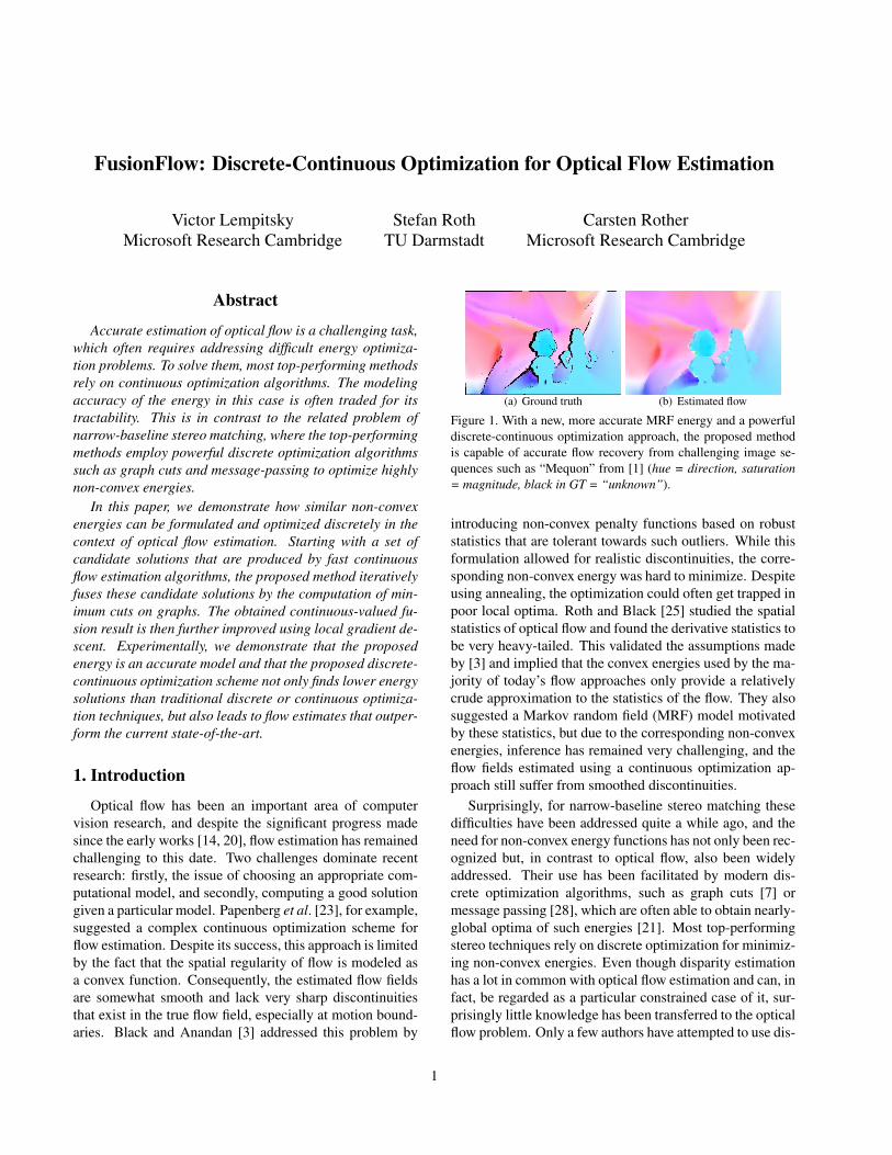
(a) Ground truth (b) Estimated flow

Figure 1. With a new, more accurate MRF energy and a powerfuldiscrete-continuous optimization approach, the proposed methodis capable of accurate flow recovery from challenging image se-quences such as “Mequon” from [1] (hue = direction, saturation= magnitude, black in GT = “unknown”).

introducing non-convex penalty functions based on robuststatistics that are tolerant towards such outliers. While thisformulation allowed for realistic discontinuities, the corre-sponding non-convex energy was hard to minimize. Despiteusing annealing, the optimization could often get trapped inpoor local optima. Roth and Black [25] studied the spatialstatistics of optical flow and found the derivative statistics tobe very heavy-tailed. This validated the assumptions madeby [3] and implied that the convex energies used by the ma-jority of today’s flow approaches only provide a relativelycrude approximation to the statistics of the flow. They alsosuggested a Markov random field (MRF) model motivatedby these statistics, but due to the corresponding non-convexenergies, inference has remained very challenging, and theflow fields estimated using a continuous optimization ap-proach still suffer from smoothed discontinuities.

Surprisingly, for narrow-baseline stereo matching thesedifficulties have been addressed quite a while ago, and theneed for non-convex energy functions has not only been rec-ognized but, in contrast to optical flow, also been widelyaddressed. Their use has been facilitated by modern dis-crete optimization algorithms, such as graph cuts [7] ormessage passing [28], which are often able to obtain nearly-global optima of such energies [21]. Most top-performingstereo techniques rely on discrete optimization for minimiz-ing non-convex energies. Even though disparity estimationhas a lot in common with optical flow estimation and can, infact, be regarded as a particular constrained case of it, sur-prisingly little knowledge has been transferred to the opticalflow problem. Only a few authors have attempted to use dis-

1

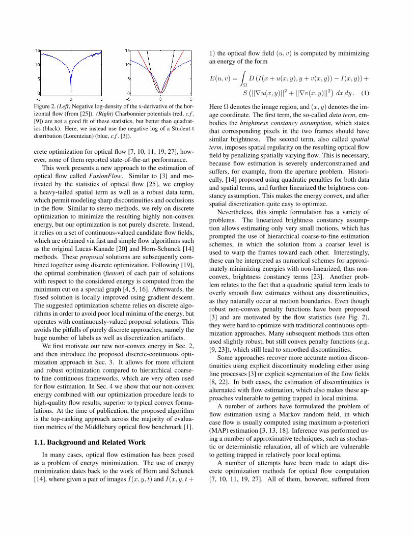
Figure 2. (Left) Negative log-density of the x-derivative of the hor-izontal flow (from [25]). (Right) Charbonnier potentials (red, c.f .[9]) are not a good fit of these statistics, but better than quadrat-ics (black). Here, we instead use the negative-log of a Student-tdistribution (Lorentzian) (blue, c.f . [3]).

crete optimization for optical flow [7, 10, 11, 19, 27], how-ever, none of them reported state-of-the-art performance.

This work presents a new approach to the estimation ofoptical flow called FusionFlow. Similar to [3] and mo-tivated by the statistics of optical flow [25], we employa heavy-tailed spatial term as well as a robust data term,which permit modeling sharp discontinuities and occlusionsin the flow. Similar to stereo methods, we rely on discreteoptimization to minimize the resulting highly non-convexenergy, but our optimization is not purely discrete. Instead,it relies on a set of continuous-valued candidate flow fields,which are obtained via fast and simple flow algorithms suchas the original Lucas-Kanade [20] and Horn-Schunck [14]methods. These proposal solutions are subsequently com-bined together using discrete optimization. Following [19],the optimal combination (fusion) of each pair of solutionswith respect to the considered energy is computed from theminimum cut on a special graph [4, 5, 16]. Afterwards, thefused solution is locally improved using gradient descent.The suggested optimization scheme relies on discrete algo-rithms in order to avoid poor local minima of the energy, butoperates with continuously-valued proposal solutions. Thisavoids the pitfalls of purely discrete approaches, namely thehuge number of labels as well as discretization artifacts.

We first motivate our new non-convex energy in Sec. 2,and then introduce the proposed discrete-continuous opti-mization approach in Sec. 3. It allows for more efficientand robust optimization compared to hierarchical coarse-to-fine continuous frameworks, which are very often usedfor flow estimation. In Sec. 4 we show that our non-convexenergy combined with our optimization procedure leads tohigh-quality flow results, superior to typical convex formu-lations. At the time of publication, the proposed algorithmis the top-ranking approach across the majority of evalua-tion metrics of the Middlebury optical flow benchmark [1].

1.1. Background and Related Work

In many cases, optical flow estimation has been posedas a problem of energy minimization. The use of energyminimization dates back to the work of Horn and Schunck[14], where given a pair of images I(x, y, t) and I(x, y, t+

1) the optical flow field (u, v) is computed by minimizingan energy of the form

E(u, v) =∫

Ω

D (I(x+ u(x, y), y + v(x, y))− I(x, y)) +

S(||∇u(x, y)||2 + ||∇v(x, y)||2

)dx dy . (1)

Here Ω denotes the image region, and (x, y) denotes the im-age coordinate. The first term, the so-called data term, em-bodies the brightness constancy assumption, which statesthat corresponding pixels in the two frames should havesimilar brightness. The second term, also called spatialterm, imposes spatial regularity on the resulting optical flowfield by penalizing spatially varying flow. This is necessary,because flow estimation is severely underconstrained andsuffers, for example, from the aperture problem. Histori-cally, [14] proposed using quadratic penalties for both dataand spatial terms, and further linearized the brightness con-stancy assumption. This makes the energy convex, and afterspatial discretization quite easy to optimize.

Nevertheless, this simple formulation has a variety ofproblems. The linearized brightness constancy assump-tion allows estimating only very small motions, which hasprompted the use of hierarchical coarse-to-fine estimationschemes, in which the solution from a coarser level isused to warp the frames toward each other. Interestingly,these can be interpreted as numerical schemes for approxi-mately minimizing energies with non-linearized, thus non-convex, brightness constancy terms [23]. Another prob-lem relates to the fact that a quadratic spatial term leads tooverly smooth flow estimates without any discontinuities,as they naturally occur at motion boundaries. Even thoughrobust non-convex penalty functions have been proposed[3] and are motivated by the flow statistics (see Fig. 2),they were hard to optimize with traditional continuous opti-mization approaches. Many subsequent methods thus oftenused slightly robust, but still convex penalty functions (e.g.[9, 23]), which still lead to smoothed discontinuities.

Some approaches recover more accurate motion discon-tinuities using explicit discontinuity modeling either usingline processes [3] or explicit segmentation of the flow fields[8, 22]. In both cases, the estimation of discontinuities isalternated with flow estimation, which also makes these ap-proaches vulnerable to getting trapped in local minima.

A number of authors have formulated the problem offlow estimation using a Markov random field, in whichcase flow is usually computed using maximum a-posteriori(MAP) estimation [3, 13, 18]. Inference was performed us-ing a number of approximative techniques, such as stochas-tic or deterministic relaxation, all of which are vulnerableto getting trapped in relatively poor local optima.

A number of attempts have been made to adapt dis-crete optimization methods for optical flow computation[7, 10, 11, 19, 27]. All of them, however, suffered from

the problem of label discretization. While in stereo it is rel-atively easy to discretize the disparities, this is not the casefor optical flow, where at each pixel a two-dimensional flowvector has to be described using discrete labels.

Our approach may also be related to layered-based cor-respondence methods such as [2]. These methods assumethat the scene decomposes into a small set of layers withfew parameters (such assumption, however, rarely holds forreal scenes). The energy, which is dependent both on thenon-local layer parameters as well as on the pixel assign-ments to layers, is minimized by alternating discrete opti-mization updating pixel assignments and continuous opti-mization updating layer parameters. Despite the use of dis-crete algorithms, such optimization still often gets stuck inpoor local minima.

2. Energy Formulation

Following a number of optical flow approaches (e.g.[3, 13, 18]) as well as a large body of work in stereo, wemodel the problem of optical flow estimation using pairwiseMarkov Random Fields. Flow estimation is performed bydoing maximum a-posteriori (MAP) inference. As we willsee, this provides a good trade-off between the accuracy ofthe model as well as inference, i.e. optimization, tractabil-ity. The posterior probability of the flow field f given twoimages, I0 and I1, from a sequence is written as

p(f |I0, I1) =1Z

∏p∈Ω

exp(−Dp(fp; I0, I1))·

∏(p,q)∈N

exp(−Sp,q(fp, fq)) ,(2)

where fp = (up, vp) denotes the flow vector at pixel p, theset N contains all pairs of adjacent pixels, and Z is a nor-malization constant. Before specifying the model in moredetail, we obtain an equivalent energy function by taking thenegative logarithm of the posterior and omitting constants:

E(f) =∑p∈Ω

Dp(fp; I0, I1) +∑

(p,q)∈N

Sp,q(fp, fq) . (3)

This can be viewed as a spatially discrete variant of Eq. (1).Data term. The first term of the energy, the so-called

data term, measures how well the flow field f describesthe image observations. In particular, it models how wellthe corresponding pixels of I0 and I1 match. Traditionally,it is modeled based on the brightness (or color) constancyassumption, e.g., Dp(fp; I0, I1) = ρd(||I1(p + fp) −I0(p)||). Note that we do not employ a linearized con-straint as our optimization method does not require this. Wefound, however, that such simple color matching is heavilyaffected by illumination and exposure changes, in particular

by shadows. To make the data term robust to these effects,we remove lower spatial frequencies from consideration:

Hi = Ii −Gσ ∗ Ii, i ∈ 0, 1 , (4)

where Gσ is a Gaussian kernel with standard deviation σ.Based on these filtered images we define

Dp(fp; I0, I1) = ρd(||H1(p + fp)−H0(p)||) . (5)

Here || · || denotes the Euclidean distance of the RGB colorvalues. H1(p+fp) is computed using bicubic interpolation.

As suggested by the probabilistic interpretation fromEq. (2), the penalty function ρ(·) should model the nega-tive log-probability of the color distance for natural flowfields. Although the statistics of color constancy for opti-cal flow have not been studied rigorously so far, the pres-ence of effects such as occlusions and specular reflectionssuggests that a robust treatment using heavy-tailed distribu-tions is necessary to avoid penalizing large color changesunduly (cf. [3]). Therefore, we use the Geman-McClure ro-bust penalty function:

ρd(x) = x2

x2+µ2 , (6)

which has a similar shape as a truncated-quadratic penaltyf(x) = min(ax2, 1) that has been very successfully usedin the stereo literature, but is differentiable everywhere.

Spatial term. As is usual in a pairwise MRF formulationof flow, the spatial term penalizes changes in horizontal andvertical flow between adjacent pixels:

Sp,q = ρp,q

(up − uq

||p− q||

)+ ρp,q

(vp − vq||p− q||

),

where ||p− q|| is the Euclidean distance between the pixelcenters of p and q. As the flow differences between ad-jacent pixels closely approximate the spatial derivatives ofthe flow, we use the spatial statistics of optical flow [25]to motivate suitable penalty functions. Roth and Black [25]showed that the statistics of flow derivatives are very heavy-tailed and strongly resemble Student t-distributions. Wetherefore choose the penalty to be the (scaled) negative logof a Student-t distribution (see also Fig. 2):

ρp,q(x) = λp,q log(1 + 1

2ν2x2). (7)

Motivated by the success of stereo approaches, we assumethat the flow field discontinuities tend to coincide with im-age color discontinuities. Hence we make the smoothnessweight λp,q spatially-dependent and set it to a lower valueif the pixel values I0(p) and I0(q) are similar.

While being of high fidelity, as we will see shortly, theproposed MRF energy is more difficult to optimize than theenergies used in recent popular optical flow methods such

as [9, 23]. While the non-linearized color constancy as-sumption already makes the objective non-convex [23], thepenalty functions of data and spatial term in our formulationare robust, thus non-convex as well. Finally, the data termworks with the high frequency content of images, whichonly adds to its non-linearity. Therefore, as we demon-strate in the experimental section, traditional continuous op-timization schemes based on coarse-to-fine estimation andgradient descent often end up in poor local minima. Also,the proposed energy is harder to optimize than many ener-gies used in stereo matching, since the value at each pixelspans a potentially unbounded 2D rather than a bounded 1Ddomain, making it infeasible for purely discrete techniquesto sample it densely enough. This suggests the use of a new,more powerful optimization scheme that combines the mer-its of discrete and continuous-valued approaches.

3. Energy Minimization3.1. Graph cut methods for energy minimization

Over the last years, graph cut based methods have provento be invaluable for the minimization of pairwise MRF ener-gies in the case of discrete labels (e.g., xp ∈ 0, 1, . . . N −1), which take the form:

E(x) =∑p∈Ω

Dp(xp) +∑

p,q∈NSp,q(xp, xq) . (8)

These methods rely on the fact that in the case of MRFswith binary labels (N=2) finding the global minimum canbe reduced to computing the minimal cut on a certain net-work graph [5, 12]. The existing algorithms based on themaxflow/mincut duality find the minimal cut (and hencethe global minimum of the MRF energy) very efficiently[6]. The graph construction proposed in [12, 17], however,worked only for MRFs with a certain submodularity con-dition imposed on the pairwise terms. In the cases whenthese submodularity conditions are not met, a partial globaloptimum may still be computed via minimum cut on an ex-tended graph [4, 5, 16]. Here, partiality implies that thelabel cannot be determined from the minimal cut for someof the nodes. However, the remaining (labeled) nodes areassigned the same label as they have in the global optimum.The number of nodes with unknown labels depends on thestructure of the problem: connectivity, number of submod-ularity constraints violated, etc. [26].

Various ways have been suggested to extend graph cutbased methods to MRFs with multiple labels (N>2) [7, 15,19]. In particular, recently [19] suggested the fusion moveapproach to be used in this context. The fusion move con-siders two given N -valued labelings x0, x1 and introducesan auxiliary binary-valued labeling y. The set of all pos-sible auxiliary labelings naturally corresponds to the set offusions of x0 and x1 (i.e., labelings of the original MRF,

where each node p receives either label x0p or label x1

p):

xf (y) = (1− y) · x0 + y · x1 , (9)

where the product is taken element-wise. This induces abinary-labeled MRF over the auxiliary variables with theenergy defined as:

Ef (y) = E(xf (y)) =∑p∈Ω

dp(yp) +∑

p,q∈Nsp,q(yp, yq),

where dp(i) = Dp(xip), sp,q(i, j) = Sp,q(xip, xjq).

The minimum of this binary-valued MRF can be computedvia minimum cut on the extended graph. It corresponds tothe fusion of x0 and x1 that is optimal with respect to theoriginal energy from Eq. (8). Consequently, the energy ofthis optimal fusion will not be higher (and in most caseslower) than the energy of both x0 and x1. This crucialproperty of the fusion move algorithm can be enforced evenwhen the obtained optimal auxiliary labeling is not com-plete (in this case all the unknown labels are taken from theoriginal solution with lower energy).

The fusion move generalizes the α-expansion move andthe αβ-swap move proposed in [7]. Thus, the popular α-expansion algorithm may be regarded as subsequent fusionsof the current labeling with different constant labelings. OurFusionFlow framework relies on discrete-continuous opti-mization that also uses fusion moves, here to combine pro-posal solutions. In particular, it relies on the fact that fu-sion moves can be applied even in the case of MRFs withcontinuous-valued labels such as in Eq. (3), which avoidsdiscretization artifacts.

3.2. Discrete-continuous energy minimization

Proposal solutions. The discrete part of our algorithmproceeds by first computing many different continuous-valued flow fields that serve as proposal solutions, and theniteratively fusing them with the current solution using graphcuts. After each fusion different parts of the proposal solu-tion are copied to the current solution so that the energygoes down (or stays equal). The success of the method thusdepends on the availability of good proposal solutions.

It is important to note that the proposal solutions neednot to be good in the whole image in order to be “useful”.Instead, each solution may contribute to a particular regionin the final solution, if it contains a reasonable flow estimatefor that region, no matter how poor it is in other regions.This suggests the use of different flow computation methodswith different strengths and weaknesses for computing theproposals. In our experiments, we used three kinds of theproposal solutions. Firstly, we used solutions obtained us-ing the Lucas-Kanade (LK) method [20]. Due to the prop-erties of the method, such solutions often contain good re-sults for textured regions but are virtually useless in texture-less regions. Secondly, we used solutions obtained using

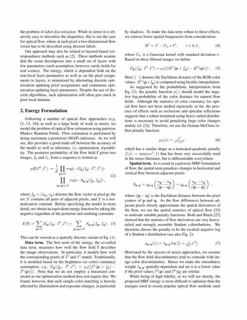
(a) First Frame (b) Ground truth (c) Final Solution, Energy=2041

(d) Solution 1, Energy=7264 (e) Solution 2, Energy=44859 (f) Auxiliary variables (g) Fused solution, Energy=6022

Figure 3. Results for the Army sequence from [1]. The bottom row shows the first step of our discrete optimization (where ”Lucas-Kanade meets Horn-Schunck”). Here, a randomly chosen initial solution (d) (computed with Horn-Schunck) is fused with another ran-domly chosen proposal solution (e) (computed with Lucas-Kanade). The graph cut allows to compute the optimal fused solution (g) withmuch lower energy, which is passed on to the next iteration. The optimal auxiliary variables (f) show which regions are taken from Solution1 (black) and from Solution 2 (white). In this example 99.998% of the nodes were labeled by the minimum cut on the extended graph.

the Horn-Schunck (HS) method [14]. Such solutions oftencontain good results for regions with smooth motion, butmotion discontinuities are always severely oversmoothed.Finally, we also used constant flow fields as proposals.

To obtain a rich set of proposal solutions, we use the LKand HS methods with various parameter settings. For HSwe vary the strength of the regularization (λ ∈ 1, 3, 100).Since both methods should be applied within a coarse-to-fine warping framework to overcome the limitations of thelinearized data term (of the proposals, not of our energy),we also vary the number of levels in the coarse-to-fine hier-archy (l ∈ 1, . . . , 5). Finally, for all LK solutions anda few HS solutions we produce shifted copies (by shift-ing ±2l−1 and ±2l pixels in each direction). For the LKmethod, this corresponds to the use of a family of non-centralized windows and, hence, gives better chances ofproviding correct flow values near flow discontinuities, andas we found reduces the energy of the solution. These varia-tions result in about 200 proposals (most of them, however,are shifted copies and do not take much time to compute).64 constant flow fields are also added to the set of proposals.The choice of the constants is discussed below.

It is important to note that other (potentially more effi-cient) approaches for obtaining proposal solutions may alsobe considered. We also experimented with proposal solu-tions by performing gradient descent from different startingpoints. We found this to lead to good results (given a suffi-cient number of minima), but did not pursue it in our finalexperiments due to its computational inefficiency.

Discrete optimization. As described above, the pro-posal solutions are fused by computing the minimal cut onthe extended graph. The process starts with the LK and HS

proposal fields only. One of these proposal fields is ran-domly chosen as an initial solution. After that, the remain-ing LK and HS proposals are visited in random order, andeach of them is fused with the current solution (as describedin Sec. 3.1). An example of such a fusion (during the firstiteration of the process) is shown in Fig. 3.

After all LK and HS solutions are visited, the motionvectors of the obtained fused solution are clustered into 64clusters using the k-means algorithm. The centers of theclusters ci ∈ R2 are used to produce constant proposal flowfields fi(p) ≡ ci. Note that more sophisticated proposalsdependent on the current solution may be suggested and ourconstant solutions are just one step in this direction.

The created constant proposals are added to the LK andHS proposals and the fusion process continues until eachproposal is visited twice more. At this point the proceduretypically converges, i.e., the obtained fused solution can nolonger be changed by fusion with any of the proposals.

We should note that the number of unlabeled nodes dur-ing each fusion was always negligible (we never observedit exceeding 0.1% of the nodes). Each fusion is guaranteednot to increase the energy, and in practice the resulting so-lution always has an energy that is much smaller than theenergy of the best proposal.

Continuous optimization. After fusing flow fields us-ing discrete optimization, we perform a continuous opti-mization step that helps “cleaning up” areas where the pro-posal solutions were not diverse enough, which for exam-ple may happen in relatively smooth areas. In order to per-form continuous optimization, we analytically compute thegradient of the same energy we use in the discrete step,∇fE(f), and use a standard conjugate gradient method [24]

to perform local optimization. The gradient of the spa-tial term is quite easily derived; computing the gradient ofthe data term relies on the fact that H1(p + fp) is com-puted using bicubic interpolation, which allows computingthe partial derivatives w.r.t. up and vp. We should note thatthe gradient bears resemblance to the discretization of theEuler-Lagrange equations for the objective used in [23].

Since the discrete optimization step avoids many of thepoor local optima that are problematic for purely continu-ous optimization methods, the combination of discrete andcontinuous optimization leads to local minima with a sub-stantially lower energy in most of our experiments.

4. EvaluationTo evaluate the proposed approach and in particular the

efficiency of the proposed energy minimization scheme inobtaining low-energy states of Eq. (3), we performed anumber of experiments using the recent Middlebury opticalflow benchmark dataset [1]. Since our method is applica-ble to color images and based on 2 frames, we used the 2-frame color versions of the datasets, and left the extension tomulti-frame sequences for future work. In all experiments,we used an 8-neighborhood system for the spatial term andthe following parameters, which were chosen to give goodperformance on challenging real-world scenes: σ = 1.5 forthe high-pass filter, µ = 16 and ν = 0.2 for the MRF po-tentials; λp,q = 0.024, if the sum of absolute differencesbetween I(p, t) and I(q, t) was less than or equal to 30,and λp,q = 0.008 otherwise.

We evaluated the proposed method on 8 benchmarkingsequences and found that it outperforms other methods inthe benchmark, particularly on the challenging real worldscenes as they are shown in Fig. 1, Fig. 3 and Fig. 4. Atthe moment of publication, the proposed method was top-ranked on 10 out of 16 available performance measures in-cluding the average angular error (AAE) and the averageend-point error. The only sequence, where our methoddoes not perform well is the Yosemite sequence. This ismainly due to the fact that our parameters were chosen togive good performance on real-world sequences (increas-ing the smoothness weight by 16x without changing otherparameters lowers the AAE on Yosemite from 4.55 to 2.33degrees).

Proposed energy vs. baseline energy. To evaluate theadvantage of the proposed energy, we also considered asimple “baseline” energy that is quite similar to the ob-jectives in popular continuous methods [9, 23]. In partic-ular, we again use an 8-neighborhood for the spatial term,but here with convex Charbonnier potentials (Ch(x, φ) =φ2√

1 + x2/φ2), which are similar to the absolute differ-ence measure (see also Fig. 2). The trade-off weight λ wasnot adapted spatially. For the data term, we used gray-scale images as input from which we did not remove the

low frequencies, and also relied on Charbonnier potentials.We optimized the energy using the approach proposed here,and tuned the parameters of the baseline model using gridsearch on “RubberWhale” (see Fig. 5). As can be seenin Fig. 5a and c, the proposed energy clearly outperformsthe baseline model visually and quantitatively, even on thesequence used to tune the baseline energy parameters. Inparticular, the robust spatial potentials employed here allowto recover sharp discontinuities, while at the same time re-covering smooth flow fields in continuous areas (Fig. 5c).Also, the robust data potentials allowed to attain better per-formance in occlusion areas. Finally, ignoring low fre-quency image content substantially improved the results inareas with shadows, such as on “Schefflera”, from whichthe baseline model suffers.

Our optimization vs. other schemes. For our energy,we also compared the proposed discrete-continuous opti-mization method with a baseline continuous and a baselinediscrete optimization scheme. For baseline continuous op-timization, we employed a hierarchical coarse-to-fine esti-mation framework with 5 levels (c.f . [3]), where at eachpyramid level we used the gradient descent scheme de-scribed in Sec. 3.2. As a baseline discrete algorithm, weran α-expansion (i.e. “conventional” graph cuts) [7]. Tomake the comparison more favorable for this baseline algo-rithm, we estimated the minimum and maximum horizontaland vertical flow from our high-quality solution (note thatsuch an accurate estimate cannot be obtained directly fromproposal solutions), and discretized this range uniformly togive about 1000 labels (i.e., 4 times larger than the numberof proposals that the fusion approach uses).

We found that neither of the two baseline energy mini-mization schemes gave good results for our energy consis-tently across the benchmark datasets, neither in terms of theenergy, nor in terms of flow accuracy (see Tab. 1). In par-ticular, the continuous baseline algorithm failed on most ofthe datasets (see, e.g., Fig. 5b). This suggests that the pro-posed energy is simply too difficult for standard continuousoptimization approaches, for example because of the non-convex potentials and the removal of low frequencies in thedata term. While the behavior of the continuous optimiza-tion could be improved, for example using deterministic an-nealing (c.f . [3]), such heuristics rarely work well across awide-range of datasets. The baseline discrete algorithm ob-viously suffered from the uniformity of discretization, espe-cially for the datasets with large motion (e.g., “Urban”).

How many proposals? In our experiments we focusedon the accuracy of optical flow estimation, thus using ex-tensive numbers of proposals and an exhaustive number ofiterations within continuous optimization. As a result, ourunoptimized MATLAB implementation takes more than anhour for processing a single frame pair.

It is important, nevertheless, to emphasize that flow fu-

Figure 4. Example results on the benchmark datasets (right) along with ground truths (left).

Optimiz.Army

AAE E(f)Mequon

AAE E(f)Schefflera

AAE E(f)Wooden

AAE E(f)Grove

AAE E(f)Urban

AAE E(f)Yosemite

AAE E(f)Teddy

AAE E(f)Our (full) 4.43 2041 2.47 3330 3.70 5778 3.68 1632 4.06 17580 6.30 5514 4.55 1266 7.12 9315

Our (discrete) 4.97 2435 4.83 4375 5.14 7483 5.24 2180 4.00 21289 6.27 6568 4.03 1423 6.68 10450Baseline cont. 7.97 4125 52.3 21417 36.1 24853 16.8 7172 64.0 78122 46.1 26517 23.2 4470 63.9 31289Baseline disc. 5.61 3038 5.19 6209 5.36 8894 4.94 2782 9.03 44450 18.7 17770 5.67 1995 9.13 15283

Table 1. Comparison of different optimization techniques: our full discrete-continuous, our discrete (i.e., fusion of proposals withoutcontinuous improvement), baseline continuous, baseline discrete. Shown are the flow accuracy (average angular error) and the energyachieved. On the 8 test datasets [1], our optimization scheme consistently outperforms the two baseline algorithms.

Energy vs. # of proposals Error vs. # of proposals

Figure 6. The energy and the average angular error (AAE) afterthe discrete optimization step for different subsets of proposals for“Rubber Whale” [1]. The x-coordinate of each dot corresponds tothe number of proposals in the subset. The rightmost point on eachplot corresponds to the full set of proposals. The plots suggest thatsets of proposals that are 5 time smaller would do almost as wellin our experiments.

sion idea is useful in scenarios where speed matters. Fig. 3shows one such example, where fusion of just two motionfields (each computed with real-time methods) improves theresult over both of them. Note that one fusion takes frac-tions of a second. Fig. 6 further explores the trade-off be-tween the number of proposals and the quality of the solu-tion for one of the sequences from [1]. It demonstrates thata five-fold reduction in the number of proposals leads tosolutions that are only slightly worse than those computedwith the full set of proposals.

We also tried to fuse both the discrete and the discrete-continuous results with the known ground truth on “Rub-

ber Whale” to determine the quality of our proposals. Wefound a mild energy reduction in the discrete case (fromE = 1821 to 1756), but hardly any reduction in the discrete-continuous case (from E = 1613 to 1610). This showsthat our proposals appear to be very appropriate, as evenknowing the ground truth will not lower the energy much,and that the continuous improvement step substantially im-proves the results toward the ground truth (especially insmoothly varying areas). Furthermore, this also suggeststhat the proposed optimization gets very close to the groundtruth (as much as is permitted by the model) and that furtheraccuracy gains will require more involved models.

5. Conclusions

In this paper we proposed a new energy minimizationapproach for optical flow estimation called FusionFlow thatcombines the advantages of discrete and continuous opti-mization. The power of the optimization method allowedus to leverage a complex, highly non-convex energy for-mulation, which is very challenging for traditional contin-uous optimization methods. The proposed energy formu-lation was motivated by the statistics of optical flow, bor-rows from the stereo literature, and is robust to brightnesschanges, such as in shadow regions. Experimentally, at themoment of publication our approach is the top-performingmethod on the Middlebury optical flow benchmark across avariety of complex real-world scenes.

(a) Baseline energy, discrete-continuous optimization. (Left) RubberWhale: AAE=5.169. (Right) Schefflera

(b) Our energy, baseline continuous optimization. (Left) RubberWhale: E=4149, AAE=6.72. (Right) Schefflera: E=24853

(c) Our energy, discrete-continuous optimization. (Left) RubberWhale: E=1861, AAE=3.68. (Right) Schefflera: E=5778

Figure 5. Results for different energies and optimization methods. Each part shows the estimated flow field as well as a detail of the result.

Future work should consider whether more efficient pro-posal solutions can be developed that offer a similar diver-sity, but using many fewer proposals to reduce run-time.With very few proposals, very fast flow estimation mighteven be possible, at least without continuous refinement.

References[1] S. Baker, D. Scharstein, J. Lewis, S. Roth, M. J. Black, and

R. Szeliski. A database and evaluation methodology for optical flow.ICCV 2007 http://vision.middlebury.edu/flow/ .

[2] S. Birchfield, B. Natarjan, and C. Tomasi. Correspondence as energy-based segmentation. Image Vision Comp., 25(8):1329–1340, 2007.

[3] M. J. Black and P. Anandan. The robust estimation of multiple mo-tions: Parametric and piecewise-smooth flow fields. CVIU, 63(1):75–104, 1996.

[4] E. Boros, P. Hammer, and G. Tavares. Preprocessing of uncon-strained quadratic binary optimization. Technical Report RUTCORRRR 10-2006.

[5] E. Boros and P.L.Hammer. Pseudo-boolean optimization. DiscreteApplied Mathematics, 123(1-3):155–225, 2002.

[6] Y. Boykov and V. Kolmogorov. An experimental comparison of min-cut/max-flow algorithms for energy minimization in vision. TPAMI,26(9):1124–1137, 2004.

[7] Y. Boykov, O. Veksler, and R. Zabih. Fast approximate energy mini-mization via graph cuts. TPAMI, 23(11):1222–1239, 2001.

[8] T. Brox, A. Bruhn, and J. Weickert. Variational motion segmentationwith level sets. ECCV 2006, v. 1, pp. 471–483.

[9] A. Bruhn, J. Weickert, and C. Schnorr. Lucas/Kanade meetsHorn/Schunck: Combining local and global optic flow methods.IJCV, 61(3):211–231, 2005.

[10] P. F. Felzenszwalb and D. P. Huttenlocher. Efficient belief propaga-tion for early vision. CVPR 2004, v. 1, pp. 261–268.

[11] B. Glocker, N. Komodakis, N. Paragios, G. Tziritas, and N. Navab.Inter and intra-modal deformable registration: Continuous deforma-tions meet efficient optimal linear programming. IPMI 2007.

[12] D. Greig, B. Porteous, and A. Seheult. Exact MAP estimation forbinary images. J. Roy. Stat. Soc. B, 51(2):271–279, 1989.

[13] F. Heitz and P. Bouthemy. Multimodal estimation of discontinu-ous optical flow using Markov random fields. TPAMI, 15(12):1217–1232, 1993.

[14] B. K. P. Horn and B. G. Schunck. Determining optical flow. ArtificialIntelligence, 17(1–3):185–203, 1981.

[15] H. Ishikawa. Exact optimization for Markov random fields with con-vex priors. TPAMI, 25(10):1333–1336, 2003.

[16] V. Kolmogorov and C. Rother. Minimizing non-submodular func-tions with graph cuts — A review. TPAMI, 29(7):1274–1279, 2006.

[17] V. Kolmogorov and R. Zabih. What energy functions can be mini-mized via graph cuts? TPAMI, 24(2):147–159, 2004.

[18] J. Konrad and E. Dubois. Multigrid Bayesian estimation of imagemotion fields using stochastic relaxation. ICCV 1988, pp. 354–362.

[19] V. Lempitsky, C. Rother, and A. Blake. LogCut - Efficient graph cutoptimization for Markov random fields. ICCV 2007.

[20] B. D. Lucas and T. Kanade. An iterative image registration techniquewith an application to stereo vision. IJCAI, pp. 674–679, 1981.

[21] T. Meltzer, C. Yanover, and Y. Weiss. Globally optimal solutions forenergy minimization in stereo vision using reweighted belief propa-gation. ICCV 2005, v. 1, pp. 428–435.

[22] E. Memin and P. Perez. Hierarchical estimation and segmentation ofdense motion fields. IJCV, 46(2):129–155, 2002.

[23] N. Papenberg, A. Bruhn, T. Brox, S. Didas, and J. Weickert. Highlyaccurate optic flow computation with theoretically justified warping.IJCV, 67(2):141–158, 2006.

[24] C. E. Rasmussen. minimize.m. http://www.kyb.tuebingen.

mpg.de/bs/people/carl/code/minimize/ , 2006.[25] S. Roth and M. J. Black. On the spatial statistics of optical flow.

IJCV, 74(1):33–50, 2007.[26] C. Rother, V. Kolmogorov, V. Lempitsky, and M. Szummer. Opti-

mizing binary MRFs via extended roof duality. CVPR 2007.[27] A. Shekhovtsov, I. Kovtun, and V. Hlavac. Efficient MRF deforma-

tion model for non-rigid image matching. CVPR 2007.[28] J. Sun, N.-N. Zhen, and H.-Y. Shum. Stereo matching using belief

propagation. TPAMI, 25(7):787–800, 2003.