Embed Size (px)
Citation preview
x
Trains travelling at speeds in excess of 200 kmh � 1 have greatly reduced the journey time to continental cities. Mechanical principles are applied in the calculation of the tractive eff ort required to maintain these speeds and the braking forces required to bring the trains to rest. Mechanical principles are also applied in the design of tilting mechanisms and the track infrastructure.
Photo courtesy of iStockphoto, Remus Eserblom, Image# 4619117
CH001.indd xCH001.indd x 4/22/2010 10:01:23 PM4/22/2010 10:01:23 PM
Further Mechanical Principles and Applications
T he design, manufacture and servicing of engineered products are important to the nation ’ s economy and well-being. One has only to think of the information technology (IT) hardware, aircraft, motor vehicles and domestic appliances
we use in everyday life to realise how reliant we have become on engineered products. A product must be fi t for its purpose. It must do the job for which it was designed for a reasonable length of time and with a minimum of maintenance. The term ‘ mechatronics ’ is often used to describe products which contain mechanical, electrical, electronic and IT systems. It is the aim of this chapter to broaden your knowledge of the underpinning mechanical principles which are fundamental to engineering design, manufacturing and servicing.
Chapter 1
1
CH001.indd 1CH001.indd 1 4/22/2010 10:01:29 PM4/22/2010 10:01:29 PM
Further Mechanical Principles and Applications
CHAP
TER
12
Engineering Structures
Loading systems
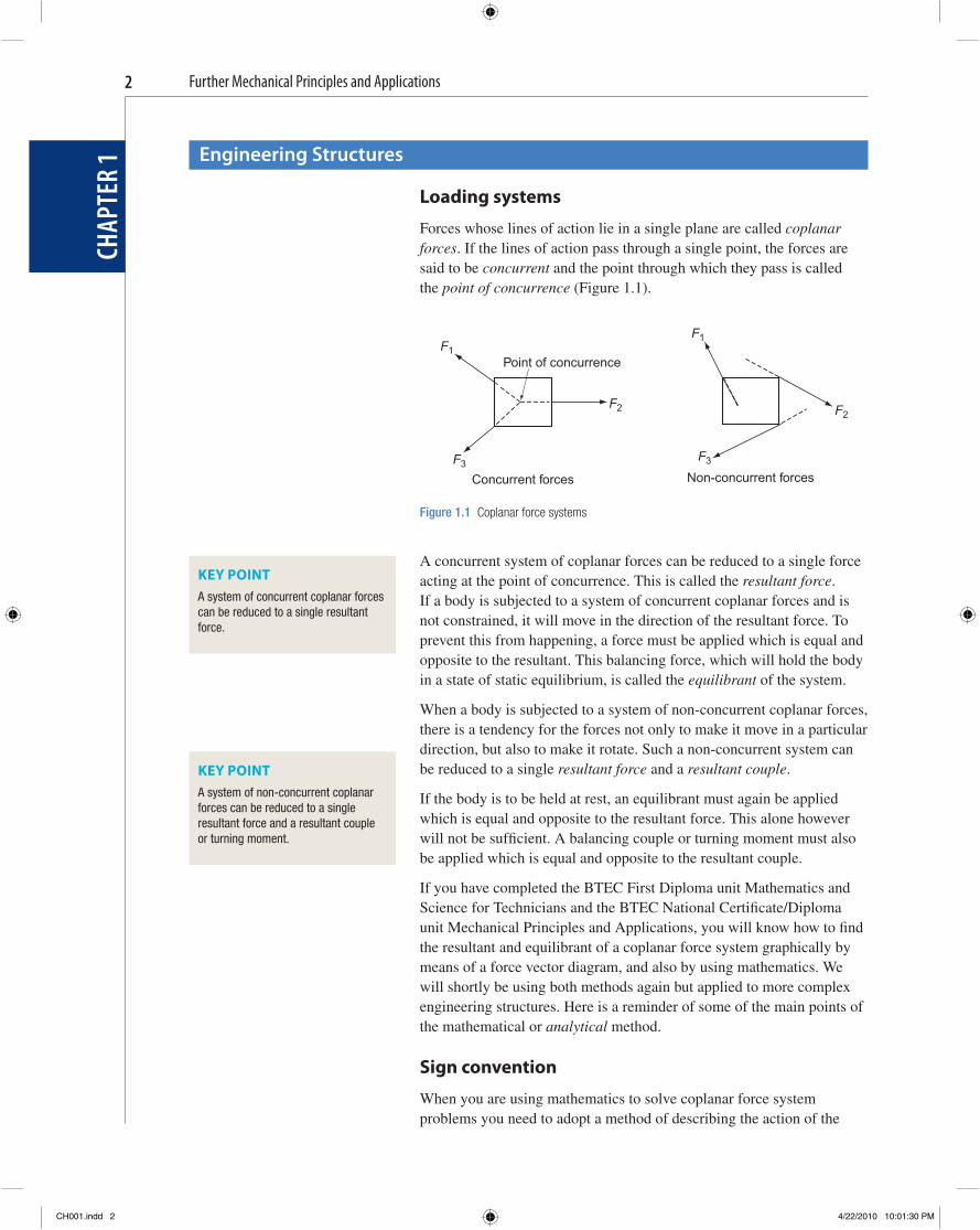
Forces whose lines of action lie in a single plane are called coplanar forces . If the lines of action pass through a single point, the forces are said to be concurrent and the point through which they pass is called the point of concurrence ( Figure 1.1 ).
F1
F2F2
F3
F1
F3
Point of concurrence
Concurrent forces Non-concurrent forces
Figure 1.1 Coplanar force systems
A concurrent system of coplanar forces can be reduced to a single force acting at the point of concurrence. This is called the resultant force . If a body is subjected to a system of concurrent coplanar forces and is not constrained, it will move in the direction of the resultant force. To prevent this from happening, a force must be applied which is equal and opposite to the resultant. This balancing force, which will hold the body in a state of static equilibrium, is called the equilibrant of the system.
When a body is subjected to a system of non-concurrent coplanar forces, there is a tendency for the forces not only to make it move in a particular direction, but also to make it rotate. Such a non-concurrent system can be reduced to a single resultant force and a resultant couple .
If the body is to be held at rest, an equilibrant must again be applied which is equal and opposite to the resultant force. This alone however will not be suffi cient. A balancing couple or turning moment must also be applied which is equal and opposite to the resultant couple.
If you have completed the BTEC First Diploma unit Mathematics and Science for Technicians and the BTEC National Certifi cate/Diploma unit Mechanical Principles and Applications, you will know how to fi nd the resultant and equilibrant of a coplanar force system graphically by means of a force vector diagram, and also by using mathematics. We will shortly be using both methods again but applied to more complex engineering structures. Here is a reminder of some of the main points of the mathematical or analytical method.
Sign convention
When you are using mathematics to solve coplanar force system problems you need to adopt a method of describing the action of the
KEY POINT A system of concurrent coplanar forces can be reduced to a single resultant force.
KEY POINT A system of non-concurrent coplanar forces can be reduced to a single resultant force and a resultant couple or turning moment.
CH001.indd 2CH001.indd 2 4/22/2010 10:01:30 PM4/22/2010 10:01:30 PM

Further Mechanical Principles and Applications
CHAP
TER
1
3
forces and couples. The following sign convention is that which is most often used:
(i) Upward forces are positive and downward forces are negative. (ii) Horizontal forces acting to the right are positive and horizontal
forces acting to the left are negative. (iii) Clockwise acting moments and couples are positive and
anticlockwise acting moments and couples are negative.
+
+−
−
M M+ −
Figure 1.2 Sign convention
F
(a)
FH
FH
FV FV
(b)
F
θ
θ
Figure 1.3 Resolution of forces
Resolution of forces
Forces which act at an angle exert a pull which is part horizontal and part vertical. They can be split into their horizontal and vertical parts or components , by the use of trigonometry. When you are doing this, it is a useful rule to always measure angles to the horizontal ( Figure 1.3 ).
In Figure 1.3(a) the horizontal and vertical components are both acting in the positive directions and will be:
F F F FH vcos sin� � � �� �and
In Figure 1.3(b) the horizontal and vertical components are both acting in the negative directions and will be:
F F F FH vcos sin� � � �� �and
Forces which act upwards to the left or downwards to the right will have one component which is positive and one which is negative. Having resolved all of the forces in a coplanar system into their horizontal and vertical components, each set can then be added algebraically to determine the resultant horizontal pull, � F H , and the resultant vertical
CH001.indd 3CH001.indd 3 4/22/2010 10:01:31 PM4/22/2010 10:01:31 PM
Further Mechanical Principles and Applications
CHAP
TER
14
pull, � F V . The Greek letter � (sigma) means ‘ the sum or total ’ of the components. Pythagoras ’ theorem can then be used to fi nd the single resultant force R of the system.
i.e. 2 2R F F2H V ( ) ( )� �� �
R F F� ( ) ( )H V� �2 2�
(1.1)
The angle � which the resultant makes with the horizontal can also be found using:
tan V
H
� ��F
F� (1.2)
With non-concurrent force systems, the algebraic sum of the moments of the vertical and horizontal components of the forces, taken about some convenient point, gives the resultant couple or turning moment. Its sign, positive or negative, indicates whether its direction is clockwise or anticlockwise. This in turn can be used to fi nd the perpendicular distance of the line of action of the resultant from the chosen point.
Example 1.1
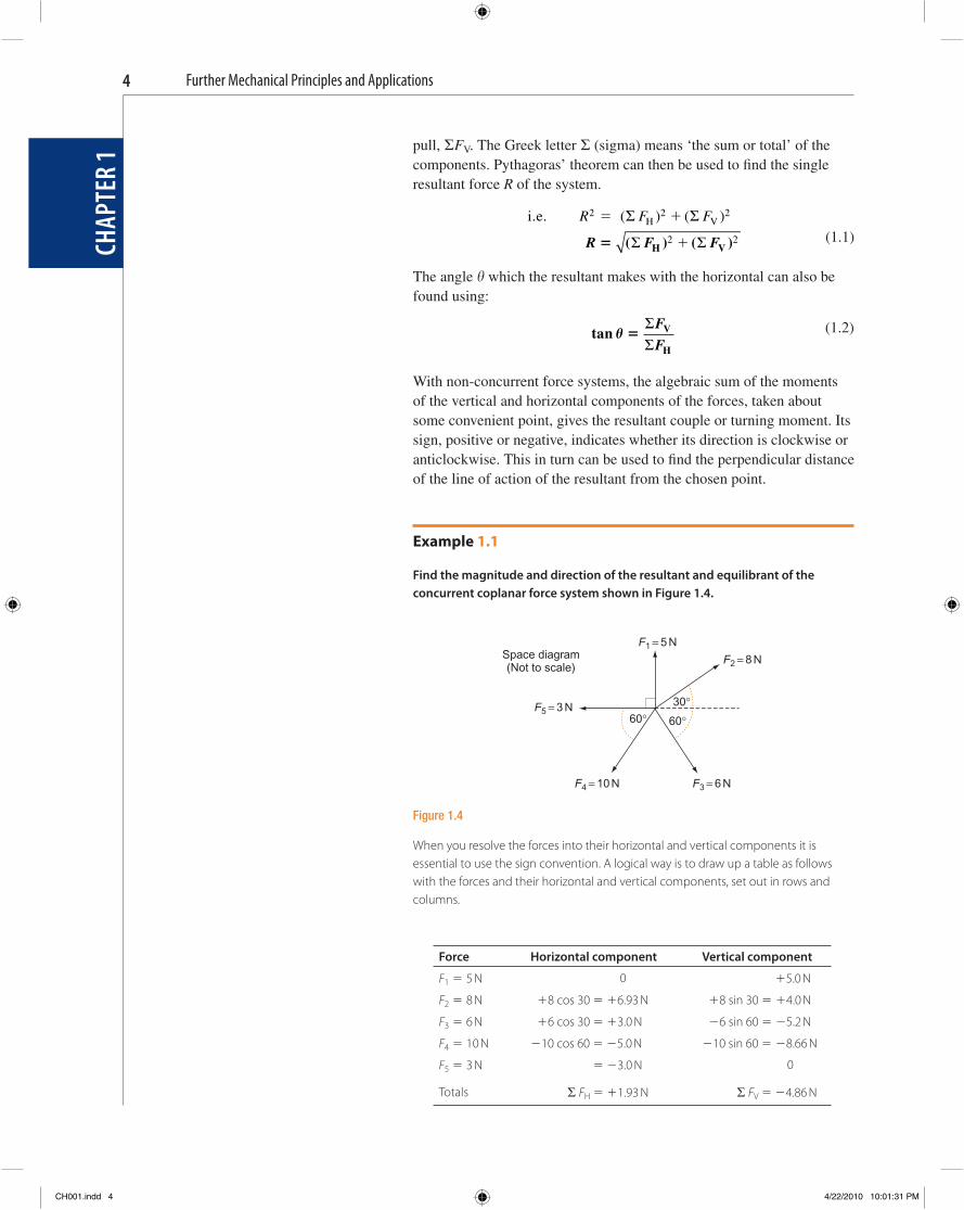
Find the magnitude and direction of the resultant and equilibrant of the concurrent coplanar force system shown in Figure 1.4 .
Space diagram(Not to scale)
F5 = 3 N
F4 = 10 N F3 = 6 N
F2 = 8 N
F1 = 5 N
60° 60°
30°
Figure 1.4
When you resolve the forces into their horizontal and vertical components it is essential to use the sign convention. A logical way is to draw up a table as follows with the forces and their horizontal and vertical components, set out in rows and columns.
Force Horizontal component Vertical component
F1 � 5 N 0 �5.0 N
F2 � 8 N �8 cos 30 � �6.93 N �8 sin 30 � �4.0 N
F3 � 6 N �6 cos 30 � �3.0 N �6 sin 60 � �5.2 N
F4 � 10 N �10 cos 60 � �5.0 N �10 sin 60 � �8.66 N
F5 � 3 N � �3.0 N 0
Totals � FH � �1.93 N � FV � �4.86 N
CH001.indd 4CH001.indd 4 4/22/2010 10:01:31 PM4/22/2010 10:01:31 PM
Further Mechanical Principles and Applications
CHAP
TER
1
5
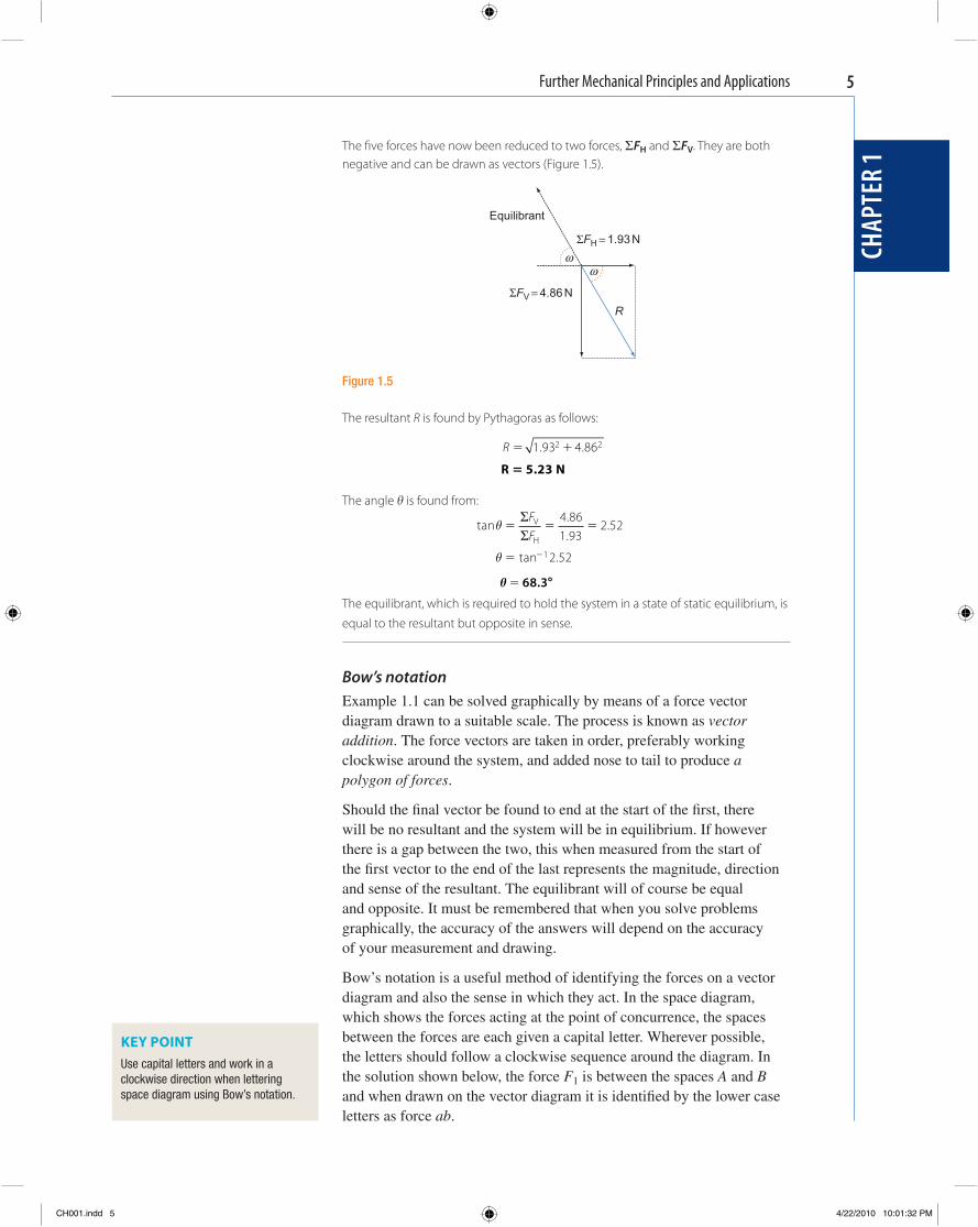
The fi ve forces have now been reduced to two forces, � F H and � F V . They are both negative and can be drawn as vectors ( Figure 1.5 ).
Equilibrant
R
ΣFH = 1.93 N
ΣFV = 4.86 N
ωω
Figure 1.5
The resultant R is found by Pythagoras as follows:
R � �1 93 4 862 2. . R 5.23 N�
The angle � is found from:
tan
tan
V
H
θ
θ
� � �
� �
��
FF
4 861 93
2 52
2 521
.
..
.
� � 68 3. � The equilibrant, which is required to hold the system in a state of static equilibrium, is
equal to the resultant but opposite in sense.
Bow ’ s notation Example 1.1 can be solved graphically by means of a force vector diagram drawn to a suitable scale. The process is known as vector addition . The force vectors are taken in order, preferably working clockwise around the system, and added nose to tail to produce a polygon of forces .
Should the fi nal vector be found to end at the start of the fi rst, there will be no resultant and the system will be in equilibrium. If however there is a gap between the two, this when measured from the start of the fi rst vector to the end of the last represents the magnitude, direction and sense of the resultant. The equilibrant will of course be equal and opposite. It must be remembered that when you solve problems graphically, the accuracy of the answers will depend on the accuracy of your measurement and drawing.
Bow ’ s notation is a useful method of identifying the forces on a vector diagram and also the sense in which they act. In the space diagram, which shows the forces acting at the point of concurrence, the spaces between the forces are each given a capital letter. Wherever possible, the letters should follow a clockwise sequence around the diagram. In the solution shown below, the force F 1 is between the spaces A and B and when drawn on the vector diagram it is identifi ed by the lower case letters as force ab .
KEY POINT Use capital letters and work in a clockwise direction when lettering space diagram using Bow ’ s notation.
CH001.indd 5CH001.indd 5 4/22/2010 10:01:32 PM4/22/2010 10:01:32 PM
Further Mechanical Principles and Applications
CHAP
TER
16
The clockwise sequence of letters on the space diagram, i.e. A to B, gives the direction of the force on the vector diagram. The letter a is at the start of the vector and the letter b is at its end. Although arrows have been drawn to show the directions of the vectors they are not really necessary and will be omitted on future graphical solutions.
Example 1.2
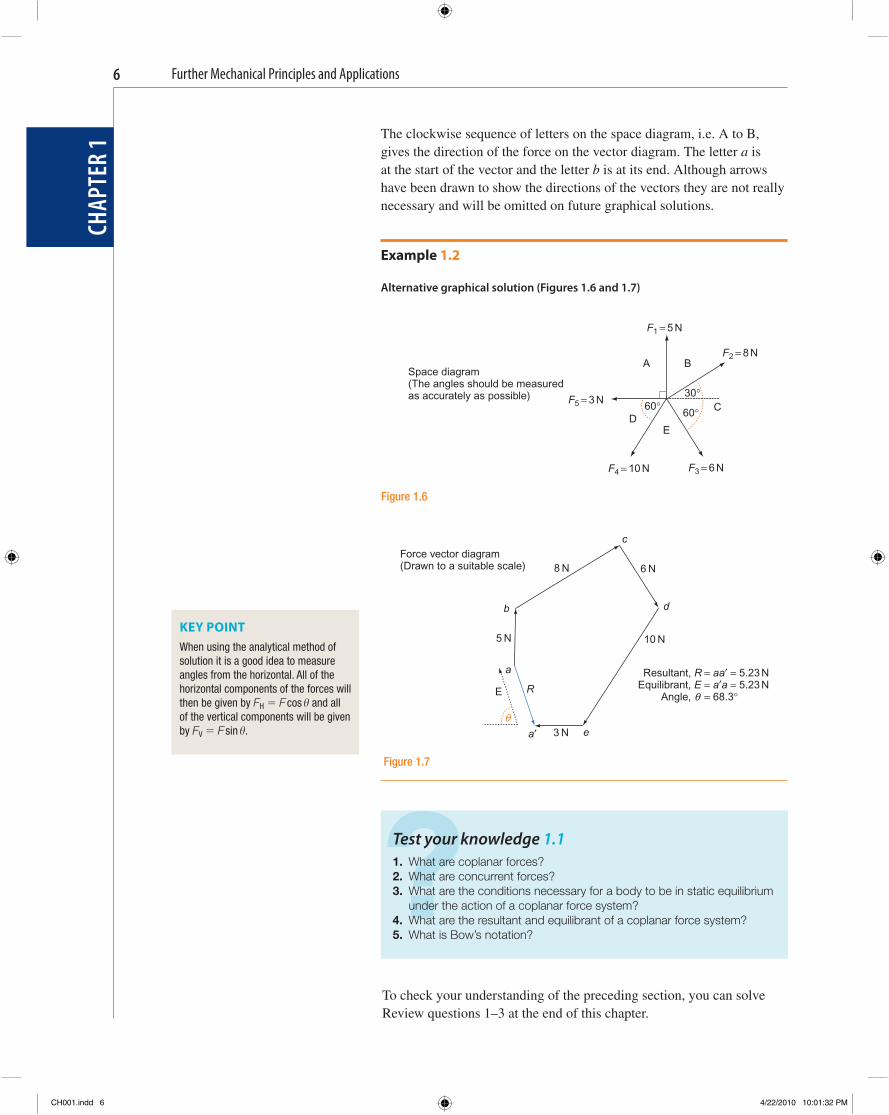
Alternative graphical solution ( Figures 1.6 and 1.7 )
F1 = 5 N
F5 = 3 N
F4 = 10 N F3 = 6 N
F2 = 8 N
Space diagram(The angles should be measuredas accurately as possible)
60°60°
30°C
DE
A B
Figure 1.6
KEY POINT When using the analytical method of solution it is a good idea to measure angles from the horizontal. All of the horizontal components of the forces will then be given by F H � F cos � and all of the vertical components will be givenby F V � F sin � .
? Test your knowledge 1.1 1. What are coplanar forces? 2. What are concurrent forces? 3. What are the conditions necessary for a body to be in static equilibrium
under the action of a coplanar force system? 4. What are the resultant and equilibrant of a coplanar force system? 5. What is Bow ’ s notation?
To check your understanding of the preceding section, you can solve Review questions 1–3 at the end of this chapter.
Force vector diagram(Drawn to a suitable scale)
c
db
10 N 5 N
a Resultant, R = aa′ = 5.23 NEquilibrant, E = a′a = 5.23 N Angle, = 68.3° E R
a′ e3 N
6 N8 N
θ
θ
Figure 1.7
CH001.indd 6CH001.indd 6 4/22/2010 10:01:32 PM4/22/2010 10:01:32 PM
Further Mechanical Principles and Applications
CHAP
TER
1
7
Pin-jointed framed structures
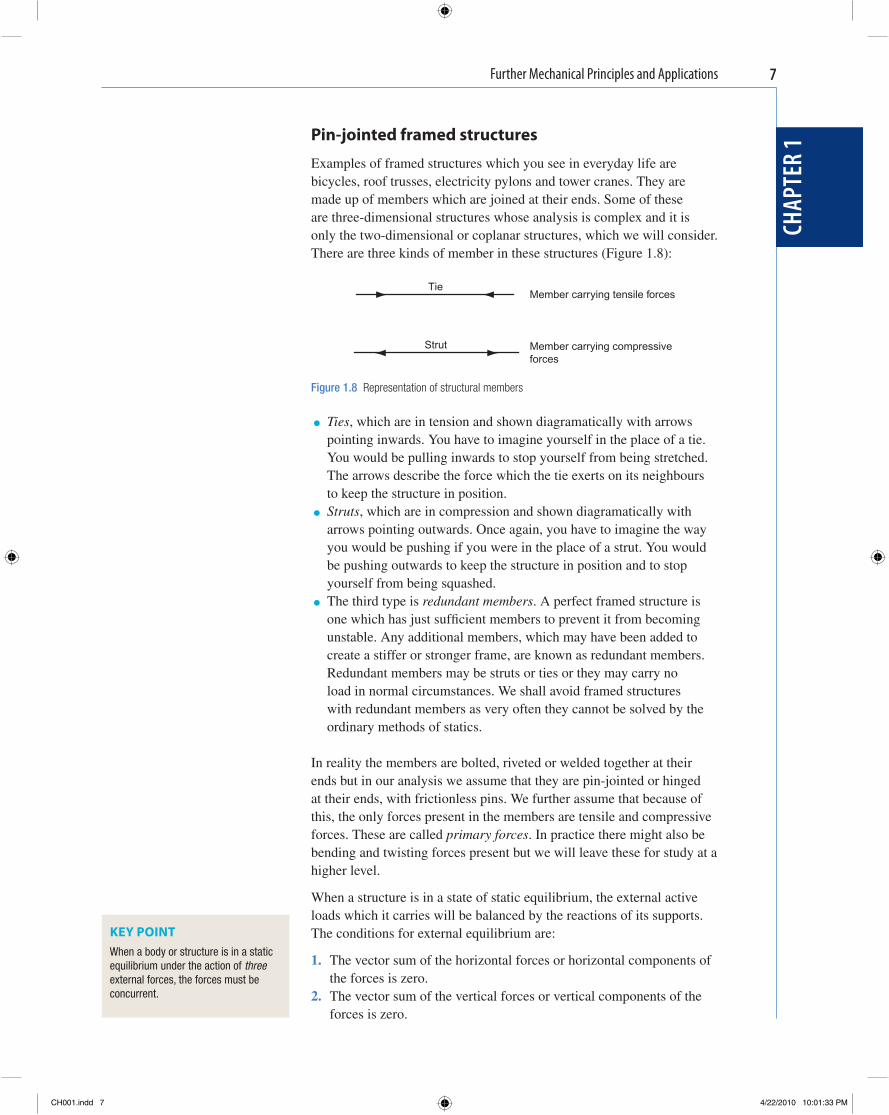
Examples of framed structures which you see in everyday life are bicycles, roof trusses, electricity pylons and tower cranes. They are made up of members which are joined at their ends. Some of these are three-dimensional structures whose analysis is complex and it is only the two-dimensional or coplanar structures, which we will consider. There are three kinds of member in these structures ( Figure 1.8 ):
TieMember carrying tensile forces
Strut Member carrying compressiveforces
Figure 1.8 Representation of structural members
● Ties , which are in tension and shown diagramatically with arrows pointing inwards. You have to imagine yourself in the place of a tie. You would be pulling inwards to stop yourself from being stretched. The arrows describe the force which the tie exerts on its neighbours to keep the structure in position.
● Struts , which are in compression and shown diagramatically with arrows pointing outwards. Once again, you have to imagine the way you would be pushing if you were in the place of a strut. You would be pushing outwards to keep the structure in position and to stop yourself from being squashed.
● The third type is redundant members . A perfect framed structure is one which has just suffi cient members to prevent it from becoming unstable. Any additional members, which may have been added to create a stiffer or stronger frame, are known as redundant members. Redundant members may be struts or ties or they may carry no load in normal circumstances. We shall avoid framed structures with redundant members as very often they cannot be solved by the ordinary methods of statics.
In reality the members are bolted, riveted or welded together at their ends but in our analysis we assume that they are pin-jointed or hinged at their ends, with frictionless pins. We further assume that because of this, the only forces present in the members are tensile and compressive forces. These are called primary forces . In practice there might also be bending and twisting forces present but we will leave these for study at a higher level.
When a structure is in a state of static equilibrium, the external active loads which it carries will be balanced by the reactions of its supports. The conditions for external equilibrium are:
1. The vector sum of the horizontal forces or horizontal components of the forces is zero.
2. The vector sum of the vertical forces or vertical components of the forces is zero.
KEY POINT When a body or structure is in a static equilibrium under the action of three external forces, the forces must be concurrent.
CH001.indd 7CH001.indd 7 4/22/2010 10:01:33 PM4/22/2010 10:01:33 PM
Further Mechanical Principles and Applications
CHAP
TER
18
3. The vector sum of the turning moments of the forces taken about any point in the plane of the structure is zero.
i.e. H V� � �F F M� � �0 0 0
We can also safely assume that if a structure is in a state of static equilibrium, each of its members will also be in equilibrium. It follows that the above three conditions can also be applied to individual members, groups of members and indeed to any internal part or section of a structure.
A full analysis of the external and internal forces acting on and within a structure can be carried out using mathematics or graphically by drawing a force vector diagram. We will use the mathematical method fi rst and begin by applying the conditions for equilibrium to the external forces. This will enable us to fi nd the magnitude and direction of the support reactions.
Next, we will apply the conditions for equilibrium to each joint in the structure, starting with one which has only two unknown forces acting on it. This will enable us to fi nd the magnitude and direction of the force in each member.
Example 1.3
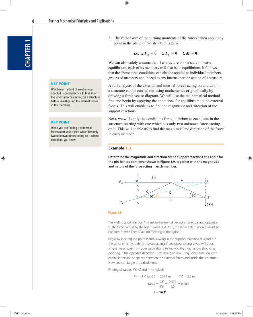
Determine the magnitude and direction of the support reactions at X and Y for the pin-jointed cantilever shown in Figure 1.9 , together with the magnitude and nature of the force acting in each member.
1 mA
Z
RXX P
C D 30° θ 30°
RYB
5 kN
Y
Figure 1.9
KEY POINT Whichever method of solution you adopt, it is good practice to fi nd all of the external forces acting on a structure before investigating the internal forces in the members.
KEY POINT When you are fi nding the internal forces start with a joint which has only two unknown forces acting on it whose directions you know.
The wall support reaction R X must be horizontal because it is equal and opposite to the force carried by the top member CA. Also, the three external forces must be concurrent with lines of action meeting at the point P.
Begin by locating the point P and drawing in the support reactions at X and Y in the sense which you think they are acting. If you guess wrongly, you will obtain a negative answer from your calculations, telling you that your arrow should be pointing in the opposite direction. Letter the diagram using Bow ’ s notation, with capital letters in the spaces between the external forces and inside the structure. Now you can begin the calculations.
Finding distances XY , YZ and the angle � :
XY YZ� � � �1 30 2 0tan 0.577 m m.
tan � � � �
XYYZ
0 5772 0
0 289.
..
� � �16 1.
CH001.indd 8CH001.indd 8 4/22/2010 10:01:33 PM4/22/2010 10:01:33 PM

Further Mechanical Principles and Applications
CHAP
TER
1
9
Take moments about Y to fi nd R X . For equilibrium, � M Y � 0:
( ) .
.
5 2 0 577 0
10 0 577 0
� � � �
� �
( )R
RX
x
RX � �
100 577
17 3.
. kN
The force in member AC will also be 17.3 kN because it is equal and opposite to R X . It will be a tensile force, and this member will be a tie.
Take vertical components of external forces to fi nd R Y . For equilibrium, � F V � 0:
R s
R
y
Y
in16 1 5 0
0 277 5 0
.
.
ο � �
� �
RY � �
50 277
18 0.
. kN
You can now turn your attention to the forces in the individual members. You already know the force F AC acting in member AC because it is equal and opposite to the support reaction R X . Choose a joint where you know the magnitude and direction of one of the forces and the directions of the other two, i.e. where there are only two unknown forces. Joint ABD will be ideal. It is good practice to assume that the unknown forces are tensile, with arrows pulling away from the joint. A negative answer will tell you that the force is compressive ( Figure 1.10 ).
FDA
D A
FBD30°
B
5 kN
Figure 1.10
Take vertical components of the forces to fi nd the force F DA in member DA.
For equilibrium,
sinDA
DA
� F
F
F
v �
� �
� �
0
30 5 0
0 5 5 0.
FDA kN� �
50 5
10.
The positive answer denotes that the force F DA in member DA is tensile and that the member is a tie. Now take horizontal components of the forces to fi nd F BD in member BD.
For equilibrium,
cos
cos
H
DA BD
BD
� F
F F
F
�
� � �
� � �
0
30 0
10 30 0
FBD cos kN�� ��10 30 8 66.
The negative sign denotes that the force F BD in member BD is compressive and that the member is a strut. Now go to joint ADC and take vertical components of the forces to fi nd F DC , the force in member DC ( Figure 1.11 ).
CH001.indd 9CH001.indd 9 4/22/2010 10:01:34 PM4/22/2010 10:01:34 PM
Further Mechanical Principles and Applications
CHAP
TER
110
For equilibrium,
(10 sin ) ( sin )V
DC
DC
� F
F
F
�
� � �
� � �
0
30 30 0
10 0
FDC kN��10
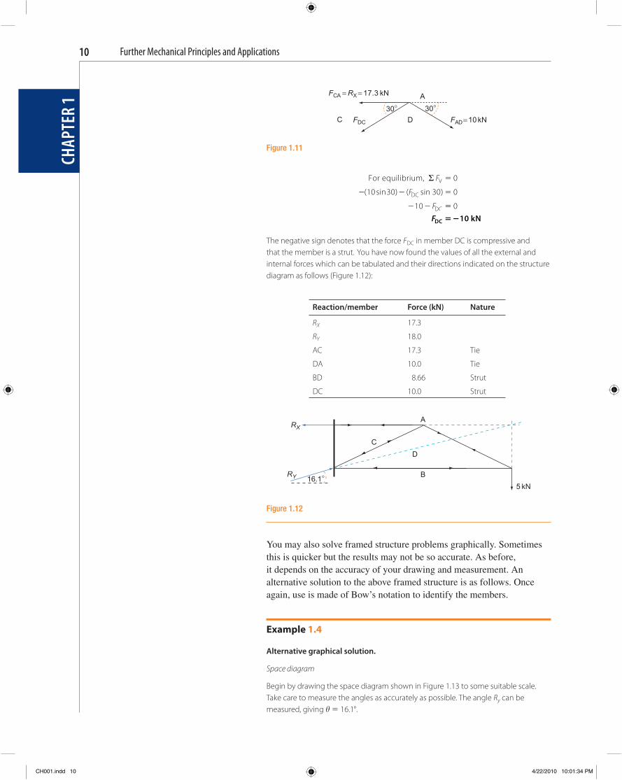
The negative sign denotes that the force F DC in member DC is compressive and that the member is a strut. You have now found the values of all the external and internal forces which can be tabulated and their directions indicated on the structure diagram as follows ( Figure 1.12 ):
FCA = RX = 17.3 kN A
30° 30°C FDC D FAD = 10 kN
Figure 1.11
Reaction/member Force (kN) Nature
RX 17.3
RY 18.0
AC 17.3 Tie
DA 10.0 Tie
BD 8.66 Strut
DC 10.0 Strut
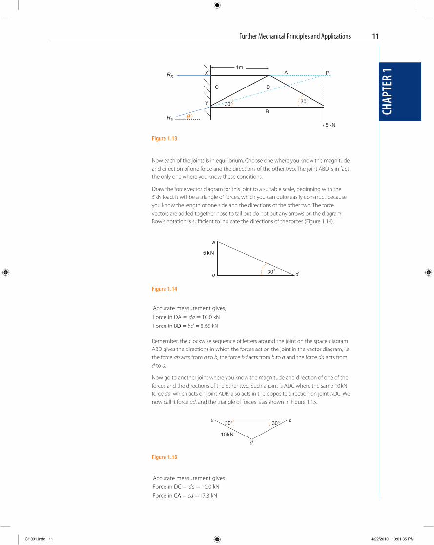
You may also solve framed structure problems graphically. Sometimes this is quicker but the results may not be so accurate. As before, it depends on the accuracy of your drawing and measurement. An alternative solution to the above framed structure is as follows. Once again, use is made of Bow ’ s notation to identify the members.
Example 1.4
Alternative graphical solution.
Space diagram
Begin by drawing the space diagram shown in Figure 1.13 to some suitable scale. Take care to measure the angles as accurately as possible. The angle R y can be measured, giving � � 16.1°.
ARX
C
D
RY B16.1°
5 kN
Figure 1.12
CH001.indd 10CH001.indd 10 4/22/2010 10:01:34 PM4/22/2010 10:01:34 PM
Further Mechanical Principles and Applications
CHAP
TER
1
11
Now each of the joints is in equilibrium. Choose one where you know the magnitude and direction of one force and the directions of the other two. The joint ABD is in fact the only one where you know these conditions.
Draw the force vector diagram for this joint to a suitable scale, beginning with the 5 kN load. It will be a triangle of forces, which you can quite easily construct because you know the length of one side and the directions of the other two. The force vectors are added together nose to tail but do not put any arrows on the diagram. Bow ’ s notation is suffi cient to indicate the directions of the forces ( Figure 1.14 ).
1mARX
X P
C D
Y 30° 30°
RYθ
B
5 kN
Figure 1.13
a
5 kN
b 30° d
Figure 1.14
Accurate measurement gives,
Force in DA kN
Force in B
� �da 10 0.
DD kN� � bd 8 66.
Remember, the clockwise sequence of letters around the joint on the space diagram ABD gives the directions in which the forces act on the joint in the vector diagram, i.e. the force ab acts from a to b , the force bd acts from b to d and the force da acts from d to a .
Now go to another joint where you know the magnitude and direction of one of the forces and the directions of the other two. Such a joint is ADC where the same 10 kN force da , which acts on joint ADB, also acts in the opposite direction on joint ADC. We now call it force ad , and the triangle of forces is as shown in Figure 1.15 .
a c30° 30°
10 kN
d
Figure 1.15
Accurate measurement gives,
Force in DC kN
Force in C
� �dc 10 0.
AA kN� � ca 17 3.
CH001.indd 11CH001.indd 11 4/22/2010 10:01:35 PM4/22/2010 10:01:35 PM

Further Mechanical Principles and Applications
CHAP
TER
112
All of the internal forces have now been found and also the reaction R X , which is equal and opposite to ca , and can thus be written as ac . A fi nal triangle of forces ABC , can now be drawn, representing the three external forces (see Figure 1.16 ). Two of these, th e 5 kN load and R X , are now known in both magnitude and direction together with the angle � which R Y makes with the horizontal.
a cθ
b
Figure 1.16
a c
b d
Figure 1.17
ARx
C
Ry16.1° B
5 kN
D
Figure 1.18
Accurate measurement gives,
Reaction kN
Angle
R bcY � �
�
18 0.
� 116 1. ο
You will note that the above three vector diagram triangles have sides in common and to save time it is usual to draw the second and third diagrams as additions to the fi rst. The combined vector diagram appears as in Figure 1.17 .
The directions of the forces, acting towards or away from the joints on which they act, can be drawn on the space diagram. This will immediately tell you which members are struts and which are ties. The measured values of the support reactions and the forces in the members can then be tabulated ( Figure 1.18 ).
Reaction/member Force (kN) Nature
RX 17.3
RY 18.0
AC 17.3 Tie
DA 10.0 Tie
BD 8.66 Strut
DC 10.0 Strut
CH001.indd 12CH001.indd 12 4/22/2010 10:01:36 PM4/22/2010 10:01:36 PM
Further Mechanical Principles and Applications
CHAP
TER
1
13
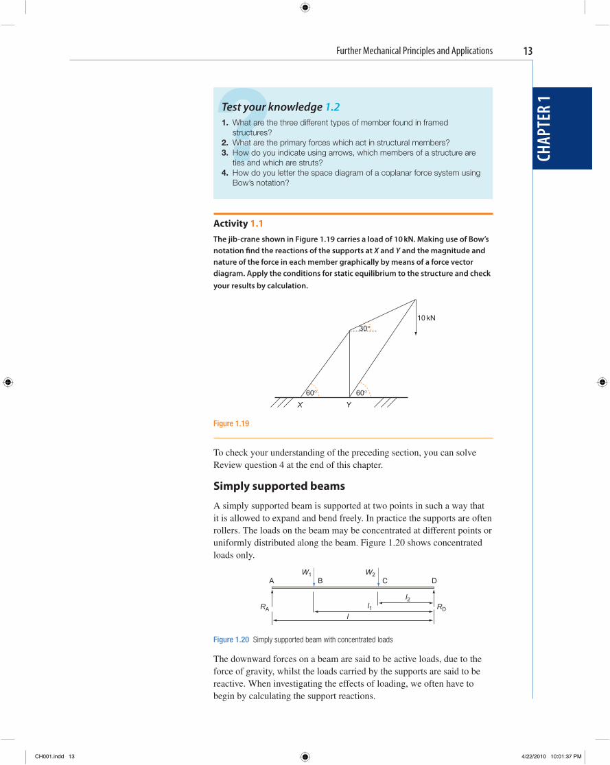
Activity 1.1 The jib-crane shown in Figure 1.19 carries a load of 10 kN. Making use of Bow ’ s notation fi nd the reactions of the supports at X and Y and the magnitude and nature of the force in each member graphically by means of a force vector diagram. Apply the conditions for static equilibrium to the structure and check your results by calculation.
W1 W2A B C D
l2RA l1 RD
l
Figure 1.20 Simply supported beam with concentrated loads
? Test your knowledge 1.2 1. What are the three different types of member found in framed
structures? 2. What are the primary forces which act in structural members? 3. How do you indicate using arrows, which members of a structure are
ties and which are struts? 4. How do you letter the space diagram of a coplanar force system using
Bow ’ s notation?
To check your understanding of the preceding section, you can solve Review question 4 at the end of this chapter.
Simply supported beams
A simply supported beam is supported at two points in such a way that it is allowed to expand and bend freely. In practice the supports are often rollers. The loads on the beam may be concentrated at different points or uniformly distributed along the beam. Figure 1.20 shows concentrated loads only.
The downward forces on a beam are said to be active loads, due to the force of gravity, whilst the loads carried by the supports are said to be reactive. When investigating the effects of loading, we often have to begin by calculating the support reactions.
10 kN
60°
30°
60°X Y
Figure 1.19
CH001.indd 13CH001.indd 13 4/22/2010 10:01:37 PM4/22/2010 10:01:37 PM
Further Mechanical Principles and Applications
CHAP
TER
114
The beam is in static equilibrium under the action of these external forces, and so we proceed as follows.
1. Equate the sum of the turning moments, taken about the right-hand support D, to zero.
i.e. D�M � 0
R l W l W lA � � �1 1 2 2 0
You can fi nd R A from this condition.
2. Equate vector sum of the vertical forces to zero.
i.e. V�F � 0
R R W WA D� � � �1 2 0
You can fi nd R D from this condition.
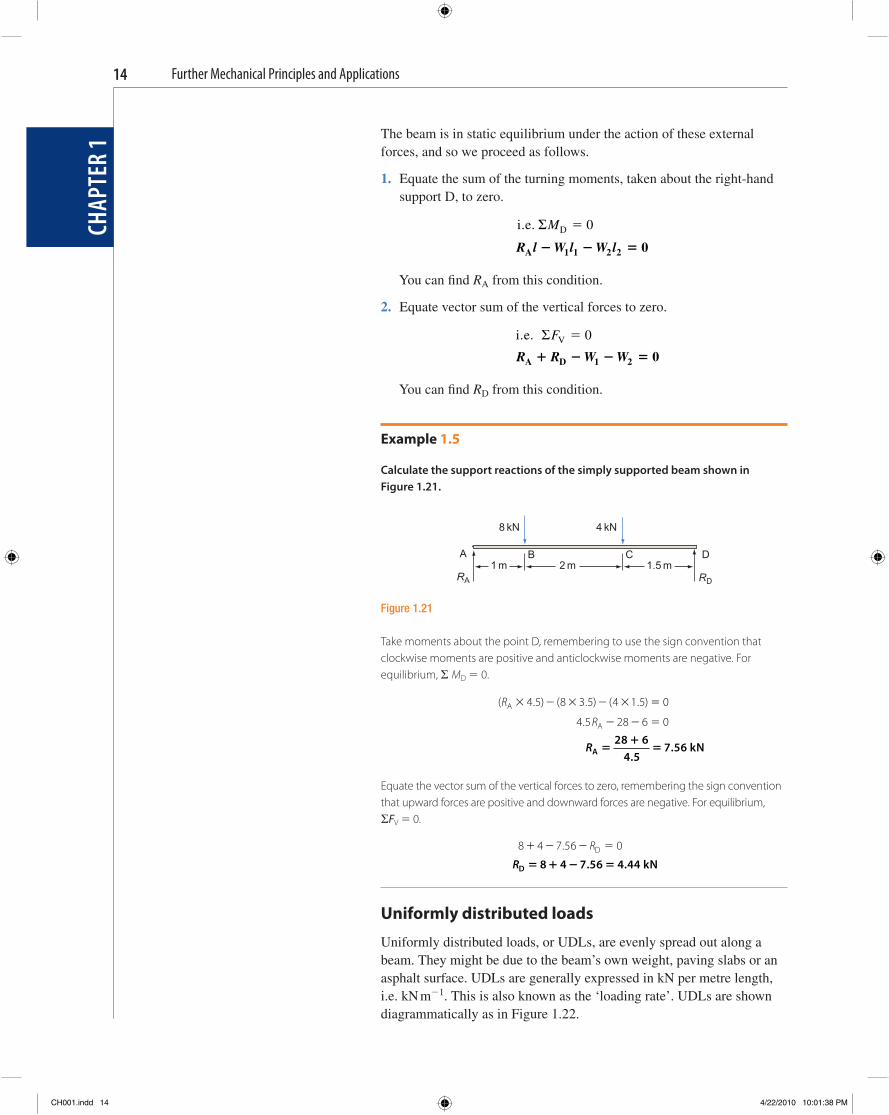
Example 1.5
Calculate the support reactions of the simply supported beam shown in Figure 1.21 .
8 kN 4 kN
A B C D1 m 2 m 1.5 m
RA RD
Figure 1.21
Take moments about the point D, remembering to use the sign convention that clockwise moments are positive and anticlockwise moments are negative. For equilibrium, � M D � 0.
( . ) . .
.
R
RA
A
( ) ( )� � � � � �
� � �
4 5 8 3 5 4 1 5 0
4 5 28 6 0
RA kN�
��
28 64 5
7 56.
.
Equate the vector sum of the vertical forces to zero, remembering the sign convention that upward forces are positive and downward forces are negative. For equilibrium, � F V � 0.
8 4 7 56 0� � � �. RD
RD kN� � � �8 4 7 56 4 44. .
Uniformly distributed loads
Uniformly distributed loads, or UDLs, are evenly spread out along a beam. They might be due to the beam ’ s own weight, paving slabs or an asphalt surface. UDLs are generally expressed in kN per metre length, i.e. kN m � 1 . This is also known as the ‘ loading rate ’ . UDLs are shown diagrammatically as in Figure 1.22 .
CH001.indd 14CH001.indd 14 4/22/2010 10:01:38 PM4/22/2010 10:01:38 PM
Further Mechanical Principles and Applications
CHAP
TER
1
15
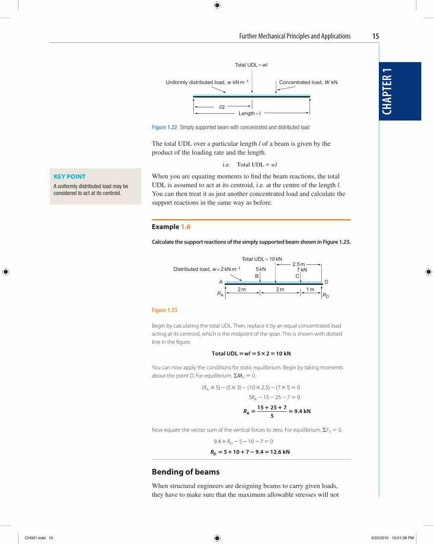
The total UDL over a particular length l of a beam is given by the product of the loading rate and the length.
i.e. Total UDL � wl
When you are equating moments to fi nd the beam reactions, the total UDL is assumed to act at its centroid, i.e. at the centre of the length l . You can then treat it as just another concentrated load and calculate the support reactions in the same way as before.
Example 1.6
Calculate the support reactions of the simply supported beam shown in Figure 1.23 .
Total UDL = wl
Uniformly distributed load, w kN m−1 Concentrated load, W kN
l/2Length = l
Figure 1.22 Simply supported beam with concentrated and distributed load
KEY POINT A uniformly distributed load may be considered to act at its centroid.
Total UDL = 10 kN2.5 m
Distributed load, w = 2 kN m−1 5 kN 7 kNB C
A D2 m 2 m 1 m
RA RD
Figure 1.23
Begin by calculating the total UDL. Then, replace it by an equal concentrated load acting at its centroid, which is the midpoint of the span. This is shown with dotted line in the fi gure.
Total UDL kN� � � � wl 5 2 10
You can now apply the conditions for static equilibrium. Begin by taking moments about the point D. For equilibrium, � M D � 0.
( ) .R
RA
A
( ) (10 ) (7 )� � � � � � � �
� � � �
5 5 3 2 5 1 0
5 15 25 7 0
RA kN�
� ��
15 25 75
9 4.
Now equate the vector sum of the vertical forces to zero. For equilibrium, � F V � 0.
9 4 5 10 7 0. � � � � �RD
RD kN� � � � �5 10 7 9 4 12 6. .
Bending of beams
When structural engineers are designing beams to carry given loads, they have to make sure that the maximum allowable stresses will not
CH001.indd 15CH001.indd 15 4/22/2010 10:01:38 PM4/22/2010 10:01:38 PM
Further Mechanical Principles and Applications
CHAP
TER
116
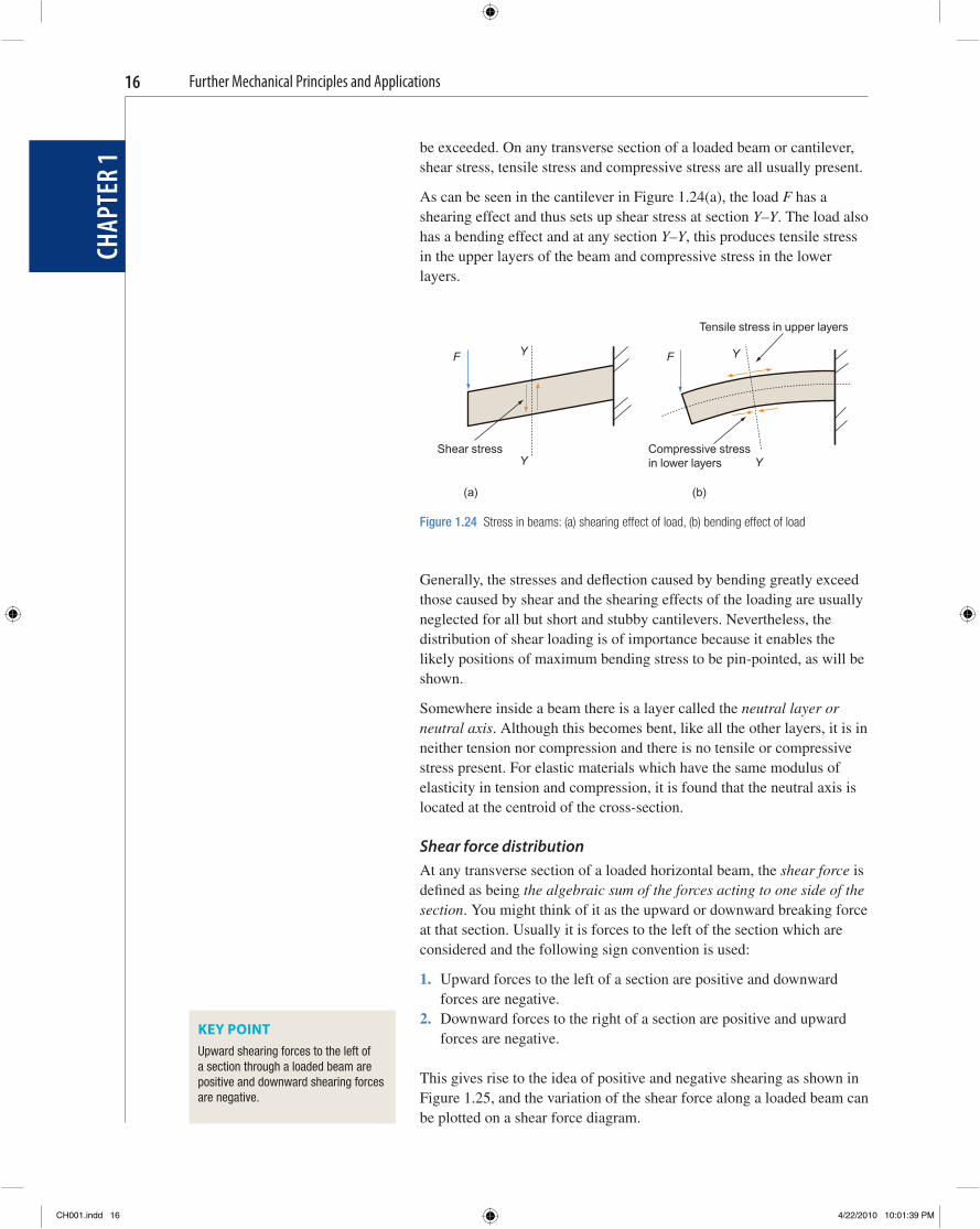
be exceeded. On any transverse section of a loaded beam or cantilever, shear stress, tensile stress and compressive stress are all usually present.
As can be seen in the cantilever in Figure 1.24(a) , the load F has a shearing effect and thus sets up shear stress at section Y–Y . The load also has a bending effect and at any section Y–Y , this produces tensile stress in the upper layers of the beam and compressive stress in the lower layers.
Tensile stress in upper layers
F F
Shear stress Compressive stressin lower layers
Y
Y Y
Y
(a) (b)
Figure 1.24 Stress in beams: (a) shearing effect of load, (b) bending effect of load
Generally, the stresses and defl ection caused by bending greatly exceed those caused by shear and the shearing effects of the loading are usually neglected for all but short and stubby cantilevers. Nevertheless, the distribution of shear loading is of importance because it enables the likely positions of maximum bending stress to be pin-pointed, as will be shown.
Somewhere inside a beam there is a layer called the neutral layer or neutral axis . Although this becomes bent, like all the other layers, it is in neither tension nor compression and there is no tensile or compressive stress present. For elastic materials which have the same modulus of elasticity in tension and compression, it is found that the neutral axis is located at the centroid of the cross-section.
Shear force distribution At any transverse section of a loaded horizontal beam, the shear force is defi ned as being the algebraic sum of the forces acting to one side of the section . You might think of it as the upward or downward breaking force at that section. Usually it is forces to the left of the section which are considered and the following sign convention is used:
1. Upward forces to the left of a section are positive and downward forces are negative.
2. Downward forces to the right of a section are positive and upward forces are negative.
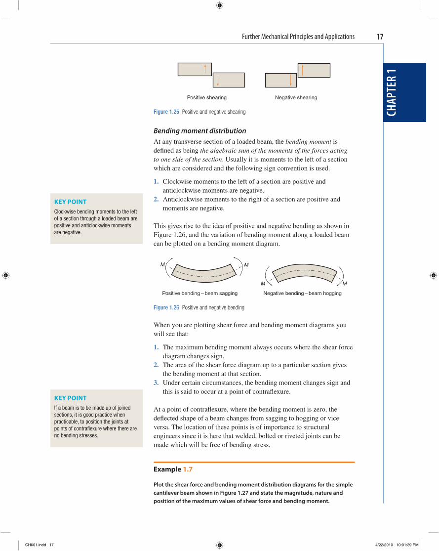
This gives rise to the idea of positive and negative shearing as shown in Figure 1.25 , and the variation of the shear force along a loaded beam can be plotted on a shear force diagram.
KEY POINT Upward shearing forces to the left of a section through a loaded beam are positive and downward shearing forces are negative.
CH001.indd 16CH001.indd 16 4/22/2010 10:01:39 PM4/22/2010 10:01:39 PM
Further Mechanical Principles and Applications
CHAP
TER
1
17
Bending moment distribution At any transverse section of a loaded beam, the bending moment is defi ned as being the algebraic sum of the moments of the forces acting to one side of the section . Usually it is moments to the left of a section which are considered and the following sign convention is used.
1. Clockwise moments to the left of a section are positive and anticlockwise moments are negative.
2. Anticlockwise moments to the right of a section are positive and moments are negative.
This gives rise to the idea of positive and negative bending as shown in Figure 1.26 , and the variation of bending moment along a loaded beam can be plotted on a bending moment diagram.
Positive shearing Negative shearing
Figure 1.25 Positive and negative shearing
M M
M M
Positive bending – beam sagging Negative bending – beam hogging
Figure 1.26 Positive and negative bending
When you are plotting shear force and bending moment diagrams you will see that:
1. The maximum bending moment always occurs where the shear force diagram changes sign.
2. The area of the shear force diagram up to a particular section gives the bending moment at that section.
3. Under certain circumstances, the bending moment changes sign and this is said to occur at a point of contrafl exure.
At a point of contrafl exure, where the bending moment is zero, the defl ected shape of a beam changes from sagging to hogging or vice versa. The location of these points is of importance to structural engineers since it is here that welded, bolted or riveted joints can be made which will be free of bending stress.
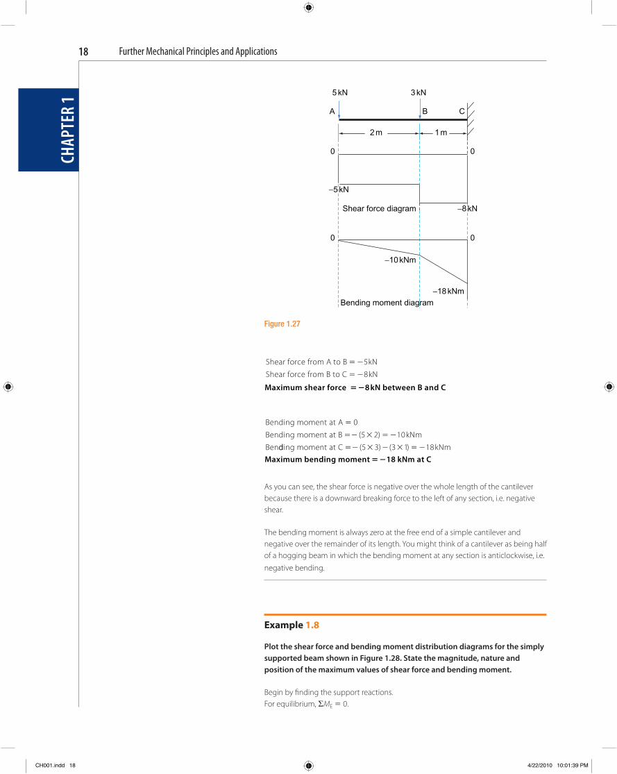
Example 1.7
Plot the shear force and bending moment distribution diagrams for the simple cantilever beam shown in Figure 1.27 and state the magnitude, nature and position of the maximum values of shear force and bending moment.
KEY POINT Clockwise bending moments to the left of a section through a loaded beam are positive and anticlockwise moments are negative.
KEY POINT If a beam is to be made up of joined sections, it is good practice when practicable, to position the joints at points of contrafl exure where there are no bending stresses.
CH001.indd 17CH001.indd 17 4/22/2010 10:01:39 PM4/22/2010 10:01:39 PM
Further Mechanical Principles and Applications
CHAP
TER
118
Shear force from A to B kN
Shear force from B to C kN
� �
� �
5
8
Maximum shear force kN between B and C��8
Bending moment at A
Bending moment at B kNm
Ben
�
� � � � �
0
5 2 10( )
dding moment at C kNm� � � � � � �( ) ( )5 3 3 1 18
Maximum bending moment kNm at C��18
As you can see, the shear force is negative over the whole length of the cantilever because there is a downward breaking force to the left of any section, i.e. negative shear.
The bending moment is always zero at the free end of a simple cantilever and negative over the remainder of its length. You might think of a cantilever as being half of a hogging beam in which the bending moment at any section is anticlockwise, i.e.
negative bending.
Example 1.8
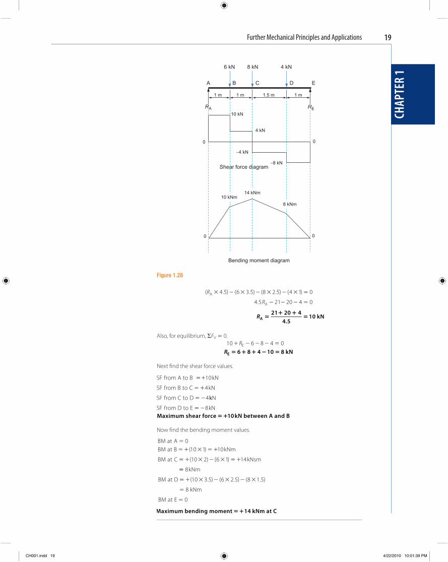
Plot the shear force and bending moment distribution diagrams for the simply supported beam shown in Figure 1.28 . State the magnitude, nature and position of the maximum values of shear force and bending moment.
Begin by fi nding the support reactions. For equilibrium, � M E � 0.
Figure 1.27
5 kN 3 kN
A B C
2 m 1 m
0 0
0
−5 kN
Shear force diagram −8 kN
0
−10 kNm
−18 kNmBending moment diagram
CH001.indd 18CH001.indd 18 4/22/2010 10:01:39 PM4/22/2010 10:01:39 PM
Further Mechanical Principles and Applications
CHAP
TER
1
19
( . ) ( . ) ( . ) ( )
.
R
RA
A
� � � � � � � �
� � � �
4 5 6 3 5 8 2 5 4 1 0
4 5 21 20 4 0
RA kN�
� ��
21 20 44 5
10.
Also, for equilibrium, � F V � 0. 10 6 8 4 0� � � � �RE RE kN� � � � �6 8 4 10 8
Next fi nd the shear force values.
SF from A to B kN
SF from B to C kN
SF from C to D
� �
� �
� �
10
4
4kkN
SF from D to E kN� �8 Maximum shear force kN between A and B��10
Now fi nd the bending moment values.
BM at ABM at B kNm
BM at C kNsm
�
� � � � �
� � � � � � �
010 1 10
10 2 6 1 14
( )
( ) ( )
��
� � � � � � �
�
�
8
10 3 5 6 2 5 8 1 5
0
kNm
BM at D
8 kNm
BM at E
( . ) ( . ) ( . )
Maximum bending moment kNm at C��14
6 kN 8 kN 4 kN
A B C D E
0 0
Shear force diagram
Bending moment diagram
00
RA
1 m 1 m 1.5 m 1 m
10 kN
4 kN
−4 kN
−8 kN
14 kNm 10 kNm
8 kNm
RE
Figure 1.28
CH001.indd 19CH001.indd 19 4/22/2010 10:01:39 PM4/22/2010 10:01:39 PM
Further Mechanical Principles and Applications20
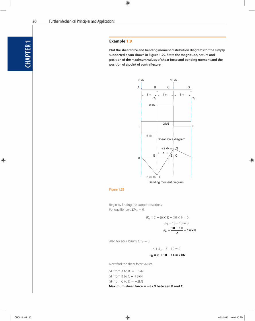
Example 1.9
Plot the shear force and bending moment distribution diagrams for the simply supported beam shown in Figure 1.29 . State the magnitude, nature and position of the maximum values of shear force and bending moment and the position of a point of contrafl exure.
6 kN 10 kN
A B C D
1 m 1 m 1 mRB RD
+8 kN
0 0 −2 kN
−6 kNShear force diagram
+2 kN m Gx
0B E
0
−6 kN m
Bending moment diagram
C
F
Figure 1.29
Begin by fi nding the support reactions. For equilibrium, � M D � 0.
( ) ( ) ( )R
RB
B
� � � � � �
� � �
2 6 3 10 1 0
2 18 10 0
RB kN�
��
18 102
14
Also, for equilibrium, � F V � 0.
14 6 10 0� � � �RD
RD kN� � � �6 10 14 2
Next fi nd the shear force values.
SF from A to B kN
SF from B to C kN
SF from C to D k
� �
� �
� �
6
8
2 NN
Maximum shear force kN between B and C��8
CHAP
TER
1
CH001.indd 20CH001.indd 20 4/22/2010 10:01:40 PM4/22/2010 10:01:40 PM
Further Mechanical Principles and Applications
CHAP
TER
1
21
Now fi nd the bending moment values.
BM at A
BM at B kNm
BM at C kNm
BM a
�
� � � � �
� � � � � � �
0
6 1 6
6 2 14 1 2
( )
( ) ( )
tt D � 0
Maximum bending moment kNm at B��6
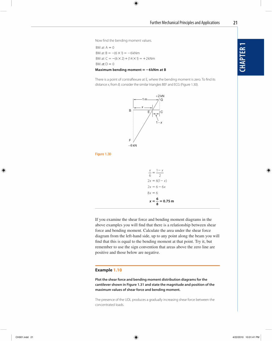
There is a point of contrafl exure at E, where the bending moment is zero. To fi nd its distance x , from B , consider the similar triangles BEF and ECG ( Figure 1.30 ).
+2 kN
1 m G
xB
1 − x
F
−6 kN
CE
Figure 1.30
x x
x x
x x
x
61
22 6 1
2 6 6
8 6
��
� �
� �
�
( )
x � �
68
0 75. m
If you examine the shear force and bending moment diagrams in the above examples you will fi nd that there is a relationship between shear force and bending moment. Calculate the area under the shear force diagram from the left-hand side, up to any point along the beam you will fi nd that this is equal to the bending moment at that point. Try it, but remember to use the sign convention that areas above the zero line are positive and those below are negative.
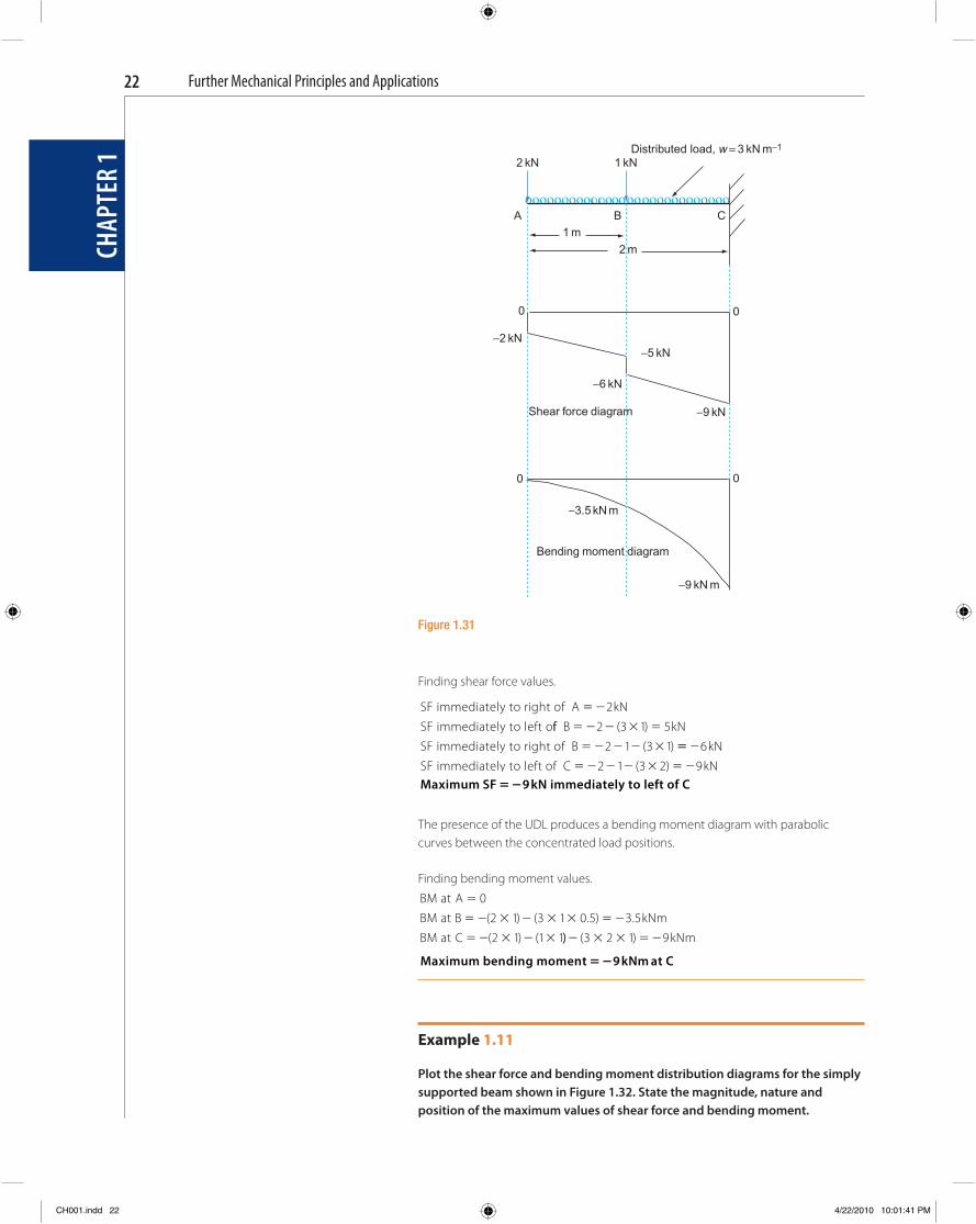
Example 1.10
Plot the shear force and bending moment distribution diagrams for the cantilever shown in Figure 1.31 and state the magnitude and position of the maximum values of shear force and bending moment.
The presence of the UDL produces a gradually increasing shear force between the concentrated loads.
CH001.indd 21CH001.indd 21 4/22/2010 10:01:41 PM4/22/2010 10:01:41 PM
Further Mechanical Principles and Applications22
Finding shear force values.
SF immediately to right of A kN
SF immediately to left o
� �2
ff B kN
SF immediately to right of B
� � � � �
� � � � �
2 3 1 5
2 1 3 1
( )
( ) �� �
� � � � � � �
6
2 1 3 2 9
kN
SF immediately to left of C kN( )
Maximum SF kN immediately to left of C��9
The presence of the UDL produces a bending moment diagram with parabolic curves between the concentrated load positions.
Finding bending moment values.
BM at A
BM at B kNm
BM at C
�
� � � � � � � �
� � � � �
0
2 1 3 1 0 5 3 5
2 1 1 1
( ) ( . ) .
( ) ( )) ( )� � � � �3 2 1 9kNm
Maximum bending moment kNm at C��9
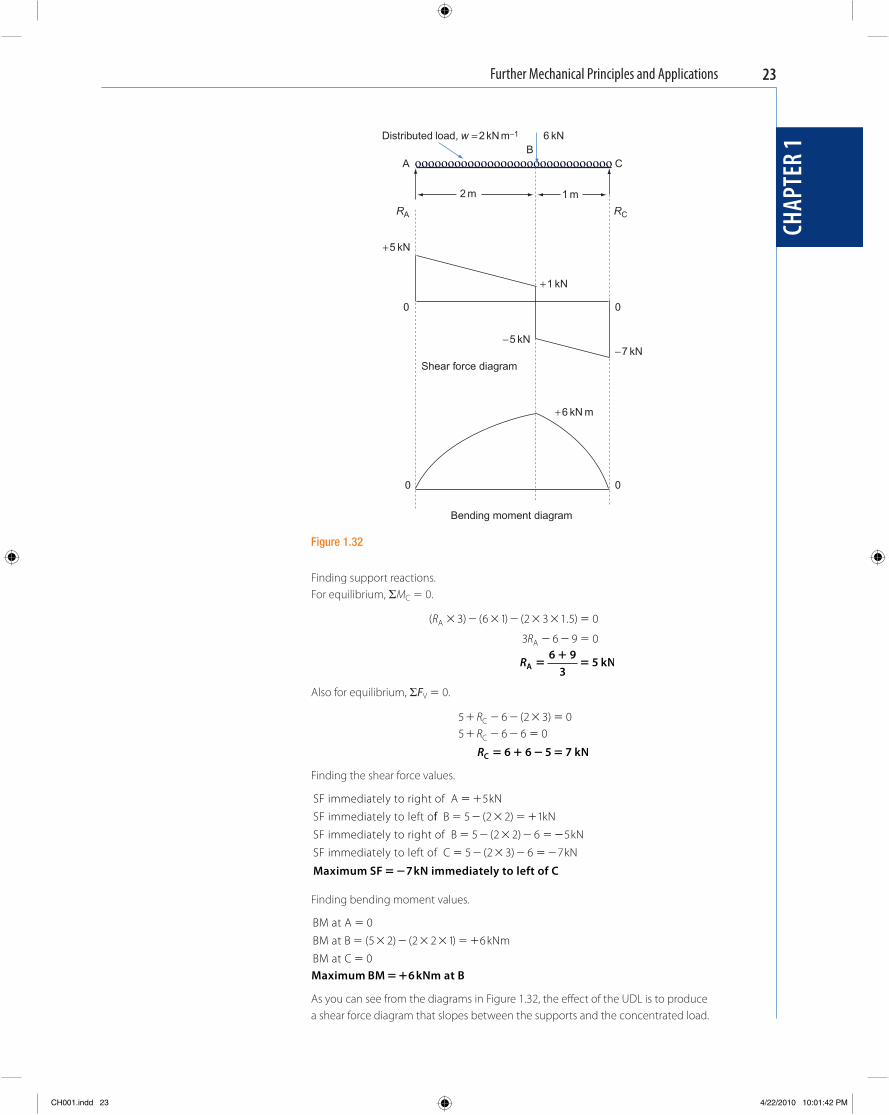
Example 1.11
Plot the shear force and bending moment distribution diagrams for the simply supported beam shown in Figure 1.32 . State the magnitude, nature and position of the maximum values of shear force and bending moment.
Distributed load, w = 3 kN m−1
2 kN 1 kN
A B C1 m
2 m
0 0
0
−2 kN−5 kN
−6 kN
Shear force diagram −9 kN
0
−3.5 kN m
Bending moment diagram
−9 kN m
Figure 1.31
CHAP
TER
1
CH001.indd 22CH001.indd 22 4/22/2010 10:01:41 PM4/22/2010 10:01:41 PM
Further Mechanical Principles and Applications
CHAP
TER
1
23
Finding support reactions. For equilibrium, � M C � 0.
( ) ( ) ( . )R
RA
A
� � � � � � �
� � �
3 6 1 2 3 1 5 0
3 6 9 0
RA kN�
��
6 93
5
Also for equilibrium, � F V � 0.
5 6 2 3 05 6 6 0
� � � � �
� � � �
RR
C
C
( )
RC kN� � � �6 6 5 7 Finding the shear force values.
SF immediately to right of A kN
SF immediately to left o
� �5
ff B kN
SF immediately to right of B
� � � � �
� � � � �
5 2 2 1
5 2 2 6
( )
( ) ��
� � � � � �
5
5 2 3 6 7
kN
SF immediately to left of C kN( )
Maximum SF kN immediately to left of C��7
Finding bending moment values.
BM at A
BM at B kNm
BM at C
�
� � � � � � �
�
0
5 2 2 2 1 6
0
( ) ( )
Maximum BM kNm at B��6 As you can see from the diagrams in Figure 1.32 , the eff ect of the UDL is to produce a shear force diagram that slopes between the supports and the concentrated load.
Distributed load, w = 2 kN m−1 6 kNB
A C
2 m 1 m
+5 kN
+1 kN
0 0
−5 kN−7 kN
Shear force diagram
+6 kN m
0 0
Bending moment diagram
RCRA
Figure 1.32
CH001.indd 23CH001.indd 23 4/22/2010 10:01:42 PM4/22/2010 10:01:42 PM
Further Mechanical Principles and Applications
CHAP
TER
124
Its slope 2 kN m � 1 , which is the UDL rate. The eff ect on the bending moment diagram
is to produce parabolic curves between the supports and the concentrated load.
? Test your knowledge 1.3 1. What is the difference between an active and a reactive load? 2. How do you defi ne the shear force at any point on a loaded beam? 3. How do you defi ne the bending moment at any point on a loaded
beam? 4. What is a point of contrafl exure?
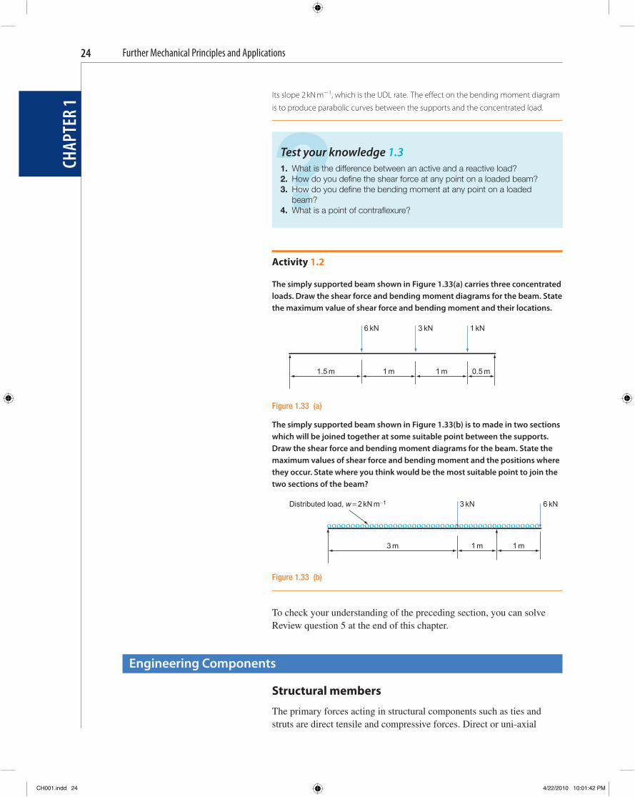
Activity 1.2
The simply supported beam shown in Figure 1.33(a) carries three concentrated loads. Draw the shear force and bending moment diagrams for the beam. State the maximum value of shear force and bending moment and their locations.
To check your understanding of the preceding section, you can solve Review question 5 at the end of this chapter.
Engineering Components
Structural members
The primary forces acting in structural components such as ties and struts are direct tensile and compressive forces. Direct or uni-axial
The simply supported beam shown in Figure 1.33(b) is to made in two sections which will be joined together at some suitable point between the supports. Draw the shear force and bending moment diagrams for the beam. State the maximum values of shear force and bending moment and the positions where they occur. State where you think would be the most suitable point to join the two sections of the beam?
6 kN 3 kN 1 kN
1.5 m 1 m 1 m 0.5 m
Figure 1.33 (a)
Distributed load, w = 2 kN m−1 3 kN 6 kN
3 m 1 m 1 m
Figure 1.33 (b)
CH001.indd 24CH001.indd 24 4/22/2010 10:01:42 PM4/22/2010 10:01:42 PM
Further Mechanical Principles and Applications
CHAP
TER
1
25
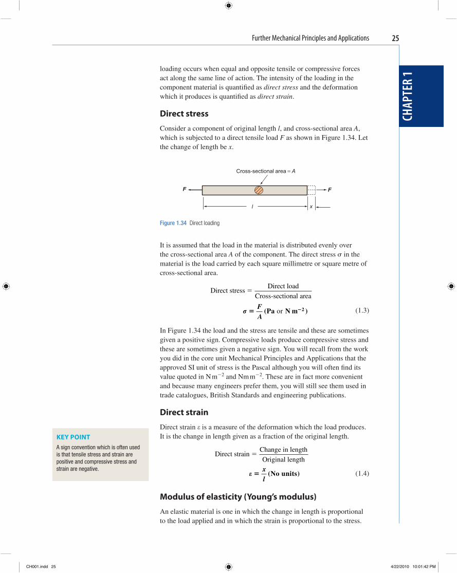
It is assumed that the load in the material is distributed evenly over the cross-sectional area A of the component. The direct stress � in the material is the load carried by each square millimetre or square metre of cross-sectional area.
Direct stress
Direct load
Cross-sectional area�
� � �F
A( )Pa N mor 2 (1.3)
In Figure 1.34 the load and the stress are tensile and these are sometimes given a positive sign. Compressive loads produce compressive stress and these are sometimes given a negative sign. You will recall from the work you did in the core unit Mechanical Principles and Applications that the approved SI unit of stress is the Pascal although you will often fi nd its value quoted in N m � 2 and Nm m � 2 . These are in fact more convenient and because many engineers prefer them, you will still see them used in trade catalogues, British Standards and engineering publications.
Direct strain
Direct strain � is a measure of the deformation which the load produces. It is the change in length given as a fraction of the original length.
Direct strain
Change in length
Original length�
� �
xl
( )No units (1.4)
Modulus of elasticity (Young ’ s modulus)
An elastic material is one in which the change in length is proportional to the load applied and in which the strain is proportional to the stress.
Cross-sectional area = A
F F
l x
Figure 1.34 Direct loading
KEY POINT A sign convention which is often used is that tensile stress and strain are positive and compressive stress and strain are negative.
loading occurs when equal and opposite tensile or compressive forces act along the same line of action. The intensity of the loading in the component material is quantifi ed as direct stress and the deformation which it produces is quantifi ed as direct strain .
Direct stress
Consider a component of original length l , and cross-sectional area A , which is subjected to a direct tensile load F as shown in Figure 1.34 . Let the change of length be x .
CH001.indd 25CH001.indd 25 4/22/2010 10:01:42 PM4/22/2010 10:01:42 PM
Further Mechanical Principles and Applications
CHAP
TER
126
Substituting the expressions for stress and strain from equations (1.3) and (1.4) gives an alternative formula:
E
F
Ax
l
�
E
FA
lx
� � (1.6)
Factor of safety
Engineering components should be designed so that the working stress which they are likely to encounter is well below the ultimate stress at which failure occurs.
Factor of safety
Ultimate stressWorking stress
�
(1.7)
A factor of safety of at least 2 is generally applied for static structures. This ensures that the working stress will be no more than half of that at which failure occurs. Much lower factors of safety are applied in aircraft design where weight is at a premium and with some of the major components it is likely that failure will eventually occur due to metal fatigue. These are rigorously tested at the prototype stage to predict their working life and replaced periodically in service well before this period has elapsed.
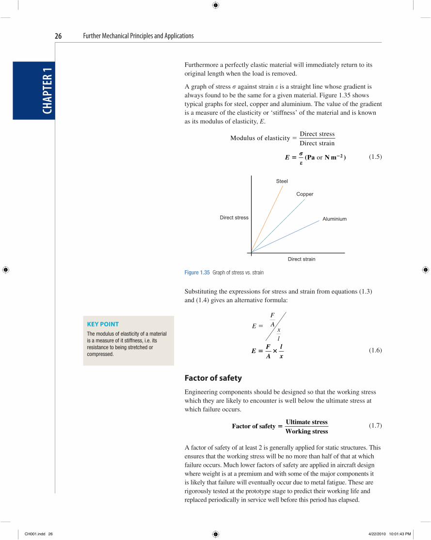
Steel
Copper
Direct stress Aluminium
Direct strain
Figure 1.35 Graph of stress vs. strain
KEY POINT The modulus of elasticity of a material is a measure of it stiffness, i.e. its resistance to being stretched or compressed.
Furthermore a perfectly elastic material will immediately return to its original length when the load is removed.
A graph of stress � against strain � is a straight line whose gradient is always found to be the same for a given material. Figure 1.35 shows typical graphs for steel, copper and aluminium. The value of the gradient is a measure of the elasticity or ‘ stiffness ’ of the material and is known as its modulus of elasticity, E .
Modulus of elasticity
Direct stress
Direct strain�
E � ��
�( )Pa N mor 2 (1.5)
CH001.indd 26CH001.indd 26 4/22/2010 10:01:43 PM4/22/2010 10:01:43 PM
Further Mechanical Principles and Applications
CHAP
TER
1
27
Example 1.12
A strut of diameter 25 mm and length 2 m carries an axial load of 20 kN. The ultimate compressive stress of the material is 350 MPa and its modulus of elasticity is 150 GPa. Find (a) the compressive stress in the material, (b) the factor of safety in operation, (c) the change in length of the strut.
(a) Finding cross-sectional area of strut.
A
d� �
�� �2 2
40 0254.
A � � �491 10 6 2m Finding compressive stress.
� � �
�
� �
FA
20 10491 10
3
6
� � �40 7 10 40 76. or .Pa MPa (b) Finding factor of safety in operation.
Factor of safety
Ultimate stressWorking stress
� ��350 10
40 7
6
. ��106
Factor of safety � 8 6. (c) Finding compressive strain.
E
E
�
� ��
�
��
�� 40 7 10
150 10
6
9
.
� � � �271 10 6
Finding change in length.
�
�
�
� � � ��
xl
x l ( )271 10 26
x � � �0 543 10 0 5433. .m or mm
? Test your knowledge 1.4 1. What is meant by uni-axial loading? 2. What is the defi nition of an elastic material? 3. A tie bar of cross-sectional area 50 mm 2 carries a load of 10 kN. What is
the tensile stress in the material measured in Pascals? 4. If the ultimate tensile stress at which failure occurs in a material
is 550 MPa and a factor of safety of 4 is to apply, what will be the allowable working stress?
Activity 1.3 A tube of length 1.5 m has an inner diameter 50 mm and wall thickness of 6 mm. When subjected to a direct tensile load of 75 kN the length is seen to increase by 0.55 mm. Determine (a) the tensile stress in the material, (b) the factor of safety in operation if the ultimate tensile strength of the material is 350 MPa, (c) the modulus of elasticity of the material.
CH001.indd 27CH001.indd 27 4/22/2010 10:01:43 PM4/22/2010 10:01:43 PM
Further Mechanical Principles and Applications
CHAP
TER
128
Thermal loading
Most materials expand when their temperature rises. This is certainly true of the more commonly used metals in engineering and the effect is measured as the linear expansivity of a material. It is defi ned as the change in length per unit of length per degree of temperature change and its symbol is � . It is also known as the coeffi cient of linear expansion and its units are °C � 1 .
To fi nd the change in length x of a component of original length l and linear expansivity � when its temperature changes by t °C, we use the formula,
x l t� � (1.8)
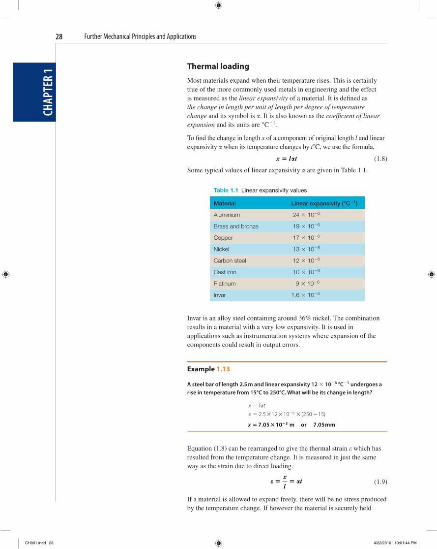
Some typical values of linear expansivity � are given in Table 1.1 .
Table 1.1 Linear expansivity values
Material Linear expansivity ( ° C � 1 )
Aluminium 24 � 10 � 6
Brass and bronze 19 � 10 � 6
Copper 17 � 10 � 6
Nickel 13 � 10 � 6
Carbon steel 12 � 10 � 6
Cast iron 10 � 10 � 6
Platinum 9 � 10 � 6
Invar 1.6 � 10 � 6
Invar is an alloy steel containing around 36% nickel. The combination results in a material with a very low expansivity. It is used in applications such as instrumentation systems where expansion of the components could result in output errors.
Example 1.13
A steel bar of length 2.5 m and linear expansivity 12 � 10 � 6 °C � 1 undergoes a rise in temperature from 15°C to 250°C. What will be its change in length?
x l t
x
�
� � � � ��
�2 5 12 10 250 156. ( )
x � � �7 05 10 7 053. .m or mm
Equation (1.8) can be rearranged to give the thermal strain � which has resulted from the temperature change. It is measured in just the same way as the strain due to direct loading.
� �� �
xl
t (1.9)
If a material is allowed to expand freely, there will be no stress produced by the temperature change. If however the material is securely held
CH001.indd 28CH001.indd 28 4/22/2010 10:01:44 PM4/22/2010 10:01:44 PM
Further Mechanical Principles and Applications
CHAP
TER
1
29
and the change in length is prevented, thermal stress � will be induced. The above equation gives the virtual mechanical strain to which it is proportional and if the modulus of elasticity E for the material is known, the value of the stress can be calculated as follows:
E
t� �
��
��
� �� E t (1.10)
You will see from the above equation that thermal stress depends only on the material properties and the temperature change.
Example 1.14
A steam pipe made from steel is fi tted at a temperature of 20°C. If expansion is prevented, what will be the compressive stress in the material when steam at a temperature of 150°C fl ows through it? Take � � 12 � 10 � 6 °C � 1 and E � 200 GN m � 2 .
� �
�
�
� � � � � ��
E t
200 10 12 10 150 209 6 ( )
� � �312 10 3126 Pa or MPa
You should note that this is quite a high level of stress which could very easily cause the pipe to buckle. This is why expansion loops and expansion joints are included in steam pipe systems, to reduce the stress to an acceptably low level.
Combined direct and thermal loading
It is of course quite possible to have a loaded component which is rigidly held and which also undergoes temperature change. This often happens with aircraft components and with components in process plants. Depending on whether the temperature rises or falls, the stress in the component may increase or decrease.
When investigating the effects of combined direct and thermal stress it is useful to adopt the sign convention that tensile stress and strain are positive and compressive stress and strain are negative. The resultant strain and stress is the algebraic sum of the direct and thermal values.
Resultant stress Direct stress Thermal stress
D T
� �
� �� � �
� �� �
FA
E t
(1.11)
Resultant strain Direct strain Thermal strain
D T
� �
� �� � �
� �� �
xl
t
(1.12)
Having calculated either the resultant stress or the resultant strain, the other can be found from the modulus of elasticity of the material.
KEY POINT Thermal stress is independent of the dimensions of a restrained component. It is dependent only on its modulus of elasticity, its linear expansivity and the temperature change which takes place.
KEY POINT Residual thermal stresses are sometimes present in cast and forged components which have cooled unevenly. They can cause the component to become distorted when material is removed during machining. Residual thermal stresses can be removed by heat treatment and this will be described in Chapter 4.
CH001.indd 29CH001.indd 29 4/22/2010 10:01:44 PM4/22/2010 10:01:44 PM
Further Mechanical Principles and Applications
CHAP
TER
130
Modulus of elasticity
Resultant stress
Resultant strain�
E �
�
� (1.13)
Example 1.15
A rigidly held tie bar in a heating chamber has a diameter of 60 mm and is tensioned to a load of 150 kN at a temperature of 15°C. What is the initial stress in the bar and what will be the resultant stress when the temperature in the chamber has risen to 50°C?
Take E � 200 GN m � 2 and � � 12 � 10 � 6 °C � 1 .
Note : The initial tensile stress will be positive but the thermal stress will be compressive and negative. It will thus have a cancelling eff ect.
Finding cross-sectional area.
A
d�
�� �2 2
40 064
=.
A � � �2 83 10 3 2. m
Finding initial direct tensile stress at 15°C.
�D � � �
�
� �
FA
150 102 83 10
3
3.
� D Pa or MPa�� � �53 0 10 53 06. .
Finding thermal compressive stress at 50°C.
� �T � � � � � � � ��E t 200 10 12 10 50 159 6 ( )
� T Pa or MPa�� � ��84 0 10 84 06. .
Finding resultant stress at 50°C.
� � �� � � � � �D T 53 0 84 0. ( . )
� ��31 0. MPa i.e. the initial tensile stress has been cancelled out during the temperature rise and the fi nal resultant stress is compressive.
? Test your knowledge 1.5 1. How do you defi ne the linear expansivity of a material? 2. If identical lengths of steel and aluminium bar undergo the same
temperature rise, which one will expand the most? 3. What effect do the dimensions of a rigidly clamped component have on
the thermal stress caused by temperature change?
Activity 1.4 A rigidly fi xed strut in a refrigeration system carries a compressive load of 50 kN when assembled at a temperature of 20°C. The initial length of the strut is 0.5 m and its diameter is 30 mm. Determine the initial stress in the strut
CH001.indd 30CH001.indd 30 4/22/2010 10:01:44 PM4/22/2010 10:01:44 PM
Further Mechanical Principles and Applications
CHAP
TER
1
31
and the amount of compression under load. At what operating temperature will the stress in the material have fallen to zero? Take E � 150 GN m � 2 and � � 16 � 10 � 6 .
To check your understanding of the preceding section, you can solve Review questions 6–10 at the end of this chapter.
Compound members
Engineering components are sometimes fabricated from two different materials. Materials joined end to end form series compound members. Materials which are sandwiched together or contained one within another form parallel compound members.
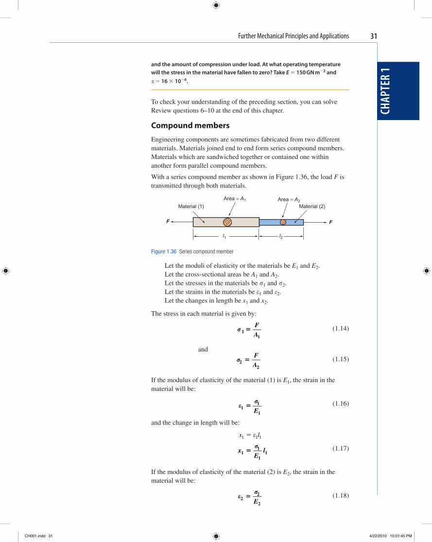
With a series compound member as shown in Figure 1.36 , the load F is transmitted through both materials.
Area = A1 Area = A2Material (1) Material (2)
F F
l1 l2
Figure 1.36 Series compound member
Let the moduli of elasticity or the materials be E 1 and E 2 . Let the cross-sectional areas be A 1 and A 2 . Let the stresses in the materials be � 1 and � 2 . Let the strains in the materials be � 1 and � 2 . Let the changes in length be x 1 and x 2 .
The stress in each material is given by:
� 1
1
�FA
(1.14)
and
�2
2
�FA
(1.15)
If the modulus of elasticity of the material (1) is E 1 , the strain in the material will be:
�
�1
1
1
�E
(1.16)
and the change in length will be:
x l1 1 1� �
x1 �
�1
11E
l (1.17)
If the modulus of elasticity of the material (2) is E 2 , the strain in the material will be:
�
�2
2
2
�E
(1.18)
CH001.indd 31CH001.indd 31 4/22/2010 10:01:45 PM4/22/2010 10:01:45 PM
Further Mechanical Principles and Applications
CHAP
TER
132
and the change in length will be:
x l2 2 2� �
x2 �
�2
22E
l
(1.19)
The total change in length will thus be:
x x x� �1 2
x
El
El� �
� �1
11
2
22
(1.20)
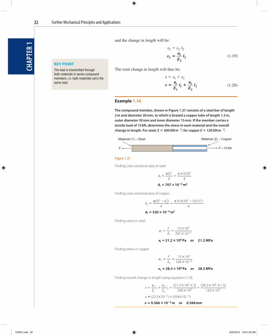
Example 1.16
The compound member, shown in Figure 1.37 consists of a steel bar of length 2 m and diameter 30 mm, to which is brazed a copper tube of length 1.5 m, outer diameter 30 mm and inner diameter 15 mm. If the member carries a tensile load of 15 kN, determine the stress in each material and the overall change in length. For steel, E � 200 GN m � 2 , for copper E � 120 GN m � 2 .
KEY POINT The load is transmitted through both materials in series compound members, i.e. both materials carry the same load.
Material (1) – Steel Material (2) – Copper
F F = 15 kN
Figure 1.37
Finding cross-sectional area of steel.
A
Dl1
2 2
40 034
� ��� � .
A16 2707 10� � � m
Finding cross-sectional area of copper.
A
D d2
12
22 2 2
40 03 0 015
4�
��
� �� �( ) ( . . )
A16 2530 10� � � m
Finding stress in steel.
�1
1
3
6
15 10707 10
� ��
� �
FA
�1621 2 10 21 2� �. .Pa or MPa
Finding stress in copper.
�2
2
3
6
15 10530 10
� ��
� �
FA
�1
628 3 10 28 3� �. .Pa or MPa
Finding overall change in length using equation (1.19).
xE
lE
l
x
� � �� �
��
� �
�
� �1
11
2
22
6
9
6
9
21 2 10 2200 10
28 3 10 1 5120 10
( . ) ( . . )
�� � � �� �( ) ( )212 10 354 106 6
x � � �0 566 10 0 5663. .m or mm
CH001.indd 32CH001.indd 32 4/22/2010 10:01:45 PM4/22/2010 10:01:45 PM
Further Mechanical Principles and Applications
CHAP
TER
1
33
With parallel compound members, the loads in each material will most likely be different but when added together they will equal the external load. The change in length of each material will be the same. When you are required to fi nd the stress in each material, this information enables you to write down two equations, each of which contains the unknown stresses. You can then solve these by substitution and use one of the stress values to fi nd the common change in length.
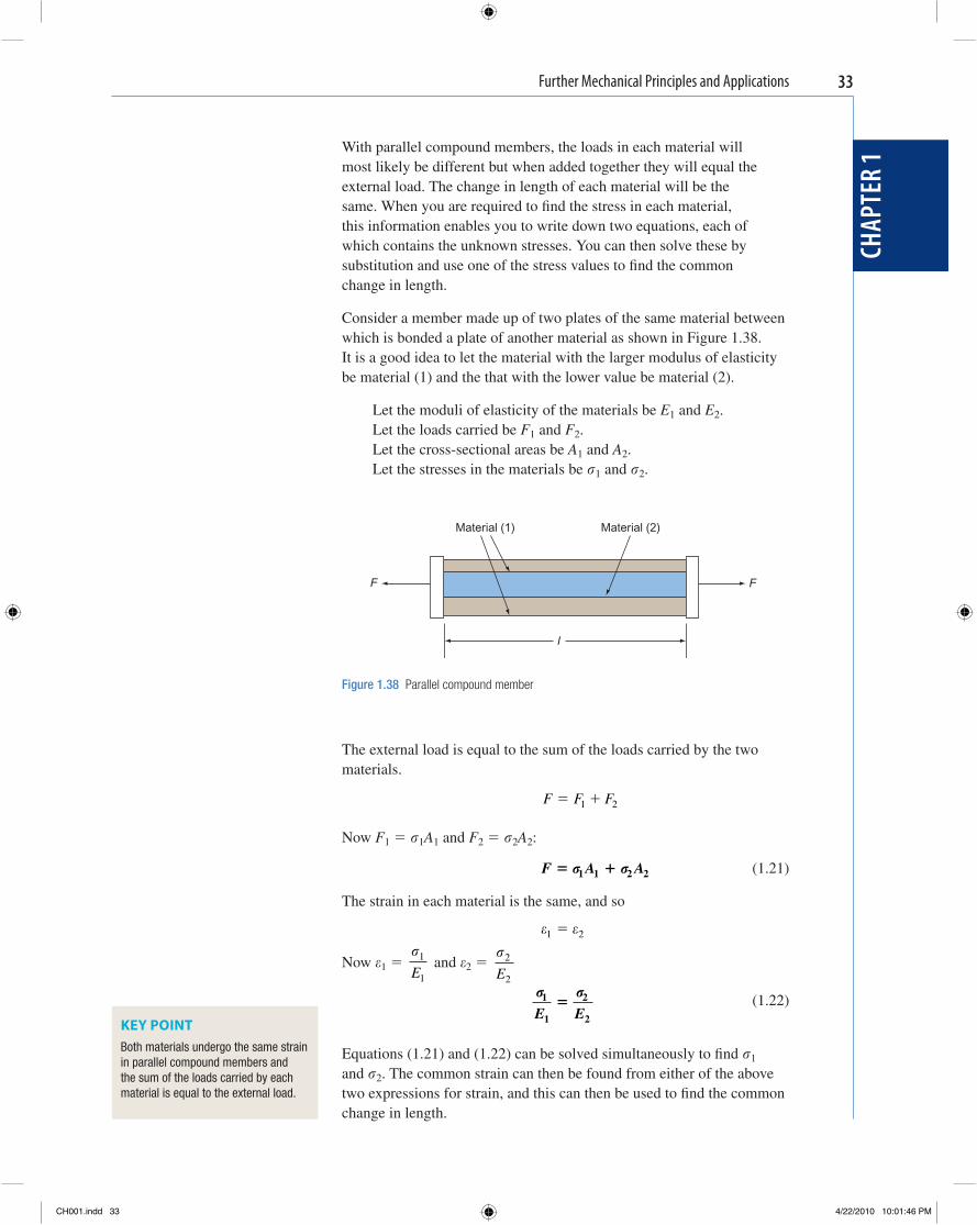
Consider a member made up of two plates of the same material between which is bonded a plate of another material as shown in Figure 1.38 . It is a good idea to let the material with the larger modulus of elasticity be material (1) and the that with the lower value be material (2).
Let the moduli of elasticity of the materials be E 1 and E 2 . Let the loads carried be F 1 and F 2 . Let the cross-sectional areas be A 1 and A 2 . Let the stresses in the materials be � 1 and � 2 .
Material (1) Material (2)
F F
l
Figure 1.38 Parallel compound member
The external load is equal to the sum of the loads carried by the two materials.
F F F� �1 2
Now F 1 � � 1 A 1 and F 2 � � 2 A 2 :
F A A� �� �1 1 2 2 (1.21)
The strain in each material is the same, and so
� �1 2�
Now � 1 � �1
1E and � 2 �
�2
2E
� �1
1
2
2E E�
(1.22)
Equations (1.21) and (1.22) can be solved simultaneously to fi nd � 1 and � 2 . The common strain can then be found from either of the above two expressions for strain, and this can then be used to fi nd the common change in length.
KEY POINT Both materials undergo the same strain in parallel compound members and the sum of the loads carried by each material is equal to the external load.
CH001.indd 33CH001.indd 33 4/22/2010 10:01:46 PM4/22/2010 10:01:46 PM

Further Mechanical Principles and Applications
CHAP
TER
134
Example 1.17
A concrete column 200 mm square is reinforced by nine steel rods of diameter 20 mm. The length of the column is 3 m and it is required to support an axial compressive load of 500 kN. Find the stress in each material and the change in length of the column under load. For steel E � 200 GN m � 2 and for concrete, E � 20 GN m � 2 .
Because the steel has the higher modulus of elasticity, let it be material (1) and the concrete be material (2).
Begin by fi nding the cross-sectional areas of the two materials.
A
d1
2 29
49
0 024
� � � ��� � .
A13 22 83 10� � �. m
A A2 130 2 0 2 0 04 2 83 10� � � � � � �( . . ) . ( . )
A23 237 2 10� � �. m
Now equate the external force to the sum of the forces in the two materials using equation (1.21).
F A A� �
� � � � �� �
� �
� �1 1 2 2
3 31
32500 10 2 83 10 37 2 10( . ) ( . )
This can be simplifi ed by dividing both sides by 10 � 3 :
500 10 2 83 37 261 2� � �. .� � (1)
Now equate the strains in each material using equation (1.21):
� �
� �
� �
1
1
2
2
11
22
1
9
9 2200 1020 10
E E
EE
�
�
��
��
� �1 210� (2)
Substitute in (1) for � 1 :
500 10 2 83 10 37 2
500 10 28 3 37 2 65 5
50
62 2
62 2 2
2
� � �
� � � �
�
. ( ) .
. . .
� �
� � �
�00 1065 5
6�
.
�2
67 63 10 7 63� �. .Pa or MPa
Finding � 1 from (2):
�1 10 7 63 76 3� � �. . MPa
Now fi nd the common strain using the stress and modulus of elasticity for material (2):
�
�� �
�
�2
2
6
9
7 63 1020 10E.
� � � �382 10 6
CH001.indd 34CH001.indd 34 4/22/2010 10:01:47 PM4/22/2010 10:01:47 PM
Further Mechanical Principles and Applications
CHAP
TER
1
35
Finally fi nd the common change in length:
�
�
�
� � � ��
xl
x l 382 10 36
x � � �1 15 10 1 153. .m or mm
? Test your knowledge 1.6 1. What is the parameter that the two materials in a series compound
member have in common when it is under load? 2. What is the parameter that the two materials in a parallel compound
member have in common when it is under load? 3. On which material property does the ratio of the stresses in the
materials of a parallel compound member depend?
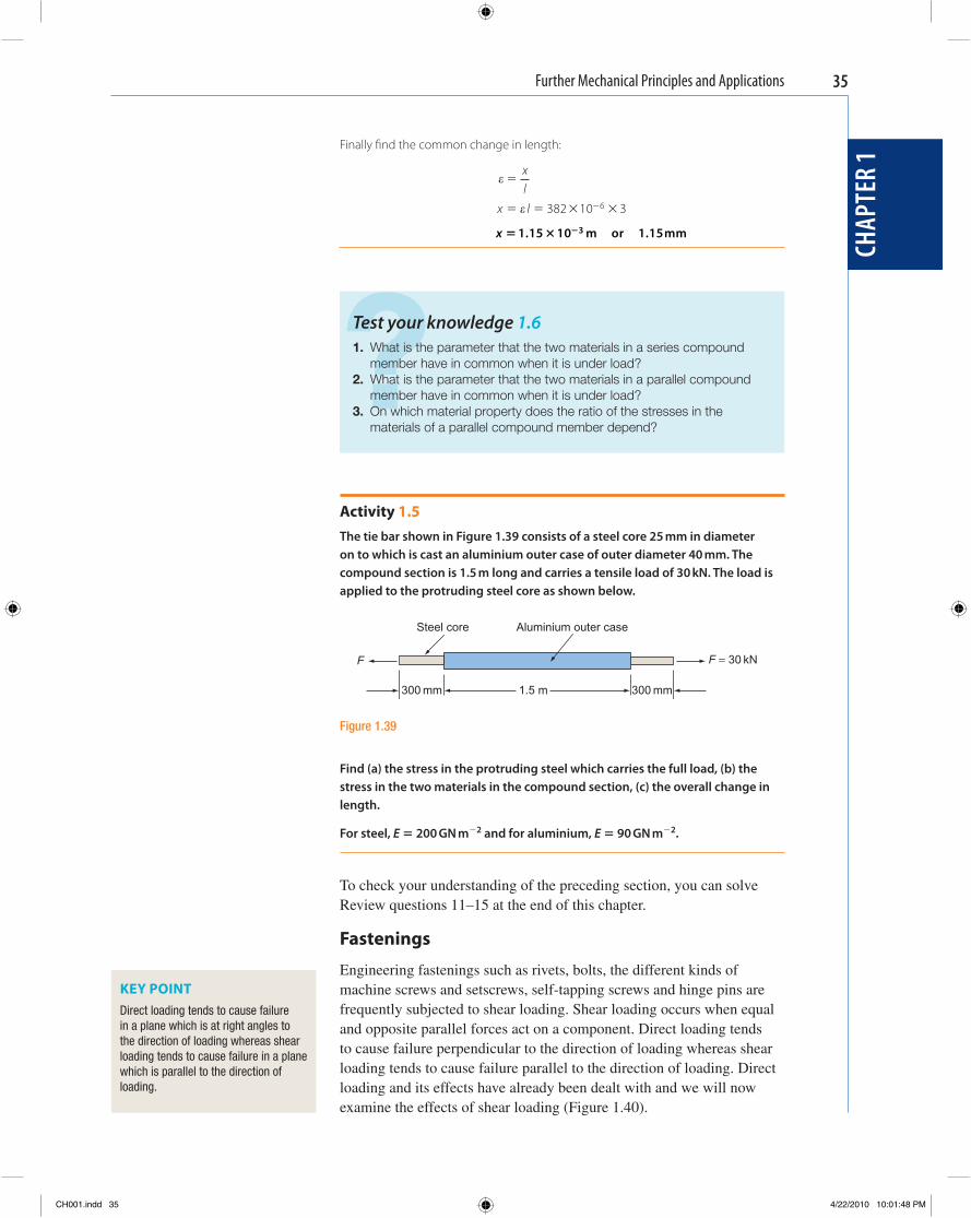
Activity 1.5 The tie bar shown in Figure 1.39 consists of a steel core 25 mm in diameter on to which is cast an aluminium outer case of outer diameter 40 mm. The compound section is 1.5 m long and carries a tensile load of 30 kN. The load is applied to the protruding steel core as shown below.
Steel core Aluminium outer case
F F = 30 kN
300 mm 1.5 m 300 mm
Figure 1.39
Find (a) the stress in the protruding steel which carries the full load, (b) the stress in the two materials in the compound section, (c) the overall change in length.
For steel, E � 200 GN m � 2 and for aluminium, E � 90 GN m � 2 .
To check your understanding of the preceding section, you can solve Review questions 11–15 at the end of this chapter.
Fastenings
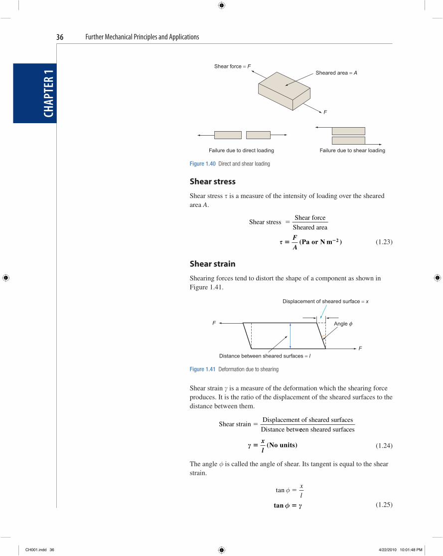
Engineering fastenings such as rivets, bolts, the different kinds of machine screws and setscrews, self-tapping screws and hinge pins are frequently subjected to shear loading. Shear loading occurs when equal and opposite parallel forces act on a component. Direct loading tends to cause failure perpendicular to the direction of loading whereas shear loading tends to cause failure parallel to the direction of loading. Direct loading and its effects have already been dealt with and we will now examine the effects of shear loading ( Figure 1.40 ).
KEY POINT Direct loading tends to cause failure in a plane which is at right angles to the direction of loading whereas shear loading tends to cause failure in a plane which is parallel to the direction of loading.
CH001.indd 35CH001.indd 35 4/22/2010 10:01:48 PM4/22/2010 10:01:48 PM
Further Mechanical Principles and Applications
CHAP
TER
136
Shear stress
Shear stress � is a measure of the intensity of loading over the sheared area A .
Shear stress
Shear force
Sheared area�
� � �F
A( )Pa or N m 2 (1.23)
Shear strain
Shearing forces tend to distort the shape of a component as shown in Figure 1.41 .
Shear force = FSheared area = A
F
Failure due to direct loading Failure due to shear loading
Figure 1.40 Direct and shear loading
Displacement of sheared surface = x
F Angle φ
FDistance between sheared surfaces = l
Figure 1.41 Deformation due to shearing
Shear strain is a measure of the deformation which the shearing force produces. It is the ratio of the displacement of the sheared surfaces to the distance between them.
Shear strain
Displacement of sheared surfaces
Distance betw�
eeen sheared surfaces
� �
xl
( )No units (1.24)
The angle φ is called the angle of shear. Its tangent is equal to the shear strain.
tan φ �
x
l
tan φ � � (1.25)
CH001.indd 36CH001.indd 36 4/22/2010 10:01:48 PM4/22/2010 10:01:48 PM
Further Mechanical Principles and Applications
CHAP
TER
1
37
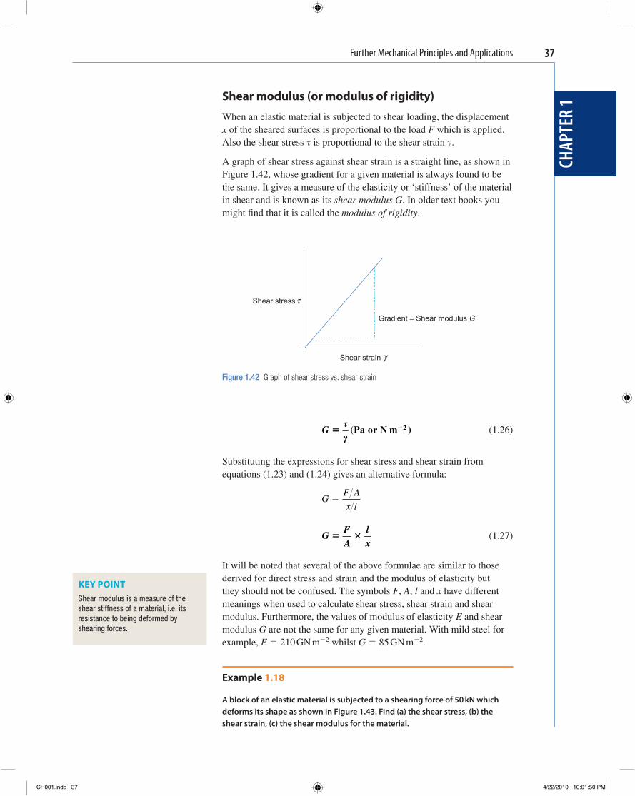
Shear modulus (or modulus of rigidity)
When an elastic material is subjected to shear loading, the displacement x of the sheared surfaces is proportional to the load F which is applied. Also the shear stress � is proportional to the shear strain .
A graph of shear stress against shear strain is a straight line, as shown in Figure 1.42 , whose gradient for a given material is always found to be the same. It gives a measure of the elasticity or ‘ stiffness ’ of the material in shear and is known as its shear modulus G . In older text books you might fi nd that it is called the modulus of rigidity .
τShear stress
Gradient = Shear modulus G
Shear strain γ
Figure 1.42 Graph of shear stress vs. shear strain
G � ��
�( )Pa or N m 2
(1.26)
Substituting the expressions for shear stress and shear strain from equations (1.23) and (1.24) gives an alternative formula:
G
F A
x l�
G
FA
lx
� � (1.27)
It will be noted that several of the above formulae are similar to those derived for direct stress and strain and the modulus of elasticity but they should not be confused. The symbols F , A , l and x have different meanings when used to calculate shear stress, shear strain and shear modulus. Furthermore, the values of modulus of elasticity E and shear modulus G are not the same for any given material. With mild steel for example, E � 210 GN m � 2 whilst G � 85 GN m � 2 .
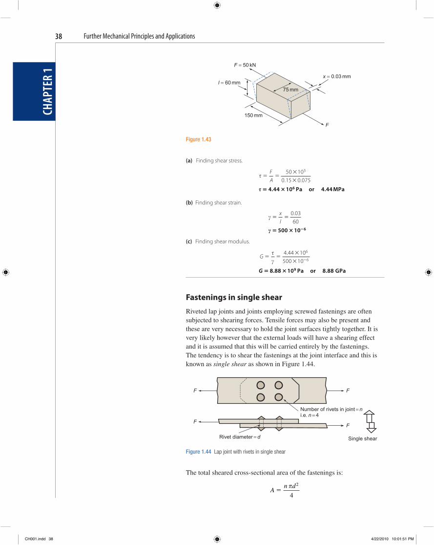
Example 1.18
A block of an elastic material is subjected to a shearing force of 50 kN which deforms its shape as shown in Figure 1.43 . Find (a) the shear stress, (b) the shear strain, (c) the shear modulus for the material.
KEY POINT Shear modulus is a measure of the shear stiffness of a material, i.e. its resistance to being deformed by shearing forces.
CH001.indd 37CH001.indd 37 4/22/2010 10:01:50 PM4/22/2010 10:01:50 PM
Further Mechanical Principles and Applications
CHAP
TER
138
(a) Finding shear stress.
� � �
�
�
FA
50 100 15 0 075
3
. .
� � �4 44 10 4 446. .Pa or MPa
(b) Finding shear strain.
� �
xl
0 0360.
� � � �500 10 6
(c) Finding shear modulus.
G � �
�
� �
�
4 44 10500 10
6
6
.
G � �8 88 10 8 889. .Pa or GPa
Fastenings in single shear
Riveted lap joints and joints employing screwed fastenings are often subjected to shearing forces. Tensile forces may also be present and these are very necessary to hold the joint surfaces tightly together. It is very likely however that the external loads will have a shearing effect and it is assumed that this will be carried entirely by the fastenings. The tendency is to shear the fastenings at the joint interface and this is known as single shear as shown in Figure 1.44 .
F = 50 kN
x = 0.03 mml = 60 mm
150 mm
F
75 mm
Figure 1.43
F F
Number of rivets in joint = ni.e. n = 4
FF
Rivet diameter = d Single shear
Figure 1.44 Lap joint with rivets in single shear
The total sheared cross-sectional area of the fastenings is:
A
n d�
� 2
4
CH001.indd 38CH001.indd 38 4/22/2010 10:01:51 PM4/22/2010 10:01:51 PM
Further Mechanical Principles and Applications
CHAP
TER
1
39
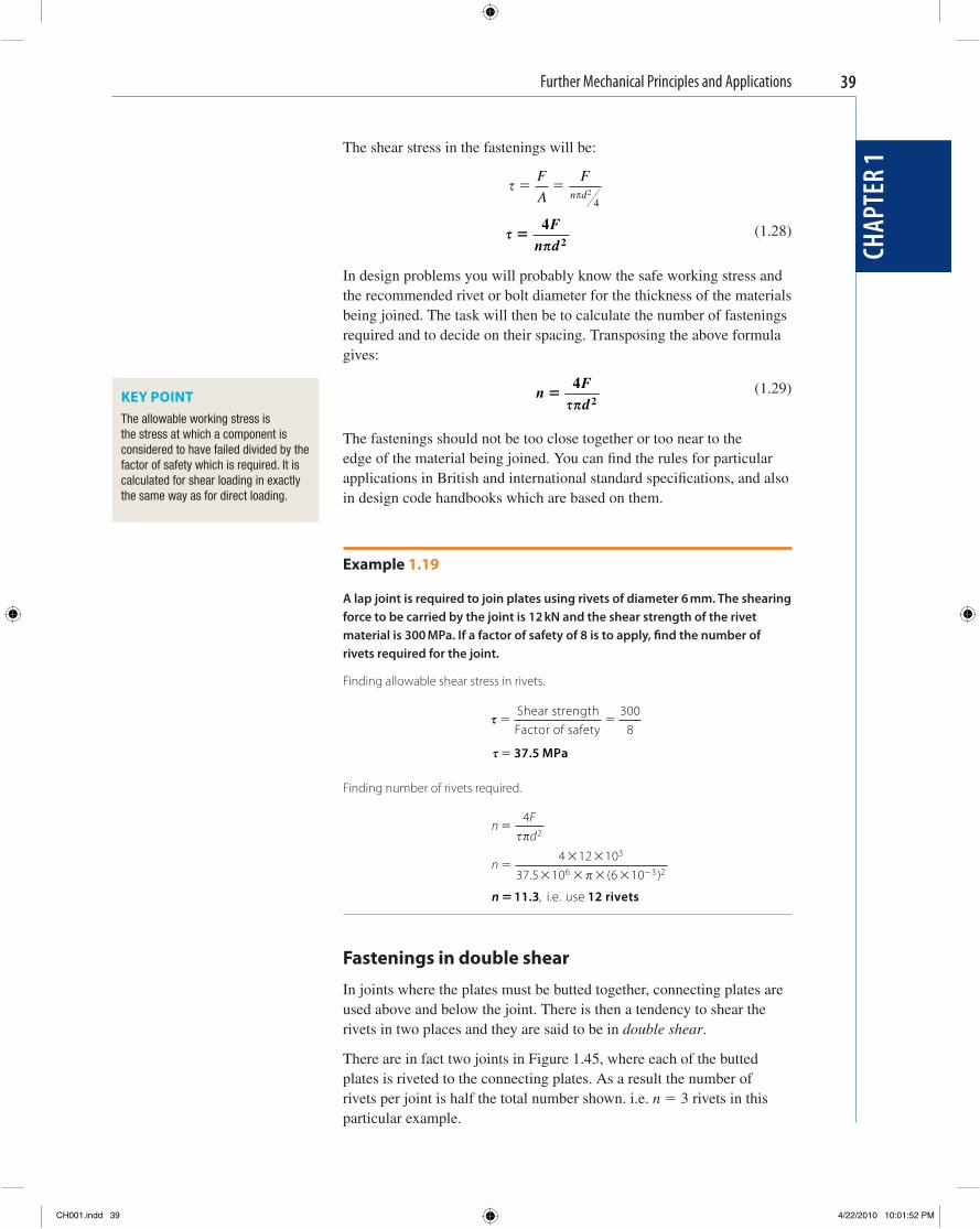
The shear stress in the fastenings will be:
� � �
F
A
Fn d� 2
4
�
��
42
Fn d
(1.28)
In design problems you will probably know the safe working stress and the recommended rivet or bolt diameter for the thickness of the materials being joined. The task will then be to calculate the number of fastenings required and to decide on their spacing. Transposing the above formula gives:
n
Fd
�4
2�� (1.29)
The fastenings should not be too close together or too near to the edge of the material being joined. You can fi nd the rules for particular applications in British and international standard specifi cations, and also in design code handbooks which are based on them.
Example 1.19
A lap joint is required to join plates using rivets of diameter 6 mm. The shearing force to be carried by the joint is 12 kN and the shear strength of the rivet material is 300 MPa. If a factor of safety of 8 is to apply, fi nd the number of rivets required for the joint.
Finding allowable shear stress in rivets.
� � �
Shear strengthFactor of safety
3008
� � 37 5. MPa
Finding number of rivets required.
nFd
n
�
�� �
� � � � �
4
4 12 1037 5 10 6 10
2
3
6 3 2
��
�. ( )
n � 11 3 12. , i.e. use rivets
Fastenings in double shear
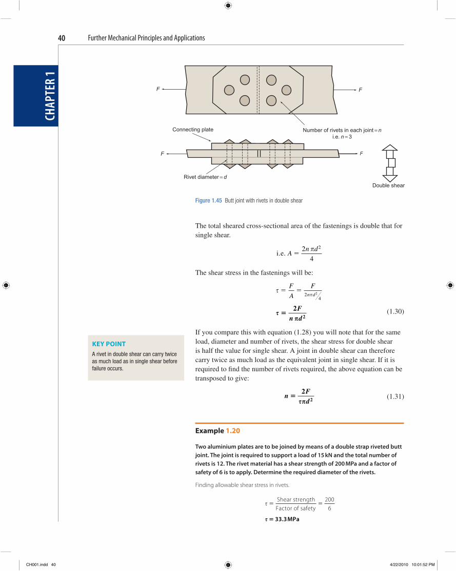
In joints where the plates must be butted together, connecting plates are used above and below the joint. There is then a tendency to shear the rivets in two places and they are said to be in double shear .
There are in fact two joints in Figure 1.45 , where each of the butted plates is riveted to the connecting plates. As a result the number of rivets per joint is half the total number shown. i.e. n � 3 rivets in this particular example.
KEY POINT The allowable working stress is the stress at which a component is considered to have failed divided by the factor of safety which is required. It is calculated for shear loading in exactly the same way as for direct loading.
CH001.indd 39CH001.indd 39 4/22/2010 10:01:52 PM4/22/2010 10:01:52 PM
Further Mechanical Principles and Applications
CHAP
TER
140
The total sheared cross-sectional area of the fastenings is double that for single shear.
i.e. A
n d�
2
4
2�
The shear stress in the fastenings will be:
� � �
F
A
Fn d2
42π
�
��
22
Fn d
(1.30)
If you compare this with equation (1.28) you will note that for the same load, diameter and number of rivets, the shear stress for double shear is half the value for single shear. A joint in double shear can therefore carry twice as much load as the equivalent joint in single shear. If it is required to fi nd the number of rivets required, the above equation can be transposed to give:
n
Fd
�2
2�� (1.31)
Example 1.20
Two aluminium plates are to be joined by means of a double strap riveted butt joint. The joint is required to support a load of 15 kN and the total number of rivets is 12. The rivet material has a shear strength of 200 MPa and a factor of safety of 6 is to apply. Determine the required diameter of the rivets.
Finding allowable shear stress in rivets.
� � �
Shear strengthFactor of safety
2006
� � 33 3. MPa
KEY POINT A rivet in double shear can carry twice as much load as in single shear before failure occurs.
Figure 1.45 Butt joint with rivets in double shear
Connecting plate
FF
FF
Number of rivets in each joint = ni.e. n = 3
Rivet diameter = d
Double shear
CH001.indd 40CH001.indd 40 4/22/2010 10:01:52 PM4/22/2010 10:01:52 PM
Further Mechanical Principles and Applications
CHAP
TER
1
41
Finding required rivet diameter.
��
��
��
�
�
�
� � �
�� �
� �
2
2
2 122
6
2 10 106 3
2
2
3
Fn d
dF
n
dF
nn
d
where rivets
33 3 106. �
d � � �5 64 10 5 646 0
3. ..
m or mm i.e. use mm rivets
,
? Test your knowledge 1.7 1. What is the difference between direct loading and shear loading? 2. Defi ne shear stress and shear strain. 3. What is the angle of shear? 4. Defi ne shear modulus. 5. Compare the load carrying capacity for rivets of a given diameter when
subjected to single shear and double shear.
Activity 1.6 Two steel plates are riveted together by means of a lap joint. Ten rivets of diameter 9 mm are used and the load carried is 20 kN. What is the shear stress in the rivet material and the factor of safety in operation if the shear strength is 300 MPa? If the lap joint were replaced by a double strap butt joint with 10 rivets per joint and each carrying the same shear stress as above, what would be the required rivet diameter?
To check your understanding of the preceding section, you can solve Review questions 16–19 at the end of this chapter.
Rotating Systems with Uniform Angular Acceleration
By uniform angular motion we mean rotation at a steady speed or rotation with uniform angular acceleration or retardation. If you have completed the core unit Mechanical Principles and Applications you will be familiar with uniform linear motion and the equations that connect linear displacement, time, velocity and acceleration. You may also recall the expressions for work power, momentum and energy. We shall now develop a similar set of equations for angular motion.
The symbols that we use for linear and angular parameters are shown in Table 1.2 .
The unit of angular displacement or angle turned is the radian. There are other ways of measuring angles you will be familiar with, such as degrees of arc and number of revolutions turned. However, it is the
CH001.indd 41CH001.indd 41 4/22/2010 10:01:53 PM4/22/2010 10:01:53 PM
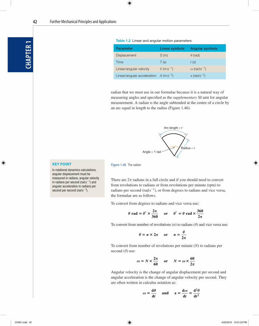
Further Mechanical Principles and Applications
CHAP
TER
142
radian that we must use in our formulae because it is a natural way of measuring angles and specifi ed as the supplementary SI unit for angular measurement. A radian is the angle subtended at the centre of a circle by an arc equal in length to the radius ( Figure 1.46 ).
Table 1.2 Linear and angular motion parameters
Parameter Linear symbols Angular symbols
Displacement S (m) � (rad)
Time T (s) t (s)
Linear/angular velocity V (m s � 1 ) (rad s � 1 )
Linear/angular acceleration A (m s � 2 ) � (rad s � 2 )
Angle = 1 rad
Arc length = r
Radius = r
Figure 1.46 The radian
There are 2 � radians in a full circle and if you should need to convert from revolutions to radians or from revolutions per minute (rpm) to radians per second (rad s � 1 ), or from degrees to radians and vice versa, the formulae are as follows.
To convert from degrees to radians and vice versa use:
� �
�� �
� rad rad� � � �° °2
3603602
or
To convert from number of revolutions ( n ) to radians ( � ) and vice versa use:
� �
�
�� � �n n2
2or
To convert from number of revolutions per minute ( N ) to radians per second ( � ) use:
�
�� � � �N N
260
602
or
Angular velocity is the change of angular displacement per second and angular acceleration is the change of angular velocity per second. They are often written in calculus notation as:
��
�� � �
dd
dd
dd
2
t t tand
2
KEY POINT In rotational dynamics calculations, angular displacement must be measured in radians, angular velocity in radians per second (rad s � 1 ) and angular acceleration in radians per second per second (rad s � 2 ).
CH001.indd 42CH001.indd 42 4/22/2010 10:01:53 PM4/22/2010 10:01:53 PM
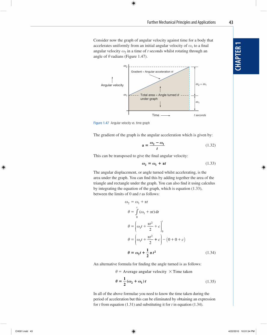
Further Mechanical Principles and Applications
CHAP
TER
1
43
Consider now the graph of angular velocity against time for a body that accelerates uniformly from an initial angular velocity of 1 to a fi nal angular velocity 2 in a time of t seconds whilst rotating through an angle of � radians ( Figure 1.47 ).
Angular velocity
Gradient = Angular acceleration
Time
ω 2 = ω1
ω 1
ω1
ω2
t seconds
Total area = Angle turnedunder graph
θ
α
Figure 1.47 Angular velocity vs. time graph
The gradient of the graph is the angular acceleration which is given by:
�
�
�2 1
t (1.32)
This can be transposed to give the fi nal angular velocity:
�2 1� � t (1.33)
The angular displacement, or angle turned whilst accelerating, is the area under the graph. You can fi nd this by adding together the area of the triangle and rectangle under the graph. You can also fi nd it using calculus by integrating the equation of the graph, which is equation (1.33),between the limits of 0 and t as follows:
�
� �
� �
� �
2 1
10
1
2
0
1
2
2
2
� �
� �
� � �
� �
t
t t
tt
c
tt
t
t
( )∫
⎛
⎝⎜⎜⎜⎜
⎞
⎠⎟⎟⎟⎟
d
�� � � �c c⎛
⎝⎜⎜⎜⎜
⎞
⎠⎟⎟⎟⎟ ( )0 0
� �� �1
212
t t (1.34)
An alternative formula for fi nding the angle turned is as follows:
� � �Average angular velocity Time taken
� � �
12 2 1( ) t
(1.35)
In all of the above formulae you need to know the time taken during the period of acceleration but this can be eliminated by obtaining an expression for t from equation (1.31) and substituting it for t in equation (1.34).
CH001.indd 43CH001.indd 43 4/22/2010 10:01:54 PM4/22/2010 10:01:54 PM
Further Mechanical Principles and Applications
CHAP
TER
144
�
�
��
��
1 2
1 2
t
t
Substituting for t in equation (1.34) gives:
�
���
� ��
� � �
1
2
2
2 11 2
2 1 1 2
( )
( ) ( )
⎛
⎝⎜⎜⎜
⎞
⎠⎟⎟⎟⎟
Rearranging gives:
2
222
2 1 2 1 12
22
12
��
��
� � � �
� �
��22
12 2� � (1.36)
As you will see in Table 1.3 , the equations for linear and angular motion are very similar.
Table 1.3 Equations for uniform linear and angular motion
Linear motion Angular motion
� � u � at 2 � 1 � � t
s � ut � ½ at 2 � � 1 t � ½ � t 2
s � ½ ( u � � ) t � � ½ ( 2 � 1 ) t
� 2 � u 2 � 2 as 2 2 � 1 2 � 2 � �
Here are a few more useful formulae for converting arc length s to angle turned � , tangential linear velocity v to angular velocity and tangential linear acceleration � to angular acceleration � and vice versa.
� �
� �
� � �
� � �
sr
vr
ar
s r v r a ror
Example 1.21
The winding drum of a hoist is 250 mm in diameter and is accelerated uniformly from rest to a speed of 120 rpm in a time of 45 s. Determine (a) the fi nal angular velocity of the drum, (b) the angular acceleration, (c) the number of revolutions turned during the period of acceleration, (d) the height that the load on the hoist is raised, (e) the fi nal velocity of the load.
(a) Finding fi nal angular velocity of drum in rad s � 1 .
� �2 2
260
120260
� � � �N
2112 6� . rad s�
KEY POINT The gradient of a graph of angular velocity against time is the angular acceleration and the area under the graph is the angular displacement.
CH001.indd 44CH001.indd 44 4/22/2010 10:01:54 PM4/22/2010 10:01:54 PM
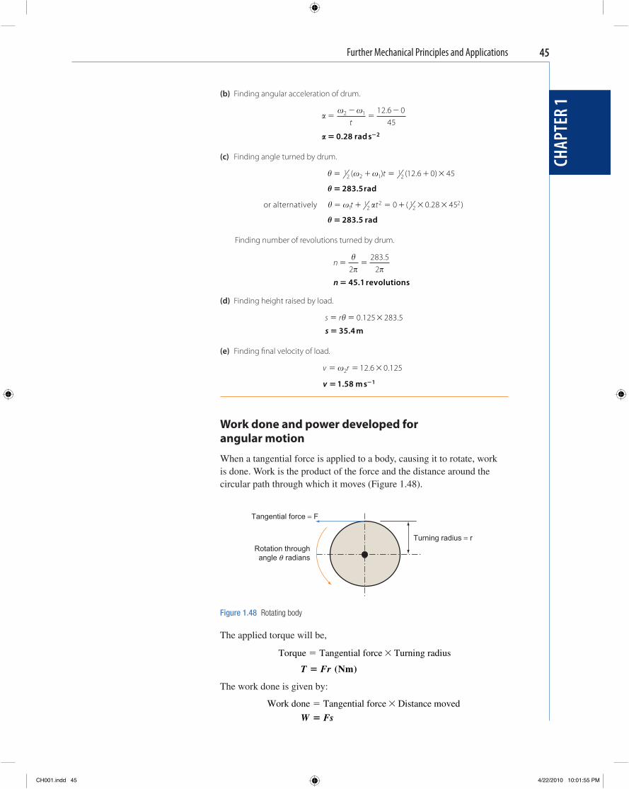
Further Mechanical Principles and Applications
CHAP
TER
1
45
(b) Finding angular acceleration of drum.
�
�
��
�2 1 12 6 045t.
� � �0 28 2. rad s
(c) Finding angle turned by drum.
� � � � � �12 2 1
12 12 6 0 45( ) ( . )t
� � 283 5. rad
or alternatively � �� � � � � �11
22 1
220 0 28 45t t ( . )
� � 283 5. rad
Finding number of revolutions turned by drum.
n � �
�� �2
283 52
.
n � 45 1. revolutions
(d) Finding height raised by load.
s r� � �� 0 125 283 5. .
s � 35 4. m
(e) Finding fi nal velocity of load.
v r� � �2 12 6 0 125. .
v � �1 58 1. m s
Work done and power developed for angular motion
When a tangential force is applied to a body, causing it to rotate, work is done. Work is the product of the force and the distance around the circular path through which it moves ( Figure 1.48 ).
Tangential force = F
Turning radius = rRotation throughangle radiansθ
Figure 1.48 Rotating body
The applied torque will be,
Torque Tangential force Turning radius� �
T Fr� ( )Nm The work done is given by:
Work done Tangential force Distance moved� �
W Fs�
CH001.indd 45CH001.indd 45 4/22/2010 10:01:55 PM4/22/2010 10:01:55 PM
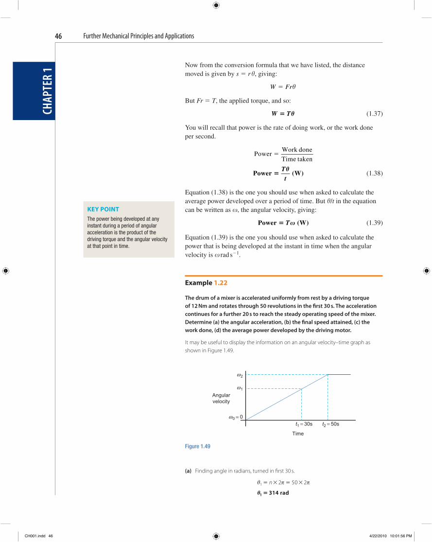
Further Mechanical Principles and Applications
CHAP
TER
146
Now from the conversion formula that we have listed, the distance moved is given by s � r � , giving:
W Fr� �
But Fr � T , the applied torque, and so:
W T� � (1.37)
You will recall that power is the rate of doing work, or the work done per second.
Power
Work done
Time taken�
Power W�
Tt�
( ) (1.38)
Equation (1.38) is the one you should use when asked to calculate the average power developed over a period of time. But � / t in the equation can be written as , the angular velocity, giving:
Power W� T ( ) (1.39)
Equation (1.39) is the one you should use when asked to calculate the power that is being developed at the instant in time when the angular velocity is rad s � 1 .
Example 1.22
The drum of a mixer is accelerated uniformly from rest by a driving torque of 12 Nm and rotates through 50 revolutions in the fi rst 30 s. The acceleration continues for a further 20 s to reach the steady operating speed of the mixer. Determine (a) the angular acceleration, (b) the fi nal speed attained, (c) the work done, (d) the average power developed by the driving motor.
It may be useful to display the information on an angular velocity–time graph as shown in Figure 1.49 .
KEY POINT The power being developed at any instant during a period of angular acceleration is the product of the driving torque and the angular velocity at that point in time.
Angularvelocity
Time
t1 = 30s t2 = 50s
ω2
ω1
ω0 = 0
Figure 1.49
(a) Finding angle in radians, turned in fi rst 30 s.
� � �1 2 50 2� � � �n
�1 314 rad�
CH001.indd 46CH001.indd 46 4/22/2010 10:01:56 PM4/22/2010 10:01:56 PM
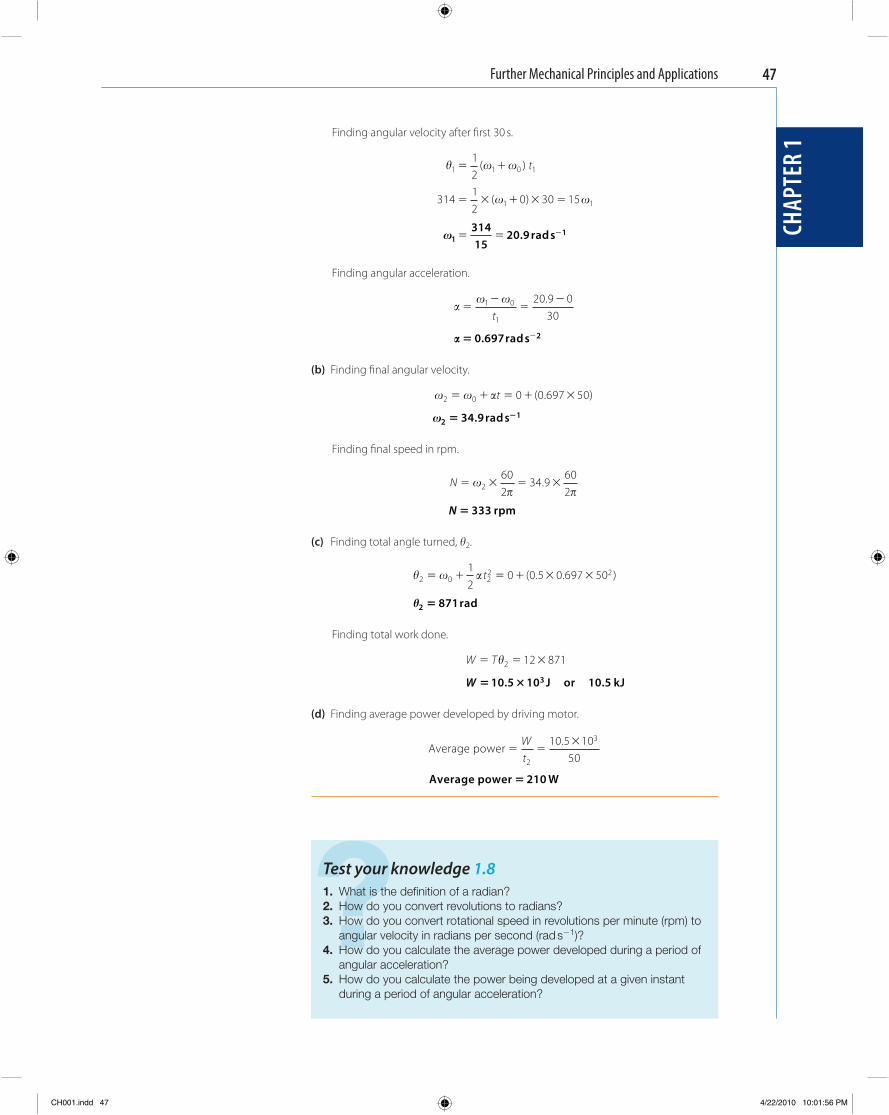
Further Mechanical Principles and Applications
CHAP
TER
1
47
Finding angular velocity after fi rst 30 s.
�
1 1 0 1
1 1
12
31412
0 30 15
� �
� � � � �
( )
( )
t
1
131415
20 9� � �. rad s
Finding angular acceleration.
�
�
��
�1 0
1
20 9 030t.
� � 0 697 2. rad s�
(b) Finding fi nal angular velocity.
�2 0 0 0 697 50� � � � �t ( . )
2134 9� �. rad s
Finding fi nal speed in rpm.
N � � � �
� �2602
34 9602
.
N � 333 rpm
(c) Finding total angle turned, � 2 .
� �2 0 2
2 212
0 0 5 0 697 50� � � � � �t ( . . )
�2 871� rad
Finding total work done.
W T� � ��2 12 871
W � �10 5 10 10 53. or .J kJ
(d) Finding average power developed by driving motor.
Average power � �
�Wt2
310 5 1050
.
Average power W� 210
? Test your knowledge 1.8 1. What is the defi nition of a radian? 2. How do you convert revolutions to radians? 3. How do you convert rotational speed in revolutions per minute (rpm) to
angular velocity in radians per second (rad s � 1 )? 4. How do you calculate the average power developed during a period of
angular acceleration? 5. How do you calculate the power being developed at a given instant
during a period of angular acceleration?
CH001.indd 47CH001.indd 47 4/22/2010 10:01:56 PM4/22/2010 10:01:56 PM
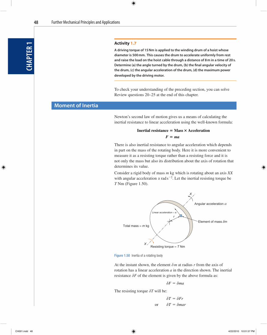
Further Mechanical Principles and Applications
CHAP
TER
148
Activity 1.7 A driving torque of 15 Nm is applied to the winding drum of a hoist whose diameter is 500 mm. This causes the drum to accelerate uniformly from rest and raise the load on the hoist cable through a distance of 8 m in a time of 20 s. Determine (a) the angle turned by the drum, (b) the fi nal angular velocity of the drum, (c) the angular acceleration of the drum, (d) the maximum power developed by the driving motor.
To check your understanding of the preceding section, you can solve Review questions 20–25 at the end of this chapter.
Moment of Inertia
Newton ’ s second law of motion gives us a means of calculating the inertial resistance to linear acceleration using the well-known formula:
Inertial resistance Mass Acceleration� �
�F ma
There is also inertial resistance to angular acceleration which depends in part on the mass of the rotating body. Here it is more convenient to measure it as a resisting torque rather than a resisting force and it is not only the mass but also its distribution about the axis of rotation that determines its value.
Consider a rigid body of mass m kg which is rotating about an axis XX with angular acceleration � rad s � 2 . Let the inertial resisting torque be T Nm ( Figure 1.50 ).
X
r
Element of mass m
Angular acceleration α
Linear acceleration = a
Total mass = m kg
Resisting torque = T Nm
X
δ
Figure 1.50 Inertia of a rotating body
At the instant shown, the element � m at radius r from the axis of rotation has a linear acceleration a in the direction shown. The inertial resistance � F of the element is given by the above formula as:
� �F ma�
The resisting torque � T will be:
� �T Fr�
or � �T mar�
CH001.indd 48CH001.indd 48 4/22/2010 10:01:57 PM4/22/2010 10:01:57 PM
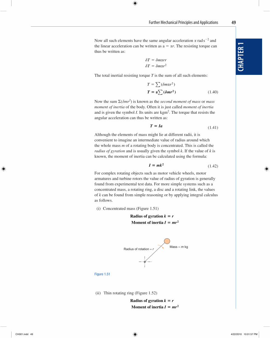
Further Mechanical Principles and Applications
CHAP
TER
1
49
Now all such elements have the same angular acceleration � rad s � 2 and the linear acceleration can be written as a � � r . The resisting torque can thus be written as:
� � �T m rr�
� � �T m r� 2
The total inertial resisting torque T is the sum of all such elements:
T m r� ( )� � 2∑
T mr� � ( )2∑
(1.40)
Now the sum � ( � mr 2 ) is known as the second moment of mass or mass moment of inertia of the body. Often it is just called moment of inertia and is given the symbol I . Its units are kgm 2 . The torque that resists the angular acceleration can thus be written as:
T Ia� (1.41)
Although the elements of mass might lie at different radii, it is convenient to imagine an intermediate value of radius around which the whole mass m of a rotating body is concentrated. This is called the radius of gyration and is usually given the symbol k . If the value of k is known, the moment of inertia can be calculated using the formula:
I mk� 2 (1.42)
For complex rotating objects such as motor vehicle wheels, motor armatures and turbine rotors the value of radius of gyration is generally found from experimental test data. For more simple systems such as a concentrated mass, a rotating ring, a disc and a rotating link, the values of k can be found from simple reasoning or by applying integral calculus as follows.
(i) Concentrated mass ( Figure 1.51 )
Radius of gyration
Moment of inertia
k r
I mr
�
� 2
Radius of rotation = r Mass = m kg
Figure 1.51
(ii) Thin rotating ring ( Figure 1.52 )
Radius of gyration
Moment of inertia
k r
I mr
�
� 2
CH001.indd 49CH001.indd 49 4/22/2010 10:01:57 PM4/22/2010 10:01:57 PM
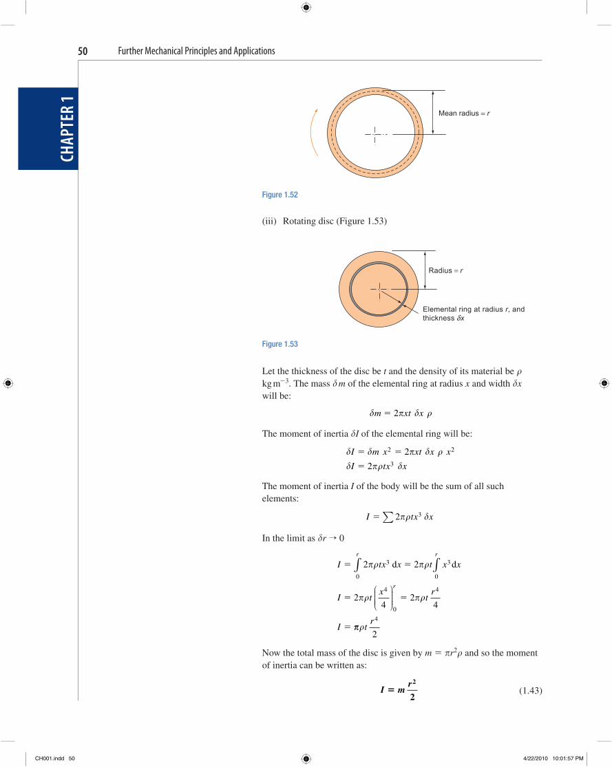
Further Mechanical Principles and Applications
CHAP
TER
150
(iii) Rotating disc ( Figure 1.53 )
Radius = r
Elemental ring at radius r, andthickness xδ
Figure 1.53
Mean radius = r
Figure 1.52
Let the thickness of the disc be t and the density of its material be kg m � 3 . The mass � m of the elemental ring at radius x and width � x will be:
� � � m xt x� 2
The moment of inertia � I of the elemental ring will be:
� � � �
� � �
I m x xt x x
I tx x
� �
�
2 2
3
2
2
The moment of inertia I of the body will be the sum of all such elements:
I tx x� 2 3� �∑
In the limit as � r → 0
I tx x t x x
I tx
tr
I
r r
r
� �
� �
�
2 2
24
24
3
0
3
0
4
0
4
� �
� �
d d∫ ∫
⎛
⎝⎜⎜⎜⎜
⎞
⎠⎟⎟⎟⎟
�� tr4
2
Now the total mass of the disc is given by m � � r 2 and so the moment of inertia can be written as:
I m
r�
2
2 (1.43)
CH001.indd 50CH001.indd 50 4/22/2010 10:01:57 PM4/22/2010 10:01:57 PM

Further Mechanical Principles and Applications
CHAP
TER
1
51
Because I � mk 2 , the radius of gyration k of a disc is given by:
k
r22
2�
k
rr� �
20 7071.
(1.44)
You may also have encountered this fi gure of 0.7071 in your electrical principles studies where it gives the root-mean square value of an alternating current when multiplied by the peak value. This is very much the same idea, since the radius of gyration is the square root of the sum of all the squared values of the elemental radii.
(iv) Rod rotating about a perpendicular axis through its centre ( Figure 1.54 )
xδx
l/2 l/2
Figure 1.54
Let a be the mass per unit length of the rod. The mass � m of the element of length � x distance x from the central axis will be:
� �m a x�
The moment of inertia � I of the element will be:
� � �
� �
I mx a xx
I ax x
� �
�
2 2
2
The total moment of inertia is the sum of all such elements:
I ax x
I a x x
�
�
2
2
�
�
∑∑
In the limit as � x → 0
I a x x
I ax
asl l
l
l
l
l
�
� �
2
2
2
3
2
2 3 3
3 24 24
d�
�
�
�
�
∫
⎛
⎝⎜⎜⎜⎜
⎞
⎠⎟⎟⎟⎟
⎛
⎝⎜⎜⎜⎜
⎞
⎠⎟⎟⎟⎟⎟
I al
�3
12
Now the mass m of the rod is given by m � al and so the moment of inertia of the rod can be written as:
I m
l�
2
12 (1.45)
CH001.indd 51CH001.indd 51 4/22/2010 10:01:58 PM4/22/2010 10:01:58 PM
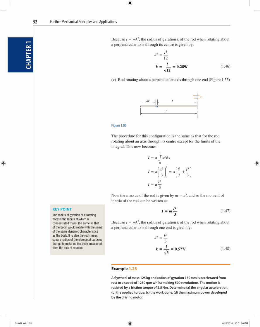
Further Mechanical Principles and Applications
CHAP
TER
152
Because I � mk 2 , the radius of gyration k of the rod when rotating about a perpendicular axis through its centre is given by:
k
l22
12�
k
ll� �
120 289.
(1.46)
(v) Rod rotating about a perpendicular axis through one end ( Figure 1.55 )
l
xδx
Figure 1.55
The procedure for this confi guration is the same as that for the rod rotating about an axis through its centre except for the limits of the integral. This now becomes:
I a x x
I ax
al l
I al
�
� �
�
2
0
1
3
0
1 3 3
3
3 3 3
3
d∫
⎛
⎝⎜⎜⎜⎜
⎞
⎠⎟⎟⎟⎟
⎛
⎝⎜⎜⎜⎜
⎞
⎠⎟⎟⎟⎟�
Now the mass m of the rod is given by m � al , and so the moment of inertia of the rod can be written as:
I m
l�
2
3 (1.47)
Because I � mk 2 , the radius of gyration k of the rod when rotating about a perpendicular axis through one end is given by:
k
l22
3�
k
ll� �
30 577.
(1.48)
Example 1.23
A fl ywheel of mass 125 kg and radius of gyration 150 mm is accelerated from rest to a speed of 1250 rpm whilst making 500 revolutions. The motion is resisted by a friction torque of 2.5 Nm. Determine (a) the angular acceleration, (b) the applied torque, (c) the work done, (d) the maximum power developed by the driving motor.
KEY POINT The radius of gyration of a rotating body is the radius at which a concentrated mass, the same as that of the body, would rotate with the same of the same dynamic characteristics as the body. It is also the root-mean square radius of the elemental particles that go to make up the body, measured from the axis of rotation.
CH001.indd 52CH001.indd 52 4/22/2010 10:01:58 PM4/22/2010 10:01:58 PM
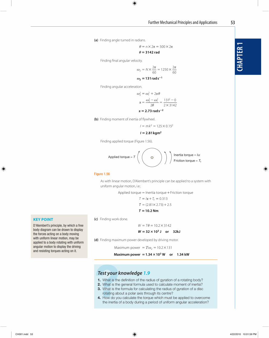
Further Mechanical Principles and Applications
CHAP
TER
1
53
(a) Finding angle turned in radians.
� � �� � � �n 2 500 2
� � 3142 rad
Finding fi nal angular velocity.
� �2
260
1250260
� � � �N
21131� �rad s
Finding angular acceleration.
��
�
�
22
12
22
12 2
2
2131 02 3142
�
��
��
�
�
� � �2 73 2. rad s
(b) Finding moment of inertia of fl ywheel.
I m k� � �2 2125 0 15.
I � 2 81 2. kgm
Finding applied torque ( Figure 1.56 ).
Applied torque = TInertia torque = Iα
Friction torque = Tf
Figure 1.56
As with linear motion, D ’ Alembert ’ s principle can be applied to a system with uniform angular motion, i.e.:
Applied torque Inertia torque Friction torque
f
� �
� � �T I T� 0 313.
TT � � �( . . ) .2 81 2 73 2 5
T � 10 2. Nm
(c) Finding work done.
W T� � �� 10 2 3142.
W � �32 10 323 J kJor
(d) Finding maximum power developed by driving motor.
Maximum power � � �Τ2 10 2 131.
Maximum power W kW� �1 34 10 1 343. or .
KEY POINT D ’ Alembert ’ s principle, by which a free body diagram can be drawn to display the forces acting on a body moving with uniform linear motion, may be applied to a body rotating with uniform angular motion to display the driving and resisting torques acting on it.
? Test your knowledge 1.9 1. What is the defi nition of the radius of gyration of a rotating body? 2. What is the general formula used to calculate moment of inertia? 3. What is the formula for calculating the radius of gyration of a disc
rotating about a polar axis through its centre? 4. How do you calculate the torque which must be applied to overcome
the inertia of a body during a period of uniform angular acceleration?
CH001.indd 53CH001.indd 53 4/22/2010 10:01:59 PM4/22/2010 10:01:59 PM
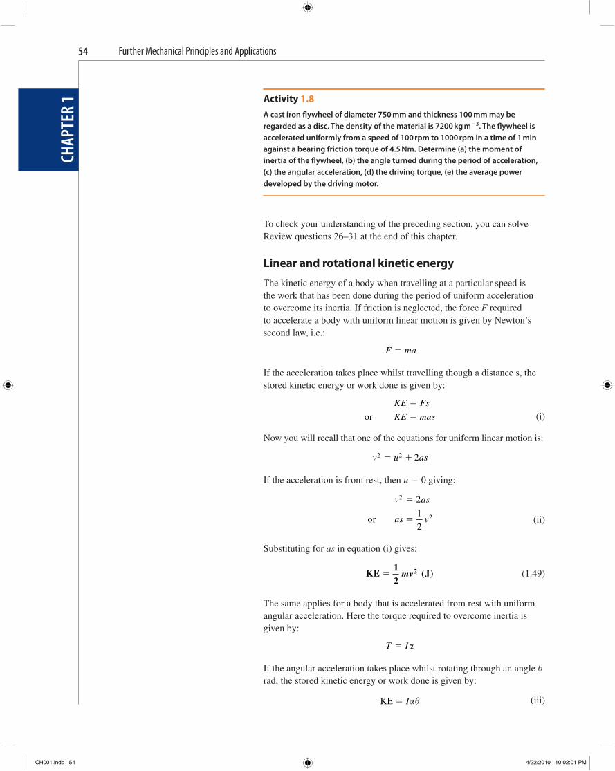
Further Mechanical Principles and Applications
CHAP
TER
154
Activity 1.8 A cast iron fl ywheel of diameter 750 mm and thickness 100 mm may be regarded as a disc. The density of the material is 7200 kg m � 3 . The fl ywheel is accelerated uniformly from a speed of 100 rpm to 1000 rpm in a time of 1 min against a bearing friction torque of 4.5 Nm. Determine (a) the moment of inertia of the fl ywheel, (b) the angle turned during the period of acceleration, (c) the angular acceleration, (d) the driving torque, (e) the average power developed by the driving motor.
To check your understanding of the preceding section, you can solve Review questions 26–31 at the end of this chapter.
Linear and rotational kinetic energy
The kinetic energy of a body when travelling at a particular speed is the work that has been done during the period of uniform acceleration to overcome its inertia. If friction is neglected, the force F required to accelerate a body with uniform linear motion is given by Newton ’ s second law, i.e.:
F ma�
If the acceleration takes place whilst travelling though a distance s, the stored kinetic energy or work done is given by:
KE Fs
KE mas
�
�or (i)
Now you will recall that one of the equations for uniform linear motion is:
v u as2 2 2� �
If the acceleration is from rest, then u � 0 giving:
v as
as v
2
2
2
1
2
�
�or
(ii)
Substituting for as in equation (i) gives:
KE J�
12
2mv ( )
(1.49)
The same applies for a body that is accelerated from rest with uniform angular acceleration. Here the torque required to overcome inertia is given by:
T I� �
If the angular acceleration takes place whilst rotating through an angle � rad, the stored kinetic energy or work done is given by:
KE � I�� (iii)
CH001.indd 54CH001.indd 54 4/22/2010 10:02:01 PM4/22/2010 10:02:01 PM
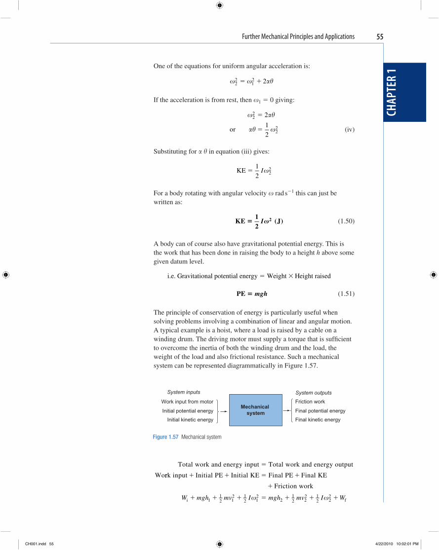
Further Mechanical Principles and Applications
CHAP
TER
1
55
One of the equations for uniform angular acceleration is:
��22
12 2� �
If the acceleration is from rest, then 1 � 0 giving:
��
��
22
22
2
1
2
�
�or
(iv)
Substituting for � � in equation (iii) gives:
KE �
1
2 22I
For a body rotating with angular velocity rad s � 1 this can just be written as:
KE J�
12
2I ( )
(1.50)
A body can of course also have gravitational potential energy. This is the work that has been done in raising the body to a height h above some given datum level.
i.e. Gravitational potential energy Weight Height raised� �
PE � mgh (1.51)
The principle of conservation of energy is particularly useful when solving problems involving a combination of linear and angular motion. A typical example is a hoist, where a load is raised by a cable on a winding drum. The driving motor must supply a torque that is suffi cient to overcome the inertia of both the winding drum and the load, the weight of the load and also frictional resistance. Such a mechanical system can be represented diagrammatically in Figure 1.57 .
System inputs System outputs
Work input from motor Friction work
Initial potential energy Final potential energy
Initial kinetic energy Final kinetic energy
Mechanical system
Figure 1.57 Mechanical system
Total work and energy input Total work and energy output
Wo
�
rrk input Initial PE Initial KE Final PE Final KE
Friction
� � � �
� work
i 112 1
2 12 2
12 2
2 12 fW mgh mv I mgh mv I W� � � � � � � 1
222
CH001.indd 55CH001.indd 55 4/22/2010 10:02:01 PM4/22/2010 10:02:01 PM
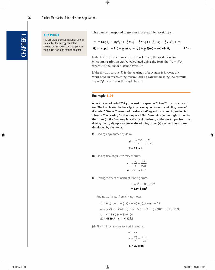
Further Mechanical Principles and Applications
CHAP
TER
156
This can be transposed to give an expression for work input.
W mgh mgh mv mv I I Wi f� � � � � � �( ) ( ) ( )2 112 2
2 12 1
2 12 2
2 12 1
2
W mg h h m v v I Wi f� � � � � � �( ) ( ) ( )2 112 2
212 1
2 22
12 (1.52)
If the frictional resistance force F f is known, the work done in overcoming friction can be calculated using the formula, W f � F f s , where s is the linear distance travelled.
If the friction torque T f in the bearings of a system is known, the work done in overcoming friction can be calculated using the formula W f � T f � , where � is the angle turned.
Example 1.24
A hoist raises a load of 75 kg from rest to a speed of 2.5 m s � 1 in a distance of 6 m. The load is attached to a light cable wrapped around a winding drum of diameter 500 mm. The mass of the drum is 60 kg and its radius of gyration is 180 mm. The bearing friction torque is 5 Nm. Determine (a) the angle turned by the drum, (b) the fi nal angular velocity of the drum, (c) the work input from the driving motor, (d) input torque to the winding drum, (e) the maximum power developed by the motor.
(a) Finding angle turned by drum.
� �
��
h hr
2 1 60 25.
� � 24 rad
(b) Finding fi nal angular velocity of drum.
2
2 2 50 25
� �vr
..
2110� �rad s
(c) Finding moment of inertia of winding drum.
I Mk� � �2 260 0 18.
I � 1 94 2. kgm
Finding work input from driving motor.
W mg h h m v v T
W
i12
12 f
i1
� � � � � � �
� � � �
( ) ( ) ( )
[ . ] [
2 1 22
12
22
12
75 9 81 6
�
2212
i
� � � � � � � �
� � � �
75 2 5 0 10 0 5 24
4415 234 50 120
2 2( . )] [ ( )] [ ]
W
Wi J kJ� 4819 4 82or .
(d) Finding input torque from driving motor.
W T
TW
i i
ii
�
� �
�
�4819
24
Ti Nm� 201
KEY POINT The principle of conservation of energy states that the energy cannot be created or destroyed but changes may take place from one form to another.
CH001.indd 56CH001.indd 56 4/22/2010 10:02:01 PM4/22/2010 10:02:01 PM
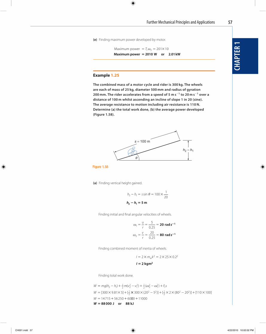
Further Mechanical Principles and Applications
CHAP
TER
1
57
(e) Finding maximum power developed by motor.
Maximum power i� � �T 2 201 10 Maximum power W kW� 2010 2 01or .
Example 1.25
The combined mass of a motor cycle and rider is 300 kg. The wheels are each of mass of 25 kg, diameter 500 mm and radius of gyration 200 mm. The rider accelerates from a speed of 5 m s � 1 to 20 m s � 1 over a distance of 100 m whilst ascending an incline of slope 1 in 20 (sine). The average resistance to motion including air resistance is 110 N. Determine (a) the total work done, (b) the average power developed ( Figure 1.58 ).
s = 100 m
θ
h2 – h1
Figure 1.58
(a) Finding vertical height gained.
h h s2 1 100
120
� � � �sin �
h h2 1 5� � m
Finding initial and fi nal angular velocities of wheels.
1
2
50 2520
0 25
� � �
� � �
urvr
.
.
20 rad
80 rad
1
1
s
s
�
�
Finding combined moment of inertia of wheels.
I m k� � � � �2 2 25 0 22 2w .
I � 2 2kgm
Finding total work done.
W mg h h m v v F s
W
� � � � � � �
� � � �
( ) ( ) ( )
[ . ] [
2 1 22
12
22
12
300 9 81 5
12
12 f
12
�� � � � � � � � �
� � �
300 20 5 2 80 20 110 100
14715 56 250 60
2 2 2 2( )] [ ( )] [ ]12
W 000 11000�
W � 88 000 J 88 kJor
CH001.indd 57CH001.indd 57 4/22/2010 10:02:02 PM4/22/2010 10:02:02 PM
Further Mechanical Principles and Applications
CHAP
TER
158
Activity 1.9 A mine cage of mass 3 tonnes is accelerated uniformly upwards from a speed of 1.0 m s � 1 to 4.5 m s � 1 in a time of 20 s. The winding drum which is 1.5 m in diameter has a mass of 1 tonne and has the dynamic characteristics of a disc. The average frictional resistance in the cage guides is 500 N and there is a bearing friction torque of 45 Nm. The mass of the lift cable can be neglected. Determine (a) the angle turned by the winding drum, (b) the moment of inertia of the winding drum, (c) the total work done, (d) the input torque to the winding drum, (e) the maximum power developed by the driving motor.
To check your understanding of the preceding section, you can solve Review questions 32–35 at the end of this chapter.
Experiments to determine moment of inertia and radius of gyration
There are a number of experimental methods which may be used to determine the moment of inertia and radius of gyration of a rotating body. Two methods, which are within the scope of this chapter, will be described. The fi rst method may be applied to bodies which rotate on an axle which is supported in bearings. The second method makes use of an inclined plane or track.
Method 1 ApparatusRotating body under investigation which is mounted on an axle. The axle may be supported in bearings or between free-running centres at some distance above ground level as shown in Figure 1.59 . Length of cord, hanger and slotted masses, metre rule, stopwatch.
? Test your knowledge 1.10 1. What is gravitational potential energy? 2. What is kinetic energy? 3. What is the principle of conservation of energy? 4. How can you calculate the work done in overcoming a friction torque? 5. Write down the energy equation for a mechanical system?
(b) Finding time taken.
s v u t
ts
v u
� �
��
��
�
12 ( )
( ) ( )2 2 100
20 5
t � 8 s
Finding average power developed.
Average power � �
Wt
88 0008
Average power W kW� 11000 11or
CH001.indd 58CH001.indd 58 4/22/2010 10:02:02 PM4/22/2010 10:02:02 PM

Further Mechanical Principles and Applications
CHAP
TER
1
59
Rotating mass = M kg Radius of axle = r
Falling mass = m kg
h
Figure 1.59 Arrangement of apparatus
Procedure 1. Measure the diameter of the axle and record the value of its radius r . 2. Wind the cord around the axle and attach the hanger to its free end. 3. Place small slotted masses on the hanger until bearing friction is
just overcome. The hanger and masses should then fall with a slow uniform velocity.
4. Rewind the cord and place an additional mass of m kg on the hanger. 5. Measure and record the distance h from the base of the hanger to the
ground. 6. Release the hanger and record the time for it to fall to the ground.
Repeat this operation a number of times and obtain the average time of fall.
7. Calculate the moment of inertia and radius of gyration of the rotating body using the following derived formulae.
Theory Finding fi nal velocity of falling mass.
h v v t� �
1
2 2 1( )
But v 1 � 0,
h v t�
1
2 2
v
ht2
2�
(i)
Finding fi nal angular velocity of rotating body.
2
2�v
r
2
2�
hrt
(ii)
CH001.indd 59CH001.indd 59 4/22/2010 10:02:03 PM4/22/2010 10:02:03 PM
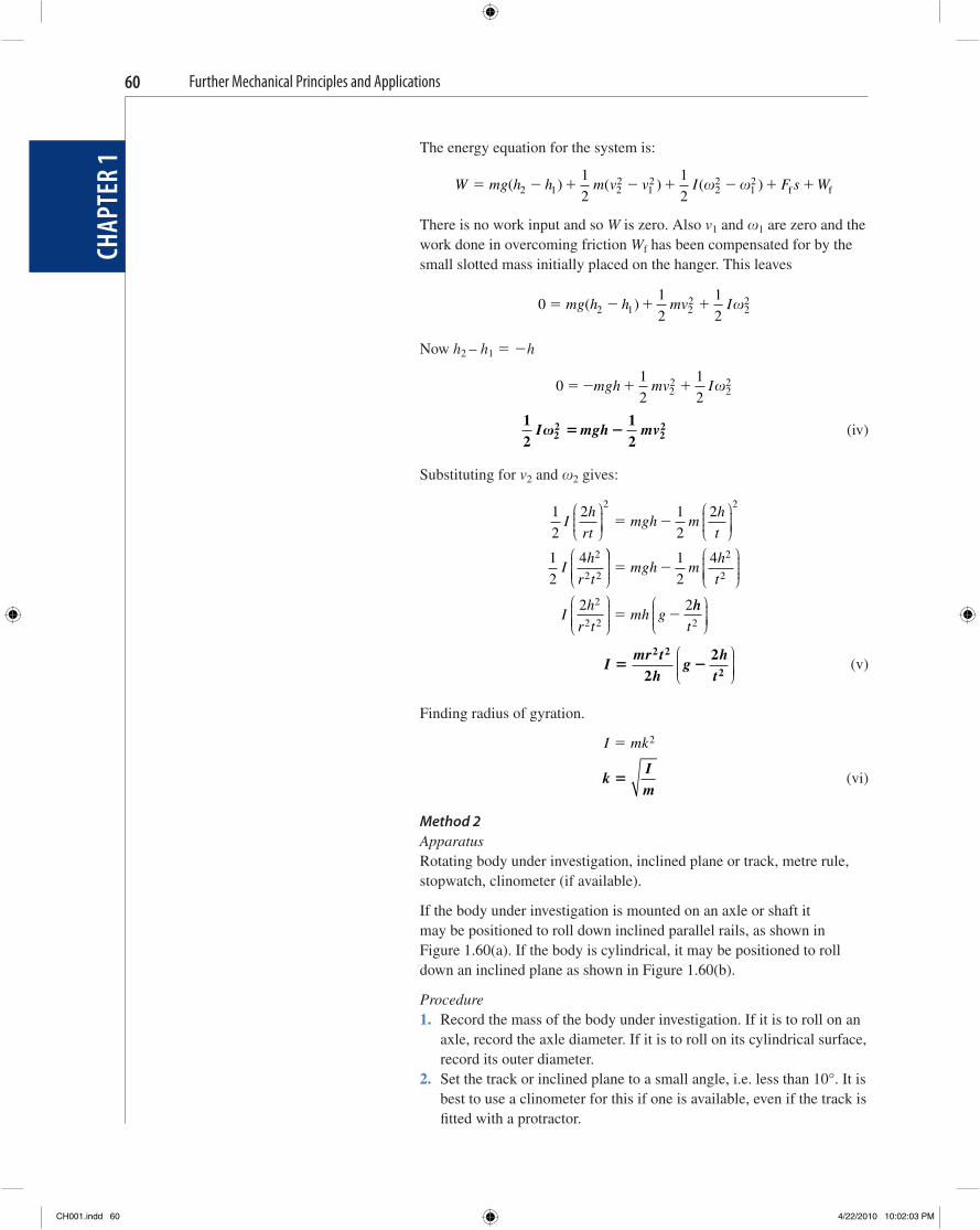
Further Mechanical Principles and Applications
CHAP
TER
160
The energy equation for the system is:
W mg h h m v v I F s W� � � � � � � �( ) ( ) ( )2 1 2
212
22
121
2
1
2 f f
There is no work input and so W is zero. Also v 1 and 1 are zero and the work done in overcoming friction W f has been compensated for by the small slotted mass initially placed on the hanger. This leaves
0
1
2
1
22 1 22
22� � � �mg h h mv I( )
Now h 2 – h 1 � � h
0
1
2
1
222
22� � � �mgh mv I
12
122
222I mgh mv � �
(iv)
Substituting for v 2 and 2 gives:
1
2
2 1
2
2
1
2
4
2 2
2
2 2
Ih
rtmgh m
h
t
Ih
r t
⎛
⎝⎜⎜⎜
⎞
⎠⎟⎟⎟⎟
⎛
⎝⎜⎜⎜
⎞
⎠⎟⎟⎟⎟
⎛
⎝⎜⎜⎜⎜
� �
⎞⎞
⎠⎟⎟⎟⎟
⎛
⎝⎜⎜⎜⎜
⎞
⎠⎟⎟⎟⎟
⎛
⎝⎜⎜⎜⎜
⎞
⎠⎟⎟⎟⎟
� �
� �
mgh mh
t
Ih
r tmh g
1
2
4
2 2
2
2
2
2 2
hh
t2
⎛
⎝⎜⎜⎜
⎞
⎠⎟⎟⎟⎟
I
mr th
gh
t� �
2 2
222⎛
⎝⎜⎜⎜
⎞
⎠⎟⎟⎟⎟
(v)
Finding radius of gyration.
I mk� 2
k
Im
�
(vi)
Method 2 Apparatus Rotating body under investigation, inclined plane or track, metre rule, stopwatch, clinometer (if available).
If the body under investigation is mounted on an axle or shaft it may be positioned to roll down inclined parallel rails, as shown in Figure 1.60(a) . If the body is cylindrical, it may be positioned to roll down an inclined plane as shown in Figure 1.60(b) .
Procedure 1. Record the mass of the body under investigation. If it is to roll on an
axle, record the axle diameter. If it is to roll on its cylindrical surface, record its outer diameter.
2. Set the track or inclined plane to a small angle, i.e. less than 10 ° . It is best to use a clinometer for this if one is available, even if the track is fi tted with a protractor.
CH001.indd 60CH001.indd 60 4/22/2010 10:02:03 PM4/22/2010 10:02:03 PM
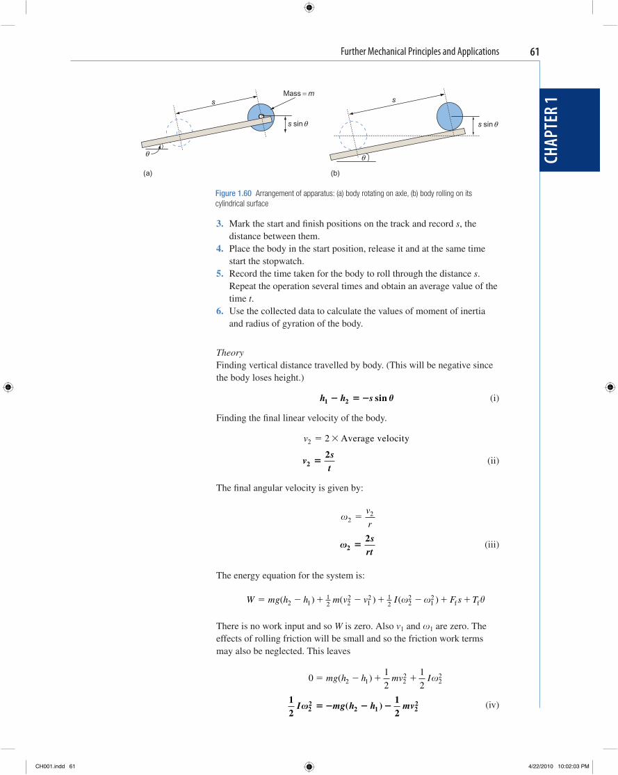
Further Mechanical Principles and Applications
CHAP
TER
1
61
θ θ
ssMass = m
(a) (b)
s sinθ s sinθ
Figure 1.60 Arrangement of apparatus: (a) body rotating on axle, (b) body rolling on its cylindrical surface
3. Mark the start and fi nish positions on the track and record s , the distance between them.
4. Place the body in the start position, release it and at the same time start the stopwatch.
5. Record the time taken for the body to roll through the distance s . Repeat the operation several times and obtain an average value of the time t .
6. Use the collected data to calculate the values of moment of inertia and radius of gyration of the body.
Theory Finding vertical distance travelled by body. (This will be negative since the body loses height.)
h h s1 2� � � sin � (i)
Finding the fi nal linear velocity of the body.
v2 2� � Average velocity
v
st2
2�
(ii)
The fi nal angular velocity is given by:
2
2�v
r
2
2�
srt
(iii)
The energy equation for the system is:
W mg h h m v v I F s T� � � � � � � �( ) ( ) ( )2 1 22
12
22
121
212 f f �
There is no work input and so W is zero. Also v 1 and 1 are zero. The effects of rolling friction will be small and so the friction work terms may also be neglected. This leaves
0
1
2
1
22 1 22
22� � � �mg h h mv I( )
12
122
22 1 2
2I mg h h mv � � � �( )
(iv)
CH001.indd 61CH001.indd 61 4/22/2010 10:02:03 PM4/22/2010 10:02:03 PM
Further Mechanical Principles and Applications
CHAP
TER
162
Substituting for h 1 – h 2 and v 2 and 2 gives:
1
2
2 1
2
2
1
2
4
2 2
2
2
Is
rtmg s m
s
t
Is
r
⎛
⎝⎜⎜⎜
⎞
⎠⎟⎟⎟⎟
⎛
⎝⎜⎜⎜
⎞
⎠⎟⎟⎟⎟� � � �( )sin �
ttmgs m
s
t
Is
r t
2
2
2
2
2 2
1
2
4
2
⎛
⎝⎜⎜⎜⎜
⎞
⎠⎟⎟⎟⎟
⎛
⎝⎜⎜⎜⎜
⎞
⎠⎟⎟⎟⎟
⎛
⎝⎜⎜⎜⎜
� �sin �
⎞⎞
⎠⎟⎟⎟⎟
⎛
⎝⎜⎜⎜
⎞
⎠⎟⎟⎟⎟
⎛
⎝⎜⎜⎜
⎞
� �
� �
ms gs
t
Imsr t
sg
s
t
sin
sin
�
�
2
2
2
2
2 2
2 2 ⎠⎠⎟⎟⎟⎟
I
mr ts
gs
t� �
2 2
222
sin �⎛
⎝⎜⎜⎜
⎞
⎠⎟⎟⎟⎟
(v)
Finding radius of gyration.
I mk� 2
k
Im
�
(vi)
Note : The expressions for moment of inertia may also be obtained by applying D ’ Alembert ’ s principle and Newton ’ s second law of motion to the systems.
Centripetal Acceleration and Centripetal Force
Newton ’ s fi rst law of motion states that a moving body will continue in a straight line unless acted upon by some external force . It follows that when a body is travelling in a circular path, there must be some sideways force pushing, or pulling it, towards the centre of rotation. This is known as centripetal force, which means ‘ centre seeking ’ . With a car travelling round a curve, the centripetal force is provided by friction between the tyres and the road surface and with an orbiting satellite, it is provided by the earth ’ s gravitational pull.
Vector change of velocity
You will recall that velocity is a vector quantity. This means that it has both magnitude and direction. For a body travelling in a straight path we very often only state the magnitude of its velocity, i.e. its speed. We take its direction for granted but strictly speaking, we should state both magnitude and direction when we write down the velocity of a body.
Because velocity is a vector quantity, it can be represented in magnitude, direction and sense by a line v 1 drawn to a suitable scale on a vector diagram. If either the speed or direction of a body should change, then its velocity will change. The new vector v 2 will be drawn from the same starting point but to a different length or in a different direction. There
KEY POINT Velocity is a vector quantity and if either the speed or the direction of a body changes, its velocity will change.
CH001.indd 62CH001.indd 62 4/22/2010 10:02:04 PM4/22/2010 10:02:04 PM
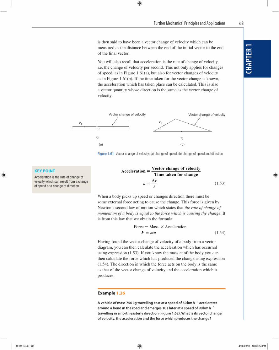
Further Mechanical Principles and Applications
CHAP
TER
1
63
AccelerationVector change of velocity
Time taken for chang�
ee
av
t�
�
(1.53)
When a body picks up speed or changes direction there must be some external force acting to cause the change. This force is given by Newton ’ s second law of motion which states that the rate of change of momentum of a body is equal to the force which is causing the change . It is from this law that we obtain the formula:
Force Mass Acceleration� �
F ma� (1.54)
Having found the vector change of velocity of a body from a vector diagram, you can then calculate the acceleration which has occurred using expression (1.53). If you know the mass m of the body you can then calculate the force which has produced the change using expression (1.54). The direction in which the force acts on the body is the same as that of the vector change of velocity and the acceleration which it produces.
Example 1.26
A vehicle of mass 750 kg travelling east at a speed of 50 km h � 1 accelerates around a bend in the road and emerges 10 s later at a speed of 90 km h � 1 travelling in a north easterly direction ( Figure 1.62 ). What is its vector change of velocity, the acceleration and the force which produces the change?
is then said to have been a vector change of velocity which can be measured as the distance between the end of the initial vector to the end of the fi nal vector.
You will also recall that acceleration is the rate of change of velocity, i.e. the change of velocity per second. This not only applies for changes of speed, as in Figure 1.61(a) , but also for vector changes of velocity as in Figure 1.61(b) . If the time taken for the vector change is known, the acceleration which has taken place can be calculated. This is also a vector quantity whose direction is the same as the vector change of velocity.
(a) (b)
v2 v2
v1v1
Vector change of velocity Vector change of velocity
Figure 1.61 Vector change of velocity: (a) change of speed, (b) change of speed and direction
KEY POINT Acceleration is the rate of change of velocity which can result from a change of speed or a change of direction.
CH001.indd 63CH001.indd 63 4/22/2010 10:02:04 PM4/22/2010 10:02:04 PM
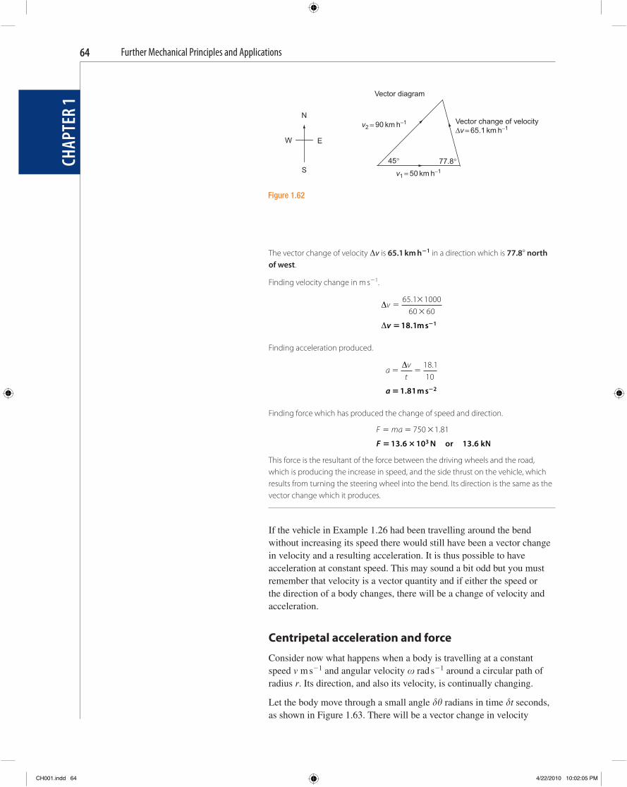
Further Mechanical Principles and Applications
CHAP
TER
164
The vector change of velocity � v is 65.1 km h � 1 in a direction which is 77.8 � north of west .
Finding velocity change in m s � 1 .
�v �
�
�
65 1 100060 60.
�v � �18 1 1. m s
Finding acceleration produced.
a
vt
� �� 18 1
10.
a � �1 81 2. m s
Finding force which has produced the change of speed and direction.
F ma� � �750 1 81.
F � �13 6 10 13 63. or .N kN This force is the resultant of the force between the driving wheels and the road, which is producing the increase in speed, and the side thrust on the vehicle, which results from turning the steering wheel into the bend. Its direction is the same as the vector change which it produces.
If the vehicle in Example 1.26 had been travelling around the bend without increasing its speed there would still have been a vector change in velocity and a resulting acceleration. It is thus possible to have acceleration at constant speed. This may sound a bit odd but you must remember that velocity is a vector quantity and if either the speed or the direction of a body changes, there will be a change of velocity and acceleration.
Centripetal acceleration and force
Consider now what happens when a body is travelling at a constant speed v m s � 1 and angular velocity rad s � 1 around a circular path of radius r . Its direction, and also its velocity, is continually changing.
Let the body move through a small angle � � radians in time � t seconds, as shown in Figure 1.63 . There will be a vector change in velocity
Vector change of velocityΔv = 65.1 km h−1
45° 77.8°
v2 = 90 km h−1
v1 = 50 km h−1
N
E
S
W
Vector diagram
Figure 1.62
CH001.indd 64CH001.indd 64 4/22/2010 10:02:05 PM4/22/2010 10:02:05 PM
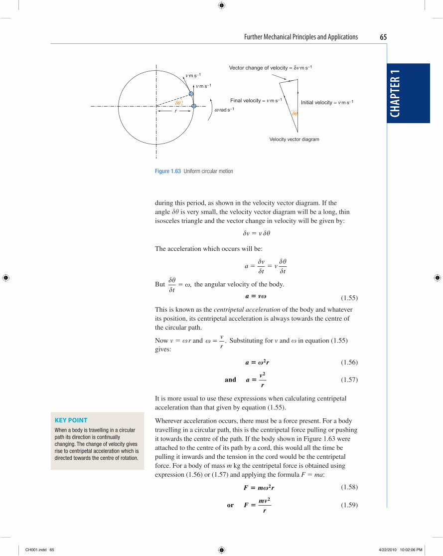
Further Mechanical Principles and Applications
CHAP
TER
1
65
during this period, as shown in the velocity vector diagram. If the angle � � is very small, the velocity vector diagram will be a long, thin isosceles triangle and the vector change in velocity will be given by:
� ��v v�
The acceleration which occurs will be:
a
v
tv
t� �
��
���
But ���
t
� , the angular velocity of the body.
a v� (1.55)
This is known as the centripetal acceleration of the body and whatever its position, its centripetal acceleration is always towards the centre of the circular path.
Now v � r and �v
r. Substituting for v and in equation (1.55)
gives:
a r� 2 (1.56)
and a
vr
�2
(1.57)
It is more usual to use these expressions when calculating centripetal acceleration than that given by equation (1.55).
Wherever acceleration occurs, there must be a force present. For a body travelling in a circular path, this is the centripetal force pulling or pushing it towards the centre of the path. If the body shown in Figure 1.63 were attached to the centre of its path by a cord, this would all the time be pulling it inwards and the tension in the cord would be the centripetal force. For a body of mass m kg the centripetal force is obtained using expression (1.56) or (1.57) and applying the formula F � ma :
F m r� 2 (1.58)
or F
mvr
�2
(1.59)
δθ
δθr
Velocity vector diagram
rad s−1ωFinal velocity = Initial velocity =
Vector change of velocity =m s−1ν
m s−1ν m s−1ν
m s−1ν δ
m s−1ν
Figure 1.63 Uniform circular motion
KEY POINT When a body is travelling in a circular path its direction is continually changing. The change of velocity gives rise to centripetal acceleration which is directed towards the centre of rotation.
CH001.indd 65CH001.indd 65 4/22/2010 10:02:06 PM4/22/2010 10:02:06 PM
Further Mechanical Principles and Applications
CHAP
TER
166
Example 1.27
A body of mass 5 kg travels in a horizontal circular path of radius 2 m at a speed of 100 rpm and is attached to the centre of rotation by a steel rod of diameter 3 mm. Determine (a) the centripetal acceleration of the mass, (b) the centripetal force, (c) the tensile stress in the rod.
(a) Finding angular velocity of rotation.
� �� � � �N ( )rpm
260
100260
� �10 5 1. rad s
Finding centripetal acceleration of mass.
a r� � �2 210 5 2.
a � �219 2m s
(b) Finding centripetal force.
F ma� � �5 219
F � �1 10 10 1 103. or .N kN
(c) Finding cross-sectional area of rod.
A
d� �
�� �2 2
40 0034.
A � � �7 07 10 6 2. m
Finding tensile stress in rod.
� � �
�
� �
FA
1 10 107 07 10
3
6
..
� � �155 10 1556 Pa kPaor
? Test your knowledge 1.11 1. What is a vector quantity? 2. How is it possible for a body to have acceleration whilst travelling at
constant speed? 3. In what direction does centripetal force act? 4. What is centrifugal reaction?
KEY POINT Centripetal force is an active force which pulls or pushes a body towards the centre of rotation. Centrifugal force is the equal and opposite reaction whose direction is away from the centre of rotation.
Activity 1.10 A body of mass 0.6 kg rotates on the end of a helical spring of stiff ness 1.2 kN m � 1 in a horizontal plane. The initial distance from the centre of rotation to the centre of the mass is 200 mm. What will be the radius of rotation of the mass and the stretch in the spring when the rotational speed is 300 rpm.
CH001.indd 66CH001.indd 66 4/22/2010 10:02:06 PM4/22/2010 10:02:06 PM

Further Mechanical Principles and Applications
CHAP
TER
1
67
Centrifugal clutches
Centrifugal clutches are to be found on motor-driven equipment such as lawn mowers, mixers and pumps. They engage automatically when the motor speed reaches a predetermined level and do not depend on the skill of the operator.
In its simplest form a centrifugal clutch consists of a drive shaft to which are attached two or more spring loaded masses. These are lined with a friction material on their outer surfaces and rotate inside a drum which is fi xed to the output shaft (see Figure 1.64 ).
Spring of stiffness S N m−1
Input shaft
Output shaft
D/2
r0
Initial clearance = x
Mass m kg
Drum
Figure 1.64 Centrifugal clutch
The masses, or ‘ bobs ’ , are free to slide outwards in guides which are rigidly fi xed to the input shaft. These are not shown in the above diagram. As the angular velocity of the input shaft increases, the masses slide outwards and eventually make contact with the drum. A further increase in speed causes the drive to be transmitted to the output shaft through friction between the masses and the drum.
Let initial clearance between the masses and the drum be x . Let the initial radius of rotation from the centre of the shafts to the
centre of gravity of the masses be r 0 . Let the diameter of the drum be D . Let the coeffi cient of friction between the drum and the masses be � . Let the angular velocity at which the masses just make contact with
the drum be 0 .
When the masses just make contact with the drum, the tension F 0 in the springs is given by:
Spring tension Spring stiffness Extension� �
F Sx0 � (1.60)
This is also the centripetal force acting on the masses whose radius of rotation is now r 0 � x . Equating spring tension and centripetal force
CH001.indd 67CH001.indd 67 4/22/2010 10:02:07 PM4/22/2010 10:02:07 PM
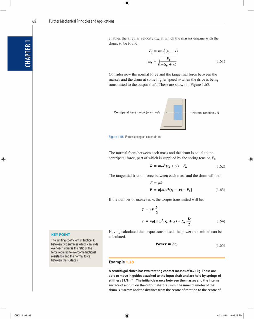
Further Mechanical Principles and Applications
CHAP
TER
168
enables the angular velocity 0 , at which the masses engage with the drum, to be found.
F m r x0 02
0� � ( )
0
0��
F
m r x( )0 (1.61)
Consider now the normal force and the tangential force between the masses and the drum at some higher speed when the drive is being transmitted to the output shaft. These are shown in Figure 1.65 .
KEY POINT The limiting coeffi cient of friction, k , between two surfaces which can slide over each other is the ratio of the force required to overcome frictional resistance and the normal force between the surfaces.
Normal reaction = RCentripetal force = m 2 (r0 + x) − F0ω
Figure 1.65 Forces acting on clutch drum
The normal force between each mass and the drum is equal to the centripetal force, part of which is supplied by the spring tension F 0 .
R m r x F� � �20 0( ) (1.62)
The tangential friction force between each mass and the drum will be:
F R� �
F m r x F� � �� [ ( ) ]20 0 (1.63)
If the number of masses is n , the torque transmitted will be:
T nF
D�
2
T n m r x F
D� � �� [ ( ) ]2
0 0 2 (1.64)
Having calculated the torque transmitted, the power transmitted can be calculated.
Power � T (1.65)
Example 1.28
A centrifugal clutch has two rotating contact masses of 0.25 kg. These are able to move in guides attached to the input shaft and are held by springs of stiff ness 8 kN m � 1 . The initial clearance between the masses and the internal surface of a drum on the output shaft is 5 mm. The inner diameter of the drum is 300 mm and the distance from the centre of rotation to the centre of
CH001.indd 68CH001.indd 68 4/22/2010 10:02:08 PM4/22/2010 10:02:08 PM
Further Mechanical Principles and Applications
CHAP
TER
1
69
gravity of the masses is 135 mm. The coeffi cient of friction between the masses and the drum is 0.35. Determine (a) the rotational speed in revolutions per minute at which the clutch begins to transmit power, (b) the torque and power transmitted at a speed of 1000 rpm.
(a) Finding tension in springs as masses make contact with drum.
F Sx03 38 10 5 10� � � � � �
F0 40� N
Finding angular velocity at which masses just make contact with the drum.
00
0
01
400 25 0 135 0 005
33 8
��
��
� �
Fm r x( ) . ( . . )
. rads
Change to revolutions per minute.
N0 0
602
33 8602
� � � �� �
.
N0 323� rpm
(b) Finding angular velocity at rotational speed of 1000 rpm.
� �� � � �N
260
1000260
� �105 1rad s
Finding torque transmitted at this speed.
T n m r x FD
T
� � �
� � � � � � �
� [ ( ) ]
. [ . ( . . )]
20 0
2
2
2 0 35 0 25 105 0 135 0 005 40⎡⎣⎣⎢
⎤⎦⎥ � 0 15.
T � 36 3. Nm
Finding power transmitted at this speed.
Power � � �T 36 3 105.
Power W kW� �3 81 10 3 813. or .
? Test your knowledge 1.12 1. What are the units in which spring stiffness is measured? 2. If the normal force between two surfaces is 100 N and their coeffi cient
of friction is 0.3, what force will be required to make them slide over each other?
3. What determines the rotational speed at which a centrifugal clutch starts to engage?
4. How do you convert rotational speed in revolutions per minute to angular velocity measured in radians per second?
CH001.indd 69CH001.indd 69 4/22/2010 10:02:08 PM4/22/2010 10:02:08 PM
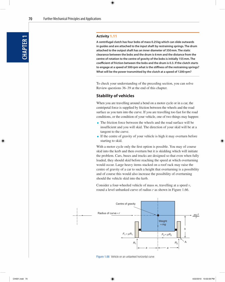
Further Mechanical Principles and Applications
CHAP
TER
170
Weight = mg
m 2r
h
F1 = R1
R2R1
a a
A
Radius of curve = r
Centre of gravity
μ F2 = R2μ
ν
Figure 1.66 Vehicle on an unbanked horizontal curve
Activity 1.11 A centrifugal clutch has four bobs of mass 0.25 kg which can slide outwards in guides and are attached to the input shaft by restraining springs. The drum attached to the output shaft has an inner diameter of 350 mm. The static clearance between the bobs and the drum is 6 mm and the distance from the centre of rotation to the centre of gravity of the bobs is initially 155 mm. The coeffi cient of friction between the bobs and the drum is 0.3. If the clutch starts to engage at a speed of 500 rpm what is the stiff ness of the restraining springs? What will be the power transmitted by the clutch at a speed of 1200 rpm?
To check your understanding of the preceding section, you can solve Review questions 36–39 at the end of this chapter.
Stability of vehicles
When you are travelling around a bend on a motor cycle or in a car, the centripetal force is supplied by friction between the wheels and the road surface as you turn into the curve. If you are travelling too fast for the road conditions, or the condition of your vehicle, one of two things may happen:
● The friction force between the wheels and the road surface will be insuffi cient and you will skid. The direction of your skid will be at a tangent to the curve.
● If the centre of gravity of your vehicle is high it may overturn before starting to skid.
With a motor cycle only the fi rst option is possible. You may of course skid into the kerb and then overturn but it is skidding which will initiate the problem. Cars, buses and trucks are designed so that even when fully loaded, they should skid before reaching the speed at which overturning would occur. Large heavy items stacked on a roof rack may raise the centre of gravity of a car to such a height that overturning is a possibility and of course this would also increase the possibility of overturning should the vehicle skid into the kerb.
Consider a four-wheeled vehicle of mass m , travelling at a speed v , round a level unbanked curve of radius r as shown in Figure 1.66 .
CH001.indd 70CH001.indd 70 4/22/2010 10:02:09 PM4/22/2010 10:02:09 PM
Further Mechanical Principles and Applications
CHAP
TER
1
71
Although the vehicle is moving, it can be considered to be in a state of dynamic equilibrium. In the vertical direction, the active force is the weight W acting downwards which is balanced by the upward reactions R 1 and R 2 of the wheels. The active forces in the horizontal direction are the friction forces F 1 and F 2 which provide the centripetal force. The equal and opposite reaction to them is the centrifugal force given by mv 2 / r . As has been explained, this method of displaying the forces on a free body for a moving object is known as D ’ Alembert ’ s principle.
Let the height of the centre of gravity be h . Let the track width be 2 a . Let the limiting coeffi cient of friction between the wheels and the
road be � .
To fi nd the speed that skidding is likely to occur, equate horizontal forces as the vehicle is about to skid.
Centripetal force Centrifugal reaction�
� �F Fmv
r1 2
2
In the limit as the vehicle is about to skid, F 1 � � R 1 and F 2 � � R 2 . Substituting for these gives:
� �
�
R Rmv
r
R Rmv
r
1 2
2
1 2
2
� �
� �( )
But R 1 � R 2 � mg , the weight of the vehicle.
�
�
mgmv
rrg v
�
�
2
2
v rg� �
(1.66)
To fi nd the speed at which overturning is likely to occur equate moments about the point A in the limit as the vehicle is about to overturn. In this condition R 1 is zero as the nearside wheels are about to lift off the road and all of the weight will be carried on the offside wheels.
Clockwise overturning moment Anticlockwise righting moment�
mmv
rh mga
vgar
h
2
2
�
=
v
ah
rg�
(1.67)
Whichever of the equations (1.66) and (1.67) gives the lower value velocity, that will be the limiting value. You should note that both
KEY POINT When a motor vehicle is travelling round a curve, centripetal force is provided by friction between its tyres and the road surface. When skidding occurs, the vehicle continues in a straight line at a tangent to the curve.
CH001.indd 71CH001.indd 71 4/22/2010 10:02:09 PM4/22/2010 10:02:09 PM
Further Mechanical Principles and Applications
CHAP
TER
172
values of limiting velocity are independent of the mass of the vehicle. Comparing the two equations shows that:
If , the vehicle will skid before the overturning speed��a
h is reached.
If , the vehicle will overturn before th�� a
hee skidding speed is reached.
The reaction of the outer wheels will always be greater than that of the inner wheels. To fi nd these reactions at any speed below that at which overturning is likely take moments about the point A, but this time include the moment of the reaction R 1 .
Clockwise overturning moments Anticlockwise righting momen� tt
mv
rh R a mga
R a mgamv
rh m ga
v h
r
2
1
1
2 2
2
2
� �
� � � �⎛
⎝⎜⎜⎜⎜
⎞
⎠⎟⎟⎟⎟
R
ma
gavr
h1
2
2� �
⎛
⎝⎜⎜⎜⎜
⎞
⎠⎟⎟⎟⎟
(1.68)
Now equate vertical forces to fi nd the reaction of the outer wheels.
R R mg1 2� �
R mg R2 1� � (1.69)
Example 1.29
A car of mass 900 kg travels round an unbanked horizontal curve of radius 30 m. The track width of the car is 1.5 m and its centre of gravity is central and at a height of 0.9 m above the road surface. The limiting coeffi cient of friction between the tyres and the road is 0.7. Show that the car is likely to skid rather than overturn if the speed is excessive and calculate the maximum speed in km h � 1 at which it can travel round the curve. Determine also the reactions of the inner and outer wheels at this speed.
Finding the ratio of half the track width to height of centre of gravity:
ah
� �0 750 9
0 833..
.
Comparing this with the coeffi cient of friction whose value is � � 0.7 shows that:
� <
ah
This indicates that the car will skid before the overturning speed is reached.
Finding speed at which car can travel round the curve, i.e. when skidding is likely to occur.
v rg� � � �� 0 7 30 9 81. .
v � �14 35 1. m s
KEY POINT Properly loaded motor vehicles will skid rather than overturn if their speed around a curve is excessive. Overloading a roof rack can raise the centre of gravity to such a degree that overturning becomes a danger.
CH001.indd 72CH001.indd 72 4/22/2010 10:02:09 PM4/22/2010 10:02:09 PM
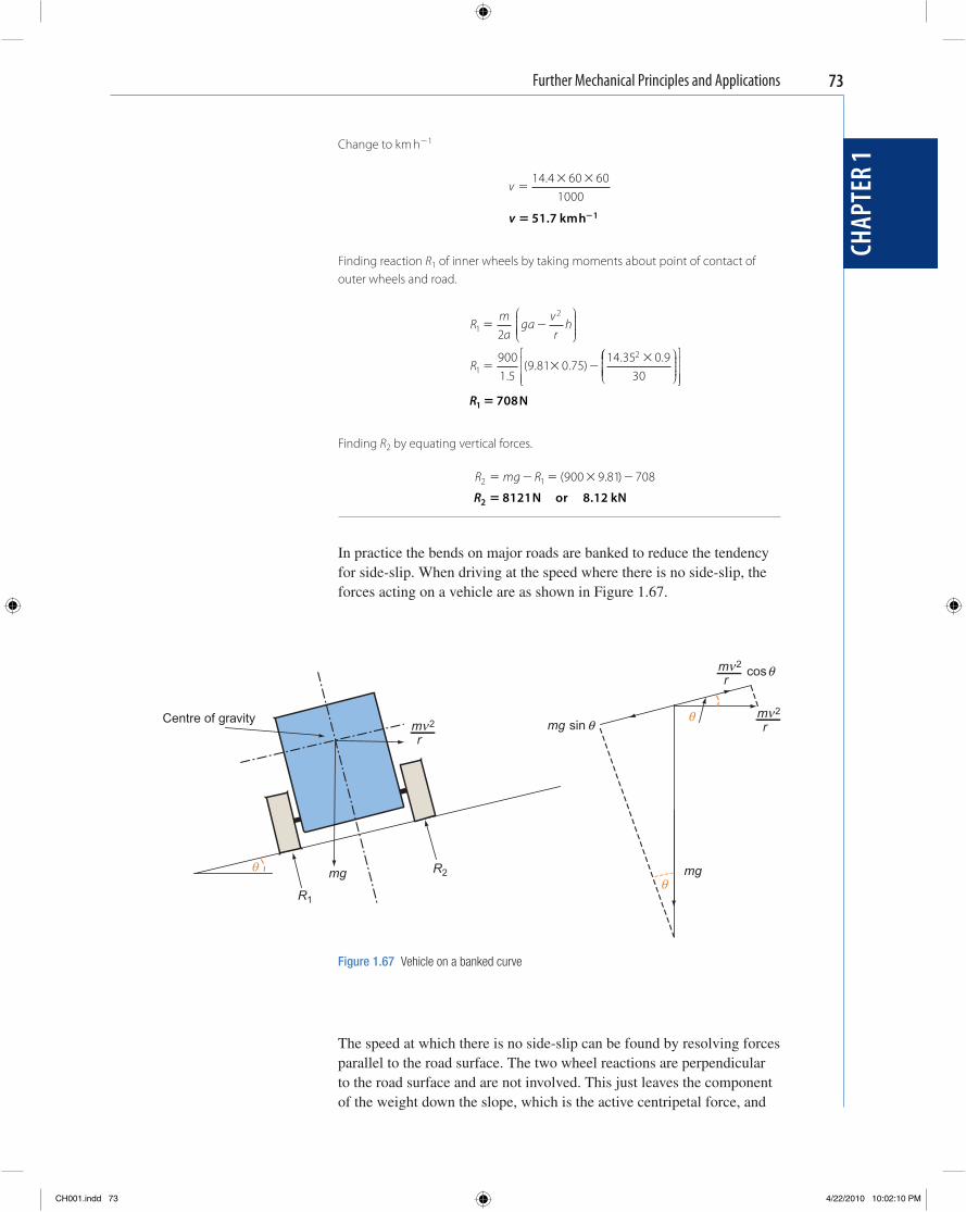
Further Mechanical Principles and Applications
CHAP
TER
1
73
Change to km h � 1
v �
� �14 4 60 601000
.
v � �51 7 1. kmh
Finding reaction R 1 of inner wheels by taking moments about point of contact of outer wheels and road.
Rm
aga
vr
h
R
1
2
1
2
2
9001 5
9 81 0 7514 35 0 9
30
� �
� � ��
⎛
⎝⎜⎜⎜⎜
⎞
⎠⎟⎟⎟⎟
.( . . )
. .⎛⎛
⎝⎜⎜⎜⎜
⎞
⎠⎟⎟⎟⎟
⎡
⎣⎢⎢⎢
⎤
⎦⎥⎥⎥
R1 708� N
Finding R 2 by equating vertical forces.
R mg R2 1 900 9 81 708� � � � �( . )
R2 8121 8 12� N kNor .
In practice the bends on major roads are banked to reduce the tendency for side-slip. When driving at the speed where there is no side-slip, the forces acting on a vehicle are as shown in Figure 1.67 .
θ
θθ
Centre of gravitym 2
r
R2
R1
mg mg
θmg sin
cosθ
νm 2
rν
m 2
rν
Figure 1.67 Vehicle on a banked curve
The speed at which there is no side-slip can be found by resolving forces parallel to the road surface. The two wheel reactions are perpendicular to the road surface and are not involved. This just leaves the component of the weight down the slope, which is the active centripetal force, and
CH001.indd 73CH001.indd 73 4/22/2010 10:02:10 PM4/22/2010 10:02:10 PM
Further Mechanical Principles and Applications
CHAP
TER
174
the component of the centrifugal reaction up the slope. For no side-slip, these must be equal and opposite.
mv
rmg
v rg rg
2
2
cos sin
sin
costan
� �
��
�
�
� �
v rg� tan �
(1.70)
Example 1.30
A vehicle has a track width of 1.4 m and the height of its centre of gravity is 1.2 m above the road surface. The limiting coeffi cient of friction between the wheels and the road surface is 0.7.
(a) What is the maximum speed at which the vehicle can travel round a curve of radius 75 m?
(b) To what angle would the curve have to be banked for the vehicle to travel round it at a speed of 50 km h � 1 without any tendency to side-slip?
(a) Finding the ratio of half the track width to height of centre of gravity.
ah
� �0 71 2
0 583..
.
Comparing this with the coeffi cient of friction whose value is � � 0.7 shows that:
� >
ah
This indicates that the car will overturn before the skidding speed is reached.
Finding speed at which car can travel round the curve, i.e. when overturning is likely to occur.
v
ah
rg� � � �0 71 2
75 9 81..
.
v � �20 7 1. m s
Change to km h � 1
v �
� �20 7 60 601000
.
v � �74 6 1. kmh
Changing 50 km h � 1 to m s � 2
v �
�
�
50 100060 60
v � �13 9 1. m s
KEY POINT In the condition where there is no tendency for side-slip, the reactions of the inner and outer wheels are equal.
CH001.indd 74CH001.indd 74 4/22/2010 10:02:10 PM4/22/2010 10:02:10 PM
Further Mechanical Principles and Applications
CHAP
TER
1
75
? Test your knowledge 1.13 1. What effect does the mass of a vehicle have on the maximum speed at
which it can travel round a curve?
2. If ��ah
, is a vehicle likely to skid or overturn if its speed is
excessive?
3. How is the centripetal force provided when a car travels round an unbanked curve?
4. How is the centripetal force provided when a car travels round a banked curve?
(b) Finding angle to which curve would need to be banked for no side-slip at this speed.
v rg
v rg
vrg
�
�
� ��
�
tan
tan
tan
tan
�
�
�
�
2
2 213 975 9 81
0 262
..
. � � 14 7. �
Activity 1.12
A vehicle of mass 1 tonne travels round a horizontal unbanked curve of radius 35 m. The track width of the vehicle is 1.8 m and the height of its centre of gravity above the road surface is 0.95 m. The coeffi cient of friction between the tyres and the road is 0.65.
(a) Show that if the speed of the vehicle is excessive, it is likely to skid rather than overturn.
(b) Calculate the speed at which skidding is likely to occur. (c) Calculate the reactions of the inner and outer wheels at this speed. (d) If the curve were to be banked at an angle of 3.5 ° what would be the
speed at which the vehicle could travel around it without any tendency for side-slip?
To check your understanding of the preceding section, you can solve Review questions 40–44 at the end of this chapter.
Simple Machines
A simple machine is an arrangement of moving parts whose purpose is to transmit motion and force. The ones which we will consider are those in which a relatively small input force is used to raise a heavy load. They include lever systems, inclined planes, screw jacks, wheel and axle arrangements and gear trains ( Figure 1.68 ).
CH001.indd 75CH001.indd 75 4/22/2010 10:02:10 PM4/22/2010 10:02:10 PM
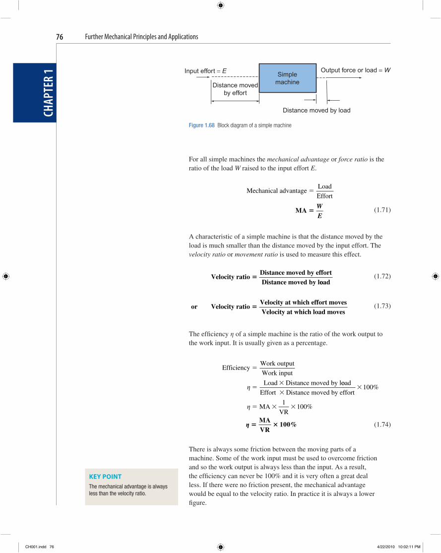
Further Mechanical Principles and Applications
CHAP
TER
176
For all simple machines the mechanical advantage or force ratio is the ratio of the load W raised to the input effort E .
Mechanical advantage
Load
Effort�
MA �
WE
(1.71)
A characteristic of a simple machine is that the distance moved by the load is much smaller than the distance moved by the input effort. The velocity ratio or movement ratio is used to measure this effect.
Velocity ratio
Distance moved by effortDistance moved by l
�ooad
(1.72)
or Velocity ratioVelocity at which effort movesVelocity at
� which load moves
(1.73)
The effi ciency � of a simple machine is the ratio of the work output to the work input. It is usually given as a percentage.
EfficiencyWork output
Work input
Load Distance moved by l
�
��
�ooad
Effort Distance moved by effort
MAVR
��
� � �
100
1100
%
%�
� � �
MAVR
100%
(1.74)
There is always some friction between the moving parts of a machine. Some of the work input must be used to overcome friction and so the work output is always less than the input. As a result, the effi ciency can never be 100% and it is very often a great deal less. If there were no friction present, the mechanical advantage would be equal to the velocity ratio. In practice it is always a lower fi gure.
Simplemachine
Input effort = E
Distance movedby effort
Distance moved by load
Output force or load = W
Figure 1.68 Block diagram of a simple machine
KEY POINT The mechanical advantage is always less than the velocity ratio.
CH001.indd 76CH001.indd 76 4/22/2010 10:02:11 PM4/22/2010 10:02:11 PM
Further Mechanical Principles and Applications
CHAP
TER
1
77
Example 1.31
A jack requires an input eff ort of 25 N to raise a load of 150 kg. If the distance moved by the eff ort is 500 mm and the load is raised through a height of 6 mm fi nd (a) the mechanical advantage, (b) the velocity ratio, (c) the effi ciency, (d) the work done in overcoming friction.
(a) Finding mechanical advantage.
MA
LoadEffort
� ��150 9 8125
.
MA � 58 9.
(b) Finding velocity ratio.
VR
Distance moved by effortDistance moved by load
� �500
6
VR � 83 3.
(c) Finding effi ciency.
� � � �
MAVR
58 983 3
100..
%
� � 70 7. %
(d) Finding work done in overcoming friction.
The work output is 70.7% of the work input. The remaining 29.3% of the work input is the work done in overcoming friction.
Work done in overcoming friction Work input
Work do
� �29 3100
.
nne in overcoming friction Effort Distance effort moves� � �29..
..
3100
25 0 529 3100
Work done in overcoming friction � � �
Work done in overcoming friction J� 3 66.
Velocity ratio formulae
The expressions (1.72) and (1.73) are general formulae for calculating velocity ratio and these can now be applied to a range of devices. Each will then have its own particular formula for velocity ratio which is dependent upon its dimensions and its mode of operation. For each device let the distance moved by the effort be a and the corresponding distance moved by the load be b .
i.e. Velocity ratio
Distance moved by effort
Distance moved�
by load
VR �
ab
(1.75)
CH001.indd 77CH001.indd 77 4/22/2010 10:02:11 PM4/22/2010 10:02:11 PM
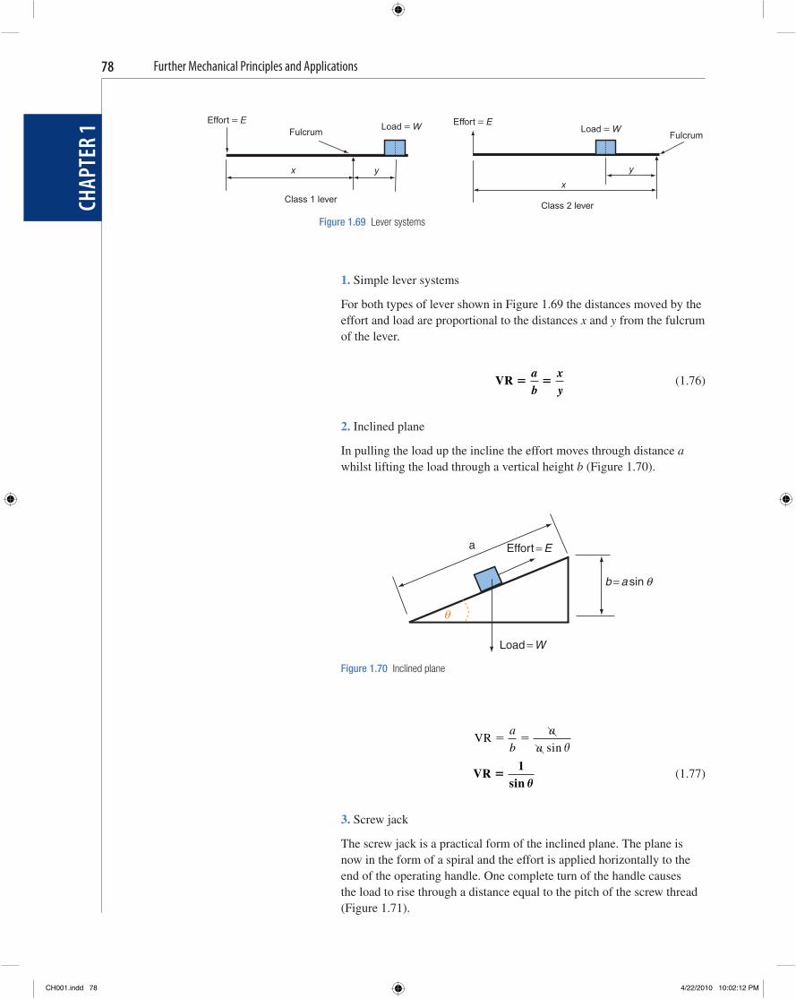
Further Mechanical Principles and Applications
CHAP
TER
178
1. Simple lever systems
For both types of lever shown in Figure 1.69 the distances moved by the effort and load are proportional to the distances x and y from the fulcrum of the lever.
VR � �
ab
xy
(1.76)
2. Inclined plane
In pulling the load up the incline the effort moves through distance a whilst lifting the load through a vertical height b ( Figure 1.70 ).
VR
sin� �
a
b
a
a �
VR
sin�
1�
(1.77)
3. Screw jack
The screw jack is a practical form of the inclined plane. The plane is now in the form of a spiral and the effort is applied horizontally to the end of the operating handle. One complete turn of the handle causes the load to rise through a distance equal to the pitch of the screw thread ( Figure 1.71 ).
Effort = E Effort = E Fulcrum Fulcrum
Load = W Load = W
Class 1 leverClass 2 lever
x
x
y y
Figure 1.69 Lever systems
a Effort = E
b = a sin θ
θ
Load = W
Figure 1.70 Inclined plane
CH001.indd 78CH001.indd 78 4/22/2010 10:02:12 PM4/22/2010 10:02:12 PM
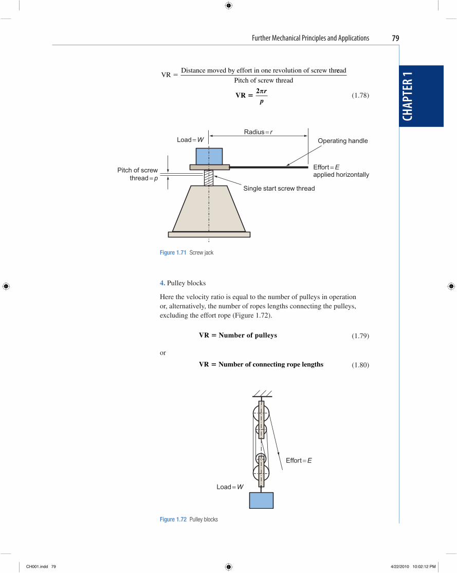
Further Mechanical Principles and Applications
CHAP
TER
1
79
.
Effort = E
Load = W
Figure 1.72 Pulley blocks
VR
Distance moved by effort in one revolution of screw thr�
eead
Pitch of screw thread
VR �
2�rp
(1.78)
Radius = rOperating handle
Pitch of screwthread = p
Effort = Eapplied horizontally
Single start screw thread
Load = W
Figure 1.71 Screw jack
4. Pulley blocks
Here the velocity ratio is equal to the number of pulleys in operation or, alternatively, the number of ropes lengths connecting the pulleys, excluding the effort rope ( Figure 1.72 ).
VR Number of pulleys�
(1.79)
or
VR Number of connecting rope lengths�
(1.80)
CH001.indd 79CH001.indd 79 4/22/2010 10:02:12 PM4/22/2010 10:02:12 PM
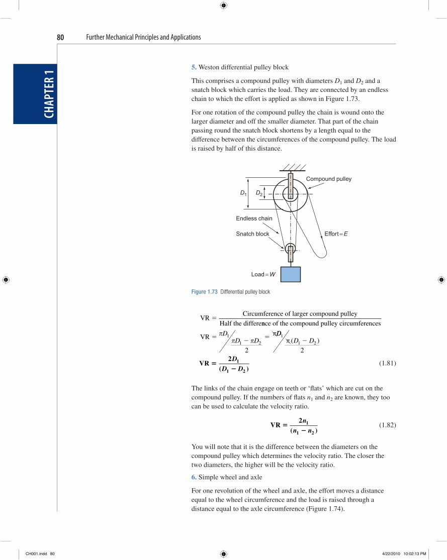
Further Mechanical Principles and Applications
CHAP
TER
180
5. Weston differential pulley block
This comprises a compound pulley with diameters D 1 and D 2 and a snatch block which carries the load. They are connected by an endless chain to which the effort is applied as shown in Figure 1.73 .
For one rotation of the compound pulley the chain is wound onto the larger diameter and off the smaller diameter. That part of the chain passing round the snatch block shortens by a length equal to the difference between the circumferences of the compound pulley. The load is raised by half of this distance.
Compound pulley
D1 D2
Endless chain
Snatch block Effort = E
Load = W
Figure 1.73 Differential pulley block
VRCircumference of larger compound pulley
Half the differe�
nnce of the compound pulley circumferences
VR ��
��
� ��D
D D1
1 2
2
DDD D
1
1 2
2
� ( )�
VR �
�
2 1
1 2
D
D D( ) (1.81)
The links of the chain engage on teeth or ‘ fl ats ’ which are cut on the compound pulley. If the numbers of fl ats n 1 and n 2 are known, they too can be used to calculate the velocity ratio.
VR �
�
2 1
1 2
n
n n( ) (1.82)
You will note that it is the difference between the diameters on the compound pulley which determines the velocity ratio. The closer the two diameters, the higher will be the velocity ratio.
6. Simple wheel and axle
For one revolution of the wheel and axle, the effort moves a distance equal to the wheel circumference and the load is raised through a distance equal to the axle circumference ( Figure 1.74 ).
CH001.indd 80CH001.indd 80 4/22/2010 10:02:13 PM4/22/2010 10:02:13 PM
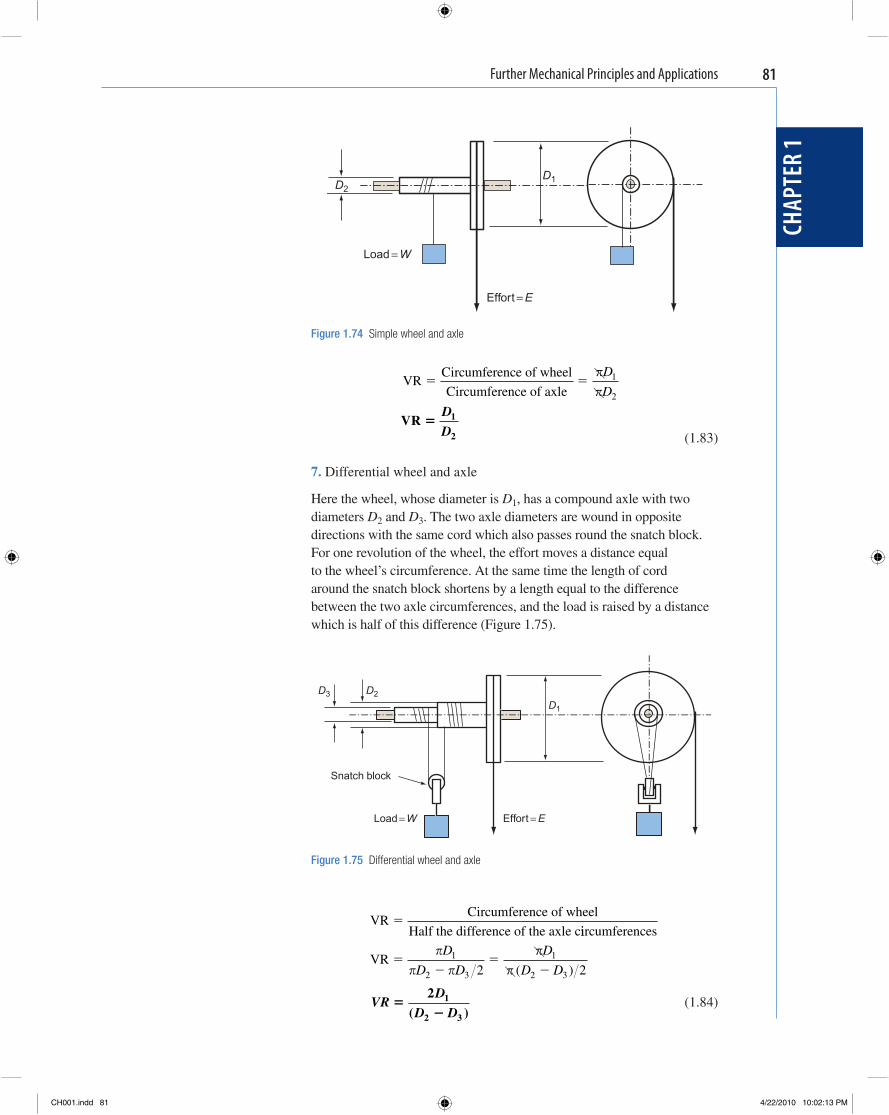
Further Mechanical Principles and Applications
CHAP
TER
1
81
VR
Circumference of wheel
Circumference of axle� �
��
D
D1
2
VR �
D
D1
2 (1.83)
7. Differential wheel and axle
Here the wheel, whose diameter is D 1 , has a compound axle with two diameters D 2 and D 3 . The two axle diameters are wound in opposite directions with the same cord which also passes round the snatch block. For one revolution of the wheel, the effort moves a distance equal to the wheel ’ s circumference. At the same time the length of cord around the snatch block shortens by a length equal to the difference between the two axle circumferences, and the load is raised by a distance which is half of this difference ( Figure 1.75 ).
D3 D2
D1
Snatch block
Load = W Effort = E
Figure 1.75 Differential wheel and axle
D2D1
Load = W
Effort = E
Figure 1.74 Simple wheel and axle
VRCircumference of wheel
Half the difference of the axle c�
iircumferences
VR ��
��
�� �
��
D
D D
D
D D1
2 3
1
2 32 2( )
VR
D
D D�
�
2 1
2 3( ) (1.84)
CH001.indd 81CH001.indd 81 4/22/2010 10:02:13 PM4/22/2010 10:02:13 PM
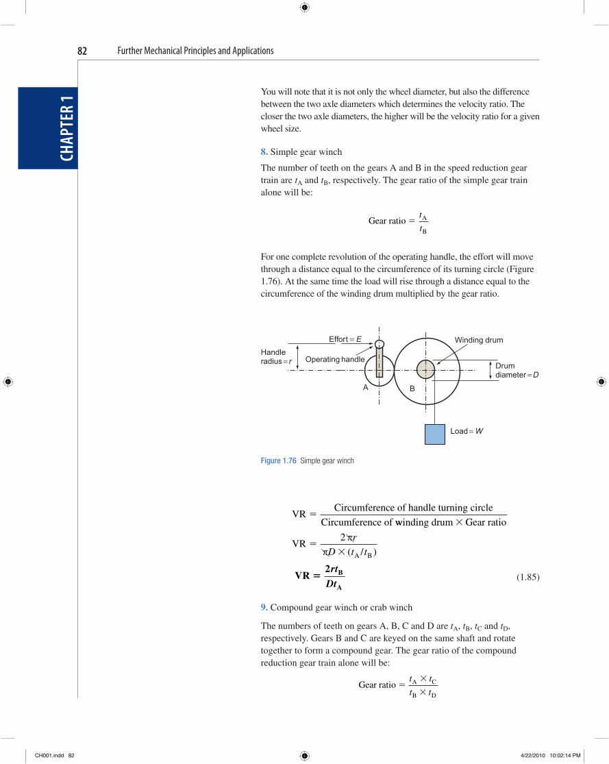
Further Mechanical Principles and Applications
CHAP
TER
182
You will note that it is not only the wheel diameter, but also the difference between the two axle diameters which determines the velocity ratio. The closer the two axle diameters, the higher will be the velocity ratio for a given wheel size.
8. Simple gear winch
The number of teeth on the gears A and B in the speed reduction gear train are t A and t B , respectively. The gear ratio of the simple gear train alone will be:
Gear ratio A
B
�t
t
For one complete revolution of the operating handle, the effort will move through a distance equal to the circumference of its turning circle (Figure 1.76). At the same time the load will rise through a distance equal to the circumference of the winding drum multiplied by the gear ratio.
Effort = E Winding drum
Handle radius = r Operating handle
Drum diameter = D
A
Load = W
B
Figure 1.76 Simple gear winch
VRCircumference of handle turning circle
Circumference of �
wwinding drum Gear ratio
VRA B
�
��
2 ��
r
D t t( / )
VR B
A
�2rt
Dt (1.85)
9. Compound gear winch or crab winch
The numbers of teeth on gears A, B, C and D are t A , t B , t C and t D , respectively. Gears B and C are keyed on the same shaft and rotate together to form a compound gear. The gear ratio of the compound reduction gear train alone will be:
Gear ratio A C
B D
��
�
t t
t t
CH001.indd 82CH001.indd 82 4/22/2010 10:02:14 PM4/22/2010 10:02:14 PM
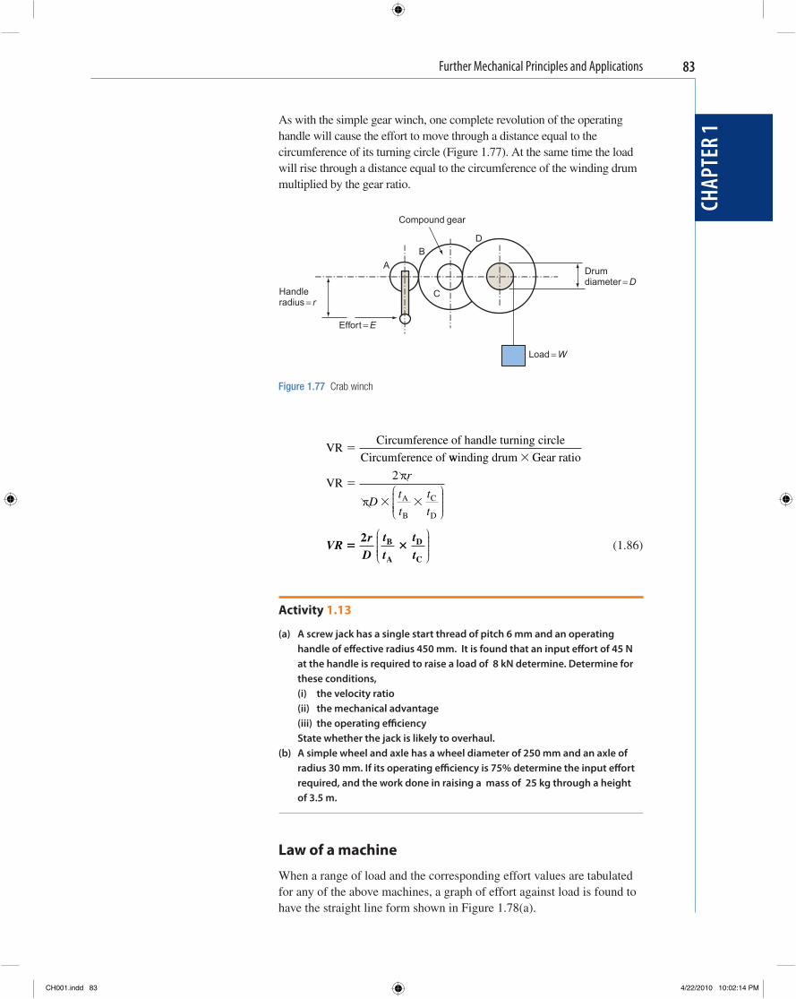
Further Mechanical Principles and Applications
CHAP
TER
1
83
As with the simple gear winch, one complete revolution of the operating handle will cause the effort to move through a distance equal to the circumference of its turning circle (Figure 1.77). At the same time the load will rise through a distance equal to the circumference of the winding drum multiplied by the gear ratio.
Compound gear
DB
A
Handle radius = r
Effort = E
C
Drum diameter = D
Load = W
Figure 1.77 Crab winch
VRCircumference of handle turning circle
Circumference of �
wwinding drum Gear ratio
VRA
B
C
D
�
�
� �
2 �
�
r
Dt
t
t
t
⎛
⎝⎜⎜⎜⎜
⎞
⎠⎟⎟⎟⎟
VR
rD
t
t
t
t� �
2 B
A
D
C
⎛
⎝⎜⎜⎜⎜
⎞
⎠⎟⎟⎟⎟
(1.86)
Activity 1.13
(a) A screw jack has a single start thread of pitch 6 mm and an operating handle of eff ective radius 450 mm. It is found that an input eff ort of 45 N at the handle is required to raise a load of 8 kN determine. Determine for these conditions,(i) the velocity ratio(ii) the mechanical advantage (iii) the operating effi ciencyState whether the jack is likely to overhaul.
(b) A simple wheel and axle has a wheel diameter of 250 mm and an axle of radius 30 mm. If its operating effi ciency is 75% determine the input eff ort required, and the work done in raising a mass of 25 kg through a height of 3.5 m.
Law of a machine
When a range of load and the corresponding effort values are tabulated for any of the above machines, a graph of effort against load is found to have the straight line form shown in Figure 1.78(a) .
CH001.indd 83CH001.indd 83 4/22/2010 10:02:14 PM4/22/2010 10:02:14 PM
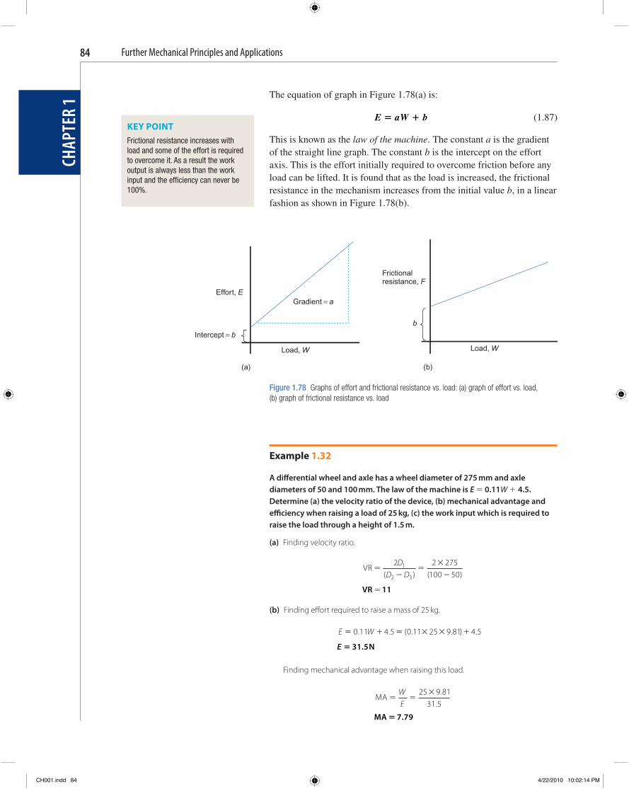
Further Mechanical Principles and Applications
CHAP
TER
184
The equation of graph in Figure 1.78(a) is:
E aW b� � (1.87)
This is known as the law of the machine . The constant a is the gradient of the straight line graph. The constant b is the intercept on the effort axis. This is the effort initially required to overcome friction before any load can be lifted. It is found that as the load is increased, the frictional resistance in the mechanism increases from the initial value b , in a linear fashion as shown in Figure 1.78(b) .
Frictionalresistance, F
Effort, EGradient = a
b
Intercept = b
Load, W Load, W
(a) (b)
Figure 1.78 Graphs of effort and frictional resistance vs. load: (a) graph of effort vs. load, (b) graph of frictional resistance vs. load
KEY POINT Frictional resistance increases with load and some of the effort is required to overcome it. As a result the work output is always less than the work input and the effi ciency can never be 100%.
Example 1.32
A diff erential wheel and axle has a wheel diameter of 275 mm and axle diameters of 50 and 100 mm. The law of the machine is E � 0.11 W � 4.5. Determine (a) the velocity ratio of the device, (b) mechanical advantage and effi ciency when raising a load of 25 kg, (c) the work input which is required to raise the load through a height of 1.5 m.
(a) Finding velocity ratio.
VR �
��
�
�
2 2 275100 50
1
2 3
DD D( ) ( )
VR � 11
(b) Finding eff ort required to raise a mass of 25 kg.
E W� � � � � �0 11 4 5 0 11 25 9 81 4 5. . ( . . ) .
E � 31 5. N
Finding mechanical advantage when raising this load.
MA � �
�WE
25 9 8131 5
..
MA � 7 79.
CH001.indd 84CH001.indd 84 4/22/2010 10:02:14 PM4/22/2010 10:02:14 PM
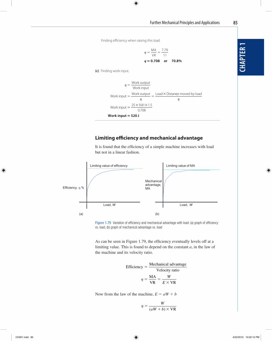
Further Mechanical Principles and Applications
CHAP
TER
1
85
Limiting value of efficiency Limiting value of MA
Mechanicaladvantage,MAEfficiency, h %
Load, W Load, W
(a) (b)
Figure 1.79 Variation of effi ciency and mechanical advantage with load: (a) graph of effi ciency vs. load, (b) graph of mechanical advantage vs. load
Finding effi ciency when raising this load.
� � �
MAVR
7 7911.
� � 0 708 70 8. or . %
(c) Finding work input.
�
�
�
� ��
Work outputWork input
Work inputWork output Load Distancce moved by load
Work input
�
�� �25 9 81 1 5
0 708. .
.
Work input J� 520
Limiting effi ciency and mechanical advantage
It is found that the effi ciency of a simple machine increases with load but not in a linear fashion.
As can be seen in Figure 1.79 , the effi ciency eventually levels off at a limiting value. This is found to depend on the constant a , in the law of the machine and its velocity ratio.
EfficiencyMechanical advantage
Velocity ratio
MA
VR VR
�
� ��
�W
E
Now from the law of the machine, E � aW � b
� �
� �
W
aW b( ) VR
CH001.indd 85CH001.indd 85 4/22/2010 10:02:15 PM4/22/2010 10:02:15 PM
Further Mechanical Principles and Applications
CHAP
TER
186
Dividing numerator and denominator by W gives:
� �
� �
1
ab
W
⎛⎝⎜⎜⎜
⎞⎠⎟⎟⎟⎟ VR
� �
�
1
ab
WVR VR
(1.88)
Examination of this expression shows that as the load W increases, the second term in the denominator becomes smaller and smaller. When the load becomes very large, this term tends to zero and the limiting value of effi ciency is:
� �
1a VR
(1.89)
In this limiting condition the mechanical advantage levels off to a value given by:
�
�
�
� �
MA
VRMA VR
MA �
1a
(1.90)
The limiting value of mechanical advantage is thus the reciprocal of the gradient of the effort vs. load graph.
Overhauling A simple machine is said to overhaul if when the effort is removed, the load falls under the effects of gravity. If a machine does not overhaul, then friction alone must be suffi cient to support the load. If you have changed a wheel on a car you probably used a screw jack to raise the wheel off the road surface. Friction in the screw thread is then suffi cient to support the car. This means, of course, that there must be quite a lot of friction present which results in a low value of effi ciency. This however is the price that often has to be paid for safety in lifting devices such as car jacks and engine hoists.
Frictional resistance can be considered as an additional load which the effort must overcome.
Total effort Effort to overcome friction load, ffort t
�
� �
Foo overcome actual load, W
Now in an ideal machine where there is no friction, the mechanical advantage is equal to the velocity ratio and,
VR MALoad
Effort
and EffortLoad
VR VR
� �
� �W
KEY POINT The mechanical advantage and the effi ciency of a simple machine increase with load but eventually level off at a limiting value.
CH001.indd 86CH001.indd 86 4/22/2010 10:02:16 PM4/22/2010 10:02:16 PM
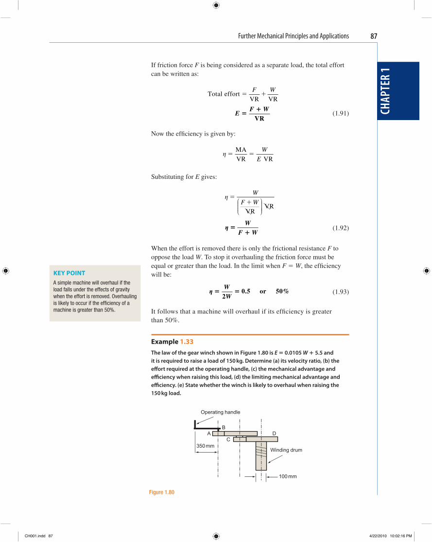
Further Mechanical Principles and Applications
CHAP
TER
1
87
KEY POINT A simple machine will overhaul if the load falls under the effects of gravity when the effort is removed. Overhauling is likely to occur if the effi ciency of a machine is greater than 50%.
Operating handle
BA D
C350 mm
Winding drum
100 mm
Figure 1.80
If friction force F is being considered as a separate load, the total effort can be written as:
Total effort
VR VR� �
F W
E
F W�
�
VR (1.91)
Now the effi ciency is given by:
� � �
MA
VR VR
W
E
Substituting for E gives:
� ��
W
F W
VRVR
⎛
⎝⎜⎜⎜
⎞
⎠⎟⎟⎟⎟
� �
�
WF W
(1.92)
When the effort is removed there is only the frictional resistance F to oppose the load W . To stop it overhauling the friction force must be equal or greater than the load. In the limit when F � W , the effi ciency will be:
� � �
WW2
0 5 50. or %
(1.93)
It follows that a machine will overhaul if its effi ciency is greater than 50%.
Example 1.33 The law of the gear winch shown in Figure 1.80 is E � 0. 0105 W � 5.5 and it is required to raise a load of 150 kg. Determine (a) its velocity ratio, (b) the eff ort required at the operating handle, (c) the mechanical advantage and effi ciency when raising this load, (d) the limiting mechanical advantage and effi ciency. (e) State whether the winch is likely to overhaul when raising the 150 kg load.
CH001.indd 87CH001.indd 87 4/22/2010 10:02:16 PM4/22/2010 10:02:16 PM
Further Mechanical Principles and Applications
CHAP
TER
188
? Test your knowledge 1.14
1. How does the mechanical advantage of a simple machine vary with the load raised?
2. How does the frictional resistance in a simple machine vary with the load raised?
3. How is the effi ciency of a simple machine defi ned? 4. What information does the law of a machine contain? 5. What is meant by overhauling and how can it be predicted?
Teeth on gear A 16�
�
�
Teeth on gear BTeeth on gear CTeet
7218
hh on gear D � 60
(a) Finding velocity ratio.
VR B
A
D
C
� � �� �
�
2 2 350100
72 6016 18
rD
tt
tt
⎛
⎝⎜⎜⎜⎜
⎞
⎠⎟⎟⎟⎟⎟
⎛⎝⎜⎜⎜
⎞⎠⎟⎟⎟⎟
VR � 105
(b) Finding eff ort required.
E W� � � � � �0 0105 5 5 0 0105 150 9 81 5 5. . ( . . ) .
E � 21 0. N
Finding mechanical advantage.
MA � �
�WE
150 9 8121 0
..
MA � 70 1.
Finding effi ciency.
� � �
MAVR
70 1105
.
� � 0 668 66 8. or . %
(c) Finding limiting mechanical advantage.
Limiting MA where from the law of the machine� �
10 0105
aa( . , ))
Limiting MA � �
10 0105
95 2.
.
Finding limiting effi ciency.
Limiting
VR� �
1a
Limiting � �
��
10 0105 105
0 907 90 7.
. or . %
(d) When raising the 150 kg load the effi ciency is greater than 50% and so the winch
will overhaul under these conditions.
CH001.indd 88CH001.indd 88 4/22/2010 10:02:16 PM4/22/2010 10:02:16 PM
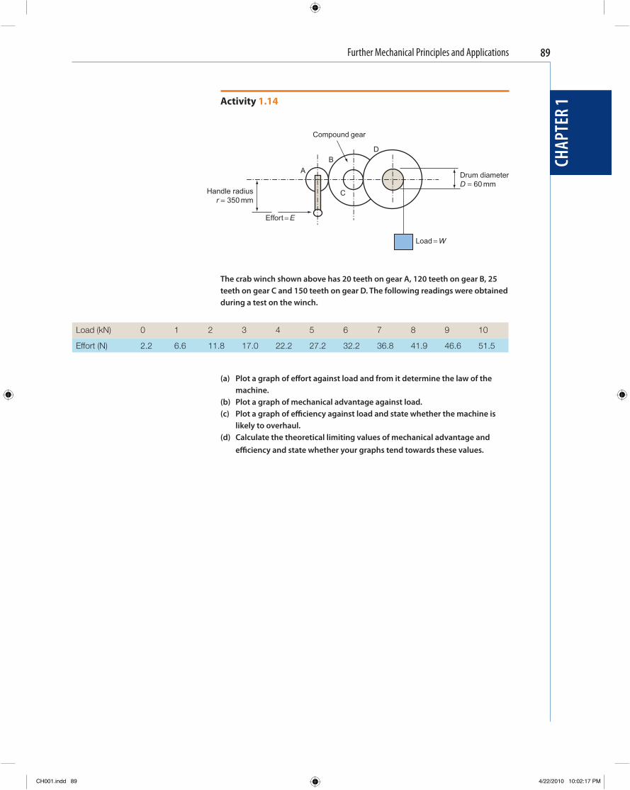
Further Mechanical Principles and Applications
CHAP
TER
1
89
Activity 1.14
Compound gear
DB
A
Handle radiusr = 350 mm
Effort = E
C
Drum diameterD = 60 mm
Load = W
The crab winch shown above has 20 teeth on gear A, 120 teeth on gear B, 25 teeth on gear C and 150 teeth on gear D. The following readings were obtained during a test on the winch.
Load (kN) 0 1 2 3 4 5 6 7 8 9 10
Effort (N) 2.2 6.6 11.8 17.0 22.2 27.2 32.2 36.8 41.9 46.6 51.5
(a) Plot a graph of eff ort against load and from it determine the law of the machine.
(b) Plot a graph of mechanical advantage against load. (c) Plot a graph of effi ciency against load and state whether the machine is
likely to overhaul. (d) Calculate the theoretical limiting values of mechanical advantage and
effi ciency and state whether your graphs tend towards these values.
CH001.indd 89CH001.indd 89 4/22/2010 10:02:17 PM4/22/2010 10:02:17 PM
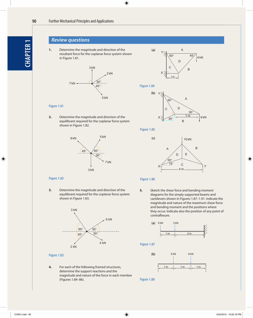
CHAP
TER
1Further Mechanical Principles and Applications90
Review questions
1. Determine the magnitude and direction of the resultant force for the coplanar force system shown in Figure 1.81 .
5. Sketch the shear force and bending moment diagrams for the simply supported beams and cantilevers shown in Figures 1.87–1.91 . Indicate the magnitude and nature of the maximum shear force and bending moment and the positions where they occur. Indicate also the position of any point of contrafl exure.
60° 30°
45° 30°
3 kN
6 kN
4 kN2 kN
Figure 1.83
3 kN
2 kN
7 kN 30°45°
5 kN
Figure 1.81
8 kN 5 kN
45° 60°30°
7 kN
3 kN
Figure 1.82
2. Determine the magnitude and direction of the equilibrant required for the coplanar force system shown in Figure 1.82 .
3. Determine the magnitude and direction of the equilibrant required for the coplanar force system shown in Figure 1.83 .
4. For each of the following framed structures, determine the support reactions and the magnitude and nature of the force in each member ( Figures 1.84–86 ).
Figure 1.84
Y60° 45°
4 kN
X1 m
A
BC
D
Figure 1.85
Y
30°
30°1 mX 30° 6 kN
A
C D
B
Figure 1.86
10 kN
15°30°
X Y4 m
A B
C
D E
Figure 1.87
5 kN 3 kN
1 m 2 m
Figure 1.88
5 kN 8 kN
1 m 1 m 1 m
(a)
(b)
(c)
(a)
(b)
CH001.indd 90CH001.indd 90 4/22/2010 10:02:18 PM4/22/2010 10:02:18 PM
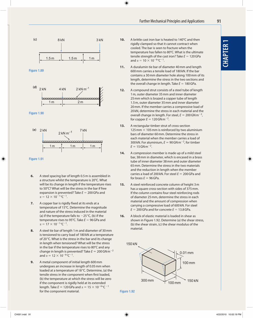
CHAP
TER
1
Further Mechanical Principles and Applications 91
6. A steel spacing bar of length 0.5 m is assembled in a structure whilst the temperature is 20°C. What will be its change in length if the temperature rises to 50°C? What will be the stress in the bar if free expansion is prevented? Take E � 200 GPa and � � 12 � 10 � 1 °C � 1 .
7. A copper bar is rigidly fi xed at its ends at a temperature of 15°C. Determine the magnitude and nature of the stress induced in the material (a) if the temperature falls to � 25 °C, (b) if the temperature rises to 95°C. Take E � 96 GPa and � � 17 � 10 � 1 °C � 1 .
8. A steel tie bar of length 1 m and diameter of 30 mm is tensioned to carry load of 180 kN at a temperature of 20 °C. What is the stress in the bar and its change in length when tensioned? What will be the stress in the bar if the temperature rises to 80°C and any change in length is prevented? Take E � 200 GN m � 2 and � � 12 � 10 � 6 °C � 1 .
9. A metal component of initial length 600 mm undergoes an increase in length of 0.05 mm when loaded at a temperature of 18 °C. Determine, (a) the tensile stress in the component when fi rst loaded, (b) the temperature at which the stress will be zero if the component is rigidly held at its extended length. Take E � 120 GPa and � � 15 � 10 � 6 °C � 1 for the component material.
10. A brittle cast iron bar is heated to 140°C and then rigidly clamped so that it cannot contract when cooled. The bar is seen to fracture when the temperature has fallen to 80°C. What is the ultimate tensile strength of the cast iron? Take E � 120 GPa and � � 10 � 10 � 6 °C � 1 .
11. A duralumin tie bar of diameter 40 mm and length 600 mm carries a tensile load of 180 kN. If the bar contains a 30 mm diameter hole along 100 mm of its length, determine the stress in the two sections and the overall change in length. Take E � 180 GPa.
12. A compound strut consists of a steel tube of length 1 m, outer diameter 35 mm and inner diameter 25 mm which is brazed a copper tube of length 1.5 m, outer diameter 35 mm and inner diameter 20 mm. If the member carries a compressive load of 20 kN, determine the stress in each material and the overall change in length. For steel, E � 200 GN m � 2 , for copper E � 120 GN m � 2 .
13. A rectangular timber strut of cross-section 125 mm � 105 mm is reinforced by two aluminium bars of diameter 60 mm. Determine the stress in each material when the member carries a load of 300 kN. For aluminium, E � 90 GN m � 2 , for timber E � 15 GN m � 2 .
14. A compression member is made up of a mild steel bar, 38 mm in diameter, which is encased in a brass tube of inner diameter 38 mm and outer diameter 65 mm. Determine the stress in the two materials and the reduction in length when the member carries a load of 200 kN. For steel E � 200 GPa and for brass E � 96 GPa.
15. A steel reinforced concrete column of height 3 m has a square cross-section with sides of 375 mm. If the column contains four steel reinforcing rods of diameter 25 mm, determine the stress in each material and the amount of compression when carrying a compressive load of 600 kN. For steel E � 200 GPa and for concrete E � 13.8 GPa.
16. A block of elastic material is loaded in shear as shown in Figure 1.92 . Determine (a) the shear stress, (b) the shear strain, (c) the shear modulus of the material.
Figure 1.89
8 kN 3 kN
1.5 m 1.5 m 1 m
Figure 1.90
2 kN 4 kN 2 kN m−1
1 m 2 m
Figure 1.91
2 kN 2 kN m−1 7 kN
1 m 1 m 1 m
100 mm300 mm
150 kN
150 kN
0.01 mm
100 mm
Figure 1.92
(c)
(d)
(e)
CH001.indd 91CH001.indd 91 4/22/2010 10:02:19 PM4/22/2010 10:02:19 PM
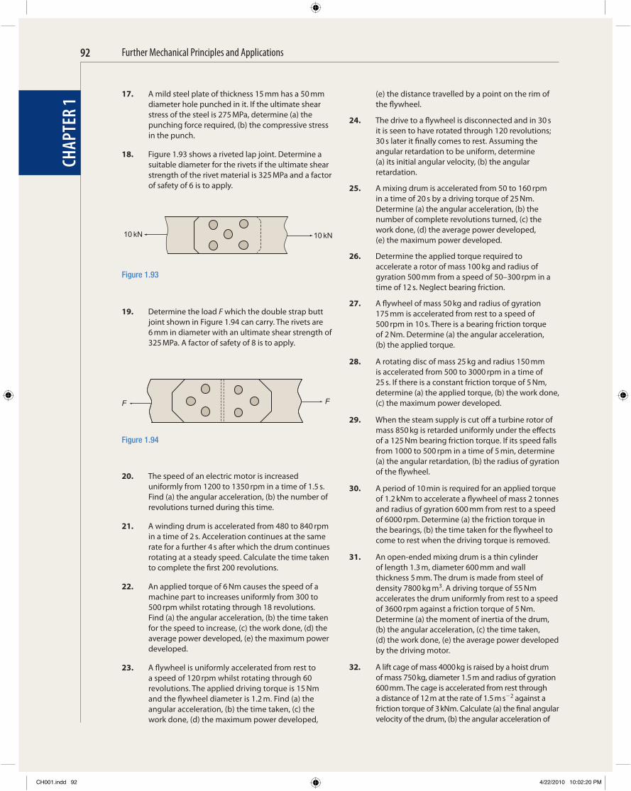
CHAP
TER
1Further Mechanical Principles and Applications92
(e) the distance travelled by a point on the rim of the fl ywheel.
24. The drive to a fl ywheel is disconnected and in 30 s it is seen to have rotated through 120 revolutions; 30 s later it fi nally comes to rest. Assuming the angular retardation to be uniform, determine (a) its initial angular velocity, (b) the angular retardation.
25. A mixing drum is accelerated from 50 to 160 rpm in a time of 20 s by a driving torque of 25 Nm. Determine (a) the angular acceleration, (b) the number of complete revolutions turned, (c) the work done, (d) the average power developed, (e) the maximum power developed.
26. Determine the applied torque required to accelerate a rotor of mass 100 kg and radius of gyration 500 mm from a speed of 50–300 rpm in a time of 12 s. Neglect bearing friction.
27. A fl ywheel of mass 50 kg and radius of gyration 175 mm is accelerated from rest to a speed of 500 rpm in 10 s. There is a bearing friction torque of 2 Nm. Determine (a) the angular acceleration, (b) the applied torque.
28. A rotating disc of mass 25 kg and radius 150 mm is accelerated from 500 to 3000 rpm in a time of 25 s. If there is a constant friction torque of 5 Nm, determine (a) the applied torque, (b) the work done, (c) the maximum power developed.
29. When the steam supply is cut off a turbine rotor of mass 850 kg is retarded uniformly under the eff ects of a 125 Nm bearing friction torque. If its speed falls from 1000 to 500 rpm in a time of 5 min, determine (a) the angular retardation, (b) the radius of gyration of the fl ywheel.
30. A period of 10 min is required for an applied torque of 1.2 kNm to accelerate a fl ywheel of mass 2 tonnes and radius of gyration 600 mm from rest to a speed of 6000 rpm. Determine (a) the friction torque in the bearings, (b) the time taken for the fl ywheel to come to rest when the driving torque is removed.
31. An open-ended mixing drum is a thin cylinder of length 1.3 m, diameter 600 mm and wall thickness 5 mm. The drum is made from steel of density 7800 kg m 3 . A driving torque of 55 Nm accelerates the drum uniformly from rest to a speed of 3600 rpm against a friction torque of 5 Nm. Determine (a) the moment of inertia of the drum, (b) the angular acceleration, (c) the time taken, (d) the work done, (e) the average power developed by the driving motor.
32. A lift cage of mass 4000 kg is raised by a hoist drum of mass 750 kg, diameter 1.5 m and radius of gyration 600 mm. The cage is accelerated from rest through a distance of 12 m at the rate of 1.5 m s � 2 against a friction torque of 3 kNm. Calculate (a) the fi nal angular velocity of the drum, (b) the angular acceleration of
17. A mild steel plate of thickness 15 mm has a 50 mm diameter hole punched in it. If the ultimate shear stress of the steel is 275 MPa, determine (a) the punching force required, (b) the compressive stress in the punch.
18. Figure 1.93 shows a riveted lap joint. Determine a suitable diameter for the rivets if the ultimate shear strength of the rivet material is 325 MPa and a factor of safety of 6 is to apply.
Figure 1.93
10 kN10 kN
19. Determine the load F which the double strap butt joint shown in Figure 1.94 can carry. The rivets are 6 mm in diameter with an ultimate shear strength of 325 MPa. A factor of safety of 8 is to apply.
Figure 1.94
F F
20. The speed of an electric motor is increased uniformly from 1200 to 1350 rpm in a time of 1.5 s. Find (a) the angular acceleration, (b) the number of revolutions turned during this time.
21. A winding drum is accelerated from 480 to 840 rpm in a time of 2 s. Acceleration continues at the same rate for a further 4 s after which the drum continues rotating at a steady speed. Calculate the time taken to complete the fi rst 200 revolutions.
22. An applied torque of 6 Nm causes the speed of a machine part to increases uniformly from 300 to 500 rpm whilst rotating through 18 revolutions. Find (a) the angular acceleration, (b) the time taken for the speed to increase, (c) the work done, (d) the average power developed, (e) the maximum power developed.
23. A fl ywheel is uniformly accelerated from rest to a speed of 120 rpm whilst rotating through 60 revolutions. The applied driving torque is 15 Nm and the fl ywheel diameter is 1.2 m. Find (a) the angular acceleration, (b) the time taken, (c) the work done, (d) the maximum power developed,
CH001.indd 92CH001.indd 92 4/22/2010 10:02:20 PM4/22/2010 10:02:20 PM
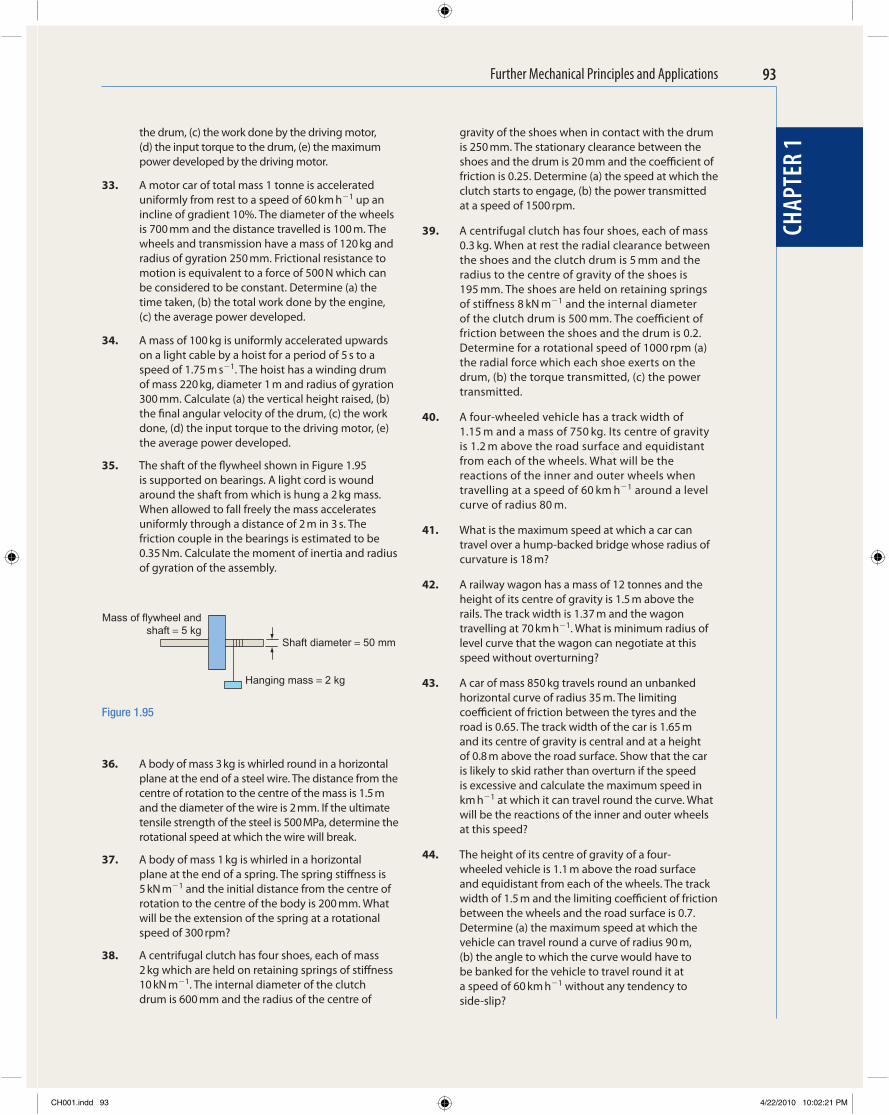
CHAP
TER
1
Further Mechanical Principles and Applications 93
the drum, (c) the work done by the driving motor, (d) the input torque to the drum, (e) the maximum power developed by the driving motor.
33. A motor car of total mass 1 tonne is accelerated uniformly from rest to a speed of 60 km h � 1 up an incline of gradient 10%. The diameter of the wheels is 700 mm and the distance travelled is 100 m. The wheels and transmission have a mass of 120 kg and radius of gyration 250 mm. Frictional resistance to motion is equivalent to a force of 500 N which can be considered to be constant. Determine (a) the time taken, (b) the total work done by the engine, (c) the average power developed.
34. A mass of 100 kg is uniformly accelerated upwards on a light cable by a hoist for a period of 5 s to a speed of 1.75 m s � 1 . The hoist has a winding drum of mass 220 kg, diameter 1 m and radius of gyration 300 mm. Calculate (a) the vertical height raised, (b) the fi nal angular velocity of the drum, (c) the work done, (d) the input torque to the driving motor, (e) the average power developed.
35. The shaft of the fl ywheel shown in Figure 1.95 is supported on bearings. A light cord is wound around the shaft from which is hung a 2 kg mass. When allowed to fall freely the mass accelerates uniformly through a distance of 2 m in 3 s. The friction couple in the bearings is estimated to be 0.35 Nm. Calculate the moment of inertia and radius of gyration of the assembly.
gravity of the shoes when in contact with the drum is 250 mm. The stationary clearance between the shoes and the drum is 20 mm and the coeffi cient of friction is 0.25. Determine (a) the speed at which the clutch starts to engage, (b) the power transmitted at a speed of 1500 rpm.
39. A centrifugal clutch has four shoes, each of mass 0.3 kg. When at rest the radial clearance between the shoes and the clutch drum is 5 mm and the radius to the centre of gravity of the shoes is 195 mm. The shoes are held on retaining springs of stiff ness 8 kN m � 1 and the internal diameter of the clutch drum is 500 mm. The coeffi cient of friction between the shoes and the drum is 0.2. Determine for a rotational speed of 1000 rpm (a) the radial force which each shoe exerts on the drum, (b) the torque transmitted, (c) the power transmitted.
40. A four-wheeled vehicle has a track width of 1.15 m and a mass of 750 kg. Its centre of gravity is 1.2 m above the road surface and equidistant from each of the wheels. What will be the reactions of the inner and outer wheels when travelling at a speed of 60 km h � 1 around a level curve of radius 80 m.
41. What is the maximum speed at which a car can travel over a hump-backed bridge whose radius of curvature is 18 m?
42. A railway wagon has a mass of 12 tonnes and the height of its centre of gravity is 1.5 m above the rails. The track width is 1.37 m and the wagon travelling at 70 km h � 1 . What is minimum radius of level curve that the wagon can negotiate at this speed without overturning?
43. A car of mass 850 kg travels round an unbanked horizontal curve of radius 35 m. The limiting coeffi cient of friction between the tyres and the road is 0.65. The track width of the car is 1.65 m and its centre of gravity is central and at a height of 0.8 m above the road surface. Show that the car is likely to skid rather than overturn if the speed is excessive and calculate the maximum speed in km h � 1 at which it can travel round the curve. What will be the reactions of the inner and outer wheels at this speed?
44. The height of its centre of gravity of a four-wheeled vehicle is 1.1 m above the road surface and equidistant from each of the wheels. The track width of 1.5 m and the limiting coeffi cient of friction between the wheels and the road surface is 0.7. Determine (a) the maximum speed at which the vehicle can travel round a curve of radius 90 m, (b) the angle to which the curve would have to be banked for the vehicle to travel round it at a speed of 60 km h � 1 without any tendency to side-slip?
Figure 1.95
Shaft diameter = 50 mm
Hanging mass = 2 kg
Mass of flywheel andshaft = 5 kg
36. A body of mass 3 kg is whirled round in a horizontal plane at the end of a steel wire. The distance from the centre of rotation to the centre of the mass is 1.5 m and the diameter of the wire is 2 mm. If the ultimate tensile strength of the steel is 500 MPa, determine the rotational speed at which the wire will break.
37. A body of mass 1 kg is whirled in a horizontal plane at the end of a spring. The spring stiff ness is 5 kN m � 1 and the initial distance from the centre of rotation to the centre of the body is 200 mm. What will be the extension of the spring at a rotational speed of 300 rpm?
38. A centrifugal clutch has four shoes, each of mass 2 kg which are held on retaining springs of stiff ness 10 kN m � 1 . The internal diameter of the clutch drum is 600 mm and the radius of the centre of
CH001.indd 93CH001.indd 93 4/22/2010 10:02:21 PM4/22/2010 10:02:21 PM
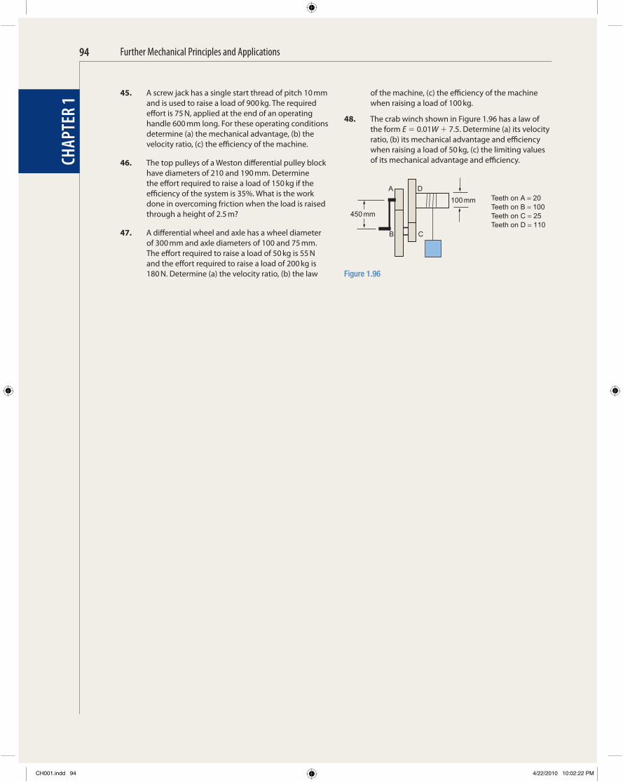
CHAP
TER
1Further Mechanical Principles and Applications94
45. A screw jack has a single start thread of pitch 10 mm and is used to raise a load of 900 kg. The required eff ort is 75 N, applied at the end of an operating handle 600 mm long. For these operating conditions determine (a) the mechanical advantage, (b) the velocity ratio, (c) the effi ciency of the machine.
46. The top pulleys of a Weston diff erential pulley block have diameters of 210 and 190 mm. Determine the eff ort required to raise a load of 150 kg if the effi ciency of the system is 35%. What is the work done in overcoming friction when the load is raised through a height of 2.5 m?
47. A diff erential wheel and axle has a wheel diameter of 300 mm and axle diameters of 100 and 75 mm. The eff ort required to raise a load of 50 kg is 55 N and the eff ort required to raise a load of 200 kg is 180 N. Determine (a) the velocity ratio, (b) the law
A D
100 mm
B C
450 mm
Teeth on A = 20Teeth on B = 100Teeth on C = 25Teeth on D = 110
Figure 1.96
of the machine, (c) the effi ciency of the machine when raising a load of 100 kg.
48. The crab winch shown in Figure 1.96 has a law of the form E � 0.01 W � 7.5. Determine (a) its velocity ratio, (b) its mechanical advantage and effi ciency when raising a load of 50 kg, (c) the limiting values of its mechanical advantage and effi ciency.
CH001.indd 94CH001.indd 94 4/22/2010 10:02:22 PM4/22/2010 10:02:22 PM

CH001.indd 95CH001.indd 95 4/22/2010 10:02:22 PM4/22/2010 10:02:22 PM