Future Directions of Electromagnetic Methodsfor Hydrocarbon Applications

K. M. Strack

Received: 11 October 2012 / Accepted: 22 April 2013 / Published online: 12 June 2013� Springer Science+Business Media Dordrecht 2013

Abstract For hydrocarbon applications, seismic exploration is the workhorse of the

industry. Only in the borehole, electromagnetic (EM) methods play a dominant role, as

they are mostly used to determine oil reserves and to distinguish water from oil-bearing

zones. Throughout the past 60 years, we had several periods with an increased interest in

EM. This increased with the success of the marine EM industry and now electromagnetics

in general is considered for many new applications. The classic electromagnetic methods

are borehole, onshore and offshore, and airborne EM methods. Airborne is covered else-

where (see Smith, this issue). Marine EM material is readily available from the service

company Web sites, and here I will only mention some future technical directions that are

visible. The marine EM success is being carried back to the onshore market, fueled by

geothermal and unconventional hydrocarbon applications. Oil companies are listening to

pro-EM arguments, but still are hesitant to go through the learning exercises as early

adopters. In particular, the huge business drivers of shale hydrocarbons and reservoir

monitoring will bring markets many times bigger than the entire marine EM market.

Additional applications include support for seismic operations, sub-salt, and sub-basalt, all

areas where seismic exploration is costly and inefficient. Integration with EM will allow

novel seismic methods to be applied. In the borehole, anisotropy measurements, now

possible, form the missing link between surface measurements and ground truth. Three-

dimensional (3D) induction measurements are readily available from several logging

contractors. The trend to logging-while-drilling measurements will continue with many

more EM technologies, and the effort of controlling the drill bit while drilling including

look-ahead-and-around the drill bit is going on. Overall, the market for electromagnetics is

increasing, and a demand for EM capable professionals will continue. The emphasis will

be more on application and data integration (bottom-line value increase) and less on EM

technology and modeling exercises.

IAGA 21st EM induction workshop Review Paper, Darwin, Australia, 2012.

K. M. Strack (&)KMS Technologies—KJT Enterprises Inc., 6420 Richmond Ave, Suite 610, Houston, TX 77077, USAe-mail: kurt@kmstechnologies.com

123

Surv Geophys (2014) 35:157–177DOI 10.1007/s10712-013-9237-z

Keywords Electromagnetics � Hydrocarbon exploration � Electrical geophysics

1 Introduction

Electrical methods in applied geophysics started along with the other geophysical methods

in the early 1900s with Wenner (1912), Schlumberger in 1922 (Gruner Schlumberger

1982) and early patents by Schilowsky (German patent 322040 assigned 1913), and Blau

(US patent 1911137 assigned 1933 to Standard Oil Development Corp.). Countless patents

have been filed since then, and the interest in electromagnetics has been growing steadily

except for onshore applications, where the interest was cyclical and a new cycle is just

starting. Hydrocarbon applications are always driven by commercial interests and com-

petitiveness and are thus cyclical. Understanding the market values and where values drive

the markets is almost as important as understanding the technical benefits of the individual

methods, because in many instances the market drives the technical priorities.

There are four principal areas for electromagnetics for hydrocarbon applications:

borehole, offshore, onshore and airborne. Airborne applications are covered by a separate

review paper (see Smith, this issue). For hydrocarbon exploration, airborne EM is limited

because of the depth of penetration although the depth has been extended to several

hundred meters in the past few years. A future market is its use for seismic static cor-

rections. During the 1990s, a revival in borehole electrical methods could be seen, and

while these technologies are now mature in the market place, derivatives for logging-

while-drilling applications are presently being developed. After 2000, there was a general

increase in marine electrical methods (Eidesmo et al. 2002) and after that technical bubble

burst. The market is now stable with a slowly growing trend. This is witnessed by stable

profitable business of the single dominant remaining market participant and only much

smaller acquisition participants and several interpretation shops. There has been little

change in land applications until recently, when interest increased. We now have at least 5

global service providers (Europe, Russia, China, and North America) that can handle small

to large land acquisition surveys. This is mostly driven by the marine success and estab-

lishing slowly the value of EM to address problems to seismic acquisition. This is wit-

nessed by the fact that three of the large EM land contractors are part of largest global

seismic service companies. New opportunities like monitoring and applications to shale

reserves are on the horizon (Kumar and Hoversten 2012; Strack and Aziz 2012).

Following in part from the tremendous progress in seismic methods, we have a great

deal of new technology (electronics, computing and workflow) at our fingertips. It thus is

reasonable to first understand the markets, starting with the most developed one:

• Borehole applications including all logging methods (wireline, logging-while-drilling,

production logging, cross-well). This is the most important market area for

electromagnetics (EM) as electrical logging tools are run in almost every well. The

global annual market is 1–2 billion US $ in services alone. In addition, there is a

50–100 million $ hardware market.

• Marine applications are more recent and present a stable industry that has demonstrated

its value to oil company customers. That global market in 2012 is approximately 200

million US $.

• Airborne applications to hydrocarbon exploration are limited to 10–20 million US $

annually because of the limited application scope (see Smith, R, review paper this

issue).

158 Surv Geophys (2014) 35:157–177

123

• Land applications, albeit growing, are only reaching approximately 50 million US $ in

2012 (excluding China and Russia).

The EM-related logging market is the only area that has continuously been growing in

market size and also in technology. This is related to improved technology (hardware and

software) that allows us to get more signal from the noise and thus higher reliable resistor

values (related to smaller signal) and directly in correlation is ‘More Oil’. Specifically,

operational decisions and reserve estimates are driving the use of EM. It thus makes sense

to define these technology development phases as baseline and gauge the other areas

accordingly.

Clear phases in borehole applications can be distinguished (Luthi 2001).

1921–1927 Conceptual phase

1927–1949 Acceptance phase

1949–1985 Maturity phase

1985–now Reinvention phase… maybe we are at its end

During the conceptual phase, the technology was invented and initially tested. Success

came only after it was taken to different countries from France and put on a broader basis.

During the acceptance phase, most electrical logging tools were developed in their basic

form and its use refined during the maturity phase. Then came logging-while-drilling,

which challenged the leadership of one company. The luster of having developed all

logging tools was destroyed by tools being developed under oil company sponsorship. (In

fact, many of the wireline tools during the 1980s and 1990s were developed with oil

company mentorship.) This is the direct result of the customer learning how to use the

technology and wanting his or her own implementations. Parallel to the development of

new wireline tools, logging-while-drilling tools were developed, but mostly on the basis of

getting a slight competitive advantage. Thus, in the logging-while-drilling market, the

dominance of an individual company is limited. Around 2010–2012, there is clearly a shift

happening, and it appears that we are entering a new era of acceptance of the technology

developed in the past 20 years.

Using this analogy for the marine electromagnetics industry, we can see that we are

almost at the end of the conceptual phase. Numerous marine technologies have been

developed, and only those that were operationally mature survive. Before the end of the

conceptual phase, there will be several more seismic integrated systems and the industry

will have more than just one contractor. This is because globally we see tenders from oil

companies that are requiring exactly what they need, which is not always what the service

industry provides or markets. Tenders for shallow water integrated seismic, marine mag-

netotellurics and even time domain electromagnetics are on the market while the offering

is predominantly frequency domain controlled-source electromagnetics. Needless to say,

the market will respond to demands and not only to offerings. In open competition, the

market always reaches a balance between technical and business aspects.

For onshore electrical methods, we already had two conceptual phases and are now in

the start of the third: One in the 1950s and one in the 1980s (during the latter period, most

presently used technology was developed). For hydrocarbon applications, only magneto-

tellurics made it to an acceptance and now into maturity. At the same time driven by the

success of the marine EM market and the borehole EM innovations, many novel market

players and novel applications are revisiting land technology. Most likely several of them

will become successful. Judging from the history in the borehole and marine (also air-

borne) fields, the winning player will be a newcomer.

Surv Geophys (2014) 35:157–177 159

123

Looking at these different phases explains why the reviewers of this subject matter in

the recent past (this means mostly for onshore) focused on a small aspect of hydrocarbon

applications as they were filling in the gap. The last broader hydrocarbon review was

written in a series of papers by Spies and Nekut (Nekut and Spies 1989; Spies 1983; Spies

and Frischknecht 1991). Other reviews focus on electrical methods in general and to a

small degree on hydrocarbon applications (Nabighian and Macnae 2005; Sheard et al.

2005). Numerous review papers have been offered on marine electromagnetics (Constable

and Srnka 2007; Constable 2010). The best source for review is presently the Web sites of

the marine contractors, which give links to the scientific papers about the technology they

use. Further information can be found in various reviews (i.e., Srnka et al. 2006; Constable

and Srnka 2007; Constable 2010).

I will here go through the applications in the above sequence and point out the

developments; I derive by considering the direction in which the industry might be

heading. I will combine business, history and technical aspects to derive market directions.

This path builds on the success of EM in the borehole, which is attributed to the solution of

real problems. The success of 3D induction log technology can be directly translated to

finding more reserves and not only the measurements delivering more complete images.

The same is true for marine Controlled-Source ElectroMagnetics (CSEM). On the other

side, Hesthammer has been advocating its use for making drilling decisions (Hesthammer

et al. 2010) and recently reported the confirmation of drilling results (Hesthammer et al.

2012) while not being a commercial success. In the context of drilling cost and decision,

the use of CSEM, even at low resolution using EM, is justifiable. Only for onshore

hydrocarbon applications have we yet to reach that point that has been reached several

times already in the conceptual phase.

Here, I caution the reader to take initial drilling success or failure as scientific proof as

more than just one method or approach contributes to drilling decisions: Only longer term

statistics can be the judge when complex decision trees are involved.

2 The Methods

In the 1980s, the basic borehole methods included induction logs (also known as con-

ductivity tools) and laterologs (also known as galvanic tools or resistivity tools). After the

introduction of the array induction tool at the end of the 1980s, numerous alternatives were

developed. The innovation spirit spilled over to array laterologs, log inversion, through-

casing resistivities and 3D induction. All of these were developed in the 1990 and came on

the market through the 1990s and 2000s (Strack et al. 1998). Concurrent with the wireline

development, logging-while-drilling tools progressed, and today almost all wireline

resistivity measurements are available as logging-while-drilling tools. The advantage of

this lies in getting the information from the borehole before a drilling mud invaded zone is

built up. The next challenge lies in looking ahead and around the drill bit and placing a

borehole correctly in the three-dimensional space.

The borehole tool market has for 60 years been driven by dominance of a single

company. Only with the introduction of new technology, namely logging-while-drilling in

the 1980s, this situation changed. Intellectual property, in particular patents, protected this

position. In fact, the strategy and cultures that exist today in the geoscience industry come

from the logging world. Patents are used as business tools and to protect investment more

than to enforce a technical point. This means that one may wait for a while before claiming

patent infringement just to make sure there is enough financial benefit to be gained.

160 Surv Geophys (2014) 35:157–177

123

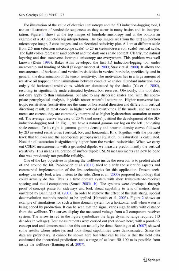
For illustration of the value of electrical anisotropy and the 3D induction-logging tool, I

use an illustration of sand/shale sequences as they occur in many basins and its interpre-

tation. Figure 1 shows at the top images of borehole anisotropy and at the bottom an

example of a 3D induction log interpretation. The top images are (from the left) an electron

microscope image, 2 core images, and an electrical resistivity plot. All are at different scale

from 2.5 mm (electron microscope scale) to 23 m (seismic/reservoir scale) vertical scale.

The light colors represent sand content and the dark ones shale content. Clearly, the natural

layering and thus transverse isotropic anisotropy are everywhere. This problem was well

known (Klein 1993). Baker Atlas developed the first 3D induction-logging tool under

mentorship and funding of Shell (Kriegshauser et al. 2000; Strack et al. 2000). It allows the

measurement of horizontal and vertical resistivities in vertical borehole, specifically, and in

general, the determination of the tensor resistivity. The motivation lies in a large amount of

resistive oil trapped in thin laminations between conductive shales. Standard induction logs

only yield horizontal resistivities, which are dominated by the shales (Yu et al. 2002),

resulting in significantly underestimated hydrocarbon reserves. Obviously, this tool does

not only apply to thin laminations, but also to any dispersed shales and, with the appro-

priate petrophysical analysis, it yields tensor water/oil saturation. Higher transverse iso-

tropic resistivities (resistivities are the same on horizontal direction and different in vertical

direction) result, in most cases, in higher vertical resistivities. If the model and measure-

ments are correct, they are commonly interpreted as higher hydrocarbon saturation or more

oil. The average reserve increase of 20 % (and more) justified the development of the 3D-

induction-logging tool. In Fig. 1, we have a natural gamma ray log on the left, indicating

shale content. To its right is gamma–gamma density and neutron density curves followed

by 2D inverted resistivities (vertical, Rv; and horizontal, Rh). Together with the porosity

track that follows and the appropriate petrophysical equation, oil saturation is calculated.

Note the oil saturation is significantly higher from the vertical resistivities. When we carry

out CSEM measurements with a grounded dipole, we measure predominantly the vertical

resistivity. This means calibration of surface dipole CSEM measurements can now be done

that was previously not possible reliably.

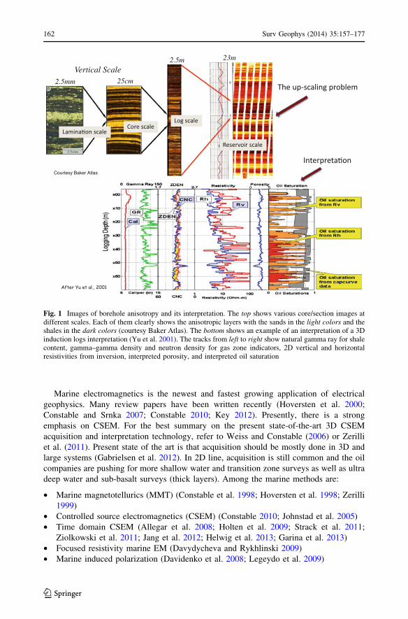
One of the key objectives in placing the wellbore inside the reservoir is to predict ahead

of and around the bit. Rabinovich et al. (2011) tried to clarify the scientific aspects and

commercial implementation of the first technologies for this application. Present tech-

nology can only look a few meters to the side. Zhou et al. (2000) proposed technology that

could actually do this. This is a time domain system with short transmitter-to-receiver

spacing and multi-components (Strack 2003a, b). The systems were developed through

proof-of-concept phase for sideways and look ahead capability to tens of meters, dem-

onstrated by Banning et al. (2007). In order to remove the effect of the drill string, special

deconvolution methods needed to be applied (Hanstein et al. 2003). Figure 2 shows an

example of simulations for such a time domain system for a horizontal well when water is

being coned by production. It can be seen that the signal varies significantly with distance

from the wellbore. The curves display the measured voltage from a 3-component receiver

system. The arrow in red in the figure symbolizes the large dynamic range required (13

decades in voltage). Test measurements were carried out (not shown here) with a proof-of-

concept tool and demonstrated that this can actually be done. Banning et al. (2007) showed

some results where sideways and look-ahead capabilities were demonstrated. Since the

data are proprietary, it cannot be shown here but what can be said is that the field data

confirmed the theoretical predictions and a range of at least 50–100 m is possible from

inside the wellbore (Banning et al. 2007).

Surv Geophys (2014) 35:157–177 161

123

Marine electromagnetics is the newest and fastest growing application of electrical

geophysics. Many review papers have been written recently (Hoversten et al. 2000;

Constable and Srnka 2007; Constable 2010; Key 2012). Presently, there is a strong

emphasis on CSEM. For the best summary on the present state-of-the-art 3D CSEM

acquisition and interpretation technology, refer to Weiss and Constable (2006) or Zerilli

et al. (2011). Present state of the art is that acquisition should be mostly done in 3D and

large systems (Gabrielsen et al. 2012). In 2D line, acquisition is still common and the oil

companies are pushing for more shallow water and transition zone surveys as well as ultra

deep water and sub-basalt surveys (thick layers). Among the marine methods are:

• Marine magnetotellurics (MMT) (Constable et al. 1998; Hoversten et al. 1998; Zerilli

1999)

• Controlled source electromagnetics (CSEM) (Constable 2010; Johnstad et al. 2005)

• Time domain CSEM (Allegar et al. 2008; Holten et al. 2009; Strack et al. 2011;

Ziolkowski et al. 2011; Jang et al. 2012; Helwig et al. 2013; Garina et al. 2013)

• Focused resistivity marine EM (Davydycheva and Rykhlinski 2009)

• Marine induced polarization (Davidenko et al. 2008; Legeydo et al. 2009)

2.5m

25cm2.5mm

Vertical Scale

23m

Courtesy Baker Atlas

Fig. 1 Images of borehole anisotropy and its interpretation. The top shows various core/section images atdifferent scales. Each of them clearly shows the anisotropic layers with the sands in the light colors and theshales in the dark colors (courtesy Baker Atlas). The bottom shows an example of an interpretation of a 3Dinduction logs interpretation (Yu et al. 2001). The tracks from left to right show natural gamma ray for shalecontent, gamma–gamma density and neutron density for gas zone indicators, 2D vertical and horizontalresistivities from inversion, interpreted porosity, and interpreted oil saturation

162 Surv Geophys (2014) 35:157–177

123

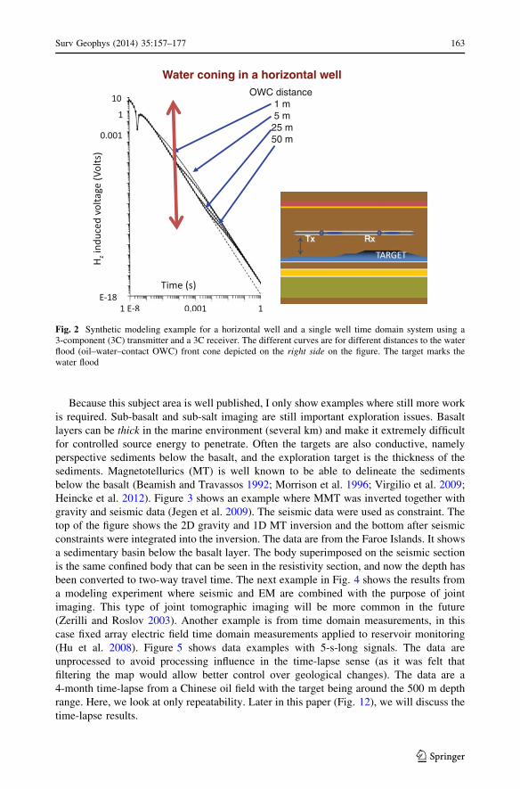
Because this subject area is well published, I only show examples where still more work

is required. Sub-basalt and sub-salt imaging are still important exploration issues. Basalt

layers can be thick in the marine environment (several km) and make it extremely difficult

for controlled source energy to penetrate. Often the targets are also conductive, namely

perspective sediments below the basalt, and the exploration target is the thickness of the

sediments. Magnetotellurics (MT) is well known to be able to delineate the sediments

below the basalt (Beamish and Travassos 1992; Morrison et al. 1996; Virgilio et al. 2009;

Heincke et al. 2012). Figure 3 shows an example where MMT was inverted together with

gravity and seismic data (Jegen et al. 2009). The seismic data were used as constraint. The

top of the figure shows the 2D gravity and 1D MT inversion and the bottom after seismic

constraints were integrated into the inversion. The data are from the Faroe Islands. It shows

a sedimentary basin below the basalt layer. The body superimposed on the seismic section

is the same confined body that can be seen in the resistivity section, and now the depth has

been converted to two-way travel time. The next example in Fig. 4 shows the results from

a modeling experiment where seismic and EM are combined with the purpose of joint

imaging. This type of joint tomographic imaging will be more common in the future

(Zerilli and Roslov 2003). Another example is from time domain measurements, in this

case fixed array electric field time domain measurements applied to reservoir monitoring

(Hu et al. 2008). Figure 5 shows data examples with 5-s-long signals. The data are

unprocessed to avoid processing influence in the time-lapse sense (as it was felt that

filtering the map would allow better control over geological changes). The data are a

4-month time-lapse from a Chinese oil field with the target being around the 500 m depth

range. Here, we look at only repeatability. Later in this paper (Fig. 12), we will discuss the

time-lapse results.

OWC distance 1 m5 m25 m50 m

Water coning in a horizontal well

Fig. 2 Synthetic modeling example for a horizontal well and a single well time domain system using a3-component (3C) transmitter and a 3C receiver. The different curves are for different distances to the waterflood (oil–water–contact OWC) front cone depicted on the right side on the figure. The target marks thewater flood

Surv Geophys (2014) 35:157–177 163

123

For land electromagnetic applications, Keller et al. 1984 summarized land CSEM and

Nekut and Spies wrote their review paper (1989) and a more general review in 1991 (Spies

and Frischknecht 1991), and the applications of EM included:

1. Sub-basalt exploration (Wilt et al. 1989; Beamish and Travassos 1992)

2. Sub-salt exploration (Hoversten et al. 2000; De Stefano et al. 2011)

3. Messy overburden (Christopherson 1991)

4. Porosity mapping (Strack et al. 1989)

5. Induced polarization applications (Sternberg and Oehler 1984)

More recent papers on sub-basalt exploration were those by Strack and Pandey (2007)

and Colombo et al. (2012). Colombo already derived different products from the data,

namely adjustments to seismic velocities and thus improved seismic images.

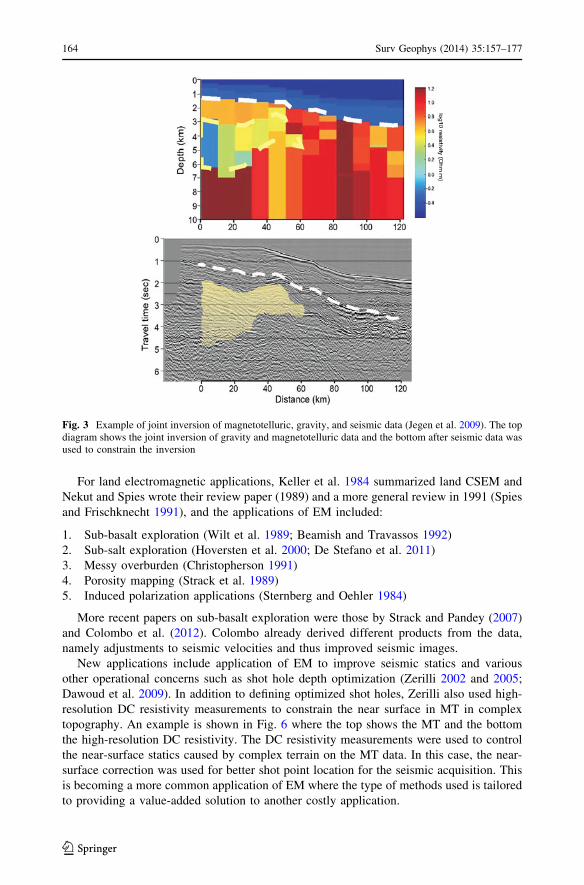
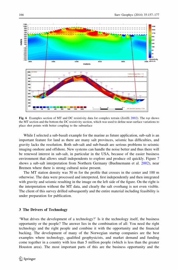
New applications include application of EM to improve seismic statics and various

other operational concerns such as shot hole depth optimization (Zerilli 2002 and 2005;

Dawoud et al. 2009). In addition to defining optimized shot holes, Zerilli also used high-

resolution DC resistivity measurements to constrain the near surface in MT in complex

topography. An example is shown in Fig. 6 where the top shows the MT and the bottom

the high-resolution DC resistivity. The DC resistivity measurements were used to control

the near-surface statics caused by complex terrain on the MT data. In this case, the near-

surface correction was used for better shot point location for the seismic acquisition. This

is becoming a more common application of EM where the type of methods used is tailored

to providing a value-added solution to another costly application.

Fig. 3 Example of joint inversion of magnetotelluric, gravity, and seismic data (Jegen et al. 2009). The topdiagram shows the joint inversion of gravity and magnetotelluric data and the bottom after seismic data wasused to constrain the inversion

164 Surv Geophys (2014) 35:157–177

123

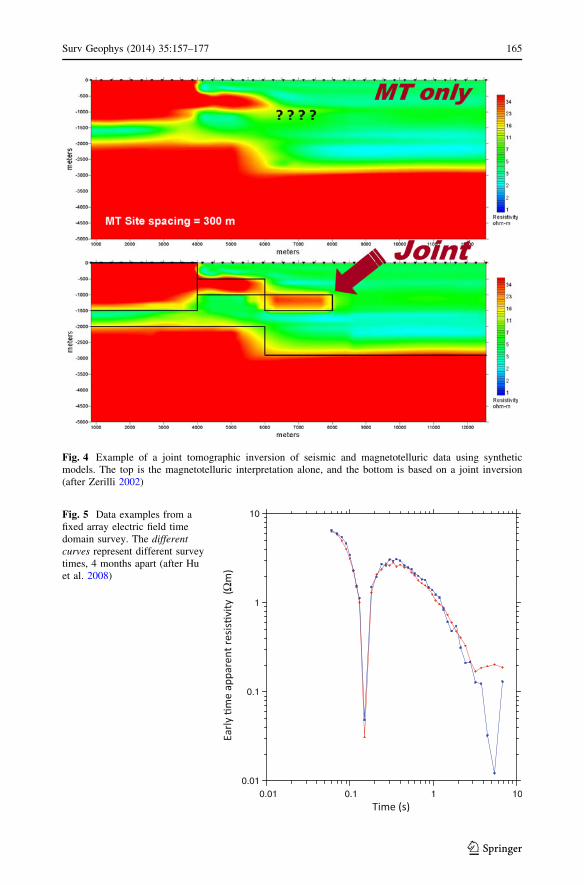
Fig. 4 Example of a joint tomographic inversion of seismic and magnetotelluric data using syntheticmodels. The top is the magnetotelluric interpretation alone, and the bottom is based on a joint inversion(after Zerilli 2002)

Fig. 5 Data examples from afixed array electric field timedomain survey. The differentcurves represent different surveytimes, 4 months apart (after Huet al. 2008)

Surv Geophys (2014) 35:157–177 165

123

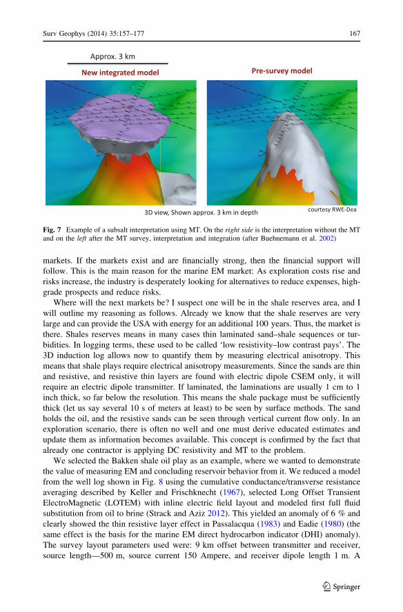
While I selected a sub-basalt example for the marine as future application, sub-salt is an

important feature for land as there are many salt provinces, seismic has difficulties, and

gravity lacks the resolution. Both sub-salt and sub-basalt are serious problems to seismic

imaging onshore and offshore. New systems can handle the noise better and thus there will

be renewed interest in sub-salt, in particular in the USA, because of the easier business

environment that allows small independents to explore and produce oil quickly. Figure 7

shows a sub-salt interpretation from Northern Germany (Buehnemann et al. 2002), near

Bremen where there is strong cultural noise present.

The MT station density was 50 m for the profile that crosses in the center and 100 m

otherwise. The data were processed and interpreted, first independently and then integrated

with gravity and seismic resulting in the image on the left side of the figure. On the right is

the interpretation without the MT data, and clearly the salt overhang is not even visible.

The client of this survey drilled subsequently and the entire material including feasibility is

under preparation for publication.

3 The Drivers of Technology

‘What drives the development of a technology?’ Is it the technology itself, the business

opportunity or the people? The answer lies in the combination of all: You need the right

technology and the right people and combine it with the opportunity and the financial

backing. The development of many of the Norwegian startup companies are the best

examples where technology, qualified geophysicists, and market demand and funding

come together in a country with less than 5 million people (which is less than the greater

Houston area). The most important parts of this are the business opportunity and the

Fig. 6 Examples section of MT and DC resistivity data for complex terrain (Zerilli 2002). The top showsthe MT section and the bottom the DC resistivity section, which was used to define near-surface variations toplace shot points with better coupling to the subsurface

166 Surv Geophys (2014) 35:157–177

123

markets. If the markets exist and are financially strong, then the financial support will

follow. This is the main reason for the marine EM market: As exploration costs rise and

risks increase, the industry is desperately looking for alternatives to reduce expenses, high-

grade prospects and reduce risks.

Where will the next markets be? I suspect one will be in the shale reserves area, and I

will outline my reasoning as follows. Already we know that the shale reserves are very

large and can provide the USA with energy for an additional 100 years. Thus, the market is

there. Shales reserves means in many cases thin laminated sand–shale sequences or tur-

bidities. In logging terms, these used to be called ‘low resistivity–low contrast pays’. The

3D induction log allows now to quantify them by measuring electrical anisotropy. This

means that shale plays require electrical anisotropy measurements. Since the sands are thin

and resistive, and resistive thin layers are found with electric dipole CSEM only, it will

require an electric dipole transmitter. If laminated, the laminations are usually 1 cm to 1

inch thick, so far below the resolution. This means the shale package must be sufficiently

thick (let us say several 10 s of meters at least) to be seen by surface methods. The sand

holds the oil, and the resistive sands can be seen through vertical current flow only. In an

exploration scenario, there is often no well and one must derive educated estimates and

update them as information becomes available. This concept is confirmed by the fact that

already one contractor is applying DC resistivity and MT to the problem.

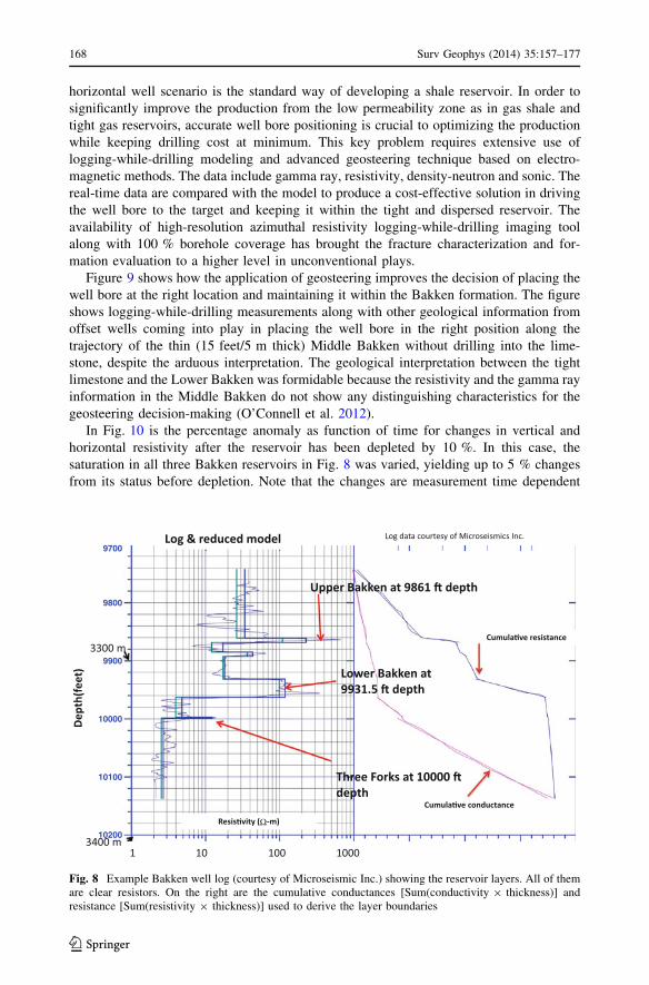
We selected the Bakken shale oil play as an example, where we wanted to demonstrate

the value of measuring EM and concluding reservoir behavior from it. We reduced a model

from the well log shown in Fig. 8 using the cumulative conductance/transverse resistance

averaging described by Keller and Frischknecht (1967), selected Long Offset Transient

ElectroMagnetic (LOTEM) with inline electric field layout and modeled first full fluid

substitution from oil to brine (Strack and Aziz 2012). This yielded an anomaly of 6 % and

clearly showed the thin resistive layer effect in Passalacqua (1983) and Eadie (1980) (the

same effect is the basis for the marine EM direct hydrocarbon indicator (DHI) anomaly).

The survey layout parameters used were: 9 km offset between transmitter and receiver,

source length—500 m, source current 150 Ampere, and receiver dipole length 1 m. A

Fig. 7 Example of a subsalt interpretation using MT. On the right side is the interpretation without the MTand on the left after the MT survey, interpretation and integration (after Buehnemann et al. 2002)

Surv Geophys (2014) 35:157–177 167

123

horizontal well scenario is the standard way of developing a shale reservoir. In order to

significantly improve the production from the low permeability zone as in gas shale and

tight gas reservoirs, accurate well bore positioning is crucial to optimizing the production

while keeping drilling cost at minimum. This key problem requires extensive use of

logging-while-drilling modeling and advanced geosteering technique based on electro-

magnetic methods. The data include gamma ray, resistivity, density-neutron and sonic. The

real-time data are compared with the model to produce a cost-effective solution in driving

the well bore to the target and keeping it within the tight and dispersed reservoir. The

availability of high-resolution azimuthal resistivity logging-while-drilling imaging tool

along with 100 % borehole coverage has brought the fracture characterization and for-

mation evaluation to a higher level in unconventional plays.

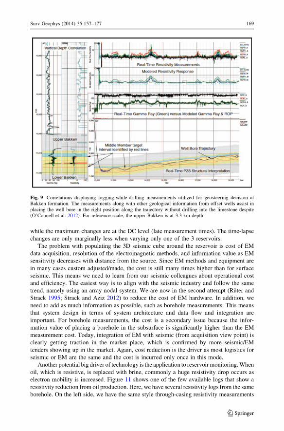
Figure 9 shows how the application of geosteering improves the decision of placing the

well bore at the right location and maintaining it within the Bakken formation. The figure

shows logging-while-drilling measurements along with other geological information from

offset wells coming into play in placing the well bore in the right position along the

trajectory of the thin (15 feet/5 m thick) Middle Bakken without drilling into the lime-

stone, despite the arduous interpretation. The geological interpretation between the tight

limestone and the Lower Bakken was formidable because the resistivity and the gamma ray

information in the Middle Bakken do not show any distinguishing characteristics for the

geosteering decision-making (O’Connell et al. 2012).

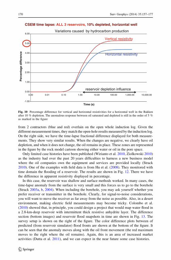
In Fig. 10 is the percentage anomaly as function of time for changes in vertical and

horizontal resistivity after the reservoir has been depleted by 10 %. In this case, the

saturation in all three Bakken reservoirs in Fig. 8 was varied, yielding up to 5 % changes

from its status before depletion. Note that the changes are measurement time dependent

Fig. 8 Example Bakken well log (courtesy of Microseismic Inc.) showing the reservoir layers. All of themare clear resistors. On the right are the cumulative conductances [Sum(conductivity 9 thickness)] andresistance [Sum(resistivity 9 thickness)] used to derive the layer boundaries

168 Surv Geophys (2014) 35:157–177

123

while the maximum changes are at the DC level (late measurement times). The time-lapse

changes are only marginally less when varying only one of the 3 reservoirs.

The problem with populating the 3D seismic cube around the reservoir is cost of EM

data acquisition, resolution of the electromagnetic methods, and information value as EM

sensitivity decreases with distance from the source. Since EM methods and equipment are

in many cases custom adjusted/made, the cost is still many times higher than for surface

seismic. This means we need to learn from our seismic colleagues about operational cost

and efficiency. The easiest way is to align with the seismic industry and follow the same

trend, namely using an array nodal system. We are now in the second attempt (Ruter and

Strack 1995; Strack and Aziz 2012) to reduce the cost of EM hardware. In addition, we

need to add as much information as possible, such as borehole measurements. This means

that system design in terms of system architecture and data flow and integration are

important. For borehole measurements, the cost is a secondary issue because the infor-

mation value of placing a borehole in the subsurface is significantly higher than the EM

measurement cost. Today, integration of EM with seismic (from acquisition view point) is

clearly getting traction in the market place, which is confirmed by more seismic/EM

tenders showing up in the market. Again, cost reduction is the driver as most logistics for

seismic or EM are the same and the cost is incurred only once in this mode.

Another potential big driver of technology is the application to reservoir monitoring. When

oil, which is resistive, is replaced with brine, commonly a huge resistivity drop occurs as

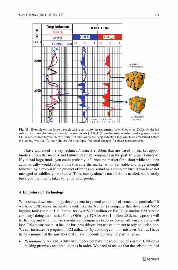
electron mobility is increased. Figure 11 shows one of the few available logs that show a

resistivity reduction from oil production. Here, we have several resistivity logs from the same

borehole. On the left side, we have the same style through-casing resistivity measurements

Fig. 9 Correlations displaying logging-while-drilling measurements utilized for geosteering decision atBakken formation. The measurements along with other geological information from offset wells assist inplacing the well bore in the right position along the trajectory without drilling into the limestone despite(O’Connell et al. 2012). For reference scale, the upper Bakken is at 3.3 km depth

Surv Geophys (2014) 35:157–177 169

123

from 2 contractors (blue and red) overlain on the open whole induction log. Given the

different measurement times, they match the open-hole results measured by the induction log.

On the right side, we have the time-lapse fractional difference displayed for both measure-

ments. They show very similar results. When the changes are negative, we clearly have oil

depletion, and when it does not change, the oil remains in place. These zones are represented

in the figure by the rock model cartoon showing either water or oil in the pore space.

Only limited case histories have been published (Wirianto et al. 2010, Ziolkowski 2010)

as the industry had over the past 20 years difficulties to harness a new business model

where the oil companies own the equipment and services are provided locally (Strack

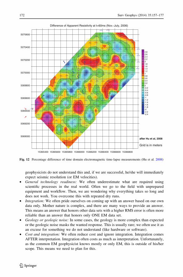
2010). One of the examples with field data is from Hu et al. (2008). They monitored with

time domain the flooding of a reservoir. The results are shown in Fig. 12. There we have

the difference in apparent resistivity displayed in percentage.

In this case, the reservoir was shallow and surface methods worked. In many cases, the

time-lapse anomaly from the surface is very small and this forces us to go to the borehole

(Strack 2003a, b, 2004). When including the borehole, you may ask yourself whether you

prefer receiver or transmitter in the borehole. Clearly, for signal-to-noise considerations,

you will want to move the receiver as far away from the noise as possible. Also, in a desert

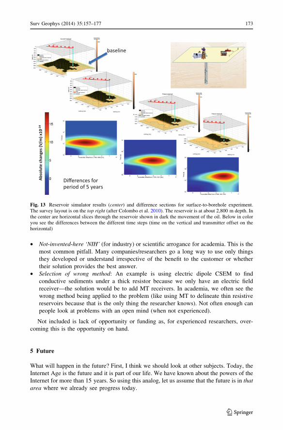
environment, making electric field measurements may become tricky. Colombo et al.

(2010) showed that, in principle, you could design a project that would map water flood in

a 2.8-km-deep reservoir with intermittent thick resistive anhydrite layer. The difference

section (bottom images) and reservoir flood snapshots in time are shown in Fig. 13. The

survey setup is shown on the right of the figure. The color difference plots between of

predicted (from reservoir simulator) flood fronts are shown at the bottom of the figure. It

can be seen that the anomaly moves along with the oil front movement (the red maximum

moves to the right where the oil remains). Again, this is an area of increased market

activities (Dutta et al. 2011), and we can expect in the near future some case histories.

-1.00

0.00

1.00

2.00

3.00

4.00

5.00

6.00

0.00 0.01 0.10 1.00 10.00 100.00 1,000.00 10,000.00

CSEM time lapse: ALL 3 reservoirs, 10% depleted, horizontal well

Time (s)

Per

cen

tag

e d

iffe

ren

ce

Vertical resistivity

Horizontal resistivity

Variations caused by hydrocarbon production

reservoir depletion influence

Fig. 10 Percentage difference for vertical and horizontal resistivities for a horizontal well in the Bakkenafter 10 % depletion. The anomalous response between oil saturated and depleted is still in the order of 5 %as marked in the figure

170 Surv Geophys (2014) 35:157–177

123

I have addressed the key technical/business enablers that are based on market oppor-

tunities. From the success and failures of small companies in the past 15 years, I observe:

If you had large funds, you could probably influence the market for a short while and then

automatically would come a bust (because the market is not yet stable and large enough)

followed by a revival if the product offerings are sound or a complete bust if you have not

managed to stabilize your product. Thus, money alone is not all that is needed, but it surely

buys you the time it takes to refine your product.

4 Inhibitors of Technology

What slows down technology development in general and proof-of-concept in particular? If

we have ONE super successful event, like the Numar (a company that developed NMR

logging tools) sale to Halliburton for over $300 million or EMGS (a marine EM service

company) doing their Initial Public Offering (IPO) for over 1 billion US $, many people will

try to copy and will mobilize scientists and engineers to do so. Some will win and some will

lose. This means we must include business drivers, but use caution not to rely on luck alone.

We can increase the progress of EM utilization by avoiding common mistakes. Below, I have

listed a number of the mistakes that I have encountered over the past 30 years.

• Resolution: Since EM is diffusive, it does not have the resolution of seismic. Caution in

making promises and prediction is in order. We need to realize that the seismic trained

Fig. 11 Example of time lapse through-casing resistivity measurements (after Zhou et al. 2002). On the leftside are the through-casing resistivity measurements [TCR_L (through-casing resistivity—long spaced) andCHFR (cased hole formation resistivity)] in addition to the deep induction log, which was measured beforethe sassing was set. To the right are the time-lapse fractional changes for these measurements

Surv Geophys (2014) 35:157–177 171

123

geophysicists do not understand this and, if we are successful, he/she will immediately

expect seismic resolution (or EM velocities).

• General technology readiness: We often underestimate what are required using

scientific processes in the real world. Often we go to the field with unprepared

equipment and workflow. Then, we are wondering why everything takes so long and

does not work. You overcome this with repeated dry runs.

• Integration: We often pride ourselves on coming up with an answer based on our own

data only. Mother nature is complex, and there are many ways to provide an answer.

This means an answer that honors other data sets with a higher RMS error is often more

reliable than an answer that honors only ONE EM data set.

• Geology or geologic noise: In some cases, the geology is more complex than expected

or the geologic noise masks the wanted response. This is usually rare; we often use it as

an excuse for something we do not understand (like hardware or software).

• Cost and integration: We often reduce cost and ignore integration. Integration comes

AFTER interpretation. Integration often costs as much as interpretation. Unfortunately,

as the common EM geophysicist knows mostly or only EM, this is outside of his/her

scope. This means we need to plan for this.

15365400 15365600 15365800 15366000 15366200 15366400 15366600 15366800

Difference of Apparent Resistivity at t=60ms (Nov.-July, 2006)

5069000

5069200

5069400

5069600

5069800

5070000

5070200

5070400

5070600

95714

95724

95725

95726

95735

95736

95737

95738

95739

95747

95748

95749

95750

95751

95752

95753

95759

95761

95763

95765

95766

95767

95768

95769

95771

95772

95775

95776

95777

95778

95779

95781

95782

95783

95784

95785

95786

95787

95788

95789

95791

95793

95797

95798

95799

95900

95901

95902

95903

95904

95909

95910

95911

95912

95913

95915

95916

95917

95918

95919

95922 9592395924

95931

95935 95938 95939

95945

95958 95959 95960

95961

95962

951204

951207

951208

951212

951213

951214

951215

951216

951218 951221

951222

951228

951229

951231

951232

951233

951237

951240

951241

951243

951244

951245

951246

951248

951249

951254

951255

951256

951257

951269 951270951271

951272

951276 951277

951284

951622 951623

951629 951630

J448

-2.4-2.2-2-1.8-1.6-1.4-1.2-1-0.8-0.6-0.4-0.200.20.40.60.811.21.41.61.822.22.42.62.8

95760

95762

95764

95770

95780

95790

95792

95794

95795

95796

95926 95927 95928 95929 95930

95934 95936 95937

95943 95944 95946 95947

95953

95968 95969

95977 95978

95985

951200

951201

951202

951203

951205

951206

951209

951210

951211 951217

951225

951226

951230

951235

951236

951238

951239

951247

951250951251

951252

951267 951268

951278 951279

951286

after Hu et al, 2008

Grid is in meters

Fig. 12 Percentage difference of time domain electromagnetic time-lapse measurements (Hu et al. 2008)

172 Surv Geophys (2014) 35:157–177

123

• Not-invented-here ‘NIH’ (for industry) or scientific arrogance for academia. This is the

most common pitfall. Many companies/researchers go a long way to use only things

they developed or understand irrespective of the benefit to the customer or whether

their solution provides the best answer.

• Selection of wrong method: An example is using electric dipole CSEM to find

conductive sediments under a thick resistor because we only have an electric field

receiver—the solution would be to add MT receivers. In academia, we often see the

wrong method being applied to the problem (like using MT to delineate thin resistive

reservoirs because that is the only thing the researcher knows). Not often enough can

people look at problems with an open mind (when not experienced).

Not included is lack of opportunity or funding as, for experienced researchers, over-

coming this is the opportunity on hand.

5 Future

What will happen in the future? First, I think we should look at other subjects. Today, the

Internet Age is the future and it is part of our life. We have known about the powers of the

Internet for more than 15 years. So using this analog, let us assume that the future is in that

area where we already see progress today.

Fig. 13 Reservoir simulator results (center) and difference sections for surface-to-borehole experiment.The survey layout is on the top right (after Colombo et al. 2010). The reservoir is at about 2,800 m depth. Inthe center are horizontal slices through the reservoir shown in dark the movement of the oil. Below in coloryou see the differences between the different time steps (time on the vertical and transmitter offset on thehorizontal)

Surv Geophys (2014) 35:157–177 173

123

• Clearly hardware cost is coming down and will come down more. The past 2 years

reduced EM system cost by 60 %. Another 50 % and more is needed to make EM

attractive to seismic geophysicists. The driver will be that we need more data, which

means cost per data point must come down but total hardware expenditure will go up.

• Denser measurements and higher data redundancy. As with seismic, spatial sampling

must go much higher than the Nyquist frequency. It does not help to look with MT for

50-m intrusions with 1-km station spacing (this means we are still under-sampling).

Higher spatially oversampled measurements will be the standard.

• Operational decisions will drive EM applications, mainly to improve seismic

acquisition (static, complex structure and topography and shot hole optimization),

but also for site investigations, environmental certifications, etc. This will be a big

growth area as it immediately adds to the bottom line.

• Shale applications: Slowly, even the seismic geophysicists in oil companies are

realizing that EM could contribute to solving their problem. A pilot demonstration is

still outstanding, but I have no doubt this will happen in the next 12–24 months. The

potential benefits are simply too big.

• Reservoir monitoring applications: Slowly, we see the first case histories and some oil

companies are pushing this openly. The industry will adopt better business models to

match this, and the technology will be provided as it is already there.

• In the borehole, we will see even more emphasis on geosteering. The more information

we have close to drilling, the less formation evaluation we have to do afterward.

• The marine environment will further mature, but we will see a trend to services integration

as has happened everywhere else. 3D acquisition will be the standard, and full integration

of ALL EM methods will be the normal product (not just CSEM or electric fields).

• The patent space will become more diverse in terms of methods. Geographic loop holes

will become less important as violators will be caught in different jurisdictions as

globalization progresses.

• There will be more integration with seismics forthcoming shortly as some progress

happened since 1990 (Strack and Vozoff 1996). We still do not have routine joint

seismic/EM acquisition or processing and only limited proposals for integrated

interpretation. Given the increased request for this (Harris et al. 2009; Gao et al. 2011;

Ellis et al. 2011), we can only hope to see more integration in the next few years.

Overall, the potential for a great career in electrical geophysics is there as long as we

can follow the guidance of the problem on hand and strive for the best solution.

Acknowledgments I would like to acknowledge the support of KMS Technologies, Geokinetics, RWE-Dea, Shell, BP, Chevron, ConocoPhillips, and Baker Hughes. In particular, I appreciate the support from A.A. Aziz, A. Zerilli, K. Vozoff, T. Hanstein, L. Thomsen, C. Stoyer, S. Dasgupta, and W. Hu.

References

Allegar NA, Strack KM, Mittet R, Petrov A (2008) Marine time domain CSEM—the first two years ofexperience. 70th Conference & exhibition, European Association Geoscientists & Engineers, Rome,Italy, abstract vol

Banning EJ, Hagiwara T, Ostermeier RM (2007) Imaging of a subsurface conductivity distribution using atime-domain electromagnetic borehole-conveyed logging tool. SEG technical program expandedabstracts, 26, 648

Beamish D, Travassos JM (1992) Magnetotelluric of Basalt-covered sediments. First Break 10:345–357Blau W (1933) Methods and apparatus for geophysical exploration. US Patent 1,911,137

174 Surv Geophys (2014) 35:157–177

123

Buehnemann J, Henke CH, Mueller C, Krieger MH, Zerilli A, Strack KM (2002) Bringing complex saltstructures into focus—a novel integrated approach: SEG technical program expanded abstracts,pp 446–449

Christopherson KR (1991) Applications of magnetotellurics to petroleum exploration in Papua New Guinea:a model for frontier areas. Lead Edge 10:21–27

Colombo D, Dasgupta S, Strack KM, Yu G (2010) Feasibility study of surface-to-borehole CSEM for oil-water fluid substitution in Ghawar field, Saudi Arabia: Geo 2010, poster

Colombo D, Keho T, McNeice G (2012) Integrated seismic-electromagnetic workflow for sub-basaltexploration in northwest Saudi Arabia. Lead Edge 31:42–53

Constable S (2010) Ten years of marine CSEM for hydrocarbon exploration. Geophysics 75:75A67–75A81Constable S, Srnka LJ (2007) An introduction to marine controlled-source electromagnetic methods for

hydrocarbon exploration. Geophysics 72:WA3–WA12Constable S, Orange A, Hoversten GM, Morrison HF (1998) Marine for petroleum exploration, Part 1: a sea-

floor instrument system. Geophysics 63:816–825Davidenko Y, Ivanov S, Kudryavceca E, Legeydo P, Veeken PCH (2008) Geoelectric surveying, a useful

tool for hydrocarbon exploration. EAEG annual meeting expanded abstract vol, Roma, p 301Davydycheva S, Rykhlinski N (2009) Focused-source EM survey versus time-domain and frequency-

domain CSEM. Lead Edge 28:944–949Dawoud M, Hallinan S, Herrmann R, van Kleef F (2009) Near-surface electromagnetic surveying. Oil Field

Rev 21:20–25De Stefano M, Andreasi FG, Virgilio M, Snyder F (2011) Multiple-domain, simultaneous joint inversion of

geophysical data with application to subsalt imaging. Geophysics 76:R69–R80Dutta SM, Reiderman A, Rabinovich MB, Schoonover LG (2011) Novel transient electromagnetic Borehole

system for reservoir monitoring. SPE annual technical conference and exhibition, Denver, Colorado,USA

Eadie T (1980) Detection of hydrocarbon accumulations by surface electrical methods—feasibility study.M. S. Thesis, University of Toronto

Eidesmo T, Ellingsrud S, MacGregor LM, Constable S, Sinha MS, Johansen S, Kong FN, Westerdahl H(2002) Sea bed logging (SBL), a new method for remote and direct identification of hydrocarbon filledlayers in deep-water areas. First Break 20:144–152

Ellis M, Ruiz F, Nanduri S, Keirstead R, Azizov I, Frenkel M, MacGregor L (2011) Importance ofanisotropic rock physics modelling in integrated seismic and CSEM interpretation. First Break29:87–95

Gabrielsen PT, Shantsev DV, Fanavoll S (2012) 3D CSEM for hydrocarbon exploration in the Barents Sea.EAGE 5th Saint Petersburg conference & exhibition, April 2012, paper C002

Gao G, Abubaker A, Habashy TM (2011) Inversion of porosity and fluid saturation from joint electro-magnetic and elastic full-waveform data. SEG technical program expanded abstracts, pp 660–665

Garina S, Ivanov S, Kudryavceva E, Legeydo P, Veeken P, Vladimirov V (2013) Simultaneous EM and IPinversion using relaxation time constraints. First Break 31:69–72

Gruner Schlumberger A (1982) The Schlumberger adventure. Arco Publish, New YorkHanstein T, Rueter H, Strack KM (2003) LWD induction deconvolution methods. US Patent 6,891,376Harris PE, Du L, MacGregor L, Olsen W, Shu R, Cooper R (2009) Joint interpretation of seismic and CSEM

data using well log constraints: and example from Luva Field. First Break 27:73–81Heincke B, Moorkamp M, Jegen M (2012) Joint inversion of 3-D seismic. Gravimetric and magnetotelluric

data for sub-basalt imaging in the Faroe-Shetland Basin, AGU Fall meeting posterHelwig SL, El Kaffas AW, Holten T, Frafjord O, Eide K (2013) Vertical dipole CSEM: technology

advances and results from Snohvit field. First Break 31:63–68Hesthammer J, Fanavoll S, Stefatos A, Danielsen JE, Boulaenko M (2010) CSEM performance in light of

well results. Lead Edge 29:34–41Hesthammer J, Stefatos A, Sperrevik S (2012) CSEM efficiency—evaluation of recent drilling results. First

Break 30:47–55Holten T, Flekkoy EG, Singer B, Blixt EM, Hanssen A, Maloy KJ (2009) Vertical source, vertical receiver,

electromagnetic technique for offshore hydrocarbon exploration. First Break 27:89–93Hoversten GM, Morrison HF, Constable S (1998) Marine magnetotellurics for petroleum exploration, Part

2: numerical analysis of subsalt resolution. Geophysics 63:826–840Hoversten GM, Constable S, Morrison HF (2000) Marine magnetotellurics for base-of-salt mapping: Gulf of

Mexico field-test at the Gemini structure. Geophysics 65:1476–1488Hu W, Yan L, Su Z, Zheng R, Strack KM (2008) Array TEM sounding and application for reservoir

monitoring. SEG technical program expanded abstracts, pp 634–638

Surv Geophys (2014) 35:157–177 175

123

Jang H, Jang H, Lee K-H, Kim J (2012) A transient EM method with vertical transmitter and receiver foroffshore hydrocarbon exploration. SEG technical program expanded abstracts, pp 1–5

Jegen M, Hobbs RW, Tarits P, Chave A (2009) Joint inversion of marine magnetotelluric and gravity dataincorporating seismic constraints—preliminary results of sub-basalt imaging off the Faroe Shelf. EarthPlanet Sci Lett 282:47–55

Johnstad SE, Farrelly BA, Ringstad C (2005) EM seabed logging on the Troll field. 67th Conference &exhibition, European Association Geoscientists & Engineers, Madrid, Spain, abstract vol

Keller GV, Frischknecht FC (1967) Electrical methods in geophysical prospecting. Pergamon Press, NewYork

Keller GV, Pritchard JI, Jacobson JJ, Harthill N (1984) Mega source time-domain electromagnetic soundingmethods. Geophysics 49:993–1009

Key K (2012) Marine electromagnetic studies of the seafloor resources and tectonics. Surv Geophys33:135–137

Klein JD (1993) Induction log anisotropy offer a means of detection of very thinly bedded corrections. LogAnalyst 34:18–27

Kriegshauser B, Fanini O, Forgang S, Mollison RA, Yu L, Gupta PK, Koelman JMV, van Popta J (2000)Increased oil-in-place in low-resistivity reservoirs from multicomponent induction log data. SPWLAannual meeting transactions vol, Paper A

Kumar D, Hoversten GM (2012) Geophysical model response in shale gas. Geohorizons 17:32–37Legeydo P, Veeken PCH, Petserev I, Davidenko Y, Kudryyaceca E, Ivanov S (2009) Geoelectric analysis

based on quantitative separation between Electromagnetic and induced polarization field response.EAGE annual meeting expanded abstract vol, Amsterdam, P078

Luthi SM (2001) Geological well logs—their use in reservoir modeling. Springer, Berlin, p 373Morrison HF, Shoham Y, Hoversten GM, Torres-Verdin C (1996) Electromagnetic mapping of electrical

conductivity beneath the Columbia basalt. Geophys Prospect 44:935–961Nabighian MN, Macnae JC (2005) Electrical and EM methods 1980–2005. Lead Edge 24:S42–S45Nekut AG, Spies BR (1989) Petroleum exploration using controlled-source electromagnetic methods. Proc

IEEE 77:338–362O’Connell K, Skaria D, Wheeler A, Rennie A (2012) Geosteering Improves Bakken Results. Am Oil Gas

Rep 55Passalacqua H (1983) Electromagnetic fields due to a thin resistive layer. Geophys Prospect 31:945–976Rabinovich M, Le F, Lofts J, Martakov S (2011) Deep? How deep and what? The vagaries and myths of

‘Look around’ deep-resistivity measurements while drilling. SPWLA transactions, paper NNNRuter H, Strack K-M (1995) Method of processing transient electromagnetic measurements in geophysical

analysis. US Patent 5,467,018Schilowsky K (1913) Verfahren und Vorrichtung zum Nachweis unterirdischer Erzlager oder von Grund-

wasser mittels elektrischer Schwingungen: German Patent 322,040Sheard SN, Ritchie TJ, Christopherson KR, Brand E (2005) Mining, environmental, petroleum and engi-

neering industry applications of electromagnetics techniques in geophysics. Surv Geophys 26:653–669Spies BR (1983) Recent developments in the use of surface electrical methods for oil and gas exploration in

the Soviet Union. Geophysics 48:1102–1112Spies BR, Frischknecht FC (1991) Electromagnetic sounding. In: Nabighian MN (ed) Electromagnetic

methods in applied geophysics-applications: SEG invest. Geophysics ser # 3, Soc Expl Geophys, SEGinvest Geophys ser #3, pp 285–426

Srnka LJ, Carazzone JJ, Ephron MS, Eriksen EA (2006) Remote reservoir resistivity mapping. Lead Edge25:972–975

Sternberg BK, Oehler DZ (1984) Electrical methods for hydrocarbon exploration I. Induced polarization(INDEPTH) method: unconventional methods in exploration for petroleum and natural gas III.,Southern Methodist Univ. Press, University Park, pp 188–201

Strack K-M (2003a) Integrated borehole system for reservoir detection and monitoring. US Patent 6,541,975Strack K-M (2003b) Integrated borehole system for reservoir detection and monitoring. US Patent

6,670,813. Continuation of 6,541,975Strack KM (2004) Combine surface and borehole integrated electromagnetic apparatus to determine res-

ervoir fluid properties. US Patent 6,739,165Strack KM (2010) Advances in electromagnetics for reservoir monitoring. Geohorizons 15–18Strack KM, Aziz AA (2012) Full field array electromagnetics: a tool kit for 3D applications to uncon-

ventional resources. GSH spring symposium honoring R.E. Sheriff, April 11–12, 2012 (see GSHwebsite)

Strack K-M, Pandey PB (2007) Exploration with controlled-source electromagnetics under basalt covers inIndia. Lead Edge 26:360–363

176 Surv Geophys (2014) 35:157–177

123

Strack KM, Vozoff K (1996) Integrating long-offset transient electromagnetics (LOTEM) with seismics inan exploration environment. Geophys Prospect 44:99–101

Strack K-M, Hanstein T, Lebrocq K, Moss DC, Petry HG, Vozoff K, Wolfgram PA (1989) Case histories ofLOTEM surveys in hydrocarbon prospective areas. First Break 7:467–477

Strack K-M, Fanini ON, Mezzatesta AG, Tabarovsky LA (1998) Recent advances in Borehole resistivitylogging. Presented at annual ASEG conference, Hobart, Australia

Strack K-M, Tabarovsky LA, Beard DB, van der Horst M (2000) Determining electrical conductivity of alaminated earth formation using induction logging. US Patent 6,147,496

Strack KM, Hanstein T, Stoyer CH, Thomsen L (2011) Time domain controlled source electromagnetics forhydrocarbon applications. In: Petrovsky E, Herrero-Bervera E; Harinarayana T, Ivers D (eds) Theearth’s magnetic interior, IAGA special Sopron book series, Springer, pp 101–115

Virgilio M, Masnaghetti L, Clementi M, Watts MD (2009) Simultaneous joint inversion of MMT andseismic data for sub-basalt exploration on the Atlantic margin, Norway. 71st EAGE conference andexhibition, P258

Weiss CJ, Constable S (2006) Mapping thin resistors and hydrocarbon with marine EM methods, Part II—modeling and analysis in 3D. Geophysics 71:321–332

Wenner F (1912) The four-terminal conductor and the Thomson bridge. US Bureau Stand Bull 8:559–610Wilt MJ, Morrison HF, Lee KH, Goldstein NE (1989) Electromagnetic sounding in the Columbia Basin,

Yakima, Washington. Geophysics 54:952–961Wirianto M, Mulder WA, Slob EC (2010) A feasibility study of land CSEM reservoir monitoring in a

complex 3-D model. Geophys J Int 1:602–606Yu L, Fanini ON, Kriegshaeuser BF, Koelman JMV, van Popta J (2001) Enhanced evaluation of low-

resistivity reservoirs using new multicomponent induction log data. Petrophysics 42:611–623Yu G, Strack KM, Tulinius H, Porbergsottir IM, Adam L, Hu ZZ, He ZX (2010) Integrated MT/Gravity

geothermal exploration in Hungary: A success story, 21st ASEG Conference and Exhibition, SydneyZerilli A (1999) Application of marine Magnetotelluric to commercial exploration—cases from the Med-

iterranean and the Gulf of Mexico: European Association of Geophysical Engineers, 61st meeting andtechnical exhibition, Helsinki, Finland, 7–11 June

Zerilli A (2002) Integrated imaging ads value to complex stricture exploration: Soc Expl Geophys annualmeeting, workshops (see www.SEG.org for audio recording and www.kmstechnologies.com)

Zerilli A (2005) Using non-seismic geophysics to enhance seismic in complex shallow regimes. EAGEworkshop W6, EAGE annual conference & exhibition

Zerilli A, Roslov Y (2003) A new approach to complex structures exploration improves resolution andreduces risk. SEG/EAGO/EAGE/PAEH international geophysical conference & exhibition, MoscowRussia, 1–4 September

Zerilli A, Labruzzo T, Buonora MP, Abubakar A (2011) Joint inversion of marine CSEM and MT data usinga ‘‘structure’’ based approach. SEG technical program expanded abstracts, pp 604–608

Zhou Q, Gregory D, Chen C, Chew WC (2000) Investigation on electromagnetic measurement ahead ofdrill-bit. IEEE international geoscience and remote sensing symposium

Zhou Q, Julander D, Penley L (2002) Experiences with cased hole resistivity logging for reservoir moni-toring. SPWLA 43rd annual logging symposium, Paper X

Ziolkowski A, Parr R, Wright D, Nockles V, Limond C, Morris E, Linfoot J (2010) Multi-transient magneticrepeatability experiment over the North Sea Harding field. Geophys Prospect 58:1159–1176

Ziolkowski A, Wright D, Mattsson J (2011) Comparison of PRBS and square wave transient CSEM dataover Peon Gas Discovery, Norway. SEG technical program expanded abstracts, pp 583–588

Surv Geophys (2014) 35:157–177 177

123