Fuzzy Geodesics and Consistent Sparse …funk/fuzzy_geodesics.pdfFuzzy Geodesics and Consistent Sparse Correspondences ... A geodesic is a parameterized curve ... Fuzzy Geodesics and

Eurographics Symposium on Geometry Processing 2010Olga Sorkine and Bruno Lévy(Guest Editors)

Volume 29 (2010), Number 5

Fuzzy Geodesics and Consistent Sparse Correspondences

For Deformable Shapes

Jian Sun and Xiaobai Chen and Thomas A. Funkhouser

Princeton University, Princeton NJ, 08544 USA

Abstract

A geodesic is a parameterized curve on a Riemannian manifold governed by a second order partial differential

equation. Geodesics are notoriously unstable: small perturbations of the underlying manifold may lead to dra-

matic changes of the course of a geodesic. Such instability makes it difficult to use geodesics in many applications,

in particular in the world of discrete geometry. In this paper, we consider a geodesic as the indicator function of

the set of the points on the geodesic. From this perspective, we present a new concept called fuzzy geodesics andshow that fuzzy geodesics are stable with respect to the Gromov-Hausdorff distance. Based on fuzzy geodesics, we

propose a new object called the intersection configuration for a set of points on a shape and demonstrate its effec-

tiveness in the application of finding consistent correspondences between sparse sets of points on shapes differing

by extreme deformations.

Categories and Subject Descriptors (according to ACM CCS): I.3.3 [Computer Graphics]: Picture/ImageGeneration—Line and curve generation

1. Introduction

The shortest geodesic between two points on a complete Rie-mannian manifold is the path whose length is shortest. Thispath conveys much richer information about the underlyingmanifold than the geodesic distance itself. However, theremay exist multiple shortest geodesics between two pointson a manifold, which makes the shortest geodesic notori-ously unstable. Small perturbations of the underlying mani-fold may lead to a dramatic change of the shortest geodesic,and thus it is difficult to use geodesics in shape analysis ap-plications.

To overcome this limitation, we propose a new conceptcalled fuzzy geodesics. The fuzzy geodesic for any twopoints p and q is a function over the underlying manifold in-dicating for every point x how long is the shortest path fromp to q through x in comparison to the shortest geodesic fromp to q directly. The main value of this formulation is thatit provides a stable way to utilize geodesics in shape anal-ysis applications. We prove that fuzzy geodesics are stablewith respect to perturbations as measured by the Gromov-Hausdorff distance (Section 3).

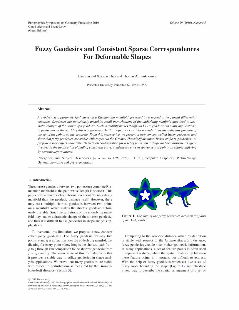
Figure 1: The sum of the fuzzy geodesics between all pairs

of marked points.

Comparing to the geodesic distance which by definitionis stable with respect to the Gromov-Hausdorff distance,fuzzy geodesics encode much richer geometric information.In many applications, a set of feature points is often usedto represent a shape, where the spatial relationship betweenthese feature points is important, but difficult to express.With the help of fuzzy geodesics which act like a set offuzzy ropes bounding the shape (Figure 1), we introducea new way to describe the spatial arrangement of a set of

c© 2010 The Author(s)Journal compilation c© 2010 The Eurographics Association and Blackwell Publishing Ltd.Published by Blackwell Publishing, 9600 Garsington Road, Oxford OX4 2DQ, UK and350 Main Street, Malden, MA 02148, USA.

J. Sun & X. Chen & T. A. Funkhouser / Fuzzy Geodesics and Consistent Sparse Correspondences For Deformable Shapes

points on a manifold using the intersection pattern of pair-wise fuzzy geodesics, which we call intersection config-

uration(Section 4). We find that differences in this inter-

section configuration are effective at distinguishing correctpoint correspondences from incorrect ones during experi-ments with a variety of meshes differing by extreme defor-mations (Section 5).

2. Background and related work

A geodesic on a Riemmannian manifold M is a curve γ :I →M such that the changing rate of the tangent vector of γ(given by the covariant derivative) vanishes at any point on γ.The geodesic is a classical concept in differential geometryand has been studied extensively [dC92]. The geodesic dis-tance between any two points p,q ∈M, denoted as dM(x,y),is the infimum of the lengths of all path joining p,q. Ifthe manifold M is complete, there must exist a minimiz-ing geodesic joining p,q that attains the geodesic distance,which we will call the geodesic between p,q for the remain-der of the paper.

In the discrete setting, computing the geodesics has beenstudied extensively [Pap85]. Mitchell et al. [MMP87] pre-sented an algorithm to compute the shortest geodesic be-tween any two points on a polygonal surface, and Surazhskyet al. proposed a fast implementation [SSK∗05]. Dijkstra’salgorithm can also be used to find approximate geodesics byworking with a graph formed by the mesh’s 1-skeleton.

The convergence of geodesics has also been stud-ied [HPW06, DL09], where a discrete representation (e.g.,polygonal surface or point set) is considered as an ap-proximation of some smooth manifold. The convergence ofgeodesics studies if a shortest path on the discrete represen-tation converge to a geodesic on the smooth manifold whenthe approximation error of the discrete representation to thesmooth manifold goes to zero. Hildebrandt et al [HPW06]and Dey and Li [DL09] show the subsequence convergenceof geodesics from polygonal surfaces and point clouds re-spectively.

However, the convergence of geodesics does not imply itis stable. In particular, geodesics are not stable at cut points.A cut point of a geodesic γ issued from the point p is thepoint where γ ceases to be minimizing. The cut locus of p

is all cut points on the geodesics issued from p. If there aremultiple geodesics between p,q, then p is on the cut locus

of q and vice verse. Therefore, if a geodesic passing throughtwo points that are close to each other’s cut locus, small per-turbations may lead to dramatic change of that geodesic.

3. Fuzzy Geodesics

In this section, we define fuzzy geodesics, and show theirstability with respect to perturbations.

Definition: To define fuzzy geodesics, let us consider the

image of the geodesic γ on the manifold M, also denotedas γ. The indicator function of γ, denoted as χγ, is definedas follows: χγ(x) = 1 if x ∈ γ and 0 otherwise. The indica-tor function χγ is an equivalent representation of γ. The ideaof fuzzy geodesic is basically to obtain a smoothed indica-tor function. However, naively smoothing the indicator func-tion will not make it stable due to the existence of multipleminimizing geodesics between two points. To overcome thisproblem, we introduce the fuzzy geodesic, which is definedas follows.

Definition 3.1 Given a parameter σ> 0, the fuzzy geodesicbetween any two points p and q on a Riemannian manifold

M is defined as a function Gσp,q : M → R:

Gσp,q(x) = exp

(

−|dM(x, p)+dM(x,q)−dM(p,q)|

σ

)

. (1)

Intuitively, the fuzzy geodesic Gσp,q(x) indicates for every

point x how long is the shortest path from p to q through x

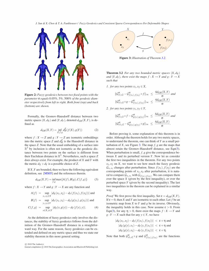
in comparison to the shortest geodesic from p to q directly.It attains the maximum value of one at points on the short-est geodesic(s) between p and q and less values (betweenzero and one) at other points (Figure 2). If there are multipleshortest geodesics, Gσ

p,q(x) reaches maximum on all of them.

The parameter σ controls the fuzziness. The bigger the σ

is, the fuzzier fuzzy geodesics are. In the extreme, when σ

goes to infinity, Gσp,q becomes a constant function 1. When

σ goes to 0, Gσp,q(x) becomes the indicator function of all

minimizing geodesics between p,q. In between, larger val-ues of σ produce fuzzy geodesics with larger values at pointsfurther from the shortest geodesics (Figure 2).

The time complexity of computing the fuzzy geodesicbetween two points is the same as that of computing thegeodesic distance from two sources to all other points. Inparticular, on a triangle mesh with n vertices, if we use Di-jkstra’s algorithm to approximate geodesic distance over the1-skeleton of the mesh, the complexity of computing fuzzygeodesic between a pair of points is O(n logn).

It should be noted that the fuzzy geodesics definition isvery general (it depends only on a distance metric), and thusfuzzy geodesics can be computed for a wide variety of inputtypes, including meshes, point clouds, graphs, etc., as longas a distance between points can be defined.

Stability: To analyze the stability of fuzzy geodesics, weconsider how the fuzzy geodesic function changes in re-lation to the Gromov-Hausdorff distance as a shape de-forms [Gro99]. The Gromov-Hausdorff distance is com-monly used to measure shape deformations [MS05,SMC07],and thus it provides a good measure for how similar twoshapes are. Our goal is to show that two shapes with a smallGromov-Hausdorff distance provably have a small differ-ence in their fuzzy geodesics.

c© 2010 The Author(s)Journal compilation c© 2010 The Eurographics Association and Blackwell Publishing Ltd.


Figure 2: Fuzzy geodesics between two fixed points with the

parameter σ equals 0.05%, 5%, 500% of the geodesic diam-

eter respectively from left to right. Both front (top) and back

(bottom) are shown.

Formally, the Gromov-Hausdorff distance between twometric spaces (X ,dX ) and (Y,dY ), denoted dGH(X ,Y ), is de-fined as

dGH(X ,Y ) = infZ, f ,g

dZH( f (X),g(Y )) (2)

where f : X → Z and g : Y → Z are isometric embeddingsinto the metric space Z and dZH is the Hausdorff distance inthe space Z. Note that the usual embedding of a surface intoR

3 by inclusion is often not isometric as the geodesic dis-tance between two points on the surface is different fromtheir Euclidean distance in R

3. Nevertheless, such a space Z

does always exist. For example, the product of X and Y withthe metric dX +dY is a possible choice of Z.

If X ,Y are bounded, then we have the following equivalentdefinition, see [MS05] and the references therein.

dGH(X ,Y ) = inff ,g

max{A( f ),B(g),C( f ,g)} (3)

where f : X → Y and g : Y → X are any function and

A( f ) = supx1,x2∈X

|dX (x1,x2)−dY ( f (x1), f (x2))| and

B( f ) = supy1,y2∈Y

|dY (y1,y2)−dX (g(y1),g(y2))| and

C( f ,g) = supx∈X ,y∈Y

|dX (x,g(y))−dY ( f (x),y)|. (4)

As the definition of fuzzy geodesics only involves the dis-tances, the stability of fuzzy geodesics follows from the def-inition of the Gromov-Hausdorff distance in a straightfor-ward way. For the same reason, fuzzy geodesics can be ex-tended and defined on any metric space and thus we state ourstability theorem in this more general setting.

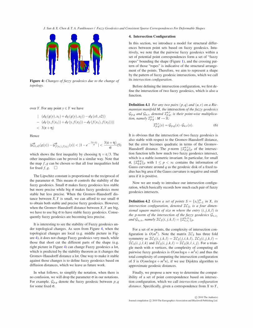
X Y

f

g

x2

x1

f(x2)

f(x1)

Figure 3: Illustration of Theorem 3.2.

Theorem 3.2 For any two bounded metric spaces (X ,dX )and (Y,dY ), there exist the maps f : X → Y and g : Y → X

such that

1. for any two points x1,x2 ∈ X,

‖Gσx1,x2 −Gσ

f (x1), f (x2)◦ f‖∞ ≤

4dGH(X ,Y )

σand

‖Gσx1,x2 ◦g−Gσ

f (x1), f (x2)‖∞ ≤

4dGH(X ,Y )

σ.

2. for any two points y1,y2 ∈ Y ,

‖Gσy1,y2 ◦ f −Gσ

g(y1),g(y2)‖∞ ≤

4dGH(X ,Y )

σand

‖Gσy1,y2 −Gσ

g(y1),g(y2)◦g‖∞ ≤

4dGH(X ,Y )

σ.

Before proving it, some explanation of this theorem is inorder. Although the theorem holds for any two metric spaces,to understand the theorem, one can think of Y as a small per-turbation of X , see Figure 3. The map f ,g are the maps thatalmost retain the Gromov-Hausdorff distance, see Eqn(3).When perturbation is small, f ,g give the correspondence be-tween X and its perturbed version Y . Now let us considerthe first two inequalities in the theorem. For any two pointsx1,x2 on X , we want to see how much the fuzzy geodesicGx1,x2 changes after perturbation. Since f (x1), f (x2) are thecorresponding points of x1,x2 after perturbation, it is natu-ral to compare Gx1,x2 with G f (x1), f (x2). We can compare themover the space X (given by the first inequality), or over theperturbed space Y (given by the second inequality). The lasttwo inequalities in the theorem can be explained in a similarway.

Proof We first prove the first inequality. Set ε = dGH(X ,Y ).If ε= 0, then X andY are isometric to each other. Let f be anisometric map from X to Y and g be its inverse. Obviously,the inequality holds in this case. Now assume ε > 0. FromEqn(3), for any η > 0, there exist the maps f : X → Y andg : Y → X such that for any y ∈ Y , we have

|dX (x1,x2)−dY ( f (x1), f (x2))| < ε+η and

|dX (g(y),x1)−dY (y, f (x1))| < ε+η and

|dX (g(y),x2)−dY (y, f (x2))| < ε+η.

Note that both Gσx1,x2 ◦ g and Gσ

f (x1), f (x2)are the functions



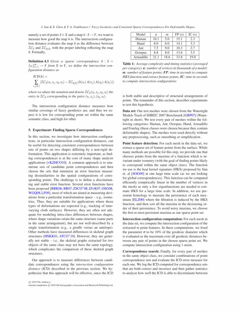
Figure 4: Changes of fuzzy geodesics due to the change of

topology.

over Y . For any point y ∈ Y we have

| (dX (g(y),x1)+dX (g(y),x2))−dX (x1,x2))

− (dY (y, f (x1))+dY (y, f (x2))−dY ( f (x1), f (x2)))|

< 3(ε+η)

Hence

|Gσx1,x2(g(y))−Gσ

f (x1), f (x2)(y)| < |1− e

−3(ε+η)

σ | <3(ε+η)

σ(5)

which shows the first inequality by choosing η = ε/3. Theother inequalities can be proved in a similar way. Note thatthe map f ,g can be chosen so that all four inequalities holdfor fixed f ,g.

The Lipschitz constant is proportional to the reciprocal ofthe parameter σ. This means σ controls the stability of thefuzzy geodesics. Small σ makes fuzzy geodesics less stablebut more precise while big σ makes fuzzy geodesics morestable but less precise. When the Gromov-Hausdorff dis-tance between X ,Y is small, we can afford to use small σto obtain both stable and precise fuzzy geodesics. However,when the Gromov-Hausdorff distance between X ,Y are big,we have to use big σ to have stable fuzzy geodesics. Conse-quently fuzzy geodesics are becoming less precise.

It is interesting to see the stability of Fuzzy geodesics un-der topological changes. As seen from Figure 4, when thetopological changes are local (e.g. middle picture in Fig-ure 4), it does not change Fuzzy geodesics very much, whilethose that short cut the different parts of the shape (e.g.right picture in Figure 4) can change Fuzzy geodesics a lot,which is predicted by the stability theorem as it changes theGromov-Hausdorff distance a lot. One way to make it stableagainst those changes is to define fuzzy geodesics based ondiffusion distances, which we leave as future work.

In what follows, to simplify the notation, when there isno confusion, we will drop the parameter σ in our notations.For example. Gp,q denote the fuzzy geodesic between p,qfor some fixed σ.

4. Intersection Configuration

In this section, we introduce a model for structural differ-ences between point sets based on fuzzy geodesics. Intu-itively, we note that the pairwise fuzzy geodesics within aset of potential point correspondences form a set of “fuzzyropes” bounding the shape (Figure 1), and the crossing pat-tern of those “ropes” is indicative of the structural arrange-ment of the points. Therefore, we aim to represent a shapeby the pattern of fuzzy geodesic intersections, which we callits intersection configuration.

Before defining the intersection configuration, we first de-fine the intersection of two fuzzy geodesics, which is also afunction.

Definition 4.1 For any two pairs (p,q) and (u,v) on a Rie-

mannian manifold M, the intersection of the fuzzy geodesics

Gp,q and Gu,v, denoted Iu,vp,q, is their point-wise multiplica-

tion, namely Iu,vp,q : M → R:

Iu,vp,q(x) = Gp,q(x) · Gu,v(x). (6)

It is obvious that the intersection of two fuzzy geodesics isalso stable with respect to the Gromov-Hausdorff distance,but the error becomes quadratic in terms of the Gromov-Hausdorff distance. The p-norm ‖Iu,v

p,q‖p of the intersec-tion function tells how much two fuzzy geodesics intersect,which is a stable isometric invariant. In particular, for smallσ, ‖Iq,q

q,q‖p with 1 ≤ p < ∞ contains the information ofGauss curvature around q as the geodesic disk of a fixed ra-dius has big area if the Gauss curvature is negative and smallarea if it is positive.

Now we are ready to introduce our intersection configu-ration, which basically records how much each pair of fuzzygeodesics intersects.

Definition 4.2 Given a set of points S = {si}mi=1 in X, its

intersection configuration, denoted ICS, is a four dimen-

sional square matrix of size m where the entry (i, j,k, l) is

the p-norm of the intersection of the fuzzy geodesics Gsi,s j

and Gsk,sl , namely ICS(i, j,k, l) = ‖Isk,slsi,s j ‖p.

For a set of m points, the complexity of intersection con-figuration is O(m4). Note the matrix ICS has three foldsymmetry as ICS(i, j,k, l) = ICS( j, i,k, l), ICS(i, j,k, l) =ICS(i, j, l,k) and ICS(i, j,k, l) = ICS(k, l, i, j). For a trian-gle mesh with n vertices, the complexity of computing allpairwise fuzzy geodesics is O(mn logn+m2n) and thus thetotal complexity of computing the intersection configurationof S is O(mn logn+m4n), if we use Dijsktra algorithm toapproximate geodesic distances.

Finally, we propose a new way to determine the compat-ibility of a set of point correspondence based on intersec-tion configuration, which we call intersection configuration

distance. Specifically, given a correspondence from X to Y ,



namely a set of points S∈ X and a map h : S→Y , we want tomeasure how good the map h is. The intersection configura-tion distance evaluates the map h as the difference betweenICS and ICh(S) with the proper labeling reflecting the maph. Formally,

Definition 4.3 Given a sparse correspondence h : S ={si}

mi=1 → Y from X to Y , we define the intersection con-

figuration distance as

ICD(h) =

∑i, j,k,l

|ICS(si,s j,sk,sl)−ICh(S)(h(si),h(s j),h(sk),h(sl))|

where we abuse the notation and denote ICS(si,s j,sk,sl) theentry in ICS corresponding to the pairs (si,s j),(sk,sl).

The intersection configuration distance measures howsimilar crossings of fuzzy geodesics are, and thus we ex-pect it is low for corresponding point set within the samesemantic class, and high for other

5. Experiment: Finding Sparse Correspondences

In this section, we investigate how intersection configura-tions, in particular intersection configuration distances, canbe useful for detecting consistent correspondences betweensets of points on two shapes differing by a non-rigid de-formation. This application is extremely important, as find-ing correspondences is at the core of many shape analysisapplications [vKZHCO10]. A common approach is to enu-merate sets of candidate point correspondences and thenchoose the sets that minimize an error function measur-ing dissimilarities in the spatial configurations of corre-sponding points. The challenge is to define a discriminat-ing and stable error function. Several error functions havebeen proposed [BBK06, BR07, ZSCO∗08, JZvK07, OSG08,WGQ08,LF09], most of which are aimed at measuring devi-ations from a particular transformation space – e.g., isome-tries. Thus, they are suitable for applications where thosetypes of deformations are expected (e.g., tracking of time-varying cloth surfaces). However, they are often not ade-quate for modeling intra-class differences between shapes,where shape variations retain the same structure (same partsin the same arrangement), but are not well-described by asingle transformation (e.g., a giraffe versus an antelope).Other methods have measured differences in skeletal graphstructures [HSKK01, ATCO∗10]. However, they are gener-ally not stable – i.e., the skeletal graphs extracted for twoobjects of the same class may not have the same topology,which complicates the comparison of these skeletal graphstructures.

Our approach is to measure differences between candi-date correspondences using the intersection configuration

distance (ICD) described in the previous section. We hy-pothesize that this approach will be effective, since the ICD

Model n m FP (s) IC (s)Human 10.1 5.0 15.1 2.3Hand 8.0 6.0 14.1 3.3Ant 7.5 9.0 10.3 2.7

Octopus 8.8 8.0 13.6 3.5Armadillo 21.1 18.6 33.8 19.0

Table 1: Average complexity and timing statistics (averaged

per category). n: number of vertices in thousands of a model;

m: number of feature points; FP: time in seconds to compute

HKS function and extract feature points; IC: time in seconds

to compute intersection configuration;

is both stable and descriptive of structural arrangements ofpoints. The remainder of this section, describes experimentsto test this hypothesis.

Data set: Our test meshes were chosen from the WatertightModels Track of SHREC 2007 Benchmark [GBP07] (Water-tight in short). We test every pair of meshes within the fol-lowing categories: Human, Ant, Octopus, Hand, Armadilloand Fourleg (these classes were chosen because they containdeformable shapes). The meshes were used directly withoutany preprocessing, such as smoothing or simplification .

Point feature detection: For each mesh in the data set, weextract a sparse set of feature points from the surface. Whilemany methods are possible for this step, we provide one thatchooses points from the maxima of a function which is in-variant under isometry (with the goal of finding points likelyto correspond within the same object class). The functionwe use is the heat kernel signature (HKS) proposed by Sunet. al [SOG09] at one large time scale (as we are lookingfor global correspondences). This function can be computedefficiently (empirically linear in the number of vertices inthe mesh) as only a few eigenfunctions are needed to esti-mate HKS for a large time scale. In addition, we use per-sistent homology to measure the persistence of each max-imum [ELZ00] where the filtration is induced by the HKSfunction, and then sort all the maxima in the decreasing or-der of their persistence. To avoid noisy maxima, we choosethe first m most persistent maxima as our sparse point set.

Intersection configuration computation: For each mesh inthe data set, we compute the intersection configuration of theextracted m point features. In these computations, we fixedthe parameter σ to be 10% of the geodesic diameter whichis evaluated as the maximum over all geodesic distances be-tween any pair of points in the chosen sparse point set. Wecompute intersection configuration using 1-norm.

Correspondence search: Finally, for every pair of meshesin the same object class, we consider combinations of pointcorrespondence sets and evaluate the ICD error measure foreach one. We log the ICD computed for correspondence setsthat are both correct and incorrect and then gather statisticsto analyze how well the ICD is able to discriminate between



Oct

opus

0

0.2

0.4

0.6

0.8

1

Pro

po

rtio

n o

f m

esh

pa

irs

20

21

22

23

24

25

26

27

28

29

210

211

212

Geodesic DistanceICD

0 5 10 150

0.1

0.2

0.3

0.4

0.5

0.6

0.7

Pro

port

ion o

f m

esh p

airs

0

0.2

0.4

0.6

0.8

24

25

26

27

28

29

210

211

212

213

214

215

Pro

port

ion o

f m

esh p

airs

Ant

0

0.2

0.4

0.6

0.8

1

20

21

22

23

24

25

26

27

28

29

Pro

port

ion o

f m

esh p

airs

0 1 20

0.2

0.4

0.6

0.8

1

Pro

port

ion o

f m

esh p

airs

0

0.2

0.4

0.6

0.8

1

21

22

23

24

25

26

27

28

29

Pro

port

ion o

f m

esh p

airs

Hum

an

0

0.2

0.4

0.6

0.8

1

20

21

22

23

24

Pro

port

ion o

f m

esh p

airs

0 1 20

0.2

0.4

0.6

0.8

Pro

port

ion o

f m

esh p

airs

0

0.2

0.4

0.6

0.8

1

21

22

23

24

Pro

port

ion o

f m

esh p

airs

Han

d

0

0.1

0.2

0.3

0.4

0.5

20

21

22

23

24

25

26

27

28

29

Pro

port

ion o

f m

esh p

airs

0 10

0.2

0.4

0.6

0.8

Pro

port

ion o

f m

esh p

airs

0

0.1

0.2

0.3

0.4

0.5

20

21

22

23

24

25

26

27

28

29

Pro

port

ion o

f m

esh p

airs

(1) (2) (3)

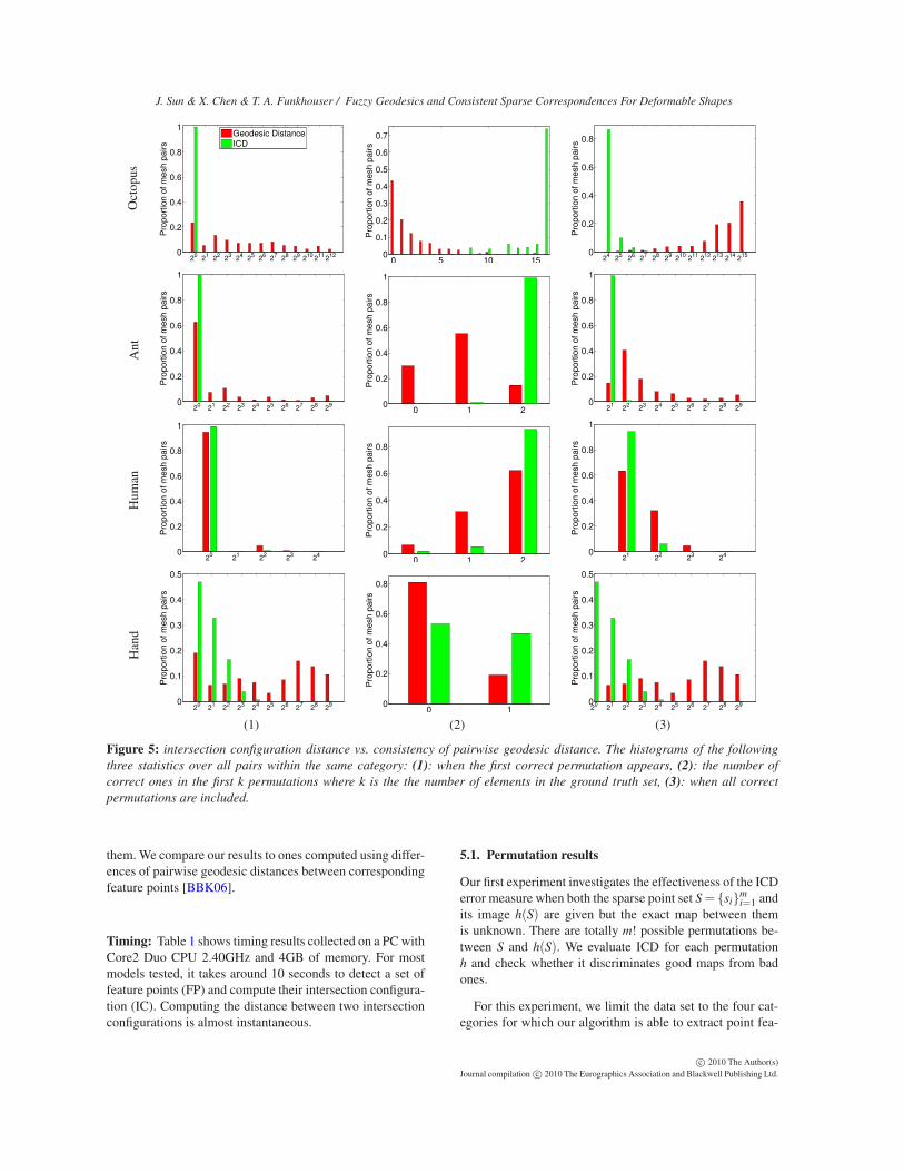
Figure 5: intersection configuration distance vs. consistency of pairwise geodesic distance. The histograms of the following

three statistics over all pairs within the same category: (1): when the first correct permutation appears, (2): the number of

correct ones in the first k permutations where k is the the number of elements in the ground truth set, (3): when all correct

permutations are included.

them. We compare our results to ones computed using differ-ences of pairwise geodesic distances between correspondingfeature points [BBK06].

Timing: Table 1 shows timing results collected on a PC withCore2 Duo CPU 2.40GHz and 4GB of memory. For mostmodels tested, it takes around 10 seconds to detect a set offeature points (FP) and compute their intersection configura-tion (IC). Computing the distance between two intersectionconfigurations is almost instantaneous.

5.1. Permutation results

Our first experiment investigates the effectiveness of the ICDerror measure when both the sparse point set S= {si}

mi=1 and

its image h(S) are given but the exact map between themis unknown. There are totally m! possible permutations be-tween S and h(S). We evaluate ICD for each permutationh and check whether it discriminates good maps from badones.

For this experiment, we limit the data set to the four cat-egories for which our algorithm is able to extract point fea-



1R 2R 3R

4R

5R6R7R

0R = Id

Rot

1R 2R 3R

4R

5R6R7R

0R = Id

Ref

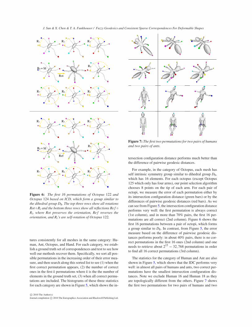
Figure 6: The first 16 permutations of Octopus 122 and

Octopus 124 based on ICD, which form a group similar to

the dihedral group D8. The top three rows show all rotations

Rot ◦Ri and the bottom three rows show all reflections Re f ◦Ri, where Rot preserves the orientation, Re f reverses the

orientation, and Ri’s are self-rotation of Octopus 122.

tures consistently for all meshes in the same category: Hu-man, Ant, Octopus, and Hand. For each category, we estab-lish a ground truth set of correspondences and test to see howwell our methods recover them. Specifically, we sort all pos-sible permutations in the increasing order of their error mea-sure, and then search along this sorted list to see (1) when thefirst correct permutation appears, (2) the number of correctones in the first k permutations where k is the the number ofelements in the ground truth set, (3) when all correct permu-tations are included. The histograms of these three statisticsfor each category are shown in Figure 5, which shows the in-

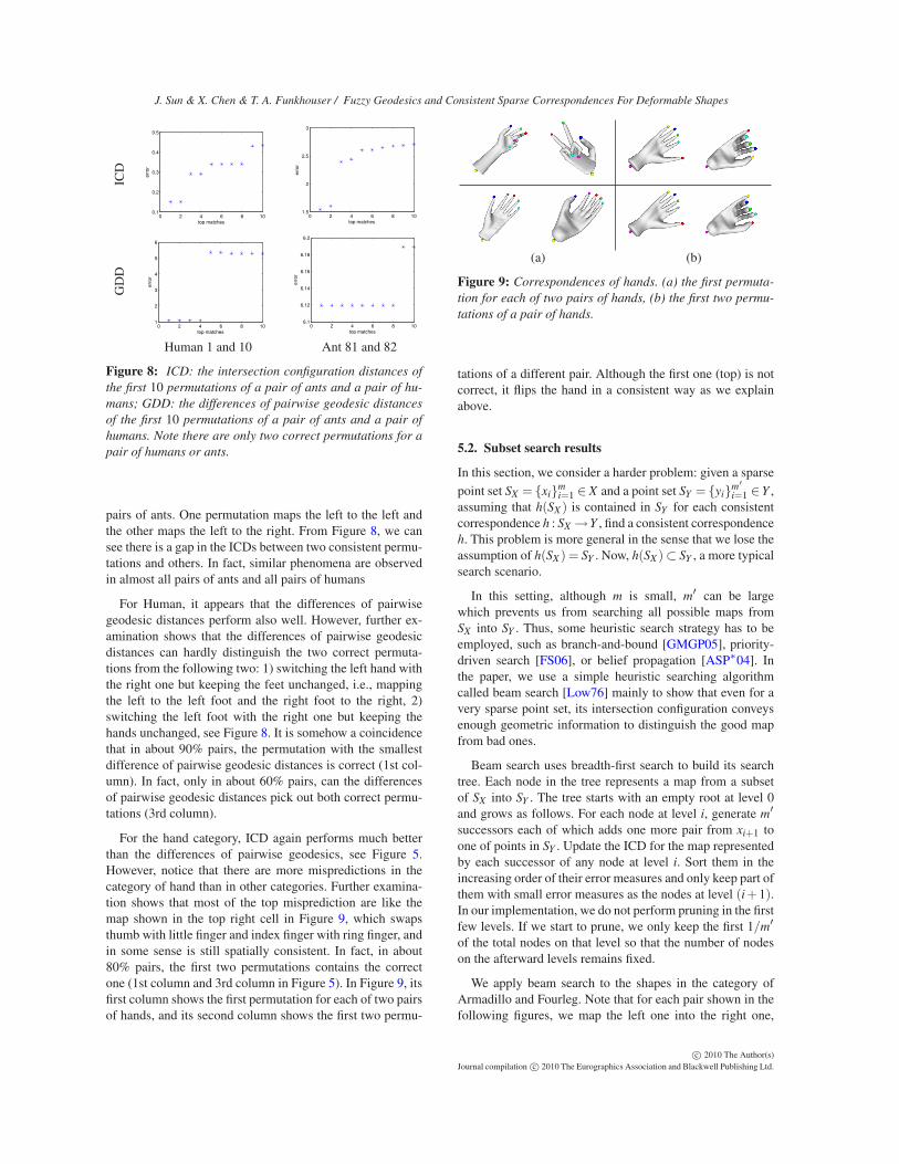
Figure 7: The first two permutations for two pairs of humans

and two pairs of ants.

tersection configuration distance performs much better thanthe difference of pairwise geodesic distances.

For example, in the category of Octopus, each mesh hasself intrinsic symmetry group similar to dihedral group D8,which has 16 elements. For each octopus (except Octopus125 which only has four arms), our point selection algorithmchooses 8 points on the tip of each arm. For each pair ofoctopi, we measure the error of each permutation either byits intersection configuration distance (green bars) or by thedifferences of pairwise geodesic distances (red bars). As wecan see from Figure 5, the intersection configuration distanceperforms very well: the first permutation is always correct(1st column), and in more than 70% pairs, the first 16 per-mutations are all correct (2nd column). Figure 6 shows thefirst 16 permutations between a pair of octopi, which formsa group similar to D8. In contrast, from Figure 5, the errormeasure based on the difference of pairwise geodesic dis-tances performs poorly: in about 40% pairs, there is no cor-rect permutations in the first 16 ones (2nd column) and oneneeds to retrieve about 215 = 32,768 permutations in orderto find all 16 correct permutations (3rd column).

The statistics for the category of Human and Ant are alsoshown in Figure 5, which shows that the IDC performs verywell: in almost all pairs of humans and ants, two correct per-mutations have the smallest intersection configuration dis-tances. Note we exclude Human 16 and Human 18 as theyare topologically different from the others. Figure 7 showsthe first two permutations for two pairs of humans and two



ICD

0 2 4 6 8 100.1

0.2

0.3

0.4

0.5

top matches

err

or

0 2 4 6 8 101.5

2

2.5

3

top matches

err

or

GD

D

0 2 4 6 8 101

2

3

4

5

6

top matches

err

or

0 2 4 6 8 106.1

6.12

6.14

6.16

6.18

6.2

top matches

err

or

Human 1 and 10 Ant 81 and 82

Figure 8: ICD: the intersection configuration distances of

the first 10 permutations of a pair of ants and a pair of hu-

mans; GDD: the differences of pairwise geodesic distances

of the first 10 permutations of a pair of ants and a pair of

humans. Note there are only two correct permutations for a

pair of humans or ants.

pairs of ants. One permutation maps the left to the left andthe other maps the left to the right. From Figure 8, we cansee there is a gap in the ICDs between two consistent permu-tations and others. In fact, similar phenomena are observedin almost all pairs of ants and all pairs of humans

For Human, it appears that the differences of pairwisegeodesic distances perform also well. However, further ex-amination shows that the differences of pairwise geodesicdistances can hardly distinguish the two correct permuta-tions from the following two: 1) switching the left hand withthe right one but keeping the feet unchanged, i.e., mappingthe left to the left foot and the right foot to the right, 2)switching the left foot with the right one but keeping thehands unchanged, see Figure 8. It is somehow a coincidencethat in about 90% pairs, the permutation with the smallestdifference of pairwise geodesic distances is correct (1st col-umn). In fact, only in about 60% pairs, can the differencesof pairwise geodesic distances pick out both correct permu-tations (3rd column).

For the hand category, ICD again performs much betterthan the differences of pairwise geodesics, see Figure 5.However, notice that there are more mispredictions in thecategory of hand than in other categories. Further examina-tion shows that most of the top misprediction are like themap shown in the top right cell in Figure 9, which swapsthumb with little finger and index finger with ring finger, andin some sense is still spatially consistent. In fact, in about80% pairs, the first two permutations contains the correctone (1st column and 3rd column in Figure 5). In Figure 9, itsfirst column shows the first permutation for each of two pairsof hands, and its second column shows the first two permu-

(a) (b)

Figure 9: Correspondences of hands. (a) the first permuta-

tion for each of two pairs of hands, (b) the first two permu-

tations of a pair of hands.

tations of a different pair. Although the first one (top) is notcorrect, it flips the hand in a consistent way as we explainabove.

5.2. Subset search results

In this section, we consider a harder problem: given a sparse

point set SX = {xi}mi=1 ∈ X and a point set SY = {yi}

m′

i=1 ∈Y ,assuming that h(SX ) is contained in SY for each consistentcorrespondence h : SX →Y , find a consistent correspondenceh. This problem is more general in the sense that we lose theassumption of h(SX ) = SY . Now, h(SX )⊂ SY , a more typicalsearch scenario.

In this setting, although m is small, m′ can be largewhich prevents us from searching all possible maps fromSX into SY . Thus, some heuristic search strategy has to beemployed, such as branch-and-bound [GMGP05], priority-driven search [FS06], or belief propagation [ASP∗04]. Inthe paper, we use a simple heuristic searching algorithmcalled beam search [Low76] mainly to show that even for avery sparse point set, its intersection configuration conveysenough geometric information to distinguish the good mapfrom bad ones.

Beam search uses breadth-first search to build its searchtree. Each node in the tree represents a map from a subsetof SX into SY . The tree starts with an empty root at level 0and grows as follows. For each node at level i, generate m′

successors each of which adds one more pair from xi+1 toone of points in SY . Update the ICD for the map representedby each successor of any node at level i. Sort them in theincreasing order of their error measures and only keep part ofthem with small error measures as the nodes at level (i+1).In our implementation, we do not perform pruning in the firstfew levels. If we start to prune, we only keep the first 1/m′

of the total nodes on that level so that the number of nodeson the afterward levels remains fixed.

We apply beam search to the shapes in the category ofArmadillo and Fourleg. Note that for each pair shown in thefollowing figures, we map the left one into the right one,



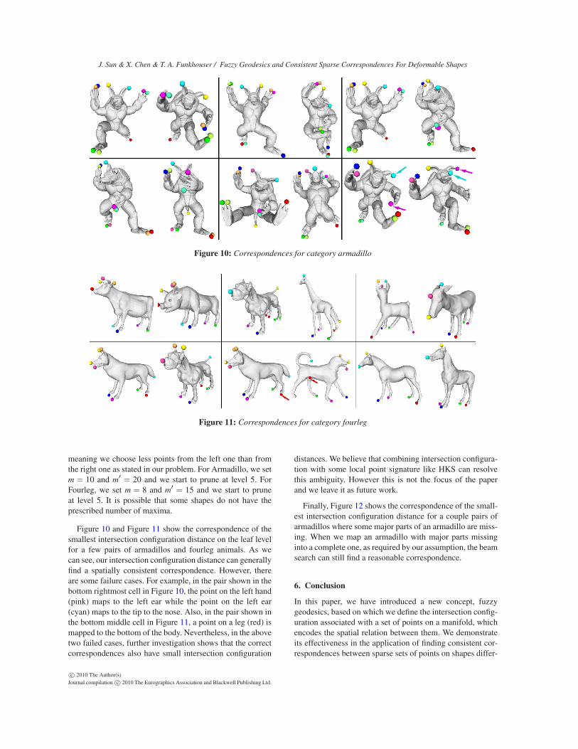
Figure 10: Correspondences for category armadillo

Figure 11: Correspondences for category fourleg

meaning we choose less points from the left one than fromthe right one as stated in our problem. For Armadillo, we setm = 10 and m′ = 20 and we start to prune at level 5. ForFourleg, we set m = 8 and m′ = 15 and we start to pruneat level 5. It is possible that some shapes do not have theprescribed number of maxima.

Figure 10 and Figure 11 show the correspondence of thesmallest intersection configuration distance on the leaf levelfor a few pairs of armadillos and fourleg animals. As wecan see, our intersection configuration distance can generallyfind a spatially consistent correspondence. However, thereare some failure cases. For example, in the pair shown in thebottom rightmost cell in Figure 10, the point on the left hand(pink) maps to the left ear while the point on the left ear(cyan) maps to the tip to the nose. Also, in the pair shown inthe bottom middle cell in Figure 11, a point on a leg (red) ismapped to the bottom of the body. Nevertheless, in the abovetwo failed cases, further investigation shows that the correctcorrespondences also have small intersection configuration

distances. We believe that combining intersection configura-tion with some local point signature like HKS can resolvethis ambiguity. However this is not the focus of the paperand we leave it as future work.

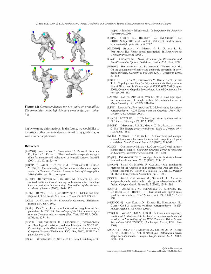
Finally, Figure 12 shows the correspondence of the small-est intersection configuration distance for a couple pairs ofarmadillos where some major parts of an armadillo are miss-ing. When we map an armadillo with major parts missinginto a complete one, as required by our assumption, the beamsearch can still find a reasonable correspondence.

6. Conclusion

In this paper, we have introduced a new concept, fuzzygeodesics, based on which we define the intersection config-uration associated with a set of points on a manifold, whichencodes the spatial relation between them. We demonstrateits effectiveness in the application of finding consistent cor-respondences between sparse sets of points on shapes differ-



Figure 12: Correspondences for two pairs of armadillos.

The armadillos on the left side have some major parts miss-

ing.

ing by extreme deformations. In the future, we would like toinvestigate other theoretical properties of fuzzy geodesics, aswell as other applications.

References

[ASP∗04] ANGUELOV D., SRINIVASAN P., PANG H., KOLLER

D., THRUN S., DAVIS J.: The correlated correspondence algo-rithm for unsupervised registration of nonrigid surfaces. In NIPS

(2004), vol. 17, pp. 33–40.

[ATCO∗10] AU O. K.-C., TAI C.-L., COHEN-OR D., ZHENG

Y., FU H.: Electors voting for fast automatic shape correspon-dence. In Computer Graphics Forum (In Proc. of Eurographics

2010) (2010), vol. 29, p. to appear.

[BBK06] BRONSTEIN A., BRONSTEIN M., KIMMEL R.: Gen-eralized multidimensional scaling: A framework for isometry-invariant partial surface matching. Proceedings of the National

Academy of Science (2006), 1168–1172.

[BR07] BROWN B. J., RUSINKIEWICZ S.: Global non-rigidalignment of 3-d scans. ACM Trans. Graph. 26, 3 (2007), 21.

[dC92] DO CARMO M. P.: Riemannian Geometry. Birkhäuser,Boston, MA, USA, 1992.

[DL09] DEY T. K., LI K.: Cut locus and topology from surfacepoint data. In SCG ’09: Proceedings of the 25th annual sympo-

sium on Computational geometry (New York, NY, USA, 2009),ACM, pp. 125–134.

[ELZ00] EDELSBRUNNER H., LETSCHER D., ZOMORODIAN

A.: Topological persistence and simplification. In FOCS ’00:

Proceedings of the 41st Annual Symposium on Foundations of

Computer Science (Washington, DC, USA, 2000), IEEE Com-puter Society, p. 454.

[FS06] FUNKHOUSER T., SHILANE P.: Partial matching of 3d

shapes with priority-driven search. In Symposium on Geometry

Processing (2006).

[GBP07] GIORGI D., BIASOTTI S., PARABOSCHI L.:SHREC:SHape REtrieval Contest: Watertight models track,http://watertight.ge.imati.cnr.it/, 2007.

[GMGP05] GELFAND N., MITRA N. J., GUIBAS L. J.,POTTMANN H.: Robust global registration. In Symposium on

Geometry Processing (2005).

[Gro99] GROMOV M.: Metric Structures for Riemannian and

Non-Riemannian Spaces. Birkhäuser, Boston, MA, USA, 1999.

[HPW06] HILDEBRANDT K., POLTHIER K., WARDETZKY M.:On the convergence of metric and geometric properties of poly-hedral surfaces. Geometriae Dedicata 123, 1 (December 2006),89–112.

[HSKK01] HILAGA M., SHINAGAWA Y., KOHMURA T., KUNII

T. L.: Topology matching for fully automatic similarity estima-tion of 3D shapes. In Proceedings of SIGGRAPH 2001 (August2001), Computer Graphics Proceedings, Annual Conference Se-ries, pp. 203–212.

[JZvK07] JAIN V., ZHANG H., VAN KAICK O.: Non-rigid spec-tral correspondence of triangle meshes. International Journal onShape Modeling 13, 1 (2007), 101–124.

[LF09] LIPMAN Y., FUNKHOUSER T.: Mobius voting for surfacecorrespondence. ACM Transactions on Graphics (Proc. SIG-

GRAPH) 28, 3 (August 2009).

[Low76] LOWERRE B. T.: The harpy speech recognition system.

PhD thesis, Pittsburgh, PA, USA, 1976.

[MMP87] MITCHELL J. S. B., MOUNT D. M., PAPADIMITRIOU

C. H.: The discrete geodesic problem. SIAM J. Comput. 16, 4(1987), 647–668.

[MS05] MÉMOLI F., SAPIRO G.: A theoretical and compu-tational framework for isometry invariant recognition of pointcloud data. Found. Comput. Math. 5, 3 (2005), 313–347.

[OSG08] OVSJANIKOV M., SUN J., GUIBAS L.: Global intrinsicsymmetries of shapes. Computer Graphics Forum (Symposium

on Geometry Processing) 27, 5 (2008), 1341–1348.

[Pap85] PAPADIMITRIOU C.: An algorithm for shortest-path mo-tion in three dimensions. IPL 20 (1985), 259–163.

[SMC07] SINGH G., MEMOLI F., CARLSSON G.: TopologicalMethods for the Analysis of High Dimensional Data Sets and 3DObject Recognition. Botsch M., Pajarola R., Chen B., ZwickerM., (Eds.), Eurographics Association, pp. 91–100.

[SOG09] SUN J., OVSJANIKOV M., GUIBAS L. J.: A conciseand provably informative multi-scale signature based on heat dif-fusion. Comput. Graph. Forum 28, 5 (2009), 1383–1392.

[SSK∗05] SURAZHSKY V., SURAZHSKY T., KIRSANOV D.,GORTLER S. J., HOPPE H.: Fast exact and approximategeodesics on meshes. ACM Trans. Graph. 24, 3 (2005), 553–560.

[vKZHCO10] VAN KAICK O., ZHANG H., HAMARNEH G.,COHEN-OR D.: A survey on shape correspondence. In EU-

ROGRAPHICS STAR Report (2010).

[WGQ08] WANG S., GU X., QIN H.: Automatic non-rigid reg-istration of 3d dynamic data for facial expression synthesis andtransfer. In Proceedings of the IEEE Computer Vision Pattern

Recognition 2008 (CVPR08) (Anchorage, Alaska, USA, June2008).

[ZSCO∗08] ZHANG H., SHEFFER A., COHEN-OR D., ZHOU

Q., VAN KAICK O., TAGLIASACCHI A.: Deformation-drivenshape correspondence. Comput. Graph. Forum 27, 5 (2008),1431–1439.


Documents

Fuzzy Geodesics and Consistent Sparse …funk/fuzzy_geodesics.pdfFuzzy Geodesics and Consistent Sparse Correspondences ... A geodesic is a parameterized curve ... Fuzzy Geodesics and