Embed Size (px)
Citation preview

FOCUS
Fuzzy knowledge representation study for incremental learningin data streams and classification problems
Albert Orriols-Puig • Jorge Casillas
Published online: 1 December 2010
� Springer-Verlag 2010
Abstract The extraction of models from data streams has
become a hot topic in data mining due to the proliferation
of problems in which data are made available online. This
has led to the design of several systems that create data
models online. A novel approach to online learning of data
streams can be found in Fuzzy-UCS, a young Michigan-
style fuzzy-classifier system that has recently demonstrated
to be highly competitive in extracting classification models
from complex domains. Despite the promising results
reported for Fuzzy-UCS, there still remain some hot issues
that need to be analyzed in detail. This paper carefully
studies two key aspects in Fuzzy-UCS: the ability of the
system to learn models from data streams where concepts
change over time and the behavior of different fuzzy
representations. Four fuzzy representations that move
through the dimensions of flexibility and interpretability
are included in the system. The behavior of the different
representations on a problem with concept changes is
studied and compared to other machine learning techniques
prepared to deal with these types of problems. Thereafter,
the comparison is extended to a large collection of real-
world problems, and a close examination of which problem
characteristics benefit or affect the different representations
is conducted. The overall results show that Fuzzy-UCS can
effectively deal with problems with concept changes and
lead to different interesting conclusions on the particular
behavior of each representation.
Keywords Fuzzy rule-based representation �Genetic algorithms � Learning classifier systems �Genetic fuzzy systems � Data streams � Concept drift
1 Introduction
In the last few years, the need to extract novel information
from data streams has led to the design of different
incremental learning architectures that can create data
models online as new examples are coming to the system
(Aggarwal 2007; del Campo-Avila et al. 2008; Gama and
Gaber 2007). This type of learning has received especial
attention not only because it enables practitioners to extract
key information from problems in which data are contin-
uously generated and where concepts may change over
time, e.g., stock market and sensor data among others, but
also because it enables them to deal with huge data sets
by making them available as data streams. Two common
approaches have been employed to deal with these types of
problems. On the one hand, several works have proposed
the use of time windows to store part of the—or the
entire—data stream, and then, the application of any batch
learning system to learn from this time window (Maloof
and Michalski 2004; Widmer and Kubat 1996; Gama et al.
2004). The key aspect in these types of systems is to define
the proper size of the time window, which has strong
implications on the runtime and the performance of the
system. That is, larger windows result in longer runtimes to
process all data. Also, enlarging or shrinking the window
controls the capacity of the system to forget past instances;
A. Orriols-Puig (&)
Grup de Recerca en Sistemes Intel�ligents, La Salle-Universitat
Ramon Llull, 08022 Barcelona, Spain
e-mail: [email protected]
J. Casillas
Department of Computer Science and Artificial Intelligence,
Research Center on Communication and Information
Technology (CITIC-UGR), University of Granada,
18071 Granada, Spain
e-mail: [email protected]
123
Soft Comput (2011) 15:2389–2414
DOI 10.1007/s00500-010-0668-x

this may cause important instances and noisy instances to
be included in or excluded from the learning process, and
thus, choosing a correct size of the window for each par-
ticular problem is the key for success in these approaches.
On the other hand, there have been some proposals of
systems that directly learn from the data stream without
using any instance memory (Angelov et al. 2008; Domingos
and Hulten 2000; Gama et al. 2003; Abbass et al. 2004;
Nunez et al. 2007).
A novel algorithm that falls under the last category is
Fuzzy-UCS (Orriols-Puig et al. 2008, 2009), a Michigan-
style learning fuzzy-classifier system (LFCS) that uses
genetic algorithms (GAs) (Holland 1975; Goldberg 1989)
to evolve independent-fuzzy-rule sets online from data
streams. The robustness and competitiveness of the system
was experimentally demonstrated over different real-
world problems where concepts did not vary over time
(Orriols-Puig et al. 2009). In addition, the advantages of
the online learning architecture of Fuzzy-UCS were
highlighted by evolving highly accurate models from large
data sets that were processed as data streams. Despite
these promising results, two key challenges that needed to
be addressed in further work were identified. First,
although the system’s architecture was originally designed
to learn from data streams, experiments were performed
on problems that did not present concept changes.
Therefore, further study on how Fuzzy-UCS adapts to
concept changes was pointed out as an interesting future
work line. Second, Fuzzy-UCS was originally designed
with a specific fuzzy knowledge representation that yiel-
ded competitive results. However, a deep analysis on the
type of representation—among the existing ones in fuzzy
rule-based classification systems (FRBCSs)—that could
lead to the best results was not conducted. And especially
in these types of online learners, the representation
selected is very important since it may determine the way
the system can generalize to a highly accurate and general
rule set.
The purpose of this paper is to follow up the work in
Orriols-Puig et al. (2009) by addressing the two afore-
mentioned challenges in Fuzzy-UCS. To achieve this, we
study the different knowledge representations in Fuzzy-
UCS and incorporate four of them—the original and three
new representations—that have provided significant results
in the literature. Then, we first study the behavior of these
representations on problems with concept changes by
comparing them on a widely used benchmark in the field of
learning from data streams; we also include the instance-
based classifier IBk (Aha et al. 1991), adapted to deal with
data streams, and the decision tree OnlineTree2 (Nunez
et al. 2007), one of the most competitive data stream
miners, in the comparison. Thereafter, we extend this
analysis by comparing the four representations with the
instance-based classifier IBk and the decision tree C4.51
(Quinlan 1993) on a large collection of real-world prob-
lems. The complexity and the accuracy of the models
obtained with the four representations are carefully com-
pared using the state-of-the-art statistical procedures for
analysis of results. Besides, to complement the statistical
analysis, we propose the use of complexity measures (Ho
and Basu 2002; Ho et al. 2006) to characterize different
sources of problem complexity, which would serve to
study the problem characteristics to which each repre-
sentation is the best suited. The application of this pro-
cedure leads to interesting conclusions about which
representation is the best adapted to particular problem
characteristics.
The remainder of this paper is organized as follows.
Section 2 briefly reviews the state-of-the-art in the most-
used representations in FRBCSs. Section 3 describes
Fuzzy-UCS in detail, presenting the knowledge repre-
sentation originally designed with the system. Section 4
introduces the remaining three knowledge representa-
tions, indicating the changes introduced to the system to
let it deal with the new representations. Section 5 care-
fully analyzes the performance of the four representations
of Fuzzy-UCS on problems with concept changes and
noise; in addition, IBk, modified to deal with data streams,
and OnlineTree2 are also considered in the analysis.
Section 6 compares the accuracy and complexity of the
models build by Fuzzy-UCS with the different represen-
tations on a collection of 30 real-world problems; C4.5
and IBk are also introduced into the accuracy comparison.
This study is complemented in Sect. 7, where the sweet
spot on the complexity space in which each representation
actually outperforms the others is extracted. Finally,
Sect. 8 summarizes, concludes, and proposes future work
lines.
2 Knowledge representation in fuzzy classification
systems
Among the different fuzzy rule-based classification repre-
sentations, we have selected four approaches that cover a
wide range of the accuracy-interpretability tradeoff by
providing different generality levels and flexibility degrees.
Before presenting them, the well-known weighted fuzzy
classification rule representation, which serves as baseline
to these four extensions, is introduced in the following
section.
1 We selected C4.5 instead of OnlineTree2 in the comparison on real-
world problems with static concepts since C4.5 is specifically
designed to deal with these types of problems and the algorithm
code is available online.
2390 A. Orriols-Puig, J. Casillas
123

2.1 Weighted linguistic fuzzy classification rules
One of the most widely used fuzzy knowledge represen-
tations for classification problems is the following:
with Aki 2 Ai being a linguistic term of the fuzzy partition
of the ith variable, ck the class label advocated by the kth
rule, and wk a weight (usually in [0,1]) that defines the
importance degree of the rule. The weights are often called
certainty grades/degrees/factors. These weights are used as
the strengths of the rules in the fuzzy reasoning mecha-
nism. This kind of rule is identified as the second type in
Cordon et al. (1999). For an analysis of the influence of
using weights in FRBCS, interested readers are referred to
Ishibuchi and Nakashima (2001).
2.2 DTC: weighted fuzzy classification rules
with don’t cares
The main drawback of the weighted linguistic fuzzy clas-
sification rule structure is its inability to represent different
generality degrees, thus being necessary to use a higher
number of rules and linguistic terms to attain the desired
accuracy, especially when large-scale problems are tackled.
To palliate this deficiency, a common approach involves
avoiding the use of some input variables for some fuzzy
rules. Therefore, as proposed in Ishibuchi et al. (1997,
1999), the structure is similar to the linguistic classification
rule with the exception that a variable can take either (1) a
single linguistic term or (2) a don’t care value (a variable
that is set to don’t care has a membership degree of 1 for
any value of its domain).
2.3 CNF: weighted fuzzy classification rules
with antecedents in conjunctive normal form
Another alternative to provide different generality degrees
is by using the following structure:
where each input variable xi takes as a value a set of
linguistic terms fAki ¼ fAk
i1 or . . . or Akiqk
ig; whose members
are joined by a disjunctive (T-conorm) operator, thus
making the antecedent to be in conjunctive normal form
(CNF). For example, the rule ‘‘if the sepal length is large
and the sepal width is medium or large, then the flower is
iris virginica’’ is a CNF-type fuzzy rule.
This structure allows the definition of fuzzy rules with
different generality degrees. It is also a natural support to
allow the absence of some input variables in each rule
(simply by making eAi be the whole set of linguistic terms
available), thus subsuming the DTC representation.
Note that the number of combinations of values for a
variable is mi ¼ 2ni � 1 (with ni ¼ jAij being the number
of linguistic terms available for the ith variable). Thus, 3, 7,
15, or 31 combinations are considered for 2, 3, 4, or 5
linguistic terms, respectively. Thence, the total number of
possible rules will beQn
i¼1 mi:
This type of fuzzy rules was firstly used for classification
tasks in Gonzalez and Perez (1998), but there are previous
evidences of its use with non-fuzzy rules as in Jong et al.
(1993). In this latter case, the non-fuzzy rules were joined
by disjunction so the authors called them extended dis-
junctive normal from (DNF) since disjunctions were used
both internally—see Michalski (1983)—in the antecedents
of the rules and externally to compose the whole rule set.
This may lead to refer fuzzy rules with antecedents in CNF-
type as DNF-type fuzzy rules, but we prefer to use the
former designation since it is more accurate to describe the
real shape of this kind of fuzzy rules.
2.4 SFP: weighted fuzzy classification rules
with simultaneous fuzzy partitions
A crucial issue of the FRBCS behavior for solving a spe-
cific problem is the proper definition of the fuzzy partitions
which will define the boundaries of each variable.
Although these fuzzy partitions are usually previously
defined and fixed, some authors have studied mechanisms
to adapt them to the context (i.e., the tackled data set), thus
providing a more accurate classification task. This issue has
been widely addressed in regression problems by means of
tuning the membership function parameters (Casillas et al.
2005; Botta et al. 2009; Gacto et al. 2009) or learning the
granularity (number of linguistic terms) per variable (Choi
et al. 2008; Pulkkinen and Koivisto 2010).
A third approach has been proven to be effective in
classification. It was proposed by Ishibuchi et al. (2005)
and implies to simultaneously use fuzzy partitions (SFP) of
different granularity, thus making the knowledge repre-
sentation more flexible. This approach is a generalization
of the distributed fuzzy rule representation previously
introduced by Ishibuchi et al. (1992). Contrary to this latter
one, SFP allows rules with variables at different granularity
levels. Nowadays, SFP is being widely used for classifi-
cation tasks—e.g., see Ishibuchi and Nojima (2007) and
Fernandez et al. (2009)—with successful results.
In SFP, each variable can be represented by 1 of the 14
linguistic terms shown in Fig. 1 or by a don’t care (see
Sect. 2.2). Note that the 14 linguistic terms form different
Data stream processing and knowledge representation comparison in Fuzzy-UCS 2391
123
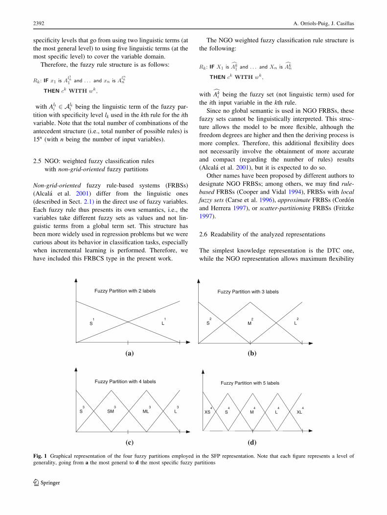
specificity levels that go from using two linguistic terms (at
the most general level) to using five linguistic terms (at the
most specific level) to cover the variable domain.
Therefore, the fuzzy rule structure is as follows:
with Alki 2 A
lki being the linguistic term of the fuzzy par-
tition with specificity level lk used in the kth rule for the ith
variable. Note that the total number of combinations of the
antecedent structure (i.e., total number of possible rules) is
15n (with n being the number of input variables).
2.5 NGO: weighted fuzzy classification rules
with non-grid-oriented fuzzy partitions
Non-grid-oriented fuzzy rule-based systems (FRBSs)
(Alcala et al. 2001) differ from the linguistic ones
(described in Sect. 2.1) in the direct use of fuzzy variables.
Each fuzzy rule thus presents its own semantics, i.e., the
variables take different fuzzy sets as values and not lin-
guistic terms from a global term set. This structure has
been more widely used in regression problems but we were
curious about its behavior in classification tasks, especially
when incremental learning is performed. Therefore, we
have included this FRBCS type in the present work.
The NGO weighted fuzzy classification rule structure is
the following:
with cAki being the fuzzy set (not linguistic term) used for
the ith input variable in the kth rule.
Since no global semantic is used in NGO FRBSs, these
fuzzy sets cannot be linguistically interpreted. This struc-
ture allows the model to be more flexible, although the
freedom degrees are higher and then the deriving process is
more complex. Therefore, this additional flexibility does
not necessarily involve the obtainment of more accurate
and compact (regarding the number of rules) results
(Alcala et al. 2001), but it is expected to do so.
Other names have been proposed by different authors to
designate NGO FRBSs; among others, we may find rule-
based FRBSs (Cooper and Vidal 1994), FRBSs with local
fuzzy sets (Carse et al. 1996), approximate FRBSs (Cordon
and Herrera 1997), or scatter-partitioning FRBSs (Fritzke
1997).
2.6 Readability of the analyzed representations
The simplest knowledge representation is the DTC one,
while the NGO representation allows maximum flexibility
Fuzzy Partition with 2 labels
S1
L1
(a)
Fuzzy Partition with 3 labels
S2
M2
L2
(b)
Fuzzy Partition with 4 labels
S3
SM3
ML3
L3
(c)
Fuzzy Partition with 5 labels
XS4
S4
M4
L4
XL4
(d)
Fig. 1 Graphical representation of the four fuzzy partitions employed in the SFP representation. Note that each figure represents a level of
generality, going from a the most general to d the most specific fuzzy partitions
2392 A. Orriols-Puig, J. Casillas
123

by permitting tuning each individual fuzzy set of each rule,
thus resulting the most complex among the five analyzed
representations.
CNF and SFP lay on a tradeoff between simplicity
and flexibility. Although it is not clearly established
which of the two approaches generates more readable
fuzzy rules, SFP uses a high number of linguistic terms
with different degrees of generality while CNF builds
new fuzzy sets by disjunctions of linguistic terms, so a
clearer meaning is associated to the resulting fuzzy sets
in this latter case. However, the number of possible
disjunctions in CNF will be higher than the number of
fuzzy sets used in SFP when five or more linguistic
terms are considered in the fuzzy partitions of the
former case.
Regarding the standard weighted linguistic fuzzy clas-
sification rule, it will be, in general, more complex than
DTC, CNF and SFP since the whole set of input variables
is used in each rule. The higher the number of variables and
linguistic terms are, the higher the complexity of this
representation will be.
However, interpretability is a sophisticated, subjective,
and controversial concept that sometimes is not ensured by
just generating simple fuzzy rule sets since the explanation
capability may be degraded in these situations (Ishibuchi
et al. 2009).
3 Description of Fuzzy-UCS
Fuzzy-UCS (Orriols-Puig et al. 2009) is a model-free
Michigan-style LFCSs that combine apportionment of
credit techniques and GAs to evolve a population of fuzzy
rules online. In its original definition, Fuzzy-UCS
employed a CNF representation. In what follows, the
integration of the CNF representation into the system and
the learning organization of Fuzzy-UCS are concisely
described. The next section presents the new representa-
tions designed for Fuzzy-UCS.
3.1 Knowledge representation
Fuzzy-UCS evolves a population [P] of classifiers which
together represent the solution to a problem. Each classifier
consists of a rule that follows a CNF representation (see
Sect. 2.3) and a set of parameters. As already mentioned in
the previous section, it is worth noting that this represen-
tation intrinsically permits generalization since each vari-
able can take an arbitrary number of linguistic terms.
In our experiments, all input variables share the same
semantics, which are defined by means of strong fuzzy
partitions that satisfy the equality
X
ni
j¼1
lAijðxÞ ¼ 1; 8xi: ð1Þ
Each partition is a uniformly distributed triangular-shaped
membership function. In our experiments, we used five
linguistic terms.
The matching degree lAkðeÞ of an example e with a
classifier k is computed with the following procedure. For
each variable xi; we compute the membership degree with
each of its linguistic terms, and aggregate them by means
of a T-conorm (disjunction). We enable the system to deal
with missing values by considering that lAkðeiÞ ¼ 1 if the
value ei for the input variable xi is not known. Then, the
matching degree of the rule is determined by the T-norm
(conjunction) of the matching degree of all the input
variables. In our implementation, we used a bounded sum
(minf1; aþ bg) as T-conorm and the product (a � b) as
T-norm. Note that if the fuzzy partition guarantees that the
sum of all membership degrees is greater than or equal to
1—the membership functions employed in our experiments
satisfy this condition—the selected T-norm and T-conorm
allow for a maximum generalization.
Each classifier has four main parameters: (1) the fitness
F, which estimates the accuracy of the rule; (2) the correct
set size ‘cs’, which averages the sizes of the correct sets in
which the classifier has participated (see the next section
for further details on this parameter); (3) the experience
‘exp’, which computes the contributions of the rule to
classify the input instances; and (4) the numerosity ‘num’,
which counts the number of copies of the rule in the
population.
3.2 Organization of the learning process
Fuzzy-UCS repeats the following procedure in order to
evolve a population of maximally general and accurate
rules. At each learning iteration, the system receives an
input example e that belongs to class c. Then, it creates the
match set [M] with all the classifiers in [P] that have a
matching degree lAkðeÞ greater than zero. The following
actions depend on whether the system is in exploitation
(test) mode or exploration (training) mode. In exploitation
mode, the system applies the procedure explained in
Sect. 3.5 to determine the output class; in this case, no
further actions are taken. In exploration mode, the system
takes the following actions in order to improve the pre-
diction of the existing classifiers and to create new prom-
ising ones.
After [M] is constructed, the system builds the correct
set [C] with all the classifiers in [M] that advocate the class
c. If none of the classifiers in [C] match e with the maxi-
mum matching degree, the covering operator is triggered,
Data stream processing and knowledge representation comparison in Fuzzy-UCS 2393
123
which creates the classifier that maximally matches the
input example. In this case, for each variable of the con-
dition, Fuzzy-UCS aggregates the linguistic term Aij that
maximizes the matching degree with the corresponding
input value ei: If ei is not known, a linguistic term is ran-
domly selected and aggregated to the variable. Moreover,
we introduce generalization by allowing the aggregation of
other linguistic terms with probability P#:
The initial values of the parameters of the new classi-
fiers are initialized according to the information provided
by the current examples. Specifically, the fitness, the
numerosity, and the experience are set to 1. The fitness of a
new rule is set to 1 to give it opportunities to take over.
Nonetheless note that, as the new classifiers participate in
new match sets, their fitness and other parameters are
quickly updated to their average values, and so, the initial
value is not crucial. At the end of the covering process, the
new classifier is inserted in the population, deleting another
one if there is no room for it.
3.3 Parameter update
At the end of each learning iteration, Fuzzy-UCS updates
the parameters of the rules that have participated in [M].
First, the experience of the rule is incremented according to
the current matching degree:
expktþ1 ¼ expk
t þ lAkðeÞ ð2Þ
Next, the fitness is updated. For this purpose, each classifier
internally maintains a vector of classes fc1; . . .; cmg; each
of them with an associated weight fvk1; . . .; vk
mg: Each
weight vkj indicates the soundness with which rule k pre-
dicts class j for an example that fully matches this rule.
These weights are incrementally updated during learning
by the following procedure.
We first compute these sum of correct matchings cmk
for each class j:
cmkjtþ1¼ cmk
jtþ mðk; jÞ; ð3Þ
where
mðk; jÞ ¼ lAkðeÞ if j ¼ c;0 otherwise.
�
ð4Þ
Then, cmkjþ1 is used to compute the weights vk
jþ1 :
8j : vkjtþ1¼
cmkjtþ1
expktþ1
: ð5Þ
For example, if a rule k only matches examples of class j,
the weight vkj will be 1 and the remaining weights 0. Rules
that match instances of both classes will have weights
ranging from 0 to 1. Note that the sum of all the weights
is 1.
The fitness is then computed from the weights with the
aim of favoring classifiers that match examples of a single
class. To carry this out, we use the following formula
(Ishibuchi and Yamamoto 2005):
Fktþ1 ¼ vk
maxtþ1�X
jjj 6¼max
vkjtþ1; ð6Þ
where we subtract the values of the other weights from the
weight with maximum value vkmax: The fitness Fk is the
value used as the weight wk of the rule. Note that this
formula can result in classifiers with zero or negative fit-
ness (e.g., if the number of classes is greater than 2 and the
class weights are equal). Next, the correct set size of all the
classifiers in [C] is calculated as the arithmetic average of
the sizes of all the correct sets in which the classifier has
participated.
Finally, the rule k predicts the class c with the highest
weight associated vkc: Thus, the class predicted is not fixed
when the rule is created, and it can change as the param-
eters of the rule are updated (especially during the first
parameter updates).
3.4 Discovery component
Fuzzy-UCS uses a steady-state niche-based GA (Goldberg
2002) to discover new promising rules. The GA is applied
to the [C] activated in the current iteration. Thus, the
niching is intrinsically provided since the GA is applied to
rules that match the same input with a degree greater than
zero and advocate the same class.
The GA is triggered when the average time from its last
application upon the classifiers in [C] exceeds the threshold
hGA: It selects two parents p1 and p2 from [C] using tour-
nament selection (Butz et al. 2005). The two parents are
copied into offspring ch1 and ch2; which undergo crossover
and mutation with probabilities v and l; respectively. The
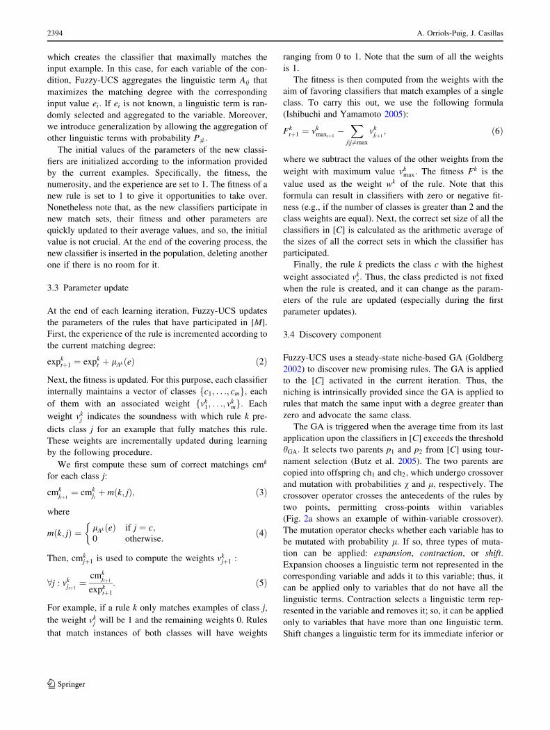
crossover operator crosses the antecedents of the rules by
two points, permitting cross-points within variables
(Fig. 2a shows an example of within-variable crossover).
The mutation operator checks whether each variable has to
be mutated with probability l: If so, three types of muta-
tion can be applied: expansion, contraction, or shift.
Expansion chooses a linguistic term not represented in the
corresponding variable and adds it to this variable; thus, it
can be applied only to variables that do not have all the
linguistic terms. Contraction selects a linguistic term rep-
resented in the variable and removes it; so, it can be applied
only to variables that have more than one linguistic term.
Shift changes a linguistic term for its immediate inferior or
2394 A. Orriols-Puig, J. Casillas
123
superior. An example of each type of mutation is illustrated
in Fig. 2b.
The new offspring are introduced into the population.
First, each classifier is checked for subsumption (Wilson
1998) with their parents. That is, if any parent’s condition
subsumes the condition of the offspring (i.e., the parent
has, at least, the same linguistic terms per variable as the
child), and this parent is highly accurate (Fk [ F0) and
sufficiently experienced (expk [ hsub), the offspring is not
inserted and the numerosity of the parent is increased by
one. Note that F0 and hsub are configuration parameters.
Otherwise, we check [C] for the most general rule that can
subsume the offspring. If no subsumer can be found, the
classifier is inserted in the population.
If the population is full, excess classifiers are deleted
from [P] with probability proportional to the correct set
size estimate ‘cs’. Moreover, if the classifier is sufficiently
experienced (expk [ hdel) and the power of its fitness ðFkÞm
is significantly lower than the average fitness of the clas-
sifiers in [P] ððFkÞm\dF½P� where F½P� ¼ 1N
P
i2½P�ðFiÞmÞ, its
deletion probability is further increased. That is, each
classifier has a deletion probability pk of:
pk ¼dk
P
8j2½P� dj; ð7Þ
where
dk ¼cs�num�F½P�ðFkÞm if expk [ hdel and ðFkÞm\dF½P�;
cs � num otherwise.
�
ð8Þ
Thus, the deletion algorithm balances the classifier allo-
cation in the different correct sets by pushing toward
deletion of rules belonging to large correct sets. At the
same time, it favors the search toward highly fit classifiers,
since the deletion probability of rules whose fitness is much
smaller than the average fitness is increased.
Parent2Parent1
Child2Child1
Crossover
IF X 1 is THEN A 1 IF X 1 is THEN A 2
IF X 1 is THEN A 2 IF X 1 is THEN A 1
(a)
noitcartnoCnoisnapxE Shift
Mutation
IF X 1 is THEN A 1
IF X 1 is IF X 1 isTHEN A 1 THEN A 1 THEN A 1IF X 1 is
(b)
Fig. 2 Graphical example of
a crossover and b mutation for
the CNF representation
Data stream processing and knowledge representation comparison in Fuzzy-UCS 2395
123

3.5 Class inference in test mode
To decide the predicted class given an input instance, all
the experienced rules vote for the class they predict. Each
rule k emits a vote vk for the class it advocates, where
vk ¼ Fk � lAkðeÞ: The votes for each class j are added:
8j : votej ¼X
N
kjck¼j
vk; ð9Þ
and the most-voted class is returned as the output.
4 New representations for Fuzzy-UCS
This section shows how we have integrated the three rep-
resentations explained in Sect. 2, in addition to the CNF
representation introduced in the last section, to Fuzzy-
UCS. For each representation, we explain how the process
organization of Fuzzy-UCS has been modified to let the
system deal with the new types of rules.
4.1 DTC representation
In the DTC representation (Sect. 2.2), a variable can take
either (1) a single linguistic term or (2) a don’t care value.
To adapt Fuzzy-UCS to this new type of fuzzy rules, we
modified the following operators with the aim of avoiding
the creation of rules that contain variables with more than
one linguistic term.
4.1.1 Covering operator
As in the original CNF approach, when triggered, the
covering operator creates the classifier that best matches
the input example. However, the generalization procedure
is modified. Now, each variable is set to don’t care with
probability P#:
4.1.2 Crossover operator
We apply a two-point crossover operator as in the CNF
approach. However, in this case, we only allow selecting
crossing points between variables to avoid the creation of
children with variables that contain either zero or multiple
linguistic terms.
4.1.3 Mutation operator
Three types of mutation can be applied depending on the
variable selected. If the variable is represented by a don’t
care, a linguistic term is randomly selected and set to the
variable. If the variable is represented by a linguistic term,
mutation either (1) sets the variable to don’t care with
probability Pl# or (2) replaces the linguistic term with its
immediate superior or inferior by applying the shift oper-
ators of Fuzzy-UCS with the CNF representation.
4.2 SFP representation
Similar to the DTC representation, in the SFP representa-
tion, each variable can take a single linguistic term or a
don’t care value. However, the SFP representation pro-
vides the system with a richer set of labels using fuzzy
partitions of different granularities that enable moving
from generality to specificity. The modifications introduced
to deal with this representation are explained as follows.
4.2.1 Covering operator
The same approach used in the DTC representation is
employed here. Therefore, the covering operator creates
the classifier that best matches the input instance; i.e., for
each variable, it selects the linguistic term that maximizes
the matching degree with the corresponding input value.
Besides, each variable is set to don’t care with probability
P#.
4.2.2 Crossover operator
We apply two-point crossover, only allowing cut points
between variables.
4.2.3 Mutation operator
When applied, the mutation operator changes the linguistic
term assigned to the variable so that either (1) a more
general or more specific linguistic term is used or (2) its
level of specificity remains equal but it is replaced with one
of its adjacent linguistic terms. More specifically, the fol-
lowing procedure is applied:
• If the variable is represented by a don’t care, a
linguistic term of any of the four fuzzy partitions is
randomly assigned to the variable.
• If the variable is represented by a linguistic term, we
randomly select whether the linguistic term should (1)
become more general, (2) more specific, or (3) keep the
same degree of generality. In the first two cases, a
linguistic term of the fuzzy partition with one less
number of terms or with one more number of terms is
randomly selected among those that intersect with the
linguistic term currently assigned to the variable. In the
third case, one of the neighbors of the current linguistic
term of the same fuzzy partition is selected and used to
replace the current one.
2396 A. Orriols-Puig, J. Casillas
123

4.3 NGO representation
While in the three previous representations the same
semantics was shared among all the variables in the fuzzy
rule base, the NGO representation enables using an inde-
pendent fuzzy set for each variable of each rule. In our
experiments, we used triangular-shaped fuzzy sets. There-
fore, each variable’s rule is represented by three continuous
values ak; bk; and ck; which, respectively, represent the left
vertex, the middle vertex, and the right vertex of the tri-
angular fuzzy set. Then, the evolutionary process is
responsible for tuning the fuzzy sets of each variable’s rule.
The modifications introduced to deal with this representa-
tion are elaborated as follows.
4.3.1 Covering operator
As in the previous representations, the covering operator
creates the classifier that best matches the input example,
allowing a certain amount of generalization. To simulate
the same approach, given the input example e that has
caused covering to trigger, the operator creates an inde-
pendent triangular-shaped fuzzy set for each input variable
with the following supports
rand mini �maxi �mini
2; ei
� �
; ei;
�
rand ei;maxi þmaxi �mini
2
� ��
ð10Þ
where mini and maxi are the minimum and maximum value
that the ith attribute can take, ei is the ith attribute of the
example e for which covering has been fired, and rand
generates a random number between both arguments.
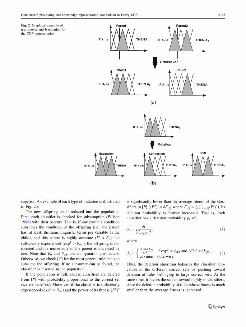
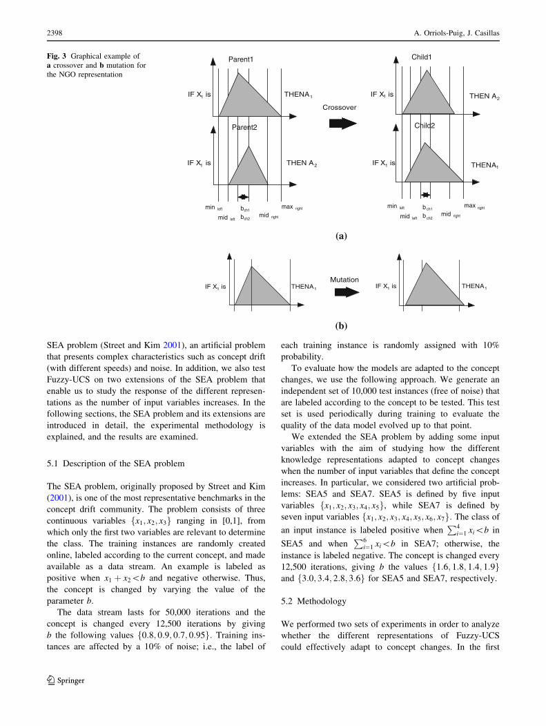
4.3.2 Crossover operator
The crossover operator generates the fuzzy sets for each
variable of the offspring as
bch1¼ bp1
� aþ bp2� ð1� aÞ and ð11Þ
bch2¼ bp1
� ð1� aÞ þ bp2� a; ð12Þ
where 0� a� 1 is a configuration parameter. As we want
to generate offspring whose middle vertex b is close to the
middle vertex of one of his parents, we set a ¼ 0:005 in our
experiments. Next, for both offspring, the procedure to
cross the most-left and most-right vertices is the following.
First, the two most-left and two most-right vertices are
chosen
minleft ¼ minðap1; ap2
; bchÞ and ð13Þ
midleft ¼ middleðap1; ap2
; bchÞ; ð14Þ
midright ¼ middleðcp1; cp2
; bchÞ and ð15Þ
maxright ¼ maxðcp1; cp2
; bchÞ: ð16Þ
And then, these two values are used to generate the vertices
a and c.
ach ¼ randðminleft;midleftÞ and ð17Þcch ¼ randðmidright;maxrightÞ; ð18Þ
where the functions ‘min’, ‘middle’, and ‘max’ return,
respectively, the minimum, the middle, and the maximum
values among their arguments. Figure 3a shows an exam-
ple of crossover.
4.3.3 Mutation operator
The mutation operator decides randomly if each vertex of a
variable has to be mutated. The central vertex is mutated as
follows:
bk ¼ randðbk � ðbk � akÞ � m0; bk þ ðck � bkÞ � m0Þ ð19Þ
where m0 (0\m0� 1) defines the strength of the mutation.
The left-most vertex is mutated as
ak ¼rand ak � bk�ak
2m0; ak
� �
if F [ F0 and no cross.
rand ak � bk�ak
2m0; ak þ bk�ak
2m0
� �
otherwise:
�
ð20Þ
And the right-most vertex
ck ¼rand ck; ck þ ck�bk
2m0
� �
if F [ F0 and no cross.
rand ck � ck�bk
2m0; ck þ ck�bk
2m0
� �
otherwise:
�
ð21Þ
That is, if the rule is accurate enough (F [ F0) and has not
been generated through crossover, mutation forces to
generalize it. Otherwise, it can be either generalized or
specified. In this way, we increase the pressure toward
maximum general and accurate rule sets. Figure 3b shows
an example of mutation.
Thus far, we have explained the learning process of
Fuzzy-UCS with four different types of representations that
move through the dimensions of flexibility and simplicity
(see Sect. 2.6). With these descriptions in mind, we now
are in position to start analyzing how the different repre-
sentations perform in (1) data streams with concept chan-
ges and (2) real-world problems extracted from public
repositories. These analyses are conducted in the sub-
sequent sections.
5 Experiments on problems with concept changes
This section analyzes how Fuzzy-UCS adapts to data
streams where concepts change over time, and compares
the system to some of the most significant methods in the
data stream mining field. For this purpose, we first use the
Data stream processing and knowledge representation comparison in Fuzzy-UCS 2397
123
SEA problem (Street and Kim 2001), an artificial problem
that presents complex characteristics such as concept drift
(with different speeds) and noise. In addition, we also test
Fuzzy-UCS on two extensions of the SEA problem that
enable us to study the response of the different represen-
tations as the number of input variables increases. In the
following sections, the SEA problem and its extensions are
introduced in detail, the experimental methodology is
explained, and the results are examined.
5.1 Description of the SEA problem
The SEA problem, originally proposed by Street and Kim
(2001), is one of the most representative benchmarks in the
concept drift community. The problem consists of three
continuous variables fx1; x2; x3g ranging in [0,1], from
which only the first two variables are relevant to determine
the class. The training instances are randomly created
online, labeled according to the current concept, and made
available as a data stream. An example is labeled as
positive when x1 þ x2\b and negative otherwise. Thus,
the concept is changed by varying the value of the
parameter b.
The data stream lasts for 50,000 iterations and the
concept is changed every 12,500 iterations by giving
b the following values f0:8; 0:9; 0:7; 0:95g: Training ins-
tances are affected by a 10% of noise; i.e., the label of
each training instance is randomly assigned with 10%
probability.
To evaluate how the models are adapted to the concept
changes, we use the following approach. We generate an
independent set of 10,000 test instances (free of noise) that
are labeled according to the concept to be tested. This test
set is used periodically during training to evaluate the
quality of the data model evolved up to that point.
We extended the SEA problem by adding some input
variables with the aim of studying how the different
knowledge representations adapted to concept changes
when the number of input variables that define the concept
increases. In particular, we considered two artificial prob-
lems: SEA5 and SEA7. SEA5 is defined by five input
variables fx1; x2; x3; x4; x5g, while SEA7 is defined by
seven input variables fx1; x2; x3; x4; x5; x6; x7g: The class of
an input instance is labeled positive whenP4
i¼1 xi\b in
SEA5 and whenP6
i¼1 xi\b in SEA7; otherwise, the
instance is labeled negative. The concept is changed every
12,500 iterations, giving b the values f1:6; 1:8; 1:4; 1:9gand f3:0; 3:4; 2:8; 3:6g for SEA5 and SEA7, respectively.
5.2 Methodology
We performed two sets of experiments in order to analyze
whether the different representations of Fuzzy-UCS
could effectively adapt to concept changes. In the first
Parent1
Parent2
bch1
bch2
min left max right
mid rightmid left
Child1
Child2
b ch1
b ch2
min left max right
mid rightmid left
Crossover
IF X 1 is THEN A 1 IF X 1 is THEN A 2
IF X 1 is THEN A 2 IF X 1 is THEN A 1
(a)
MutationIF X 1 is THEN A 1 IF X 1 is THEN A 1
(b)
Fig. 3 Graphical example of
a crossover and b mutation for
the NGO representation
2398 A. Orriols-Puig, J. Casillas
123

experiment, we compared Fuzzy-UCS with the four rule
representations with other competitive learning systems
prepared to deal with data streams on the SEA problem. In
particular, we considered IBk (Aha et al. 1991) with k = 1
and a global window of 12,500, as employed by Nunez
et al. (2007),2 and OnlineTree2 (Nunez et al. 2007), a
decision tree specifically designed to deal with data streams
that have been shown to significantly outperform the state-
of-the-art algorithms in the data stream mining realm. IBk
was run by adapting the implementation provided in Weka
(Witten and Frank 2005). The results of OnlineTree2 were
those presented in Nunez et al. (2007), which were kindly
provided by the authors.
In the second experiment, we analyzed how the increase
in the number of input variables that defined the problem
concept affected the behavior of the different representa-
tions. For this purpose, we ran Fuzzy-UCS with the four
representations on the SEA5 and SEA7 problems. In this
case, only the results obtained with IBk were included,
since results of OnlineTree2 were not available for these
two problems in Nunez et al. (2007).
For all the representations, Fuzzy-UCS was configured
with the following parameters: acc0 ¼ 0:99; m ¼ 5; hGA ¼25; hdel ¼ 20; hsub ¼ 50; hexploit ¼ 10; d ¼ 0:1; and P# ¼0:20: The population size was set to 1,000, 2,000, and
4,000 in the SEA, SEA5 and SEA6 problems, respectively.
We used tournament selection with r ¼ 0:4: Crossover and
mutation were applied with probabilities 0.8 and 0:5=‘;
where ‘ is the number of input variables of the problem.
For the DTC representation, Pl# ¼ 0:25: The error of the
model being evolved was evaluated every 500 iterations
with the test set. All the runs for each representation were
repeated with 10 different random seeds, and the results
provided are averages of these runs.
The results were statistically compared following the
recommendations pointed out by Demsar (2006). Thus, in all
the analyses, we used non-parametric statistical tests to
compare the results obtained by the different techniques. We
first applied multiple-comparison statistical procedures to
test the null hypothesis that all the learning algorithms per-
formed equivalently on average. Specifically, we used the
Friedman’s test (Friedman 1937, 1940). If the Friedman’s
test rejected the null hypothesis, we used the non-parametric
Nemenyi’s test (Nemenyi 1963) to compare all learners to
each other. The Nemenyi’s test defines that two methods are
significantly different if the corresponding average rank
differs by at least a critical difference CD computed as
CD ¼ qa
ffiffiffiffiffiffiffiffiffiffiffiffiffiffiffiffiffiffiffiffi
n‘ðn‘ þ 1Þ6nds
s
; ð22Þ
where n‘ and nds are the number of learners and the number
of performance measurements, and qa is the critical value
based on the Studentized range statistic (Sheskin 2000).
To complement the multi-comparison statistical analy-
sis, we performed pairwise comparisons by means of the
Holm’s step-down procedure and the Shaffer’s test as
recommended by Garcıa and Herrera (2008). These sta-
tistical procedures consider the interrelation of each pair-
wise comparison that comes from a multiple learner
comparison to adjust the significance level of each pairwise
comparison. To run these tests, we used the open-source
code that can be downloaded from the author’s webpage.3
5.3 Analysis of Fuzzy-UCS on the SEA problem
Figure 4 shows the evolution of the test error obtained
with the four representations of Fuzzy-UCS, IBk, and
0.000
0.025
0.050
0.075
0.100
0.125
0.150
0.175
0.200
0.225
0.250
0 12500 25000 37500 50000
erro
r
iteration
NGOSFPCNFDTC
IBkOnlineTree2
Fig. 4 Comparison of the test error achieved by Fuzzy-UCS, with each rule representation, IBk, and OnlineTree2 on the SEA problem. Every
12,500 iterations, the concept of the problem changes, causing a concept drift
2 Note the size of the window selected permits storing all the
examples sampled for a specific concept; therefore, we would expect
an optimal behavior of IBk after having seen 12,500 examples of the
same concept. 3 http://sci2s.ugr.es/sicidm/multipleTest.zip.
Data stream processing and knowledge representation comparison in Fuzzy-UCS 2399
123
OnlineTree2. The Friedman’s test rejected the null
hypothesis that the four representations of Fuzzy-UCS,
IBk, and OnlineTree2 performed the same on average with
p value almost equal to zero. Therefore, we applied the
Nemenyi’s test, whose results are summarized in Fig. 5. In
order to provide a detailed analysis, we compared the
performance obtained by the six methods (1) on the whole
run and (2) on each one of the four concepts that are
sampled during a run of the SEA problem. The statistical
analysis is complemented in Table 1, where the results of
the pairwise comparisons following the Holm’s and the
Shaffer’s procedures are illustrated. In this case, note that
we can reject the null hypothesis that two learners per-
formed the same on average when the p value is lower than
the corresponding a value adjusted by the Holm’s and the
Shaffer’s procedure, respectively (two last columns of the
table). Pairwise comparisons for which the null hypothesis
could be rejected are marked in bold. The conclusions and
comments extracted from these results are summarized in
what follows.
The results in Fig. 4 illustrate a common behavior when
the system faces a concept drift: all the error curves sud-
denly rocketed. Obviously, this happened because the data
models had been built from examples that represented the
previous concept. The systems more affected by concept
changes were IBk and OnlineTree2, whose error presented
the highest increases in almost all the concept changes.
The most interesting part though is the shape of the
curves from each concept change, since it shows the
reaction capacity of each method. IBk presented a linear
recovery to the average error rate, which decreased until
approximately 8% of error in all the four concepts. Note
that this error was close to the 10% noise added to the
problem. With no doubt, IBk had the worst reaction
capacity. OnlineTree2 had a much quicker recovery time to
the average error rate, which ended around 2.5% at the end
of each concept. The excellent results obtained by
OnlineTree2 are not surprising, since it has been empirically
demonstrated to be one of the most accurate data stream
miners (Nunez et al. 2007). On the other hand, all the
representations of Fuzzy-UCS presented a quick recovery
to the average error rate, which was similar in shape to that
of OnlineTree2. Fuzzy-UCS reached the end of each con-
cept with errors that ranged between 2.4 and 6% depending
on the representation used and concept learned. Notice two
important issues here. First, the error achieved with the
different representations of Fuzzy-UCS was lower than the
10% error added to the system, which indicates that Fuzzy-
UCS is robust to noise. Second, the reaction capacity of
Fuzzy-UCS was much better than those of IBk and of
OnlineTree2. It is worth noting that the concept changes
affected the different representations of Fuzzy-UCS to a
lower extend than IBk and especially than OnlineTree2.
Consequently, the models of Fuzzy-UCS were more
accurate than those of OnlineTree2 the majority of the
time. If we specifically focus on Fuzzy-UCS with the NGO
representation, we can observe that the models evolved by
Fuzzy-UCS were more accurate than those created by
OnlineTree2 almost all the time and that the error reached
at the end of each concept was approximately the same.
Thus, Fuzzy-UCS—especially the NGO representation—
was more robust to concept changes and had a faster
adaptation to the new concepts than IBk and OnlineTree2.
A closer look to the statistical analysis illustrated in
Fig. 5 enables extending the conclusions about the per-
formance of the different systems. Considering the whole
run (see G row in Fig. 5), we can see that Fuzzy-UCS with
0 2 4 6 8
G
C1
C2
C3
C4
NGO
SFP
CNF
DTC
OnlineTree2
IBk
NGO
SFP
CNF
DTC
OnlineTree2
IBk
NGO
SFP
CNF
DTC
OnlineTree2
IBk
NGO
SFP
CNF
DTC
OnlineTree2
IBk
NGO
SFP
CNF
DTC
OnlineTree2
IBk
Rank
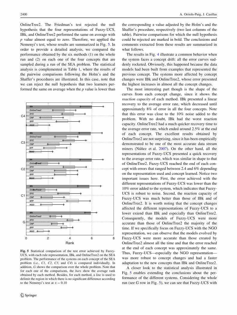
Fig. 5 Statistical comparison of the test error achieved by Fuzzy-
UCS, with each rule representation, IBk, and OnlineTree2 on the SEA
problem. The performance of the systems on each concept of the SEA
problem (i.e., C1, C2, C3, and C4) is compared individually. In
addition, G shows the comparison over the whole problem. Note that
for each one of the comparisons, the bars show the average rank
obtained by each method. Besides, for each method, a line is used to
delimit the region in which there is no significant difference according
to the Nemenyi’s test at a ¼ 0:10
2400 A. Orriols-Puig, J. Casillas
123
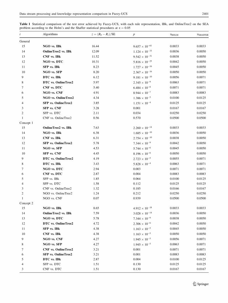
Table 1 Statistical comparison of the test error achieved by Fuzzy-UCS, with each rule representation, IBk, and OnlineTree2 on the SEA
problem according to the Holm’s and the Shaffer statistical procedures at a ¼ 0:05
i Algorithms z ¼ ðR0 � RiÞ=SE p aHOLM aSHAFFER
General
15 NGO vs. IBk 16.44 9:657� 10�61 0.0033 0.0033
14 OnlineTree2 vs. IBk 12.09 1:124� 10�33 0.0036 0.0050
13 CNF vs. IBk 11.52 9:542� 10�31 0.0038 0.0050
12 NGO vs. DTC 10.31 5:816� 10�25 0.0042 0.0050
11 SFP vs. IBk 8.23 1:727� 10�16 0.0045 0.0050
10 NGO vs. SFP 8.20 2:367� 10�16 0.0050 0.0050
9 DTC vs. IBk 6.12 9:181� 10�10 0.0056 0.0071
8 DTC vs. OnlineTree2 5.97 2:345� 10�9 0.0063 0.0071
7 CNF vs. DTC 5.40 6:484� 10�8 0.0071 0.0071
6 NGO vs. CNF 4.91 8:944� 10�7 0.0083 0.0083
5 NGO vs. OnlineTree2 4.34 1:386� 10�5 0.0100 0.0125
4 SFP vs. OnlineTree2 3.85 1:151� 10�4 0.0125 0.0125
3 SFP vs. CNF 3.28 0.001 0.0167 0.0167
2 SFP vs. DTC 2.11 0.034 0.0250 0.0250
1 CNF vs. OnlineTree2 0.56 0.570 0.0500 0.0500
Concept 1
15 OnlineTree2 vs. IBk 7.63 2:260� 10�14 0.0033 0.0033
14 NGO vs. IBk 6.38 1:685� 10�10 0.0036 0.0050
13 CNF vs. IBk 6.31 2:754� 10�10 0.0038 0.0050
12 SFP vs. OnlineTree2 5.78 7:344� 10�9 0.0042 0.0050
11 NGO vs. SFP 4.53 5:744� 10�6 0.0045 0.0050
10 SFP vs. CNF 4.45 8:196� 10�6 0.0050 0.0050
9 DTC vs. OnlineTree2 4.19 2:723� 10�5 0.0055 0.0071
8 DTC vs. IBk 3.43 5:828� 10�4 0.0063 0.0071
7 NGO vs. DTC 2.94 0.003 0.0071 0.0071
6 CNF vs. DTC 2.87 0.004 0.0083 0.0083
5 SFP vs. IBk 1.85 0.064 0.0100 0.0125
4 SFP vs. DTC 1.58 0.112 0.0125 0.0125
3 CNF vs. OnlineTree2 1.32 0.185 0.0166 0.0167
2 NGO vs. OnlineTree2 1.24 0.212 0.0250 0.0250
1 NGO vs. CNF 0.07 0.939 0.0500 0.0500
Concept 2
15 NGO vs. IBk 8.65 4:912� 10�18 0.0033 0.0033
14 OnlineTree2 vs. IBk 7.59 3:028� 10�14 0.0036 0.0050
13 NGO vs. DTC 5.78 7:344� 10�9 0.0038 0.0050
12 DTC vs. OnlineTree2 4.72 2:306� 10�6 0.0042 0.0050
11 SFP vs. IBk 4.38 1:163� 10�5 0.0045 0.0050
10 CNF vs. IBk 4.38 1:163� 10�5 0.0050 0.0050
9 NGO vs. CNF 4.27 1:945� 10�5 0.0056 0.0071
8 NGO vs. SFP 4.27 1:945� 10�5 0.0063 0.0071
7 CNF vs. OnlineTree2 3.21 0.001 0.0071 0.0071
6 SFP vs. OnlineTree2 3.21 0.001 0.0083 0.0083
5 DTC vs. IBk 2.87 0.004 0.0100 0.0125
4 SFP vs. DTC 1.51 0.130 0.0125 0.0125
3 CNF vs. DTC 1.51 0.130 0.0167 0.0167
Data stream processing and knowledge representation comparison in Fuzzy-UCS 2401
123

the NGO representation significantly outperformed all the
other methods, including OnlineTree2 and the remaining
representations of Fuzzy-UCS, according to the Nemenyi’s
test at a ¼ 0:10: The next best systems in the comparison
were OnlineTree2 and Fuzzy-UCS with the CNF repre-
sentation, which significantly outperformed the other
two representations of Fuzzy-UCS and IBk. The SFP rep-
resentation obtained significantly better results than the
DTC one and IBk resulted in the poorest results, being
significantly outperformed by all the other systems. These
results were confirmed by the Holm’s and the Shaffer’s
procedures illustrated in Table 1, with the exception that
they did not identify any significant difference between the
DTC and the SFP representations of Fuzzy-UCS.
The ranking of the representations of Fuzzy-UCS was
expected since the significantly best results were obtained
with those representations that are more flexible. That is,
the NGO representation allows the creation of individual
Table 1 continued
i Algorithms z ¼ ðR0 � RiÞ=SE p aHOLM aSHAFFER
2 NGO vs. OnlineTree2 1.05 0.289 0.0250 0.0250
1 SFP vs. CNF 0.00 0.999 0.0500 0.0500
Concept 3
15 NGO vs. IBk 8.54 1:319� 10�17 0.0033 0.0033
14 SFP vs. IBk 6.08 1:163� 10�9 0.0036 0.0050
13 NGO vs. DTC 5.78 7:344� 10�9 0.0038 0.0050
12 CNF vs. IBk 5.40 6:484� 10�8 0.0042 0.0050
11 NGO vs. OnlineTree2 4.34 1:382� 10�5 0.0045 0.0050
10 OnlineTree2 vs. IBk 4.19 2:723� 10�5 0.0050 0.0050
9 SFP vs. DTC 3.32 8:807� 10�4 0.0055 0.0071
8 NGO vs. CNF 3.13 0.001 0.0063 0.0071
7 DTC vs. IBk 2.75 0.005 0.0071 0.0071
6 CNF vs. DTC 2.64 0.008 0.0083 0.0083
5 NGO vs. SFP 2.45 0.014 0.0100 0.0125
4 SFP vs. OnlineTree2 1.88 0.058 0.0125 0.0125
3 DTC vs. OnlineTree2 1.43 0.150 0.0167 0.0167
2 CNF vs. OnlineTree2 1.20 0.226 0.0250 0.0250
1 SFP vs. CNF 0.68 0.496 0.0500 0.0500
Concept 4
15 NGO vs. IBk 9.29 1:432� 10�20 0.0033 0.0033
14 CNF vs. IBk 6.95 3:536� 10�12 0.0036 0.0050
13 NGO vs. DTC 6.12 9:181� 10�10 0.0038 0.0050
12 NGO vs. SFP 5.14 2:742� 10�7 0.0042 0.0050
11 OnlineTree2 vs. IBk 4.76 1:913� 10�6 0.0045 0.0050
10 NGO vs. OnlineTree2 4.53 5:744� 10�6 0.0050 0.0050
9 SFP vs. IBk 4.15 3:215� 10�5 0.0055 0.0071
8 CNF vs. DTC 3.77 1:570� 10�4 0.0063 0.0071
7 DTC vs. IBk 3.17 0.001 0.0071 0.0071
6 SFP vs. CNF 2.79 0.005 0.0083 0.0083
5 NGO vs. CNF 2.34 0.019 0.0100 0.0125
4 CNF vs. OnlineTree2 2.19 0.028 0.0125 0.0125
3 DTC vs. OnlineTree2 1.58 0.112 0.0167 0.0167
2 SFP vs. DTC 0.98 0.325 0.0250 0.0250
1 SFP vs. OnlineTree2 0.60 0.545 0.0500 0.0500
First, the performance of the six methods over the whole run is compared, and then the performance of the systems on each concept of the SEA
problem is compared individually. For each comparison, the columns show the comparison number, the algorithms compared, the test statistics z,
the adjustment of a by Holm’s procedure (aHOLM), and the adjustment of a by Shaffer’s procedure (aSHAFFER). Methods that perform significantly
different according to both the Holm’s and the Shaffer’s test are marked in bold
2402 A. Orriols-Puig, J. Casillas
123

triangular-shaped fuzzy sets for each variable, enabling a
high flexibility. Therefore, it was expected that this repre-
sentation permitted fitting the class boundaries more
accurately than the remaining ones. The CNF representa-
tion assigns a disjunction of linguistic terms to each vari-
able; so, although it is not as flexible as the NGO
representation, the aggregation of these terms can result in
fuzzy sets of different shape which may be useful to fit
complex class boundaries. The results confirmed this
hypothesis, illustrating that the CNF representation resulted
in models that were significantly poorer than those
obtained by the NGO representation, but significantly more
accurate than those created with the other two representa-
tions. The last two representations in the statistical analysis
were the SFP and the DTC ones. Both representations
assign a single linguistic term to each variable or a don’t care
symbol. Therefore, these two representations are not as
flexible as the former ones. Note that the SFP representation
led to significantly better results that the DTC one, since
its semantics consists of a higher number of linguistic
terms, organized in a hierarchy that enables moving through
the specificity-generality dimension more quickly.
A closer inspection of the statistical analysis provided in
the rows C1, C2, C3, and C4 of Fig. 5 and in Table 1 lets
us point out more aspects of the performance and reaction
capacity of the different representations of Fuzzy-UCS and
OnlineTree2 on each concept of the SEA problem sepa-
rately. In the following discussion, we put IBk aside, since
it achieved the worst results in all the concepts. The NGO
representation was the best ranked in the concepts C2, C3,
and C4. In the remaining concept, C2, it was the second
best ranked, after OnlineTree2. This indicates that, as
pointed out above, the NGO representation could react
quickly to concept changes. It is worth mentioning that
OnlineTree2 could reach similar errors, and in some cases
even better, to those of the NGO representation; however,
OnlineTree2 was deeply affected by the concept change
and needed much more time to recover. The CNF repre-
sentation was the third best ranked in C1 (obtaining sta-
tistically equivalent results to those of the NGO
representation and OnlineTree2), C2 and C3; and it was the
second best ranked in C4. The SFP representation pre-
sented very different behaviors on the diverse concepts. It
was the second best ranked in C3, the fourth best ranked in
C2 and C4, and the fifth best ranked in C1. Finally, the
DTC representation presented the worst results, being
the poorest ranked in concepts C2, C3, and C4 (i.e., all the
concepts that come after a concept change), and was
ranked fourth in concept C1. The curves in Fig. 4—espe-
cially, the flat decrease shown in concepts C2 and C4—
support the hypothesis that the high generality pressure
supplied by this representation hampers it from fitting the
class boundary more accurately.
5.4 Effect of increasing the number of input variables
Having extensively analyzed the behavior of the four rep-
resentations on the SEA problem, this section analyzes how
the number of input variables affects the performance of
the different representations. Intuitively, on the one hand,
less flexible representations may suffer when approaching
more complex class boundaries. On the other hand, the
reaction time may increase in all the representations, but
especially on those that offer more flexibility. To check
these hypotheses, we ran Fuzzy-UCS on the SEA5 and
SEA7 problems. Figures 6 and 7 show the evolution of the
test error of Fuzzy-UCS and IBk in the two problems.
Figure 8 and Table 2 supply the results of the Nemenyi’s
and the Holm’s and Shaffer’s tests, respectively. In what
follows, we point out two important observations drawn
from these results.
First, the results indicate that Fuzzy-UCS with the four
representations had more difficulties to learn the different
subconcepts of the SEA5 and SEA7 problems than those
0.0000.0250.0500.0750.1000.1250.1500.1750.2000.2250.2500.2750.3000.3250.350
0 12500 25000 37500 50000
erro
r
iteration
NGOSFPCNFDTC
IBk
Fig. 6 Comparison of the test error achieved by Fuzzy-UCS, with each rule representation, and IBk on the SEA5 problem. Every 12,500
iterations, the concept of the problem changes, causing a concept drift
Data stream processing and knowledge representation comparison in Fuzzy-UCS 2403
123

observed in the SEA problem. That is, while Fuzzy-UCS
could achieve errors close to 0.025 in all the subconcepts of
the SEA problem (see Fig. 4), the system resulted in errors
higher that 0.05 in some of the subconcepts of the SEA5
and SEA7 problems. This behavior was expected since
both SEA5 and SEA7 are more complex than the original
SEA problem. That is, SEA5 and SEA7 require that rules
consider four and six input variables to accurately deter-
mine the output, while only two variables have to be
considered in the SEA problem. Besides, the oblique class
boundary of the problems requires a high number of rules
that accurately approximate it. For this reason, a higher test
error concentrated on the class boundary. In particular, the
error presented by the DTC and SFP representations was
specifically high in some specific subconcepts, which
indicates that the lower flexibility provided by these rep-
resentations may not be enough to accurately approximate
the class boundary in complex subconcepts. Nevertheless,
it is worth highlighting that Fuzzy-UCS with any repre-
sentation still significantly outperformed IBk on the SEA7
problem according to the Holm’s and Shaffer’s procedures at
a ¼ 0:05: Fuzzy-UCS with NGO and CNF representation
also significantly outperformed IBk on the SEA5 problem.
Second, Figs. 6 and 7 show that Fuzzy-UCS with the
two most flexible representations—i.e., NGO and CNF—
obtained the best results overall. This aligns with the
observations made in the SEA problem, since the flexibility
of both representations enabled Fuzzy-UCS to quickly
react to concept changes and approximate the new concept
in the SEA5 and SEA7 problems as well. The most inter-
esting results though are reported in Fig. 7. Note that
although NGO was not outperformed by CNF during all the
run, CNF permitted the system to achieve better accuracies
than NGO in three of the four subconcepts. We hypothesize
that this is due to the high flexibility provided by NGO,
which may have hindered the system from fully adapting to
new concepts as the system needed to tune the vertices of
the fuzzy rules for each rule variable, thus resulting in a
huge search space. On the other hand, CNF also provides
good flexibility but resulting in a smaller search spaces,
allowing the system to adapt to changes more quickly.
The overall study conducted in this section has served to
confirm that Fuzzy-UCS is a very robust and competitive
system to deal with data streams that present concept drift,
which was defined as the first objective of this work. The
experimental evidence has highlighted that all the four
representations of Fuzzy-UCS have a high capacity of
reaction to concept changes, especially the NGO and the
CNF representations. Besides, the analytical results have
also emphasized some differences among representations,
showing a clear flexibility-accuracy tradeoff.
6 Experiments on real-world problems
This section extends the study of the behavior of the four
representations of Fuzzy-UCS to a large collection of
0.0000.0250.0500.0750.1000.1250.1500.1750.2000.2250.2500.2750.3000.3250.350
0 12500 25000 37500 50000
erro
r
iteration
NGOSFPCNFDTC
IBk
Fig. 7 Comparison of the test error achieved by Fuzzy-UCS, with each rule representation, and IBk on the SEA7 problem. Every 12,500
iterations, the concept of the problem changes, causing a concept drift
0 1 2 3 4 5 6
SEA7
SEA5
NGO
SFP
CNF
DTC
IBk
NGO
SFP
CNF
DTC
IBk
Rank
Fig. 8 Statistical comparison of the test error achieved by Fuzzy-
UCS, with each rule representation, and IBk on the SEA5 and the
SEA7 problems. For each method, a line is used to delimit the region
in which there is no significant difference according to the Nemenyi’s
test at a ¼ 0:10
2404 A. Orriols-Puig, J. Casillas
123

real-world problems whose concepts do not change over
time. The aim of the analysis is (1) to show that the
accuracy of Fuzzy-UCS models is, at least, as good as the
accuracy of the models created by some of the most sig-
nificant machine learning techniques and (2) to compare
the accuracy and quality of the models evolved with the
four representations. In the following, we first explain the
experimental methodology and then analyze the results.
The next section will extend this analysis by examining the
competitiveness of the different representations depending
on the intrinsic characteristics of the data sets.
6.1 Experimental methodology
We selected 30 real-world data sets with different charac-
teristics, which are summarized in Table 3. All the data
sets were extracted from the UCI repository (Asuncion and
Newman 2007), except for tao, which was selected from a
local repository. All these data sets contain static concepts,
since there is a lack of public data sets which represent
real-world problems with concept changes. To feed Fuzzy-
UCS with these types of problems, we transformed each
data set into a data stream by randomly sampling, with
replacement, an instance of the original data set at each
learning time step.
We ran Fuzzy-UCS with the four representations on the
collection of 30 problems. The four systems were config-
ured with the same parameter settings specified in
Sect. 5.2, with the exception that P# was set to 0.6 in order
to increment the generality pressure in the initial popula-
tion. We employed this configuration in all the problems
instead of tuning the configuration for each particular
domain in order to show the robustness of Fuzzy-UCS to
the configuration parameters. We also compared Fuzzy-
UCS with two of the most significant machine learning
techniques (Wu et al. 2007): the decision tree C4.5
(Quinlan 1993) and the instance-based classifier IBk (Aha
et al. 1991). C4.5 is a decision tree that enhances ID3 by
introducing methods to deal with continuous variables and
missing values. IBk is a nearest neighbor algorithm; it
classifies a test instance with the majority class of its
k nearest neighbors. We used the implementation of these
two methods provided by WEKA (Witten and Frank 2005).
Both methods were configured with the default parameters,
except for IBk, in which we set k = 3.
We compared the performance obtained by the four
representations of Fuzzy-UCS, C4.5, and IBk. In addition,
we also compared the complexity of the models; however,
the complexity comparison is restricted only to Fuzzy-
UCS’s models. We did not consider IBk since it does not
Table 2 Statistical comparison
of the test error achieved by
Fuzzy-UCS, with each rule
representation, and IBk on the
SEA5 and the SEA7 problems
according to the Holm’s and the
Shaffer statistical procedures at
a ¼ 0:05
The columns show the
comparison number, the
algorithms compared, the test
statistics z, the adjustment of aby Holm’s procedure (aHOLM),
and the adjustment of a by
Shaffer’s procedure (aSHAFFER).
Methods that perform
significantly different according
to both the Holm’s and the
Shaffer’s test are marked in bold
i Algorithms z ¼ ðR0 � RiÞ=SE p aHOLM aSHAFFER
SEA5
10 NGO vs. IBk 7.55 4:098� 10�14 0.0050 0.0050
9 NGO vs. SFP 5.72 1:042� 10�8 0.0055 0.0083
8 NGO vs. DTC 5.40 6:391� 10�8 0.0063 0.0083
7 CNF vs. IBk 4.26 1:962� 10�5 0.0071 0.0083
6 NGO vs. CNF 3.28 0.001 0.0083 0.0083
5 SFP vs. CNF 2.43 0.014 0.0100 0.0125
4 DTC vs. IBk 2.15 0.031 0.0125 0.0125
3 CNF vs. DTC 2.11 0.034 0.0166 0.0167
2 SFP vs. IBk 1.83 0.066 0.0250 0.0250
1 SFP vs. DTC 0.31 0.752 0.0500 0.0500
SEA7
10 CNF vs. IBk 7.72 1:201� 1014 0.0050 0.0050
9 NGO vs. IBk 7.46 8:459� 1014 0.0055 0.0083
8 SFP vs. CNF 5.09 3:557� 107 0.0063 0.0083
7 NGO vs. SFP 4.84 1:310� 106 0.0071 0.0083
6 CNF vs. DTC 4.65 3:343� 106 0.0083 0.0083
5 NGO vs. DTC 4.39 1:105� 105 0.0100 0.0125
4 DTC vs. IBk 3.07 0.002 0.0125 0.0125
3 SFP vs. IBk 2.62 0.009 0.0167 0.0167
2 SFP vs. DTC 0.44 0.658 0.0250 0.0250
1 NGO vs. CNF 0.25 0.800 0.0500 0.0500
Data stream processing and knowledge representation comparison in Fuzzy-UCS 2405
123

evolve a global model of the data; C4.5 was not considered
due to the complexity of comparing the tree-based repre-
sentation of C4.5 with the fuzzy rule-based representations
of Fuzzy-UCS.
We used the test accuracy—i.e., the proportion of cor-
rect classifications on previously unseen examples—to
measure the performance of the methods. To obtain reli-
able estimates of this indicator, we used a tenfold cross-
validation procedure (Dietterich 1998). All the results
provided in the next section are averages over ten runs of
Fuzzy-UCS.
We used the population size to compare the complexity
of the different representations. This measure denotes (1)
the readability of the final sets and, especially, (2) the
runtime required to evolve the final population. That is, the
larger the number of rules, the less readable the knowledge
and the higher the runtime required to evolve the knowl-
edge. We also qualitatively discussed the readability of the
individual rules.
The results were statistically compared following the
same methodology explained in Sect. 5.2 That is, we used
the multi-comparison Friedman’s test to check the null
hypothesis that all the learning algorithms obtained the
same results on average. If the Friedman’s test rejected the
null hypothesis, we applied the Nemenyi’s test to detect
groups of learners that behaved differently. Finally, we also
performed pairwise comparisons according to the Holm’s
and the Shaffer’s tests.
Table 3 Properties of the data sets
Id. #Inst #Fea #Re #In #No #Cl %MA %IM %MV %maj %min
ann 898 38 6 0 32 5 0.00 0.00 0.00 0.76 0.01
aud 226 69 0 0 69 24 0.10 0.98 0.02 0.25 0.00
aut 205 25 15 0 10 6 0.28 0.22 0.01 0.33 0.02
authors 841 70 0 70 0 4 0.00 0.00 0.00 0.38 0.07
bal 625 4 4 0 0 3 0.00 0.00 0.00 0.46 0.08
bpa 345 6 6 0 0 2 0.00 0.00 0.00 0.58 0.42
cmc 1,473 9 2 0 7 3 0.00 0.00 0.00 0.43 0.23
col 368 22 7 0 15 2 0.96 0.98 0.24 0.63 0.37
fourclass 862 2 2 0 0 2 0.00 0.00 0.00 0.64 0.36
gls 214 9 9 0 0 6 0.00 0.00 0.00 0.36 0.04
hab 306 3 0 3 0 2 0.00 0.00 0.00 0.74 0.27
h-c 303 13 6 0 7 5 0.15 0.02 0.00 0.55 0.00
h-s 270 13 13 0 0 2 0.00 0.00 0.00 0.56 0.44
irs 150 4 4 0 0 3 0.00 0.00 0.00 0.33 0.33
mag 19,020 10 10 0 0 2 0.00 0.00 0.00 0.65 0.35
pbc 5,473 10 4 6 0 5 0.00 0.00 0.00 0.90 0.01
pen 10,992 16 0 16 0 10 0.00 0.00 0.00 0.10 0.10
pim 768 8 8 0 0 2 0.00 0.00 0.00 0.65 0.35
son 208 60 60 0 0 2 0.00 0.00 0.00 0.53 0.47
spa 4,601 57 55 2 0 2 0.00 0.00 0.00 0.61 0.39
tao 1,888 2 2 0 0 2 0.00 0.00 0.00 0.50 0.50
thy 215 5 5 0 0 3 0.00 0.00 0.00 0.70 0.14
veh 846 18 18 0 0 4 0.00 0.00 0.00 0.26 0.24
wav21 5,000 21 21 0 0 3 0.00 0.00 0.00 0.34 0.33
wbcd 699 9 0 9 0 2 0.11 0.02 0.00 0.66 0.35
wdbc 569 30 30 0 0 2 0.00 0.00 0.00 0.63 0.37
wne 178 13 13 0 0 3 0.00 0.00 0.00 0.40 0.27
wpbc 198 33 33 0 0 2 0.03 0.02 0.00 0.76 0.24
yea 1,484 8 8 0 0 10 0.00 0.00 0.00 0.31 0.00
zoo 101 16 0 0 16 7 0.00 0.00 0.00 0.41 0.04
The columns describe: the identifier of the data set (Id.), the number of instances (#Inst), the total number of features (#Fea), the number of
continuous features (#Re), the number of integer features (#In), the number of nominal features (#No), the number of classes (#Cl), the
proportion of attributes with missing values (%MA), the proportion of instances with missing values (%IM), the proportion of missing values
(%MV), the proportion of instances of the majority class (%maj), and the proportion of instances of the minority class (%min)
2406 A. Orriols-Puig, J. Casillas
123

6.2 Results
Table 4 shows the test accuracy obtained with each Fuzzy-
UCS, C4.5, and IBk, and the size of the populations
evolved by Fuzzy-UCS for each problem. The last two
rows of the table report the average rank and the absolute
position in the ranking of each method. The multi-com-
parison Friedman’s test could not reject the null hypothesis
that Fuzzy-UCS with the four representations, C4.5, and
IBk performed the same on average, resulting in a p value
of 0.77. Therefore, post hoc tests could not be applied.
Nevertheless, we ranked the test accuracy to show the
general behavior of the different representations and sys-
tems, which is shown in the top of Fig. 9. On the other
hand, the Friedman’s test rejected the hypothesis that the
size of the models evolved with the four representations
was the same, on average, with a p value of 1:70� 10�14:
Thus, we applied the Nemenyi’s test, whose results are
reported in the bottom of Fig. 9. We also performed pair-
wise comparisons according to the Holm’s and Shaffer’s
tests, which rejected the same conclusions rejected by the
Nemenyi’s test (the results are not included for brevity).
Table 4 Test accuracy and population size obtained by Fuzzy-UCS with the four representations
Test accuracy Pop size
NGO SFP DTC CNF C4.5 IBk NGO SFP DTC CNF
ann 96.40 97.87 98.48 98.36 98.90 97.34 1,325 381 453 891
aud 72.89 63.69 64.25 63.07 88.46 65.87 1,226 292 378 588
aut 71.75 70.36 69.18 70.88 80.49 68.65 828 402 393 934
authors 96.43 93.58 72.91 81.95 95.12 99.41 3,765 972 377 552
bal 90.08 86.95 83.04 85.38 77.42 87.06 1,521 1,034 590 1,513
bpa 60.76 59.38 58.19 60.53 62.31 58.90 1,098 857 853 1,918
cmc 49.17 47.16 47.22 50.97 52.62 45.28 978 917 920 1,511
col 84.64 84.16 84.23 83.63 85.32 81.27 1,768 784 931 1,478
fourclass 80.10 81.31 83.29 86.46 98.72 100.00 132 132 32 283
gls 68.87 69.49 70.04 68.17 66.15 67.98 1,034 614 622 1,348
hab 73.50 71.06 71.17 71.66 71.04 70.29 435 491 153 1,648
h-c 84.09 80.03 80.62 81.61 78.45 82.18 1,254 636 602 1,151
h-s 82.19 78.41 79.34 79.19 79.26 77.78 1,542 675 533 1,264
irs 95.60 95.37 94.53 94.47 94.00 95.33 314 297 149 633
mag 76.58 78.84 79.92 78.70 85.23 83.14 2,000 1,553 1,558 3,185
pbc 89.84 91.25 93.78 93.27 96.99 96.16 986 761 884 2,098
pen 84.54 94.70 95.06 95.50 96.72 99.35 2,177 1,333 622 1,375
pim 74.63 74.82 73.29 75.04 74.22 72.80 1,560 1,100 887 1,917
son 80.84 76.72 72.98 73.38 71.07 83.07 2,449 583 349 908
spa 61.65 90.24 90.34 69.04 92.61 89.92 1,170 482 458 1,254
tao 83.71 85.89 82.24 86.31 95.92 96.24 129 124 29 236
thy 86.35 93.52 93.91 94.19 94.91 94.87 492 462 290 1,205
veh 64.33 68.09 64.63 66.67 71.14 68.89 1,364 893 481 1,152
wav21 83.52 83.95 82.83 82.46 76.42 79.96 4,894 2,785 998 1,916
wbcd 96.08 95.88 95.92 95.99 94.99 96.85 1,519 684 642 1,381
wdbc 94.04 94.81 94.56 94.42 94.40 96.66 4,131 991 735 1,562
wne 95.26 94.52 93.95 92.76 93.89 95.10 1,706 676 520 1,125
wpbc 78.62 74.04 68.36 73.58 71.61 74.25 1,910 724 413 1,049
yea 50.48 56.93 56.44 56.45 56.37 53.77 1,005 869 664 1,511
zoo 97.01 95.13 95.64 94.98 92.81 93.64 342 183 241 299
Rank 3.27 3.60 .83 3.70 3.30 3.30 3.48 1.85 1.27 3.40
Pos 1 4 6 5 2.5 2.5 4 2 1 3
We also provide the test accuracy achieved by C4.5 and IBk. The last two rows show the average rank of each learning algorithm (Rank) and its
position in the ranking (Pos) for each comparison
Data stream processing and knowledge representation comparison in Fuzzy-UCS 2407
123
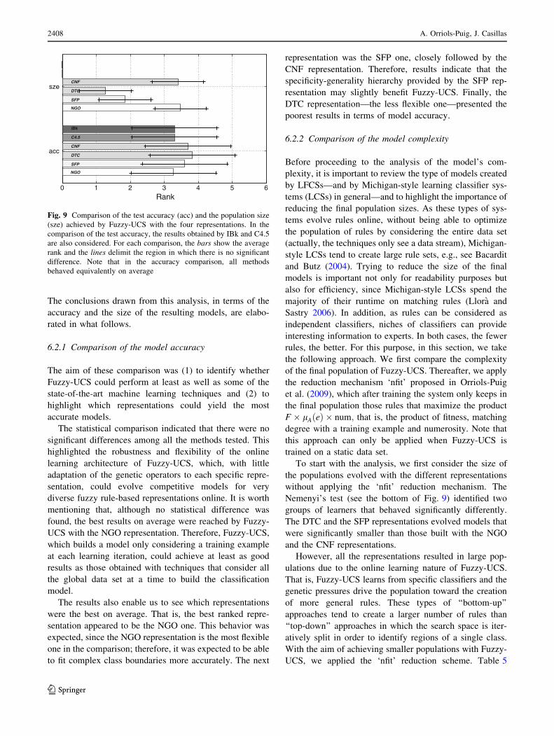
The conclusions drawn from this analysis, in terms of the
accuracy and the size of the resulting models, are elabo-
rated in what follows.
6.2.1 Comparison of the model accuracy
The aim of these comparison was (1) to identify whether
Fuzzy-UCS could perform at least as well as some of the
state-of-the-art machine learning techniques and (2) to
highlight which representations could yield the most
accurate models.
The statistical comparison indicated that there were no
significant differences among all the methods tested. This
highlighted the robustness and flexibility of the online
learning architecture of Fuzzy-UCS, which, with little
adaptation of the genetic operators to each specific repre-
sentation, could evolve competitive models for very
diverse fuzzy rule-based representations online. It is worth
mentioning that, although no statistical difference was
found, the best results on average were reached by Fuzzy-
UCS with the NGO representation. Therefore, Fuzzy-UCS,
which builds a model only considering a training example
at each learning iteration, could achieve at least as good
results as those obtained with techniques that consider all
the global data set at a time to build the classification
model.
The results also enable us to see which representations
were the best on average. That is, the best ranked repre-
sentation appeared to be the NGO one. This behavior was
expected, since the NGO representation is the most flexible
one in the comparison; therefore, it was expected to be able
to fit complex class boundaries more accurately. The next
representation was the SFP one, closely followed by the
CNF representation. Therefore, results indicate that the
specificity-generality hierarchy provided by the SFP rep-
resentation may slightly benefit Fuzzy-UCS. Finally, the
DTC representation—the less flexible one—presented the
poorest results in terms of model accuracy.
6.2.2 Comparison of the model complexity
Before proceeding to the analysis of the model’s com-
plexity, it is important to review the type of models created
by LFCSs—and by Michigan-style learning classifier sys-
tems (LCSs) in general—and to highlight the importance of
reducing the final population sizes. As these types of sys-
tems evolve rules online, without being able to optimize
the population of rules by considering the entire data set
(actually, the techniques only see a data stream), Michigan-
style LCSs tend to create large rule sets, e.g., see Bacardit
and Butz (2004). Trying to reduce the size of the final
models is important not only for readability purposes but
also for efficiency, since Michigan-style LCSs spend the
majority of their runtime on matching rules (Llora and
Sastry 2006). In addition, as rules can be considered as
independent classifiers, niches of classifiers can provide
interesting information to experts. In both cases, the fewer
rules, the better. For this purpose, in this section, we take
the following approach. We first compare the complexity
of the final population of Fuzzy-UCS. Thereafter, we apply
the reduction mechanism ‘nfit’ proposed in Orriols-Puig
et al. (2009), which after training the system only keeps in
the final population those rules that maximize the product
F � lAðeÞ � num; that is, the product of fitness, matching
degree with a training example and numerosity. Note that
this approach can only be applied when Fuzzy-UCS is
trained on a static data set.
To start with the analysis, we first consider the size of
the populations evolved with the different representations
without applying the ‘nfit’ reduction mechanism. The
Nemenyi’s test (see the bottom of Fig. 9) identified two
groups of learners that behaved significantly differently.
The DTC and the SFP representations evolved models that
were significantly smaller than those built with the NGO
and the CNF representations.
However, all the representations resulted in large pop-
ulations due to the online learning nature of Fuzzy-UCS.
That is, Fuzzy-UCS learns from specific classifiers and the
genetic pressures drive the population toward the creation
of more general rules. These types of ‘‘bottom-up’’
approaches tend to create a larger number of rules than
‘‘top-down’’ approaches in which the search space is iter-
atively split in order to identify regions of a single class.
With the aim of achieving smaller populations with Fuzzy-
UCS, we applied the ‘nfit’ reduction scheme. Table 5
0 1 2 3 4 5 6
acc
sze
NGO
SFP
DTC
CNF
C4.5
IBk
NGO
SFP
DTC
CNF
Rank
Fig. 9 Comparison of the test accuracy (acc) and the population size
(sze) achieved by Fuzzy-UCS with the four representations. In the
comparison of the test accuracy, the results obtained by IBk and C4.5
are also considered. For each comparison, the bars show the average
rank and the lines delimit the region in which there is no significant
difference. Note that in the accuracy comparison, all methods
behaved equivalently on average
2408 A. Orriols-Puig, J. Casillas
123
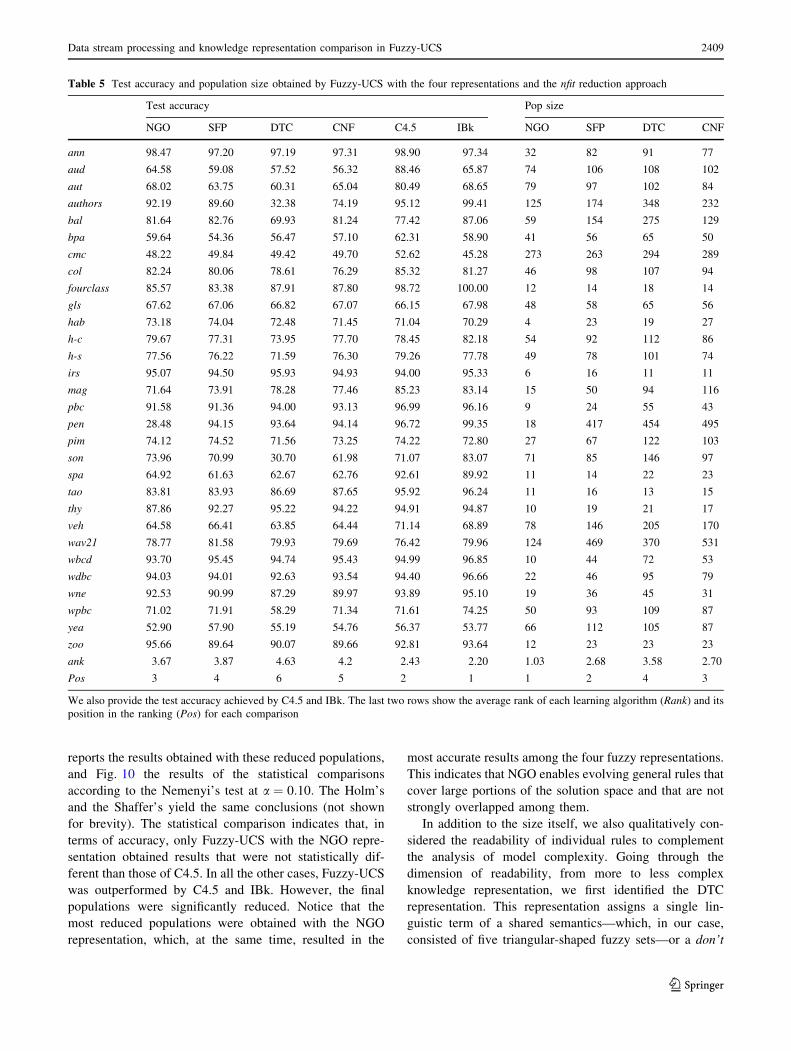
reports the results obtained with these reduced populations,
and Fig. 10 the results of the statistical comparisons
according to the Nemenyi’s test at a ¼ 0:10: The Holm’s
and the Shaffer’s yield the same conclusions (not shown
for brevity). The statistical comparison indicates that, in
terms of accuracy, only Fuzzy-UCS with the NGO repre-
sentation obtained results that were not statistically dif-
ferent than those of C4.5. In all the other cases, Fuzzy-UCS
was outperformed by C4.5 and IBk. However, the final
populations were significantly reduced. Notice that the
most reduced populations were obtained with the NGO
representation, which, at the same time, resulted in the
most accurate results among the four fuzzy representations.
This indicates that NGO enables evolving general rules that
cover large portions of the solution space and that are not
strongly overlapped among them.
In addition to the size itself, we also qualitatively con-
sidered the readability of individual rules to complement
the analysis of model complexity. Going through the
dimension of readability, from more to less complex
knowledge representation, we first identified the DTC
representation. This representation assigns a single lin-
guistic term of a shared semantics—which, in our case,
consisted of five triangular-shaped fuzzy sets—or a don’t
Table 5 Test accuracy and population size obtained by Fuzzy-UCS with the four representations and the nfit reduction approach
Test accuracy Pop size
NGO SFP DTC CNF C4.5 IBk NGO SFP DTC CNF
ann 98.47 97.20 97.19 97.31 98.90 97.34 32 82 91 77
aud 64.58 59.08 57.52 56.32 88.46 65.87 74 106 108 102
aut 68.02 63.75 60.31 65.04 80.49 68.65 79 97 102 84
authors 92.19 89.60 32.38 74.19 95.12 99.41 125 174 348 232
bal 81.64 82.76 69.93 81.24 77.42 87.06 59 154 275 129
bpa 59.64 54.36 56.47 57.10 62.31 58.90 41 56 65 50
cmc 48.22 49.84 49.42 49.70 52.62 45.28 273 263 294 289
col 82.24 80.06 78.61 76.29 85.32 81.27 46 98 107 94
fourclass 85.57 83.38 87.91 87.80 98.72 100.00 12 14 18 14
gls 67.62 67.06 66.82 67.07 66.15 67.98 48 58 65 56
hab 73.18 74.04 72.48 71.45 71.04 70.29 4 23 19 27
h-c 79.67 77.31 73.95 77.70 78.45 82.18 54 92 112 86
h-s 77.56 76.22 71.59 76.30 79.26 77.78 49 78 101 74
irs 95.07 94.50 95.93 94.93 94.00 95.33 6 16 11 11
mag 71.64 73.91 78.28 77.46 85.23 83.14 15 50 94 116
pbc 91.58 91.36 94.00 93.13 96.99 96.16 9 24 55 43
pen 28.48 94.15 93.64 94.14 96.72 99.35 18 417 454 495
pim 74.12 74.52 71.56 73.25 74.22 72.80 27 67 122 103
son 73.96 70.99 30.70 61.98 71.07 83.07 71 85 146 97
spa 64.92 61.63 62.67 62.76 92.61 89.92 11 14 22 23
tao 83.81 83.93 86.69 87.65 95.92 96.24 11 16 13 15
thy 87.86 92.27 95.22 94.22 94.91 94.87 10 19 21 17
veh 64.58 66.41 63.85 64.44 71.14 68.89 78 146 205 170
wav21 78.77 81.58 79.93 79.69 76.42 79.96 124 469 370 531
wbcd 93.70 95.45 94.74 95.43 94.99 96.85 10 44 72 53
wdbc 94.03 94.01 92.63 93.54 94.40 96.66 22 46 95 79
wne 92.53 90.99 87.29 89.97 93.89 95.10 19 36 45 31
wpbc 71.02 71.91 58.29 71.34 71.61 74.25 50 93 109 87
yea 52.90 57.90 55.19 54.76 56.37 53.77 66 112 105 87
zoo 95.66 89.64 90.07 89.66 92.81 93.64 12 23 23 23
ank 3.67 3.87 4.63 4.2 2.43 2.20 1.03 2.68 3.58 2.70
Pos 3 4 6 5 2 1 1 2 4 3
We also provide the test accuracy achieved by C4.5 and IBk. The last two rows show the average rank of each learning algorithm (Rank) and its
position in the ranking (Pos) for each comparison
Data stream processing and knowledge representation comparison in Fuzzy-UCS 2409
123

care symbol to each variable. Due to (1) the shared
semantics, (2) the low number of fuzzy partitions per
variable, and (3) the fact that each variable is assigned a
single linguistic term, this knowledge representation can be
easily read by human experts. With no doubt, if the ‘nfit’
reduction is not applied, DTC is the most appealing rep-
resentation in terms of complexity. On the other hand,
when ‘nfit’ is applied, DTC is the representation that allows
for a lower reduction of rules.
The CNF and the SFP representations come next in the
readability spectrum. The CNF representation differs from
the DTC one in the fact that it assigns a disjunction of lin-
guistic terms to each variable; the readability of the aggre-
gated fuzzy set, therefore, is more complex. On the other
hand, the SFP representation differs from the DTC one in the
fact that the shared semantics consists of a higher number of
linguistic terms with different widths (i.e., degrees of gen-
erality). Thus, although it is difficult to state in which of the
two representations the individual rules are more interpret-
able, both of them are far from the DTC representation.
Finally, the NGO representation is the less interpretable
one since variables do not share the same semantics any-
more, and so, human experts need to interpret each fuzzy
set separately. However, when applying the ‘nfit’ reduc-
tion, it results in the most reduced and most accurate rule
sets. Therefore, in this case, the NGO representation would
probably be the most appealing one.
The overall analysis conducted in this section has
illustrated that the online learning architecture of Fuzzy-
UCS can evolve very competitive models that use different
knowledge representations, emphasizing the flexibility of
the architecture. We have also shown an accuracy-inter-
pretability tradeoff that can be typically found in FRBCSs.
The results indicated that, if the user searches for the smallest
rule set possible, the best approach is to use the NGO rep-
resentation after applying the ‘nfit’ reduction mechanism.
On the other hand, if the user searches for maximum accu-
racy, the best approach is to use the NGO representation
without applying any type of reduction. In the middle of this
spectrum, we found the SFP representation, which resulted in
the second most accurate and most compact representation
regardless of whether the ‘nfit’ reduction was applied.
7 Learning each representation’s sweet spot
The study performed in the last section has highlighted
many important issues on the average behavior of each
particular representation. While the analysis of the com-
plexity denoted significant differences among the four
representations, the study of the performance could only
provide general comments based on the average behavior
of the four representations. However, looking at the
detailed results presented in Table 4, we can observe that
different representations excelled in distinct problems,
which may have diverse characteristics. Thus, the identi-
fication of which problem characteristics each representa-
tion is the best suited to appears as an appealing exercise.
The purpose of this section is to extend the analysis of the
accuracy of the four representations by characterizing the
complexity of the different problems and comparing the four
representations on the complexity space (Ho and Basu 2002),
with the aim of detecting the sweet spot where a particular
representation outperforms the others. With this idea in
mind, the next subsections first explain the analysis meth-
odology and then present the experimental conclusions.
7.1 Analysis methodology
To study the behavior of the different representations over
the complexity space, we first need to characterize the
problem complexity and then use this characterization in
our analysis. The following explains the method employed
to characterize different sources of problem difficulty.
Then, we use this characterization to define the problem of
automatically learning the characteristics that are the best
suited to each representation.
7.1.1 Problem complexity characterization
The characterization of the problem complexity was done
using the complexity measures designed by Ho and Basu
(2002). The authors defined a set of complexity measures
that extract different indicators of the class boundary
complexity. More specifically, the measures defined aimed
at measuring: (1) the overlaps in feature values from
0 1 2 3 4 5 6
acc
sze
NGO
SFP
DTC
CNF
C4.5
IBk
NGO
SFP
DTC
CNF
Rank
Fig. 10 Comparison of the test accuracy (acc) and the population
size (sze) achieved by Fuzzy-UCS with the four representations and
the nfit reduction. In the comparison of the test accuracy, the results
obtained by IBk and C4.5 are also considered. For each comparison,
the bars show the average rank and the lines delimit the region in
which there is no significant difference
2410 A. Orriols-Puig, J. Casillas
123

different classes, (2) the separability of classes, and (3) the
geometry, topology, and density of manifolds.
In our study, we selected the complexity measures
enumerated in Table 6, which are briefly explained as
follows. F1 is the Fisher’s discriminant ratio; high values of
F1 indicate that classes can be separated more easily. F2 is
the overlap of the per-class bounding boxes; high values of
this measure indicate that classes are highly overlapped,
and so, that it may be difficult to separate these classes. F3
is the maximum feature efficiency, which returns the pro-
portion of instances that a single attribute can discriminate;
thus, higher values denote that the instances of different
classes can be separated by a single attribute. F4 is the
collective feature efficiency4; it acts as F3, but it considers
the discriminative power of all the attributes of the problem.
N1 is the fraction of points on the class boundary, which
denotes the boundary length; high values of this measure are
usually associated to complex problems. N2 is the ratio of
average intra/inter-class nearest neighbor distance, which
compares the within-class spread with the distances to the
nearest neighbors of other classes; high values of N2 indicate
that the examples of the same class are disperse. N3 is the
leave-one-out error rate of the one-nearest neighbor classi-
fier; high values of N3 denote that classes are close in the
feature space. Finally, T1 is the fraction of maximum cov-
ering spheres; high values of this measure indicate that
instances are distributed in small clusters in the feature
space, and thus, that it may be difficult to fit the data accu-
rately. For more information about these measures, the
reader is referred to Ho and Basu (2002) and Ho et al. (2006).
7.1.2 Learning the sweet spot of each representation
We propose to transform the typical manual inspection of
results into a problem of automatically learning the domain
of excellence of each representation, i.e., the sweet spot on
the complexity space where a representation outperforms
the others.
For this purpose, let us define a classification problem
Pi: Each instance of the problem Pi corresponds to one of
the domains in the test bed (see Table 3), which is char-
acterized by the aforementioned complexity measures. The
label of each instance is the name of the representation that
obtained the best results (we consider the results of
Table 4). With this definition, we can use any machine
learning technique to model the domain of excellence of each
Fuzzy-UCS representation. This approach is related to the
work by Luengo and Herrera (2010), in which the authors
analyzed the behavior of a fuzzy system on the complexity
space, identifying regions of good and bad behavior of the
method. The main difference in our proposal is that we aim at
automatically identifying the sweet spot of each learner with
respect to the other methods included in the comparison.
We applied this procedure to the collection of 30 data
sets and used C4.5 (Quinlan 1993) to learn the domain of
excellence of the four representations included in the
comparison. We adopted C4.5 because of its tree repre-
sentation. The next subsection explains the results in detail.
7.2 Results
Figure 11 illustrates the decision tree learned by C4.5,
which explains the problem complexities to which each
representation is the best suited. Note that the tree does not
use the complexity measurements F3, N1 and N2, which
indicates that the remaining ones may suffice to identify the
sweet spot of each representation in this experiment and/or
that the complexity captured by these metrics is somehow
included in the remaining ones. The information provided
by the tree, which presented an accuracy of 86.66%, is
commented in the following.
The first attribute found in the tree traversal is F4, which
captures the collective capacity of problem features to
discriminate instances of different classes. Low values of
F4 are typically hard problems, while high values are easier
Table 6 Complexity measures used in our study
Id Measure High values
F1 Maximum Fisher’s discriminant ratio Classes can be discriminated more easily
F2 Overlap of the per-class bounding boxes Classes are highly overlapped
F3 Maximum (individual) feature efficiency An attribute can discriminate classes
F4 Collective feature efficiency All attributes together can discriminate classes
N1 Fraction of points on the class boundary Many points on the class boundary (complex boundary)
N2 Ratio of average intra/inter class nearest neighbor distance Examples of the same class are disperse
N3 Leave-one-out error rate of the one-nearest neighbor classifier Classes are close in the feature space
T1 Fraction of maximum covering spheres Instances distributed in small clusters of the same class
For each measure, we provide the identifier (Id), the measure name, and what high values of the measure means in terms of complexity
4 F4 is introduced here for the first time, and its design is based
on F3.
Data stream processing and knowledge representation comparison in Fuzzy-UCS 2411
123
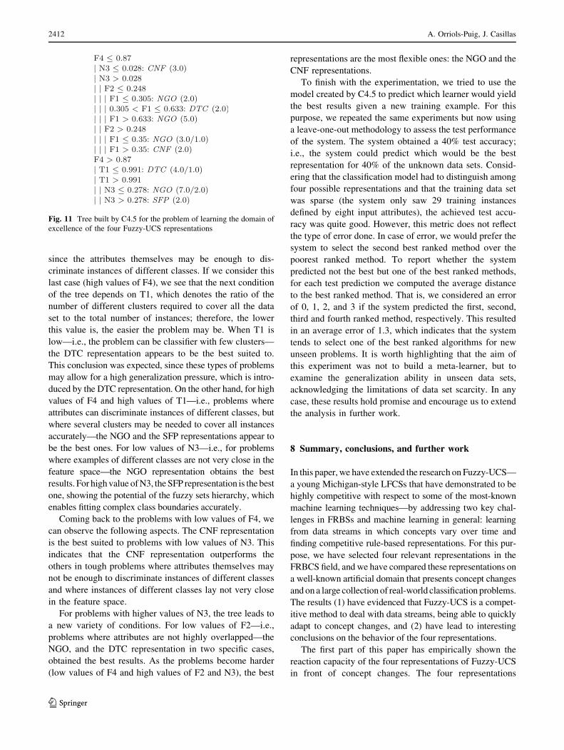
since the attributes themselves may be enough to dis-
criminate instances of different classes. If we consider this
last case (high values of F4), we see that the next condition
of the tree depends on T1, which denotes the ratio of the
number of different clusters required to cover all the data
set to the total number of instances; therefore, the lower
this value is, the easier the problem may be. When T1 is
low—i.e., the problem can be classifier with few clusters—
the DTC representation appears to be the best suited to.
This conclusion was expected, since these types of problems
may allow for a high generalization pressure, which is intro-
duced by the DTC representation. On the other hand, for high
values of F4 and high values of T1—i.e., problems where
attributes can discriminate instances of different classes, but
where several clusters may be needed to cover all instances
accurately—the NGO and the SFP representations appear to
be the best ones. For low values of N3—i.e., for problems
where examples of different classes are not very close in the
feature space—the NGO representation obtains the best
results. For high value of N3, the SFP representation is the best
one, showing the potential of the fuzzy sets hierarchy, which
enables fitting complex class boundaries accurately.
Coming back to the problems with low values of F4, we
can observe the following aspects. The CNF representation
is the best suited to problems with low values of N3. This
indicates that the CNF representation outperforms the
others in tough problems where attributes themselves may
not be enough to discriminate instances of different classes
and where instances of different classes lay not very close
in the feature space.
For problems with higher values of N3, the tree leads to
a new variety of conditions. For low values of F2—i.e.,
problems where attributes are not highly overlapped—the
NGO, and the DTC representation in two specific cases,
obtained the best results. As the problems become harder
(low values of F4 and high values of F2 and N3), the best
representations are the most flexible ones: the NGO and the
CNF representations.
To finish with the experimentation, we tried to use the
model created by C4.5 to predict which learner would yield
the best results given a new training example. For this
purpose, we repeated the same experiments but now using
a leave-one-out methodology to assess the test performance
of the system. The system obtained a 40% test accuracy;
i.e., the system could predict which would be the best
representation for 40% of the unknown data sets. Consid-
ering that the classification model had to distinguish among
four possible representations and that the training data set
was sparse (the system only saw 29 training instances
defined by eight input attributes), the achieved test accu-
racy was quite good. However, this metric does not reflect
the type of error done. In case of error, we would prefer the
system to select the second best ranked method over the
poorest ranked method. To report whether the system
predicted not the best but one of the best ranked methods,
for each test prediction we computed the average distance
to the best ranked method. That is, we considered an error
of 0, 1, 2, and 3 if the system predicted the first, second,
third and fourth ranked method, respectively. This resulted
in an average error of 1.3, which indicates that the system
tends to select one of the best ranked algorithms for new
unseen problems. It is worth highlighting that the aim of
this experiment was not to build a meta-learner, but to
examine the generalization ability in unseen data sets,
acknowledging the limitations of data set scarcity. In any
case, these results hold promise and encourage us to extend
the analysis in further work.
8 Summary, conclusions, and further work
In this paper, we have extended the research on Fuzzy-UCS—
a young Michigan-style LFCSs that have demonstrated to be
highly competitive with respect to some of the most-known
machine learning techniques—by addressing two key chal-
lenges in FRBSs and machine learning in general: learning
from data streams in which concepts vary over time and
finding competitive rule-based representations. For this pur-
pose, we have selected four relevant representations in the
FRBCS field, and we have compared these representations on
a well-known artificial domain that presents concept changes
and on a large collection of real-world classification problems.
The results (1) have evidenced that Fuzzy-UCS is a compet-
itive method to deal with data streams, being able to quickly
adapt to concept changes, and (2) have lead to interesting
conclusions on the behavior of the four representations.
The first part of this paper has empirically shown the
reaction capacity of the four representations of Fuzzy-UCS
in front of concept changes. The four representations
Fig. 11 Tree built by C4.5 for the problem of learning the domain of
excellence of the four Fuzzy-UCS representations
2412 A. Orriols-Puig, J. Casillas
123
appeared to be more robust than IBk with a global window
equal to the number of examples sampled per concept, a
system that is usually employed to set a baseline in these
types of analyses. Besides, Fuzzy-UCS with the NGO
representation reported results that were significantly better
than those obtained by one of the most competitive data
stream miners, OnlineTree2, in the SEA problem. We have
also shown that the NGO and CNF representations adapt
well the concept changes even when the number of input
variables that define the concept increase.
Thereafter, the comparison has been extended to a large
collection of real-world problems. We have moved on to
domains in which concepts do not change over time due to
the lack of real-world classification problems with concept
drift. This experimental analysis has yielded two important
conclusions. The first conclusion was that the four repre-
sentations resulted in models whose accuracy (1) was not
significantly different among them and (2) was not sig-
nificantly different from that of the models created by IBk
and C4.5, two of the most-influential machine learning
techniques to process data sets with static concepts. On the
other hand, there were significant differences among the
complexity of the models obtained with the four different
representations of Fuzzy-UCS. The second conclusion was
that, taking the average behavior in account, we could
observe that the most flexible—and so, less readable—
representations resulted in the most accurate results,
drawing an accuracy-interpretability tradeoff that can be
usually found in FRBCS.
Although the typical approach in machine learning
comparisons is to extract conclusions on the average
behavior of learners, here we were also interested in
empowering this analysis by examining which types of
problem characteristics benefited the different representa-
tions. For this purpose, we proposed to move the com-
parison to the complexity space to identify the sweet spot
in which each particular representation excelled. We
employed a set of complexity measures to characterize
different sources of difficulty and fed these indicators as
input values of the problem of learning the domain of
excellence of each representation. This exercise generated
interesting results which explained the different charac-
teristics that were beneficial/detrimental to the different
representations. It was interesting to note that most of these
explanations followed the initial intuition of when a rep-
resentation should be better than the others. In addition, the
prediction capacity of the models built by C4.5 was tested,
resulting in a quite good behavior despite the high scarcity
of the training data set employed.
The analysis on the complexity space opens up future
work lines. In particular, we are interested in extending the
analysis on the complexity space by including a higher
number of real-world problems and the design of new
complexity measures that enable us to capture new sources
of problem complexity. This would serve to create even
more accurate domains of excellence, which could be used
to design meta-classifier mechanisms that decide which
knowledge representation should be evolved depending on
the intrinsic complexities of the each particular problem.
Acknowledgments The authors would like to warmly thank Marlon
Nunez, Raul Fidalgo, and Rafael Morales from the Universidad deMalaga for providing us with the experimental results of Online-
Tree2. The authors thank the support of Ministerio de Ciencia yTecnologıa under projects TIN2008-06681-C06-01 and TIN2008-
06681-C06-05, Generalitat de Catalunya under Grant 2005SGR-
00302, and Andalusian Government under grant P07-TIC-3185.
References
Abbass HA, Bacardit J, Butz MV, Llora X (2004) Online adaptation
in learning classifier systems: stream data mining. IlliGAL report
2004031. Illinois Genetic Algorithms Laboratory, University of
Illinois at Urbana-Champaign
Aggarwal C (ed) (2007) Data streams: models and algorithms.
Springer, Berlin
Aha D, Kibler D, Albert M (1991) Instance-based learning algo-
rithms. Mach Learn 6(1):37–66
Alcala R, Casillas J, Cordon O, Herrera F (2001) Building fuzzy
graphs: features and taxonomy of learning for non-grid-oriented
fuzzy rule-based systems. J Intell Fuzzy Syst 11(3–4):99–119
Angelov P, Lughofer E, Zhou X (2008) Evolving fuzzy classifiers
using different model architectures. Fuzzy Sets Syst 159(23):
3160–3182
Asuncion A, Newman DJ (2007) UCI Machine Learning Reposi-
tory. University of California. http://www.ics.uci.edu/*mlearn/
MLRepository.html
Bacardit J, Butz MV (2004) Data mining in learning classifier
systems: comparing XCS with GAssist. In: Proceedings of the
7th international workshop on learning classifier systems.
Springer
Botta A, Lazzerini B, Marcelloni F, Stefanescu DC (2009) Context
adaptation of fuzzy systems through a multi-objective evolu-
tionary approach based on a novel interpretability index. Soft
Comput 13(5):437–449
Butz MV, Sastry K, Goldberg DE (2005) Strong, stable, and reliable
fitness pressure in XCS due to tournament selection. Genet
Program Evolvable Mach 6(1):53–77
Carse B, Fogarty TC, Munro A (1996) Evolving fuzzy rule based
controllers using genetic algorithms. Fuzzy Sets Syst 80:273–294
Casillas J, Cordon O, del Jesus MJ, Herrera F (2005) Genetic tuning
of fuzzy rule deep structures preserving interpretability and its
interaction with fuzzy rule set reduction. IEEE Trans Fuzzy Syst
13(1):13–29
Choi JN, Oh SK, Pedrycz W (2008) Identification of fuzzy models
using a successive tuning method with a variant identification
ratio. Fuzzy Sets Syst 159(21):2873–2889
Cooper MG, Vidal JJ (1994) Genetic design of fuzzy controllers: the
cart and jointed pole problem. In: Proceedings of the 3rd IEEE
international conference on fuzzy systems, Piscataway, NJ,
USA, pp 1332–1337
Cordon O, Herrera F (1997) A three-stage evolutionary process for
learning descriptive and approximate fuzzy logic controller
knowledge bases from examples. Int J Approx Reason 17(4):
369–407
Data stream processing and knowledge representation comparison in Fuzzy-UCS 2413
123

Cordon O, del Jesus MJ, Herrera F (1999) A proposal on reasoning
methods in fuzzy rule-based classification systems. Int J Approx
Reason 20(1):21–45
del Campo-Avila J, Ramos-Jimenez G, Gama J, Morales-Bueno R
(2008) Improving the performance of an incremental algorithm
driven by error margins. Intell Data Anal 12(3):305–318
Demsar J (2006) Statistical comparisons of classifiers over multiple
data sets. J Mach Learn Res 7:1–30
Dietterich TG (1998) Approximate statistical tests for comparing
supervised classification learning algorithms. Neural Comput
10(7):1895–1924
Domingos P, Hulten G (2000) Mining high-speed data streams. In:
KDD’00: Proceedings of the sixth ACM SIGKDD international
conference on knowledge discovery and data mining. ACM,
New York, NY, USA, pp 71–80
Fernandez A, del Jesus M, Herrera F (2009) Hierarchical fuzzy rule
based classification systems with genetic rule selection for
imbalanced data-sets. Int J Approx Reason 50(3):561–577
Friedman M (1937) The use of ranks to avoid the assumption of
normality implicit in the analysis of variance. J Am Stat Assoc
32:675–701
Friedman M (1940) A comparison of alternative tests of significance
for the problem of m rankings. Ann Math Stat 11:86–92
Fritzke B (1997) Incremental neuro-fuzzy systems. In: Proceedings of
the international society for optical engineering: applications of
soft computing, vol 3165, pp 86–97
Gacto M, Alcala R, Herrera F (2009) Adaptation and application of
multi-objective evolutionary algorithms for rule reduction and
parameter tuning of fuzzy rule-based systems. Soft Comput
13(5):419–436
Gama J, Gaber MM (eds) (2007) Learning from data streams.
Springer, Heidelberg
Gama J, Rocha R, Medas P (2003) Accurate decision trees for mining
high-speed data streams. In: KDD ’03: Proceedings of the ninth
ACM SIGKDD international conference on knowledge discov-
ery and data mining, ACM, New York, NY, USA, pp 523–528
Gama J, Medas P, Castillo G, Rodrigues P (2004) Learning with drift
detection. In: Proceedings of the 17th Brasilian symposium on
artificial intelligence, pp 286–295
Garcıa S, Herrera F (2008) An extension on ‘‘statistical comparisons
of classifiers over multiple data sets’’ for all pairwise compar-
isons. J Mach Learn Res 9:2677–2694
Goldberg DE (1989) Genetic algorithms in search, optimization &
machine learning, 1st edn. Addison Wesley, Reading, MA
Goldberg DE (2002) The design of innovation: lessons from and for
competent genetic algorithms, 1st edn. Kluwer Academic
Publishers, Boston, MA
Gonzalez A, Perez R (1998) Completeness and consistency condi-
tions for learning fuzzy rules. Fuzzy Sets Syst 96(1):37–51
Ho TK, Basu M (2002) Complexity measures of supervised
classification problems. IEEE Trans Pattern Anal Mach Intell
24(3):289–300
Ho TK, Basu M, Law M (2006) Measures of geometrical complexity
in classification problems. In: Basu M, Ho TK (eds) Data
complexity in pattern recognition. Springer, London, pp 1–23
Holland JH (1975) Adaptation in natural and artificial systems. The
University of Michigan Press, Ann Arbor, MI
Ishibuchi H, Nakashima T (2001) Effect of rule weights in fuzzy rule-
based classification systems. IEEE Trans Fuzzy Syst 9(4):506–
515
Ishibuchi H, Nojima Y (2007) Analysis of interpretability-accuracy
tradeoff of fuzzy systems by multiobjective fuzzy genetics-based
machine learning. Int J Approx Reason 44(1):4–31
Ishibuchi H, Yamamoto T (2005) Rule weight specification in fuzzy
rule-based classification systems. IEEE Trans Fuzzy Syst 13(4):
428–435
Ishibuchi H, Nozaki K, Tanaka H (1992) Distributed representation of
fuzzy rules and its application to pattern classification. Fuzzy
Sets Syst 52(1):21–32
Ishibuchi H, Murata T, Turksen IB (1997) Single-objective and two-
objective genetic algorithms for selecting linguistic rules for
pattern classification problems. Fuzzy Sets Syst 89(2):135–150
Ishibuchi H, Nakashima T, Murata T (1999) Performance evaluation
of fuzzy classifier systems for multidimensional pattern classi-
fication problems. IEEE Trans Syst Man Cybern Part B Cybern
29(5):601–618
Ishibuchi H, Yamamoto T, Nakashima T (2005) Hybridization of
fuzzy GBML approaches for pattern classification problems.
IEEE Trans Syst Man Cybern Part B Cybern 35(2):359–365
Ishibuchi H, Kaisho Y, Nojima Y (2009) Complexity, interpretability
and explanation capability of fuzzy rule-based classifiers. In:
Proceedings of the IEEE international conference on fuzzy
systems, Jeju, Korea, pp 1730–1735
Jong KAD, Spears WM, Gordon D (1993) Using genetic algorithms
for concept learning. Genet algorithms Mach Learn (Special
Issue of Machine Learning) 13(2–3):161–188
Llora X, Sastry K (2006) Fast rule matching for learning classifier
systems via vector instructions. In: GECCO ’06: Proceedings of
the 8th annual conference on genetic and evolutionary compu-
tation. ACM, New York, NY, USA, pp 1513–1520
Luengo J, Herrera F (2010) Domains of competence of fuzzy rule
based classification systems with data complexity measures: a
case of study using a fuzzy hybrid genetic based machine
learning method. Fuzzy Sets Syst 161(1):3–19
Maloof MA, Michalski RS (2004) Incremental learning with partial
instance memory. Artif Intell 154(1–2):95–126
Michalski R (1983) A theory and methodology of inductive learning.
Artif Intell 20:111–161
Nemenyi PB (1963) Distribution-free multiple comparisons. PhD
thesis. Princeton University, New Jersey, USA
Nunez M, Fidalgo R, Morales R (2007) Learning in environments
with unknown dynamics: towards more robust concept learners.
J Mach Learn Res 8:2595–2628
Orriols-Puig A, Casillas J, Bernado-Mansilla E (2008) Evolving fuzzy
rules with UCS. In: Advances at the frontier of LCSs. Springer,
LNCS, vol 4998, pp 57–76
Orriols-Puig A, Casillas J, Bernado-Mansilla E (2009) Fuzzy-UCS: a
Michigan-style learning fuzzy-classifier system for supervised
learning. IEEE Trans Evolut Comput 13(2):1093–1119
Pulkkinen P, Koivisto H (2010) A dynamically constrained multiob-
jective genetic fuzzy system for regression problems. IEEE
Trans Fuzzy Syst 18(1):161–177
Quinlan JR (1993) C4.5: Programs for machine learning. Morgan
Kaufmann Publishers, San Mateo, CA
Sheskin D (2000) Handbook of parametric and nonparametric
statistical procedures. Chapman & Hall, Boca Raton
Street WN, Kim Y (2001) A streaming ensemble algorithm (sea) for
large-scale classification. In: KDD ’01: Proceedings of the
seventh ACM SIGKDD international conference on knowledge
discovery and data mining. ACM, New York, NY, USA,
pp 377–382
Widmer G, Kubat M (1996) Learning in the presence of concept drift
and hidden contexts. Mach Learn 23(1):69–101
Wilson SW (1998) Generalization in the XCS classifier system. In:
Proceedings of the 3rd annual conference on genetic program-
ming, Morgan Kaufmann, pp 665–674
Witten I, Frank E (2005) Data mining: practical machine learning
tools and techniques, 2nd edn. Morgan Kaufmann, San Francisco
Wu X, Kumar V, Quinlan JR, Ghosh J, Yang Q, Motoda H,
McLachlan GJ, Ng A, Liu B, Yu PS, Zhou ZH, Steinbach M,
Hand DJ, Steinberg D (2007) Top 10 algorithms in data mining.
Knowl Inform Syst 14(1):1–37
2414 A. Orriols-Puig, J. Casillas
123


![Fuzzy Mortality Model Based on Banach Algebra · Fuzzy Mortality Model Based on Banach Algebra 247 Property 1 Representation theorem for arbitrary fuzzy number [4]. An arbitrary fuzzy](https://img.pdfslide.net/doc/110x75/5bade01f09d3f290738bca3b/fuzzy-mortality-model-based-on-banach-fuzzy-mortality-model-based-on-banach.jpg)


![Small-Task Incremental LearningSmall-Task Incremental Learning 3 Hou et al. [12], in the method called here UCIR, made representation learning explicit, by noticing that the limited](https://img.pdfslide.net/doc/110x75/5f0b478d7e708231d42fbb6b/small-task-incremental-learning-small-task-incremental-learning-3-hou-et-al-12.jpg)