Embed Size (px)
Citation preview

FUZZY SLIDING MODE CONTROL FOR CART
INVERTED PENDULUM SYSTEM
BELAL AHMED ABDELAZIZ ELSAYED
FACULTY OF ENGINEERING
UNIVERSITY OF MALAYA
KUALA LUMPUR
2013

FUZZY SLIDING MODE CONTROL FOR CART
INVERTED PENDULUM SYSTEM
BELAL AHMED ABDELAZIZ ELSAYED
THESIS SUBMITTED IN FULFILLMENT OF THE
REQUIREMENTS FOR THE DEGREE OF MASTER OF
ENGINEERING SCIENCE
FACULTY OF ENGINEERING
UNIVERSITY OF MALAYA
KUALA LUMPUR
2013

iii
Abstract
Cart Inverted Pendulum (CIP) is a benchmark problem in nonlinear automatic control
which has numerous applications, such as two wheeled mobile robot and under actuated
robots. The objective of this study is to design a swinging-up controller with a robust
sliding mode stabilization controller for CIP, and to apply the proposed controller on a real
CIP. Two third-order differential equations were derived to create a combining model for
the cart-pendulum with its DC motor dynamics, where the motor voltage is considered as
the system input. The friction force between the cart and rail was included in the system
equations through a nonlinear friction model. A Fuzzy Swinging-up controller was
designed to swing the pendulum toward the upright position, with consideration of the cart
rail limits. Once the pendulum reaches the upward position, Sliding Mode Controller
(SMC) is activated, to balance the system. For comparison purposes, a Linear Quadratic
Regulator Controller (LQRC) was design and compared with proposed SMC. Simulation
and experimental results have shown a significant improvement of the proposed SMC over
LQRC where, the pendulum angle oscillations were decreased by 80% in the real
implementation.

iv
Abstrak
Troli bandul Inverted (CIP) sistem adalah masalah penanda aras dalam kawalan automatik
linear. Terdapat banyak aplikasi untuk CIP dalam kehidupan kita, seperti dua robot beroda
mudah alih yang dianggap sebagai pengangkutan era peribadi baru. Tujuan kajian ini ialah
untuk merekabentuk pengawal berayun-up dengan pengawal penstabilan mantap untuk
CIPS dan memohon pengawal kepada sistem sebenar. Dalam mod sistem, dua persamaan
pembezaan tertib ketiga diperoleh untuk mewujudkan satu model yang menggabungkan
untuk bandul cart dengan motor dinamik DC. Dalam model yang dibentangkan voltan
motor dianggap sebagai input sistem dan semua batasan praktikal dianggap. Daya geseran
antara cart dan rel telah dimasukkan ke dalam sistem persamaan melalui model geseran tak
linear. A Fuzzy berayun-up pengawal telah direka untuk ayunan bandul untuk kedudukan
tegak dalam pertimbangan had rel cart. Setelah bandul mencapai kedudukan menaik,
Ketiga-perintah gelongsor Mod Pengawal (SMC) diaktifkan, untuk mengimbangi sistem.
Dalam usaha untuk mengesahkan prestasi SMC dicadangkan Pengawal Pengawal Selia
Linear kuadratik (LQRC) telah dicadangkan dan berbanding dengan cadangan SMC.
Simulasi dan eksperimen keputusan telah menunjukkan peningkatan yang ketara SMC
dicadangkan lebih LQRC mana, sudut ayunan bandul telah menurun sebanyak 80% dalam
pelaksanaan sebenar.

v
Acknowledgment
“Allah taught you that which you knew not. And Ever Great is the Grace of
Allah unto you” (Surat Al-Nisa verse 113)
First, I want to thank ALLAH for his Grace and for giving me the strength to finish this
work. Thanks for my supervisors Prof. Saad Mekhelif and Ass.Prof. Mohsen Abdelnaiem
for their patience, guidance and encouragement during all my studying stages. I am also
grateful for their confidence and freedom they gave during this work.
Special thanks go to my big family, my parent and my siblings, for their kind help and
understanding. Also I want to express my gratitude to Aalaa, my wife, for her continues
support during two years of a hard work.
Finally, I would like to thank all my colleagues in the University of Malaya for this great
time of exchanging knowledge and experiences.
vi
Table of Contents
Abstract ................................................................................................................................. iii
Abstrak .................................................................................................................................. iv
Acknowledgment .................................................................................................................... v
Table of Contents .................................................................................................................. vi
List of Figures ....................................................................................................................... ix
List of Tables ........................................................................................................................ xi
List of Abbreviation ............................................................................................................. xii
List of Symbols ................................................................................................................... xiii
Chapter one ............................................................................................................................. 1
1 Introduction...................................................................................................................... 1
1.1 Introduction ............................................................................................................. 1
1.2 Inverted Pendulum System ...................................................................................... 1
1.3 Fuzzy Logic Control ................................................................................................ 5
1.4 Sliding Mode Control .............................................................................................. 6
1.5 Objectives ................................................................................................................ 7
1.6 Thesis outline .......................................................................................................... 8
Chapter Two .......................................................................................................................... 10
2 Literature Review .......................................................................................................... 10
2.1 Introduction ........................................................................................................... 10
2.2 Swinging-up controllers ........................................................................................ 11
2.3 Stabilization controllers ......................................................................................... 13
2.3.1 Linear Stabilization controllers ...................................................................... 13
2.3.2 Nonlinear Stabilization controllers ................................................................ 14

vii
2.4 Study plan .............................................................................................................. 16
Chapter Three ........................................................................................................................ 17
3 Mathematical model ...................................................................................................... 17
3.1 Introduction ........................................................................................................... 17
3.2 Pendulum model .................................................................................................... 17
3.3 Friction model ....................................................................................................... 21
3.4 Dc Motor model .................................................................................................... 22
3.5 Overall system model ............................................................................................ 23
Chapter Four ......................................................................................................................... 30
4 Methodology .................................................................................................................. 30
4.1 Introduction ........................................................................................................... 30
4.2 Fuzzy swing-up controller ..................................................................................... 30
4.3 Sliding Mode stabilization controller .................................................................... 37
4.4 LQR stabilization controller .................................................................................. 42
4.5 Switching between swinging-up and stabilization control .................................... 45
Chapter Five .......................................................................................................................... 46
5 Simulation results .......................................................................................................... 46
5.1 Introduction ........................................................................................................... 46
5.2 Fuzzy swinging-up with SMC stabilization .......................................................... 47
5.3 Fuzzy swinging up with LQR stabilization controller .......................................... 49
Chapter Six ............................................................................................................................ 52
6 Experimental results ...................................................................................................... 52
6.1 Introduction ........................................................................................................... 52
6.2 Experimental setup ................................................................................................ 52
6.2.1 Electro- mechanical setup .............................................................................. 52
6.2.2 Real time controller setup .............................................................................. 54
6.2.3 Velocity and acceleration estimation ............................................................. 55
6.3 Fuzzy swinging with SMC experimental results ................................................... 56

viii
6.4 Fuzzy swinging with LQR experimental results ................................................... 58
Chapter Seven ....................................................................................................................... 61
7 Comparison results and discussion ................................................................................ 61
7.1 Introduction ........................................................................................................... 61
7.2 Simulation comparison .......................................................................................... 61
7.3 Experimental comparison ...................................................................................... 63
Chapter Eight ........................................................................................................................ 65
8 Conclusion and Future work .......................................................................................... 65
8.1 Conclusion ............................................................................................................. 65
8.2 Future work ........................................................................................................... 66
References ............................................................................................................................. 67
Appendix 1 ............................................................................................................................ 74
Appendix 2 ............................................................................................................................ 76
Appendix 3 ............................................................................................................................ 77
Appendix 4 ............................................................................................................................ 79

ix
List of Figures
Figure 1.1: Inverted pendulum swinging-up .......................................................................... 2
Figure 1.2: Segway robot(Segway, 2012) .............................................................................. 2
Figure 1.3: Flying under actuated robots (Tedrake, 2009). ................................................... 3
Figure 1.4: Rat under actuated robot (Tedrake, 2009). .......................................................... 4
Figure 1.5: Cart Inverted Pendulum ....................................................................................... 4
Figure 1.6: Furuta Pendulum (Buckingham, 2003). .............................................................. 5
Figure 1.7: Fuzzy control process. ......................................................................................... 6
Figure 3.1: The Cart-Pendulum system ............................................................................... 17
Figure 3.2: Cart free body diagram ...................................................................................... 18
Figure 3.3: Pendulum free body diagram............................................................................. 19
Figure 3.4: DC Motor circuit ............................................................................................... 22
Figure4.1: schematic diagram for Swing up with stabilization controller. .......................... 30
Figure 4.2: Membership functions of the pendulum angle. ................................................. 31
Figure 4.3: Membership functions of the pendulum angular velocity. ................................ 32
Figure 4.4: Membership functions of the cart position. ...................................................... 33
Figure 4.5 : Membership functions of the output control voltage. ...................................... 33
Figure 5.1: Pendulum angular position response for fuzzy swing-up with SMC. ............... 48
Figure 5.2: Cart position response for fuzzy swing-up with SMC. ..................................... 48
Figure 5.3: Control voltage response for fuzzy swing-up with SMC. ................................. 49
Figure 5.4: Pendulum angular position response for fuzzy swing-up with LQRC. ............. 50
Figure 5.5: Cart position response for fuzzy swing-up with LQRC. ................................... 51
Figure5.6 : Control voltage response for fuzzy swing-up with LQRC. ............................... 51

x
Figure 6.1: CIP model IP02 ................................................................................................. 53
Figure 6.2: CIP cart with DC motor. .................................................................................... 53
Figure 6.3: AD/DA card terminal board .............................................................................. 54
Figure 6.4: Power module. ................................................................................................... 55
Figure 6.5: Schematic diagram for the fitting process. ........................................................ 56
Figure 6.6: Experimental result for pendulum angular position with Fuzzy swing up and
SMC. .................................................................................................................................... 57
Figure 6.7:. Experimental result for cart position for Fuzzy swing up with SMC.............. 57
Figure 6.8: Experimental result for control voltage for Fuzzy swing up with SMC. .......... 58
Figure 6.9: Experimental result for pendulum angular position with Fuzzy swing up with
LQRC. .................................................................................................................................. 59
Figure 6.10: Experimental result for cart position with Fuzzy swing up with LQRC. ....... 59
Figure 6.11: Experimental result for control voltage for Fuzzy swing up with LQRC. ..... 60
Figure 7.1 : Pendulum angular position response under disturbance. ................................. 62
Figure 7.2: Cart position response under disturbance. ......................................................... 62
Figure 7.3: Pendulum angle experimental result. ................................................................ 63
Figure 7.4: Cart position experimental result....................................................................... 64
Figure 7.5:. Control voltage experimental result. ............................................................... 64

xi
List of Tables
Table 5.1: System parameters………………..……………………………47

xii
List of Abbreviation
IP: Inverted Pendulum
CIP: Cart-Inverted Pendulum
SMC: Sliding Mode Controller
CW: Clock Wise
CCW: Counter Clock Wise
FLC: Fuzzy Logic Control
KBFC: Knowledge Based Fuzzy Control
FBL: Feedback Linearization.
PID: Proportional–integral–derivative
CG: Center of Gravity
LQRC: Linear Quadratic Regulator Controller
DC: Direct Current
EMF: Elector Magnetic Force
PC: Personal Computer
AD/DA: Analog to Digital/Digital to Analog
SISO: Single-Input Single-Output
SIMO: Single-Input Multi-Output

xiii
List of Symbols
X Cart displacement
Pendulum angle
X Cart velocity
Pendulum Angular velocity
X Cart acceleration
Pendulum angular acceleration
aV DC motor applied voltage
i DC motor armature current
aL DC motor armature Inductance
aR DC motor armature resistance
DC Motor angular velocity
eT DC Motor torque
jT DC Motor inertia torque
BT DC Motor damping torque
LT DC Motor load torque
M Cart Mass
m Pendulum mass
L Pendulum length (From the pivot to the center of gravity)
F Applied force on the cart
frF Friction force between the cart and the rail
q Friction coefficient between the pendulum and the pivot
I Pendulum mass moment of inertia around the C.G

xiv
J DC motor rotor mass moment of inertia
tK Motor Torque constant
eK Back EMF constant
r DC Motor pulley Diameter
B Motor rotor damping coefficient
FS Static Friction force
FC Coulumb Friction force
Xd Dead zone velocities
VS Stribeck velocity
n Friction form factor
b Viscous friction coefficient.

1
Chapter one
1 Introduction
1.1 Introduction
Controlling of nonlinear systems could be classified into two main categories. In the first
one, the system is approximated into linear model, where the classical control theories are
applied directly. This method of analysis is much simpler since it avoids dealing with the
complicated mathematics due to systems nonlinearity. The global stability cannot be
achieved because of neglecting the nonlinear effects.
On the other hand, nonlinear control techniques are applied to guarantee the global
stability and to improve the system response. Advanced mathematical tools are
necessitated to analyze the exact nonlinear models, and for stability guarantee (Khalil,
2002).
1.2 Inverted Pendulum System
Inverted Pendulum (IP) is an essential bench mark problem in nonlinear control. It is a
challenging problem for control engineers because of system nonlinearity and instability. IP
is a normal pendulum in the upright position which could be controlled by moving the pivot
point in the horizontal plan. Swinging up and stabilization of IP is a fundamental problem
in control field. In this task, the pendulum is swung from the downward (stable) position to

2
the upward (unstable) position. Then, the stabilization controller is applied to keep the
pendulum stable in that position, as it is shown in Figure 1.1 (Rubi et al., 2002).
Figure 1.1: Inverted pendulum swinging-up
In the real life, there are many applications for IP, for example, two wheeled mobile robot
which is known commercially as Segway robot, Figure 1.2. This robot model is similar to
IP where, the pendulum and the pivot are replaced with the robot body and the two-wheels,
respectively. The wheels are power-driven by an electric motor to keep the robot stable
(Cardozo andVera, 2012) .
Figure 1.2: Segway robot(Segway, 2012)
3
Nowadays, Segway has been utilized in airports, malls, ect, by the security guards and
workers, in order to save their time and efforts. It is expected to be the new era personal
transports during the next decades (Voth, 2005) . Rockets and missiles are considered as IP
applications, where the system is unstable during the initial stage of flight. Controlling of
IP might be used to be applied in rockets to control the throttle angle.
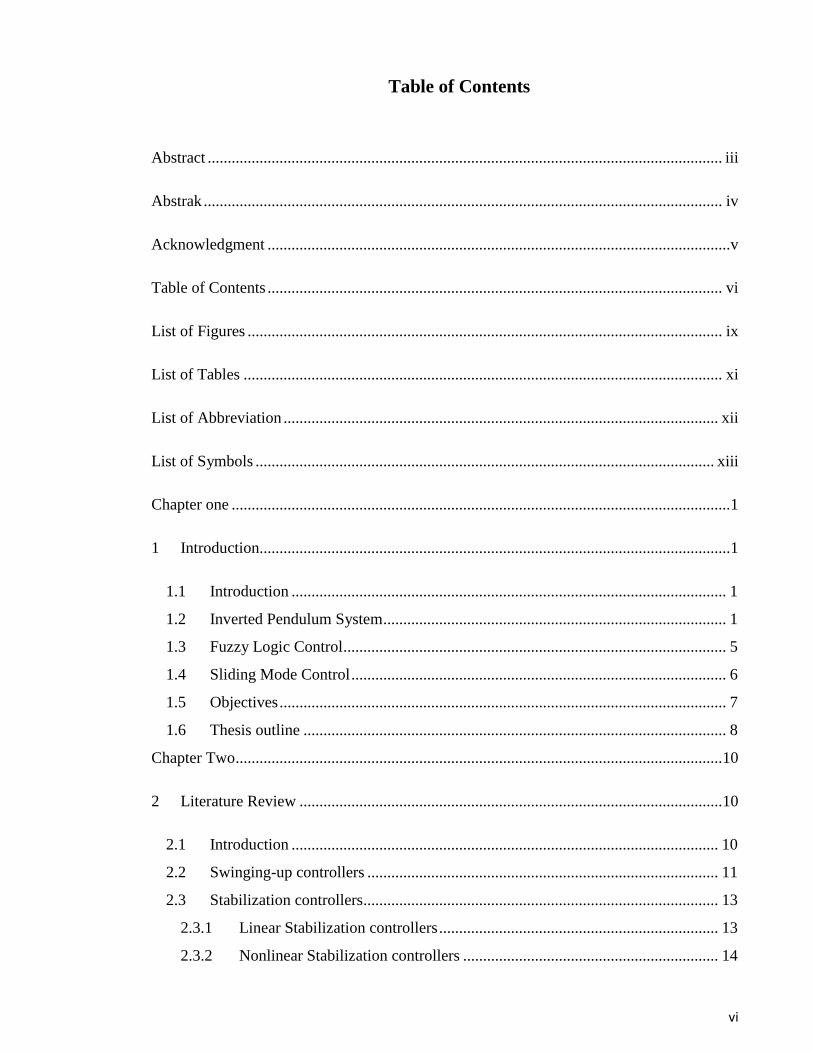
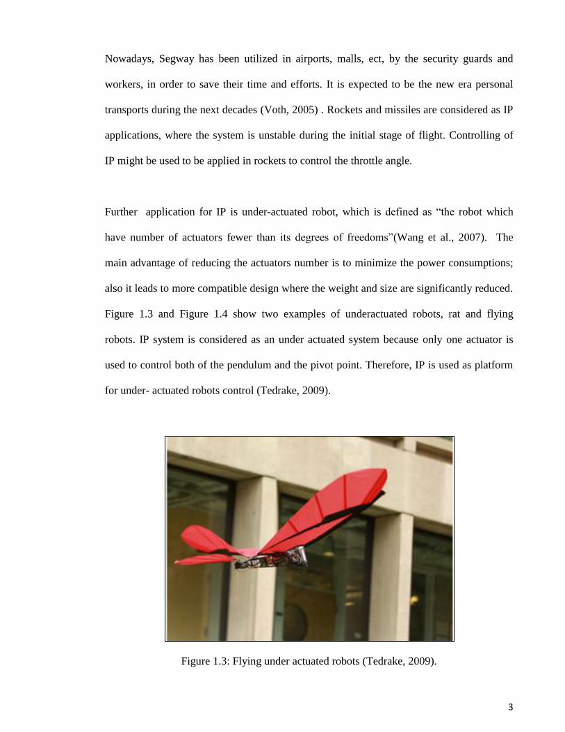
Further application for IP is under-actuated robot, which is defined as “the robot which
have number of actuators fewer than its degrees of freedoms”(Wang et al., 2007). The
main advantage of reducing the actuators number is to minimize the power consumptions;
also it leads to more compatible design where the weight and size are significantly reduced.
Figure 1.3 and Figure 1.4 show two examples of underactuated robots, rat and flying
robots. IP system is considered as an under actuated system because only one actuator is
used to control both of the pendulum and the pivot point. Therefore, IP is used as platform
for under- actuated robots control (Tedrake, 2009).
Figure 1.3: Flying under actuated robots (Tedrake, 2009).
4
Figure 1.4: Rat under actuated robot (Tedrake, 2009).
In control laboratories, two types of IP could be found, based on the pivot point motion,
linear or angular. In linear type, the pivot point is fixed to a cart which moves on
horizontally on a rail, the cart is driven by an electrical motor (usually DC motor). This
type is well known as Cart-Inverted Pendulum (CIP), Figure 1.5 (Das andPaul, 2011) . In
the angular type, the pivot motion is angular and it is also driven by an electric motor. It is
sometimes known as Futura Pendulum (Japanese scientist), see Figure 1.6 (Shiriaev et al.,
2007). Swinging-up of CIP is more challengeable because of the cart rail limits, in contrast
to Furuta pendulum where the pivot motion is boundless.
Figure 1.5: Cart Inverted Pendulum

5
Figure 1.6: Furuta Pendulum (Buckingham, 2003).
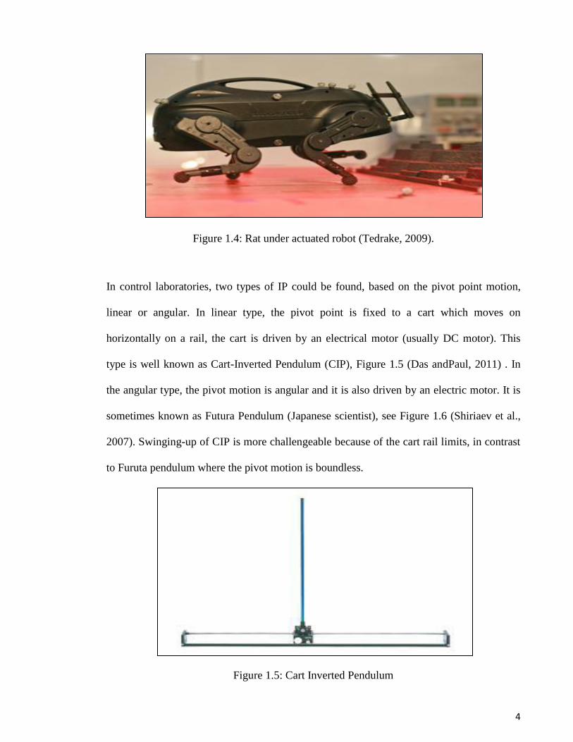
1.3 Fuzzy Logic Control
Fuzzy Logic Control (FLC) has been introduced as an alternative tool for nonlinear
complex systems. It is also known as Knowledge Based Fuzzy Control (KBFC) because of
using the human knowledge. The fuzzy control algorithm consists of linguistic expressions
in form of IF-THEN rules. The rules are designed based on the human experience and
knowledge.
Fuzzy logic and fuzzy sets were introduced by Lotfy Zadeh in 1960s (L. A. Zadeh, 1965;
Lotfi A. Zadeh, 1973). Fuzzy control process is divided into three main sequences:
fuzzification, decision making and defuzzification, see Figure 1.7. Fuzzification process
converts the real or crisp inputs value into the fuzzy value, based on the membership
functions. The controller decision is taken based on the human experience through IF-
THEN rules. Finally, in deffuzification stage, the controller output is converted back to the
physical value.
6
Figure 1.7: Fuzzy control process.
FLC control has been applied widely for many engineering applications. However, it has
some drawbacks in analyzing some complicated systems where the numbers of rules are
increased. (Passino andYurkovich, 1998). In this study, a fuzzy controller will be applied to
swing the pendulum up under the cart rail restrictions.
1.4 Sliding Mode Control
Sliding mode control technique provides a robust control tool that deals with nonlinear
systems. It was initially developed in Soviet Union during the early of 1960s (Edwards
andSpurgeon, 1998; Itkis, 1976; Utkin, 1977). Recently, sliding mode has been extensively
applied in many engineering aspects e.g., Robotics, aerodynamics and power electronic
(Liang andJianying, 2010; Siew-Chong et al., 2008; Xiuli et al., 2010).

7
The main advantages of sliding mode are: 1) Stability guarantees 2) robustness under
system parameters variation. 3) External disturbances rejection. 4) Fast dynamic response.
However, sliding mode has a drawback of chattering problem (high frequencies in the
control signal) which might cause actuators failure. Numbers of solutions have been
introduced to decrease the chattering effects (Boiko andFridman, 2005; Mondal et al.,
2012; Young andDrakunov, 1992).
The Sliding Mode Controller (SMC) design consists of two parts: the sliding surface and
the control law. The control law is designed to force the system states to move towards the
sliding surface. Once the sliding surface is reached, the system state will slide on the
surface till it reaches the stability point (Yorgancioglu andKomurcugil, 2010). In this
project, SMC is used to design a stabilization controller CIP to keep the pendulum stable in
the upward position under the effects of friction forces and external disturbances
1.5 Objectives
The main objective for this study is to design a fuzzy sliding mode controller to swing up
and stabilize the CIP system. Several objectives are set to achieve the main objective, as
follows:
1- To derive third order mathematical model, that combines the Cart-Pendulum with
its DC motor dynamics.
2- To design a fuzzy controller for swinging the pendulum up within the cart rail
limits.

8
3- To design sliding mode controller surface in order to keep the pendulum and the
cart in the stability position.
4- To test the proposed control algorithm using Matlab Simulink and Fuzzy logic tool
box.
5- To implement the controller on a real CIP system and compare the experimental
results with other linear controller techniques.
1.6 Thesis outline
The rest of thesis is organized as follows: in Chapter 2 a literature review covering former
proposed swinging-up controller for CIP has been discussed. In addition, Stabilization
controller (linear and nonlinear) has been surveyed. A Third order combining model for
cart-pendulum system with DC motor has been derived in Chapter3. The Cart-pendulum
model has been obtained based on Newton’s second law of motion. The friction between
the cart and its rail has been described with a nonlinear friction mode. The DC motor circuit
has been modeled and linked with cart-pendulum equations in the same mathematical
model.
Chapter 4 presents swinging-up and stabilization controller design. Fuzzy swing-up
controller has been designed in consideration of the cart rail limits. Sliding mode
stabilization controller has been introduced. Moreover, LQRC has been suggested in order
to be compared with the proposed sliding mode controller. In Chapter 5, CIP combining
model has been cooded in Matlab Simulink. Fuzzy swing-up controller with sliding mode
stabilization controller has been tested and simulation results have been presented. Also, the

9
swinging-up controller with LQR stabilization controller has been performed and the
results has been illustrated.
In Chapter 6, the proposed control techniques have been implemented in a real CIP system.
The experimental setup has been described and the experimental results have been shown.
A comparative study, between the proposed controller and LQR technique, has been
conducted in Chapter 7, and the results have been discussed, and the project objectives have
been evaluated. Finally, the study conclusion is presented in Chapter 8, and future work is
suggested.

10
Chapter Two
2 Literature Review
2.1 Introduction
It is known that CIP has two sub-controllers: swinging-up and stabilization. In swing up
stage, the controller is applied to swing the pendulum to the upward position under the cart
rail length limits. The more effective swing-up controller takes less time and fewer numbers
of swings. Once the pendulum reaches the upright position, it should be balanced by a
proper stabilization controller. This controller keeps the pendulum stable at the upright
position, despite friction forces and external disturbances.
For the real controller implementation, several constraints should be considered. For
example, the friction force between the cart and the rail which acts as an unknown
disturbance that affect the system stability. Also, there are limits for the maximum control
signal and the rail length. Moreover, the actuator dynamics have to be deemed for
experimental application.
In this chapter, a literature review covering CIP swinging up and stabilization controllers is
presented. The swinging-up controllers review contains the main control techniques that
have been introduced during the last two decades in order to solve the swing-up problem.
The stabilization control review is divided into two subsections: linear techniques and
nonlinear techniques. In nonlinear controller review we mainly focused on the sliding mode
control which has been developed in this work. Finally, the study plan is explained based
on the found gaps.

11
2.2 Swinging-up controllers
In literature, several Swing-up controllers have been introduced during the last two decades
to swing the pendulum system to the upward position. Starting with classical methods,
(Furuta et al., 1991) by using feed forward control method and (Furuta et al., 1992) that
used pseudo state feedback controller to swing up Futura pendulum.
New controller for swinging-up the pendulum has been developed based on the pendulum
energy, it has been known as energy control method (Åström andFuruta, 1996, 2000). In
this technique, the pendulum energy (kinetic and potential) was controlled to equal the
upward position energy. This method gives a direct relation between the maximum
acceleration of the pendulum pivot and the number of required swing. However, the pivot
velocity and position are not considered, thus makes this techniques are not applicable for
CIP where the cart rail is limited. Numbers of swing-up techniques have been proposed
based on the energy control principle such as, (Shiriaev et al., 2001) where variable
structure control version of energy based controller has been suggested to swing up the
pendulum. and (Bugeja, 2003)where swinging-up and stabilization controller based on
feedback linearization and energy considerations is proposed. However none of these
controllers have been tested on a real system.
A Sliding Mode Control law for swinging the pendulum up in one time without swinging
motion has been proposed (M. S. Park andChwa, 2009). Simulation and experimental
results show the validity for this controller for futura pendulum, where the base motion is
unlimited. A new controller based on planning trajectory was proposed and implemented

12
on a real Futura pendulum (La Hera et al., 2009). The result shows the controller
effectiveness in swining-up the system.
In (Mason et al., 2008; Mason et al., 2007), an optimal time swinging-up controller is
proposed to swing-up the pendulum. In this controller, the cart acceleration is considered to
be the system input. Therefore, this controller cannot be implemented easily, because of
neglecting of the system actuator.
Nonlinear controller has been applied in (Wei et al., 1995), where the cart rail limits are
considered. This controller needs less cart motion comparing to classical linear controllers
control laws. In (Chatterjee et al., 2002), energy well swinging-up controller is designed,
where the cart rail restrictions are considered. In addition, linear stabilization controller is
introduced to catch the pendulum in the upright position. Simulation and experimental
results show the validity for this controller. However, in the swing-up part, five different
parameters should be chosen by try and error which is not simple. More simple swinging-
up controller has been proposed by (Yang et al., 2009) with only two design parameters.
This controller shows more simplicity in tuning the controller. However, this controller has
been tested experimentally; the stabilization part has not been studied.
A simple fuzzy swinging-up controller with stabilization controller was introduced in
(Muskinja andTovornik, 2006). Simulation and experimental results confirmed the
effectiveness of the swinging-up controller comparing with energy control method.
However, the stabilization controller does not guarantee the stability because of model
linearization.

13
2.3 Stabilization controllers
Stabilization controllers of IP systems could be classified into two types: linear and
nonlinear control techniques. In linear type, the system is approximated to linear model,
where the classical control theories are applied directly. However, this kind of controller
might suffer from global instability because of the model inaccuracy due to linearization. In
nonlinear control techniques, controllers are designed based on the exact model without
approximation. These techniques are much complicated however, the system stability is
guaranteed and the system response is significantly improved comparied with linear
controllers.
2.3.1 Linear Stabilization controllers
Since 1960s, inverted pendulum was used to demonstrate linear control techniques such as
PID (Proportional Integration Derivative) and LQR (Linear Quadratic Regulator) and
Feedback Linearization (FBL) (Furuta et al., 1978; Mori et al., 1976; Sugie andFujimoto,
1994) .Generally, PID controllers are used to control SISO (Single-Input Single-Output)
systems. As CIP is considered as SIMO (Single-Input Multi-Output) system, two PID
should be used together to control the pendulum and the cart. In this type of controller, six
parameters should be selected to carefully to control the system, so that the controller
tuning quite difficult. Thus, advanced techniques like neural network are used to tune the
controller (Faizan et al., 2010) (Fallahi andAzadi, 2009; Fujinaka et al., 2000; Rani et al.,
2011). FBL controller has been proposed by (El-Hawwary et al., 2006). In order to improve
the system stability and the disturbance rejection ability, a damping term and an adaptive
fuzzy term is added. Simulation and experimental results show the validity for this
controller.

14
Linear quadratic Regulator (LQR) control technique was also used to stabilize the
pendulum system. In this scheme the pendulum system model is approximated into the
linear state space form. Afterward, the feedback gains are calculated based on the
minimum cost function this method shows better result and simple control scheme
comparing with PID (Barya et al., 2010; Prasad et al., 2011, 2012; Wongsathan andSirima,
2009) .
In order to improve the linear controller response, LQR with nonlinear friction compensator
has been proposed in (Campbell et al., 2008; D. Park et al., 2006). In these studies,
nonlinear friction compensators, based on nonlinear friction models, are used to improve
the steady state result. Simulation and experimental result showed the controller ability to
reject some oscillation which caused by friction forces.
2.3.2 Nonlinear Stabilization controllers
In order to guarantee the system stability, nonlinear control techniques has been applied to
control CIP system. In these methods, a nonlinear model is derived for the system in order
to achieve better stability comparing to linear algorithms.
New Takagi-Sugeno (T-S) fuzzy model has been proposed for CIP by (Tao, Taur, Hsieh, et
al., 2008). A fuzzy controller with a parallel distributed pole was designed to stabilize the
system. In addition, nonlinear friction model, control signal constraints and cart rail limits
were considered. Only simulation work has done to prove the controller effectiveness.
Sliding mode controller was proposed in (Tao, Taur, Wang, et al., 2008) to control CIP.
The system model was divided into two subsystems (cart and pendulum), sliding mode
controller has been proposed for each subsystem. The controller parameters were adjusted
15
by an adaptive mechanism. Simulation results showed the stability for this controller under
disturbances.
Decoupled sliding mode controller was proposed by(Lo andKuo, 1998). In this approach,
the whole system is decoupled into two subsystems (pendulum and its cart); each one has
its control target. In order to link between the two subsystems targets, an intermediate
function is designed to ensure that the control signal will control both of subsystems. The
fuzzy controller is added to overcome the chattering problem near the switching surface.
Simulation results showed that both of the pendulum angle and the cart position converge
to zero. However, this controller hasn’t considered the experimental limitation, e.g., DC
motor dynamics, friction and cart length restriction.
A hierarchical fuzzy sliding mode controller for CIP was introduced in (Lin andMon,
2005). In this approach, two subsystem controllers are designed for each system state and
an adaptive law is used to find the controller coupling parameters. Simulation results
showed the effectiveness of this controller. Neural network decoupling sliding mode
controller for CIP is introduced by (Hung andChung, 2007). The coupling between the two
subsystems has been done using the neural network. The results demonstrated the
robustness for this controller. However, in (Hung andChung, 2007; Lin andMon, 2005) the
decoupling techniques are more complicated comparing with Chang controller(Ji-Chang
andYa-Hui, 1998)and experimental verification is still needed as well.
More advanced controller based on time varying sliding surface controller is proposed in
(Yorgancioglu andKomurcugil, 2010). The sliding surface slope was computed by linear
functions which are approximated from input-output relation of fuzzy rules. Results show
improvement of the pendulum angle response in terms of speed convergence. The cart rail
limits and DC motor dynamics are not considered in their study.
16
2.4 Study plan
In this work, a new combining model, for the cart-pendulum models and its DC motor
dynamics, has been derived in third-order mathematical model. The motor control voltage
is the input variable in the obtained model. This representation is applicable for the real CIP
system. Friction forces between the cart and its rail are also considered in a nonlinear
model.
A fuzzy swinging-up controller is designed to swing the pendulum to the upward position.
Using fuzzy logic control the pendulum is swung up where the cart rail limits is considered.
Once the pendulum reaches the upward position, a sliding mode controller is designed to
keep the pendulum stable in the upward position. To reach the full system stability for the
pendulum and the cart, an intermediate function is designed to link the cart position with
the pendulum angular position. LQR controller is designed and compared with the
proposed controller. The system model, controller design, simulation and experimental
results are shown in subsequence sections.

17
Chapter Three
3 Mathematical model
3.1 Introduction
A new third order model for CIP is derived in this chapter, where the pendulum and cart
dynamic are combined with the DC motor model. The main experimental limitations such
as nonlinear friction force between the cart and the rail and the DC motor dynamics are
considered. The derived model has the advantage of joining the mechanical system (cart
and pendulum) with the electrical system (DC motor) in the same model, where the DC
motor control voltage is considered as the system input.
3.2 Pendulum model
Figure 3.1: The Cart-Pendulum system
18
CIP has two degrees of freedom, X is the Cart displacement and θ is the pendulum angle
position, as shown in Figure 3.1. The cart displacement is assumed to be positive in the
right direction, and negative in the left direction. The pendulum angle is considered to be
positive in CCW rotation, and negative in CW rotation. The free body diagram of the cart
and the pendulum are shown in Figure 3.2 and Figure 3.3 , respectively. V is the veritical
reaction force between the pendulum and the cart, H is the horizontal reaction force
between the cart and the pendulum.
X
M
F
V
H
frF
Figure 3.2: Cart free body diagram
19
Figure 3.3: Pendulum free body diagram.
The cart mass is donated by M , m is the pendulum mass, L is the length between the pivot
and the pendulum center of gravity CG, g is the acceleration of gravity, I is the pendulum
mass moment of inertia with respect to its CG, Ffr is the friction force between the cart and
the rail. q is the friction coefficient in the pendulum pivot.
Free body diagram analysis has been performed for the cart and the pendulum. For the cart
free body diagram, by takingthe equlibrium of forces in the horizontal direction and
applying Newton’s second low of motion,the following equation is obtained:
fr
M X F F H (3.1)

20
From the pendulum free body diagram, the summition of forces in the horizontal directions
is:
2( cos sin )H m X L L (3.2)
By taking forces equlibrium in the vertical direction:
2( sin cos )mg V m L L
2( sin cos )V m g L L (3.3)
By summing the moments around the pendulum center of gravity:
sin cosI V L H L q (3.4)
Substitute from (3.2) into (3.1), and from (3.2) and (3.3) into (3.4), the cart-pendulum
equations are derived:
2( ) ( cos sin )fr
F M m X F m L L (3.5)
2( ) sin cosI mL mgL mLX q (3.6)
Equations (3.5) and (3.6) are the main equations of motion for the mechanical part. As it is
noticed, the system input is the force F. This model is not applicable from practical point of
view, since the DC motor is still needed to generate the force F.

21
3.3 Friction model
Friction is a physical phenomenon which occurs in all moving mechanical systems. It is
considered as a resistive force generated between the two interacting surfaces and having a
relative motion. In control systems, the friction forces have a significant effect on the
system response, which might cause system instability. Steady state error and oscillations
are found in the system response when the friction force is neglected. In order to eliminate
such effects from the system response, the friction should be included in the system model
and controller design.
Most of the earlier work, dealing with the CIP, either has applied a viscous friction model
(linear) or has neglected its effects (Muskinja andTovornik, 2006). However, the friction
phenomena encloses many terms such as Stribeck effects, static, Coulomb and viscous
frictions (Armstrong-Hélouvry et al., 1994; Olsson et al., 1998). Thus, exponential friction
model Ffr is chosen, to address all mentioned terms of friction, as follows:
/
( ) ( )n
S
d
dC S
s
dfr
C
X V
if X X
F F F e sgn X b X if
FX
X
X X
F (3.7)
Where, FS is Static Friction force, FC is Coulumb Friction force, d is the dead zone
velocities, VS is Stribeck velocity, n is form factor, b is the viscous friction coefficient.

22
3.4 Dc Motor model
Figure 3.4: DC Motor circuit
Figure 3.4 illustrates the Dc motor Circuit, where, Va is the armature applied voltage
(Control voltage), Vemf is the back EMF voltage, Ra, La and i are the armature resistance,
inductance and current, respectively. ω is the DC Motor angular velocity, Te is the Motor
electromagnetic torque, TJ is motor inertia torque, TB is the damping torque and TL is the
motor load torque. The motor equations are
a a aemf
diV V i R L
dt (3.8)
eemfV K (3.9)
Ke is the Back EMF constant, and
e
t
Ti
K (3.10)
Kt is the motor torque constant. The relation between the cart linear velocity and the motor

23
angular velocity is given by ((3.11).
X
r (3.11)
r is the motor pulley diameter. The electromagnetic torque equation will be
e J B LT T T T (3.12)
Where
J
XT J J
r (3.13)
B
XT B B
r (3.14)
L
T F r (3.15)
J is the motor rotor mass moment of inertia, B Motor rotor damping coefficient.
3.5 Overall system model
Here, two third differential equations will be derived to describe the overall system, where
the motor applied voltage Va is the system input. By substituting from (3.13), (3.14) and
(3.15) in (3.12). And from (3.12) in (3.10) we get the current equation

24
2
[( )
( cos sin )]
e
t t
fr
t
X XJ B M m X
T r riK K
F m L L r
K
(3.16)
Taking the time derivative of the current equation, (3.17) is obtained
(3.17)
By substituting from (3.9), (3.16) and (3.17) into (3.8), we get
2
3
sin
[( ) ] [( ) ] [ ]
[ ] [ ] cos
3cos sin cos
] ]
]
[ [
[ a
t
a a aa
t t t
a e a
t t
a a a
t t t
a afr fr
t t
r m LR
K
L R B LJ JV M m r X M m r X
r K r K r K
B R K r m LRX
r K r K
r m LL r m LL r m LL
K K K
R LF F
K K
(3.18)
Equation (3.18) is considered as the main overall equation, describing the system states
with the applied voltage on DC motor as an input. From (3.6) we can get;
2( )tan
cos cos
I mL qX g
mL mL (3.19)
3
[( ) ] cos
sin 2 sin cos
t
fr
t
J BM m r X X m Lr
di r rdt K
m Lr mLr m Lr F
K

25
2 2 2
sin cos( ) ( ) ( )
mLg mL qX
I mL I mL I mL (3.20)
Differentiate one more time,
2( )tan
cos cos
q I mLX g X
mL mL (3.21)
2 2
2 2
cos cos( ) ( )
sin( ) ( )
mgL mLX
I mL I mL
mL qX
I mL I mL
(3.22)
Substituting from (3.19) and (3.21) into (3.18), we get the pendulum angle third order
differential equation.
313 14 15 16
21
22
4 5 73 6
21
28 9 10 11 12
21
21
sin cos
[ cos ]cos
tan tantancos cos cos
[ cos ]cos
tan cos sincos
[ cos ]cos
1
[ cosc
fr frf f f F f F
ff
f f f f f
ff
f f f X f f
ff
ff
]
os
aV
(3.23)

26
Where the values of constants f1→16 are:
1
a
t
r m L Lf
K,
2
2
[( ) ] [ ]a
t
JM m r L I mL
rfK m L
,
3
[( ) ]a
t
JM m r L g
rfK
4
[( ) ]a
t
JM m r L g
rfK
,
2
5
[( ) ] [ ]a
t
JM m r L I mL
rfK m L
,
6
[( ) ]a
t
JM m r L q
rfK m L
2
7
[( ) ] [ ( ) ] [ ] )] ([ a
a a
t
B LJ JM m r L q M m r R
r r rf
K m L
I mL
8
[( ) ] [ ] ][ a a
t t
R B LJf M m r g
r K r K
9
[( ) ] [ ] ][ a
a
t
B LJM m r R
r rf
K m L
q
,
10
[ ] [ ] ][ a e
t
B R Kf
r K r, 11
a
t
r m LRf
K,
12
a
t
r m LRf
K
13
3a
t
r m L Lf
K,
14
a
t
r m L Lf
K
15
a
t
Rf
K,
16
a
t
Lf
K
Equation (3.21) is rewritten in the form:
1 1( , , , ) (( , , , ) aX X X X V (3.24)

27
Where,
7 8 9 10 11
21
22
4 53 6
21
2 312 13 14 15 16
21
1
tan coscos cos
[ cos ]cos
tan tantan
cos cos
[ cos ]cos
sin sin cos
[ cos ]cos
fr fr
f f f f X f
ff
f f f f
ff
f f f f F f F
ff
(3.25)
1
21
1
[ cos ]cos
ff
(3.26)
Similarly to get the cart position third order differential equation, substitute from (3.20) and
(3.22) into (3.18)
2 24 53 6
22 1
2 27 8 9 10 11 12
22 1
313 14 15
22 1 2
cos sin cos cos sin cos
[ cos ]
cos sin sin sin cos
[ cos ]
cos 1
[ cos ] [ cfr fr
f f X f f XX
f f
f f X f X f f f X
f f
f f F f F
f f f 21os ]
aVf
(3.27)
28
Where the values of constants f ′1→15 are:
1
[( ) ] a
t
JM m r L
rfK
,
2 2
2 2( )a
t
r m L Lf
I mL K,
2 2
3 2( )a
t
r m L L gf
I mL K
2 2
4 2( )a
t
r m L L gf
I mL K ,
2 2 2 2
5 2 2 2( ) ( )a a
t t
r m L L q g r m L R gf
I mL K I mL K
2 2 2 2
6 2 2 2( ) ( )a a
t t
r m L L q r m L Rf
I mL K I mL K ,
2
7 2 2 2( ) ( )a a
t t
r m LL q r m LR qf
I mL K I mL K
8
[( ) ] [ ] ][ a a
t t
R B LJf M m r
r K r K,
9 [ ] [ ] ][ a e
t
B R Kf
r K r ,
10 2
3
( )a a
t t
r m LR r m LL qf
K I mL K
2 2
11 2
3
( )a
t
r m L L gf
I mL K ,
2 2
12 2
3
( )a
t
r m L Lf
I mL K , 13
a
t
r m LLf
K , 14
a
t
Rf
K , 15
a
t
Lf
K
Equation (3.27) is rewritten in the form:
2 2( , , , ) ( , , , ) aX X X X X V (3.28)

29
Where,
2
3 4 52 2
2 1
2 2
6 7 8 9 10
2
2 1
2 3
11 12 13 14 15
2
2 1
cos sin cos cos sin
[ cos ]
cos cos sin
[ cos ]
sin sin cos cos
[ cos ]fr fr
f f X f
f f
f X f f X f X f
f f
f f X f f F f F
f f
(3.29)
2 2
2 1
1
[ cos ]a
Vf f
(3.30)

30
Chapter Four
4 Methodology
4.1 Introduction
Methodology of Swinging-up and stabilization control is discussed in this chapter. For the
pendulum swinging-up, fuzzy logic controller is designed to achieve the task in
consideration of the cart rail limits. After reaching the upward position, SMC is developed
to guarantee the system stability. Linear control technique (LQRC) is designed, in order to
be compared with the proposed SMC. The controller schematic diagram is shown in
Figure4.1.
Figure4.1: schematic diagram for Swing up with stabilization controller.
4.2 Fuzzy swing-up controller
The main idea of the fuzzy swinging–up controller is based on the pendulum energy, which
equals the summation of its kinetic and potential energies(Åström andFuruta, 2000). By

31
controlling this energy, and raise it to equal the upward position energy, the pendulum
could be swung-up. The pendulum energy E is given by
2 cosPE I m g L (4.1)
Where, IP is the pendulum mass moment of inertia around the pivot point. According to
(4.1), the pendulum energy depends on the pendulum angle and the pendulum angular
velocity. In other words, the pendulum energy can be increased by controlling the variables
θ and θ . The cart rail limit should be also considered in swinging-up thus, for the fuzzy
controller, three input variables are chosen: the pendulum angle θ, the pendulum angular
velocity θ and the cart displacement X. The DC motor control voltage Va is the output
variable.
Figure 4.2: Membership functions of the pendulum angle.

32
Figure 4.3: Membership functions of the pendulum angular velocity.
As it is shown in Figure 4.2, five membership functions (1, 2, 3, 4 and5) are chosen for
the pendulum angle. Note that the rectangular membership function (1) represents the
pendulum angle if (π/2 ≤θ < 3π/2), where, the accurate pendulum angle measurement is
not required. The other four membership functions are chosen to be in a triangular shape
because they are located near to the upward position, where more accurate measurement
is needed. In Figure 4.3, the pendulum angular velocity is represented by two membership
functions N (counter clock wise) and P (clock wise) as illustrated. The cart displacement
is represented by two triangular (P and N) and one trapezoidal (Zero) membership
functions (Zero) as shown in Figure 4.4. For the output control voltage, seven singleton
membership functions are selected in Figure 4.5, to represent the applied control voltage
on the DC motor. The singleton membership functions positions are chosen to minimize
the swinging-up time.

33
Figure 4.4: Membership functions of the cart position.
Figure 4.5 : Membership functions of the output control voltage.

34
The swing-up controller is designed based on 30 fuzzy rules. The rules conse uents are
chosen to increase the pendulum energy to reach the upward position energy. During the
swinging-up, the cart rail limitation should be considered. ach three rules are designed at
the same endulum angle θ and angular velocity θ , with consideration of the cart position.
For instance, if the pendulum angle is 1 and the pendulum angular velocity is N, the three
rules are developed as follows: First, without consideration of the cart limits, the logical
swing-up control action should be . Then, the cart position membership functions (N,
and ero) will be considered to form the three rules, for each rule θ and θ are constant (1
and N, respectively).
Rule1:
f θ is and θ is N and X is P, then Va(swing-up) is Zero.
It means that the pendulum is located in the downward half cycle (π/2 ≤ θ < 3π/2) and it
rotates in CW direction. As it is mentioned above, the logical swing-up control decision
should be PB. Since the cart is located at the positive side of the rail (X is P).Thus, In order
to keep the cart within the limits, and the rule consequent should be Va(swing-up) is Zero.
Rule 2:
f θ is and θ is N and X is Zero, then Va(swing-up) is PM.
For this rule the cart is located in the middle of the rail (X is Zero). Thus, the control action
will be chosen to move the cart in the positive direction, but with a medium force, and the
rule consequent will be Va(swing-up) is PM.

35
Rule 3:
f θ is and θ is N and X is N, then Va(swing-up) is PB.
Because the cart is located at the rail negative side (X is N), the the rule consequent will be
kept Va(swing-up) is PB
The rest 27 rules are chosen with the same procedures. This controller allows the pendulum
to reach the upward position while the cart remains within the restricted limits. The fuzzy
swing-up rules are as follows:
Rule 4: f θ is and θ is P and X is P, then Va(swing-up) is NB
Rule 5: f θ is and θ is P and X is Zero, then Va(swing-up) is NM
Rule 6: f θ is and θ is P and X is N, then Va(swing-up) is Zero
Rule 7: If θ is 2 and θ is N and X is P, then Va(swing-up) is NB
Rule 8 : f θ is 2 and θ is N and X is Zero, then Va(swing-up) is NM
Rule 9: f θ is 2 and θ is N and X is N, then Va(swing-up) is Zero
Rule 10: f θ is 2 and θ is P and X is P, then Va(swing-up) is Zero
Rule 11 : f θ is 2 and θ is P and X is Zero, then Va(swing-up) is PM
Rule 12: f θ is 2 and θ is P and X is N, then Va(swing-up) is PB
Rule 13: f θ is 3 and θ is N and X is P, then Va(swing-up) is NB
Rule 14: f θ is 3 and θ is N and X is Zero, then Va(swing-up) is NM
Rule 15: f θ is 3 and θ is N and X is N, then Va(swing-up) is Zero
Rule 16: f θ is 3 and θ is P and X is P, then Va(swing-up) is Zero
Rule 17: f θ is 3 and θ is P and X is Zero, then Va(swing-up) is PM

36
Rule 18: f θ is 3 and θ is P and X is N, then Va(swing-up) is PB
Rule 19: f θ is 4 and θ is N and X is P, then Va(swing-up) is NM
Rule 20: f θ is 4 and θ is N and X is Zero, then Va(swing-up) is NS
Rule 21: f θ is 4 and θ is N and X is N, then Va(swing-up) is Zero
Rule 22: f θ is 4 and θ is P and X is P, then Va(swing-up) is Zero
Rule 23: f θ is 4 and θ is P and X is Zero, then Va(swing-up) is PS
Rule 24: f θ is 4 and θ is P and X is N, then Va(swing-up) is PM
Rule 25: f θ is and θ is N and X is P, then Va(swing-up) is NM
Rule 26: f θ is and θ is N and X is Zero, then Va(swing-up) is NS
Rule 27: f θ is and θ is N and X is N, then Va(swing-up) is Zero
Rule 28: f θ is and θ is P and X is P, then Va(swing-up) is Zero
Rule 29: f θ is and θ is P and X is Zero, then Va(swing-up) is PS
Rule 30: f θ is and θ is P and X is N, then Va(swing-up) is PM
Note, the swing-up time could be controlled by selecting the output voltage (Va)
membership functions. In the real application, the swing-up time also depends on the DC
motor maximum voltage.
The control output value has been utilized by center of gravity defuzzification method. The
fuzzy controller uses the following equation has been used to obtain the real control output
max
min
max
min
( ).
( )
x
x
x
x
x x dx
CoA
x dx
Where CoA is the center of area which represents the control output, x is value of linguistic
variable, xmax and xmin are the linguistic variable range. μ(x) is the variable membership.

37
4.3 Sliding Mode stabilization controller
Sliding Mode Controller is designed based on the third order derived mode. From the
system model in (3.24) and (3.28), and if D1and D2 are bounded external disturbances, the
entire system model will have the following form
11 1 a DV (4.2)
22 2 a DX V (4.3)
Where, α1 and β1 are nonlinear functions of the system states θ θ and θ . α2 and β2 are
functions of θ θ and . The control law is designed based on the sliding surface. The
general equation of the sliding surface S is (Bartoszewicz andNowacka-Leverton, 2010;
Palm et al., 1997)
1( , ) .)( nd
S x t C xdt
(4.4)
Where x is the system sate, n is the system order and C is a constant value. In this case
(CIP) the system states are θ θ θ , X, and . Thus, two sliding surfaces, S1 for the
pendulum subsystem and S2 for the cart subsystem, are considered. Where
2
1 1 12S C C (4.5)
38
2
2 2 22S C X C X X (4.6)
C1 and C2 are positive constants. Sliding surfaces S1 andS2 are constructed based on the
constants C1 and C2. Appropriate selection of these constants values will achieve the
desired response.
The control law is designed based on the sliding surfaces. Since only one control action is
available, the Pendulum angle will be considered as primary control target and the cart
position is the secondary target. Initially, the controller is designed to achieve the primary
target where S1 = 0. An intermediate function is used to link between the secondary and
primary targets. This function will achieve the cart subsystem stability if the pendulum
stability is reached. The control law is designed based on Lyapunov like function V
2
1
1
2V S (4.7)
As it is known from sliding mode theorem, in order to achieve the system stability the
control law must match the following reaching condition
1 1 1V S S S (4.8)
Where η > 0, this condition ensures that the system will be driven into the sliding mode.
The control law will be derived as follow, from (4.8)
11.sgn( )S S (4.9)
Taking the first derivative for (4.5)
21 1 1 ( 2 )S C C (4.10)

39
Substituting with (4.10) in (4.9)
2
1 1 1 11 1( 2 ).sgn( )aC C D SV (4.11)
2
1 1 1 1 11 1( 2 ).sgn( ) .sgn( )aC C D S SV (4.12)
2
1 1 1
1 11
1 11 1
2( ).sgn( ) .sgn( )a
C C DS SV
(4.13)
From (4.13), the control law could be written in form
2
1 1 1
( ) 1 1
1
2sgn( )
a stablize
C CV K S (4.14)
Where
1
1
KD
The first term of the control law is estimated from the system model, and it will be donated
as a(stabilize), where
2
1 1 1
( )
1
2ˆa stablize
C CV
40
This form of the control signal guarantee the stability for the pendulum subsystem since the
reaching condition is achieved and the sliding motion will occur. The control action Va , as
it is shown in (4.14), has a high-frequencies switching because of the Sgn function. To
overcome this problem, a boundary layer will be formed by replacing Sgn function with Sat
function as follows,
1 1( ), 0a a
SV V K Sat where (4.15)
Where
1 1 1 1
1 1 1 1
1 1
, 1
,
( )
1S S
Sgn
SatS S
if
if
S (4.16)
This kind of control will be capable of rejecting all the high-frequencies and solve the
chattering problem.
The control law in equation (4.15) can only guarantee the pendulum angle stability. The
control objective is to move the pendulum and the cart subsystems to the sliding surfaces S1
and S2, respectively, where the overall system stability could be achieved. In order to do
that, an intermediate function Z has been introduced to link between the two subsystems
sliding surfaces S1 and S2. The function Z design is introduced as follows:
First, the first sliding surface will be reformed to be
2
1 1 1( ) 2S C Z C (4.17)

41
Where, Z is a function of S2 which means that the sliding surface S2 was incorporated into
the sliding surface S1 through Z function. The new sliding surface has changed the control
target from θ=0, θ =0 and θ =0 to θ=Z, θ =0 and θ =0. The objective (S2 = 0) is now
embedded in the main control target through the variable Z which is defined
2( ). U
z
SZ sat Z (4.18)
Where, ZU is the upper limit of the function; ΦZ is the function boundary layer. Z is
abounded oscillatory function decays to zero. When Z reach zero, S1 will be zero according
to (4.17). (Yorgancioglu andKomurcugil, 2010).
In order to prove that Z is a decaying function, from equation (4.17), if we defined θ as x1,
θ as x2 and θ as x3. The controller guarantees that the pendulum subsystem moves towards
the sliding surface S1=0. Equation (4.17) could be written in the form:
2
1 1 1 1 2 3( ) 2 0S C x Z C x x
By taking the second derivative:
2
1 1 1 1 2 3( ) 2 0S C x Z C x x
2
1 1 1 3 33( ) 2 0S C x Z C x x

42
The equation could be rearranged to be
2 2
3 1 3 1 132x C x C x C Z
This considered as a linear nonhomogenous second order differential equation. The general
solution for x3 will be
1 12
3 3 3 1 3 1
0 0
( ) (0) (0) (0) ( )
t t
C t C tx t x x C x t e C e Z d dt
Where x3(0) and x3 (0) are the initial conditions (at t=0).
The first term in the right side is the complementary solution which comes from solving the
homogenous part, whereas the second term is the particular solution which comes by
solving the nonhmogeneous part. In the steady state x3=0, which is could be achieved only
if the second term in the right side converges to zero. That will happen if only Z decays to
zero.
4.4 LQR stabilization controller
LQR control technique is widely used for linear control applications. For CIP, many LQR
controllers are designed based on the linearized system model. A six order linear model
(two third order linear equation) is expected after linearizing the system equations (3.24)
and (3.28)(Elsayed et al., 2013).However, for comparison purposes, and by neglecting the
motor induction, we derived a forth order CIP model (two second order linear equations)
like the derived models in (Chatterjee, et al., 2002; Muskinja andTovornik, 2006).

43
From equations (3.24) and (3.28) and by neglecting the motor inductance (La=0) and
linearizing the system equation around the upward equilibrium point where (θ=0). If the
pendulum was assume to move only few degrees around the upward position, where
θ=0 θ=θ θ θ=0. Equations (3.24) and (3.28) will have the following forms:
6 5 7 5 8 5 5
( / ) ( / ) ( / ) (1/ )a
g g X g g g g g V (4.19)
2 1 3 1 4 1 1
( / ) ( / ) ( / ) (1/ )a
X g g X g g g g g V (4.20)
Where
2 2 2
1[ / ][( ) ( / ( ))]
a mg R r K M m m L I mL , 2
[( / ) ( / )]a m e
g R r b K K r
2 2 2
3[( ) \ ( ( ))]
a mg R r m L g K I mL ,
2
4[( ) \ ( ( ))]
a mg R r m L q K I mL
2
5[ / ][( ) (( )( ) / ( ))]
a mg R r K mL m M I mL mL , 6
[( / ) ( / )]a m e
g R r b K K r
7[ ( )] / [ ]
a mg R r g M m K
, 8[ ( )] / [ ]
a mg R r q M m m L K
Equations (4.19) and (4.20) are the overall system linear equation. For designing LQR
controller, the system equations should be in the state space form. If the system states
vector is = θ θ ], the general state-space form is

44
x Ax Bu (4.21)
Where, x is state matrix (1x4), u control signal matrix (1x1), A is state parameters matrix
(4x4), B is control signal parameters matrix (1x4). Since only one control action (DC motor
voltage) is available, u = Va. The equivalent state-space linearized system equation is
2 1 3 1 4 1 1
5 7 5 5 56 8
0 1 0 0 0
0 ( / ) ( / ) ( / ) (1/ )
0 0 0 1 0
0 ( / ) ( / ) ( / ) (1/ )
a
X X
g g g g g gX gXV
g g g g g g g
(4.22)
From LQR theory, the following sate feedback control law is applied.
a Lu V K x (4.23)
Where K is the optimal feedback gain matrix required to get a minimum performance
index J
0
( )T TJ x Qx u R u dt
(4.24)
Where Q and R are a real symmetric matrices which are chosen by the designer. The gain
matrix KL is calculated by solving Reduced-matrix Riccati equation (4.25), after obtaining
matrix P.
1 0T TA P PA PBR B P Q (4.25)
Where P is an intermediate matrix used to calculate the gain matrix K (Ogata, 2002)

45
1 T
LK R B P (4.26)
The controller parameter Q should be carefully chosen based on the states priority. Form a
control point of view, the pendulum angle is much more important than the cart position X.
Therefore, a bigger value should be chosen for the angle element in Q matrix. Selection of
R matrix value depends on the control signal constrains. Based on the values of Q and R,
the feedback gain matrix KL is obtained.
4.5 Switching between swinging-up and stabilization control
In order to switch between the swinging-up and stabilization controllers, one-move switch
is developed. This switch ensures the fuzzy swinging-up controller will be activated only
one time. Once the pendulum reaches that upward point, the stabilization controller will be
activated permanently. The switch output (Va) could be represented as follows
( )
( )
(0 2 ), ( 1)
( 2 0), ( 1)
a swing up
a
a stablize
V if and NV
V if or or N
Where, N is an integer counter which counts the numbers of the upward position, at (θ = 0).

46
Chapter Five
5 Simulation results
5.1 Introduction
CIP system dynamics, given by the equations (3.24) and (3.28), have been solved and
simulated using MATLAB Simulink. In cooperation with Fuzzy Logic toolbox, the fuzzy
swinging-up controller is designed applied to swing the pendulum to the upward position.
Two stabilization control (sliding mode and linear quadratic regulator) schemes are
implemented and compared. Both controllers (SMC and LQRC) are tested in corporation
with the fuzzy controller in the swinging–up phase. For testing purpose, nonlinear friction
force between the cart and the rail is considered according to equation (3.7). This force is
acting as an external disturbance on the controller. The cart rail limit is ±0.4m and the
motor saturation voltage is ±6 Volt. All CIP parameters and friction forces coefficients are
listed in Table 5.1. The controller parameters, for SMC and LQRC, have been chosen to
achieve fast response. DC motor saturation voltage has been also considered in the
controller parameters selection. For SMC, the controller parameters are chosen to be
C1=5.5 C2=3.1 K=15 Φ = 8 104 Φz =19 and Zu=0.98 .and for LQRC the selected
parameters are R=diag [400 1 2500 1], Q= 4 and the generated feedback gain vector KL=
[-10 -12.9 90.5 17.4].

47
Table 5.1: system parameters
Parameter Value Unit
M 0.882 kg
m 0.32 kg
L 0.3302 m
I 7.88x10⁻⁸
kg.m2
g 9.8 m/s2
q 0.0001 N.s/rad
La 0.18 x10⁻³
H
Ra 2.6 Ohm
J 3.9 x10⁻⁷
kg.m2
B 8x10⁻⁷
N.m.s/rad
Kt 0.00676 N.m/A
Ke 0.00676 V.s/rad
r 6.35x10⁻³
m
Fs 0.1 N
Fc 0.08 N
Vs 0.1 m/s
b 1.3 N.s/m
n 4 -
d 0.05 m/s
5.2 Fuzzy swinging-up with SMC stabilization
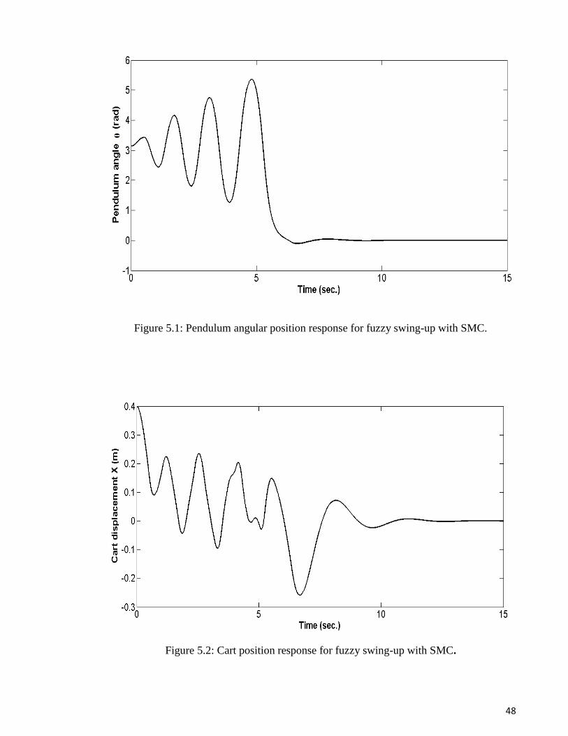
Pendulum angle response for fuzzy swing-up with SMC is shown in Figure 5.1. It is seen
that the pendulum is swung-up from downward position, where θ=π rad, into the upward
position, where θ=0. The pendulum is swung up within 6 seconds before the controller is
switched to activate the SMC. The figure shows the effectiveness of the SMC to stabilize
the pendulum, in spite of nonlinear friction forces. The cart displacement response is shown
in Figure 5.2. As it is noticed, the cart starts from the rail edge, where x= 0.4 m , and it is
kept within the rail limits before it is driven to the stability position . Figure 5.3 shows the
control signal response, where it decayed into zero.
48
Figure 5.1: Pendulum angular position response for fuzzy swing-up with SMC.
Figure 5.2: Cart position response for fuzzy swing-up with SMC.

49
Figure 5.3: Control voltage response for fuzzy swing-up with SMC.
5.3 Fuzzy swinging up with LQR stabilization controller
Pendulum angular position response under fuzzy Swing-up together with LQRC is shown
in

50
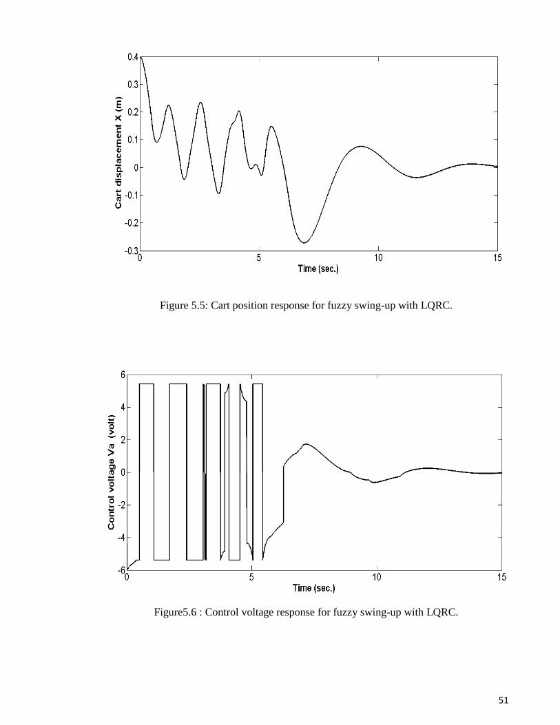
Figure 5.4. It is could be seen that the pendulum is swung up within 6 seconds before it is
balanced in the upward position. The cart response is shown in Figure 5.5, where some
oscillations could be noticed in the steady state response. Figure5.6 illustrates the control
signal curve, where the system doesn’t achieve the stability within the simulation time.
Due to friction uncertainties and system nonlinearity, LQRC could not achieve the full
stability for CIP.
Figure 5.4: Pendulum angular position response for fuzzy swing-up with LQRC.
51
Figure 5.5: Cart position response for fuzzy swing-up with LQRC.
Figure5.6 : Control voltage response for fuzzy swing-up with LQRC.

52
Chapter Six
6 Experimental results
6.1 Introduction
Simulation results have shown the proposed SMC validity to stabilize CIP under the
friction forces effects. Simulation might not be enough to prove the controller effectiveness.
Since there are many several physical parameters could not considered in the dynamic
model e.g., backlash effects between the pinion of the DC motor and the rack, also the air
drag force that acting on the pendulum motion, wear and viscoelastic deformation in the
pinion and the temperature change. In the experimental work all theses limitation and the
friction force are considered as system uncertainties. In this chapter, the proposed SMC is
tested and compared with LQR experimentally.
6.2 Experimental setup
6.2.1 Electro- mechanical setup
The experimental work has been performed with CIP model IP02 supplied by Quanser
Limited, see Figure 6.1. The electromechanical setup consists of the cart-pendulum
mechanical setup, DC motor and two incremental encoders. The encoders are used for
sensing the pendulum angular position and the cart position with a resolution of 0.0015
rad/count and 2.275x10⁻⁵
m/count, respectively. The cart slides on a stainless steel rod

53
using a linear bearing and it is driven by the DC motor via rack and pinion mechanism, as it
is shown in Figure 6.2.
Figure 6.1: CIP model IP02
Figure 6.2: CIP cart with DC motor.

54
6.2.2 Real time controller setup
The controller setup contains Personal Computers (PC) and AD/DA data accusation card
(model Q8, 14 bit with encoder inputs). The acquisition card is supplied with a terminal
board where the encoders are connected directly, as it is shown in Figure 6.3. The Control
algorithms are realized with Matlab Simulink, Fuzzy logic tool box and QuaRC real-time
toolbox developed by Quanser, with clock frequency 1 kHz. The output control signal is
amplified by Quanser power module (model UPM 800) in order to be applied directly on
the DC motor, see Figure 6.4.
Figure 6.3: AD/DA card terminal board
To Power
module
From
Encoders
To/From
AD/DA Card

55
Figure 6.4: Power module.
6.2.3 Velocity and acceleration estimation
The sensed values of the pendulum angular position and the cart position suffer from
quantization errors due to encoder’s measurements. The errors values will be enlarged in
velocity and acceleration estimation, and affect the controller results (Han et al., 2007) .
Thus, least square fitting algorithm is used to estimate velocities and acceleration for the
cart and the pendulum. The velocity and acceleration values are estimated by a third order
polynomial function. This function is established based on a least square fitting to the most
From AD/DA
Card Terminal
board
To DC Motor

56
recent 8 measured values of the encoder counts. This fitting technique is also known as
(LSF 3/8)(Brown et al., 1992). Schematic diagram for the fitting process is shown in
Figure 6.5 , where ΔT is the sampling time and T1→8 is the time for each sample.
Figure 6.5: Schematic diagram for the fitting process.
6.3 Fuzzy swinging with SMC experimental results
For SMC real time implementation, the controller parameters are chosen to be C1=4, C2=2,
K= , Φ = 2.2x 03, Φz =4 and Zu=0.9 . Figure 6.6-Figure 6.8 show the real implementation
of fuzzy swing-up and with SMC. The pendulum is swung up within 6 seconds before the
SMC is applied. The pendulum is balanced in the upward position where the stability could

57
be noticed. The cart displacement and control signal are driven near to the equilibrium
point with small oscillation.
Figure 6.6: Experimental result for pendulum angular position with Fuzzy swing up and
SMC.
Figure 6.7:. Experimental result for cart position for Fuzzy swing up with SMC.

58
Figure 6.8: Experimental result for control voltage for Fuzzy swing up with SMC.
6.4 Fuzzy swinging with LQR experimental results
For LQRC, the selected controller parameters are, R=diag[400 1 2500 1], Q= 1 and the
generated feedback gain vector KL=[-20 -21.6 124.96 23.2]. In Figure 6.9, the fuzzy
swing-up is tasted with LQRC, the results show that the pendulum takes 6 second to reach
the upward position, before the stabilization LQRC is applied. For the steady state
response, some oscillations could be noticed in the pendulum angle response because of the
friction effects and other uncertainty sources. In Figure 6.10, the cart response shows
oscillations and steady state error. Figure 6.11 shows the control signal for LQRC, where a
high overshoot values could be seen.

59
Figure 6.9: Experimental result for pendulum angular position with Fuzzy swing up with
LQRC.
Figure 6.10: Experimental result for cart position with Fuzzy swing up with LQRC.

60
Figure 6.11: Experimental result for control voltage for Fuzzy swing up with LQRC.

61
Chapter Seven
7 Comparison results and discussion
7.1 Introduction
A comparison study has been performed between the proposed SMC and LQRC. The aim
of this comparison is to show the SMC effectiveness in achieving the stability under
external disturbances, and in the real implementation. This comparison also shows the
robustness of the proposed controller comparing with other published techniques
(Chatterjee, et al., 2002; Muskinja andTovornik, 2006).
7.2 Simulation comparison
In order to test the controller robustness, an external disturbance, with value of 0.1 rad and
one second duration, has been applied after 20 seconds. The pendulum and cart responses
are shown in Figure 7.1 and Figure 7.2, respectively. The pendulum angular response
shows faster response for SMC and ability to reject the disturbance much more efficiently
than LQRC. The maximum overshoot has been reduced by 30% when SMC is applied. The
cart response shows the robustness of the SMC over LQRC where the maximum overshoot
has been increased by 100% using LQR instead of SMC. Furthermore, in LQRC, the cart
has exceeded the rail limits.

62
Figure 7.1 : Pendulum angular position response under disturbance.
Figure 7.2: Cart position response under disturbance.
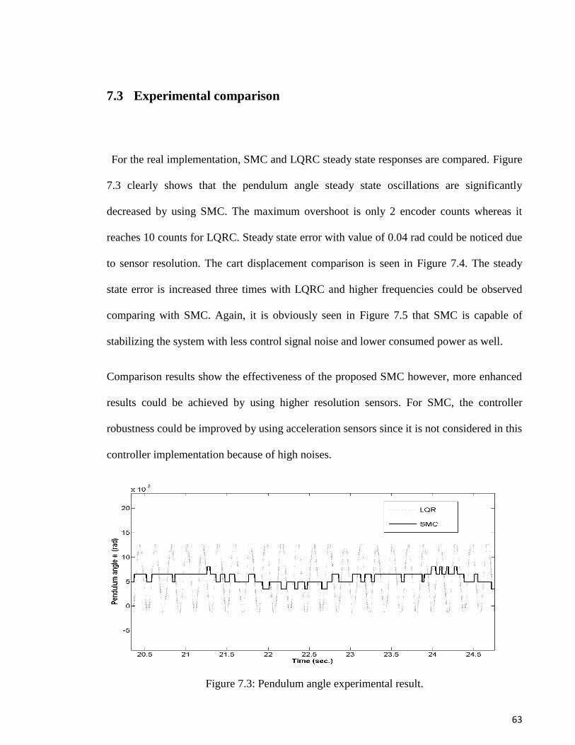
63
7.3 Experimental comparison
For the real implementation, SMC and LQRC steady state responses are compared. Figure
7.3 clearly shows that the pendulum angle steady state oscillations are significantly
decreased by using SMC. The maximum overshoot is only 2 encoder counts whereas it
reaches 10 counts for LQRC. Steady state error with value of 0.04 rad could be noticed due
to sensor resolution. The cart displacement comparison is seen in Figure 7.4. The steady
state error is increased three times with LQRC and higher frequencies could be observed
comparing with SMC. Again, it is obviously seen in Figure 7.5 that SMC is capable of
stabilizing the system with less control signal noise and lower consumed power as well.
Comparison results show the effectiveness of the proposed SMC however, more enhanced
results could be achieved by using higher resolution sensors. For SMC, the controller
robustness could be improved by using acceleration sensors since it is not considered in this
controller implementation because of high noises.
Figure 7.3: Pendulum angle experimental result.
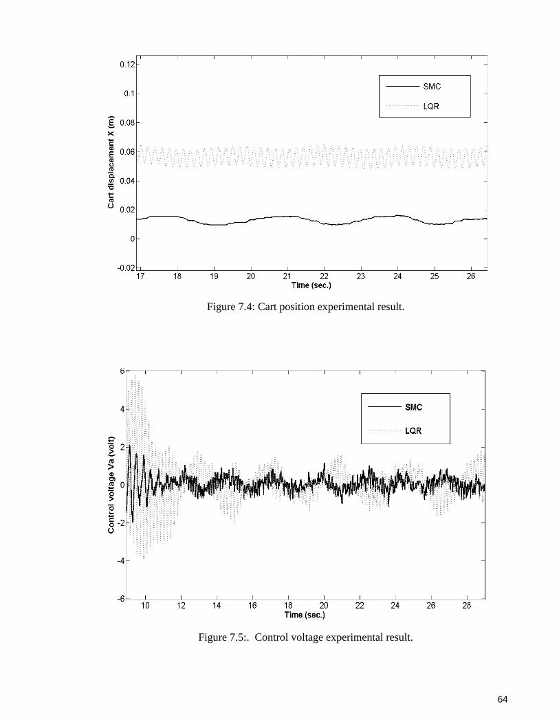
64
Figure 7.4: Cart position experimental result.
Figure 7.5:. Control voltage experimental result.
65
Chapter Eight
8 Conclusion and Future work
8.1 Conclusion
In this study, fuzzy swing-up with sliding mode controller has been developed for
swinging up and stabilization the cart-inverted pendulum system. In the system model, two
third order differential equations have been derived to combine the DC motor dynamics
with CIP mechanics in one model. For testing purpose, nonlinear friction force between the
cart and the rail has been added to the model equation. A fuzzy swing-up controller is
designed to swing the pendulum within the cart rail limits. The proposed controller is
designed based on 30 fuzzy (If-Then) rules, where the controller inputs are the pendulum
angle, the pendulum angular velocity and the cart position. Whereas, the output is the DC-
motor applied voltage. Once the pendulum reaches the upward position, the control
algorithm gives a trigger signal to one-move switch to switch between the swinging-up and
stabilization states. For system stabilization, SMC has been designed based on the derived
model, where the overall system stability is guaranteed. For comparison purposes, LQRC
has been designed to be compared with the proposed SMC.
Simulation results reviled that, the proposed SMC is effective and robust. The controllers
have been applied on a real CIP system and tested experimentally. The experimental results
have shown a significant improvement for SMC in terms of system stability, steady state

66
error and steady state oscillations. The cart position steady state error was decreased by
60% with low frequencies oscillation when applying SMC in place to LQRC.
8.2 Future work
Although the proposed SMC meets the study objectives, some points might be considered
for future investigation.
The experimental results could be improved by using accelerometers for acceleration
sensing in order to decrease the acceleration noise, since the accelerations have been
estimated based on least square fitting for the encoder counts.
The proposed controller could be generalized and applied on any two degrees of freedom
underactuated robots, two wheel mobile robot and any multi-degree of freedom under
actuated system. In addition the controller the controller might be extended to be applied on
a double inverted pendulum system.
Other control algorithm like neuro-fuzzy control might be applied and compared with the
proposed SMC. For implementation, low cost DSP real time controller instead of the real
time PC.

67
References
Armstrong-Hélouvry, B., Dupont, P., & De Wit, C. C. (1994). A survey of
models, analysis tools and compensation methods for the control of
machines with friction. Automatica, 30(7), 1083-1138.
Åström, K. J., & Furuta, K. Swinging up a Pendulum by Energy Control. 13th
IFAC World Congress, San Francisco, USA
Åström, K. J., & Furuta, K. (2000). Swinging up a pendulum by energy
control. Automatica, 36(2), 287-295.
Bartoszewicz, A., & Nowacka-Leverton, A. (2010). ITAE Optimal Sliding
Modes for Third-Order Systems With Input Signal and State
Constraints. IEEE Trans. Autom. Control, 55(8), 1928-1932.
Barya, K., Tiwari, S., & Jha, R. Comparison of LQR and robust controllers
for stabilizing inverted pendulum system. EEE International Conference
on Communication Control and Computing Technologies (ICCCCT),
2010 7-9 Oct. 2010
Boiko, I., & Fridman, L. (2005). Analysis of chattering in continuous sliding-
mode controllers. IEEE Transactions on Automatic Control, 50(9),
1442-1446.
Brown, R. H., Schneider, S. C., & Mulligan, M. G. (1992). Analysis of
algorithms for velocity estimation from discrete position versus time
data. IEEE Trans. Ind. Electron., 39 11-19.
uckingham, R. (2003). “Super mechano systems”–a report on the IEE
Tustin/UKACC annual lecture given by Professor Katsuhisha Furuta.
Industrial Robot: An International Journal, 30(5), 417-421.
Bugeja, M. Non-linear swing-up and stabilizing control of an inverted
pendulum system. EUROCON 2003. Computer as a Tool. The IEEE
Region 8, 22-24 Sept. 2003
Campbell, S. A., Crawford, S., & Morris, K. (2008). Friction and the inverted
pendulum stabilization problem. Journal of Dynamic Systems
Measurement and Control-Transactions of the Asme, 130(5).

68
Cardozo, G. S. S., & Vera, L. M. S. Prototype for a Self-Balanced Personal
Transporter. Engineering Applications (WEA), 2012 Workshop on, 2-4
May 2012
Chatterjee, D., Patra, A., & Joglekar, H. K. (2002). Swing-up and stabilization
of a cart–pendulum system under restricted cart track length. Systems
& Control Letters, 47(4), 355-364.
Das, S. K., & Paul, K. K. (2011). Robust compensation of a Cart–Inverted
Pendulum system using a periodic controller: Experimental results.
Automatica, 47(11), 2543-2547.
Edwards, C., & Spurgeon, S. K. (1998). Sliding mode control : theory and
applications. London: Taylor & Francis.
El-Hawwary, M. I., Elshafei, A. L., Emara, H. M., & Fattah, H. A. A. (2006).
Adaptive fuzzy control of the inverted pendulum problem. IEEE
Transactions on Control Systems Technology, 14(6), 1135-1144.
Elsayed, B. A., Hassan, M. A., & Mekhilef, S. (2013). Decoupled Third-order
Fuzzy Sliding Model Control For Cart-Inverted Pendulum System.
Appl. Math. Inf. Sci., 7(1), 253-261.
Faizan, F., Farid, F., Rehan, M., Mughal, S., & Qadri, M. T. Implementation
of discrete PID on Inverted pendulum. 2nd International Conference on
Education Technology and Computer (ICETC), 2010 22-24 June 2010
Fallahi, M., & Azadi, S. Adaptive Control of an Inverted Pendulum Using
Adaptive PID Neural Network. 2009 International Conference on Signal
Processing Systems, 15-17 May 2009
Fujinaka, T., Kishida, Y., Yoshioka, M., & Omatu, S. Stabilization of double
inverted pendulum with self-tuning neuro-PID. Proceedings of the
IEEE-INNS-ENNS International Joint Conference on Neural Networks,
2000. IJCNN 2000, 2000
Furuta, K., Okutani, T., & Sone, H. (1978). Computer control of a double
inverted pendulum. Computers & Electrical Engineering, 5(1), 67-
84.
69
Furuta, K., Yamakita, M., & Kobayashi, S. Swing up control of inverted
pendulum. International Conference on Industrial Electronics, Control
and Instrumentation, IECON '91, 28 Oct-1 Nov 1991
Furuta, K., Yamakita, M., & Kobayashi, S. (1992). Swing-up control of
inverted pendulum using pseudo-state feedback. Journal of Systems and
Control Engineering, 206, 263-269.
Han, J. D., He, Y. Q., & Xu, W. L. (2007). Angular acceleration estimation
and feedback control: An experimental investigation. Mechatronics,
17(9), 524-532.
Hung, L. C., & Chung, H. Y. (2007). Decoupled control using neural network-
based sliding-mode controller for nonlinear systems. Expert Systems
with Applications, 32(4), 1168-1182.
Itkis, U. (1976). Control systems of variable structure. New York: Wiley.
Ji-Chang, L., & Ya-Hui, K. (1998). Decoupled fuzzy sliding-mode control.
Fuzzy Systems, IEEE Transactions on, 6(3), 426-435.
Khalil, H. K. (2002). Nonlinear systems (3rd ed.). Upper Saddle River, N.J.:
Prentice Hall.
La Hera, P. X., Freidovich, L. B., Shiriaev, A. S., & Mettin, U. (2009). New
approach for swinging up the Furuta pendulum: Theory and
experiments. Mechatronics, 19(8), 1240-1250.
Liang, Y., & Jianying, Y. Robust continuous sliding mode control for
aerodynamic missile using stable system center technique. 3rd
International Symposium on Systems and Control in Aeronautics and
Astronautics (ISSCAA), 2010 8-10 June 2010
Lin, C. M., & Mon, Y. J. (2005). Decoupling control by hierarchical fuzzy
sliding-mode controller. IEEE Transactions on Control Systems
Technology, 13(4), 593-598.
Lo, J. C., & Kuo, Y. H. (1998). Decoupled fuzzy sliding-mode control. IEEE
Transactions on Fuzzy Systems, 6(3), 426-435.
Mason, P., Broucke, M., & Piccoli, B. (2008). Time optimal swing-up of the
planar pendulum. IEEE Transactions on Automatic Control, 53(8),
1876-1886.

70
Mason, P., Broucke, M. E., & Piccoli, B. Time optimal swing-up of the planar
pendulum. Proceedings of the 46th IEEE Conference on Decision and
Control, Vols 1-14
Mondal, S., Gokul, T. V., & Mahanta, C. Chattering free sliding mode
controller for mismatched uncertain system. 7th IEEE International
Conference on Industrial and Information Systems (ICIIS), 2012 6-9
Aug. 2012
Mori, S., Nishihara, H., & Furuta, K. (1976). Control of unstable mechanical
system Control of pendulum†. International Journal of Control, 23(5),
673-692.
Muskinja, N., & Tovornik, B. (2006). Swinging up and stabilization of a real
inverted pendulum. IEEE Transactions on Industrial Electronics, 53(2),
631-639.
Ogata, K. (2002). Modern control engineering (4th ed.). Upper Saddle River,
NJ: Prentice Hall.
Olsson, H., Astrom, K. J., de Wit, C. C., Gafvert, M., & Lischinsky, P. (1998).
Friction models and friction compensation. Eur. J. Control, 4(3), 176-
195.
Palm, R., Driankov, D., & Hellendoorn, H. (1997). Model based fuzzy control
: fuzzy gain schedulers and sliding mode fuzzy controllers. Berlin ; New
York: Springer.
Park, D., Chwa, D., & Hong, S. K. An estimation and compensation of the
friction in an inverted pendulum. 2006 SICE-ICASE International Joint
Conference, Vols 1-13
Park, M. S., & Chwa, D. (2009). Swing-Up and Stabilization Control of
Inverted-Pendulum Systems via Coupled Sliding-Mode Control
Method. IEEE Transactions on Industrial Electronics, 56(9), 3541-
3555.
Passino, K. M., & Yurkovich, S. (1998). Fuzzy control. Menlo Park, Calif.:
Addison-Wesley.

71
Prasad, L. B., Tyagi, B., & Gupta, H. O. Optimal control of nonlinear inverted
pendulum dynamical system with disturbance input using PID
controller & LQR. IEEE International Conference on Control
System, Computing and Engineering (ICCSCE), 2011, 25-27 Nov.
2011
Prasad, L. B., Tyagi, B., & Gupta, H. O. Modelling and Simulation for
Optimal Control of Nonlinear Inverted Pendulum Dynamical System
Using PID Controller and LQR. Sixth Asia Modelling Symposium
(AMS), 2012 29-31 May 2012
Rani, M. R., Selamat, H., Zamzuri, H., & Ahmad, F. PID controller
optimization for a rotational inverted pendulum using genetic
algorithm. 4th International Conference on Modeling, Simulation and
Applied Optimization (ICMSAO), 2011, 19-21 April 2011
Rubi, J., Rubio, A., & Avello, A. (2002). Swing-up control problem for a self-
erecting double inverted pendulum. IEE Proceedings -Control Theory
and Applications, 149(2), 169-175.
Segway. (2012). Segway Robot. from
http://www.segway.com/business/products-solutions/index.php
Shiriaev, A. S., Egeland, O., Ludvigsen, H., & Fradkov, A. L. (2001). VSS-
version of energy-based control for swinging up a pendulum. Systems
& Control Letters, 44(1), 45-56.
Shiriaev, A. S., Freidovich, L. B., Robertsson, A., Johansson, R., & Sandberg,
A. (2007). Virtual-Holonomic-Constraints-Based Design of Stable
Oscillations of Furuta Pendulum: Theory and Experiments. IEEE
Transactions on Robotics, 23(4), 827-832.
Siew-Chong, T., Lai, Y. M., & Tse, C. K. (2008). Indirect Sliding Mode
Control of Power Converters Via Double Integral Sliding Surface. IEEE
Transactions on Power Electronics, 23(2), 600-611.
Sugie, T., & Fujimoto, K. Control of inverted pendulum systems based on
approximate linearization: design and experiment. Proceedings of the
33rd IEEE Conference on Decision and Control, 1994, 14-16 Dec 1994
Tao, C. W., Taur, J. S., Hsieh, T. W., & Tsai, C. L. (2008). Design of a Fuzzy
Controller With Fuzzy Swing-Up and Parallel Distributed Pole

72
Assignment Schemes for an Inverted Pendulum and Cart System. IEEE
Transactions on Control Systems Technology, 16(6), 1277-1288.
Tao, C. W., Taur, J. S., Wang, C. M., & Chen, U. S. (2008). Fuzzy
hierarchical swing-up and sliding position controller for the inverted
pendulum-cart system. Fuzzy Sets and Systems, 159(20), 2763-2784.
Tedrake, R. (2009). Underactuated Robotics. (Massachusetts Institute of
Technology: MIT OpenCourseWare), from http://ocw.mit.edu
Utkin, V. (1977). Variable structure systems with sliding modes. IEEE
Transactions on Automatic Control, 22(2), 212-222.
Voth, D. (2005). Segway to the future [autonomous mobile robot]. IEEE
Expert / IEEE Intelligent Systems - EXPERT 20(3), 5-8.
Wang, W., Liu, X. D., & Yi, J. Q. (2007). Structure design of two types of
sliding-mode controllers for a class of under-actuated mechanical
systems. Control Theory & Applications, IET, 1(1), 163-172.
Wei, Q., Dayawansa, W. P., & Levine, W. S. (1995). Nonlinear controller for
an inverted pendulum having restricted travel. Automatica, 31(6), 841-
850.
Wongsathan, C., & Sirima, C. Application of GA to design LQR controller for
an Inverted Pendulum System. IEEE International Conference on
Robotics and Biomimetics, 2008. ROBIO 2008. , 22-25 Feb. 2009
Xiuli, Y., Shimin, W., & Lei, G. Cascade Sliding Mode Control for Bicycle
Robot. International Conference on Artificial Intelligence and
Computational Intelligence (AICI), 2010 23-24 Oct. 2010
Yang, J. H., Shim, S. Y., Seo, J. H., & Lee, Y. S. (2009). Swing-up Control
for an Inverted Pendulum with Restricted Cart Rail Length.
International Journal of Control Automation and Systems, 7(4), 674-
680.
Yorgancioglu, F., & Komurcugil, H. (2010). Decoupled sliding-mode
controller based on time-varying sliding surfaces for fourth-order
systems. Expert Systems with Applications, 37(10), 6764-6774.
Young, K. D., & Drakunov, S. V. Sliding Mode Control with Chattering
Reduction. American Control Conference, 1992, 24-26 June 1992

73
Zadeh, L. A. (1965). Fuzzy sets. Information and Control, 8(3), 338-353.
Zadeh, L. A. (1973). Outline of a New Approach to the Analysis of Complex
Systems and Decision Processes. IEEE Transactions on Systems, Man
and Cybernetics., SMC-3(1), 28-44.

74
Appendix 1
DC Motor specification sheet

75
Encoder specification sheet

76
Appendix 2 Matlab code for LQR controller
M=0.883;
m=0.2326;
L=0.3302;
I=7.88e-3;
Ra=2.6;
La=.18e-3;
J=3.9e-7;
B1=0;
r=6.35e-3;
b=0;
q1=0;
Km=0.00767;
Ke=.00767;
g=9.81;
%We have this two equation to find the state feedbak gains
% the first one is
%Va= A*xddot + B*xdot - c*theta + D*theta dot
% xddot = (-B/A)*xdot + (C/A) theta - (D/A) thetadot + (1/A) Va
A=(r*(M+m)*(Ra/Km)) + ((J*Ra)/(r*Km)) - ((r*m*m*L*L*Ra)/(Km*(I+(m*L*L))))
B=((r*b+(B1/r))*(Ra/Km)) + (Ke/r)
C= (r*m*m*L*L*Ra*g)/(Km*(I+(m*L^2)))
D= (r*m*L*Ra*q1)/(Km*(I+(m*L^2)))
%the first equation will be
% the second equation is
%Va= F*thetaddot - G*theta + H*thetadot + V* xdot
F= -((r*m*L*Ra)/Km) + (((r*(M+m)*(Ra/Km))+((J*Ra)/(r*Km)))*((I+m*L^2)/(m*L)))
G= ((r*(M+m)*(Ra/Km))+((J*Ra)/(r*Km))) * g
H= ((r*(M+m)*(Ra/Km))+((J*Ra)/(r*Km))) * (q1/(m*L))
V= ((r*b+(B1/r))*(Ra/Km)) + (Ke/r)
%thesecond equation will be in form
% Thetaddot= (-V/F) xdot + (G/F) theta - (H/F) thetadot + (1/F) Va
AA=[0 1 0 0;0 (-B/A) (C/A) (-D/A) ;0 0 0 1;0 (-V/F) (G/F) (-H/F)]
BB=[0;(1/A) ; 0 ; (1/F) ]
q=[ 1/((0.05)^2) 0 0 0 ; 0 1 0 0 ;0 0 1/((0.02)^2) 0 ;0 0 0 1 ]
r=[1/((0.5)^2)]
k = lqr(AA,BB,q,r)
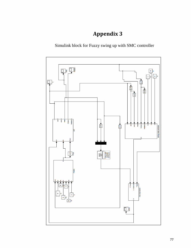
77
Appendix 3
Simulink block for Fuzzy swing up with SMC controller

78
Simulink block for Fuzzy swing up with LQR controller

79
Appendix 4
Publication
- Belal A. Elsayed, M. A. Hassan and Saad Mekhilef, Decoupled Third-
order Fuzzy Sliding Model Control For Cart-Inverted Pendulum
System, Appl. Math. Inf. Sci. 7, No. 1, 193-201 (2013) (ISI cited
publication)
- Belal A. Elsayed, M. A. Hassan and Saad Mekhilef, Fuzzy Swinging-up
with Sliding Mode Control for Third Order Cart-Inverted Pendulum
System, IEEE Transaction on Industrial Electronics.(2013) ( Submitted)