Embed Size (px)
Citation preview
University of Texas at El PasoDigitalCommons@UTEP
Open Access Theses & Dissertations
2016-01-01
G-Code Generation For Multi-Process 3D PrintingCallum Peter BaileyUniversity of Texas at El Paso, [email protected]
Follow this and additional works at: https://digitalcommons.utep.edu/open_etdPart of the Computer Engineering Commons, Electrical and Electronics Commons, and the
Mechanical Engineering Commons
This is brought to you for free and open access by DigitalCommons@UTEP. It has been accepted for inclusion in Open Access Theses & Dissertationsby an authorized administrator of DigitalCommons@UTEP. For more information, please contact [email protected].
Recommended CitationBailey, Callum Peter, "G-Code Generation For Multi-Process 3D Printing" (2016). Open Access Theses & Dissertations. 602.https://digitalcommons.utep.edu/open_etd/602
G-CODE GENERATION FOR MULTI-PROCESS
3D PRINTING
CALLUM PETER BAILEY
Master’s Program in Electrical Engineering
APPROVED:
Eric MacDonald, Ph.D., Chair
David Roberson, Ph.D.
Michael McGarry, Ph.D.
Charles Ambler, Ph.D.
Dean of the Graduate School

Copyright ©
by
Callum Peter Bailey
2016

Dedication
I dedicate this work to my parents, Peter and Jenny Bailey, whose unconditional love and
support have given me the self-confidence and self-belief to take on the world; and to my wife,
Heather, whose love has taken me on this American adventure.

G-CODE GENERATION FOR MULTI-PROCESS
3D PRINTING
by
CALLUM PETER BAILEY, MChem
THESIS
Presented to the Faculty of the Graduate School of
The University of Texas at El Paso
in Partial Fulfillment
of the Requirements
for the Degree of
MASTER OF SCIENCE
Department of Electrical & Computer Engineering
THE UNIVERSITY OF TEXAS AT EL PASO
December 2016

v
Acknowledgements
I would like to extend my acknowledgements to everyone who has contributed to this
project and who has helped me during my time in El Paso. To Dr. Eric MacDonald for inviting
me to work in his brilliant 3D printing group, with its wonderful people. To David Espalin for
his conscientious support and remarkable ability to balance student needs and objectives with the
objectives of the W.M. Keck Center for 3D Innovation. To Dr. Ryan Wicker and UTEP for
creating such a fantastic facility. To America Makes for providing funding for this work. To Dr.
David Roberson and Dr. Michael McGarry for taking the time to review this work in such a short
time frame!
To Efrain Aguilera, for being a good friend and for his outstanding contributions to both
this project and to the culinary art of discada. To Jorge Ramierez, and Alfonso Fernandez for
their work on the modified Lulzbot. To Jose Motta for his work on the Lulzbot, for helping to
print the many test jobs included in this thesis, and for sharing with me his love of menudo. To
Jake Lasley and Mike Licerio for their contributions to the GUI and other areas of the Python
program.
To Donna, Issac, Jaime, Kelly, Alex, Matt, Luis Jr. and Luis Jimenez in the MacDonald
group for the happy memories; and to Luis Bañuelos and Antonio Zúñiga for always getting me
home safely from Juárez.
vi
Abstract
Since the inception of stereolithography in the 1980s, interest in 3D printing has
exploded, with desktop 3D printers now commercially accessible to the general public. In recent
years, next-generation multifunctional technologies have been developed, which combine 3D
printing with other technologies such as wire embedding, foil embedding, CNC machining, and
robotic component placement, enabling complex parts to be made on a single multifunctional
machine.
However, the complexity of these integrated processes exceeds the capabilities of
established design tools. To this end, this thesis aims to develop a multi-functional design
solution that can automatically generate final control code for next-generation multifunctional
machines, where all design specifications are defined from within a single software package.
Specifically, we take on the task of automating a Lulzbot desktop 3D printer, which has
been modified to utilize a custom-designed wire-embedding tool as a secondary extruder. While
the algorithms presented herein have been tailored to the needs of this custom printer, the
modular nature of the solution will facilitate expansion to include other multifunctional printers,
including the planned low-cost multi3D
multifunctional printer, currently under construction at
the W.M. Keck Center for 3D Innovation at The University of Texas at El Paso.
vii
Table of Contents
Dedication ...................................................................................................................................... iii
Acknowledgements ..........................................................................................................................v
Abstract .......................................................................................................................................... vi
Table of Contents .......................................................................................................................... vii
List of Tables ................................................................................................................................. ix
List of Figures ..................................................................................................................................x
Chapter 1: Introduction ....................................................................................................................1
Fused Deposition Modeling ....................................................................................................1
3D Design and Slicing ............................................................................................................2
Multiprocess 3D Printing ........................................................................................................4
Chapter 2: Literature Review ...........................................................................................................6
Multiprocess 3D Printing of Electronics.................................................................................6
Software ................................................................................................................................10
Chapter 3: Design specifications ...................................................................................................16
Software objectives: A multi-process design and slicing methodology ...............................16
Features of the Lulzbot wire-embedding printer ..................................................................18
Foundation layer generation .................................................................................................31
Chapter 4: A method for generating multifunctional G-code ........................................................33
Introduction ...........................................................................................................................33
The Python G-code Post-processor .......................................................................................38
Summary ...............................................................................................................................67
Chapter 5: Results and Characterization ........................................................................................68
Custom Printing Parameters .................................................................................................68
Testing...................................................................................................................................70
Z Calibration .........................................................................................................................72
XY Calibration ......................................................................................................................74
FeatureDemo .........................................................................................................................76

viii
SquareCoil.............................................................................................................................78
IncreasingAngles...................................................................................................................80
Coil 84
Solenoid ................................................................................................................................86
Chapter 6: Discussion ....................................................................................................................89
Evaluation of print functions ................................................................................................89
Proposed Features and Future Work .....................................................................................91
References ......................................................................................................................................93
Appendix A: Software user procedure ...........................................................................................95
Appendix B: CreateSkin.py ...........................................................................................................99
Vita .............................................................................................................................................110

ix
List of Tables
Table 2.1 Comparison of resistivity for select conductors [20] [21] .............................................. 7 Table 3.1 Additional G-code commands utilized by the Lulzbot wire-embedding tool .............. 20 Table 5.1 Parameters used to generate the most successful execution of each print job. ............. 71 Table 5.2 Z calibration job results (G-code generation & print process). Each print function is
assessed for whether the algorithm succeeded (✓) or failed (✗) to generate G-code, and whether
the print process succeeded (✓), failed (✗), considered a partial success (½), or was not
attempted (–). N/A indicates the print function was not utilized. ................................................. 73 Table 5.3 XY calibration job results (G-code generation & print process). ................................. 75 Table 5.4 FeatureDemo job results (G-code generation & print process). ................................... 77 Table 5.5 SquareCoil job results (G-code generation & print process). ....................................... 79
Table 5.6 Test (G-code generation & print process). .................................................................... 83 Table 5.7 Coil job results (G-code generation & print process). .................................................. 85
Table 5.8 Solenoid job results (G-code generation & print process). ........................................... 87 Table 6.1 Evaluation of print functions on a variety of jobs: each print function is assessed for
whether the algorithm succeeded (✓) or failed (✗) to generate G-code, and whether the print
process succeeded (✓), failed (✗), considered a partial success (½), or was not attempted (–).
N/A indicates the print function was not utilized. ........................................................................ 89
x
List of Figures
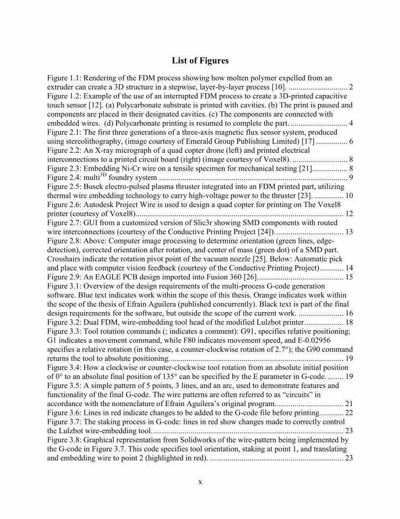
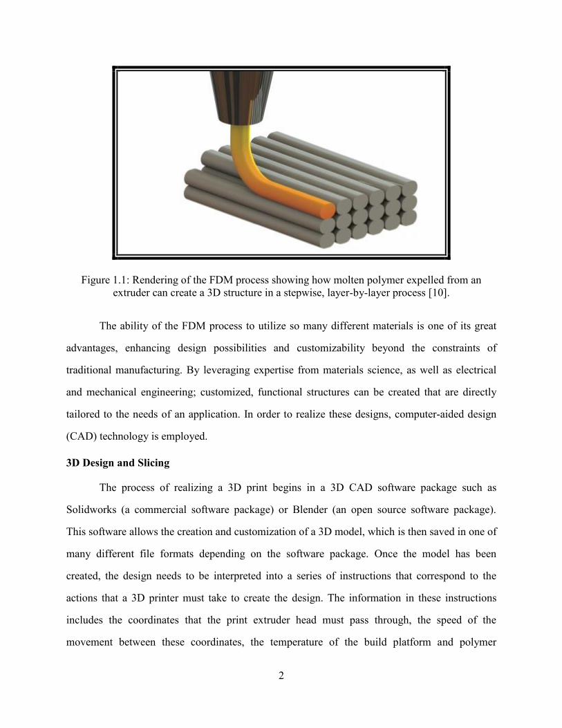
Figure 1.1: Rendering of the FDM process showing how molten polymer expelled from an
extruder can create a 3D structure in a stepwise, layer-by-layer process [10]. .............................. 2 Figure 1.2: Example of the use of an interrupted FDM process to create a 3D-printed capacitive
touch sensor [12]. (a) Polycarbonate substrate is printed with cavities. (b) The print is paused and
components are placed in their designated cavities. (c) The components are connected with
embedded wires. (d) Polycarbonate printing is resumed to complete the part. ............................. 4 Figure 2.1: The first three generations of a three-axis magnetic flux sensor system, produced
using stereolithography, (image courtesy of Emerald Group Publishing Limited) [17] ................ 6 Figure 2.2: An X-ray micrograph of a quad copter drone (left) and printed electrical
interconnections to a printed circuit board (right) (image courtesy of Voxel8). ............................ 8
Figure 2.3: Embedding Ni-Cr wire on a tensile specimen for mechanical testing [21]. ................. 8 Figure 2.4: multi
3D foundry system ................................................................................................ 9
Figure 2.5: Busek electro-pulsed plasma thruster integrated into an FDM printed part, utilizing
thermal wire embedding technology to carry high-voltage power to the thruster [23]. ............... 10
Figure 2.6: Autodesk Project Wire is used to design a quad copter for printing on The Voxel8
printer (courtesy of Voxel8).......................................................................................................... 12
Figure 2.7: GUI from a customized version of Slic3r showing SMD components with routed
wire interconnections (courtesy of the Conductive Printing Project [24]). .................................. 13 Figure 2.8: Above: Computer image processing to determine orientation (green lines, edge-
detection), corrected orientation after rotation, and center of mass (green dot) of a SMD part.
Crosshairs indicate the rotation pivot point of the vacuum nozzle [25]. Below: Automatic pick
and place with computer vision feedback (courtesy of the Conductive Printing Project) ............ 14 Figure 2.9: An EAGLE PCB design imported into Fusion 360 [26]. ........................................... 15
Figure 3.1: Overview of the design requirements of the multi-process G-code generation
software. Blue text indicates work within the scope of this thesis. Orange indicates work within
the scope of the thesis of Efrain Aguilera (published concurrently). Black text is part of the final
design requirements for the software, but outside the scope of the current work. ....................... 16 Figure 3.2: Dual FDM, wire-embedding tool head of the modified Lulzbot printer .................... 18
Figure 3.3: Tool rotation commands (; indicates a comment): G91, specifies relative positioning;
G1 indicates a movement command, while F80 indicates movement speed, and E-0.02956
specifies a relative rotation (in this case, a counter-clockwise rotation of 2.7°); the G90 command
returns the tool to absolute positioning. ........................................................................................ 19 Figure 3.4: How a clockwise or counter-clockwise tool rotation from an absolute initial position
of 0° to an absolute final position of 135° can be specified by the E parameter in G-code. ........ 19
Figure 3.5: A simple pattern of 5 points, 3 lines, and an arc, used to demonstrate features and
functionality of the final G-code. The wire patterns are often referred to as “circuits” in
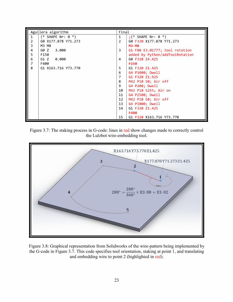
accordance with the nomenclature of Efrain Aguilera’s original program. .................................. 21 Figure 3.6: Lines in red indicate changes to be added to the G-code file before printing. ........... 22 Figure 3.7: The staking process in G-code: lines in red show changes made to correctly control
the Lulzbot wire-embedding tool. ................................................................................................. 23 Figure 3.8: Graphical representation from Solidworks of the wire-pattern being implemented by
the G-code in Figure 3.7. This code specifies tool orientation, staking at point 1, and translating
and embedding wire to point 2 (highlighted in red). .................................................................... 23

xi
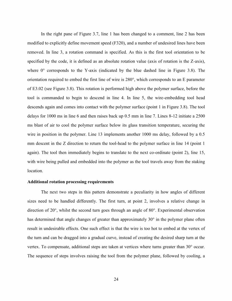
Figure 3.9: Small and large rotations implemented in G-code: lines in red show changes made to
correctly control the Lulzbot wire-embedding tool. ..................................................................... 25 Figure 3.10: Graphical representation of the small (point 2) and large (points 3 and 4) rotations
required by the wire-pattern. Turns at points 2 and 3 and the translational lines in red are
generated by the G-code in Figure 3.9. ......................................................................................... 26 Figure 3.11: G2 and G3 arc to G1 line interpolation in G-code: lines in red show changes made
to correctly control the Lulzbot wire-embedding tool. Short lines and rotations between lines 48
and 165, which have syntax similar to lines 45-48, have been omitted for brevity. ..................... 27 Figure 3.12: Graphical representation of the arc (between points 4 and 5) implemented by the G-
code in Figure 3.11. The relation between the I and J components of the G3 command and the
origin of the arc is clearly visible. ................................................................................................. 28 Figure 3.13: The cutting process in G-code: lines in red show changes made to correctly control
the Lulzbot wire-embedding tool. A line by-line description is given below. ............................. 29
Figure 3.14: Graphical representation from Solidworks of the wire-pattern being implemented by
the G-code in Figure 3.13. The tool is already at point 5, so the only remaining step is to cut the
wire. .............................................................................................................................................. 30 Figure 3.15: Solid polymer skin pattern necessary to provide a suitable foundation for wire-
embedding. .................................................................................................................................... 31 Figure 3.16: Example of replacing a sparse fill section with a solid skin in G-code.................... 32 Figure 4.1: Workflow for generating multi-functional G-code (approach developed by Efrain
Aguilera). Orange indicates process steps created by Efrain Aguilera; Blue steps indicate work
within the scope of this thesis. ...................................................................................................... 34
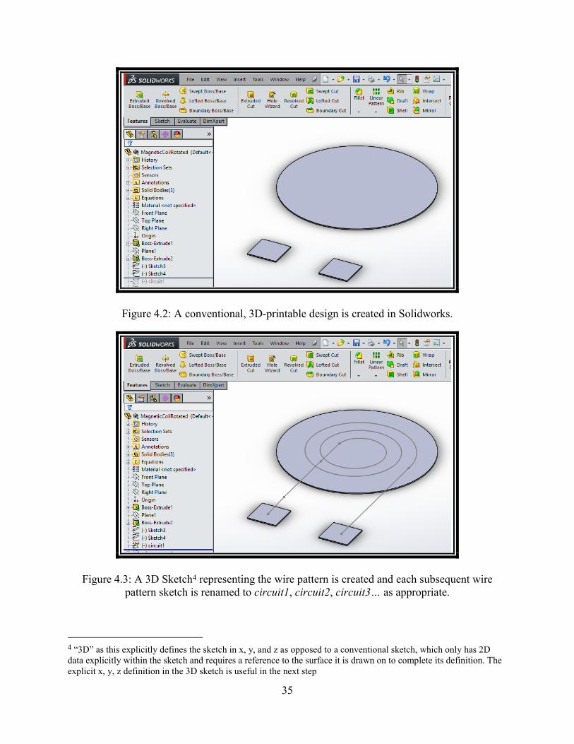
Figure 4.2: A conventional, 3D-printable design is created in Solidworks. ................................. 35 Figure 4.3: A 3D Sketch representing the wire pattern is created and each subsequent wire
pattern sketch is renamed to circuit1, circuit2, circuit3… as appropriate. ................................... 35
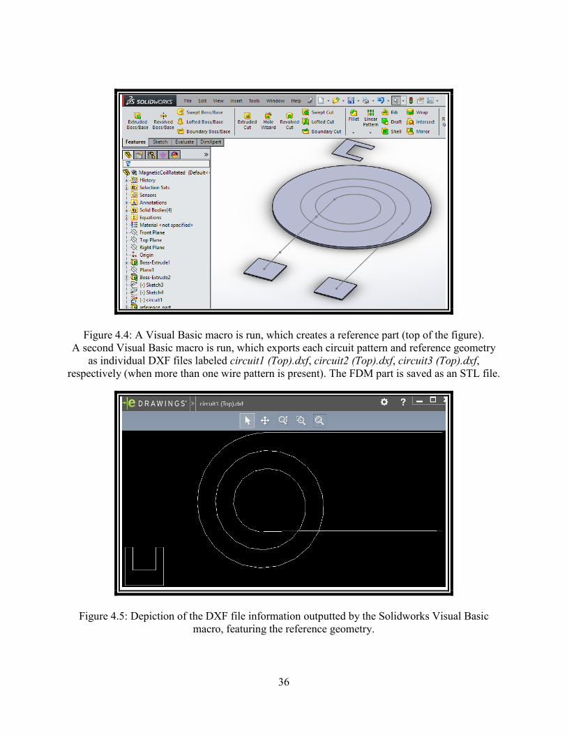
Figure 4.4: A Visual Basic macro is run, which creates a reference part (top of the figure). A
second Visual Basic macro is run, which exports each circuit pattern and reference geometry as
individual DXF files labeled circuit1 (Top).dxf, circuit2 (Top).dxf, circuit3 (Top).dxf,
respectively (when more than one wire pattern is present). The FDM part is saved as an STL file.
....................................................................................................................................................... 36 Figure 4.5: Depiction of the DXF file information outputted by the Solidworks Visual Basic
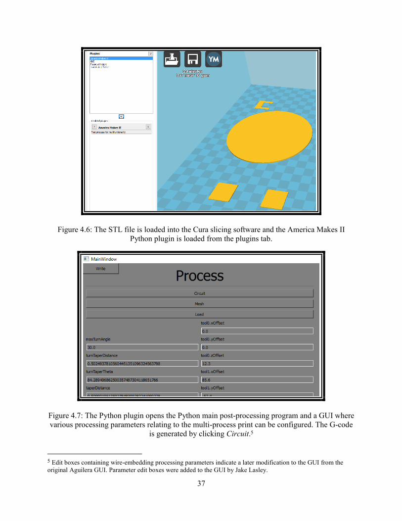
macro, featuring the reference geometry. ..................................................................................... 36 Figure 4.6: The STL file is loaded into the Cura slicing software and the America Makes II
Python plugin is loaded from the plugins tab. .............................................................................. 37 Figure 4.7: The Python plugin opens the Python main post-processing program and a GUI where
various processing parameters relating to the multi-process print can be configured. The G-code
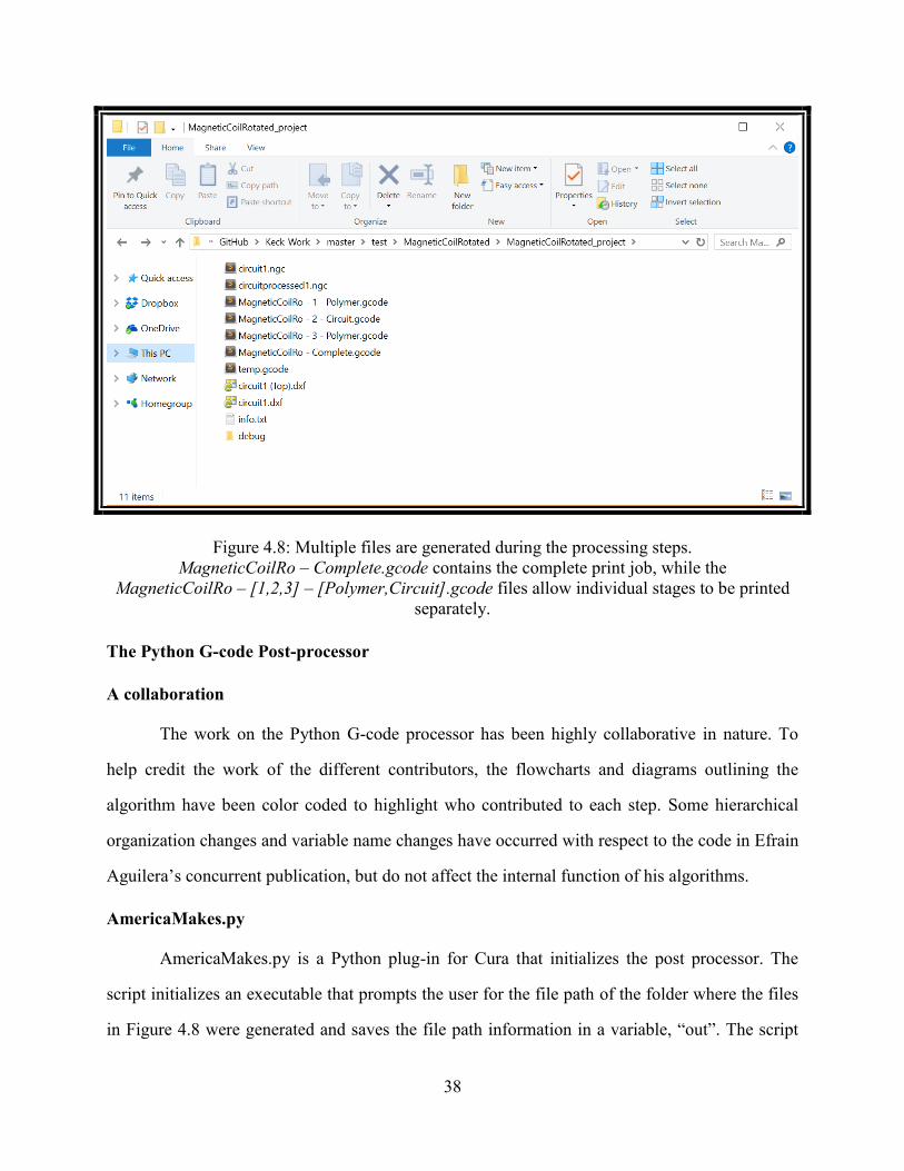
is generated by clicking Circuit. ................................................................................................... 37 Figure 4.8: Multiple files are generated during the processing steps. MagneticCoilRo –
Complete.gcode contains the complete print job, while the MagneticCoilRo – [1,2,3] –
[Polymer,Circuit].gcode files allow individual stages to be printed separately. .......................... 38
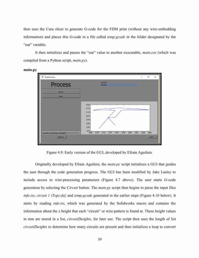
Figure 4.9: Early version of the GUI, developed by Efrain Aguilera. .......................................... 39 Figure 4.10: Overview (1 of 3) of the steps of the addCircuit function of the main.py program.
Orange indicates process steps created by Efrain Aguilera; Blue indicates process steps
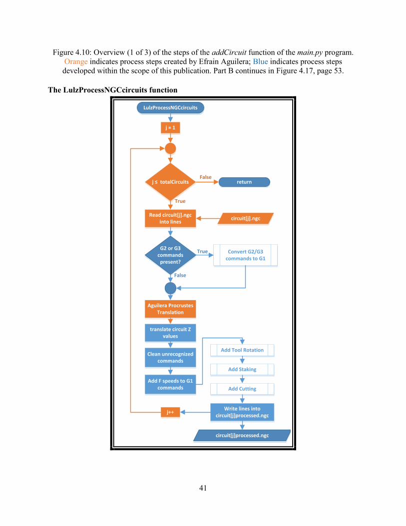
developed within the scope of this publication. Part B continues in Figure 4.17, page 53. ......... 41 Figure 4.11: Overview of the LulzProcessNGCcircuits algorithm which generates wire-extruding
G-code for the modified Lulzbot. Orange indicate steps generated by Efrain Aguilera. Blue steps

xii
relate to this publication. In this algorithm, the input is the circuit[j].ngc file generated by
DXF2GCODE.exe; the output is the circuit[j]processed.ngc file which contains correctly-
formatted G-code for each circuit pattern. .................................................................................... 42 Figure 4.12: G2 conversion algorithm. All steps in this function relate to this publication. ........ 43
Figure 4.13: Algorithm for creating a list of straight line G1 commands for a given G2 command
....................................................................................................................................................... 44 Figure 4.14: Part of the addToolRotation function, used to generate correct tool orientation. .... 47 Figure 4.15: The addStaking function. ......................................................................................... 49 Figure 4.16: The addCutting function. .......................................................................................... 50
Figure 4.17: Overview (2 of 3) of the main.py addCircuit function. Orange indicates process
steps created by Efrain Aguilera; Blue indicates process steps within the scope of this
publication. Continued from Figure 4.10, page 41. ...................................................................... 53 Figure 4.18: Overview (1 of 2) of the CreateSkin function. All process steps illustrated are within
the scope of this publication. Continued in Figure 4.19. .............................................................. 54 Figure 4.19: Overview (2 of 2) of the CreateSkin function. ......................................................... 56
Figure 4.20: QuantizeY function. ................................................................................................. 57 Figure 4.21: Overview (3 of 3) of the main.py addCircuit function. All process steps illustrated
are within the scope of this publication. Continued from Figure 4.17, page 53. .......................... 58 Figure 4.22: transformPolymerZ(lines, zOffset) modifies all polymer lines by the zOffset. ....... 59 Figure 4.23: checkBoundaryLimits(cLines, BoundaryMin, BoundaryMax) ensures generated G-
code remains within the build area. .............................................................................................. 60 Figure 4.24: FileSlicer(cLines, filePath) generates the final G-code files with appropriate headers
and footers. .................................................................................................................................... 61 Figure 4.25: sliceLines(lines) function within fileSlicer function separates the polymer and
circuit sections. ............................................................................................................................. 62
Figure 4.26: generateIndividualFiles function within fileSlicer function separates the polymer
and circuit sections. ....................................................................................................................... 64 Figure 4.27: The generateFinalOutputFile function within fileSlicer function combines all G-
code into a single print job. ........................................................................................................... 66
Figure 4.28: Summary of G-code post-processing requirements that have been addressed. ....... 67 Figure 5.1: Parameters available in the GUI. ................................................................................ 68
Figure 5.2: A fast and simple Z calibration job to determine wire-embedding efficacy and to
allow for a quick iterative adjustment of tool1.zOffet. ................................................................. 72
Figure 5.3: Top: Z Calibration job with 100% infill immediately after wire embedding; Middle:
Z Calibration job with 100% infill after the top layers have been printed. Bottom: Z Calibration
job with 20% infill, utilizing CreateSkin to create 100% fill below the wire and sparse (20% fill)
above the wire. The poor coverage of the top layer is a print artefact, unrelated to CreateSkin. . 73 Figure 5.4: XY calibration job ...................................................................................................... 74
Figure 5.5: Unfortunately, the XY calibration job did not live up to expectations. ..................... 75 Figure 5.6: FeatureDemo design ................................................................................................... 76
Figure 5.7: FeatureDemo print result ............................................................................................ 77 Figure 5.8: CreateSkin in FeatureDemo ....................................................................................... 78 Figure 5.9: SquareCoil design....................................................................................................... 78 Figure 5.10: SquareCoil print result.............................................................................................. 79 Figure 5.11: IncreasingAngles design........................................................................................... 80 Figure 5.12: IncreasingAngles print result.................................................................................... 81

xiii
Figure 5.13: Using the DXF2GCODE.exe GUI to manually reverse staking and print
directionality. ................................................................................................................................ 82 Figure 5.14: Generated G-code of wire tool-path visualized using web-based toolpath simulator
(colors inverted) [29].The upper image features the disfavored original direction; the lower
image features the favored reversed direction. It is preferable to have a straighter initial section
(lower) to improve initial staking and wire-embedding. Light blue shows G0 commands. Black
shows G1 commands. Large turns can be visualized by the small Z rise causing a “bump” for
angles greater than maxTurnAngle (30°) ...................................................................................... 83 Figure 5.15: Coil design. ............................................................................................................... 84
Figure 5.16: Coil job immediately after wire-embedding layer (left) and after the top layers have
been printed (right) ....................................................................................................................... 85 Figure 5.17: Solenoid design. ....................................................................................................... 86 Figure 5.18: Solenoid print job parts 1-7, alternating between Polymer (odd numbers) and Circuit
pattern (even numbers). Part 4 circuit pattern is omitted as it completely failed to stake or embed.
....................................................................................................................................................... 87
1
Chapter 1: Introduction
The advent of modern 3D printing is widely attributed to Charles Hull and his invention
of the stereolithography (SLA) rapid prototyping process, over 30 years ago. This process uses
photocurable resins and light to create custom three-dimensional solid bodies [1]. Since then,
many different additive manufacturing processes have been developed: fused deposition
modeling (FDM), Polyjet, laminated object manufacturing (LOM), Prometal, selective laser
sintering (SLS), laminated engineered net shaping (LENS), and electron beam melting (EBM)
[2]. While initially envisioned to create models, applications of these technologies have since
diversified widely: from biomedical prostheses, customized pharmaceuticals, aircraft
components, tooling, mass-customized parts, and artwork [3–8].
Fused Deposition Modeling
Patented by Stratasys founder Scott Crump in 1989 [9], The FDM process involves the
deposition of a thin strand (typically 0.25 mm diameter) of molten thermoplastic resin to build a
three-dimensional structure in a stepwise, layer-by-layer manner. The technology can be used
with a wide range of materials, with acrylonitrile butadiene styrene (ABS) and polylactic acid
(PLA) being the most ubiquitous in consumer 3D printers. Widely-used materials in industrial-
grade 3D printers include polycarbonate (PC) and Nylon, as well as proprietary performance
polymers such as ULTEM™, a polyetherimide resin manufactured by Sabic (Pittsfield, MA).
2
Figure 1.1: Rendering of the FDM process showing how molten polymer expelled from an
extruder can create a 3D structure in a stepwise, layer-by-layer process [10].
The ability of the FDM process to utilize so many different materials is one of its great
advantages, enhancing design possibilities and customizability beyond the constraints of
traditional manufacturing. By leveraging expertise from materials science, as well as electrical
and mechanical engineering; customized, functional structures can be created that are directly
tailored to the needs of an application. In order to realize these designs, computer-aided design
(CAD) technology is employed.
3D Design and Slicing
The process of realizing a 3D print begins in a 3D CAD software package such as
Solidworks (a commercial software package) or Blender (an open source software package).
This software allows the creation and customization of a 3D model, which is then saved in one of
many different file formats depending on the software package. Once the model has been
created, the design needs to be interpreted into a series of instructions that correspond to the
actions that a 3D printer must take to create the design. The information in these instructions
includes the coordinates that the print extruder head must pass through, the speed of the
movement between these coordinates, the temperature of the build platform and polymer
3
extruder head, whether the print extruder head should be extruding polymer, the rate of polymer
extrusion, as well as any other miscellaneous input or output (I/O) control associated with the
printer. If the printer has more than one extruder, which extruder to use and its temperature must
also be specified. The most popular open-source instruction language used to convey this
information is G-code, although manufacturers have also developed their own proprietary
solutions. The software used to generate the G-code is known as a slicer.
Just as there are many CAD tools available for generating 3D parts, there are many
slicers available for converting these parts into printable G-code: including Stratasys Insight
(commercial, license-required), MakerBot Desktop (commercial, free to use), Cura (open
source), and Slic3r (open source). Insight and MakerBot output proprietary file-formats useable
by their print hardware, while Cura and Slic3r output standard G-code files. In common, they all
require the 3D model to be presented in a standardized format that the slicer can read. The most
popular format is the stereolithography (STL) file format developed by 3D Systems [11]. While
originally developed for 3D Systems’ stereolithography process, the STL file format is used
widely in a variety of additive manufacturing technologies, including FDM. This file format
defines the surface geometry of a 3D part through a series of tessellated triangles. These triangles
can be parsed by slicing software to convert them into layers of printable G-code coordinates.
However, as this file format only stores information on geometry and not material type, it
presents severe limitations when trying to utilize it to design and slice multi-material and multi-
process parts. An additional limitation is that all STL parts must have volume or area, whereas to
provide instructions for a wire-embedding tool, one may only require a line that has no volume
or area.
Another capability of the FDM process is that it can be readily interrupted. This allows a
print job to be paused, so that external electronic or mechanical components can be inserted into
predesigned cavities, and then resumed to encapsulate the components in polymer. By this
4
method, customized electromechanical devices containing springs, motors, antennas,
microprocessors, as well as other circuit components can be created. This capacity of 3D printing
to accomplish novel electromechanical designs has sparked interest in multiprocess 3D printing.
Multiprocess 3D Printing
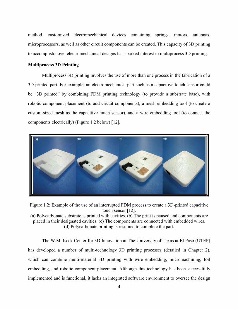
Multiprocess 3D printing involves the use of more than one process in the fabrication of a
3D-printed part. For example, an electromechanical part such as a capacitive touch sensor could
be “3D printed” by combining FDM printing technology (to provide a substrate base), with
robotic component placement (to add circuit components), a mesh embedding tool (to create a
custom-sized mesh as the capacitive touch sensor), and a wire embedding tool (to connect the
components electrically) (Figure 1.2 below) [12].
Figure 1.2: Example of the use of an interrupted FDM process to create a 3D-printed capacitive
touch sensor [12].
(a) Polycarbonate substrate is printed with cavities. (b) The print is paused and components are
placed in their designated cavities. (c) The components are connected with embedded wires.
(d) Polycarbonate printing is resumed to complete the part.
The W.M. Keck Center for 3D Innovation at The University of Texas at El Paso (UTEP)
has developed a number of multi-technology 3D printing processes (detailed in Chapter 2),
which can combine multi-material 3D printing with wire embedding, micromachining, foil
embedding, and robotic component placement. Although this technology has been successfully
implemented and is functional, it lacks an integrated software environment to oversee the design

5
process over the differing technologies. This requires the human operator to calculate at what
layer a pause should be manually added to a print, and what kind of coordinate offsets need to be
introduced to integrate the various design tools.
6
Chapter 2: Literature Review
Multiprocess 3D Printing of Electronics
Conductive Inks
The in situ fabrication of complex electromechanical devices via 3D-printing has been
occurring for over 15 years [13]. Some of the earliest 3D-printed complex devices were
fabricated by pausing an SLA print process and inserting an external electronic component into a
specially-designed cavity in the print [13]. This process was augmented by the introduction of
conductive inks to the SLA process by Palmer et al. [14] and Medina et al. [15], [16], allowing
the in situ creation of simple circuits during the additive manufacturing process.
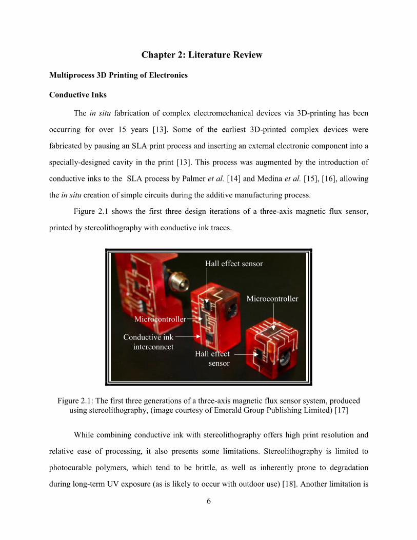
Figure 2.1 shows the first three design iterations of a three-axis magnetic flux sensor,
printed by stereolithography with conductive ink traces.
Figure 2.1: The first three generations of a three-axis magnetic flux sensor system, produced
using stereolithography, (image courtesy of Emerald Group Publishing Limited) [17]
While combining conductive ink with stereolithography offers high print resolution and
relative ease of processing, it also presents some limitations. Stereolithography is limited to
photocurable polymers, which tend to be brittle, as well as inherently prone to degradation
during long-term UV exposure (as is likely to occur with outdoor use) [18]. Another limitation is
Hall effect sensor
Conductive ink
interconnect
Microcontroller
Hall effect
sensor
Microcontroller
7
the low conductivity of conductive inks, which tend to be two orders of magnitude less
conductive than a traditional bulk metal conductor, such as copper [19]. This limits the use of
conductive inks in electronics to applications with low power requirements.
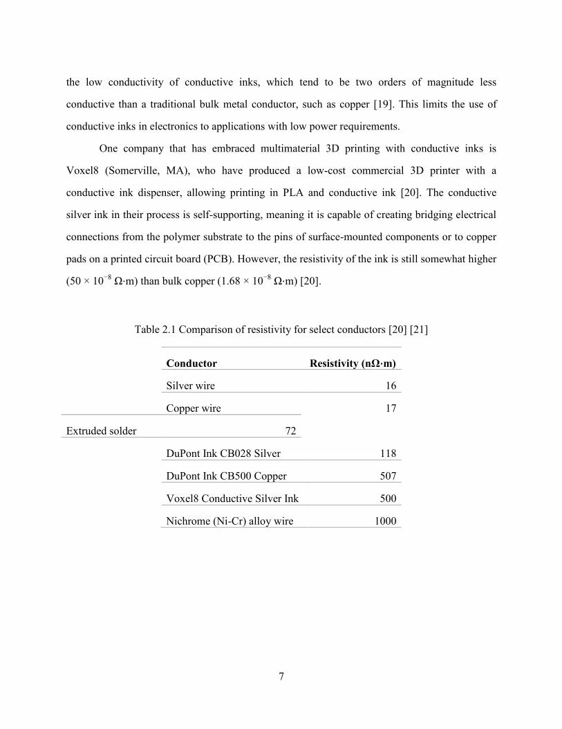
One company that has embraced multimaterial 3D printing with conductive inks is
Voxel8 (Somerville, MA), who have produced a low-cost commercial 3D printer with a
conductive ink dispenser, allowing printing in PLA and conductive ink [20]. The conductive
silver ink in their process is self-supporting, meaning it is capable of creating bridging electrical
connections from the polymer substrate to the pins of surface-mounted components or to copper
pads on a printed circuit board (PCB). However, the resistivity of the ink is still somewhat higher
(50 × 10−8
Ω⋅m) than bulk copper (1.68 × 10⁻⁸
Ω⋅m) [20].
Table 2.1 Comparison of resistivity for select conductors [20] [21]
Conductor Resistivity (nΩ⋅m)
Silver wire 16
Copper wire 17
Extruded solder 72
DuPont Ink CB028 Silver 118
DuPont Ink CB500 Copper 507
Voxel8 Conductive Silver Ink 500
Nichrome (Ni-Cr) alloy wire 1000
8
Figure 2.2: An X-ray micrograph of a quad copter drone (left) and printed electrical
interconnections to a printed circuit board (right) (image courtesy of Voxel8).
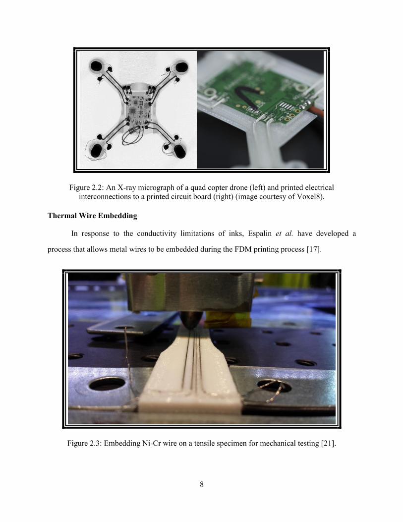
Thermal Wire Embedding
In response to the conductivity limitations of inks, Espalin et al. have developed a
process that allows metal wires to be embedded during the FDM printing process [17].
Figure 2.3: Embedding Ni-Cr wire on a tensile specimen for mechanical testing [21].
9
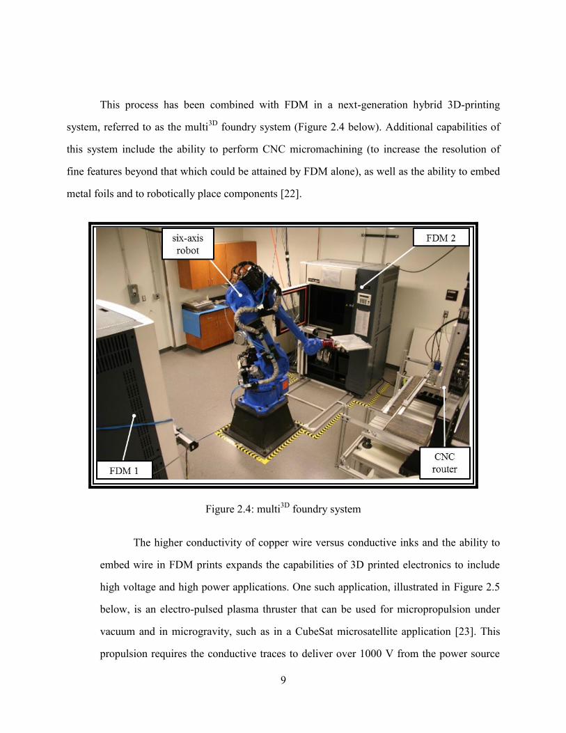
This process has been combined with FDM in a next-generation hybrid 3D-printing
system, referred to as the multi3D
foundry system (Figure 2.4 below). Additional capabilities of
this system include the ability to perform CNC micromachining (to increase the resolution of
fine features beyond that which could be attained by FDM alone), as well as the ability to embed
metal foils and to robotically place components [22].
Figure 2.4: multi3D
foundry system
The higher conductivity of copper wire versus conductive inks and the ability to
embed wire in FDM prints expands the capabilities of 3D printed electronics to include
high voltage and high power applications. One such application, illustrated in Figure 2.5
below, is an electro-pulsed plasma thruster that can be used for micropropulsion under
vacuum and in microgravity, such as in a CubeSat microsatellite application [23]. This
propulsion requires the conductive traces to deliver over 1000 V from the power source
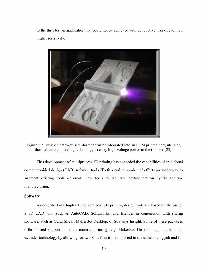
10
to the thruster: an application that could not be achieved with conductive inks due to their
higher resistivity.
Figure 2.5: Busek electro-pulsed plasma thruster integrated into an FDM printed part, utilizing
thermal wire embedding technology to carry high-voltage power to the thruster [23].
This development of multiprocess 3D printing has exceeded the capabilities of traditional
computer-aided design (CAD) software tools. To this end, a number of efforts are underway to
augment existing tools or create new tools to facilitate next-generation hybrid additive
manufacturing.
Software
As described in Chapter 1, conventional 3D printing design tools are based on the use of
a 3D CAD tool, such as AutoCAD, Solidworks, and Blender in conjunction with slicing
software, such as Cura, Slic3r, MakerBot Desktop, or Stratasys Insight. Some of these packages
offer limited support for multi-material printing: e.g. MakerBot Desktop supports its dual-
extruder technology by allowing for two STL files to be imported to the same slicing job and for
11
each solid body to be designated to be printed with a specified extruder. However, this solution
still presents some design limitations and complexity. It would be advantageous if the material
requirements could be designated during the CAD design stage, with the information preserved
through the slicing process and into the final G-code. This is not easy to do with the conventional
STL file format, as this file contains only geometric information (in the form of tessellated
triangles that define the surface geometry). More advanced file formats have been developed,
including the open standard AMF (additive manufacturing file) file format, as well as the 3MF
Consortium’s 3MF (3D manufacturing format). The AMF format is an ASTM standard, while
the 3MF format is supported by some of the largest industry leaders in 3D printing: 3D Systems,
Stratasys, Shapeways, GE, HP, Dassault Systèmes, Ultimaker, and Microsoft. Both AMF and
3MF are XML-based (extensible markup language) file formats that provide multi-material
support, as well as allowing for the incorporation of metadata. In addition, 3MF provides support
for subtractive manufacturing processes, such as CNC machining, and is designed around the
principle of extendibility to facilitate the addition of new functionality in the future.
Unfortunately, the slicing software has not kept pace with these new developments, and while
slicing software may be capable of reading vertex information in these new file formats, it cannot
utilize the additional information to generate multi-functional G-code for next-generation hybrid
3D printers.
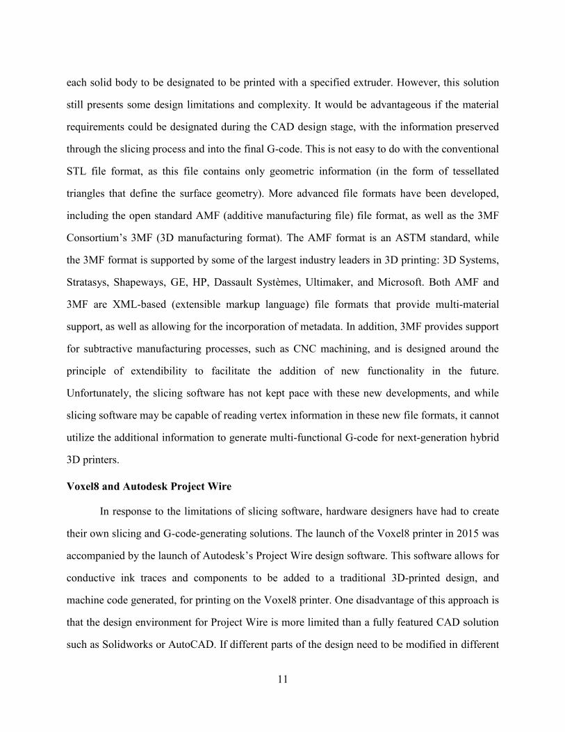
Voxel8 and Autodesk Project Wire
In response to the limitations of slicing software, hardware designers have had to create
their own slicing and G-code-generating solutions. The launch of the Voxel8 printer in 2015 was
accompanied by the launch of Autodesk’s Project Wire design software. This software allows for
conductive ink traces and components to be added to a traditional 3D-printed design, and
machine code generated, for printing on the Voxel8 printer. One disadvantage of this approach is
that the design environment for Project Wire is more limited than a fully featured CAD solution
such as Solidworks or AutoCAD. If different parts of the design need to be modified in different
12
design tools, this may present difficulties with synchronizing design changes during an iterative
design-refinement process. Project Wire’s library of integrated circuits (ICs) is also somewhat
limited, requiring additional work on the part of the end user to develop their own library of
commonly used ICs.
Figure 2.6: Autodesk Project Wire is used to design a quad copter for printing on The Voxel8
printer (courtesy of Voxel8).
User-modified Slic3r
Another approach is to augment existing slicing software. Wasserfall has created an
electronics extension for the open-source slicing tool, Slic3r. This modified tool allows for
surface-mounted components and wires to be added to an existing design and visualized from
within the Slic3r graphical user interface (GUI) [24]. When components or wires are placed, the
software automatically adjusts the polymer slicing to provide appropriate cavities and a support
layer underneath the components. Figure 2.8, below, shows how a solid layer in yellow is placed
underneath wires and components, with a less dense infill layer in pink to improve print speed
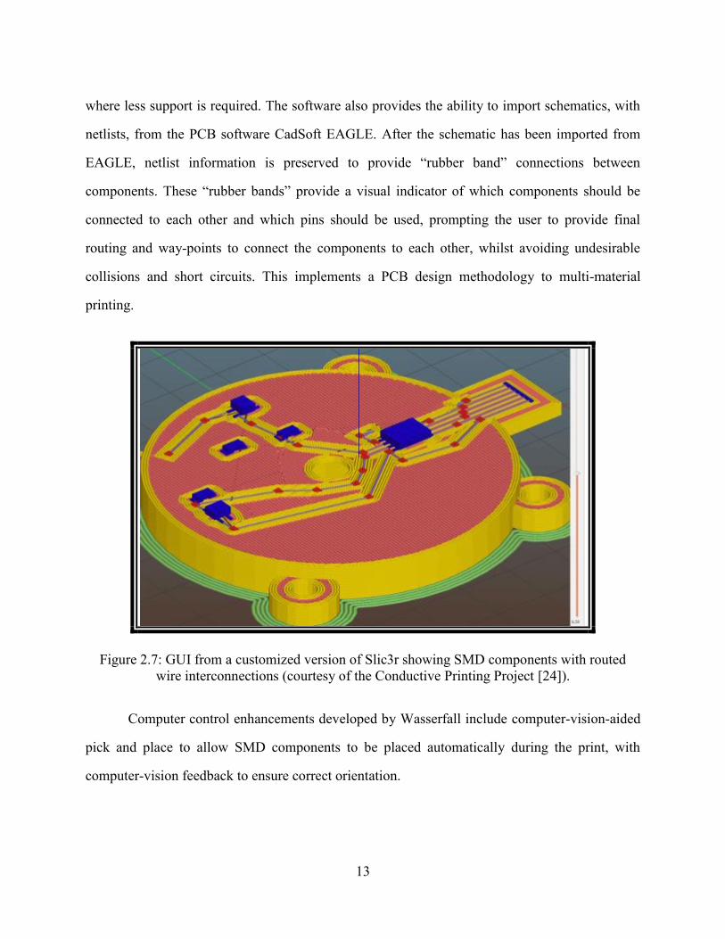
13
where less support is required. The software also provides the ability to import schematics, with
netlists, from the PCB software CadSoft EAGLE. After the schematic has been imported from
EAGLE, netlist information is preserved to provide “rubber band” connections between
components. These “rubber bands” provide a visual indicator of which components should be
connected to each other and which pins should be used, prompting the user to provide final
routing and way-points to connect the components to each other, whilst avoiding undesirable
collisions and short circuits. This implements a PCB design methodology to multi-material
printing.
Figure 2.7: GUI from a customized version of Slic3r showing SMD components with routed
wire interconnections (courtesy of the Conductive Printing Project [24]).
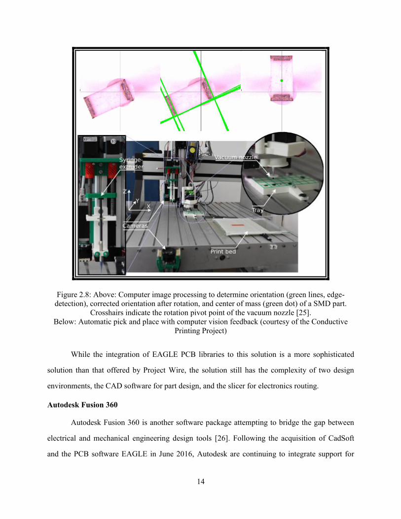
Computer control enhancements developed by Wasserfall include computer-vision-aided
pick and place to allow SMD components to be placed automatically during the print, with
computer-vision feedback to ensure correct orientation.
14
Figure 2.8: Above: Computer image processing to determine orientation (green lines, edge-
detection), corrected orientation after rotation, and center of mass (green dot) of a SMD part.
Crosshairs indicate the rotation pivot point of the vacuum nozzle [25].
Below: Automatic pick and place with computer vision feedback (courtesy of the Conductive
Printing Project)
While the integration of EAGLE PCB libraries to this solution is a more sophisticated
solution than that offered by Project Wire, the solution still has the complexity of two design
environments, the CAD software for part design, and the slicer for electronics routing.
Autodesk Fusion 360
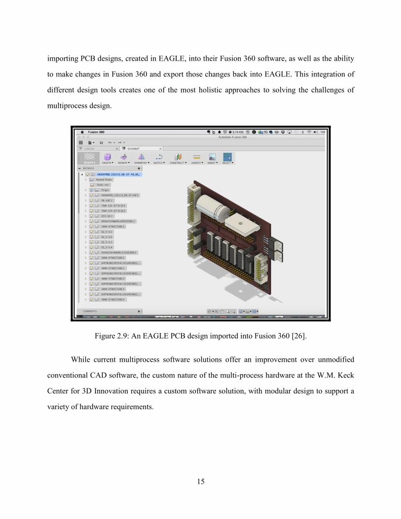
Autodesk Fusion 360 is another software package attempting to bridge the gap between
electrical and mechanical engineering design tools [26]. Following the acquisition of CadSoft
and the PCB software EAGLE in June 2016, Autodesk are continuing to integrate support for
15
importing PCB designs, created in EAGLE, into their Fusion 360 software, as well as the ability
to make changes in Fusion 360 and export those changes back into EAGLE. This integration of
different design tools creates one of the most holistic approaches to solving the challenges of
multiprocess design.
Figure 2.9: An EAGLE PCB design imported into Fusion 360 [26].
While current multiprocess software solutions offer an improvement over unmodified
conventional CAD software, the custom nature of the multi-process hardware at the W.M. Keck
Center for 3D Innovation requires a custom software solution, with modular design to support a
variety of hardware requirements.
16
Chapter 3: Design specifications
Software objectives: A multi-process design and slicing methodology
Multi-process 3D
printing software
Supported
hardware
· Lulzbot
· Low-cost multi3D
· Big Area Additive
Manufacturing (BAAM)
Supported
processes
· FDM
· Wire-embedding
· Robotic component
placement
· CNC machining
· Mesh/foil embedding
Design
requirements
· G-code output
· STL, AMF, or 3MF
support
· Interface with existing
design software
(Solidworks, Eagle)
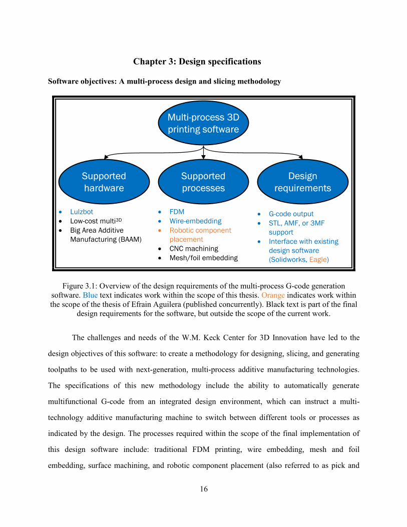
Figure 3.1: Overview of the design requirements of the multi-process G-code generation
software. Blue text indicates work within the scope of this thesis. Orange indicates work within
the scope of the thesis of Efrain Aguilera (published concurrently). Black text is part of the final
design requirements for the software, but outside the scope of the current work.
The challenges and needs of the W.M. Keck Center for 3D Innovation have led to the
design objectives of this software: to create a methodology for designing, slicing, and generating
toolpaths to be used with next-generation, multi-process additive manufacturing technologies.
The specifications of this new methodology include the ability to automatically generate
multifunctional G-code from an integrated design environment, which can instruct a multi-
technology additive manufacturing machine to switch between different tools or processes as
indicated by the design. The processes required within the scope of the final implementation of
this design software include: traditional FDM printing, wire embedding, mesh and foil
embedding, surface machining, and robotic component placement (also referred to as pick and

17
place). The mechanical-engineering challenges of these processes are reasonably well-
understood, with more comprehensive automation currently limited by the lack of a holistic CAD
software solution. Other desirable processes outside the current scope of this software solution
include the automated placement of vias, as well as automated laser-welding or soldering to
connect components. These mechanical processes require further design refinement and so are
outside the scope of the planned low-cost multi3D
printer.
Many of these objectives go beyond what could be expected to be achieved by one
person or within the timeline of a master’s thesis. As such, the scope of this thesis is restricted to
the refinement of a multi-process FDM and wire-embedding methodology on the modified
Lulzbot printer.
18
Features of the Lulzbot wire-embedding printer
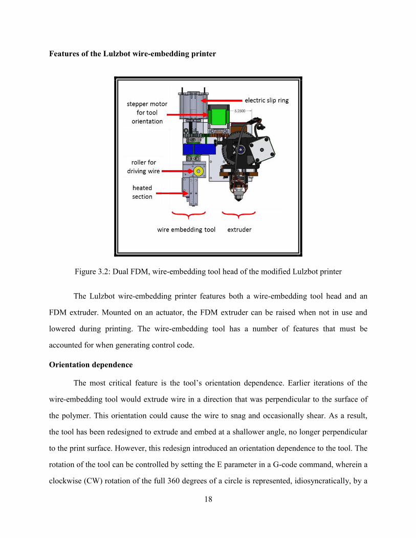
Figure 3.2: Dual FDM, wire-embedding tool head of the modified Lulzbot printer
The Lulzbot wire-embedding printer features both a wire-embedding tool head and an
FDM extruder. Mounted on an actuator, the FDM extruder can be raised when not in use and
lowered during printing. The wire-embedding tool has a number of features that must be
accounted for when generating control code.
Orientation dependence
The most critical feature is the tool’s orientation dependence. Earlier iterations of the
wire-embedding tool would extrude wire in a direction that was perpendicular to the surface of
the polymer. This orientation could cause the wire to snag and occasionally shear. As a result,
the tool has been redesigned to extrude and embed at a shallower angle, no longer perpendicular
to the print surface. However, this redesign introduced an orientation dependence to the tool. The
rotation of the tool can be controlled by setting the E parameter in a G-code command, wherein a
clockwise (CW) rotation of the full 360 degrees of a circle is represented, idiosyncratically, by a
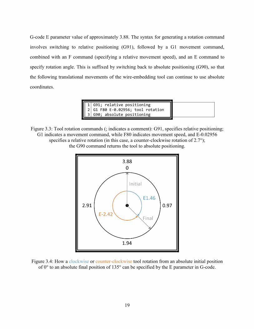
19
G-code E parameter value of approximately 3.88. The syntax for generating a rotation command
involves switching to relative positioning (G91), followed by a G1 movement command,
combined with an F command (specifying a relative movement speed), and an E command to
specify rotation angle. This is suffixed by switching back to absolute positioning (G90), so that
the following translational movements of the wire-embedding tool can continue to use absolute
coordinates.
1 2 3
G91; relative positioning G1 F80 E-0.02956; tool rotation G90; absolute positioning
Figure 3.3: Tool rotation commands (; indicates a comment): G91, specifies relative positioning;
G1 indicates a movement command, while F80 indicates movement speed, and E-0.02956
specifies a relative rotation (in this case, a counter-clockwise rotation of 2.7°);
the G90 command returns the tool to absolute positioning.
Figure 3.4: How a clockwise or counter-clockwise tool rotation from an absolute initial position
of 0° to an absolute final position of 135° can be specified by the E parameter in G-code.

20
Custom commands
In addition to the regular X, Y, Z coordinates and F speed commands. The wire-
embedding tool utilizes a number of custom and less common G-code commands, which must be
implemented in the wire-embedding G-code for the tool to function correctly.
Table 3.1 Additional G-code commands utilized by the Lulzbot wire-embedding tool
G-code command Description
M42 P14 Sx Wire Extruder Feed Motor1
(x: 0=off 255=on)
M42 P16 Sx Wire cutting tool
(x: 0=off 255=on)
M42 P18 Sx Cooling air
(x: 0=off 255=on)
M104 T1 Wire extruder temp
G4 Px Dwell (delay) for x ms
G90 Absolute G-code references
G91 Relative G-code references
T0 FDM extruder tool
T1 Wire-embedding tool
E Polymer extrusion (T0)
Tool rotation (T1)
1 This motor is not currently physically implemented on the tool.
21
Before we determine how we get there, we must first know where we’re going. I.e. what
is the nature of the post processing G-code that we are striving to generate and how does it differ
from the G-code generated by our current slicers or algorithms? By a combination of Efrain
Aguilera’s original post processing program (whose work will be referred to throughout this
thesis, and which will be published concurrently), as well as MatLab scripts, and hand-coded
changes, the mechanical engineers in the W.M. Keck Center for 3D Innovation have been able to
experimentally determine which G-code sequences should be included in the final output of the
post-processing program for optimal control of the Lulzbot printer. To illustrate these G-code
commands and their purpose, a sample design has been chosen that will highlight design
specifications of the final G-code.
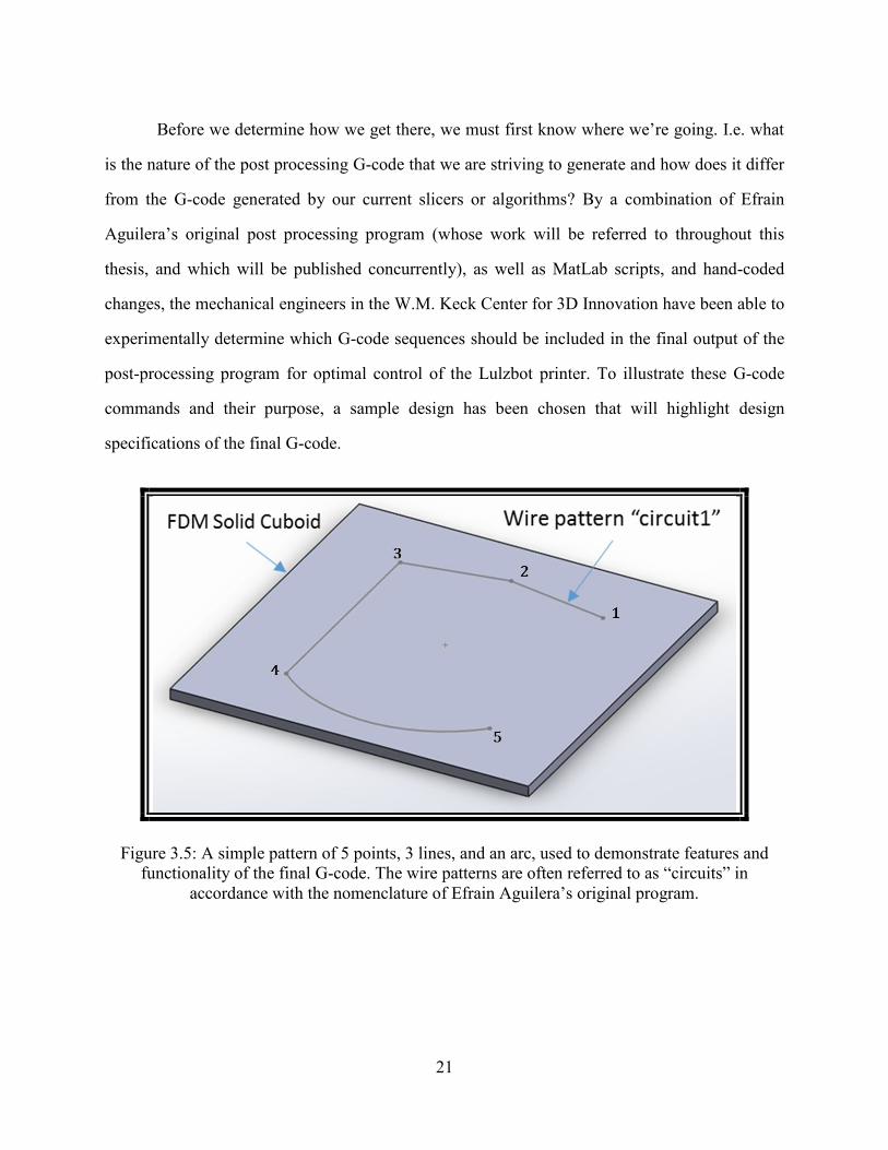
Figure 3.5: A simple pattern of 5 points, 3 lines, and an arc, used to demonstrate features and
functionality of the final G-code. The wire patterns are often referred to as “circuits” in
accordance with the nomenclature of Efrain Aguilera’s original program.
22
Tool initialization
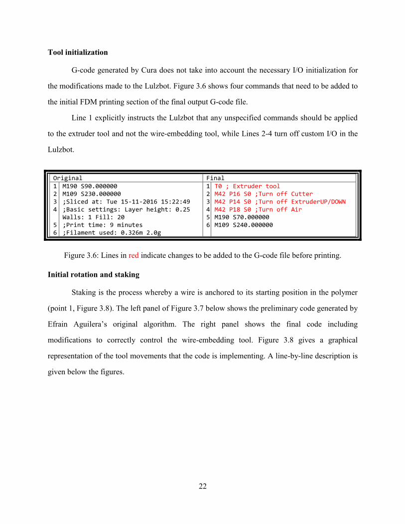
G-code generated by Cura does not take into account the necessary I/O initialization for
the modifications made to the Lulzbot. Figure 3.6 shows four commands that need to be added to
the initial FDM printing section of the final output G-code file.
Line 1 explicitly instructs the Lulzbot that any unspecified commands should be applied
to the extruder tool and not the wire-embedding tool, while Lines 2-4 turn off custom I/O in the
Lulzbot.
Original Final 1 2 3 4 5 6
M190 S90.000000 M109 S230.000000 ;Sliced at: Tue 15-11-2016 15:22:49 ;Basic settings: Layer height: 0.25 Walls: 1 Fill: 20 ;Print time: 9 minutes ;Filament used: 0.326m 2.0g
1 2 3 4 5 6
T0 ; Extruder tool M42 P16 S0 ;Turn off Cutter M42 P14 S0 ;Turn off ExtruderUP/DOWN M42 P18 S0 ;Turn off Air M190 S70.000000 M109 S240.000000
Figure 3.6: Lines in red indicate changes to be added to the G-code file before printing.
Initial rotation and staking
Staking is the process whereby a wire is anchored to its starting position in the polymer
(point 1, Figure 3.8). The left panel of Figure 3.7 below shows the preliminary code generated by
Efrain Aguilera’s original algorithm. The right panel shows the final code including
modifications to correctly control the wire-embedding tool. Figure 3.8 gives a graphical
representation of the tool movements that the code is implementing. A line-by-line description is
given below the figures.
23
Aguilera algorithm Final 1 2 3 4 5 6 7 8
(* SHAPE Nr: 0 *) G0 X177.878 Y71.273 M3 M8 G0 Z 3.000 F150 G1 Z 0.000 F400 G1 X163.716 Y73.770
1 2 3 4 5 6 7 8 9 10 11 12 13 14 15
;(* SHAPE Nr: 0 *) G0 F320 X177.878 Y71.273 M3 M8 G1 F80 E3.01777; tool rotation added by Python/addToolRotation G0 F320 Z4.425 F150 G1 F320 Z1.425 G4 P1000; Dwell G1 F320 Z1.925 M42 P18 S0; Air off G4 P200; Dwell M42 P18 S255; Air on G4 P2500; Dwell M42 P18 S0; Air off G4 P1000; Dwell G1 F320 Z1.425 F400 G1 F320 X163.716 Y73.770
Figure 3.7: The staking process in G-code: lines in red show changes made to correctly control
the Lulzbot wire-embedding tool.
Figure 3.8: Graphical representation from Solidworks of the wire-pattern being implemented by
the G-code in Figure 3.7. This code specifies tool orientation, staking at point 1, and translating
and embedding wire to point 2 (highlighted in red).
24
In the right pane of Figure 3.7, line 1 has been changed to a comment, line 2 has been
modified to explicitly define movement speed (F320), and a number of undesired lines have been
removed. In line 3, a rotation command is specified. As this is the first tool orientation to be
specified by the code, it is defined as an absolute rotation value (axis of rotation is the Z-axis),
where 0° corresponds to the Y-axis (indicated by the blue dashed line in Figure 3.8). The
orientation required to embed the first line of wire is 280°, which corresponds to an E parameter
of E3.02 (see Figure 3.8). This rotation is performed high above the polymer surface, before the
tool is commanded to begin to descend in line 4. In line 5, the wire-embedding tool head
descends again and comes into contact with the polymer surface (point 1 in Figure 3.8). The tool
delays for 1000 ms in line 6 and then raises back up 0.5 mm in line 7. Lines 8-12 initiate a 2500
ms blast of air to cool the polymer surface below its glass transition temperature, securing the
wire in position in the polymer. Line 13 implements another 1000 ms delay, followed by a 0.5
mm descent in the Z direction to return the tool-head to the polymer surface in line 14 (point 1
again). The tool then immediately begins to translate to the next co-ordinate (point 2), line 15,
with wire being pulled and embedded into the polymer as the tool travels away from the staking
location.
Additional rotation processing requirements
The next two steps in this pattern demonstrate a peculiarity in how angles of different
sizes need to be handled differently. The first turn, at point 2, involves a relative change in
direction of 20°, whilst the second turn goes through an angle of 80°. Experimental observation
has determined that angle changes of greater than approximately 30° in the polymer plane often
result in undesirable effects. One such effect is that the wire is too hot to embed at the vertex of
the turn and can be dragged into a gradual curve, instead of creating the desired sharp turn at the
vertex. To compensate, additional steps are taken at vertices where turns greater than 30° occur.
The sequence of steps involves raising the tool from the polymer plane, followed by cooling, a
25
mid-air rotation, and returning the tool back to the original position. Figure 3.9 and Figure 3.10
illustrate the sequence.
Aguilera algorithm Final 8 9 10
G1 X163.716 Y73.770 G1 X149.554 Y71.273 G1 X149.554 Y41.273
15 16 17 18 19 20 21 22 23 24 25 26 27 28 29 30 31
G1 F320 X163.716 Y73.770 G91 G1 F80 E-0.21554; tool rotation added by Python/addToolRotation G90 G1 F320 X149.554 Y71.273 G1 F320 X149.505 Y71.264 Z1.925; tool taper added by Python/genTaperLine M42 P18 S0; Air off G4 P200; Dwell M42 P18 S255; Air on G4 P2000; Dwell M42 P18 S0; Air off G91 G1 F80 E-0.86223; tool rotation added by Python/addToolRotation G90 G1 F320 X149.554 Y71.273 G4 P1000; Dwell G1 F320 Z1.425 G1 F320 X149.554 Y41.273
Figure 3.9: Small and large rotations implemented in G-code: lines in red show changes made to
correctly control the Lulzbot wire-embedding tool.
26
Figure 3.10: Graphical representation of the small (point 2) and large (points 3 and 4) rotations
required by the wire-pattern. Turns at points 2 and 3 and the translational lines in red are
generated by the G-code in Figure 3.9.
The sequence starts at line 15 (point 2), the endpoint for the sequence in Figure 3.7. At
this point, a rotation of 20° is required. Since the rotation is less than 30°, the rotation can be
made without lifting the tool from the polymer plane. Lines 16-18 achieve this by switching to
relative positioning, initiating a counterclockwise (CCW) turn of 20° (-20°/360° * E3.88 = E-
0.216), and switching back to absolute positioning. Line 19 instructs the tool to translate to point
3, embedding wire as it travels. At point 3, we encounter a turn of 80°. Line 20 instructs the tool
to continue for 0.05 mm in the same XY direction (a relative change of X-0.049 Y-0.009), whilst
simultaneously traveling up 0.5 mm in the Z direction, above the polymer plane. Lines 21-25
instruct the cooling air to blow for 2000 ms. Lines 26-28 command the 80° CCW rotation. Line
29 commands the tool to return to its original XY location in line 19 (point 3). Line 30 instructs
the tool to descend back to the polymer surface, before continuing to point 4 in line 31.
G2 and G3 arc processing
G2 and G3 G-code commands specify clockwise and counterclockwise arcs respectively.
In the example below, the syntax of the command is G3 X177.878 Y41.273 I14.162 J15.204,
wherein “G3” specifies CCW rotation, “X177.878 Y41.273” specifies the end coordinates of the
curve (point 5), and “I14.162 J15.204” specifies the vector to get from the start of the arc (line
10, point 4: G1 X149.554 Y41.273) to the origin (Figure 3.12). However, G2 and G3 commands
are not recognized by the Lulzbot G-code parser, so these arcs must be interpreted into a series of
G1 translational commands and then reprocessed to append the appropriate rotation commands.
27
Aguilera algorithm with simulated
absolute coordinates2
Final
10 11
G1 X149.554 Y41.273 G3 X177.878 Y41.273 I14.162 J15.204
31 32 33 34 35 36 37 38 39 40 41 42 43 44 45 46 47 48 ... 165 166 167 168
G1 F320 X149.554 Y41.273 G1 F320 X149.554 Y41.223 Z1.925; tool taper added by Python/genTaperLine M42 P18 S0; Air off G4 P200; Dwell M42 P18 S255; Air on G4 P2000; Dwell M42 P18 S0; Air off G91 G1 F80 E-0.52133; tool rotation added by Python/addToolRotation G90 G1 F320 X149.554 Y41.273 G4 P1000; Dwell G1 F320 Z1.425 G1 F320 X150.282 Y40.626 G91 G1 F80 E-0.02883; tool rotation added by Python/addToolRotation G90 G1 F320 X151.039 Y40.014 ... G91 G1 F80 E-0.02883; tool rotation added by Python/addToolRotation G90 G1 F320 X177.878 Y41.273
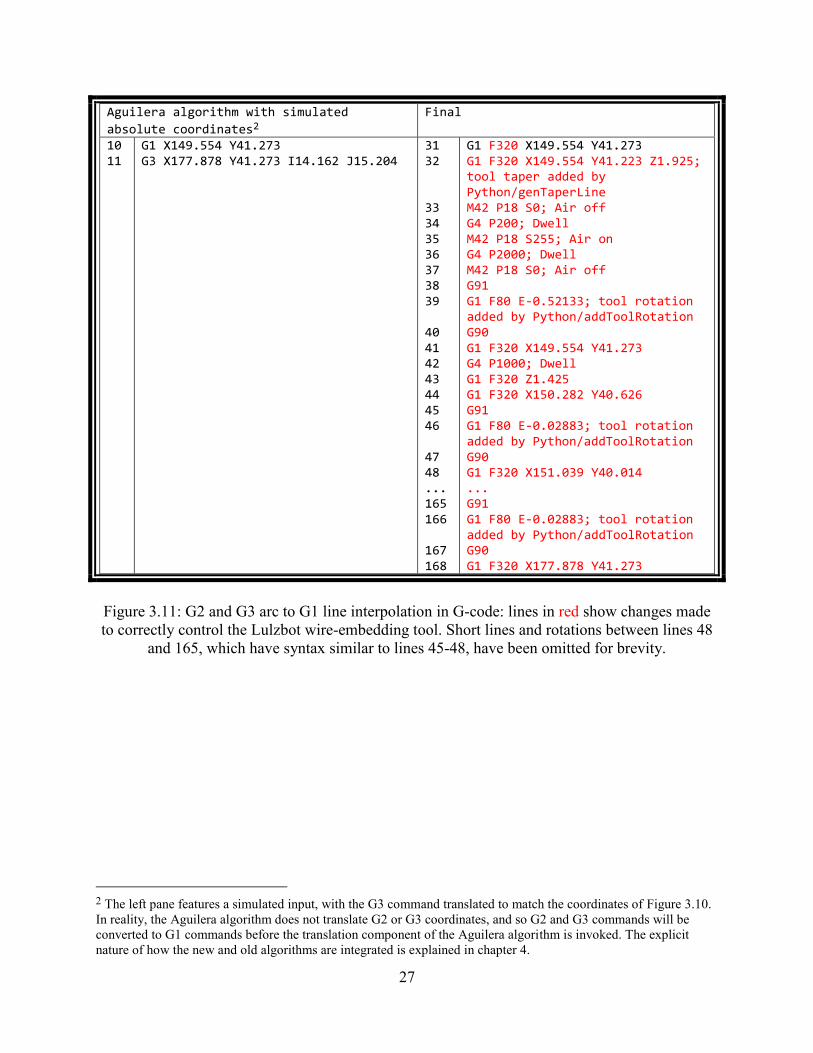
Figure 3.11: G2 and G3 arc to G1 line interpolation in G-code: lines in red show changes made
to correctly control the Lulzbot wire-embedding tool. Short lines and rotations between lines 48
and 165, which have syntax similar to lines 45-48, have been omitted for brevity.
2 The left pane features a simulated input, with the G3 command translated to match the coordinates of Figure 3.10.
In reality, the Aguilera algorithm does not translate G2 or G3 coordinates, and so G2 and G3 commands will be
converted to G1 commands before the translation component of the Aguilera algorithm is invoked. The explicit
nature of how the new and old algorithms are integrated is explained in chapter 4.
28
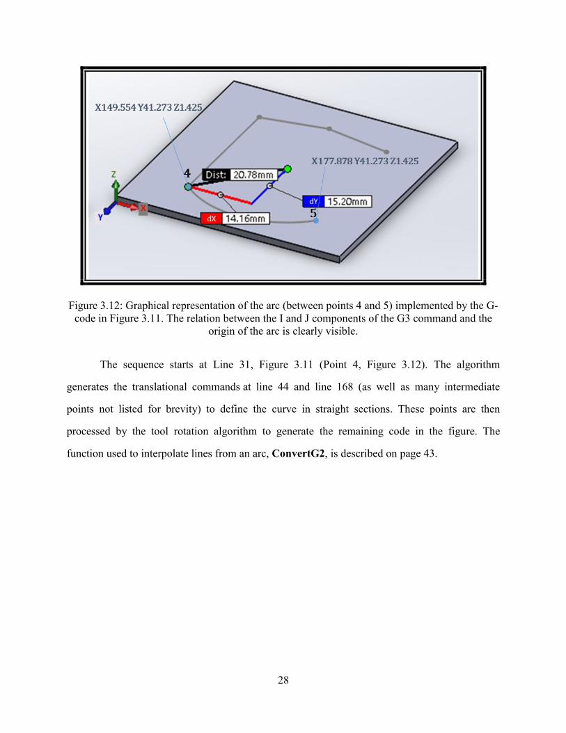
Figure 3.12: Graphical representation of the arc (between points 4 and 5) implemented by the G-
code in Figure 3.11. The relation between the I and J components of the G3 command and the
origin of the arc is clearly visible.
The sequence starts at Line 31, Figure 3.11 (Point 4, Figure 3.12). The algorithm
generates the translational commands at line 44 and line 168 (as well as many intermediate
points not listed for brevity) to define the curve in straight sections. These points are then
processed by the tool rotation algorithm to generate the remaining code in the figure. The
function used to interpolate lines from an arc, ConvertG2, is described on page 43.
29
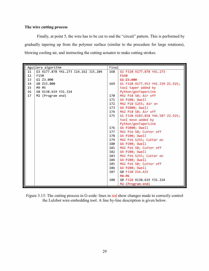
The wire cutting process
Finally, at point 5, the wire has to be cut to end the “circuit” pattern. This is performed by
gradually tapering up from the polymer surface (similar to the procedure for large rotations),
blowing cooling air, and instructing the cutting actuator to make cutting strokes.
Aguilera algorithm Final 11 12 13 14 15 16 17
G3 X177.878 Y41.273 I14.162 J15.204 F150 G1 Z3.000 G0 Z15.000 M9 M5 G0 X138.619 Y31.324 M2 (Program end)
168 169 170 171 172 173 174 175 176 177 178 179 180 181 182 183 184 185 186 187 188
G1 F320 X177.878 Y41.273 F150 G1 Z3.000 G1 F320 X177.953 Y41.339 Z1.925; tool taper added by Python/genTaperLine M42 P18 S0; Air off G4 P200; Dwell M42 P18 S255; Air on G4 P2000; Dwell M42 P18 S0; Air off G1 F320 X183.858 Y46.587 Z2.925; tool move added by Python/genTaperLine G4 P2000; Dwell M42 P16 S0; Cutter off G4 P200; Dwell M42 P16 S255; Cutter on G4 P200; Dwell M42 P16 S0; Cutter off G4 P200; Dwell M42 P16 S255; Cutter on G4 P200; Dwell M42 P16 S0; Cutter off G4 P200; Dwell G0 F320 Z16.425 M9 M5 G0 F320 X138.619 Y31.324 M2 (Program end)
Figure 3.13: The cutting process in G-code: lines in red show changes made to correctly control
the Lulzbot wire-embedding tool. A line by-line description is given below.
30
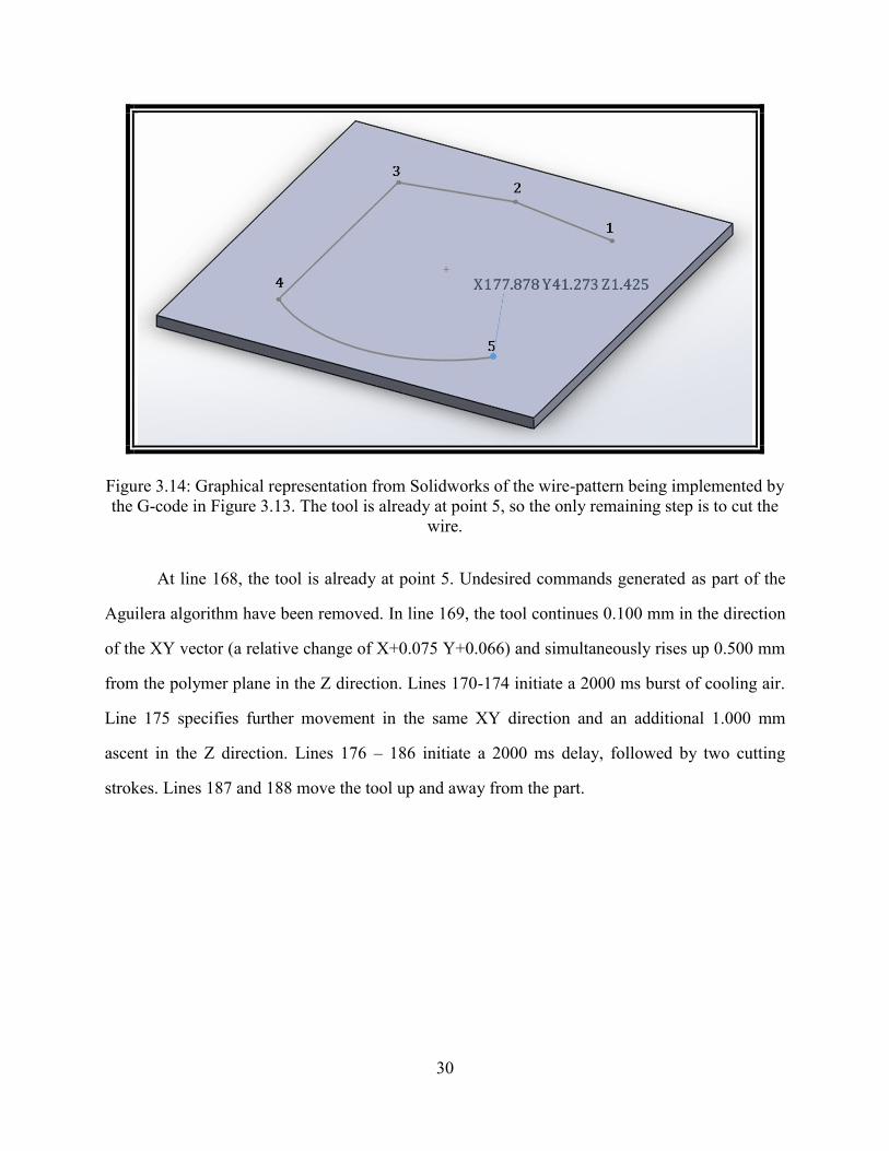
Figure 3.14: Graphical representation from Solidworks of the wire-pattern being implemented by
the G-code in Figure 3.13. The tool is already at point 5, so the only remaining step is to cut the
wire.
At line 168, the tool is already at point 5. Undesired commands generated as part of the
Aguilera algorithm have been removed. In line 169, the tool continues 0.100 mm in the direction
of the XY vector (a relative change of X+0.075 Y+0.066) and simultaneously rises up 0.500 mm
from the polymer plane in the Z direction. Lines 170-174 initiate a 2000 ms burst of cooling air.
Line 175 specifies further movement in the same XY direction and an additional 1.000 mm
ascent in the Z direction. Lines 176 – 186 initiate a 2000 ms delay, followed by two cutting
strokes. Lines 187 and 188 move the tool up and away from the part.
31
Foundation layer generation
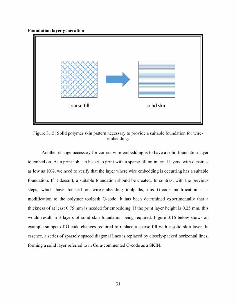
Figure 3.15: Solid polymer skin pattern necessary to provide a suitable foundation for wire-
embedding.
Another change necessary for correct wire-embedding is to have a solid foundation layer
to embed on. As a print job can be set to print with a sparse fill on internal layers, with densities
as low as 10%, we need to verify that the layer where wire embedding is occurring has a suitable
foundation. If it doesn’t, a suitable foundation should be created. In contrast with the previous
steps, which have focused on wire-embedding toolpaths, this G-code modification is a
modification to the polymer toolpath G-code. It has been determined experimentally that a
thickness of at least 0.75 mm is needed for embedding. If the print layer height is 0.25 mm, this
would result in 3 layers of solid skin foundation being required. Figure 3.16 below shows an
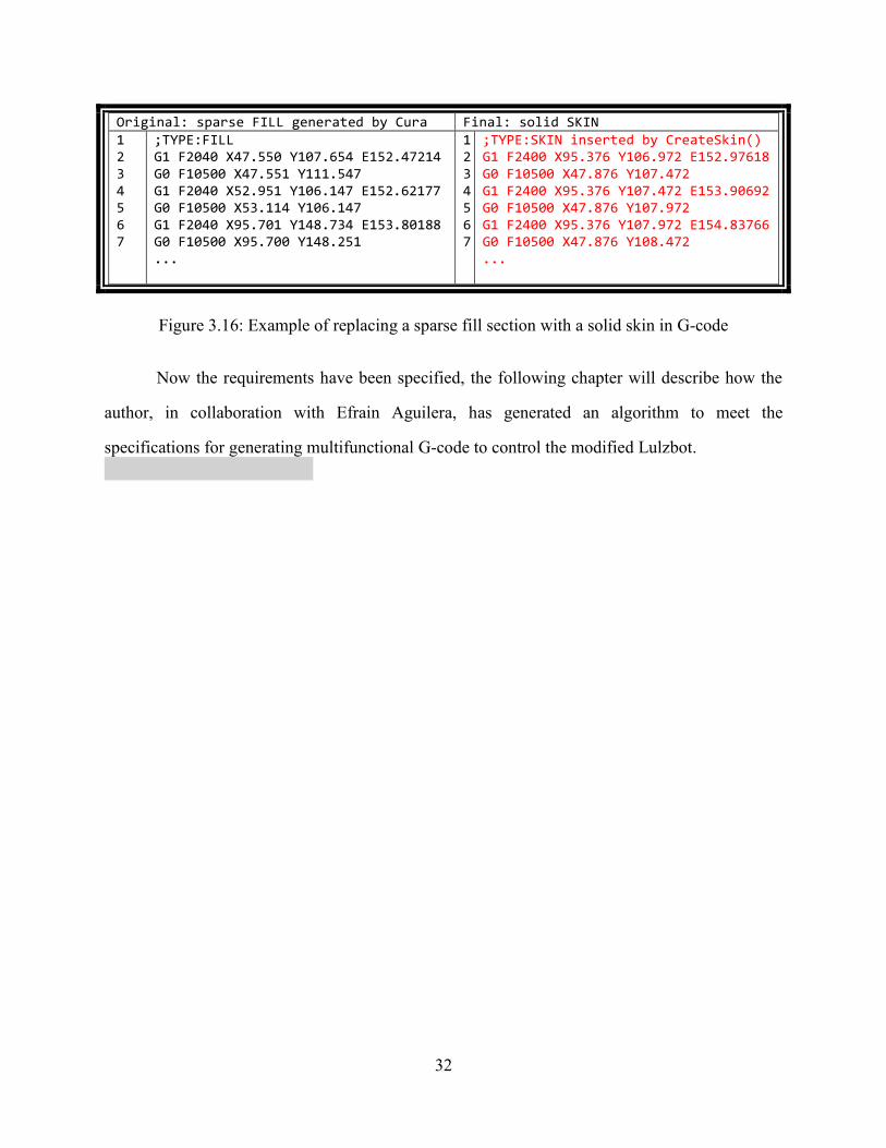
example snippet of G-code changes required to replace a sparse fill with a solid skin layer. In
essence, a series of sparsely spaced diagonal lines is replaced by closely-packed horizontal lines,
forming a solid layer referred to in Cura-commented G-code as a SKIN.
32
Original: sparse FILL generated by Cura Final: solid SKIN 1 2 3 4 5 6 7
;TYPE:FILL G1 F2040 X47.550 Y107.654 E152.47214 G0 F10500 X47.551 Y111.547 G1 F2040 X52.951 Y106.147 E152.62177 G0 F10500 X53.114 Y106.147 G1 F2040 X95.701 Y148.734 E153.80188 G0 F10500 X95.700 Y148.251 ...
1 2 3 4 5 6 7
;TYPE:SKIN inserted by CreateSkin() G1 F2400 X95.376 Y106.972 E152.97618 G0 F10500 X47.876 Y107.472 G1 F2400 X95.376 Y107.472 E153.90692 G0 F10500 X47.876 Y107.972 G1 F2400 X95.376 Y107.972 E154.83766 G0 F10500 X47.876 Y108.472 ...
Figure 3.16: Example of replacing a sparse fill section with a solid skin in G-code
Now the requirements have been specified, the following chapter will describe how the
author, in collaboration with Efrain Aguilera, has generated an algorithm to meet the
specifications for generating multifunctional G-code to control the modified Lulzbot.
33
Chapter 4: A method for generating multifunctional G-code
Introduction
As outlined in chapters 1 and 2, the generic STL file format typically used to define solid
bodies for 3D printing lacks the ability to fully define a multi-process 3D print. In response to
this, the file must either be replaced with a more sophisticated file format or augmented by
generating additional files to supplement the STL file and provide the information lacking in the
STL file, such as toolpath information for the wire-embedding tool. As one design constraint is
to integrate with existing Solidworks design software, a solution had to be found that was
compatible with Solidworks capabilities. While Solidworks does offer native support for
generating AMF files, the only additional information that can be specified in the file is material
color and type, which is inadequate for a process such as wire-embedding. As Solidworks offers
a Visual Basic API (application program interface), it may be possible to develop an AMF-
exporting macro in the Visual Basic programming language. However, as there is limited access
to software libraries that are compatible with the Solidworks Visual Basic API implementation, a
simpler approach was adopted. This approach, developed by Efrain Aguilera [27], involves
augmenting the STL file with additional files that contain the information necessary to fully
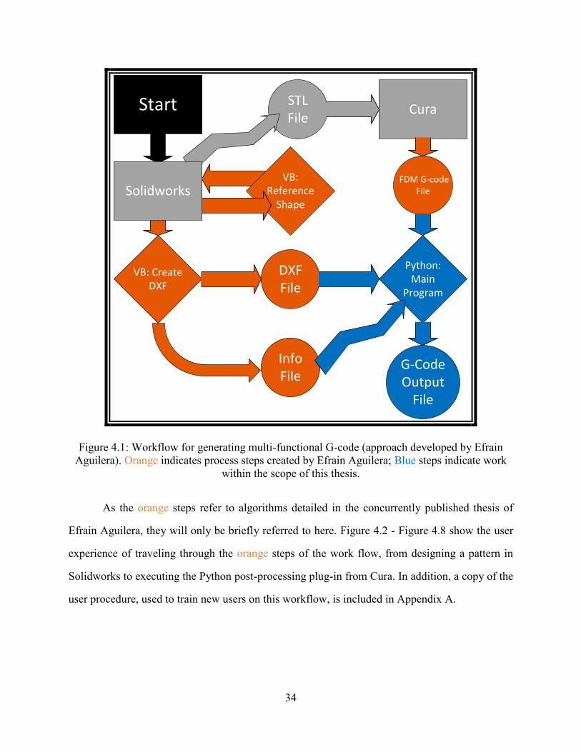
define a multi-process, wire-embedding, FDM print. Outlined in Figure 4.1 below, the process
involves the generation of an STL file with FDM print information and a DXF file with wire-
embedding information, both of which contain a reference shape (generated by a Visual Basic
macro), to preserve the translational and rotational geometric information between components.
An info.txt file is generated, containing the Z-height for each wire-embedding sub-task3.
3 The current implementation only supports wire-patterns parallel to the XY plane.
34
CuraSTLFile
VB: Create DXF
DXFFile
InfoFile
Python: Main
Program
G-CodeOutput
File
Start
FDM G-codeFile
VB: Reference
ShapeSolidworks
Figure 4.1: Workflow for generating multi-functional G-code (approach developed by Efrain
Aguilera). Orange indicates process steps created by Efrain Aguilera; Blue steps indicate work
within the scope of this thesis.
As the orange steps refer to algorithms detailed in the concurrently published thesis of
Efrain Aguilera, they will only be briefly referred to here. Figure 4.2 - Figure 4.8 show the user
experience of traveling through the orange steps of the work flow, from designing a pattern in
Solidworks to executing the Python post-processing plug-in from Cura. In addition, a copy of the
user procedure, used to train new users on this workflow, is included in Appendix A.
35
Figure 4.2: A conventional, 3D-printable design is created in Solidworks.
Figure 4.3: A 3D Sketch4 representing the wire pattern is created and each subsequent wire
pattern sketch is renamed to circuit1, circuit2, circuit3… as appropriate.
4 “3D” as this explicitly defines the sketch in x, y, and z as opposed to a conventional sketch, which only has 2D
data explicitly within the sketch and requires a reference to the surface it is drawn on to complete its definition. The
explicit x, y, z definition in the 3D sketch is useful in the next step
36
Figure 4.4: A Visual Basic macro is run, which creates a reference part (top of the figure).
A second Visual Basic macro is run, which exports each circuit pattern and reference geometry
as individual DXF files labeled circuit1 (Top).dxf, circuit2 (Top).dxf, circuit3 (Top).dxf,
respectively (when more than one wire pattern is present). The FDM part is saved as an STL file.
Figure 4.5: Depiction of the DXF file information outputted by the Solidworks Visual Basic
macro, featuring the reference geometry.
37
Figure 4.6: The STL file is loaded into the Cura slicing software and the America Makes II
Python plugin is loaded from the plugins tab.
Figure 4.7: The Python plugin opens the Python main post-processing program and a GUI where
various processing parameters relating to the multi-process print can be configured. The G-code
is generated by clicking Circuit.5
5 Edit boxes containing wire-embedding processing parameters indicate a later modification to the GUI from the
original Aguilera GUI. Parameter edit boxes were added to the GUI by Jake Lasley.
38
Figure 4.8: Multiple files are generated during the processing steps.
MagneticCoilRo – Complete.gcode contains the complete print job, while the
MagneticCoilRo – [1,2,3] – [Polymer,Circuit].gcode files allow individual stages to be printed
separately.
The Python G-code Post-processor
A collaboration
The work on the Python G-code processor has been highly collaborative in nature. To
help credit the work of the different contributors, the flowcharts and diagrams outlining the
algorithm have been color coded to highlight who contributed to each step. Some hierarchical
organization changes and variable name changes have occurred with respect to the code in Efrain
Aguilera’s concurrent publication, but do not affect the internal function of his algorithms.
AmericaMakes.py
AmericaMakes.py is a Python plug-in for Cura that initializes the post processor. The
script initializes an executable that prompts the user for the file path of the folder where the files
in Figure 4.8 were generated and saves the file path information in a variable, “out”. The script
39
then uses the Cura slicer to generate G-code for the FDM print (without any wire-embedding
information) and places this G-code in a file called temp.gcode in the folder designated by the
“out” variable.
It then initializes and passes the “out” value to another executable, main.exe (which was
compiled from a Python script, main.py).
main.py
Figure 4.9: Early version of the GUI, developed by Efrain Aguilera.
Originally developed by Efrain Aguilera, the main.py script initializes a GUI that guides
the user through the code generation progress. The GUI has been modified by Jake Lasley to
include access to wire-processing parameters (Figure 4.7 above). The user starts G-code
generation by selecting the Circuit button. The main.py script then begins to parse the input files
info.txt, circuit 1 (Top).dxf, and temp.gcode generated in the earlier steps (Figure 4.10 below). It
starts by reading info.txt, which was generated by the Solidworks macro and contains the
information about the z height that each “circuit” or wire-pattern is found at. These height values
in mm are stored in a list, circuitZheights, for later use. The script then uses the length of list
circuitZheights to determine how many circuits are present and then initializes a loop to convert
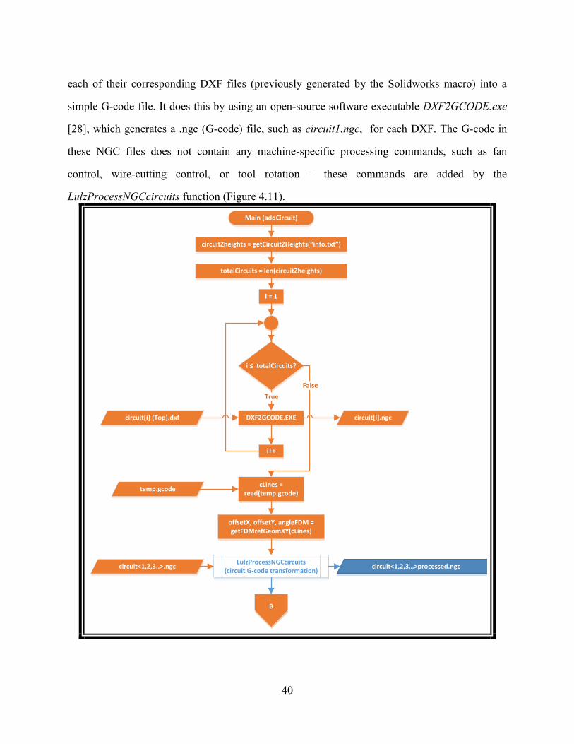
40
each of their corresponding DXF files (previously generated by the Solidworks macro) into a
simple G-code file. It does this by using an open-source software executable DXF2GCODE.exe
[28], which generates a .ngc (G-code) file, such as circuit1.ngc, for each DXF. The G-code in
these NGC files does not contain any machine-specific processing commands, such as fan
control, wire-cutting control, or tool rotation – these commands are added by the
LulzProcessNGCcircuits function (Figure 4.11).
Main (addCircuit)
circuit[i].ngc
i � totalCircuits?
DXF2GCODE.EXE
False
True
i = 1
circuit[i] (Top).dxf
cLines = read(temp.gcode)
temp.gcode
offsetX, offsetY, angleFDM = getFDMrefGeomXY(cLines)
LulzProcessNGCcircuits(circuit G-code transformation)
circuit<1,2,3 processed.ngccircuit<1,2,3..>.ngc
i++
BB
circuitZheights = getCircuitZHeights( info.txt
totalCircuits = len(circuitZheights)
41
Figure 4.10: Overview (1 of 3) of the steps of the addCircuit function of the main.py program.
Orange indicates process steps created by Efrain Aguilera; Blue indicates process steps
developed within the scope of this publication. Part B continues in Figure 4.17, page 53.
The LulzProcessNGCcircuits function
LulzProcessNGCcircuits
circuit[j].ngc
j � totalCircuits
Read circuit[j].ngc into lines
returnFalse
True
G2 or G3 commands
present?
Add F speeds to G1 commands
Write lines into circuit[j]processed.ngc
circuit[j]processed.ngc
False
j++
j = 1
Convert G2/G3 commands to G1
True
Aguilera Procrustes Translation
Add Tool Rotation
Add Staking
Add Cutting
Clean unrecognized commands
translate circuit Z values
42
Figure 4.11: Overview of the LulzProcessNGCcircuits algorithm which generates wire-extruding
G-code for the modified Lulzbot. Orange indicate steps generated by Efrain Aguilera. Blue steps
relate to this publication. In this algorithm, the input is the circuit[j].ngc file generated by
DXF2GCODE.exe; the output is the circuit[j]processed.ngc file which contains correctly-
formatted G-code for each circuit pattern.
The LulzProcessNGCcircuits function takes the basic G-code output by
DFX2GCODE.exe and processes it, so that it can be correctly parsed by the modified Lulzbot
printer. It does this by setting up a loop to apply the function sequentially to each of the circuit
patterns generated. The first step of the body of the loop reads the basic G-code output of
DXF2GCODE.exe into a list called lines. It then scans the list for any occurrence of G2 or G3
text, indicating a G2 or G3 arc command is present, which needs to be replaced. If found, the
lines list is passed into the convertG2 function (Figure 4.12).
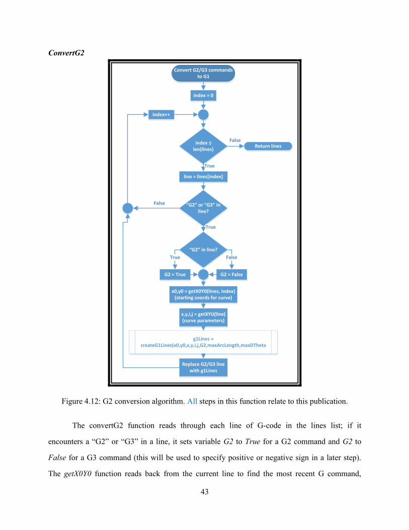
43
ConvertG2
Convert G2/G3 commands to G1
index � len(lines)
line = lines[index]
Return linesFalse
True
G2 or G3 in line?
x,y,i,j = getXYIJ(line)(curve parameters)
True
index++
index = 0
x0,y0 = getX0Y0(lines, index)(starting coords for curve)
False
G2 in line?
G2 = True G2 = False
FalseTrue
g1Lines = createG1Lines(x0,y0,x,y,i,j,G2,maxArcLength,maxDTheta
Replace G2/G3 line with g1Lines
Figure 4.12: G2 conversion algorithm. All steps in this function relate to this publication.
The convertG2 function reads through each line of G-code in the lines list; if it
encounters a “G2” or “G3” in a line, it sets variable G2 to True for a G2 command and G2 to
False for a G3 command (this will be used to specify positive or negative sign in a later step).
The getX0Y0 function reads back from the current line to find the most recent G command,
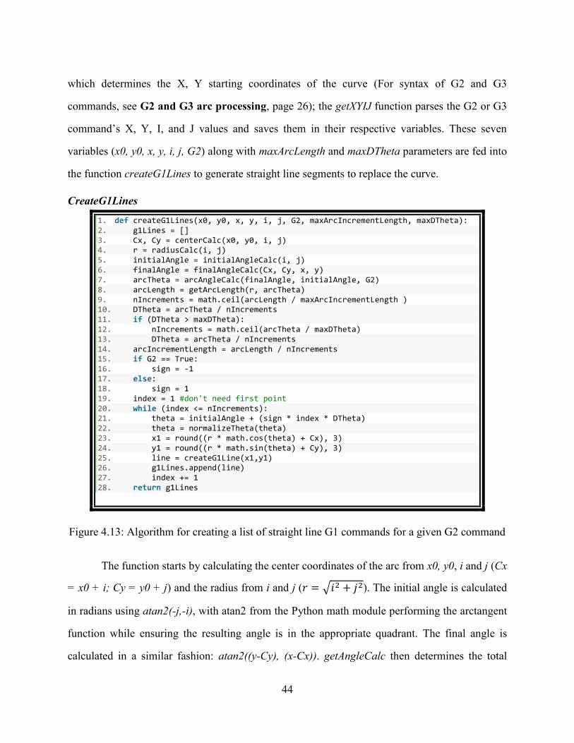
44
which determines the X, Y starting coordinates of the curve (For syntax of G2 and G3
commands, see G2 and G3 arc processing, page 26); the getXYIJ function parses the G2 or G3
command’s X, Y, I, and J values and saves them in their respective variables. These seven
variables (x0, y0, x, y, i, j, G2) along with maxArcLength and maxDTheta parameters are fed into
the function createG1Lines to generate straight line segments to replace the curve.
CreateG1Lines
1. def createG1Lines(x0, y0, x, y, i, j, G2, maxArcIncrementLength, maxDTheta): 2. g1Lines = [] 3. Cx, Cy = centerCalc(x0, y0, i, j) 4. r = radiusCalc(i, j) 5. initialAngle = initialAngleCalc(i, j) 6. finalAngle = finalAngleCalc(Cx, Cy, x, y) 7. arcTheta = arcAngleCalc(finalAngle, initialAngle, G2) 8. arcLength = getArcLength(r, arcTheta) 9. nIncrements = math.ceil(arcLength / maxArcIncrementLength ) 10. DTheta = arcTheta / nIncrements 11. if (DTheta > maxDTheta): 12. nIncrements = math.ceil(arcTheta / maxDTheta) 13. DTheta = arcTheta / nIncrements 14. arcIncrementLength = arcLength / nIncrements 15. if G2 == True: 16. sign = -1 17. else: 18. sign = 1 19. index = 1 #don't need first point 20. while (index <= nIncrements): 21. theta = initialAngle + (sign * index * DTheta) 22. theta = normalizeTheta(theta) 23. x1 = round((r * math.cos(theta) + Cx), 3) 24. y1 = round((r * math.sin(theta) + Cy), 3) 25. line = createG1Line(x1,y1) 26. g1Lines.append(line) 27. index += 1 28. return g1Lines
Figure 4.13: Algorithm for creating a list of straight line G1 commands for a given G2 command
The function starts by calculating the center coordinates of the arc from x0, y0, i and j (Cx
= x0 + i; Cy = y0 + j) and the radius from i and j (𝑟 = √𝑖2 + 𝑗2). The initial angle is calculated
in radians using atan2(-j,-i), with atan2 from the Python math module performing the arctangent
function while ensuring the resulting angle is in the appropriate quadrant. The final angle is
calculated in a similar fashion: atan2((y-Cy), (x-Cx)). getAngleCalc then determines the total
45
angle being turned through based on the initial and final angles and whether the turn is clockwise
(G2 = True) or counterclockwise (G2 = False). The arc length is then calculated from the radius
and arc angle. It then calculates the number of increments to split the arc into by dividing
arcLength by maxArcIncrement length and then rounding up to the nearest integer. In the case of
the default maxArcIncrement length of 1.0 mm, this will result in segments slightly shorter than
1 mm, due to the rounding up. It then divides the arcAngle by nIncrements to determine the theta
value traveled through in each segment. If this angle is too large (greater than 10° by default), the
increments will be recalculated to ensure the generated lines have sufficient resolution to
accurately represent the curve. The arcIncrementLength of an individual line is then determined
by dividing arcLength / nIncrements. A loop is then set up to calculate the coordinates for each
point, based on their r, theta polar coordinates from Cx, Cy. The parameter r is constant for any
given arc and theta varies by initialAngle + (sign * index * DTheta), with the index incrementing
on each loop iteration. The polar coordinates are converted into Cartesian values and stored in
x1, y1 variables. These variables are then used to generate G1 lines with standard G-code syntax
(although no F value for wire-embedding speed has been explicitly defined at this point). Each
line is appended to the g1Lines list to return back up to the parent convertG2 function. The final
step of the convertG2 function replaces the original G2 or G3 command with the contents of the
g1Lines list.
X, Y, Z translations and F wire-embedding speed
Returning to Figure 4.11, the LulzProcessNGCcircuits algorithm continues by
performing a Procrustes translation function (detailed in Efrain Aguilera’s thesis), which
translates the G0 and G1 commands to their correct locations relative to the FDM temp.gcode
and the XY tool offsets. As the G2 and G3 commands have already been converted to G1, these
commands are also correctly translated. However, the Z values are ignored by the Aguilera
Procrustes Translation and must be adjusted by a separate function, transformCircuitZ(lines,
zHeight). This function acts on all lines and modifies Z values by adding the zHeight of the
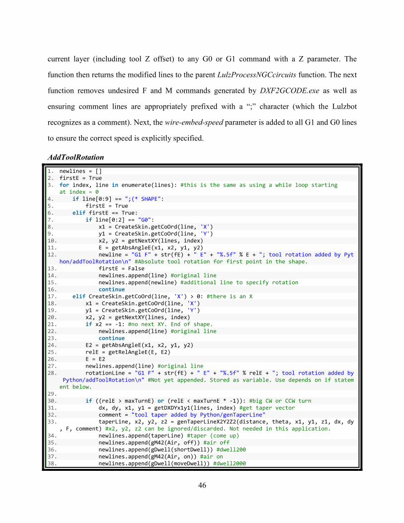
46
current layer (including tool Z offset) to any G0 or G1 command with a Z parameter. The
function then returns the modified lines to the parent LulzProcessNGCcircuits function. The next
function removes undesired F and M commands generated by DXF2GCODE.exe as well as
ensuring comment lines are appropriately prefixed with a “;” character (which the Lulzbot
recognizes as a comment). Next, the wire-embed-speed parameter is added to all G1 and G0 lines
to ensure the correct speed is explicitly specified.
AddToolRotation
1. newlines = [] 2. firstE = True 3. for index, line in enumerate(lines): #this is the same as using a while loop starting
at index = 0 4. if line[0:9] == ";(* SHAPE": 5. firstE = True 6. elif firstE == True: 7. if line[0:2] == "G0": 8. x1 = CreateSkin.getCoOrd(line, 'X') 9. y1 = CreateSkin.getCoOrd(line, 'Y') 10. x2, y2 = getNextXY(lines, index) 11. E = getAbsAngleE(x1, x2, y1, y2) 12. newline = "G1 F" + str(fE) + " E" + "%.5f" % E + "; tool rotation added by Pyt
hon/addToolRotation\n" #Absolute tool rotation for first point in the shape. 13. firstE = False 14. newlines.append(line) #original line 15. newlines.append(newline) #additional line to specify rotation 16. continue 17. elif CreateSkin.getCoOrd(line, 'X') > 0: #there is an X 18. x1 = CreateSkin.getCoOrd(line, 'X') 19. y1 = CreateSkin.getCoOrd(line, 'Y') 20. x2, y2 = getNextXY(lines, index) 21. if x2 == -1: #no next XY. End of shape. 22. newlines.append(line) #original line 23. continue 24. E2 = getAbsAngleE(x1, x2, y1, y2) 25. relE = getRelAngleE(E, E2) 26. E = E2 27. newlines.append(line) #original line 28. rotationLine = "G1 F" + str(fE) + " E" + "%.5f" % relE + "; tool rotation added by
Python/addToolRotation\n" #Not yet appended. Stored as variable. Use depends on if statement below.
29. 30. if ((relE > maxTurnE) or (relE < maxTurnE * -1)): #big CW or CCW turn 31. dx, dy, x1, y1 = getDXDYx1y1(lines, index) #get taper vector 32. comment = "tool taper added by Python/genTaperLine" 33. taperLine, x2, y2, z2 = genTaperLineX2Y2Z2(distance, theta, x1, y1, z1, dx, dy
, F, comment) #x2, y2, z2 can be ignored/discarded. Not needed in this application. 34. newlines.append(taperLine) #taper (come up) 35. newlines.append(gM42(Air, off)) #air off 36. newlines.append(gDwell(shortDwell)) #dwell200 37. newlines.append(gM42(Air, on)) #air on 38. newlines.append(gDwell(moveDwell)) #dwell2000
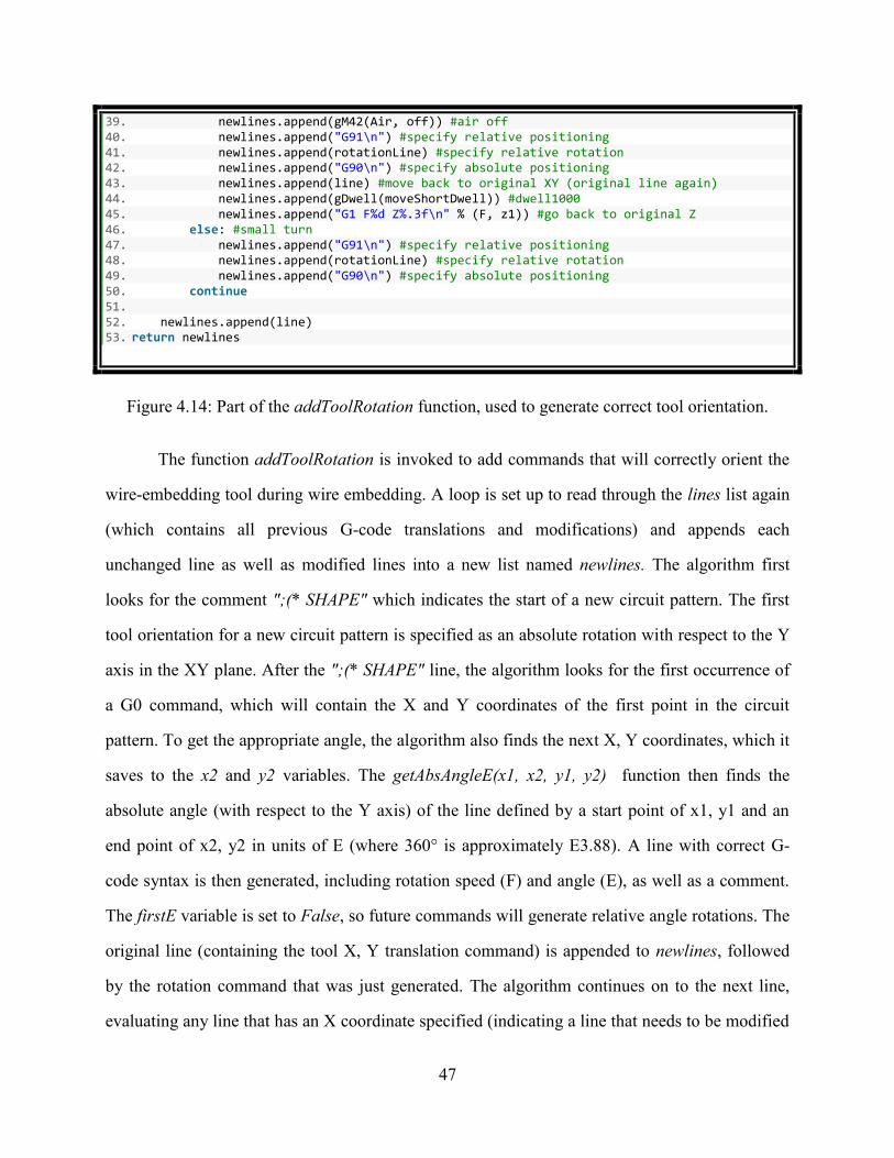
47
39. newlines.append(gM42(Air, off)) #air off 40. newlines.append("G91\n") #specify relative positioning 41. newlines.append(rotationLine) #specify relative rotation 42. newlines.append("G90\n") #specify absolute positioning 43. newlines.append(line) #move back to original XY (original line again) 44. newlines.append(gDwell(moveShortDwell)) #dwell1000 45. newlines.append("G1 F%d Z%.3f\n" % (F, z1)) #go back to original Z 46. else: #small turn 47. newlines.append("G91\n") #specify relative positioning 48. newlines.append(rotationLine) #specify relative rotation 49. newlines.append("G90\n") #specify absolute positioning 50. continue 51. 52. newlines.append(line) 53. return newlines
Figure 4.14: Part of the addToolRotation function, used to generate correct tool orientation.
The function addToolRotation is invoked to add commands that will correctly orient the
wire-embedding tool during wire embedding. A loop is set up to read through the lines list again
(which contains all previous G-code translations and modifications) and appends each
unchanged line as well as modified lines into a new list named newlines. The algorithm first
looks for the comment ";(* SHAPE" which indicates the start of a new circuit pattern. The first
tool orientation for a new circuit pattern is specified as an absolute rotation with respect to the Y
axis in the XY plane. After the ";(* SHAPE" line, the algorithm looks for the first occurrence of
a G0 command, which will contain the X and Y coordinates of the first point in the circuit
pattern. To get the appropriate angle, the algorithm also finds the next X, Y coordinates, which it
saves to the x2 and y2 variables. The getAbsAngleE(x1, x2, y1, y2) function then finds the
absolute angle (with respect to the Y axis) of the line defined by a start point of x1, y1 and an
end point of x2, y2 in units of E (where 360° is approximately E3.88). A line with correct G-
code syntax is then generated, including rotation speed (F) and angle (E), as well as a comment.
The firstE variable is set to False, so future commands will generate relative angle rotations. The
original line (containing the tool X, Y translation command) is appended to newlines, followed
by the rotation command that was just generated. The algorithm continues on to the next line,
evaluating any line that has an X coordinate specified (indicating a line that needs to be modified
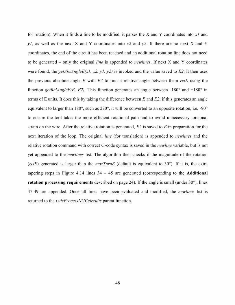
48
for rotation). When it finds a line to be modified, it parses the X and Y coordinates into x1 and
y1, as well as the next X and Y coordinates into x2 and y2. If there are no next X and Y
coordinates, the end of the circuit has been reached and an additional rotation line does not need
to be generated – only the original line is appended to newlines. If next X and Y coordinates
were found, the getAbsAngleE(x1, x2, y1, y2) is invoked and the value saved to E2. It then uses
the previous absolute angle E with E2 to find a relative angle between them relE using the
function getRelAngleE(E, E2). This function generates an angle between -180° and +180° in
terms of E units. It does this by taking the difference between E and E2; if this generates an angle
equivalent to larger than 180°, such as 270°, it will be converted to an opposite rotation, i.e. -90°
to ensure the tool takes the more efficient rotational path and to avoid unnecessary torsional
strain on the wire. After the relative rotation is generated, E2 is saved to E in preparation for the
next iteration of the loop. The original line (for translation) is appended to newlines and the
relative rotation command with correct G-code syntax is saved in the newline variable, but is not
yet appended to the newlines list. The algorithm then checks if the magnitude of the rotation
(relE) generated is larger than the maxTurnE (default is equivalent to 30°). If it is, the extra
tapering steps in Figure 4.14 lines 34 – 45 are generated (corresponding to the Additional
rotation processing requirements described on page 24). If the angle is small (under 30°), lines
47-49 are appended. Once all lines have been evaluated and modified, the newlines list is
returned to the LulzProcessNGCcircuits parent function.
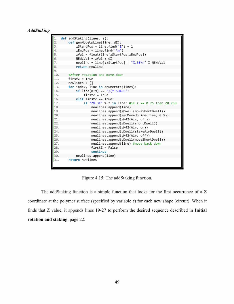
49
AddStaking
1. def addStaking(lines, z): 2. def genMoveUpLine(line, dZ): 3. zStartPos = line.find('Z') + 1 4. zEndPos = line.find('\n') 5. zVal = float(line[zStartPos:zEndPos]) 6. NEWzVal = zVal + dZ 7. newline = line[:zStartPos] + "%.3f\n" % NEWzVal 8. return newline 9. 10. #After rotation and move down 11. firstZ = True 12. newlines = [] 13. for index, line in enumerate(lines): 14. if line[0:9] == ";(* SHAPE": 15. firstZ = True 16. elif firstZ == True: 17. if "Z%.3f" % z in line: #if z == 0.75 then Z0.750 18. newlines.append(line) 19. newlines.append(gDwell(moveShortDwell)) 20. newlines.append(genMoveUpLine(line, 0.5)) 21. newlines.append(gM42(Air, off)) 22. newlines.append(gDwell(shortDwell)) 23. newlines.append(gM42(Air, on)) 24. newlines.append(gDwell(stakeAirDwell)) 25. newlines.append(gM42(Air, off)) 26. newlines.append(gDwell(moveShortDwell)) 27. newlines.append(line) #move back down 28. firstZ = False 29. continue 30. newlines.append(line) 31. return newlines
Figure 4.15: The addStaking function.
The addStaking function is a simple function that looks for the first occurrence of a Z
coordinate at the polymer surface (specified by variable z) for each new shape (circuit). When it
finds that Z value, it appends lines 19-27 to perform the desired sequence described in Initial
rotation and staking, page 22.
50
AddCutting
1. def addCutting(lines, taperDistance, taperTheta, z1, taperF, moveDistance, moveTheta, moveF, strokes):
2. 3. def genEndCoolingLines(): 4. coolingLines = [] 5. coolingLines.append(gM42(Air, off)) 6. coolingLines.append(gDwell(shortDwell)) 7. coolingLines.append(gM42(Air, on)) 8. coolingLines.append(gDwell(coolDwell)) 9. coolingLines.append(gM42(Air, off)) 10. return coolingLines 11. 12. newlines = [] 13. for index, line in enumerate(lines): 14. 15. if ((line[0:2] == "G1") and ("Z%.3f" % (z1 + 3) in line)): #replace verticle Z mov
ement with taper, cool, move, and cut. 16. 17. #get the xy plane vector (used to get the direction for taper and move) 18. dx, dy, x1, y1 = getDXDYx1y1(lines, index - 1) 19. 20. #taper 21. comment = "tool taper added by Python/genTaperLine" 22. taperLine, x2, y2, z2 = genTaperLineX2Y2Z2(taperDistance, taperTheta, x1, y1,
z1, dx, dy, taperF, comment) 23. newlines.append(taperLine) 24. 25. #cool 26. coolingLines = genEndCoolingLines() 27. for line in coolingLines: 28. newlines.append(line) 29. 30. #move and dwell 31. comment = "tool move added by Python/genTaperLine" 32. moveLine, x2, y2, z2 = genTaperLineX2Y2Z2(moveDistance, moveTheta, x2, y2, z2,
dx, dy, moveF, comment) #to generate the move line, we use the taper function with a theta of 0 degrees.
33. newlines.append(moveLine) 34. newlines.append(gDwell(moveDwell)) 35. 36. #cut 37. j = 1 38. 39. newlines.append(gM42(Cutter, off)) 40. newlines.append(gDwell(shortDwell)) 41. while j <= strokes: 42. newlines.append(gM42(Cutter, on)) 43. newlines.append(gDwell(shortDwell)) 44. newlines.append(gM42(Cutter, off)) 45. newlines.append(gDwell(shortDwell)) 46. j += 1 47. else: 48. newlines.append(line) 49. return newlines
Figure 4.16: The addCutting function.
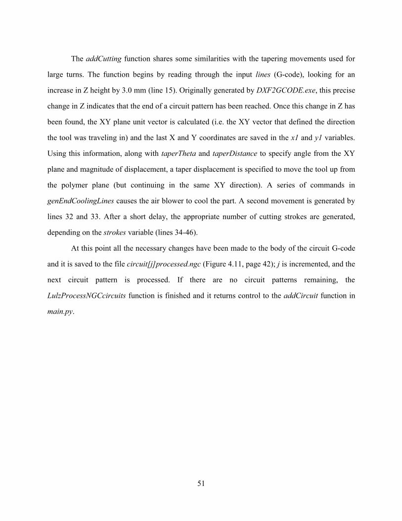
51
The addCutting function shares some similarities with the tapering movements used for
large turns. The function begins by reading through the input lines (G-code), looking for an
increase in Z height by 3.0 mm (line 15). Originally generated by DXF2GCODE.exe, this precise
change in Z indicates that the end of a circuit pattern has been reached. Once this change in Z has
been found, the XY plane unit vector is calculated (i.e. the XY vector that defined the direction
the tool was traveling in) and the last X and Y coordinates are saved in the x1 and y1 variables.
Using this information, along with taperTheta and taperDistance to specify angle from the XY
plane and magnitude of displacement, a taper displacement is specified to move the tool up from
the polymer plane (but continuing in the same XY direction). A series of commands in
genEndCoolingLines causes the air blower to cool the part. A second movement is generated by
lines 32 and 33. After a short delay, the appropriate number of cutting strokes are generated,
depending on the strokes variable (lines 34-46).
At this point all the necessary changes have been made to the body of the circuit G-code
and it is saved to the file circuit[j]processed.ngc (Figure 4.11, page 42); j is incremented, and the
next circuit pattern is processed. If there are no circuit patterns remaining, the
LulzProcessNGCcircuits function is finished and it returns control to the addCircuit function in
main.py.
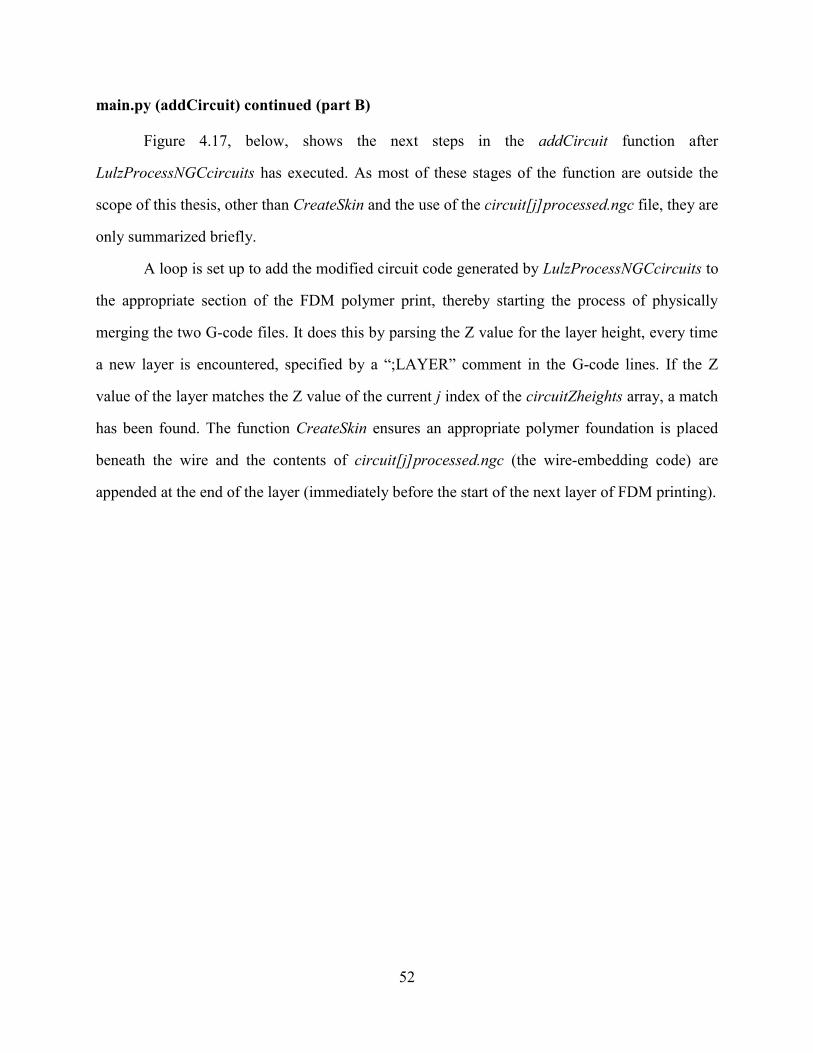
52
main.py (addCircuit) continued (part B)
Figure 4.17, below, shows the next steps in the addCircuit function after
LulzProcessNGCcircuits has executed. As most of these stages of the function are outside the
scope of this thesis, other than CreateSkin and the use of the circuit[j]processed.ngc file, they are
only summarized briefly.
A loop is set up to add the modified circuit code generated by LulzProcessNGCcircuits to
the appropriate section of the FDM polymer print, thereby starting the process of physically
merging the two G-code files. It does this by parsing the Z value for the layer height, every time
a new layer is encountered, specified by a “;LAYER” comment in the G-code lines. If the Z
value of the layer matches the Z value of the current j index of the circuitZheights array, a match
has been found. The function CreateSkin ensures an appropriate polymer foundation is placed
beneath the wire and the contents of circuit[j]processed.ngc (the wire-embedding code) are
appended at the end of the layer (immediately before the start of the next layer of FDM printing).
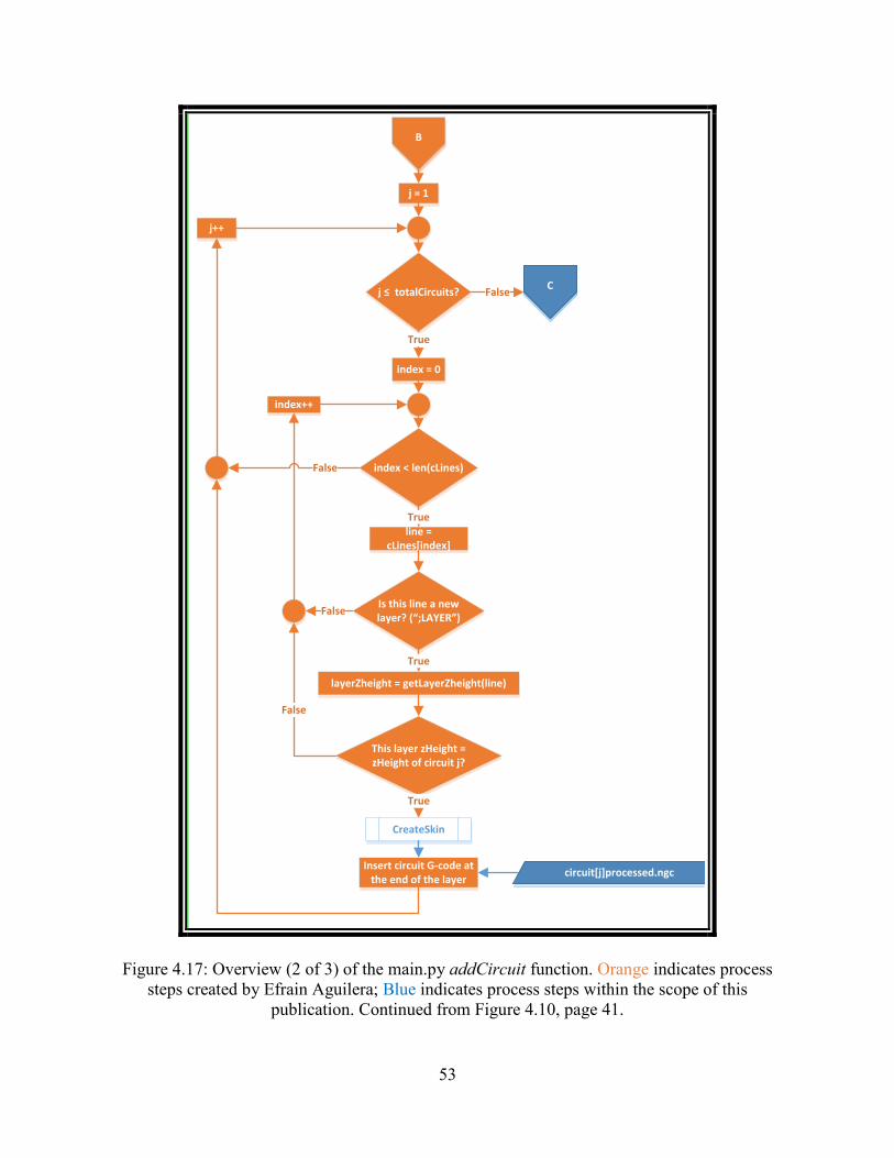
53
BB
j � totalCircuits?
j = 1
This layer zHeight = zHeight of circuit j?
index = 0
index < len(cLines)
Is this line a new layer? LAYER
line = cLines[index]
True
layerZheight = getLayerZheight(line)
True
True
CC
index++
False
False
CreateSkin
Insert circuit G-code at the end of the layer
circuit[j]processed.ngc
True
False
j++
False
Figure 4.17: Overview (2 of 3) of the main.py addCircuit function. Orange indicates process
steps created by Efrain Aguilera; Blue indicates process steps within the scope of this
publication. Continued from Figure 4.10, page 41.
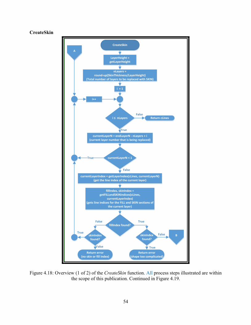
54
CreateSkin
CreateSkin
i � nLayers
currentLayerN = endLayerN - nLayers + i(current layer number that is being replaced)
Return cLinesFalse
True
i++
LayerHeight = getLayerHeight
fillIndex found?
nLayers = round-up(SkinThickness/LayerHeight)
(Total number of layers to be replaced with SKIN)
i = 1
currentLayerN < 1True
currentLayerIndex = getLayerIndex(cLines, currentLayerN)(get the line index of the current layer)
False
fillIndex, skinIndex = getFILLandSKINindices(cLines,
currentLayerIndex)(gets line indices for the FILL and SKIN sections of
the current layer)
skinIndex found?
Return error (no skin or fill index)
False
False
TrueskinIndex
found?
True
Return error (shape too complicated)
True
BBFalse
AA
Figure 4.18: Overview (1 of 2) of the CreateSkin function. All process steps illustrated are within
the scope of this publication. Continued in Figure 4.19.
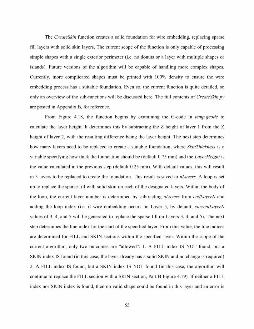
55
The CreateSkin function creates a solid foundation for wire embedding, replacing sparse
fill layers with solid skin layers. The current scope of the function is only capable of processing
simple shapes with a single exterior perimeter (i.e. no donuts or a layer with multiple shapes or
islands). Future versions of the algorithm will be capable of handling more complex shapes.
Currently, more complicated shapes must be printed with 100% density to ensure the wire
embedding process has a suitable foundation. Even so, the current function is quite detailed, so
only an overview of the sub-functions will be discussed here. The full contents of CreateSkin.py
are posted in Appendix B, for reference.
From Figure 4.18, the function begins by examining the G-code in temp.gcode to
calculate the layer height. It determines this by subtracting the Z height of layer 1 from the Z
height of layer 2, with the resulting difference being the layer height. The next step determines
how many layers need to be replaced to create a suitable foundation, where SkinThickness is a
variable specifying how thick the foundation should be (default 0.75 mm) and the LayerHeight is
the value calculated in the previous step (default 0.25 mm). With default values, this will result
in 3 layers to be replaced to create the foundation. This result is saved to nLayers. A loop is set
up to replace the sparse fill with solid skin on each of the designated layers. Within the body of
the loop, the current layer number is determined by subtracting nLayers from endLayerN and
adding the loop index (i.e. if wire embedding occurs on Layer 5, by default, currentLayerN
values of 3, 4, and 5 will be generated to replace the sparse fill on Layers 3, 4, and 5). The next
step determines the line index for the start of the specified layer. From this value, the line indices
are determined for FILL and SKIN sections within the specified layer. Within the scope of the
current algorithm, only two outcomes are “allowed”: 1. A FILL index IS NOT found, but a
SKIN index IS found (in this case, the layer already has a solid SKIN and no change is required)
2. A FILL index IS found, but a SKIN index IS NOT found (in this case, the algorithm will
continue to replace the FILL section with a SKIN section, Part B Figure 4.19). If neither a FILL
index nor SKIN index is found, then no valid shape could be found in this layer and an error is
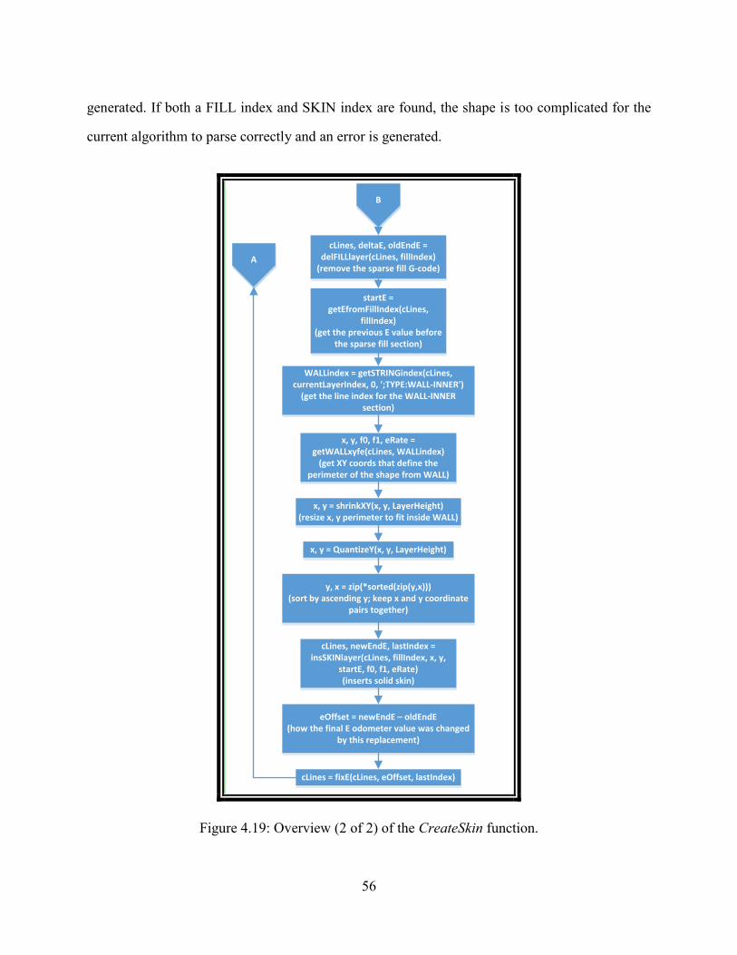
56
generated. If both a FILL index and SKIN index are found, the shape is too complicated for the
current algorithm to parse correctly and an error is generated.
BB
cLines, deltaE, oldEndE = delFILLlayer(cLines, fillIndex)
(remove the sparse fill G-code)
startE = getEfromFillIndex(cLines,
fillIndex)(get the previous E value before
the sparse fill section)
WALLindex = getSTRINGindex(cLines, currentLayerIndex, 0, ';TYPE:WALL-INNER')
(get the line index for the WALL-INNER section)
x, y, f0, f1, eRate = getWALLxyfe(cLines, WALLindex)
(get XY coords that define the perimeter of the shape from WALL)
x, y = shrinkXY(x, y, LayerHeight)(resize x, y perimeter to fit inside WALL)
x, y = QuantizeY(x, y, LayerHeight)
y, x = zip(*sorted(zip(y,x))) (sort by ascending y; keep x and y coordinate
pairs together)
cLines, newEndE, lastIndex = insSKINlayer(cLines, fillIndex, x, y,
startE, f0, f1, eRate)(inserts solid skin)
eOffset = newEndE – oldEndE(how the final E odometer value was changed
by this replacement)
cLines = fixE(cLines, eOffset, lastIndex)
AA
Figure 4.19: Overview (2 of 2) of the CreateSkin function.
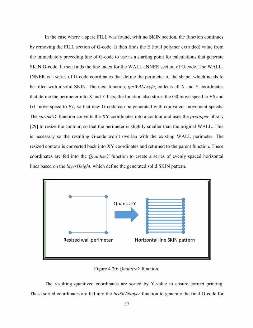
57
In the case where a spare FILL was found, with no SKIN section, the function continues
by removing the FILL section of G-code. It then finds the E (total polymer extruded) value from
the immediately preceding line of G-code to use as a starting point for calculations that generate
SKIN G-code. It then finds the line index for the WALL-INNER section of G-code. The WALL-
INNER is a series of G-code coordinates that define the perimeter of the shape, which needs to
be filled with a solid SKIN. The next function, getWALLxyfe, collects all X and Y coordinates
that define the perimeter into X and Y lists; the function also stores the G0 move speed to F0 and
G1 move speed to F1, so that new G-code can be generated with equivalent movement speeds.
The shrinkXY function converts the XY coordinates into a contour and uses the pyclipper library
[29] to resize the contour, so that the perimeter is slightly smaller than the original WALL. This
is necessary so the resulting G-code won’t overlap with the existing WALL perimeter. The
resized contour is converted back into XY coordinates and returned to the parent function. These
coordinates are fed into the QuantizeY function to create a series of evenly spaced horizontal
lines based on the layerHeight, which define the generated solid SKIN pattern.
Figure 4.20: QuantizeY function.
The resulting quantized coordinates are sorted by Y-value to ensure correct printing.
These sorted coordinates are fed into the insSKINlayer function to generate the final G-code for
58
the SKIN section with the correct syntax. Finally, the remainder of the G-code has to be fixed to
account for the changes to the E extrusion value. The old value for E at the end of the deleted
sparse FILL section is compared to the new value for E at the end of the added solid SKIN
section. The difference between new and old E is added to all subsequent E values by the fixE
function to ensure correct printing. The loop then continues until all necessary sparse FILL
layers have been replaced by solid SKIN. With the foundation modified, control is passed back
to addCircuit in main.py, Figure 4.17 page 53, which proceeds by inserting the circuit pattern G-
code before continuing on to part C below.
main.py (addCircuit) continued (part C)
CC
Apply FDM Z Offset
Is generated G-code within build area?
Have all circuits have been inserted?
Error: Generate error message
False
False
True
FileSlicer(cLines, filePath)
finalOutput.gcodePart 1 –�Polymer.gcode
Part 2 Circuit.gcode...
Success: Generate success message
return
Figure 4.21: Overview (3 of 3) of the main.py addCircuit function. All process steps illustrated
are within the scope of this publication. Continued from Figure 4.17, page 53.
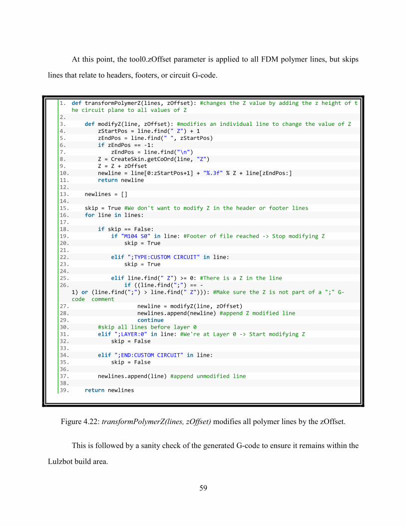
59
At this point, the tool0.zOffset parameter is applied to all FDM polymer lines, but skips
lines that relate to headers, footers, or circuit G-code.
1. def transformPolymerZ(lines, zOffset): #changes the Z value by adding the z height of the circuit plane to all values of Z
2. 3. def modifyZ(line, zOffset): #modifies an individual line to change the value of Z 4. zStartPos = line.find(" Z") + 1 5. zEndPos = line.find(" ", zStartPos) 6. if zEndPos == -1: 7. zEndPos = line.find("\n") 8. Z = CreateSkin.getCoOrd(line, "Z") 9. Z = Z + zOffset 10. newline = line[0:zStartPos+1] + "%.3f" % Z + line[zEndPos:] 11. return newline 12. 13. newlines = [] 14. 15. skip = True #We don't want to modify Z in the header or footer lines 16. for line in lines: 17. 18. if skip == False: 19. if "M104 S0" in line: #Footer of file reached -> Stop modifying Z 20. skip = True 21. 22. elif ";TYPE:CUSTOM CIRCUIT" in line: 23. skip = True 24. 25. elif line.find(" Z") >= 0: #There is a Z in the line 26. if ((line.find(";") == -
1) or (line.find(";") > line.find(" Z"))): #Make sure the Z is not part of a ";" G-code comment
27. newline = modifyZ(line, zOffset) 28. newlines.append(newline) #append Z modified line 29. continue 30. #skip all lines before layer 0 31. elif ";LAYER:0" in line: #We're at Layer 0 -> Start modifying Z 32. skip = False 33. 34. elif ";END:CUSTOM CIRCUIT" in line: 35. skip = False 36. 37. newlines.append(line) #append unmodified line 38. 39. return newlines
Figure 4.22: transformPolymerZ(lines, zOffset) modifies all polymer lines by the zOffset.
This is followed by a sanity check of the generated G-code to ensure it remains within the
Lulzbot build area.
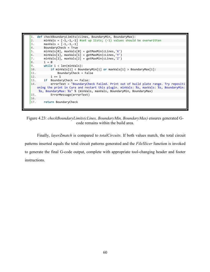
60
1. def checkBoundaryLimits(cLines, BoundaryMin, BoundaryMax): 2. minVals = [-1,-1,-1] #set up lists; (-1) values should be overwritten 3. maxVals = [-1,-1,-1] 4. BoundaryCheck = True 5. minVals[0], maxVals[0] = getMaxMin(cLines,'X') 6. minVals[1], maxVals[1] = getMaxMin(cLines,'Y') 7. minVals[2], maxVals[2] = getMaxMin(cLines,'Z') 8. i = 0 9. while i < len(minVals): 10. if minVals[i] < BoundaryMin[i] or maxVals[i] > BoundaryMax[i]: 11. BoundaryCheck = False 12. i += 1 13. if BoundaryCheck == False: 14. errorText = "BoundaryCheck Failed. Print out of build plate range. Try repositi
oning the print in Cura and restart this plugin. minVals: %s, maxVals: %s, BoundaryMin: %s, BoundaryMax: %s" % (minVals, maxVals, BoundaryMin, BoundaryMax)
15. ErrorMessage(errorText) 16. 17. return BoundaryCheck
Figure 4.23: checkBoundaryLimits(cLines, BoundaryMin, BoundaryMax) ensures generated G-
code remains within the build area.
Finally, layerZmatch is compared to totalCircuits. If both values match, the total circuit
patterns inserted equals the total circuit patterns generated and the FileSlicer function is invoked
to generate the final G-code output, complete with appropriate tool-changing header and footer
instructions.
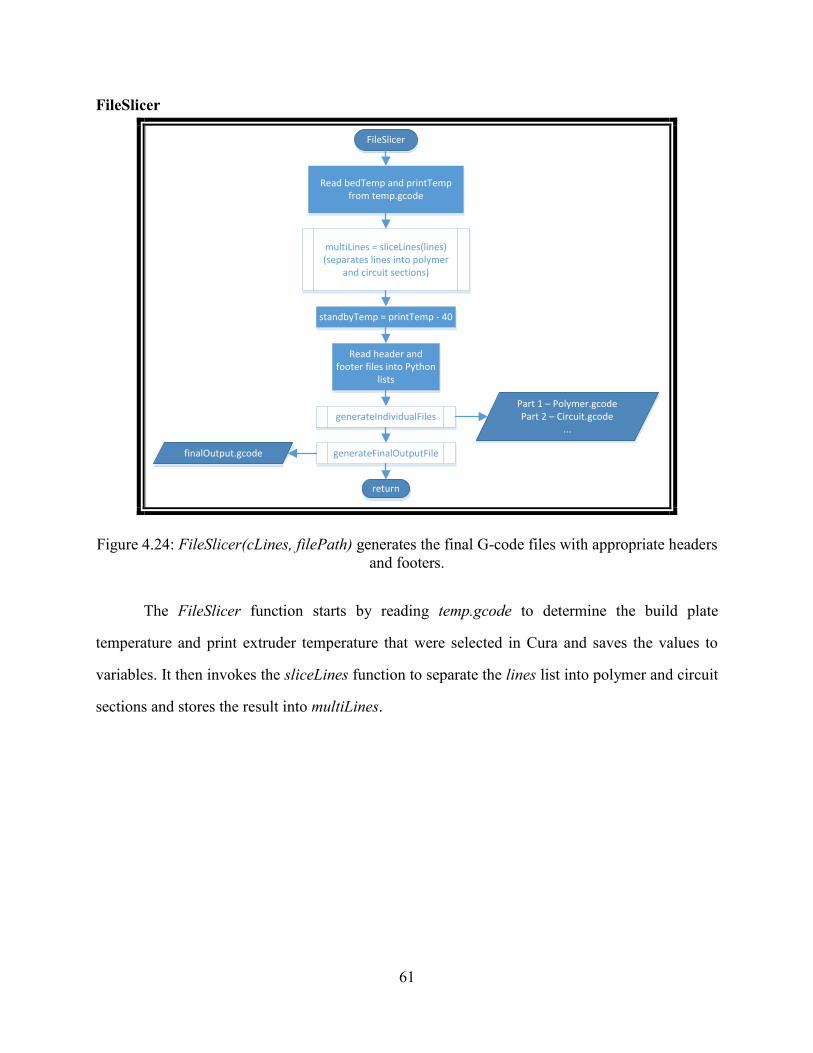
61
FileSlicer
FileSlicer
Read bedTemp and printTemp from temp.gcode
multiLines = sliceLines(lines)(separates lines into polymer
and circuit sections)
standbyTemp = printTemp - 40
Read header and footer files into Python
lists
generateIndividualFiles
generateFinalOutputFile
return
finalOutput.gcode
Part 1 –�Polymer.gcodePart 2 –�Circuit.gcode
...
Figure 4.24: FileSlicer(cLines, filePath) generates the final G-code files with appropriate headers
and footers.
The FileSlicer function starts by reading temp.gcode to determine the build plate
temperature and print extruder temperature that were selected in Cura and saves the values to
variables. It then invokes the sliceLines function to separate the lines list into polymer and circuit
sections and stores the result into multiLines.
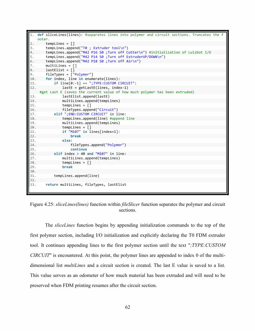
62
1. def sliceLines(lines): #separates lines into polymer and circuit sections. Truncates the footer.
2. tempLines = [] 3. tempLines.append("T0 ; Extruder tool\n") 4. tempLines.append("M42 P16 S0 ;Turn off Cutter\n") #initialization of Lulzbot I/O 5. tempLines.append("M42 P14 S0 ;Turn off ExtruderUP/DOWN\n") 6. tempLines.append("M42 P18 S0 ;Turn off Air\n") 7. multiLines = [] 8. lastElist = [] 9. fileTypes = ["Polymer"] 10. for index, line in enumerate(lines): 11. if line[0:-1] == ";TYPE:CUSTOM CIRCUIT": 12. lastE = getLastE(lines, index-1)
#get Last E (saves the current value of how much polymer has been extruded) 13. lastElist.append(lastE) 14. multiLines.append(tempLines) 15. tempLines = [] 16. fileTypes.append("Circuit") 17. elif ";END:CUSTOM CIRCUIT" in line: 18. tempLines.append(line) #append line 19. multiLines.append(tempLines) 20. tempLines = [] 21. if "M107" in lines[index+1]: 22. break 23. else: 24. fileTypes.append("Polymer") 25. continue 26. elif index > 40 and "M107" in line: 27. multiLines.append(tempLines) 28. tempLines = [] 29. break 30. 31. tempLines.append(line) 32. 33. return multiLines, fileTypes, lastElist
Figure 4.25: sliceLines(lines) function within fileSlicer function separates the polymer and circuit
sections.
The sliceLines function begins by appending initialization commands to the top of the
first polymer section, including I/O initialization and explicitly declaring the T0 FDM extruder
tool. It continues appending lines to the first polymer section until the text ";TYPE:CUSTOM
CIRCUIT" is encountered. At this point, the polymer lines are appended to index 0 of the multi-
dimensional list multiLines and a circuit section is created. The last E value is saved to a list.
This value serves as an odometer of how much material has been extruded and will need to be
preserved when FDM printing resumes after the circuit section.
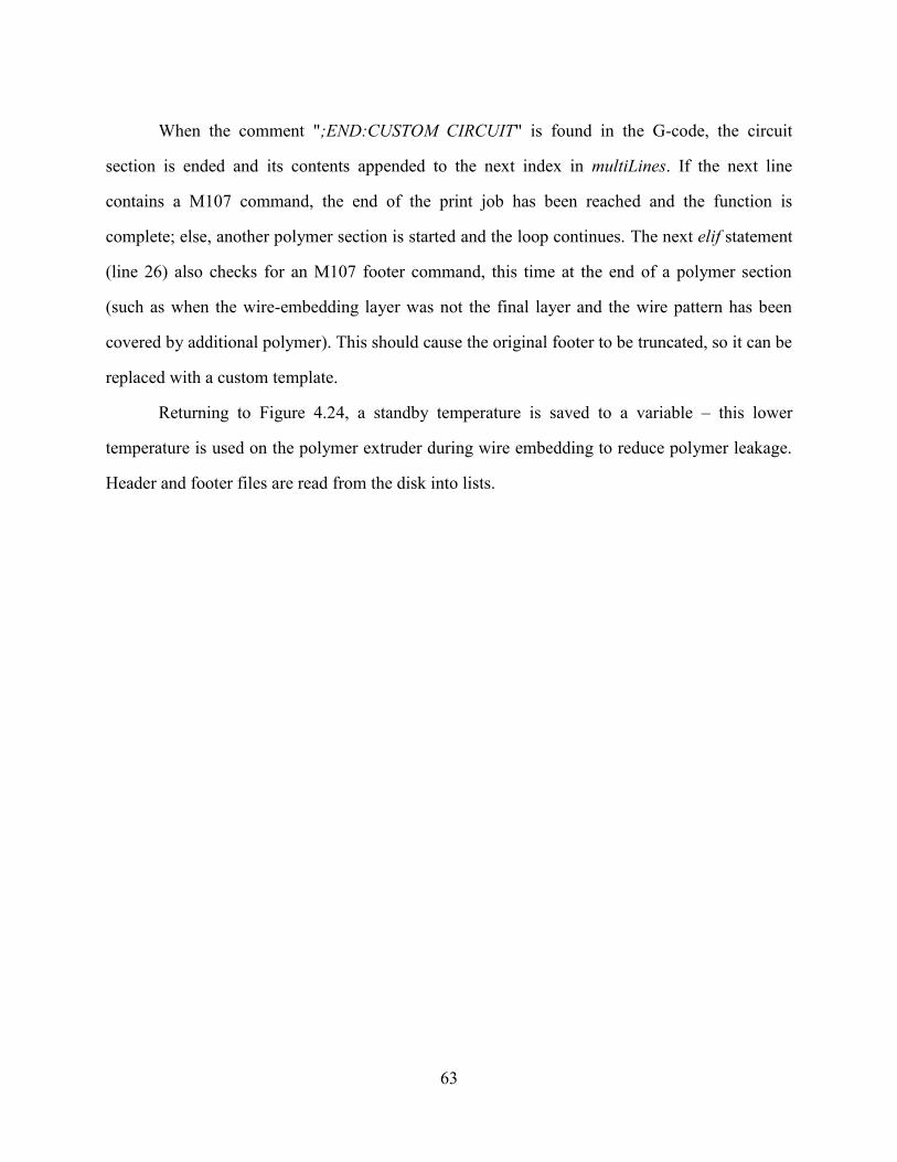
63
When the comment ";END:CUSTOM CIRCUIT" is found in the G-code, the circuit
section is ended and its contents appended to the next index in multiLines. If the next line
contains a M107 command, the end of the print job has been reached and the function is
complete; else, another polymer section is started and the loop continues. The next elif statement
(line 26) also checks for an M107 footer command, this time at the end of a polymer section
(such as when the wire-embedding layer was not the final layer and the wire pattern has been
covered by additional polymer). This should cause the original footer to be truncated, so it can be
replaced with a custom template.
Returning to Figure 4.24, a standby temperature is saved to a variable – this lower
temperature is used on the polymer extruder during wire embedding to reduce polymer leakage.
Header and footer files are read from the disk into lists.
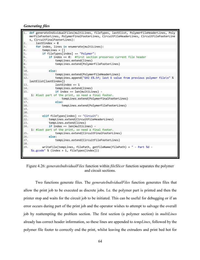
64
Generating files
1. def generateIndividualFiles(multiLines, fileTypes, lastElist, PolymerFileHeaderLines, PolymerFileFooterLines, PolymerFinalFooterLines, CircuitFileHeaderLines, CircuitFileFooterLines, CircuitFinalFooterLines):
2. lastEindex = 0 3. for index, lines in enumerate(multiLines): 4. tempLines = [] 5. if fileTypes[index] == "Polymer": 6. if index == 0: #first section preserves current file header 7. tempLines.extend(lines) 8. tempLines.extend(PolymerFileFooterLines) 9. 10. else: 11. tempLines.extend(PolymerFileHeaderLines) 12. tempLines.append("G92 E%.5f; last E value from previous polymer file\n" %
lastElist[lastEindex]) 13. lastEindex += 1 14. tempLines.extend(lines) 15. if index == len(multiLines) -
1: #last part of the print, so need a final footer. 16. tempLines.extend(PolymerFinalFooterLines) 17. else: 18. tempLines.extend(PolymerFileFooterLines) 19. 20. 21. elif fileTypes[index] == "Circuit": 22. tempLines.extend(CircuitFileHeaderLines) 23. tempLines.extend(lines) 24. if index == len(multiLines) -
1: #last part of the print, so need a final footer. 25. tempLines.extend(CircuitFinalFooterLines) 26. else: 27. tempLines.extend(CircuitFileFooterLines) 28. 29. writeFile(tempLines, filePath, getFileName(filePath) + " - Part %d -
%s.gcode" % (index + 1, fileTypes[index]))
Figure 4.26: generateIndividualFiles function within fileSlicer function separates the polymer
and circuit sections.
Two functions generate files. The generateIndividualFiles function generates files that
allow the print job to be executed as discrete jobs. I.e. the polymer part is printed and then the
printer stop and waits for the circuit job to be initiated. This can be useful for debugging or if an
error occurs during part of the print job and the operator wishes to attempt to salvage the overall
job by reattempting the problem section. The first section (a polymer section) in multiLines
already has correct header information, so these lines are appended to tempLines, followed by the
polymer file footer to correctly end the print, whilst leaving the extruders and print bed hot for
65
the next job. The tempLines are written to “Filename” – 1 – Polymer.gcode. Subsequent
polymer sections are handled by lines 10 – 18. These sections require a header to be appended to
the top to correctly initialize the print, as well as a G92 command with the last E value to
correctly “rezero” the extrusion odometer (if this wasn’t added, the first print command would
cause a very large amount of material to be extruded, equal to the amount used in the earlier
parts of the print job). The next if statement checks whether this was the final part of the print to
determine which footer to use – i.e. should all heaters be turned off? The circuit sections are
handled in a similar manner, except no special treatment is needed for the first circuit section.
The single file output function, generateFinalOutputFile, has a similar algorithm, albeit with
slightly different intermediate footers and with all outputs appended to the same list and
ultimately the same file (Figure 4.27).
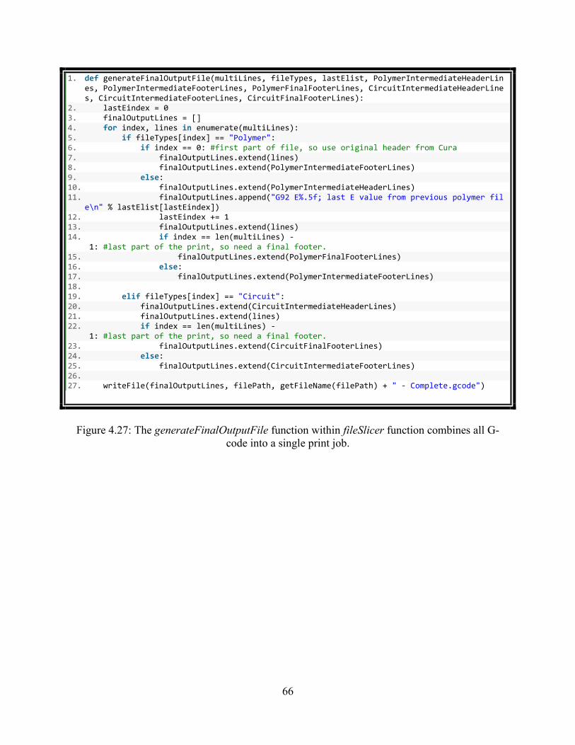
66
1. def generateFinalOutputFile(multiLines, fileTypes, lastElist, PolymerIntermediateHeaderLines, PolymerIntermediateFooterLines, PolymerFinalFooterLines, CircuitIntermediateHeaderLines, CircuitIntermediateFooterLines, CircuitFinalFooterLines):
2. lastEindex = 0 3. finalOutputLines = [] 4. for index, lines in enumerate(multiLines): 5. if fileTypes[index] == "Polymer": 6. if index == 0: #first part of file, so use original header from Cura 7. finalOutputLines.extend(lines) 8. finalOutputLines.extend(PolymerIntermediateFooterLines) 9. else: 10. finalOutputLines.extend(PolymerIntermediateHeaderLines) 11. finalOutputLines.append("G92 E%.5f; last E value from previous polymer fil
e\n" % lastElist[lastEindex]) 12. lastEindex += 1 13. finalOutputLines.extend(lines) 14. if index == len(multiLines) -
1: #last part of the print, so need a final footer. 15. finalOutputLines.extend(PolymerFinalFooterLines) 16. else: 17. finalOutputLines.extend(PolymerIntermediateFooterLines) 18. 19. elif fileTypes[index] == "Circuit": 20. finalOutputLines.extend(CircuitIntermediateHeaderLines) 21. finalOutputLines.extend(lines) 22. if index == len(multiLines) -
1: #last part of the print, so need a final footer. 23. finalOutputLines.extend(CircuitFinalFooterLines) 24. else: 25. finalOutputLines.extend(CircuitIntermediateFooterLines) 26. 27. writeFile(finalOutputLines, filePath, getFileName(filePath) + " - Complete.gcode")
Figure 4.27: The generateFinalOutputFile function within fileSlicer function combines all G-
code into a single print job.
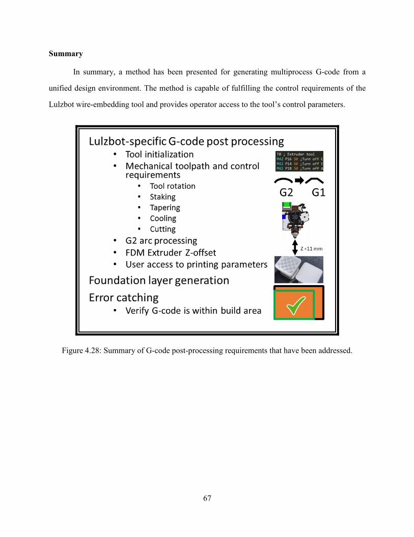
67
Summary
In summary, a method has been presented for generating multiprocess G-code from a
unified design environment. The method is capable of fulfilling the control requirements of the
Lulzbot wire-embedding tool and provides operator access to the tool’s control parameters.
Figure 4.28: Summary of G-code post-processing requirements that have been addressed.
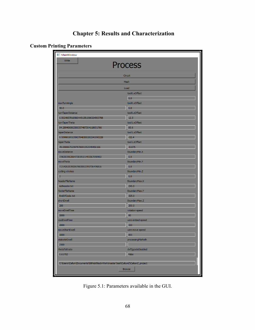
68
Chapter 5: Results and Characterization
Custom Printing Parameters
Figure 5.1: Parameters available in the GUI.
69
The GUI provides parameter access to the printer operator. Figure 5.1 shows the layout of
the GUI and default parameter values. The first three parameters relate to basic control of tool
orientation: maxTurnAngle corresponds to the maximum angle the wire-embedding head can
turn in degrees, before it needs to be raised for additional processing steps (as described in
Chapter 3). turnTaperDistance and turnTaperTheta are parameters for the additional processing
steps for a turn greater than maxTurnAngle. The next five parameters relate to the cutting
algorithm: taperDistance and taperTheta specify the displacement vector (magnitude and angle
from the polymer plane) that the tool should take after reaching its last point before a cut. Then
moveDistance and moveTheta specify an additional displacement vector before the cut, while
cutting-strokes specifies the number of times the cutting actuator should activate for each cut.
These parameters are followed by a number of Dwell parameters, which specify delay times in
ms between various commands. The thetaToEratio is a radians-to-E-rotation value conversion
used by the addToolRotation function (1 radian corresponds to 0.61752; 2π radians corresponds
to 3.88); this value can be adjusted to larger values if the tool is not rotating sufficiently for a
given angle and vice versa. A number of x, y, and z offsets are specified, with tool0
corresponding to the FDM extruder and tool1 corresponding to the wire-embedding tool. The
BoundaryMax parameters specify the minimum and maximum dimensions of the build area;
these parameters are compared with the G-code coordinates generated to ensure the print job is
contained within the build area. The parameters rotation-speed, wire-embed-speed, and wire-
move-speed specify the “F” value (speed) to be used when generating G-code lines for wire-
embedding head tool rotation, embedding wire in polymer, and moving between wire-embedding
coordinates. Of the last two parameters, processingFilePath is defunct and will be removed in a
future version of the GUI, whereas dxf2gcodeDisabled is a special parameter, that when set to
True will disable the DXF2GCODE.exe functionality of the program. The purpose of this is to
allow the user the option to open the DXF2GCODE.exe GUI and specify specific parameters for
creating the basic G-code file instead of the standard parameters used by the Python program.
The most common current use for this feature is to reverse the direction of the G-code generated
70
by DXF2GCODE.exe; e.g. if the script generated wire-embedding G-code for a spiral with the
embedding starting at the center of the spiral and ending on the outside, the user could reverse
this direction by disabling DXF2GCODE and manually reversing the direction of the G-code
generation (see Figure 5.13, page 82, for an example). In future versions of the GUI, it is planned
to introduce a feature that will allow this tool reversal to be implemented automatically from the
wire-embedding GUI.
Testing
For the purposes of evaluating the successfulness of this software solution, a number of
test print jobs have been generated. The following print functions (and their tunable parameters)
will be tested: Staking (tool1.zOffset, moveShortDwell, shortDwell, stakeAirDwell), straight
lines (wire-embed-speed, tool1.[x,y,z]Offset), small turns (maxTurnAngle, thetaToEratio,
rotation-speed), large turns (maxTurnAngle, turnTaperDistance, turnTaperTheta,
thetaToEratio, shortDwell, moveDwell. moveShortDwell, rotation-speed), cutting
(taperDistance, taperTheta, moveDistance, moveTheta, cutting-strokes, shortDwell.
moveDwellTime, coolDwellTime), G2 conversion (maxArcLength [not in GUI], macArcTheta
[not in GUI]), and the CreateSkin function.
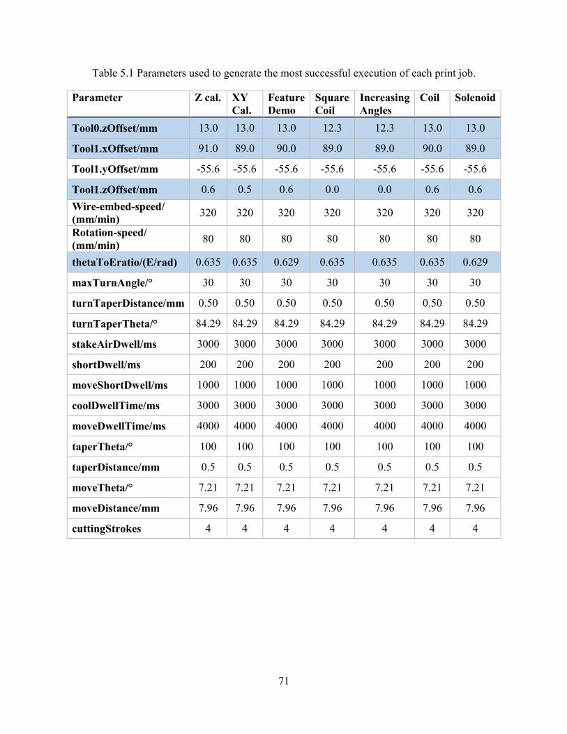
71
Table 5.1 Parameters used to generate the most successful execution of each print job.
Parameter Z cal. XY
Cal.
Feature
Demo
Square
Coil
Increasing
Angles
Coil Solenoid
Tool0.zOffset/mm 13.0 13.0 13.0 12.3 12.3 13.0 13.0
Tool1.xOffset/mm 91.0 89.0 90.0 89.0 89.0 90.0 89.0
Tool1.yOffset/mm -55.6 -55.6 -55.6 -55.6 -55.6 -55.6 -55.6
Tool1.zOffset/mm 0.6 0.5 0.6 0.0 0.0 0.6 0.6
Wire-embed-speed/
(mm/min) 320 320 320 320 320 320 320
Rotation-speed/
(mm/min) 80 80 80 80 80 80 80
thetaToEratio/(E/rad) 0.635 0.635 0.629 0.635 0.635 0.635 0.629
maxTurnAngle/° 30 30 30 30 30 30 30
turnTaperDistance/mm 0.50 0.50 0.50 0.50 0.50 0.50 0.50
turnTaperTheta/° 84.29 84.29 84.29 84.29 84.29 84.29 84.29
stakeAirDwell/ms 3000 3000 3000 3000 3000 3000 3000
shortDwell/ms 200 200 200 200 200 200 200
moveShortDwell/ms 1000 1000 1000 1000 1000 1000 1000
coolDwellTime/ms 3000 3000 3000 3000 3000 3000 3000
moveDwellTime/ms 4000 4000 4000 4000 4000 4000 4000
taperTheta/° 100 100 100 100 100 100 100
taperDistance/mm 0.5 0.5 0.5 0.5 0.5 0.5 0.5
moveTheta/° 7.21 7.21 7.21 7.21 7.21 7.21 7.21
moveDistance/mm 7.96 7.96 7.96 7.96 7.96 7.96 7.96
cuttingStrokes 4 4 4 4 4 4 4
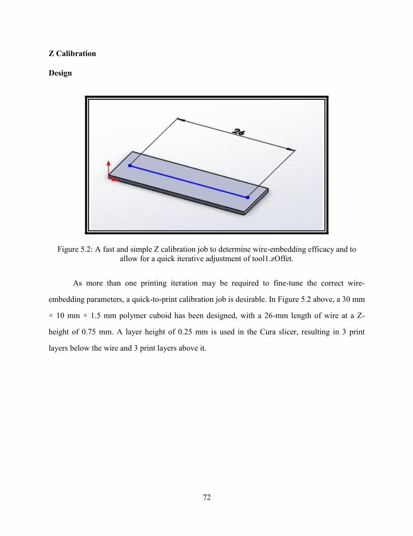
72
Z Calibration
Design
Figure 5.2: A fast and simple Z calibration job to determine wire-embedding efficacy and to
allow for a quick iterative adjustment of tool1.zOffet.
As more than one printing iteration may be required to fine-tune the correct wire-
embedding parameters, a quick-to-print calibration job is desirable. In Figure 5.2 above, a 30 mm
× 10 mm × 1.5 mm polymer cuboid has been designed, with a 26-mm length of wire at a Z-
height of 0.75 mm. A layer height of 0.25 mm is used in the Cura slicer, resulting in 3 print
layers below the wire and 3 print layers above it.
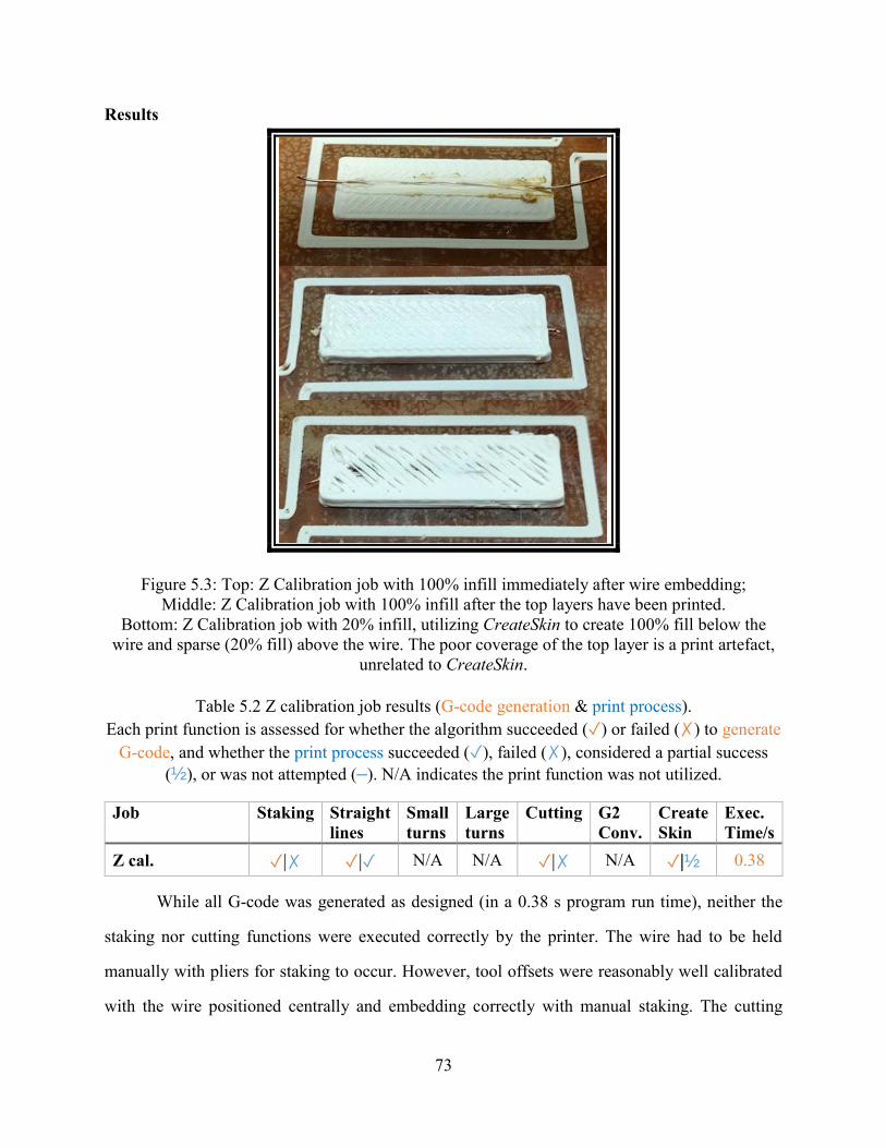
73
Results
Figure 5.3: Top: Z Calibration job with 100% infill immediately after wire embedding;
Middle: Z Calibration job with 100% infill after the top layers have been printed.
Bottom: Z Calibration job with 20% infill, utilizing CreateSkin to create 100% fill below the
wire and sparse (20% fill) above the wire. The poor coverage of the top layer is a print artefact,
unrelated to CreateSkin.
Table 5.2 Z calibration job results (G-code generation & print process).
Each print function is assessed for whether the algorithm succeeded (✓) or failed (✗) to generate
G-code, and whether the print process succeeded (✓), failed (✗), considered a partial success
(½), or was not attempted (–). N/A indicates the print function was not utilized.
Job Staking Straight
lines
Small
turns
Large
turns
Cutting G2
Conv.
Create
Skin
Exec.
Time/s
Z cal. ✓|✗ ✓|✓ N/A N/A ✓|✗ N/A ✓|½ 0.38
While all G-code was generated as designed (in a 0.38 s program run time), neither the
staking nor cutting functions were executed correctly by the printer. The wire had to be held
manually with pliers for staking to occur. However, tool offsets were reasonably well calibrated
with the wire positioned centrally and embedding correctly with manual staking. The cutting
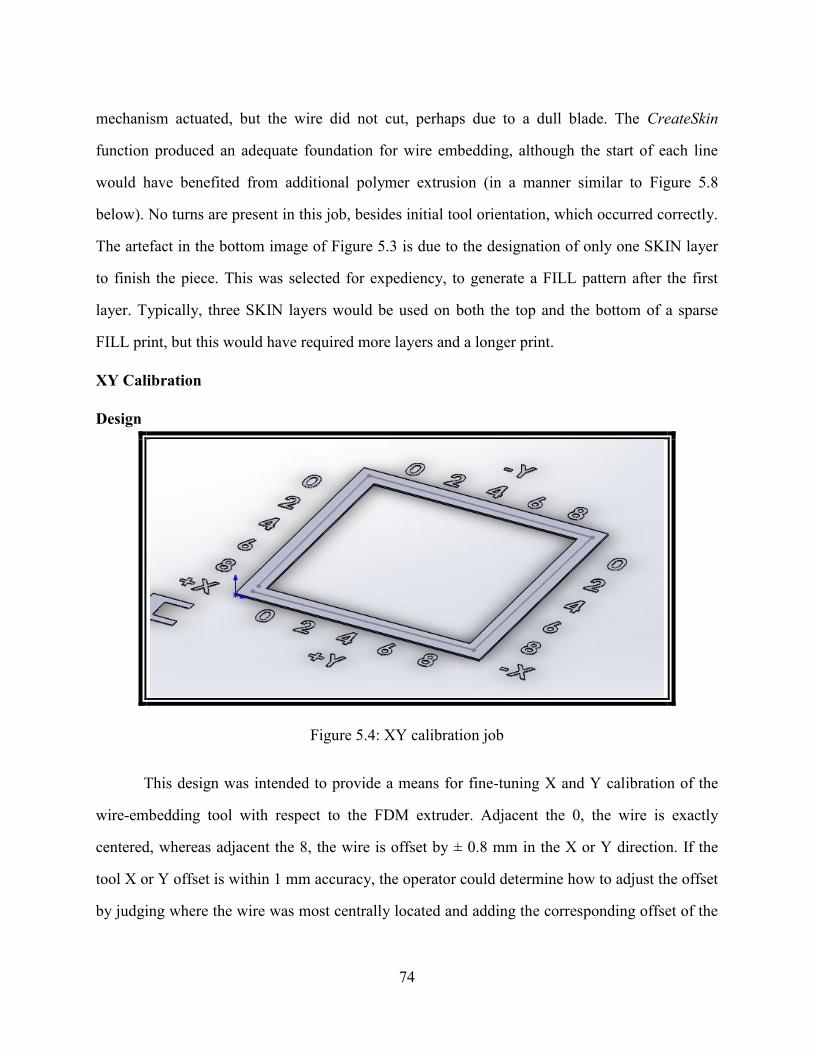
74
mechanism actuated, but the wire did not cut, perhaps due to a dull blade. The CreateSkin
function produced an adequate foundation for wire embedding, although the start of each line
would have benefited from additional polymer extrusion (in a manner similar to Figure 5.8
below). No turns are present in this job, besides initial tool orientation, which occurred correctly.
The artefact in the bottom image of Figure 5.3 is due to the designation of only one SKIN layer
to finish the piece. This was selected for expediency, to generate a FILL pattern after the first
layer. Typically, three SKIN layers would be used on both the top and the bottom of a sparse
FILL print, but this would have required more layers and a longer print.
XY Calibration
Design
Figure 5.4: XY calibration job
This design was intended to provide a means for fine-tuning X and Y calibration of the
wire-embedding tool with respect to the FDM extruder. Adjacent the 0, the wire is exactly
centered, whereas adjacent the 8, the wire is offset by ± 0.8 mm in the X or Y direction. If the
tool X or Y offset is within 1 mm accuracy, the operator could determine how to adjust the offset
by judging where the wire was most centrally located and adding the corresponding offset of the
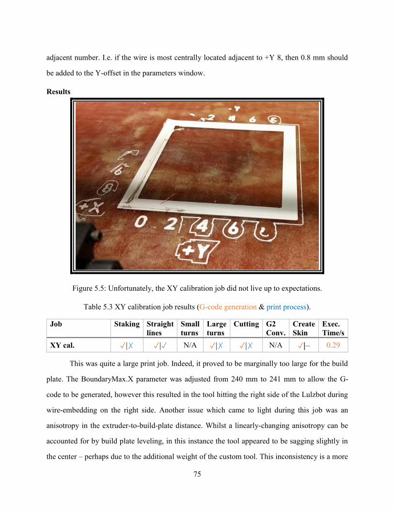
75
adjacent number. I.e. if the wire is most centrally located adjacent to +Y 8, then 0.8 mm should
be added to the Y-offset in the parameters window.
Results
Figure 5.5: Unfortunately, the XY calibration job did not live up to expectations.
Table 5.3 XY calibration job results (G-code generation & print process).
Job Staking Straight
lines
Small
turns
Large
turns
Cutting G2
Conv.
Create
Skin
Exec.
Time/s
XY cal. ✓|✗ ✓|✓ N/A ✓|✗ ✓|✗ N/A ✓|– 0.29
This was quite a large print job. Indeed, it proved to be marginally too large for the build
plate. The BoundaryMax.X parameter was adjusted from 240 mm to 241 mm to allow the G-
code to be generated, however this resulted in the tool hitting the right side of the Lulzbot during
wire-embedding on the right side. Another issue which came to light during this job was an
anisotropy in the extruder-to-build-plate distance. Whilst a linearly-changing anisotropy can be
accounted for by build plate leveling, in this instance the tool appeared to be sagging slightly in
the center – perhaps due to the additional weight of the custom tool. This inconsistency is a more
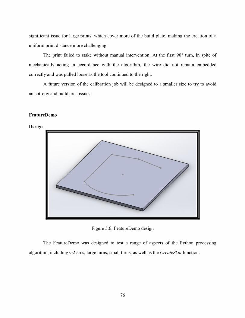
76
significant issue for large prints, which cover more of the build plate, making the creation of a
uniform print distance more challenging.
The print failed to stake without manual intervention. At the first 90° turn, in spite of
mechanically acting in accordance with the algorithm, the wire did not remain embedded
correctly and was pulled loose as the tool continued to the right.
A future version of the calibration job will be designed to a smaller size to try to avoid
anisotropy and build area issues.
FeatureDemo
Design
Figure 5.6: FeatureDemo design
The FeatureDemo was designed to test a range of aspects of the Python processing
algorithm, including G2 arcs, large turns, small turns, as well as the CreateSkin function.
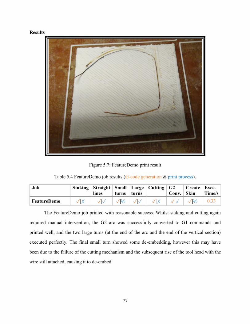
77
Results
Figure 5.7: FeatureDemo print result
Table 5.4 FeatureDemo job results (G-code generation & print process).
Job Staking Straight
lines
Small
turns
Large
turns
Cutting G2
Conv.
Create
Skin
Exec.
Time/s
FeatureDemo ✓|✗ ✓|✓ ✓|½ ✓|✓ ✓|✗ ✓|✓ ✓|½ 0.33
The FeatureDemo job printed with reasonable success. Whilst staking and cutting again
required manual intervention, the G2 arc was successfully converted to G1 commands and
printed well, and the two large turns (at the end of the arc and the end of the vertical section)
executed perfectly. The final small turn showed some de-embedding, however this may have
been due to the failure of the cutting mechanism and the subsequent rise of the tool head with the
wire still attached, causing it to de-embed.
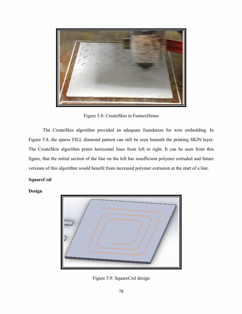
78
Figure 5.8: CreateSkin in FeatureDemo
The CreateSkin algorithm provided an adequate foundation for wire embedding. In
Figure 5.8, the sparse FILL diamond pattern can still be seen beneath the printing SKIN layer.
The CreateSkin algorithm prints horizontal lines from left to right. It can be seen from this
figure, that the initial section of the line on the left has insufficient polymer extruded and future
versions of this algorithm would benefit from increased polymer extrusion at the start of a line.
SquareCoil
Design
Figure 5.9: SquareCoil design
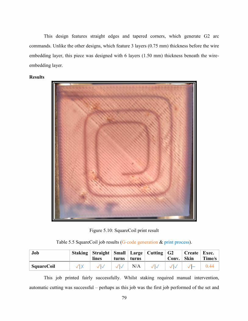
79
This design features straight edges and tapered corners, which generate G2 arc
commands. Unlike the other designs, which feature 3 layers (0.75 mm) thickness before the wire
embedding layer, this piece was designed with 6 layers (1.50 mm) thickness beneath the wire-
embedding layer.
Results
Figure 5.10: SquareCoil print result
Table 5.5 SquareCoil job results (G-code generation & print process).
Job Staking Straight
lines
Small
turns
Large
turns
Cutting G2
Conv.
Create
Skin
Exec.
Time/s
SquareCoil ✓|✗ ✓|✓ ✓|✓ N/A ✓|✓ ✓|✓ ✓|– 0.44
This job printed fairly successfully. Whilst staking required manual intervention,
automatic cutting was successful – perhaps as this job was the first job performed of the set and
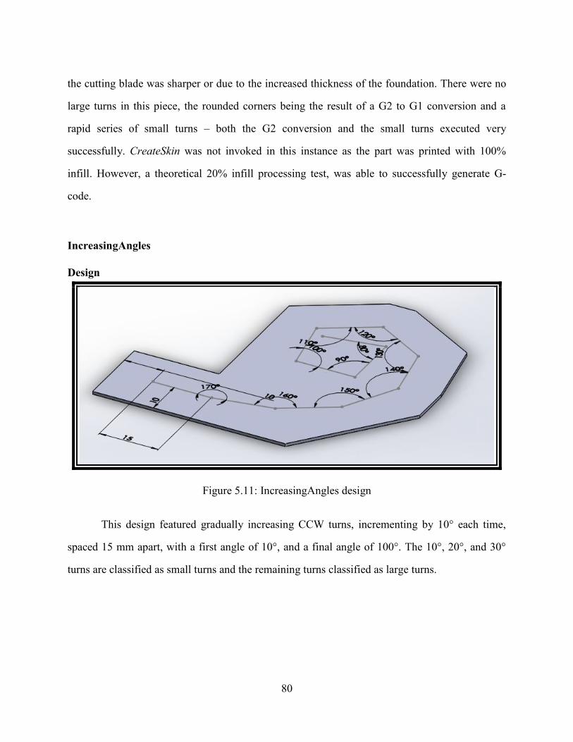
80
the cutting blade was sharper or due to the increased thickness of the foundation. There were no
large turns in this piece, the rounded corners being the result of a G2 to G1 conversion and a
rapid series of small turns – both the G2 conversion and the small turns executed very
successfully. CreateSkin was not invoked in this instance as the part was printed with 100%
infill. However, a theoretical 20% infill processing test, was able to successfully generate G-
code.
IncreasingAngles
Design
Figure 5.11: IncreasingAngles design
This design featured gradually increasing CCW turns, incrementing by 10° each time,
spaced 15 mm apart, with a first angle of 10°, and a final angle of 100°. The 10°, 20°, and 30°
turns are classified as small turns and the remaining turns classified as large turns.
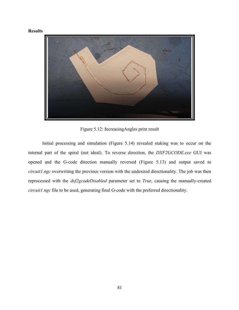
81
Results
Figure 5.12: IncreasingAngles print result
Initial processing and simulation (Figure 5.14) revealed staking was to occur on the
internal part of the spiral (not ideal). To reverse direction, the DXF2GCODE.exe GUI was
opened and the G-code direction manually reversed (Figure 5.13) and output saved to
circuit1.ngc overwriting the previous version with the undesired directionality. The job was then
reprocessed with the dxf2gcodeDisabled parameter set to True, causing the manually-created
circuit1.ngc file to be used, generating final G-code with the preferred directionality.
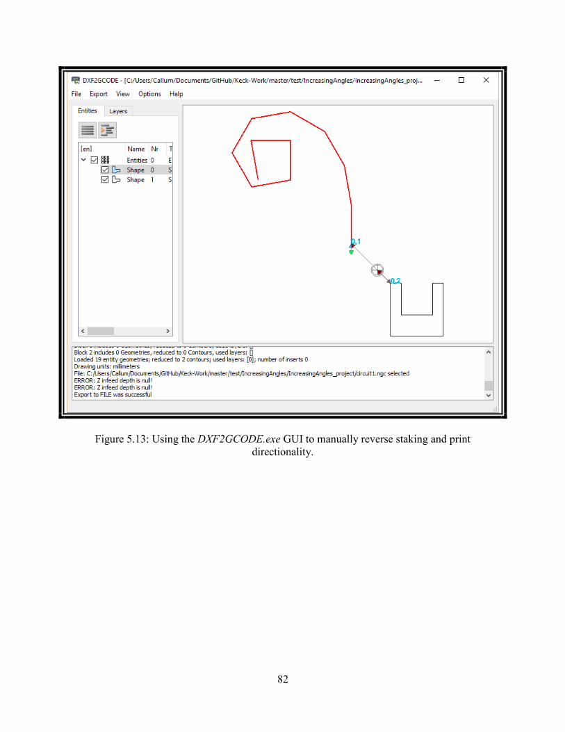
82
Figure 5.13: Using the DXF2GCODE.exe GUI to manually reverse staking and print
directionality.
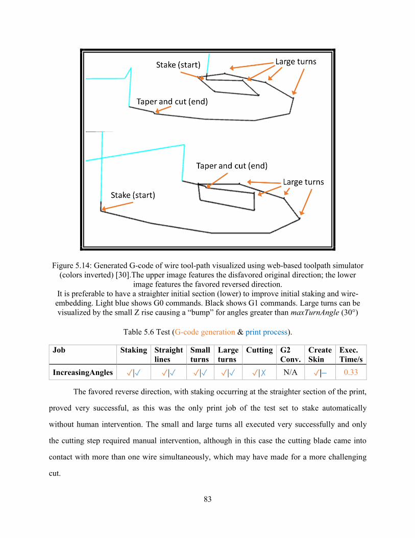
83
Figure 5.14: Generated G-code of wire tool-path visualized using web-based toolpath simulator
(colors inverted) [30].The upper image features the disfavored original direction; the lower
image features the favored reversed direction.
It is preferable to have a straighter initial section (lower) to improve initial staking and wire-
embedding. Light blue shows G0 commands. Black shows G1 commands. Large turns can be
visualized by the small Z rise causing a “bump” for angles greater than maxTurnAngle (30°)
Table 5.6 Test (G-code generation & print process).
Job Staking Straight
lines
Small
turns
Large
turns
Cutting G2
Conv.
Create
Skin
Exec.
Time/s
IncreasingAngles ✓|✓ ✓|✓ ✓|✓ ✓|✓ ✓|✗ N/A ✓|– 0.33
The favored reverse direction, with staking occurring at the straighter section of the print,
proved very successful, as this was the only print job of the test set to stake automatically
without human intervention. The small and large turns all executed very successfully and only
the cutting step required manual intervention, although in this case the cutting blade came into
contact with more than one wire simultaneously, which may have made for a more challenging
cut.
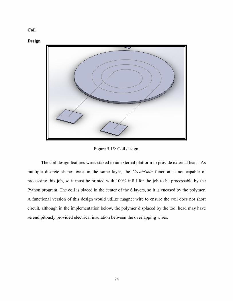
84
Coil
Design
Figure 5.15: Coil design.
The coil design features wires staked to an external platform to provide external leads. As
multiple discrete shapes exist in the same layer, the CreateSkin function is not capable of
processing this job, so it must be printed with 100% infill for the job to be processable by the
Python program. The coil is placed in the center of the 6 layers, so it is encased by the polymer.
A functional version of this design would utilize magnet wire to ensure the coil does not short
circuit, although in the implementation below, the polymer displaced by the tool head may have
serendipitously provided electrical insulation between the overlapping wires.
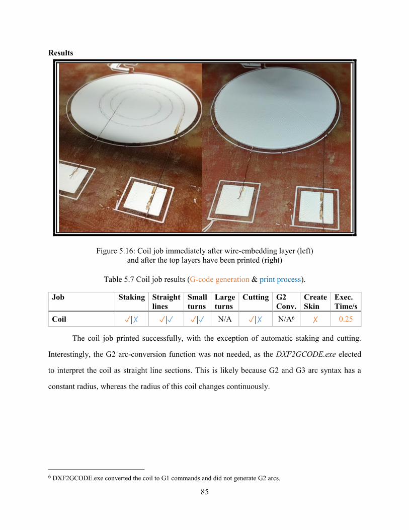
85
Results
Figure 5.16: Coil job immediately after wire-embedding layer (left)
and after the top layers have been printed (right)
Table 5.7 Coil job results (G-code generation & print process).
Job Staking Straight
lines
Small
turns
Large
turns
Cutting G2
Conv.
Create
Skin
Exec.
Time/s
Coil ✓|✗ ✓|✓ ✓|✓ N/A ✓|✗ N/A6 ✗ 0.25
The coil job printed successfully, with the exception of automatic staking and cutting.
Interestingly, the G2 arc-conversion function was not needed, as the DXF2GCODE.exe elected
to interpret the coil as straight line sections. This is likely because G2 and G3 arc syntax has a
constant radius, whereas the radius of this coil changes continuously.
6 DXF2GCODE.exe converted the coil to G1 commands and did not generate G2 arcs.
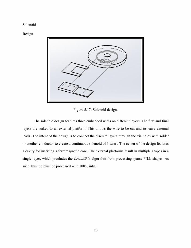
86
Solenoid
Design
Figure 5.17: Solenoid design.
The solenoid design features three embedded wires on different layers. The first and final
layers are staked to an external platform. This allows the wire to be cut and to leave external
leads. The intent of the design is to connect the discrete layers through the via holes with solder
or another conductor to create a continuous solenoid of 3 turns. The center of the design features
a cavity for inserting a ferromagnetic core. The external platforms result in multiple shapes in a
single layer, which precludes the CreateSkin algorithm from processing sparse FILL shapes. As
such, this job must be processed with 100% infill.
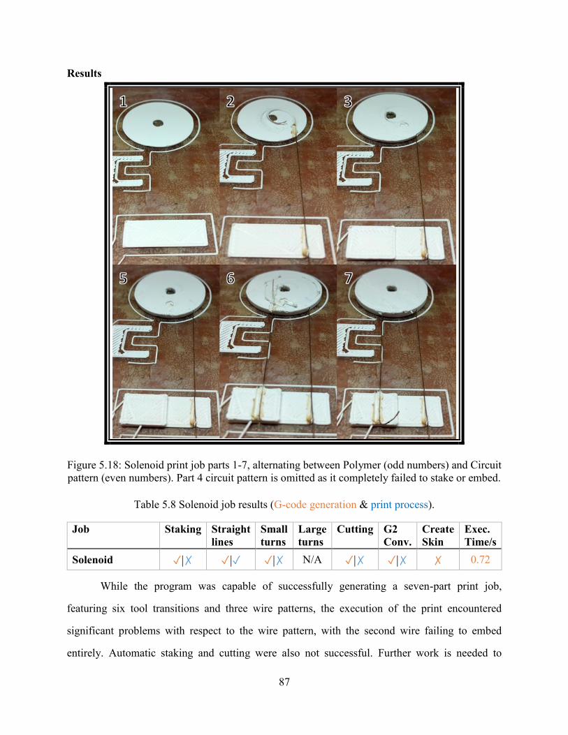
87
Results
Figure 5.18: Solenoid print job parts 1-7, alternating between Polymer (odd numbers) and Circuit
pattern (even numbers). Part 4 circuit pattern is omitted as it completely failed to stake or embed.
Table 5.8 Solenoid job results (G-code generation & print process).
Job Staking Straight
lines
Small
turns
Large
turns
Cutting G2
Conv.
Create
Skin
Exec.
Time/s
Solenoid ✓|✗ ✓|✓ ✓|✗ N/A ✓|✗ ✓|✗ ✗ 0.72
While the program was capable of successfully generating a seven-part print job,
featuring six tool transitions and three wire patterns, the execution of the print encountered
significant problems with respect to the wire pattern, with the second wire failing to embed
entirely. Automatic staking and cutting were also not successful. Further work is needed to

88
determine whether the difficulties encountered are due to the small radius of the circle,
unoptimized process parameters, or limitations of the tool design. One can take heart that the
algorithm was able to successfully generate G-code and tool transitions in the correct sequential
order, with correct wire-embedding tool rotations, without appearing to have any deleterious
effects on the FDM printing process, and that these issues may be solvable through parameter
optimization.
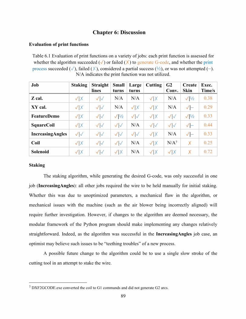
89
Chapter 6: Discussion
Evaluation of print functions
Table 6.1 Evaluation of print functions on a variety of jobs: each print function is assessed for
whether the algorithm succeeded (✓) or failed (✗) to generate G-code, and whether the print
process succeeded (✓), failed (✗), considered a partial success (½), or was not attempted (–).
N/A indicates the print function was not utilized.
Job Staking Straight
lines
Small
turns
Large
turns
Cutting G2
Conv.
Create
Skin
Exec.
Time/s
Z cal. ✓|✗ ✓|✓ N/A N/A ✓|✗ N/A ✓|½ 0.38
XY cal. ✓|✗ ✓|✓ N/A ✓|✗ ✓|✗ N/A ✓|– 0.29
FeatureDemo ✓|✗ ✓|✓ ✓|½ ✓|✓ ✓|✗ ✓|✓ ✓|½ 0.33
SquareCoil ✓|✗ ✓|✓ ✓|✓ N/A ✓|✓ ✓|✓ ✓|– 0.44
IncreasingAngles ✓|✓ ✓|✓ ✓|✓ ✓|✓ ✓|✗ N/A ✓|– 0.33
Coil ✓|✗ ✓|✓ ✓|✓ N/A ✓|✗ N/A7 ✗ 0.25
Solenoid ✓|✗ ✓|✓ ✓|✗ N/A ✓|✗ ✓|✗ ✗ 0.72
Staking
The staking algorithm, while generating the desired G-code, was only successful in one
job (IncreasingAngles): all other jobs required the wire to be held manually for initial staking.
Whether this was due to unoptimized parameters, a mechanical flaw in the algorithm, or
mechanical issues with the machine (such as the air blower being incorrectly aligned) will
require further investigation. However, if changes to the algorithm are deemed necessary, the
modular framework of the Python program should make implementing any changes relatively
straightforward. Indeed, as the algorithm was successful in the IncreasingAngles job case, an
optimist may believe such issues to be “teething troubles” of a new process.
A possible future change to the algorithm could be to use a single slow stroke of the
cutting tool in an attempt to stake the wire.
7 DXF2GCODE.exe converted the coil to G1 commands and did not generate G2 arcs.
90
Straight lines
All jobs were successful in generating G-code and printing embedding straight lines of
wire, so long as the initial staking was implemented (automatically or with manual intervention).
Small turns
In all cases a maxTurnAngle = 30° was used, so small turns are defined as those that
involved a tool rotation of less than or equal to 30°. G-code was generated as intended for all
jobs. Actual print quality showed some variation, with discrete small turns at a vertex generally
implemented more successfully than continuous small turns as part of an arc, although both
instances had successes and failures. As well as parameter optimization, future plans for the tool
include the implementation of an additional small motor to actively feed the wire, instead of
relying on the wire to be passively fed by staking and translational movement of the tool head.
Such an enhancement should reduce the instance of wires “cutting corners” and could be
particularly useful for tight radius circles, such as the solenoid job.
Large turns
Within the test set, large turns had a two-out-of-three success rate for printing. The one
failure occurred on the XY calibration job, which encountered a number of problems related to
its large size and extruder-to-build-plate distance anisotropy. In a broad sense the large-turns
algorithm and its implementation appear to have been successful.
Cutting
Whilst the cutting commands operated as expected, the mechanism of cutting tool did
not, with the exception of the SquareCoil job, which was able to implement a successful cut. It
may be that these print jobs are too thin and the surface polymer too close to its glass transition
temperature to provide a suitably solid surface to cut against. Indeed, with a build plate
temperature of 110 °C and a typical glass transition temperature of ABS in the range of 105 °C,
this may well have been the case. In addition, the one successful cutting job, the SquareCoil,
featured double the foundation thickness of the other print jobs, providing extra thermal
91
insulation from the build plate. Future experiments will be attempted with a lower build plate
temperature.
G2 conversion
G2 arc conversion had mixed fortunes: whilst the algorithm resulted in successful prints
on the SquareCoil and FeatureDemo jobs, the Solenoid job completely failed on the circular
portion. To determine whether this failure was due to the G2 conversion function or due to other
parameters and causes will require further experimentation. However, it appears the algorithm is
fundamentally sound and only parameter optimizations may be required.
CreateSkin
This algorithm, while broadly functional, has plenty of room for improvement, such as
extruding polymer in both left-to-right and right-to-left directions, ensuring adequate polymer is
dispensed initially, and expanding the algorithm to be compatible with more complex designs
featuring multiple shapes in a single layer.
Initially implemented as a quick fix to the problem of providing a foundation for wire-
embedding above a sparse filled interior, a better long term solution may be to implement
existing SKIN generating functionalities from the Cura libraries and developing closer
integration between the Cura slicer and the post-processing program.
Proposed Features and Future Work
Whilst great progress has been made during the development of this multi-material
printing algorithm, a number of areas for improvement remain. One such area would be in
developing automated wire-embedding out of the XY plane. It may be possible to achieve this by
switching design tools, as Autodesk Fusion 360 has shown some promise for multi-process
support and also supports a Python API as opposed to the Visual Basic API of Solidworks. There
is also room to optimize execution speed of the code, if required, as the current implementation
involves many iterations of reading all lines and acting on them sequentially. However, this has
92
not presented an issue for the test files processed so far, which typically exhibit processing times
of less than one second.
Working with the mechanical engineers, who are the primary operators and designers of
the Lulzbot, has revealed GUI interface changes, such as reducing the number of parameters on
the main GUI screen, adding support for changing the G2 arc conversion parameters
(maxArcLength, maxDTheta) in the GUI, and the ability to switch start and end points for wire-
embedding patterns. Many of these features are under implementation by the W.M. Keck Center
for 3D Innovation GUI wunderkind, Jake Lasley. An integrated toolpath simulator is being
developed by Mike Licerio.
Efrain Aguilera, whose work is published concurrently, has made progress in developing
support for importing defined print cavities directly into Solidworks from integrated circuit
components defined by modified Cadsoft EAGLE hardware libraries. This lays the groundwork
for automatically incorporating interconnected integrated circuits into FDM designs.
93
References
[1] C. W. Hull, “Apparatus for production of three-dimensional objects by
stereolithography,” US4575330 A, 11-Mar-1986.
[2] K. V. Wong and A. Hernandez, “A review of additive manufacturing,” ISRN Mech. Eng.,
vol. 2012, 2012.
[3] M. S. Mannoor et al., “3D printed bionic ears,” Nano Lett., vol. 13, no. 6, pp. 2634–2639,
2013.
[4] J. Norman, R. D. Madurawe, C. M. Moore, M. A. Khan, and A. Khairuzzaman, “A new
chapter in pharmaceutical manufacturing: 3D-printed drug products,” Adv. Drug Deliv. Rev.,
2016.
[5] R. R. Koreis, “Three Dimensional Printing of Parts,” US20150064299 A1, 05-Mar-2015.
[6] E. Sachs, E. Wylonis, S. Allen, M. Cima, and H. Guo, “Production of injection molding
tooling with conformal cooling channels using the three dimensional printing process,” Polym.
Eng. Sci., vol. 40, no. 5, pp. 1232–1247, 2000.
[7] B. Berman, “3-D printing: The new industrial revolution,” Bus. Horiz., vol. 55, no. 2, pp.
155–162, 2012.
[8] “Art - Shapeways 3D Printing,” Shapeways.com. [Online]. Available: /marketplace/art/.
[Accessed: 19-Oct-2016].
[9] S. S. Crump, “Apparatus and method for creating three-dimensional objects,”
US5121329 A, 09-Jun-1992.
[10] “Extrusion deposition: Fused Deposition Modeling (FDM),” additive3d.com, 18-Aug-
2016. .
[11] L. E. Roscoe and others, “Stereolithography interface specification,” Am.-3D Syst. Inc,
1988.
[12] C. Shemelya et al., “3D printed capacitive sensors,” in SENSORS, 2013 IEEE, 2013, pp.
1–4.
[13] A. Kataria and D. W. Rosen, “Building around inserts: methods for fabricating complex
devices in stereolithography,” Rapid Prototyp. J., vol. 7, no. 5, pp. 253–262, 2001.
[14] J. A. Palmer et al., “Rapid prototyping of high density circuitry,” in Proc. Rapid
Prototyping & Manufacturing 2004 Conference Proceedings, 2004, pp. 10–13.
[15] F. Medina et al., “Integrating multiple rapid manufacturing technologies for developing
advanced customized functional devices,” in Proc. Rapid Prototyping & Manufacturing 2005
Conference Proceedings, 2005, pp. 10–12.
[16] F. Medina et al., “Hybrid manufacturing: integrating direct-write and stereolithography,”
Proc. 2005 Solid Free. Fabr. J. Manuf. Sci. Eng., 2005.
[17] D. Espalin, D. W. Muse, E. MacDonald, and R. B. Wicker, “3D Printing
multifunctionality: structures with electronics,” Int. J. Adv. Manuf. Technol., vol. 72, no. 5–8,
pp. 963–978, 2014.
[18] C. Tröger, A. T. Bens, G. Bermes, R. Klemmer, J. Lenz, and S. Irsen, “Ageing of
acrylate-based resins for stereolithography: thermal and humidity ageing behaviour studies,”
Rapid Prototyp. J., vol. 14, no. 5, pp. 305–317, 2008.
[19] B. Salam, W. L. Lai, L. C. W. Albert, and L. B. Keng, “Low temperature processing of
copper conductive ink for printed electronics applications,” in Electronics Packaging
Technology Conference (EPTC), 2011 IEEE 13th, 2011, pp. 251–255.

94
[20] “Functional Materials,” Voxel8. [Online]. Available: http://www.voxel8.com/materials/.
[Accessed: 17-Oct-2016].
[21] D. A. Marquez, “Development of the thermal wire embedding technology for electronic
and mechanical applications on FDM-printed parts,” THE UNIVERSITY OF TEXAS AT EL
PASO, 2016.
[22] E. MacDonald and R. Wicker, “Multiprocess 3D printing for increasing component
functionality,” Science, vol. 353, no. 6307, p. aaf2093, Sep. 2016.
[23] W. M. Marshall et al., “Using Additive Manufacturing to Print a CubeSat Propulsion
System,” in 51st AIAA/SAE/ASEE Joint Propulsion Conference, 2015, p. 4184.
[24] F. Wasserfall, “Conductive Printing Project.” [Online]. Available:
https://tams.informatik.uni-hamburg.de/research/3d-printing/conductive_printing/. [Accessed:
19-Oct-2016].
[25] F. Wasserfall, “Embedding of SMD populated circuits into FDM printed objects,” in
Proceedings of the 2015 Solid Freeform Fabrication., 2015, pp. 180–189.
[26] “Bridging the ECAD/MCAD gap with Fusion 360 and CadSoft EAGLE,” DESIGN
DIFFERENTLY, 11-Dec-2015. [Online]. Available: http://www.autodesk.com/products/fusion-
360/blog/bridging-the-ecadmcad-gap-with-fusion-360-and-cadsoft-eagle/. [Accessed: 19-Oct-
2016].
[27] E. Aguilera, “Creating Multi-functional G-code for Multi-process Additive
Manufacturing,” Master’s Thesis, The University of Texas at El Paso, 2016.
[28] “dxf2gcode,” SourceForge. [Online]. Available:
https://sourceforge.net/projects/dxf2gcode/. [Accessed: 12-Nov-2016].
[29] “pyclipper 1.0.5 : Python Package Index.” [Online]. Available:
https://pypi.python.org/pypi/pyclipper. [Accessed: 26-Nov-2016].
[30] “g-code simulator.” [Online]. Available: https://nraynaud.github.io/webgcode/.
[Accessed: 20-Nov-2016].
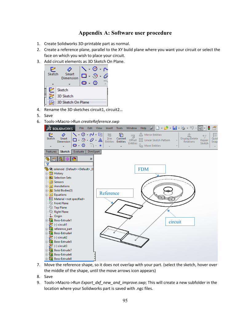
95
Appendix A: Software user procedure
1. Create Solidworks 3D-printable part as normal.
2. Create a reference plane, parallel to the XY build plane where you want your circuit or select the
face on which you wish to place your circuit.
3. Add circuit elements as 3D Sketch On Plane.
4. Rename�the�3D�sketches�circuit1,�circuit2…
5. Save
6. Tools->Macro->Run createReference.swp
7. Move the reference shape, so it does not overlap with your part. (select the sketch, hover over
the middle of the shape, until the move arrows icon appears)
8. Save
9. Tools->Macro->Run Export_dxf_new_and_improve.swp; This will create a new subfolder in the
location where your Solidworks part is saved with .ngc files.
Reference
shape
circuit
wires
FDM
design
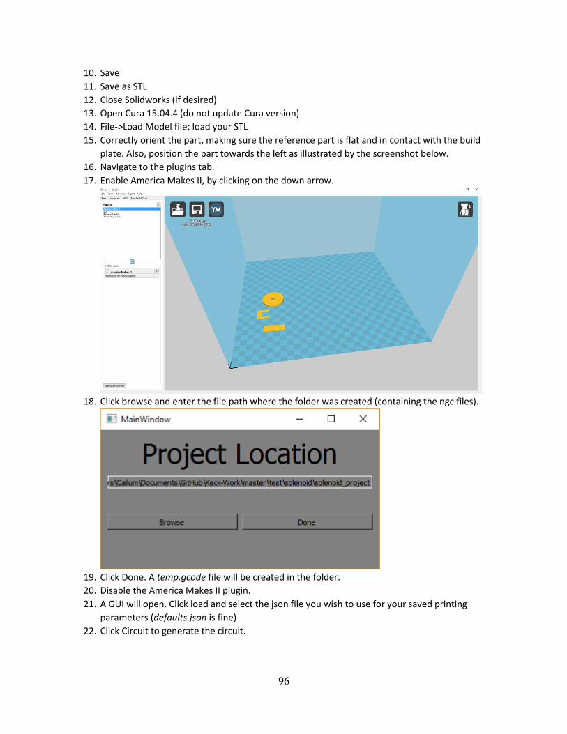
96
10. Save
11. Save as STL
12. Close Solidworks (if desired)
13. Open Cura 15.04.4 (do not update Cura version)
14. File->Load Model file; load your STL
15. Correctly orient the part, making sure the reference part is flat and in contact with the build
plate. Also, position the part towards the left as illustrated by the screenshot below.
16. Navigate to the plugins tab.
17. Enable America Makes II, by clicking on the down arrow.
18. Click browse and enter the file path where the folder was created (containing the ngc files).
19. Click Done. A temp.gcode file will be created in the folder.
20. Disable the America Makes II plugin.
21. A GUI will open. Click load and select the json file you wish to use for your saved printing
parameters (defaults.json is fine)
22. Click Circuit to generate the circuit.
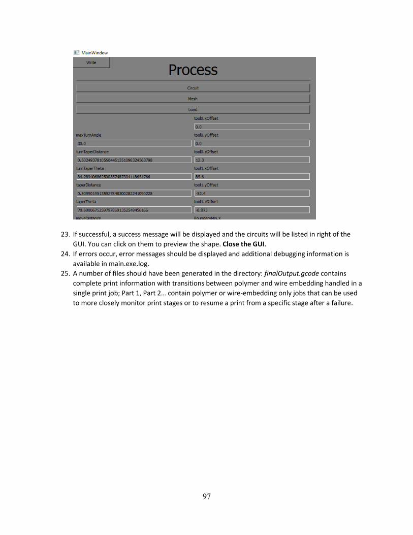
97
23. If successful, a success message will be displayed and the circuits will be listed in right of the
GUI. You can click on them to preview the shape. Close the GUI.
24. If errors occur, error messages should be displayed and additional debugging information is
available in main.exe.log.
25. A number of files should have been generated in the directory: finalOutput.gcode contains
complete print information with transitions between polymer and wire embedding handled in a
single�print�job;�Part�1,�Part�2…�contain�polymer�or�wire-embedding only jobs that can be used
to more closely monitor print stages or to resume a print from a specific stage after a failure.

98
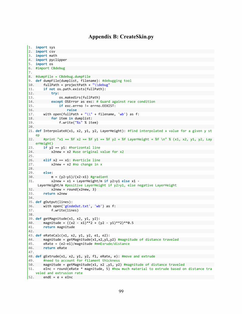
99
Appendix B: CreateSkin.py
1. import sys 2. import csv 3. import math 4. import pyclipper 5. import os 6. #import CBdebug 7. 8. #dumpFile = CBdebug.dumpFile 9. def dumpFile(dumplist, filename): #debugging tool 10. fullPath = projectPath + "\\debug" 11. if not os.path.exists(fullPath): 12. try: 13. os.makedirs(fullPath) 14. except OSError as exc: # Guard against race condition 15. if exc.errno != errno.EEXIST: 16. raise 17. with open(fullPath + "\\" + filename, 'wb') as f: 18. for item in dumplist: 19. f.write("%s" % item) 20. 21. def InterpolateX(x1, x2, y1, y2, LayerHeight): #find interpolated x value for a given y st
ep 22. #print "x1 == %f x2 == %f y1 == %f y2 = %f LayerHeight = %f \n" % (x1, x2, y1, y2, Lay
erHeight) 23. if y2 == y1: #horizontal line 24. x2new = x2 #use original value for x2 25. 26. elif x2 == x1: #verticle line 27. x2new = x2 #no change in x 28. 29. else: 30. m = (y2-y1)/(x2-x1) #gradient 31. x2new = x1 + LayerHeight/m if y2>y1 else x1 -
LayerHeight/m #positive LayerHeight if y2>y1, else negative LayerHeight 32. x2new = round(x2new, 3) 33. return x2new 34. 35. def gOutput(lines): 36. with open('gCodeOut.txt', 'wb') as f: 37. f.write(lines) 38. 39. def getMagnitude(x1, x2, y1, y2): 40. magnitude = ((x2 - x1)**2 + (y2 - y1)**2)**0.5 41. return magnitude 42. 43. def eRateCalc(x1, x2, y1, y2, e1, e2): 44. magnitude = getMagnitude(x1,x2,y1,y2) #magnitude of distance traveled 45. eRate = (e2-e1)/magnitude #mmExrude/distance 46. return eRate 47. 48. def gExtrude(x1, x2, y1, y2, f1, eRate, e): #move and extrude 49. #need to account for filament thickness 50. magnitude = getMagnitude(x1, x2 ,y1, y2) #magnitude of distance traveled 51. eInc = round(eRate * magnitude, 5) #how much material to extrude based on distance tra
veled and extrusion rate 52. endE = e + eInc
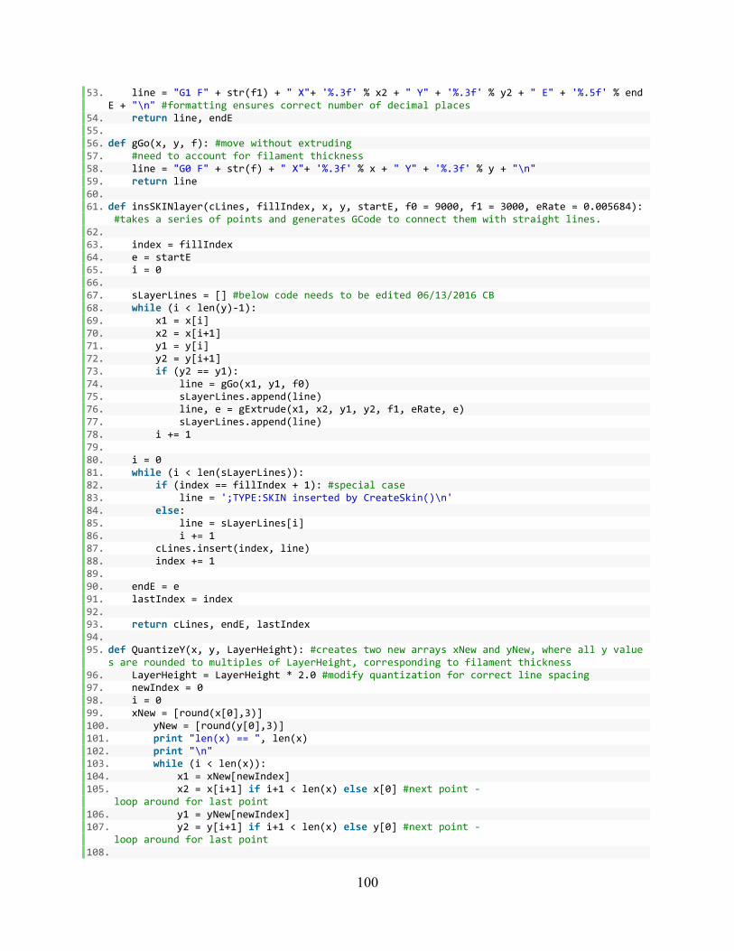
100
53. line = "G1 F" + str(f1) + " X"+ '%.3f' % x2 + " Y" + '%.3f' % y2 + " E" + '%.5f' % endE + "\n" #formatting ensures correct number of decimal places
54. return line, endE 55. 56. def gGo(x, y, f): #move without extruding 57. #need to account for filament thickness 58. line = "G0 F" + str(f) + " X"+ '%.3f' % x + " Y" + '%.3f' % y + "\n" 59. return line 60. 61. def insSKINlayer(cLines, fillIndex, x, y, startE, f0 = 9000, f1 = 3000, eRate = 0.005684):
#takes a series of points and generates GCode to connect them with straight lines. 62. 63. index = fillIndex 64. e = startE 65. i = 0 66. 67. sLayerLines = [] #below code needs to be edited 06/13/2016 CB 68. while (i < len(y)-1): 69. x1 = x[i] 70. x2 = x[i+1] 71. y1 = y[i] 72. y2 = y[i+1] 73. if (y2 == y1): 74. line = gGo(x1, y1, f0) 75. sLayerLines.append(line) 76. line, e = gExtrude(x1, x2, y1, y2, f1, eRate, e) 77. sLayerLines.append(line) 78. i += 1 79. 80. i = 0 81. while (i < len(sLayerLines)): 82. if (index == fillIndex + 1): #special case 83. line = ';TYPE:SKIN inserted by CreateSkin()\n' 84. else: 85. line = sLayerLines[i] 86. i += 1 87. cLines.insert(index, line) 88. index += 1 89. 90. endE = e 91. lastIndex = index 92. 93. return cLines, endE, lastIndex 94. 95. def QuantizeY(x, y, LayerHeight): #creates two new arrays xNew and yNew, where all y value
s are rounded to multiples of LayerHeight, corresponding to filament thickness 96. LayerHeight = LayerHeight * 2.0 #modify quantization for correct line spacing 97. newIndex = 0 98. i = 0 99. xNew = [round(x[0],3)] 100. yNew = [round(y[0],3)] 101. print "len(x) == ", len(x) 102. print "\n" 103. while (i < len(x)): 104. x1 = xNew[newIndex] 105. x2 = x[i+1] if i+1 < len(x) else x[0] #next point -
loop around for last point 106. y1 = yNew[newIndex] 107. y2 = y[i+1] if i+1 < len(x) else y[0] #next point -
loop around for last point 108.
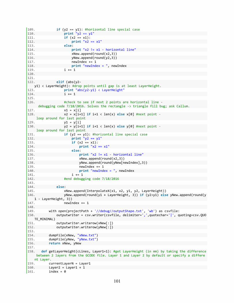
101
109. if (y2 == y1): #horizontal line special case 110. print "y2 == y1" 111. if (x2 == x1): 112. print "x2 == x1" 113. else: 114. print "x2 != x1 - horizontal line" 115. xNew.append(round(x2,3)) 116. yNew.append(round(y2,3)) 117. newIndex += 1 118. print "newIndex = ", newIndex 119. i += 1 120. 121. 122. elif (abs(y2-
y1) < LayerHeight): #drop points until gap is at least LayerHeight. 123. print "abs(y2-y1) < LayerHeight" 124. i += 1 125. 126. #check to see if next 2 points are horizontal line -
debugging code 7/18/2016. Solves the rectangle -> triangle fill bug; ask Callum. 127. x1 = x[i] 128. x2 = x[i+1] if i+1 < len(x) else x[0] #next point -
loop around for last point 129. y1 = y[i] 130. y2 = y[i+1] if i+1 < len(x) else y[0] #next point -
loop around for last point 131. if (y2 == y1): #horizontal line special case 132. print "y2 == y1" 133. if (x2 == x1): 134. print "x2 == x1" 135. else: 136. print "x2 != x1 - horizontal line" 137. xNew.append(round(x2,3)) 138. yNew.append(round(yNew[newIndex],3)) 139. newIndex += 1 140. print "newIndex = ", newIndex 141. i += 1 142. #end debugging code 7/18/2016 143. 144. else: 145. xNew.append(InterpolateX(x1, x2, y1, y2, LayerHeight)) 146. yNew.append(round(y1 + LayerHeight, 3)) if (y2>y1) else yNew.append(round(y
1 - LayerHeight, 3)) 147. newIndex += 1 148. 149. with open(projectPath + '//debug//outputShape.txt', 'wb') as csvfile: 150. outputwriter = csv.writer(csvfile, delimiter=',',quotechar='|', quoting=csv.QUO
TE_MINIMAL) 151. outputwriter.writerow(xNew[:]) 152. outputwriter.writerow(yNew[:]) 153. 154. dumpFile(xNew, "xNew.txt") 155. dumpFile(yNew, "yNew.txt") 156. return xNew, yNew 157. 158. def getLayerHeight(cLines, Layer1=1): #get LayerHeight (in mm) by taking the difference
between 2 layers from the GCODE file. Layer 1 and Layer 2 by default or specify a different Layer.
159. currentLayerN = Layer1 160. Layer2 = Layer1 + 1 161. index = 0
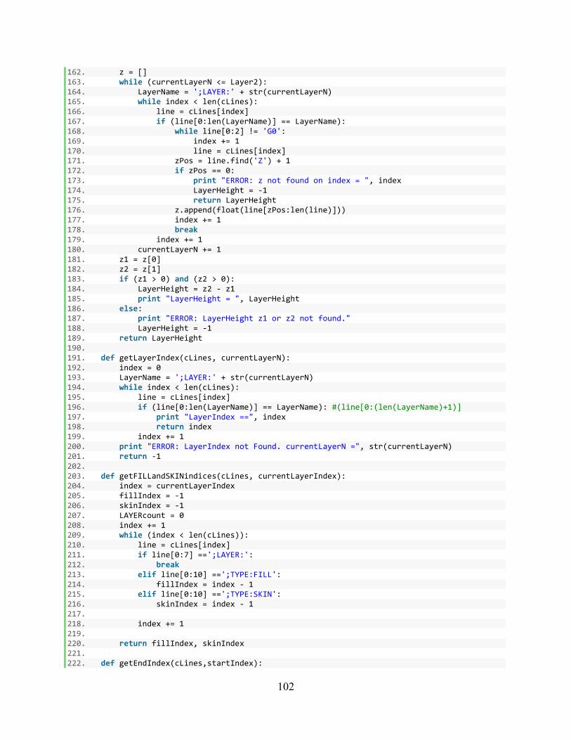
102
162. z = [] 163. while (currentLayerN <= Layer2): 164. LayerName = ';LAYER:' + str(currentLayerN) 165. while index < len(cLines): 166. line = cLines[index] 167. if (line[0:len(LayerName)] == LayerName): 168. while line[0:2] != 'G0': 169. index += 1 170. line = cLines[index] 171. zPos = line.find('Z') + 1 172. if zPos == 0: 173. print "ERROR: z not found on index = ", index 174. LayerHeight = -1 175. return LayerHeight 176. z.append(float(line[zPos:len(line)])) 177. index += 1 178. break 179. index += 1 180. currentLayerN += 1 181. z1 = z[0] 182. z2 = z[1] 183. if (z1 > 0) and (z2 > 0): 184. LayerHeight = z2 - z1 185. print "LayerHeight = ", LayerHeight 186. else: 187. print "ERROR: LayerHeight z1 or z2 not found." 188. LayerHeight = -1 189. return LayerHeight 190. 191. def getLayerIndex(cLines, currentLayerN): 192. index = 0 193. LayerName = ';LAYER:' + str(currentLayerN) 194. while index < len(cLines): 195. line = cLines[index] 196. if (line[0:len(LayerName)] == LayerName): #(line[0:(len(LayerName)+1)] 197. print "LayerIndex ==", index 198. return index 199. index += 1 200. print "ERROR: LayerIndex not Found. currentLayerN =", str(currentLayerN) 201. return -1 202. 203. def getFILLandSKINindices(cLines, currentLayerIndex): 204. index = currentLayerIndex 205. fillIndex = -1 206. skinIndex = -1 207. LAYERcount = 0 208. index += 1 209. while (index < len(cLines)): 210. line = cLines[index] 211. if line[0:7] ==';LAYER:': 212. break 213. elif line[0:10] ==';TYPE:FILL': 214. fillIndex = index - 1 215. elif line[0:10] ==';TYPE:SKIN': 216. skinIndex = index - 1 217. 218. index += 1 219. 220. return fillIndex, skinIndex 221. 222. def getEndIndex(cLines,startIndex):
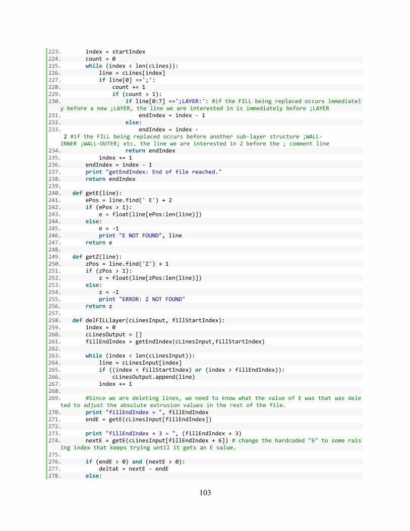
103
223. index = startIndex 224. count = 0 225. while (index < len(cLines)): 226. line = cLines[index] 227. if line[0] ==';': 228. count += 1 229. if (count > 1): 230. if line[0:7] ==';LAYER:': #if the FILL being replaced occurs immediatel
y before a new ;LAYER, the line we are interested in is immediately before ;LAYER 231. endIndex = index - 1 232. else: 233. endIndex = index -
2 #if the FILL being replaced occurs before another sub-layer structure ;WALL-INNER ;WALL-OUTER; etc. the line we are interested in 2 before the ; comment line
234. return endIndex 235. index += 1 236. endIndex = index - 1 237. print "getEndIndex: End of file reached." 238. return endIndex 239. 240. def getE(line): 241. ePos = line.find(' E') + 2 242. if (ePos > 1): 243. e = float(line[ePos:len(line)]) 244. else: 245. e = -1 246. print "E NOT FOUND", line 247. return e 248. 249. def getZ(line): 250. zPos = line.find('Z') + 1 251. if (zPos > 1): 252. z = float(line[zPos:len(line)]) 253. else: 254. z = -1 255. print "ERROR: Z NOT FOUND" 256. return z 257. 258. def delFILLlayer(cLinesInput, fillStartIndex): 259. index = 0 260. cLinesOutput = [] 261. fillEndIndex = getEndIndex(cLinesInput,fillStartIndex) 262. 263. while (index < len(cLinesInput)): 264. line = cLinesInput[index] 265. if ((index < fillStartIndex) or (index > fillEndIndex)): 266. cLinesOutput.append(line) 267. index += 1 268. 269. #Since we are deleting lines, we need to know what the value of E was that was dele
ted to adjust the absolute extrusion values in the rest of the file. 270. print "fillEndIndex = ", fillEndIndex 271. endE = getE(cLinesInput[fillEndIndex]) 272. 273. print "fillEndIndex + 3 = ", (fillEndIndex + 3) 274. nextE = getE(cLinesInput[fillEndIndex + 6]) # change the hardcoded "6" to some rais
ing index that keeps trying until it gets an E value. 275. 276. if (endE > 0) and (nextE > 0): 277. deltaE = nextE - endE 278. else:
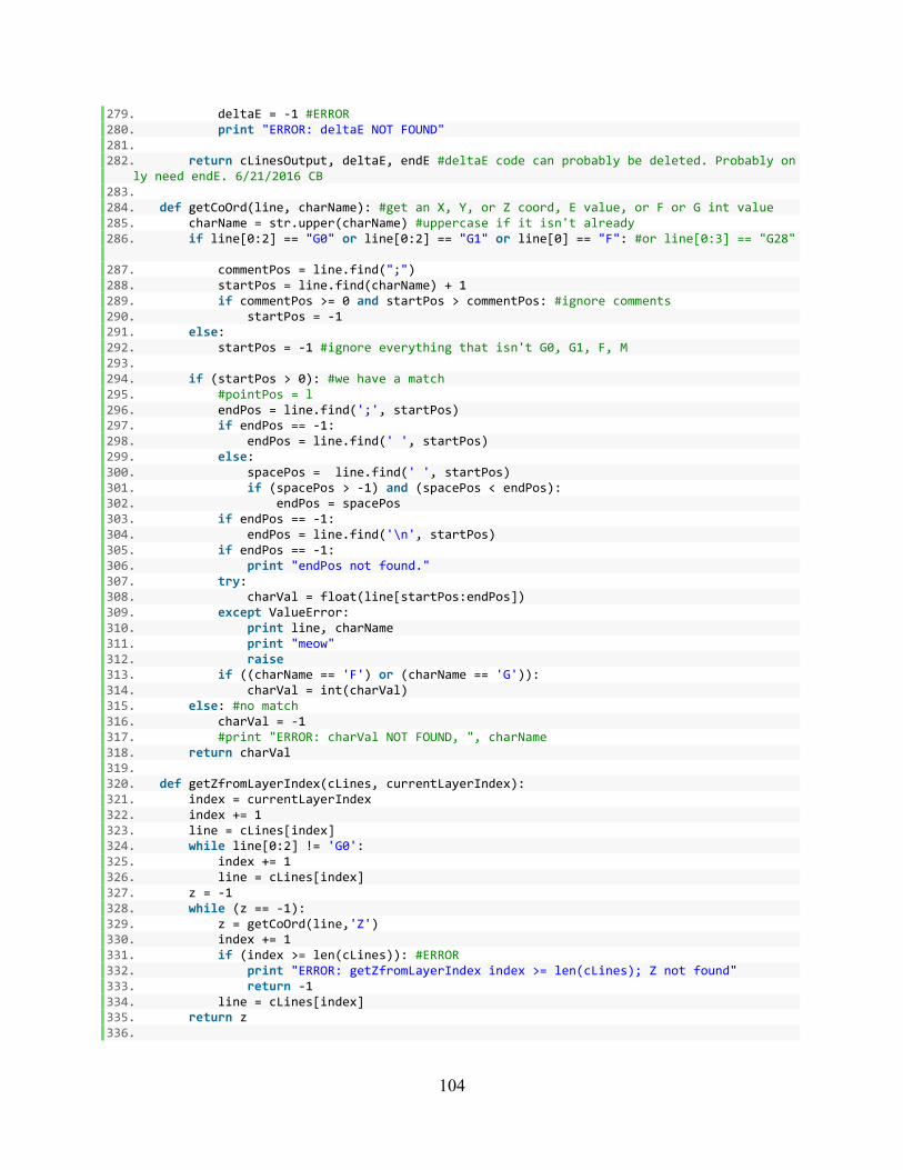
104
279. deltaE = -1 #ERROR 280. print "ERROR: deltaE NOT FOUND" 281. 282. return cLinesOutput, deltaE, endE #deltaE code can probably be deleted. Probably on
ly need endE. 6/21/2016 CB 283. 284. def getCoOrd(line, charName): #get an X, Y, or Z coord, E value, or F or G int value 285. charName = str.upper(charName) #uppercase if it isn't already 286. if line[0:2] == "G0" or line[0:2] == "G1" or line[0] == "F": #or line[0:3] == "G28"
287. commentPos = line.find(";") 288. startPos = line.find(charName) + 1 289. if commentPos >= 0 and startPos > commentPos: #ignore comments 290. startPos = -1 291. else: 292. startPos = -1 #ignore everything that isn't G0, G1, F, M 293. 294. if (startPos > 0): #we have a match 295. #pointPos = l 296. endPos = line.find(';', startPos) 297. if endPos == -1: 298. endPos = line.find(' ', startPos) 299. else: 300. spacePos = line.find(' ', startPos) 301. if (spacePos > -1) and (spacePos < endPos): 302. endPos = spacePos 303. if endPos == -1: 304. endPos = line.find('\n', startPos) 305. if endPos == -1: 306. print "endPos not found." 307. try: 308. charVal = float(line[startPos:endPos]) 309. except ValueError: 310. print line, charName 311. print "meow" 312. raise 313. if ((charName == 'F') or (charName == 'G')): 314. charVal = int(charVal) 315. else: #no match 316. charVal = -1 317. #print "ERROR: charVal NOT FOUND, ", charName 318. return charVal 319. 320. def getZfromLayerIndex(cLines, currentLayerIndex): 321. index = currentLayerIndex 322. index += 1 323. line = cLines[index] 324. while line[0:2] != 'G0': 325. index += 1 326. line = cLines[index] 327. z = -1 328. while (z == -1): 329. z = getCoOrd(line,'Z') 330. index += 1 331. if (index >= len(cLines)): #ERROR 332. print "ERROR: getZfromLayerIndex index >= len(cLines); Z not found" 333. return -1 334. line = cLines[index] 335. return z 336.
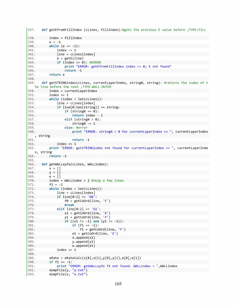
105
337. def getEfromFillIndex (cLines, fillIndex):#gets the previous E value before ;TYPE:FILL
338. index = fillIndex 339. e = -1 340. while (e == -1): 341. index -= 1 342. line = cLines[index] 343. e = getE(line) 344. if (index <= 0): #ERROR 345. print "ERROR: getEfromFillIndex index <= 0; E not found" 346. return -1 347. return e 348. 349. def getSTRINGindex(cLines, currentLayerIndex, stringN, string): #returns the index of t
he line before the text ;TYPE:WALL-OUTER 350. index = currentLayerIndex 351. index += 1 352. while (index < len(cLines)): 353. line = cLines[index] 354. if line[0:len(string)] == string: 355. if (stringN == 0): 356. return index - 1 357. elif (stringN > 0): 358. stringN -= 1 359. else: #error 360. print "ERROR: stringN < 0 for currentLayerIndex == ", currentLayerIndex
, string 361. return -1 362. index += 1 363. print "ERROR: getSTRINGindex not found for currentLayerIndex == ", currentLayerInde
x, string 364. return -1 365. 366. def getWALLxyfe(cLines, WALLindex): 367. x = [] 368. y = [] 369. e = [] 370. index = WALLindex + 2 #skip a few lines 371. f1 = -1 372. while (index < len(cLines)): 373. line = cLines[index] 374. if line[0:2] == 'G0': 375. f0 = getCoOrd(line, 'F') 376. break 377. elif line[0:2] == 'G1': 378. x1 = getCoOrd(line, 'X') 379. y1 = getCoOrd(line, 'Y') 380. if ((x1 != -1) and (y1 != -1)): 381. if (f1 == -1): 382. f1 = getCoOrd(line, 'F') 383. e1 = getCoOrd(line, 'E') 384. x.append(x1) 385. y.append(y1) 386. e.append(e1) 387. index += 1 388. 389. eRate = eRateCalc(x[0],x[1],y[0],y[1],e[0],e[1]) 390. if f1 == -1: 391. print "ERROR: getWALLxyfe f1 not found. WALLindex = ",WALLindex 392. dumpFile(y, "y.txt") 393. dumpFile(x, "x.txt")
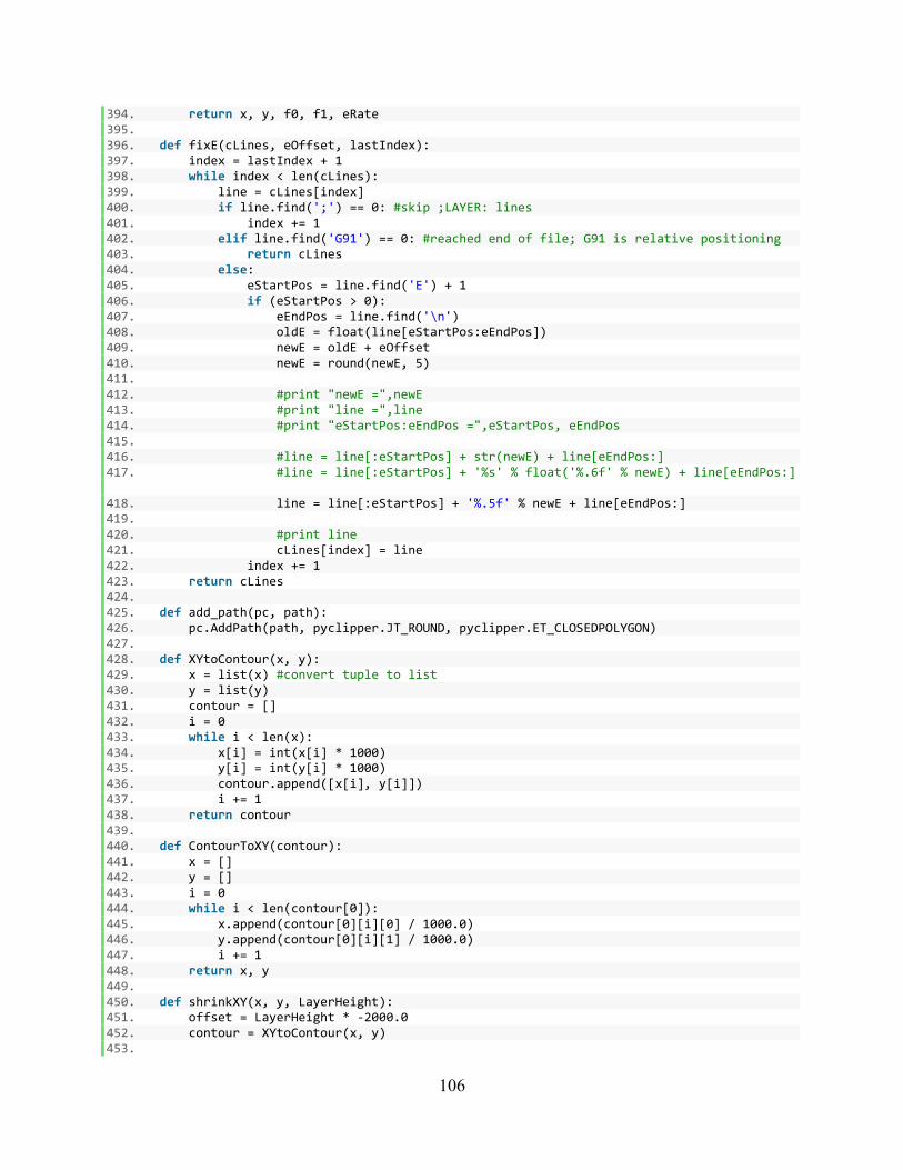
106
394. return x, y, f0, f1, eRate 395. 396. def fixE(cLines, eOffset, lastIndex): 397. index = lastIndex + 1 398. while index < len(cLines): 399. line = cLines[index] 400. if line.find(';') == 0: #skip ;LAYER: lines 401. index += 1 402. elif line.find('G91') == 0: #reached end of file; G91 is relative positioning 403. return cLines 404. else: 405. eStartPos = line.find('E') + 1 406. if (eStartPos > 0): 407. eEndPos = line.find('\n') 408. oldE = float(line[eStartPos:eEndPos]) 409. newE = oldE + eOffset 410. newE = round(newE, 5) 411. 412. #print "newE =",newE 413. #print "line =",line 414. #print "eStartPos:eEndPos =",eStartPos, eEndPos 415. 416. #line = line[:eStartPos] + str(newE) + line[eEndPos:] 417. #line = line[:eStartPos] + '%s' % float('%.6f' % newE) + line[eEndPos:]
418. line = line[:eStartPos] + '%.5f' % newE + line[eEndPos:] 419. 420. #print line 421. cLines[index] = line 422. index += 1 423. return cLines 424. 425. def add_path(pc, path): 426. pc.AddPath(path, pyclipper.JT_ROUND, pyclipper.ET_CLOSEDPOLYGON) 427. 428. def XYtoContour(x, y): 429. x = list(x) #convert tuple to list 430. y = list(y) 431. contour = [] 432. i = 0 433. while i < len(x): 434. x[i] = int(x[i] * 1000) 435. y[i] = int(y[i] * 1000) 436. contour.append([x[i], y[i]]) 437. i += 1 438. return contour 439. 440. def ContourToXY(contour): 441. x = [] 442. y = [] 443. i = 0 444. while i < len(contour[0]): 445. x.append(contour[0][i][0] / 1000.0) 446. y.append(contour[0][i][1] / 1000.0) 447. i += 1 448. return x, y 449. 450. def shrinkXY(x, y, LayerHeight): 451. offset = LayerHeight * -2000.0 452. contour = XYtoContour(x, y) 453.
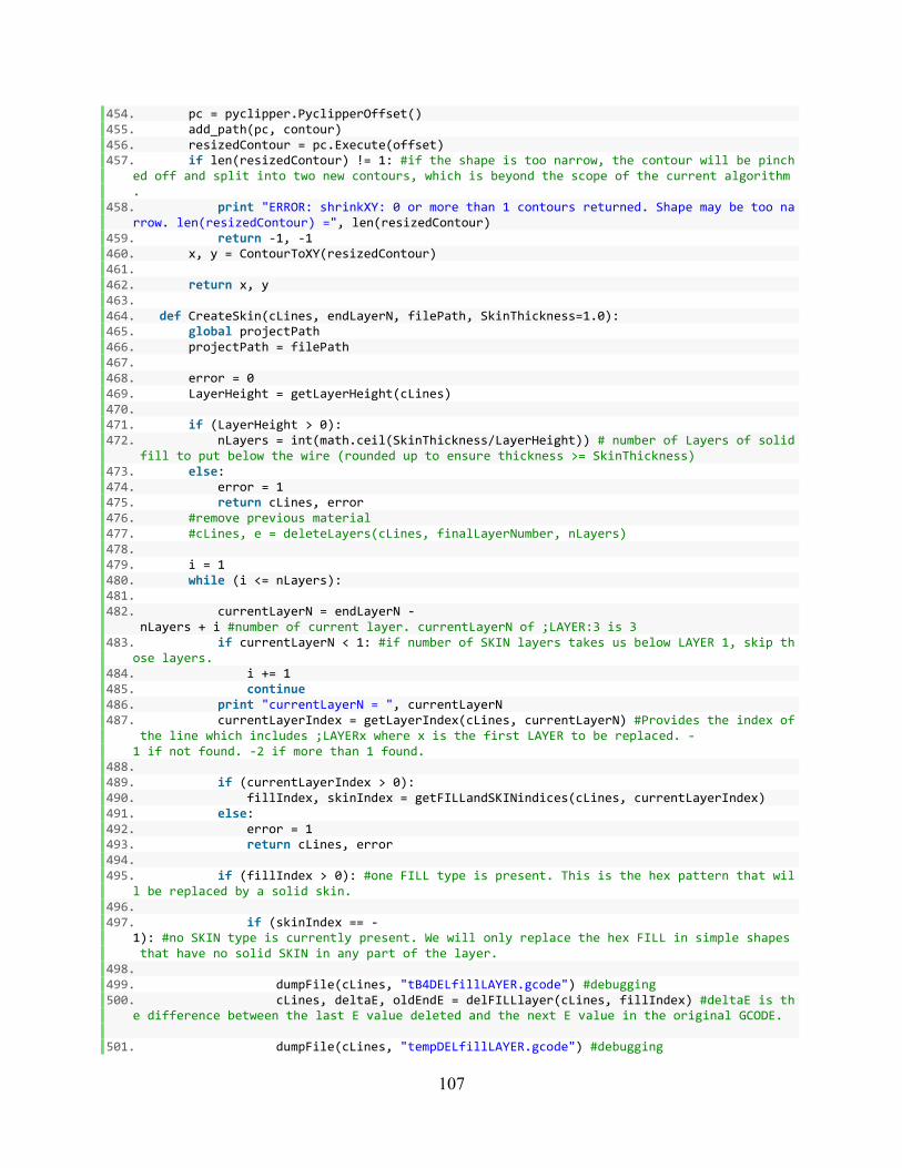
107
454. pc = pyclipper.PyclipperOffset() 455. add_path(pc, contour) 456. resizedContour = pc.Execute(offset) 457. if len(resizedContour) != 1: #if the shape is too narrow, the contour will be pinch
ed off and split into two new contours, which is beyond the scope of the current algorithm.
458. print "ERROR: shrinkXY: 0 or more than 1 contours returned. Shape may be too narrow. len(resizedContour) =", len(resizedContour)
459. return -1, -1 460. x, y = ContourToXY(resizedContour) 461. 462. return x, y 463. 464. def CreateSkin(cLines, endLayerN, filePath, SkinThickness=1.0): 465. global projectPath 466. projectPath = filePath 467. 468. error = 0 469. LayerHeight = getLayerHeight(cLines) 470. 471. if (LayerHeight > 0): 472. nLayers = int(math.ceil(SkinThickness/LayerHeight)) # number of Layers of solid
fill to put below the wire (rounded up to ensure thickness >= SkinThickness) 473. else: 474. error = 1 475. return cLines, error 476. #remove previous material 477. #cLines, e = deleteLayers(cLines, finalLayerNumber, nLayers) 478. 479. i = 1 480. while (i <= nLayers): 481. 482. currentLayerN = endLayerN -
nLayers + i #number of current layer. currentLayerN of ;LAYER:3 is 3 483. if currentLayerN < 1: #if number of SKIN layers takes us below LAYER 1, skip th
ose layers. 484. i += 1 485. continue 486. print "currentLayerN = ", currentLayerN 487. currentLayerIndex = getLayerIndex(cLines, currentLayerN) #Provides the index of
the line which includes ;LAYERx where x is the first LAYER to be replaced. -1 if not found. -2 if more than 1 found.
488. 489. if (currentLayerIndex > 0): 490. fillIndex, skinIndex = getFILLandSKINindices(cLines, currentLayerIndex) 491. else: 492. error = 1 493. return cLines, error 494. 495. if (fillIndex > 0): #one FILL type is present. This is the hex pattern that wil
l be replaced by a solid skin. 496. 497. if (skinIndex == -
1): #no SKIN type is currently present. We will only replace the hex FILL in simple shapes that have no solid SKIN in any part of the layer.
498. 499. dumpFile(cLines, "tB4DELfillLAYER.gcode") #debugging 500. cLines, deltaE, oldEndE = delFILLlayer(cLines, fillIndex) #deltaE is th
e difference between the last E value deleted and the next E value in the original GCODE.
501. dumpFile(cLines, "tempDELfillLAYER.gcode") #debugging
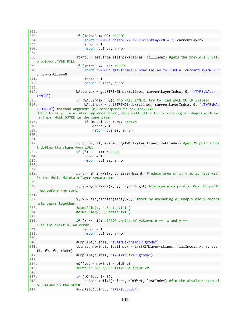
108
502. 503. if (deltaE <= 0): #ERROR 504. print "ERROR: deltaE <= 0. currentLayerN = ", currentLayerN 505. error = 1 506. return cLines, error 507. 508. startE = getEfromFillIndex(cLines, fillIndex) #gets the previous E valu
e before ;TYPE:FILL 509. if (startE == -1): #ERROR 510. print "ERROR: getEfromFillIndex failed to find e. currentLayerN = "
, currentLayerN 511. error = 1 512. return cLines, error 513. 514. WALLindex = getSTRINGindex(cLines, currentLayerIndex, 0, ';TYPE:WALL-
INNER') 515. if (WALLindex < 0): #no WALL_INNER, try to find WALL_OUTER instead 516. WALLindex = getSTRINGindex(cLines, currentLayerIndex, 0, ';TYPE:WAL
L-OUTER') #second argument (0) corresponds to how many WALL-OUTER to skip. In a later implementation, this will allow for processing of shapes with more than WALL_OUTER in the same layer.
517. if (WALLindex < 0): #ERROR 518. error = 1 519. return cLines, error 520. 521. 522. x, y, f0, f1, eRate = getWALLxyfe(cLines, WALLindex) #get XY points tha
t define the shape from WALL 523. if (f1 == -1): #ERROR 524. error = 1 525. return cLines, error 526. 527. 528. x, y = shrinkXY(x, y, LayerHeight) #reduce area of x, y so it fits with
in the WALL. Maintain layer separation 529. 530. x, y = QuantizeY(x, y, LayerHeight) #Interpolates points. Must be perfo
rmed before the sort. 531. 532. y, x = zip(*sorted(zip(y,x))) #sort by ascending y; keep x and y coordi
nate pairs together. 533. #dumpFile(x, "xSorted.txt") 534. #dumpFile(y, "ySorted.txt") 535. 536. if (x == -1): #ERROR shrink XY returns x == -1 and y == -
1 in the event of an error. 537. error = 1 538. return cLines, error 539. 540. dumpFile(cLines, "tB4INSskinLAYER.gcode") 541. cLines, newEndE, lastIndex = insSKINlayer(cLines, fillIndex, x, y, star
tE, f0, f1, eRate) 542. dumpFile(cLines, "INSskinLAYER.gcode") 543. 544. eOffset = newEndE - oldEndE 545. #eOffset can be positive or negative 546. 547. if (eOffset != 0): 548. cLines = fixE(cLines, eOffset, lastIndex) #fix the absolute extrusi
on values in the GCODE 549. dumpFile(cLines, "tFixE.gcode")
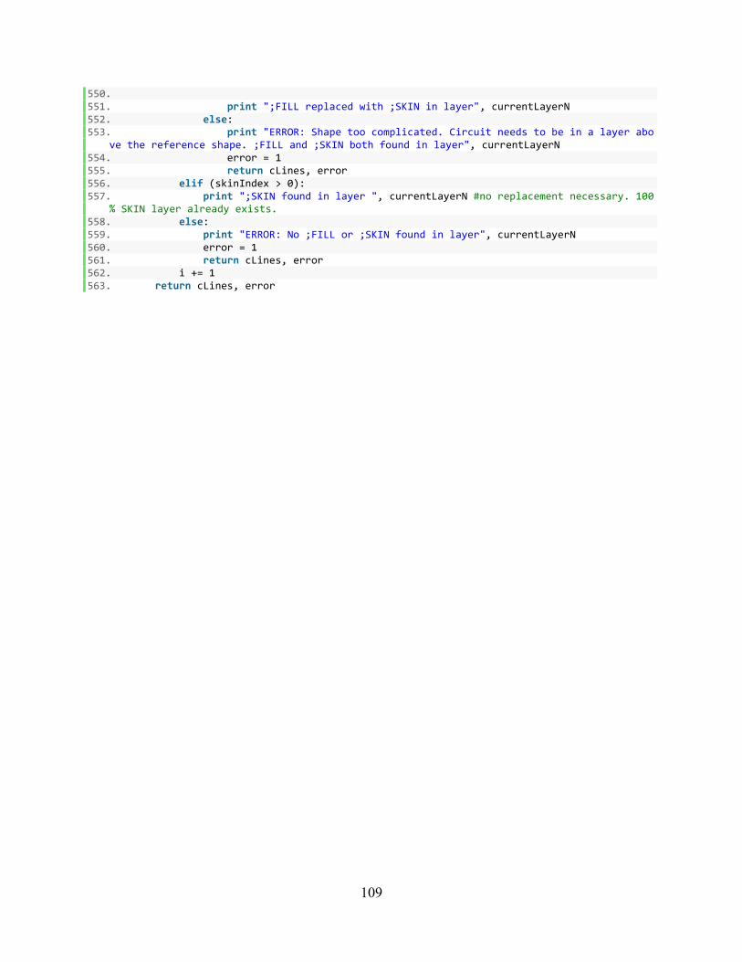
109
550. 551. print ";FILL replaced with ;SKIN in layer", currentLayerN 552. else: 553. print "ERROR: Shape too complicated. Circuit needs to be in a layer abo
ve the reference shape. ;FILL and ;SKIN both found in layer", currentLayerN 554. error = 1 555. return cLines, error 556. elif (skinIndex > 0): 557. print ";SKIN found in layer ", currentLayerN #no replacement necessary. 100
% SKIN layer already exists. 558. else: 559. print "ERROR: No ;FILL or ;SKIN found in layer", currentLayerN 560. error = 1 561. return cLines, error 562. i += 1 563. return cLines, error
110
Vita
The elder of two sons of Peter and Jenny Bailey, Callum Peter Bailey was born in St.
Helier, Jersey, an island in the English Channel. In 2002, after completing his secondary
education at Victoria College, Callum matriculated into Hertford College at the University of
Oxford to read for an undergraduate master’s degree in chemistry. In 2006, he completed his
thesis on Nuclear Magnetic Resonance Structural Investigation of β-Amino Acid Foldamers
which resulted in his attainment of an upper second-class honours degree classification.
After his degree, Callum embarked on a gap year adventure, traveling to Thailand,
Malaysia, Singapore, Australia, New Zealand, the United States, and Canada. During his time in
the US, he met his future wife, Heather, whom he married in 2008 before relocating to Houston,
TX. In Houston, Callum found employment as an industrial R&D chemist, working for the
French multinational oil company, Total. At Total, Callum worked in both the Base Chemicals
and Polymers research departments, where he led the design and construction process of a lab-
scale polystyrene pilot plant. It was during this process that an interest in industrial automation
and 3D printing (in which high-impact polystyrene is a common feedstock) was kindled.
In the summer of 2014, Heather was admitted to medical school at the Paul L. Foster
School of Medicine in El Paso, TX. Taking the opportunity for a career change and to develop
his interests in process automation, Callum enrolled at The University of Texas at El Paso to
study for a master’s degree in electrical engineering. Shortly after arriving, he met 3D-printing
guru, Dr. Eric MacDonald, who inducted him into his research group and the W.M. Keck Center
for 3D Innovation. In the group Callum initially worked on applications for 3D printed parts,
including a project funded by Lockheed Martin to develop 3D printed hinges featuring electrical

111
connections. Later, Callum transferred to developing control programming and the work
described in this publication.
Contact Information: [email protected]
This thesis was typed by Callum Peter Bailey


![The 3D printing ‘revolution’ · 3D printing ‘Bigger than internet’ FT 21.6.12 3D printing: ‘The PC all over again?’ Economist 1.12.12 ‘3D printing [..] has the potential](https://img.pdfslide.net/doc/110x75/5f08eac77e708231d42459a8/the-3d-printing-arevolutiona-3d-printing-abigger-than-interneta-ft-21612.jpg)