G. Cowan Lectures on Statistical Data Analysis Lecture 3 page 1 Lecture 3 1 Probability (90 min.) Definition, Bayes’ theorem, probability densities and

G. Cowan Lectures on Statistical Data Analysis Lecture 3 page 1

Lecture 31 Probability (90 min.)

Definition, Bayes’ theorem, probability densities and their properties, catalogue of pdfs, Monte Carlo

2 Statistical tests (90 min.)general concepts, test statistics, multivariate methods,goodness-of-fit tests

3 Parameter estimation (90 min.)general concepts, maximum likelihood, variance of estimators, least squares

4 Interval estimation (60 min.)setting limits

5 Further topics (60 min.)systematic errors, MCMC


Parameter estimationThe parameters of a pdf are constants that characterize its shape, e.g.

r.v.

Suppose we have a sample of observed values:

parameter

We want to find some function of the data to estimate the parameter(s):

← estimator written with a hat

Sometimes we say ‘estimator’ for the function of x1, ..., xn;‘estimate’ for the value of the estimator with a particular data set.


Properties of estimatorsIf we were to repeat the entire measurement, the estimatesfrom each would follow a pdf:

biasedlargevariance

best

We want small (or zero) bias (systematic error):

→ average of repeated estimates should tend to true value.

And we want a small variance (statistical error):

→ small bias & variance are in general conflicting criteria


An estimator for the mean (expectation value)

Parameter:

Estimator:

We find:

(‘sample mean’)


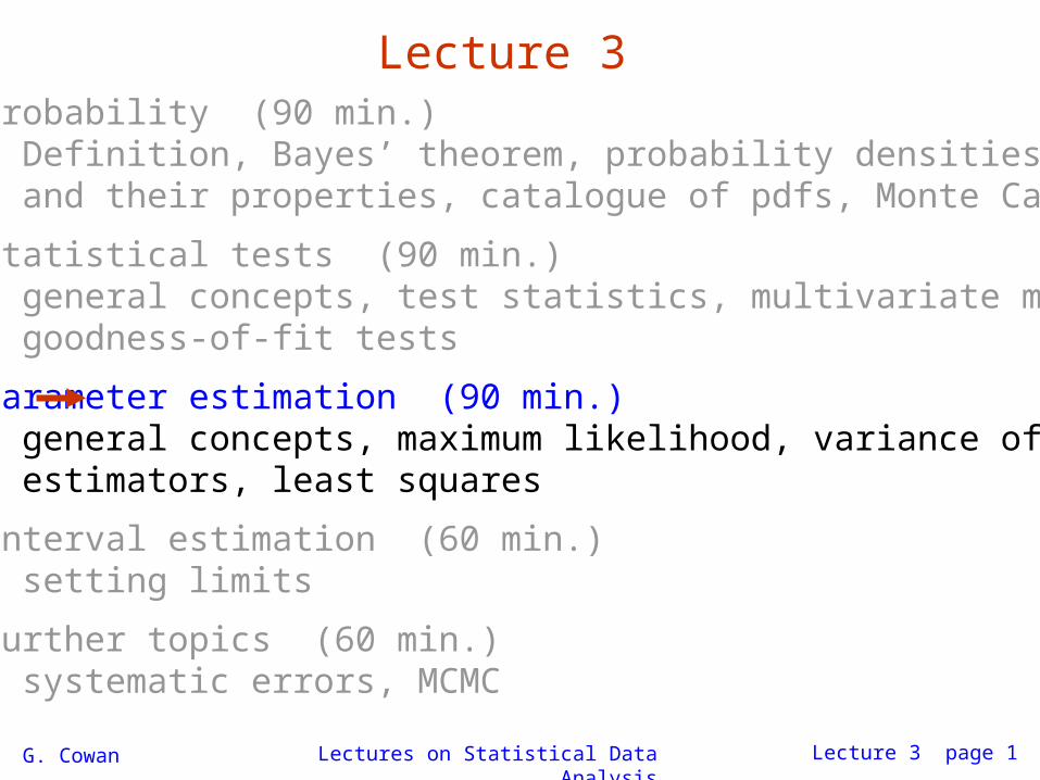
An estimator for the variance

Parameter:

Estimator:

(factor of n1 makes this so)

(‘samplevariance’)

We find:

where


The likelihood function

Consider n independent observations of x: x1, ..., xn, where x follows f (x; ). The joint pdf for the whole data sample is:

Now evaluate this function with the data sample obtained andregard it as a function of the parameter(s). This is the likelihood function:

(xi constant)


Maximum likelihood estimatorsIf the hypothesized is close to the true value, then we expect a high probability to get data like that which we actually found.

So we define the maximum likelihood (ML) estimator(s) to be the parameter value(s) for which the likelihood is maximum.

ML estimators not guaranteed to have any ‘optimal’properties, (but in practice they’re very good).


ML example: parameter of exponential pdf

Consider exponential pdf,

and suppose we have data,

The likelihood function is

The value of for which L() is maximum also gives the maximum value of its logarithm (the log-likelihood function):


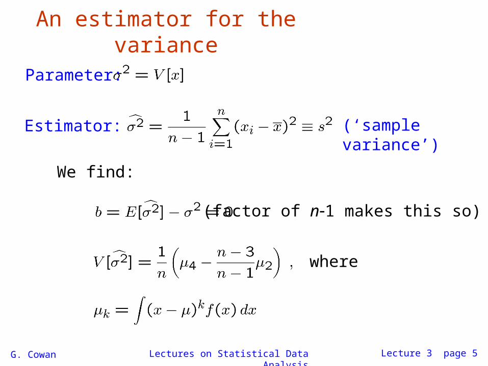
ML example: parameter of exponential pdf (2)

Find its maximum from

→

Monte Carlo test: generate 50 valuesusing = 1:

We find the ML estimate:

(Exercise: show this estimator is unbiased.)


Functions of ML estimators

Suppose we had written the exponential pdf asi.e., we use = 1/. What is the ML estimator for ?

For a function () of a parameter , it doesn’t matterwhether we express L as a function of or .

The ML estimator of a function () is simply

So for the decay constant we have

Caveat: is biased, even though is unbiased.

(bias →0 for n →∞)Can show


Example of ML: parameters of Gaussian pdf

Consider independent x1, ..., xn, with xi ~ Gaussian (,2)

The log-likelihood function is


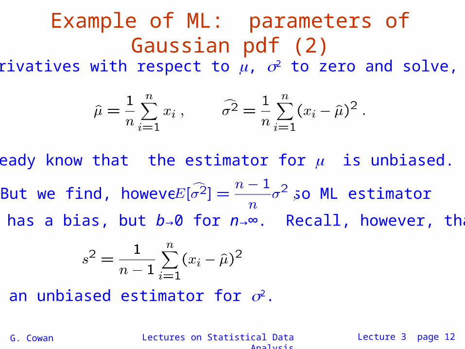
Example of ML: parameters of Gaussian pdf (2)

Set derivatives with respect to , 2 to zero and solve,

We already know that the estimator for is unbiased.

But we find, however, so ML estimator

for 2 has a bias, but b→0 for n→∞. Recall, however, that

is an unbiased estimator for 2.


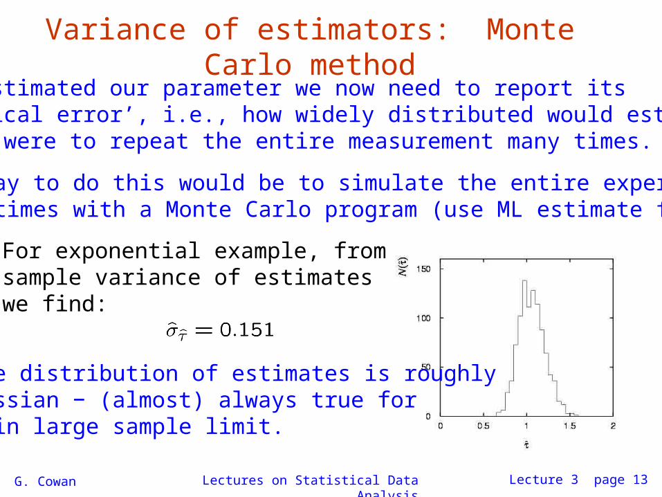
Variance of estimators: Monte Carlo methodHaving estimated our parameter we now need to report its‘statistical error’, i.e., how widely distributed would estimatesbe if we were to repeat the entire measurement many times.

One way to do this would be to simulate the entire experimentmany times with a Monte Carlo program (use ML estimate for MC).

For exponential example, from sample variance of estimateswe find:

Note distribution of estimates is roughlyGaussian − (almost) always true for ML in large sample limit.


Variance of estimators from information inequalityThe information inequality (RCF) sets a minimum variance bound (MVB) for any estimator (not only ML):

Often the bias b is small, and equality either holds exactly oris a good approximation (e.g. large data sample limit). Then,

Estimate this using the 2nd derivative of ln L at its maximum:


Variance of estimators: graphical methodExpand ln L () about its maximum:

First term is ln Lmax, second term is zero, for third term use information inequality (assume equality):

i.e.,

→ to get , change away from until ln L decreases by 1/2.


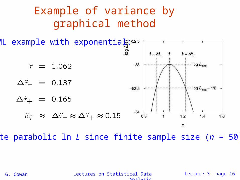
Example of variance by graphical method

ML example with exponential:

Not quite parabolic ln L since finite sample size (n = 50).


Information inequality for n parametersSuppose we have estimated n parameters

The (inverse) minimum variance bound is given by the Fisher information matrix:

The information inequality then states that V I is a positivesemi-definite matrix; therefore for the diagonal elements,

Often use I as an approximation for covariance matrix, estimate using e.g. matrix of 2nd derivatives at maximum of L.


Example of ML with 2 parameters

Consider a scattering angle distribution with x = cos ,

or if xmin < x < xmax, need always to normalize so that

Example: = 0.5, = 0.5, xmin = 0.95, xmax = 0.95, generate n = 2000 events with Monte Carlo.


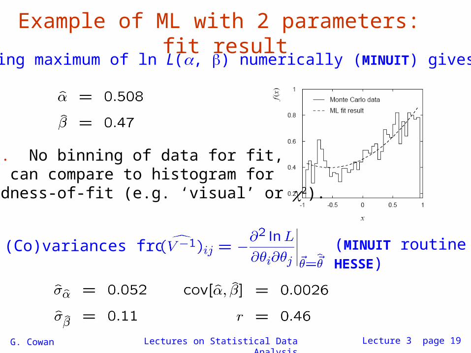
Example of ML with 2 parameters: fit resultFinding maximum of ln L(, ) numerically (MINUIT) gives

N.B. No binning of data for fit,but can compare to histogram forgoodness-of-fit (e.g. ‘visual’ or 2).

(Co)variances from (MINUIT routine HESSE)


Two-parameter fit: MC studyRepeat ML fit with 500 experiments, all with n = 2000 events:

Estimates average to ~ true values;(Co)variances close to previous estimates;marginal pdfs approximately Gaussian.


The ln Lmax 1/2 contour

For large n, ln L takes on quadratic form near maximum:

The contour is an ellipse:


(Co)variances from ln L contour

→ Tangent lines to contours give standard deviations.

→ Angle of ellipse related to correlation:

Correlations between estimators result in an increasein their standard deviations (statistical errors).

The , plane for the firstMC data set


Extended MLSometimes regard n not as fixed, but as a Poisson r.v., mean .

Result of experiment defined as: n, x1, ..., xn.

The (extended) likelihood function is:

Suppose theory gives = (), then the log-likelihood is

where C represents terms not depending on .


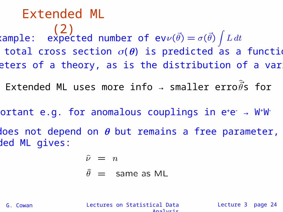
Extended ML (2)

Extended ML uses more info → smaller errors for

Example: expected number of events

where the total cross section () is predicted as a function of

the parameters of a theory, as is the distribution of a variable x.

If does not depend on but remains a free parameter,extended ML gives:

Important e.g. for anomalous couplings in ee → W+W


Extended ML exampleConsider two types of events (e.g., signal and background) each of which predict a given pdf for the variable x: fs(x) and fb(x).

We observe a mixture of the two event types, signal fraction = , expected total number = , observed total number = n.

Let goal is to estimate s, b.

→


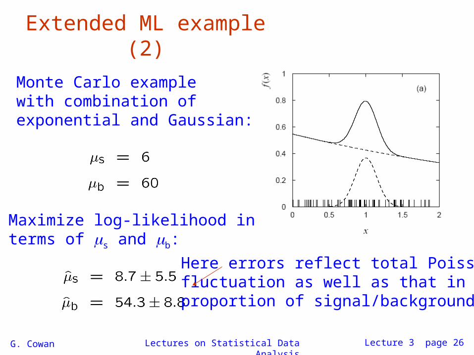
Extended ML example (2)

Maximize log-likelihood in terms of s and b:

Monte Carlo examplewith combination ofexponential and Gaussian:

Here errors reflect total Poissonfluctuation as well as that in proportion of signal/background.


Extended ML example: an unphysical estimate

A downwards fluctuation of data in the peak region can leadto even fewer events than what would be obtained frombackground alone.

Estimate for s here pushednegative (unphysical).

We can let this happen as long as the (total) pdf stayspositive everywhere.


Unphysical estimators (2)

Here the unphysical estimator is unbiased and should nevertheless be reported, since average of a large number of unbiased estimates converges to the true value (cf. PDG).

Repeat entire MCexperiment many times, allow unphysical estimates:


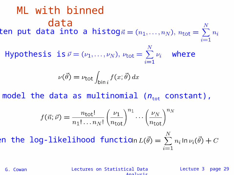
ML with binned dataOften put data into a histogram:

Hypothesis is where

If we model the data as multinomial (ntot constant),

then the log-likelihood function is:


ML example with binned dataPrevious example with exponential, now put data into histogram:

Limit of zero bin width → usual unbinned ML.

If ni treated as Poisson, we get extended log-likelihood:


Relationship between ML and Bayesian estimators

In Bayesian statistics, both and x are random variables:

Recall the Bayesian method:

Use subjective probability for hypotheses ();

before experiment, knowledge summarized by prior pdf ();

use Bayes’ theorem to update prior in light of data:

Posterior pdf (conditional pdf for given x)


ML and Bayesian estimators (2)Purist Bayesian: p(| x) contains all knowledge about .

Pragmatist Bayesian: p(| x) could be a complicated function,

→ summarize using an estimator

Take mode of p(| x) , (could also use e.g. expectation value)

What do we use for ()? No golden rule (subjective!), oftenrepresent ‘prior ignorance’ by () = constant, in which case

But... we could have used a different parameter, e.g., = 1/,and if prior () is constant, then () is not!

‘Complete prior ignorance’ is not well defined.


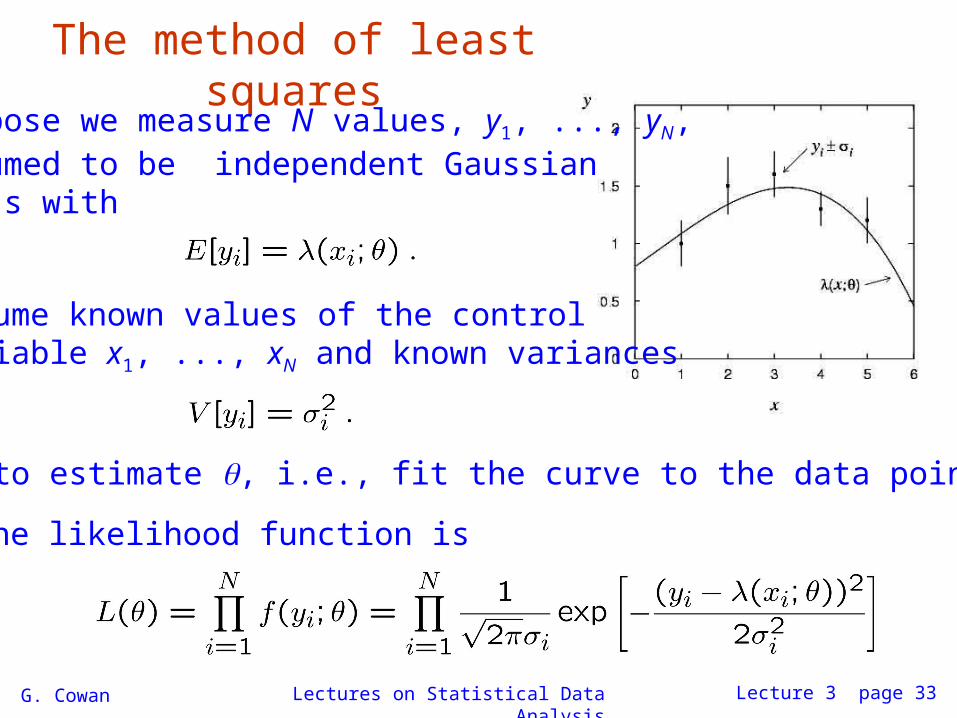
The method of least squaresSuppose we measure N values, y1, ..., yN, assumed to be independent Gaussian r.v.s with

Assume known values of the controlvariable x1, ..., xN and known variances

The likelihood function is

We want to estimate , i.e., fit the curve to the data points.


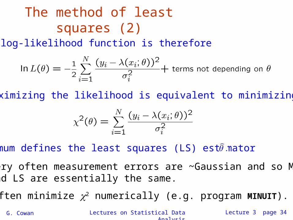
The method of least squares (2)

The log-likelihood function is therefore

So maximizing the likelihood is equivalent to minimizing

Minimum defines the least squares (LS) estimator

Very often measurement errors are ~Gaussian and so MLand LS are essentially the same.

Often minimize 2 numerically (e.g. program MINUIT).


LS with correlated measurements

If the yi follow a multivariate Gaussian, covariance matrix V,

Then maximizing the likelihood is equivalent to minimizing


Example of least squares fit

Fit a polynomial of order p:


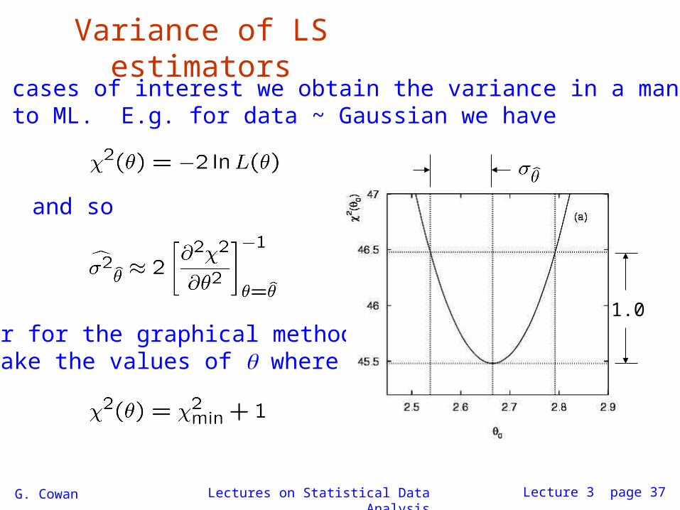
Variance of LS estimatorsIn most cases of interest we obtain the variance in a mannersimilar to ML. E.g. for data ~ Gaussian we have

and so

or for the graphical method we take the values of where

1.0


Two-parameter LS fit


Goodness-of-fit with least squaresThe value of the 2 at its minimum is a measure of the levelof agreement between the data and fitted curve:

It can therefore be employed as a goodness-of-fit statistic totest the hypothesized functional form (x; ).

We can show that if the hypothesis is correct, then the statistic t = 2

min follows the chi-square pdf,

where the number of degrees of freedom is

nd = number of data points number of fitted parameters


Goodness-of-fit with least squares (2)

The chi-square pdf has an expectation value equal to the number of degrees of freedom, so if 2

min ≈ nd the fit is ‘good’.

More generally, find the p-value:

E.g. for the previous example with 1st order polynomial (line),

whereas for the 0th order polynomial (horizontal line),

This is the probability of obtaining a 2min as high as the one

we got, or higher, if the hypothesis is correct.


Wrapping up lecture 3

No golden rule for parameter estimation, construct so as to havedesirable properties (small variance, small or zero bias, ...)

Most important methods:Maximum Likelihood,Least Squares

Several methods to obtain variances (stat. errors) from a fitAnalyticallyMonte CarloFrom information equality / graphical method

Finding estimator often involves numerical minimization


Extra slides for lecture 3

Goodness-of-fit vs. statistical errors

Fitting histograms with LS

Combining measurements with LS


Goodness-of-fit vs. statistical errors


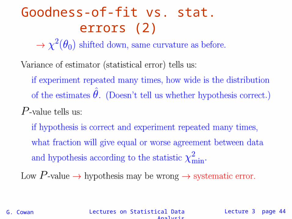
Goodness-of-fit vs. stat. errors (2)


LS with binned data


LS with binned data (2)


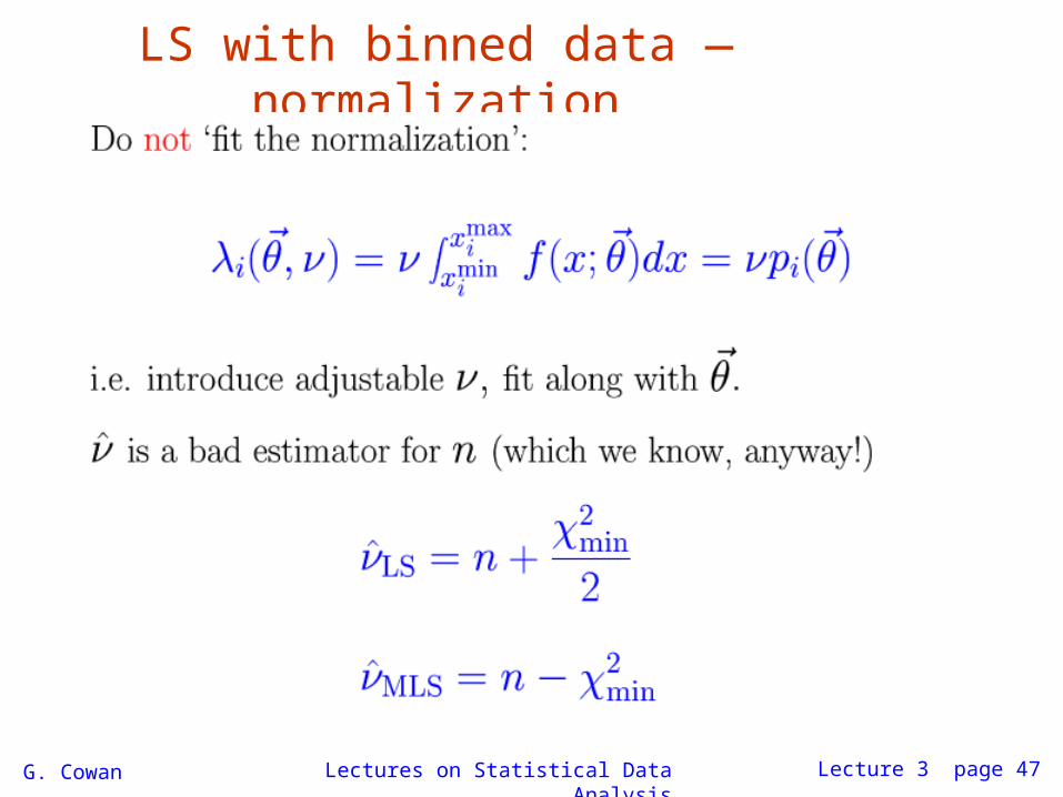
LS with binned data — normalization


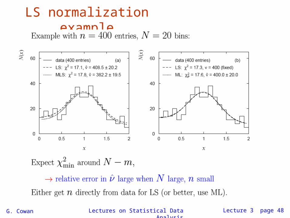
LS normalization example


Using LS to combine measurements


Combining correlated measurements with LS


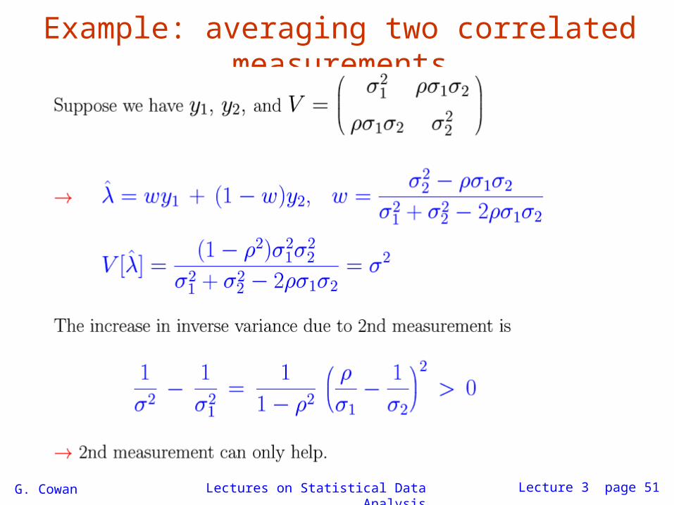
Example: averaging two correlated measurements


Negative weights in LS average

Documents

G. Cowan Lectures on Statistical Data Analysis Lecture 3 page 1 Lecture 3 1 Probability (90 min.) Definition, Bayes’ theorem, probability densities and