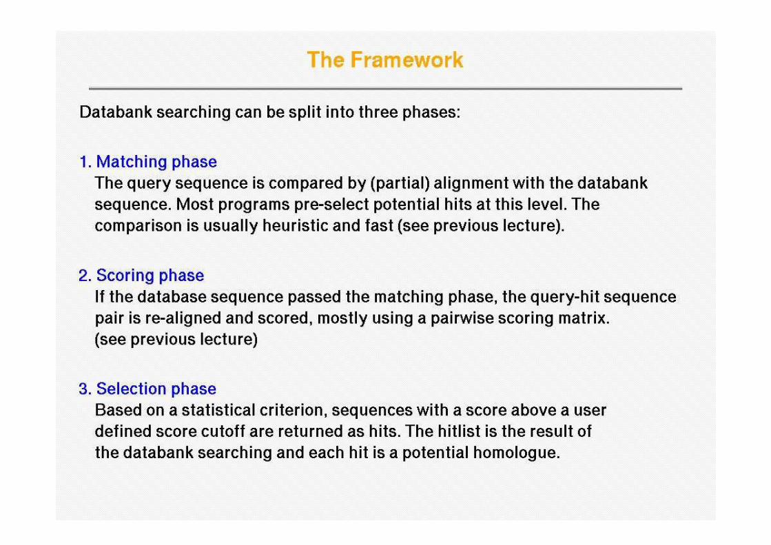
Iterative homology searching

Introduction to bioinformatics 2008

Lecture 10

CENTR

FORINTE

BIOINFO

E

Iterative homology searching using PSI-BLAST, scoring statistics and performance

evaluation

EGRATIVE

ORMATICSVU

Today:•PSI-BLAST

•Statistical scoring of database hits

•Performance evaluation using standard of truth•Performance evaluation using standard of truth

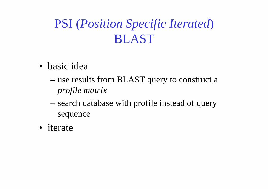
PSI (Position Specific Iterated) BLAST

• basic idea– use results from BLAST query to construct a

profile matrixprofile matrix

– search database with profile instead of query sequence

• iterate

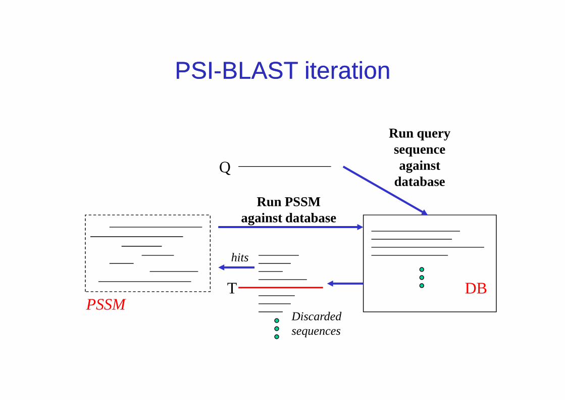
Q

Run query sequence against

database

Run PSSM

PSIPSI--BLAST iterationBLAST iteration

DBT

hits

PSSMDiscarded sequences

Run PSSM against database

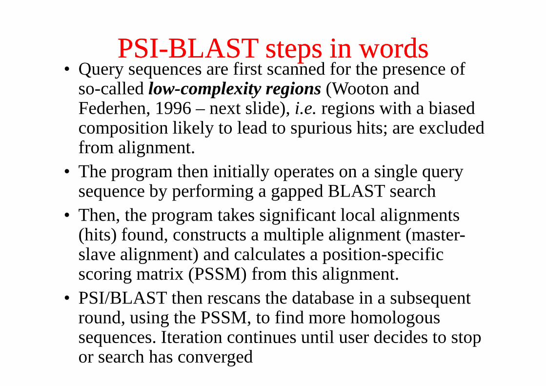
PSI-BLAST steps in words• Query sequences are first scanned for the presence of

so-called low-complexity regions (Wooton and Federhen, 1996 – next slide), i.e. regions with a biased composition likely to lead to spurious hits; are excluded from alignment.

• The program then initially operates on a single query sequence by performing a gapped BLAST search

PSI-BLAST steps in words

sequence by performing a gapped BLAST search• Then, the program takes significant local alignments

(hits) found, constructs a multiple alignment (master-slave alignment) and calculates a position-specific scoring matrix (PSSM) from this alignment.

• PSI/BLAST then rescans the database in a subsequent round, using the PSSM, to find more homologous sequences. Iteration continues until user decides to stop or search has converged

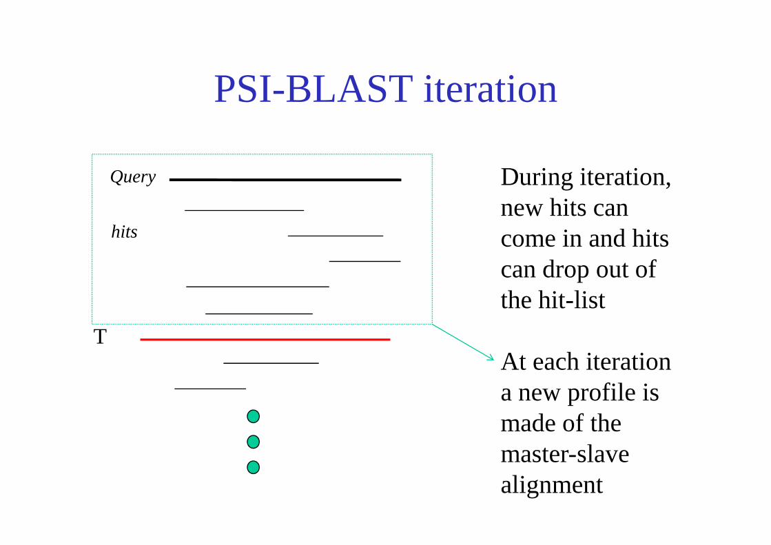
PSI-BLAST iteration

hits

Query During iteration,new hits can come in and hits can drop out of

T

can drop out of the hit-list

At each iteration a new profile is made of the master-slave alignment

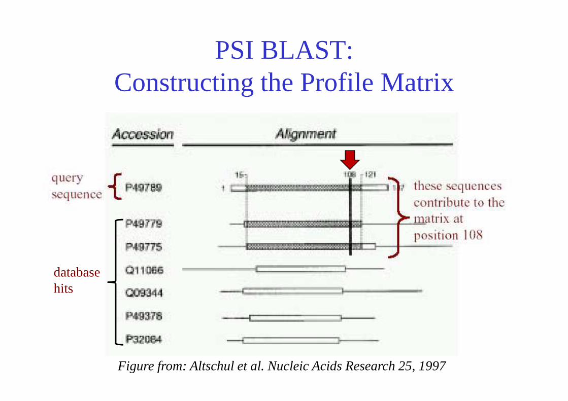
PSI BLAST:Constructing the Profile Matrix

Figure from: Altschul et al. Nucleic Acids Research 25, 1997

database hits

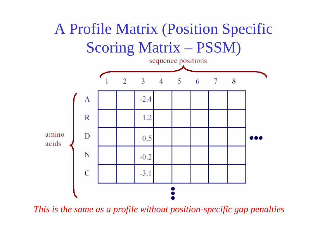
A Profile Matrix (Position Specific Scoring Matrix – PSSM)

This is the same as a profile without position-specific gap penalties

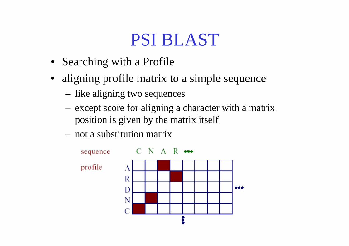
PSI BLAST• Searching with a Profile

• aligning profile matrix to a simple sequence– like aligning two sequences

– except score for aligning a character with a matrix position is given by the matrix itselfposition is given by the matrix itself

– not a substitution matrix

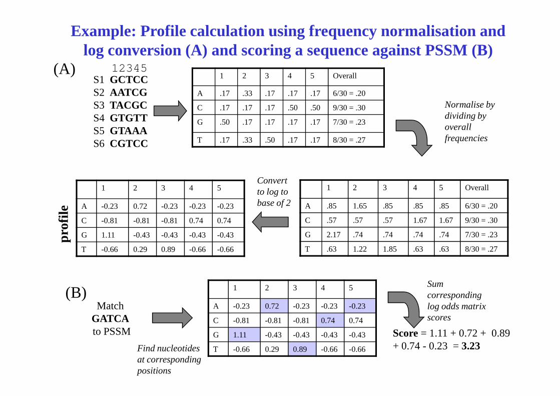
1 2 3 4 5 Overall

A .17 .33 .17 .17 .17 6/30 = .20

C .17 .17 .17 .50 .50 9/30 = .30

G .50 .17 .17 .17 .17 7/30 = .23

T .17 .33 .50 .17 .17 8/30 = .27

S1 GCTCCS2 AATCGS3 TACGCS4 GTGTTS5 GTAAAS6 CGTCC

1 2 3 4 5 Overall1 2 3 4 5

Normalise by dividing by overall frequencies

Convert to log to base of 2

(A)

Example: Profile calculation using frequency normalisation and log conversion (A) and scoring a sequence against PSSM (B)

12345

A .85 1.65 .85 .85 .85 6/30 = .20

C .57 .57 .57 1.67 1.67 9/30 = .30

G 2.17 .74 .74 .74 .74 7/30 = .23

T .63 1.22 1.85 .63 .63 8/30 = .27

A -0.23 0.72 -0.23 -0.23 -0.23

C -0.81 -0.81 -0.81 0.74 0.74

G 1.11 -0.43 -0.43 -0.43 -0.43

T -0.66 0.29 0.89 -0.66 -0.66

base of 2

1 2 3 4 5

A -0.23 0.72 -0.23 -0.23 -0.23

C -0.81 -0.81 -0.81 0.74 0.74

G 1.11 -0.43 -0.43 -0.43 -0.43

T -0.66 0.29 0.89 -0.66 -0.66

Match GATCAto PSSM Score = 1.11 + 0.72 + 0.89

+ 0.74 - 0.23 = 3.23Find nucleotides at corresponding positions

Sum corresponding log odds matrix scores

(B)

prof

ile

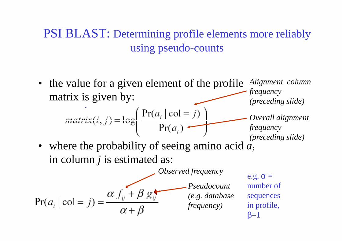
PSI BLAST: Determining profile elements more reliably using pseudo-counts

• the value for a given element of the profile matrix is given by:

Overall alignment

Alignment column frequency (preceding slide)

• where the probability of seeing amino acid ai

in column j is estimated as:Observed frequency

Pseudocount (e.g. database frequency)

e.g. α = number of sequences in profile, β=1

Overall alignment frequency (preceding slide)

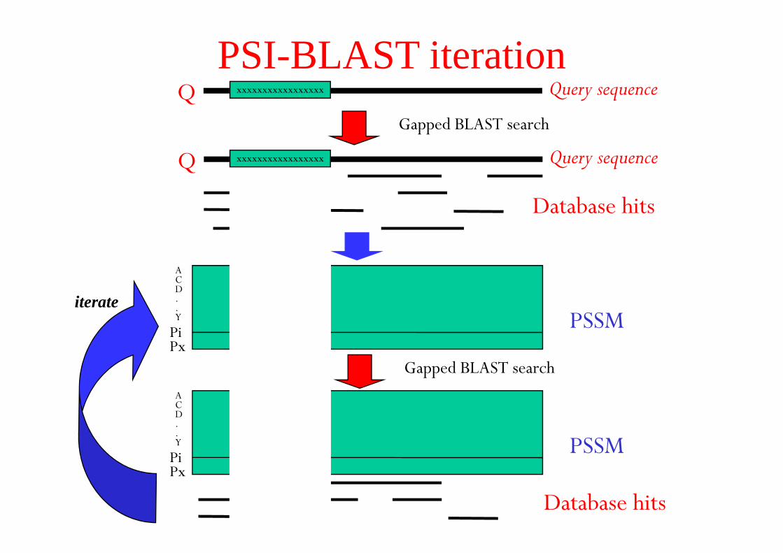
PSI-BLAST iteration

�

��

������������

� ������������

��������� ������

������������

�����������������

�����������������

������

����

����

��������� ������

������

����

����

������������

iterate

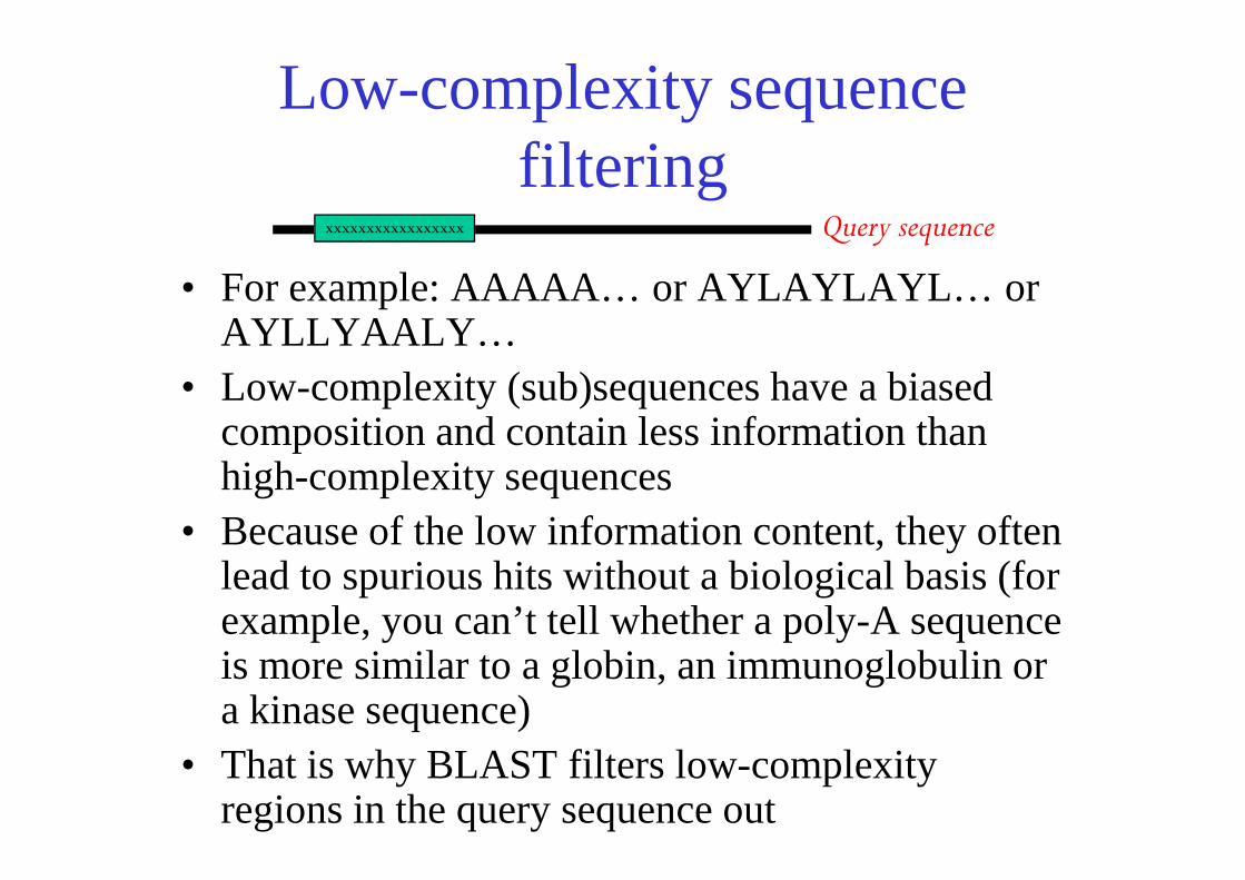
Low-complexity sequence filtering

• For example: AAAAA… or AYLAYLAYL… or AYLLYAALY…

• Low-complexity (sub)sequences have a biased composition and contain less information than

�����������������������������

composition and contain less information than high-complexity sequences

• Because of the low information content, they often lead to spurious hits without a biological basis (for example, you can’ t tell whether a poly-A sequence is more similar to a globin, an immunoglobulin or a kinase sequence)

• That is why BLAST filters low-complexity regions in the query sequence out

The innovation and power of BLAST is the statistical scoring

system• (PSI-)BLAST converts raw alignment scores

based on the – (query-database) sequence lengths– the size of the data base– the (amino acid or nucleotide) composition of the – the (amino acid or nucleotide) composition of the

database

• It also checks to what extend a hit score is higher than randomly expected– BLAST has a clever and fast way for this

• This makes the scores really comparable, so that the hit list can be ordered based on their statistical scores (bit-scores and E-values)

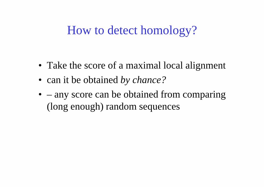
How to detect homology?

• Take the score of a maximal local alignment

• can it be obtained by chance?

• – any score can be obtained from comparing • – any score can be obtained from comparing (long enough) random sequences

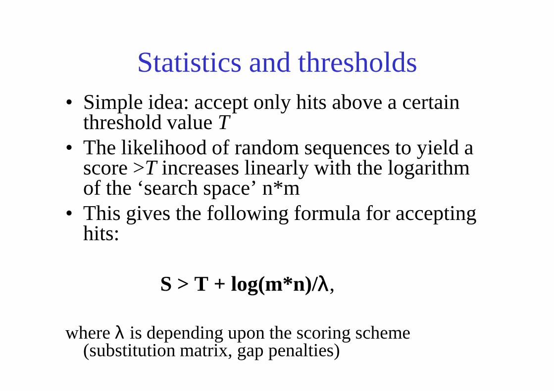
Statistics and thresholds• Simple idea: accept only hits above a certain

threshold value T• The likelihood of random sequences to yield a

score >T increases linearly with the logarithm of the ‘search space’ n*mof the ‘search space’ n*m

• This gives the following formula for accepting hits:

S > T + log(m*n)/λλλλ,

where λ is depending upon the scoring scheme (substitution matrix, gap penalties)

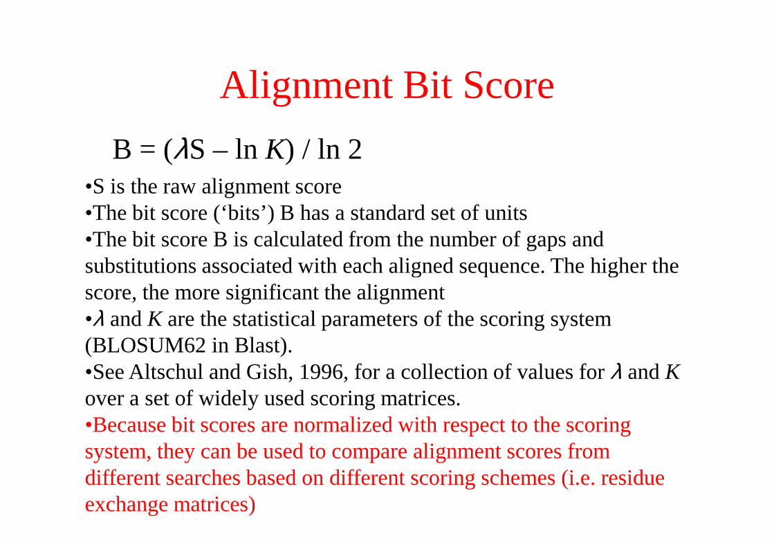
Alignment Bit Score

•S is the raw alignment score •The bit score (‘bits’ ) B has a standard set of units•The bit score B iscalculated from the number of gaps and substitutions associated with each aligned sequence. The higher the

B = (λS – ln K) / ln 2

substitutions associated with each aligned sequence. The higher the score, the more significant the alignment •λ and K are the statistical parameters of the scoring system(BLOSUM62 in Blast). •See Altschul and Gish, 1996, for a collection of values for λ and Kover a set of widely used scoring matrices.•Because bit scores arenormalized with respect to the scoring system, they can be used to compare alignment scores from different searchesbased on different scoring schemes (i.e. residue exchange matrices)

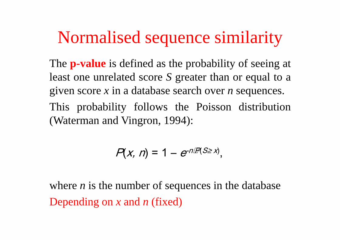
Normalised sequence similarityThe p-value is defined as the probability of seeing atleast one unrelated score S greater than or equal to agiven scorex in a databasesearch over n sequences.

This probability follows the Poisson distribution(Waterman and Vingron, 1994):(Waterman and Vingron, 1994):

⋅ ≥

wheren is thenumber of sequences in thedatabase

Depending on x and n (fixed)

Normalised sequence similarityStatistical significance

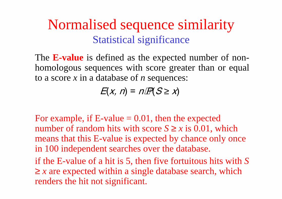
The E-value is defined as the expected number of non-homologous sequences with score greater than or equalto ascorex in a databaseof n sequences:

⋅ ≥

For example, if E-value = 0.01, then the expected number of random hits with score S≥ x is 0.01, which means that this E-value is expected by chance only once in 100 independent searches over the database.if the E-value of a hit is 5, then five fortuitous hits with S ≥ x are expected within a single database search, which renders the hit not significant.

A model for database searching score probabilities

• Scores resulting from searching with a query sequence against a database follow the Extreme Value Distribution (EDV) the Extreme Value Distribution (EDV) (Gumbel, 1955).

• Using the EDV, the raw alignment scores are converted to a statistical score (E value) that keeps track of the database amino acid composition and the scoring scheme (a.a. exchange matrix)

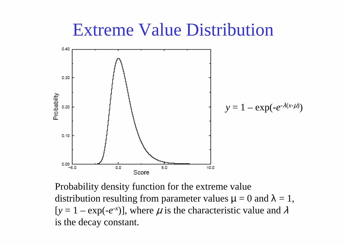
Extreme Value Distribution

y = 1 – exp(-e-λ(x-µ))

Probability density function for the extreme value distribution resulting from parameter values µ = 0 and λ = 1, [y = 1 – exp(-e-x)], where µ is the characteristic value and λis the decay constant.

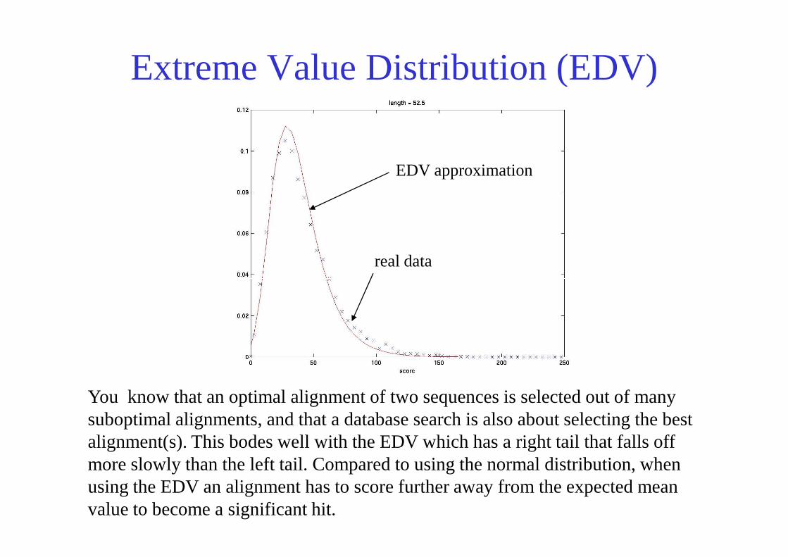
Extreme Value Distribution (EDV)

real data

EDV approximation

You know that an optimal alignment of two sequences is selected out of many suboptimal alignments, and that a database search is also about selecting the best alignment(s). This bodes well with the EDV which has a right tail that falls off more slowly than the left tail. Compared to using the normal distribution, when using the EDV an alignment has to score further away from the expected mean value to become a significant hit.

Extreme Value Distribution

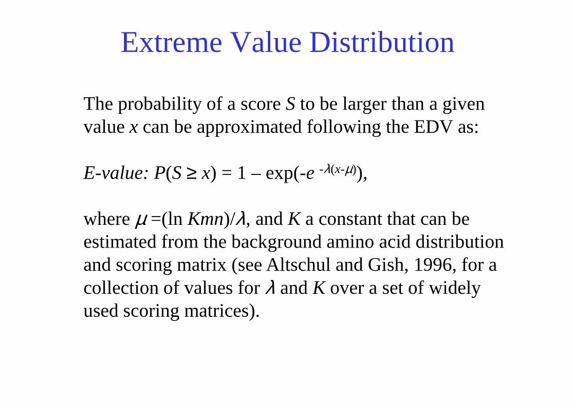
The probability of a score S to be larger than a given value x can be approximated following the EDV as:

E-value: P(S ≥ x) = 1 – exp(-e -λ(x-µ)),

where µ =(ln Kmn)/λ, and K a constant that can be estimated from the background amino acid distribution and scoring matrix (see Altschul and Gish, 1996, for a collection of values for λ and K over a set of widely used scoring matrices).

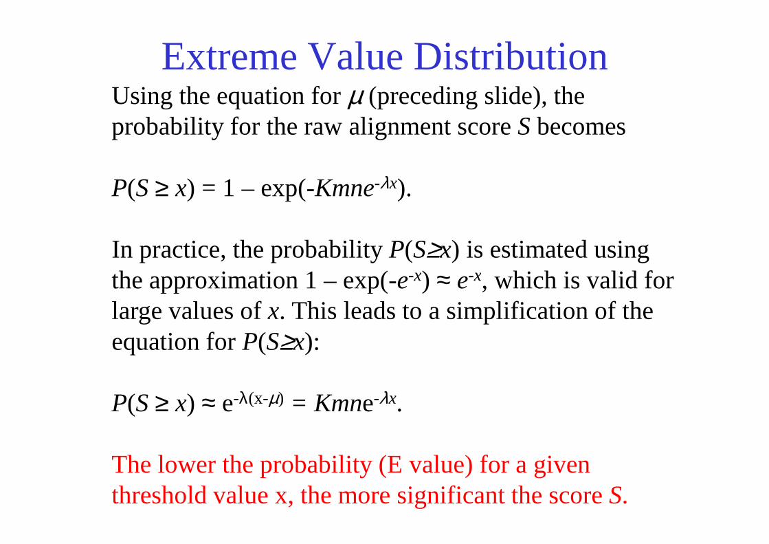
Extreme Value DistributionUsing the equation for µ (preceding slide), the probability for the raw alignment score Sbecomes

P(S ≥ x) = 1 – exp(-Kmne-λx).

In practice, the probability P(S≥x) is estimated using the approximation 1 – exp(-e-x) ≈ e-x, which is valid for the approximation 1 – exp(-e-x) ≈ e-x, which is valid for large values of x. This leads to a simplification of the equation for P(S≥x):

P(S ≥ x) ≈ e-λ(x-µ) = Kmne-λx.

The lower the probability (E value) for a given threshold value x, the more significant the score S.

Normalised sequence similarityStatistical significance

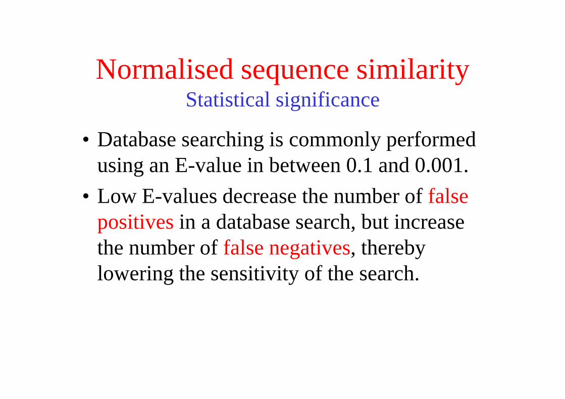
• Database searching is commonly performed using an E-value in between 0.1 and 0.001.

• Low E-values decrease the number of false • Low E-values decrease the number of false positives in a database search, but increase the number of false negatives, thereby lowering the sensitivity of the search.

Words of Encouragement

• “ There are three kinds of lies: lies, damned lies, and statistics” – Benjamin Disraeli

• “ Statistics in the hands of an engineer are like a lamppost to a drunk – they’ re used

• “ Statistics in the hands of an engineer are like a lamppost to a drunk – they’ re used more for support than illumination”

• “ Then there is the man who drowned crossing a stream with an average depth of six inches.” – W.I.E. Gates

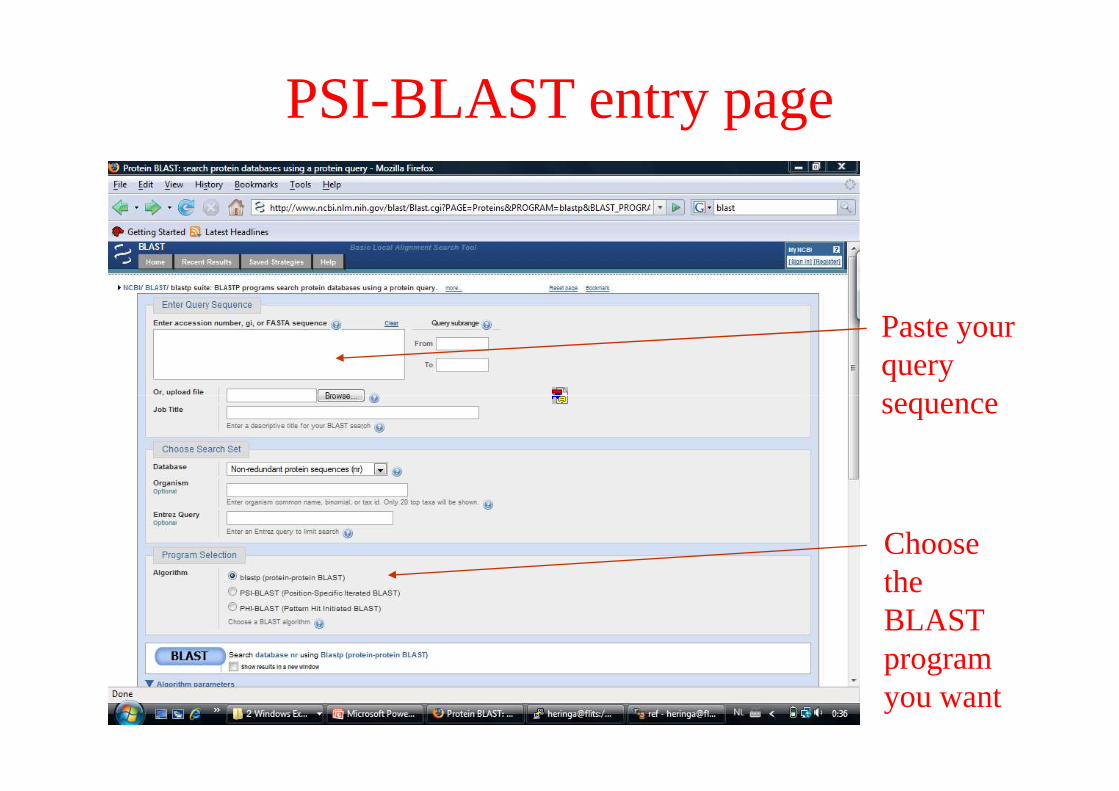
PSI-BLAST entry page

Paste your query sequencesequence

Choose the BLAST program you want

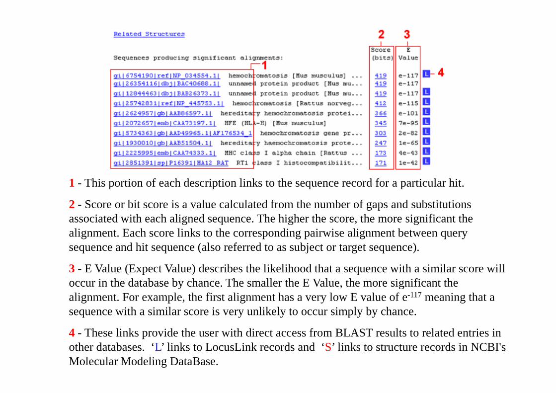
1 - This portion of each description links to the sequence record for a particular hit.

2 - Score or bit score is a value calculated from the number of gaps and substitutions associated with each aligned sequence. The higher the score, the more significant the alignment. Each score links to the corresponding pairwise alignment between query sequence and hit sequence (also referred to as subject or target sequence).

3 - E Value (Expect Value) describes the likelihood that a sequence with a similar score will occur in the database by chance. The smaller the E Value, the more significant the alignment. For example, the first alignment has a very low E value of e-117 meaning that a sequence with a similar score is very unlikely to occur simply by chance.

4 - These links provide the user with direct access from BLAST results to related entries in other databases. ‘L’ links to LocusLink records and ‘S’ links to structure records in NCBI's Molecular Modeling DataBase.

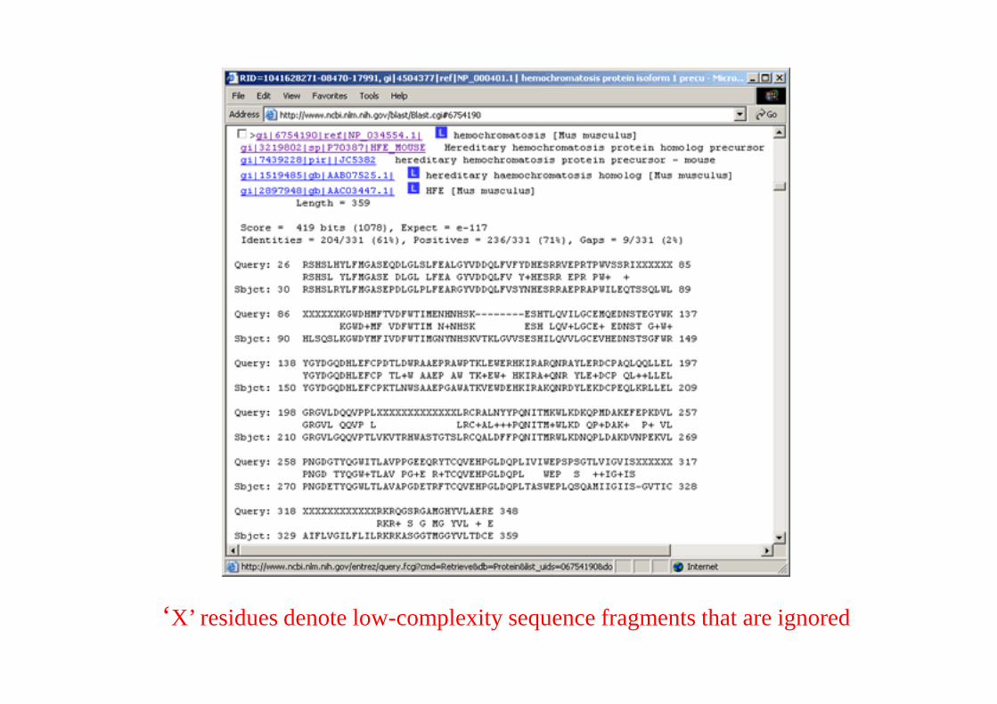
‘X’ residues denote low-complexity sequence fragments that are ignored

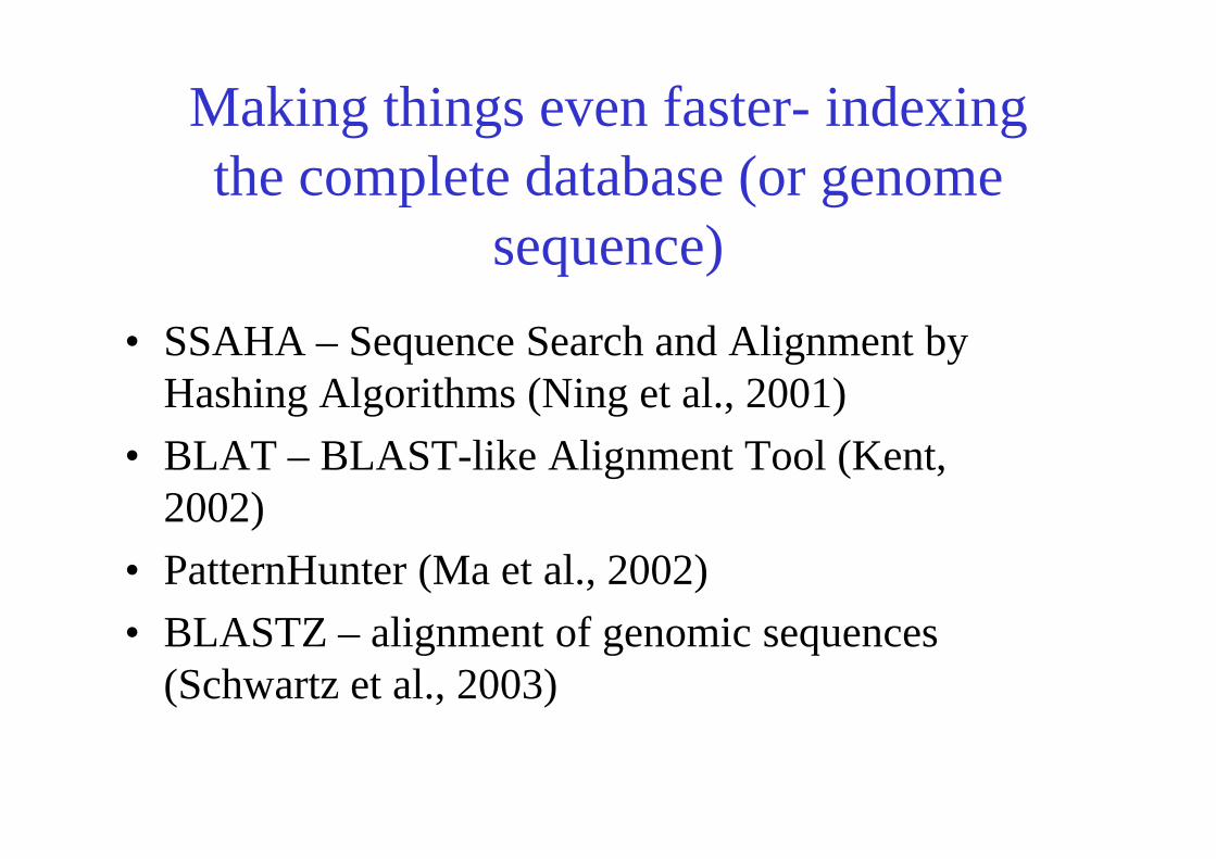
Making things even faster- indexing the complete database (or genome

sequence)

• SSAHA – Sequence Search and Alignment by Hashing Algorithms (Ning et al., 2001)

• BLAT – BLAST-like Alignment Tool (Kent, 2002)

• PatternHunter (Ma et al., 2002)

• BLASTZ – alignment of genomic sequences (Schwartz et al., 2003)

BLAT – BLAST-Like Alignment Tool

• Analyzing vertebrate genomes requires rapid mRNA/DNA and cross-species protein alignments. BLAT (the BLAST-like alignment tool) was developed by Jim Kent from UCSC. It is more accurate and 500 times faster than popular existing tools such as BLAST for mRNA/DNA alignments and 50 times faster for protein alignments at sensitivity settings alignments and 50 times faster for protein alignments at sensitivity settings typically used when comparing vertebrate sequences (e.g. BLAST).

• BLAT's speed stems from an index of all nonoverlapping k-mers in the genome. This index fits inside the RAM of inexpensive computers, and need only be computed once for each genome assembly. BLAT has several major stages. It uses the index to find regions in the genome likely to be homologous to the query sequence. It performs an alignment between homologous regions. It stitches together these aligned regions (often exons) into larger alignments (typically genes). Finally, BLAT revisits small internal exons possibly missed at the first stage and adjusts large gap boundaries that have canonical splice sites where feasible.

• From Wikipedia, the free encyclopedia

Indexing (hashing) the database

• BLAT - The Blast-Like Alignment Tool

• For large-scale genome comparison

– query can be as large as a complete genome– query can be as large as a complete genome

Preprocessing phase:

- BLAST: indexes only the query sequence

- BLAT: indexes the complete database

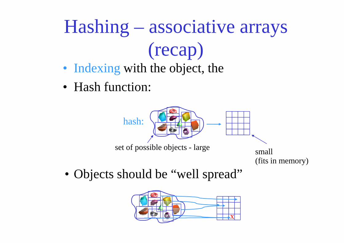
Hashing – associative arrays (recap)

• Indexing with the object, the

• Hash function:

hash:

• Objects should be “well spread”

hash:

x

set of possible objects - large small (fits in memory)

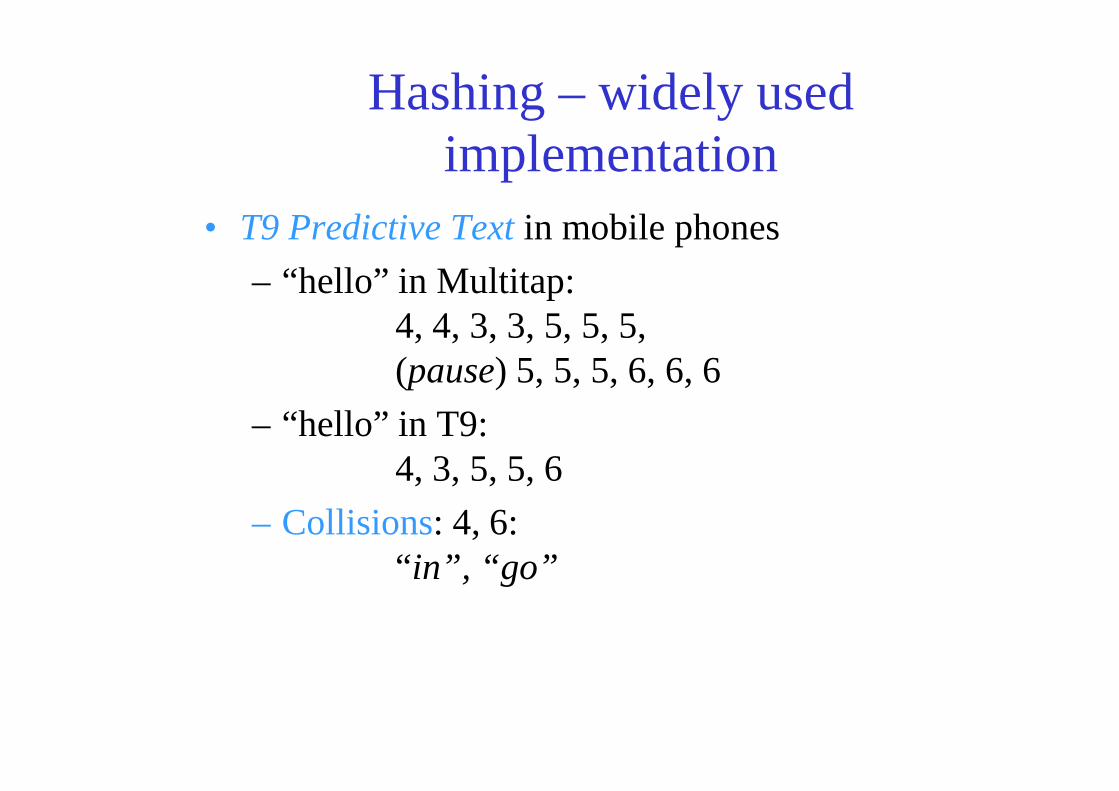
Hashing – widely used implementation

• T9 Predictive Text in mobile phones

– “hello” in Multitap:4, 4, 3, 3, 5, 5, 5, (pause) 5, 5, 5, 6, 6, 6

– “hello” in T9: 4, 3, 5, 5, 6

– Collisions: 4, 6:“ in” , “ go”

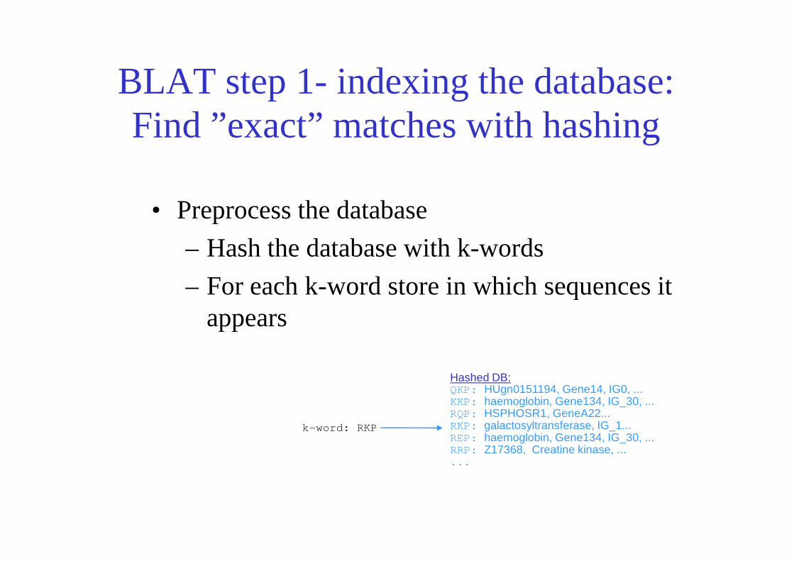
BLAT step 1- indexing the database: Find ”exact” matches with hashing

• Preprocess the database

– Hash the database with k-words

– For each k-word store in which sequences it – For each k-word store in which sequences it appears

k-word: RKP

Hashed DB:QKP: HUgn0151194, Gene14, IG0, ...KKP: haemoglobin, Gene134, IG_30, ...RQP: HSPHOSR1, GeneA22...RKP: galactosyltransferase, IG_1...REP: haemoglobin, Gene134, IG_30, ...RRP: Z17368, Creatine kinase, ......

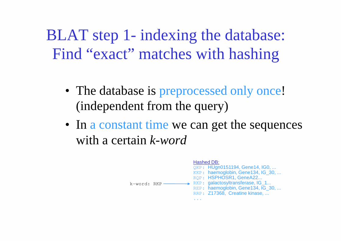
BLAT step 1- indexing the database: Find “exact” matches with hashing

• The database is preprocessed only once! (independent from the query)

• In a constant timewe can get the sequences • In a constant timewe can get the sequences with a certain k-word

k-word: RKP

Hashed DB:QKP: HUgn0151194, Gene14, IG0, ...KKP: haemoglobin, Gene134, IG_30, ...RQP: HSPHOSR1, GeneA22...RKP: galactosyltransferase, IG_1...REP: haemoglobin, Gene134, IG_30, ...RRP: Z17368, Creatine kinase, ......

BLAT – step2: scanning the DB

• Hit criteria

• In a constant time we can get the

• Sequences with a certain k-word

• Relaxing hit definition -> improve • Relaxing hit definition -> improve sensitivity

- allow imperfect hits

- costly, huge hash grows a few times!

shorten k (would lead to FP), but expect two hits (see BLAST two-hit method)

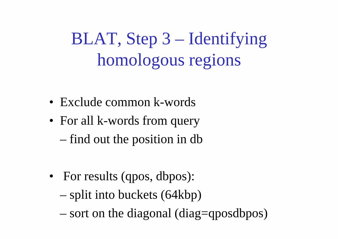
BLAT, Step 3 – Identifying homologous regions

• Exclude common k-words

• For all k-words from query• For all k-words from query

– find out the position in db

• For results (qpos, dbpos):

– split into buckets (64kbp)

– sort on the diagonal (diag=qposdbpos)

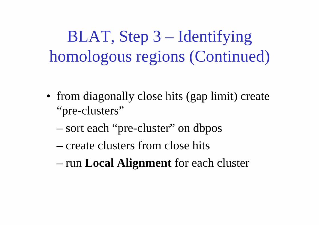
BLAT, Step 3 – Identifying homologous regions (Continued)

• from diagonally close hits (gap limit) create “pre-clusters”“pre-clusters”

– sort each “pre-cluster” on dbpos

– create clusters from close hits

– run Local Alignment for each cluster

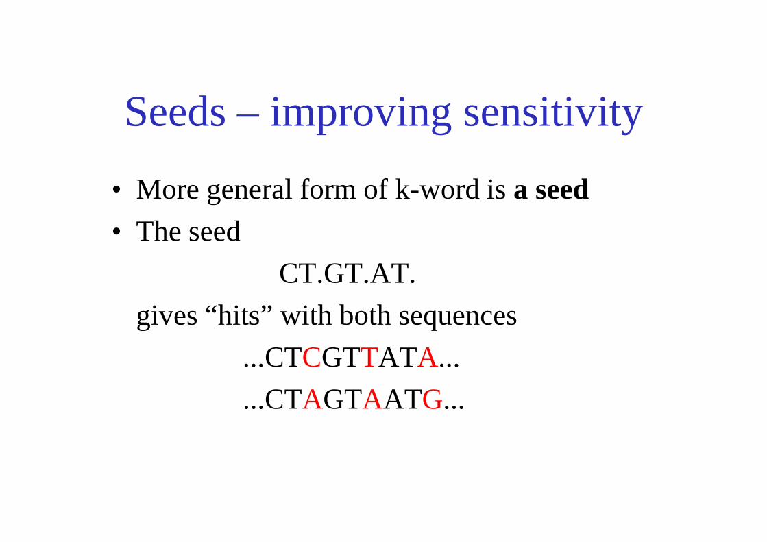
Seeds – improving sensitivity

• More general form of k-word is a seed• The seed

CT.GT.AT.CT.GT.AT.

gives “hits” with both sequences

...CTCGTTATA...

...CTAGTAATG...

HMM-based homology searching

• Most widely used HMM-based profile searchingtools currently are SAM-T2K (Karplus et al.,2000) and HMMER2 (Eddy, 1998)

• Formal probabilistic basis and consistent theory• Formal probabilistic basis and consistent theorybehind gap and insertion scores

• HMMs good for profile searches, not as good foralignment

• HMMs areslow

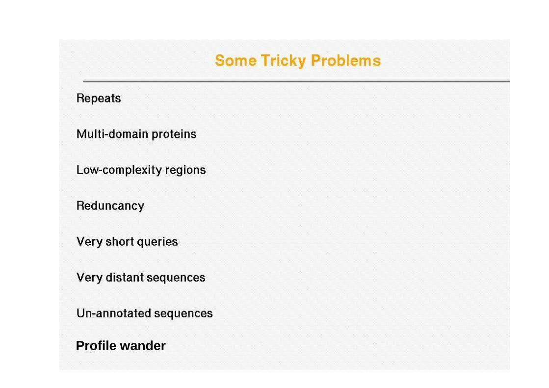
Profile wander

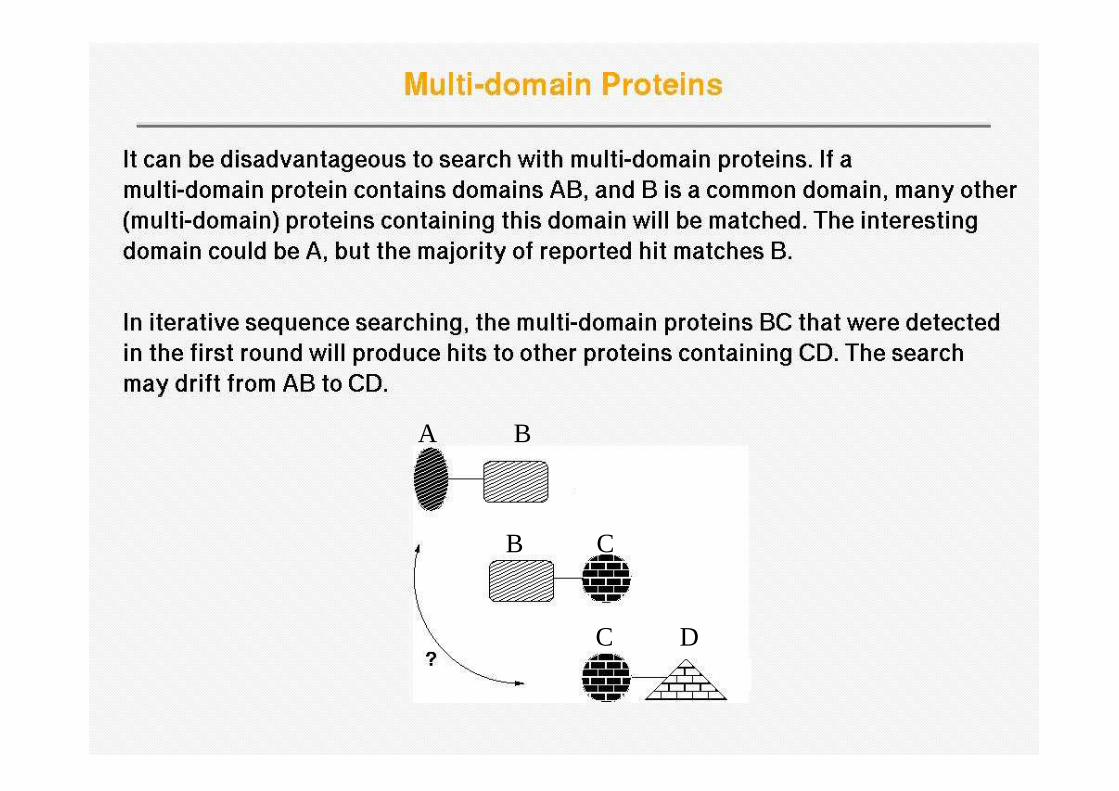
A B

B C

C D

Multi-domain Proteins (cont.)• A common conserved protein domain such as the tyrosine

kinase domain can make weak but relevant matches to other domain types appear very low in the hit list, so that they are missed (e.g. only appearing after 5000 kinase hits)

• Sequences containing low-complexity regions, such as coiled coils and transmembrane regions, can cause an explosion of the search rather than convergence because of the absence of any strong sequence signals. explosion of the search rather than convergence because of the absence of any strong sequence signals.

• Conversely, some searches may lead to premature convergence; this occurs when the PSSM is too strict only allowing matches to very similar proteins, i.e., sequences with the same domain organization as the query are detected but no homologues with different domain combinations. In this case the power of iteration is not used fully.

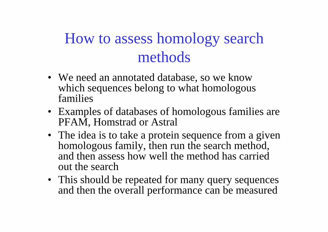
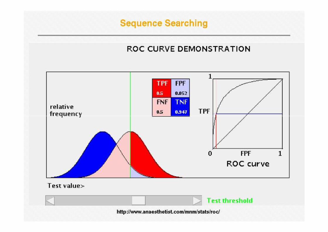
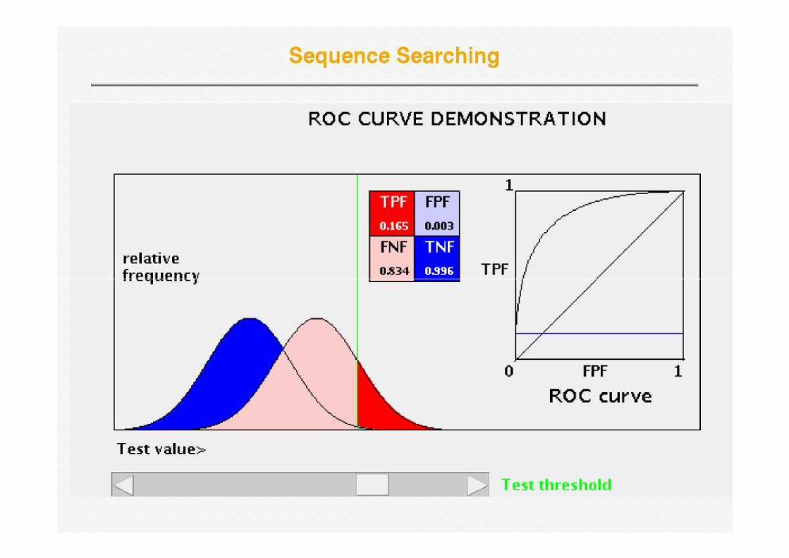
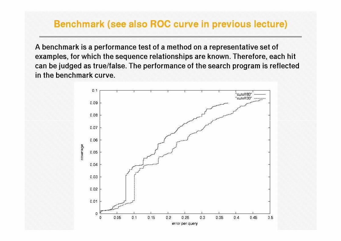
How to assess homology search methods

• We need an annotated database, so we know which sequences belong to what homologous families

• Examples of databases of homologous families are PFAM, Homstrad or Astral

• Examples of databases of homologous families are PFAM, Homstrad or Astral

• The idea is to take a protein sequence from a given homologous family, then run the search method, and then assess how well the method has carried out the search

• This should be repeated for many query sequences and then the overall performance can be measured

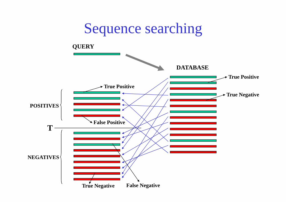
Sequence searchingQUERY

DATABASE

True Positive

True Negative

True Positive

False Positive

True Negative False Negative

T

POSITIVES

NEGATIVES

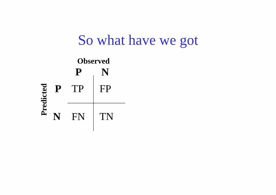
So what have we got

TP FP

Observed

Pre

dict

ed

P

P

N

TNFNPre

dict

ed

N

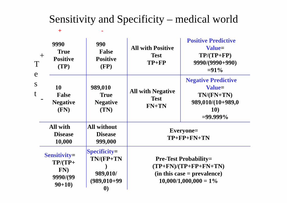
Sensitivity and Specificity – medical world+ -

Test

+

9990True

Positive(TP)

990False

Positive(FP)

All with Positive Test

TP+FP

Positive Predictive Value=

TP/(TP+FP)9990/(9990+990)

=91%

-

10False

Negative

989,010True

Negative

All with Negative Test

Negative Predictive Value=

TN/(FN+TN)989,010/(10+989,0- Negative

(FN) Negative

(TN)

TestFN+TN

989,010/(10+989,010)

=99.999%

All with Disease10,000

All without Disease999,000

Everyone=TP+FP+FN+TN

Sensitivity=TP/(TP+

FN)9990/(9990+10)

Specificity=TN/(FP+TN

)989,010/

(989,010+990)

Pre-Test Probability=(TP+FN)/(TP+FP+FN+TN)(in this case = prevalence)

10,000/1,000,000 = 1%

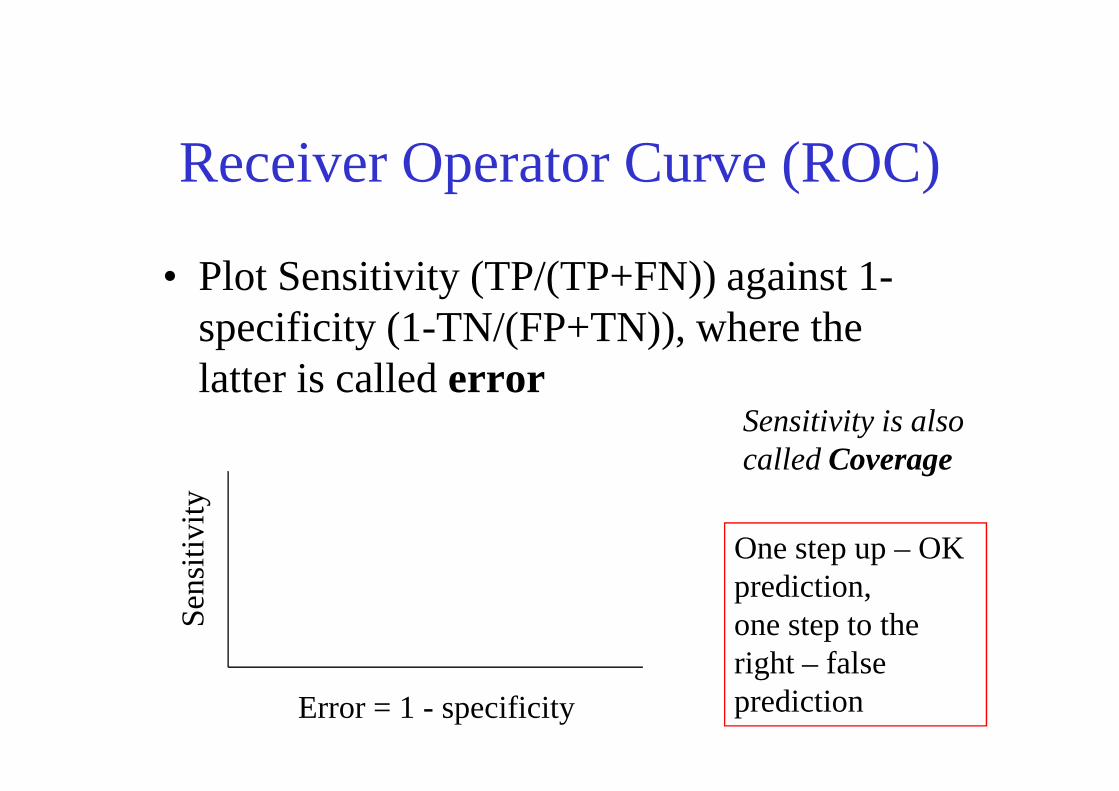
Receiver Operator Curve (ROC)

• Plot Sensitivity (TP/(TP+FN)) against 1-specificity (1-TN/(FP+TN)), where the latter is called errorlatter is called error

Error = 1 - specificity

Sens

itiv

ity

Sensitivity is also called Coverage

One step up – OK prediction, one step to the right – false prediction

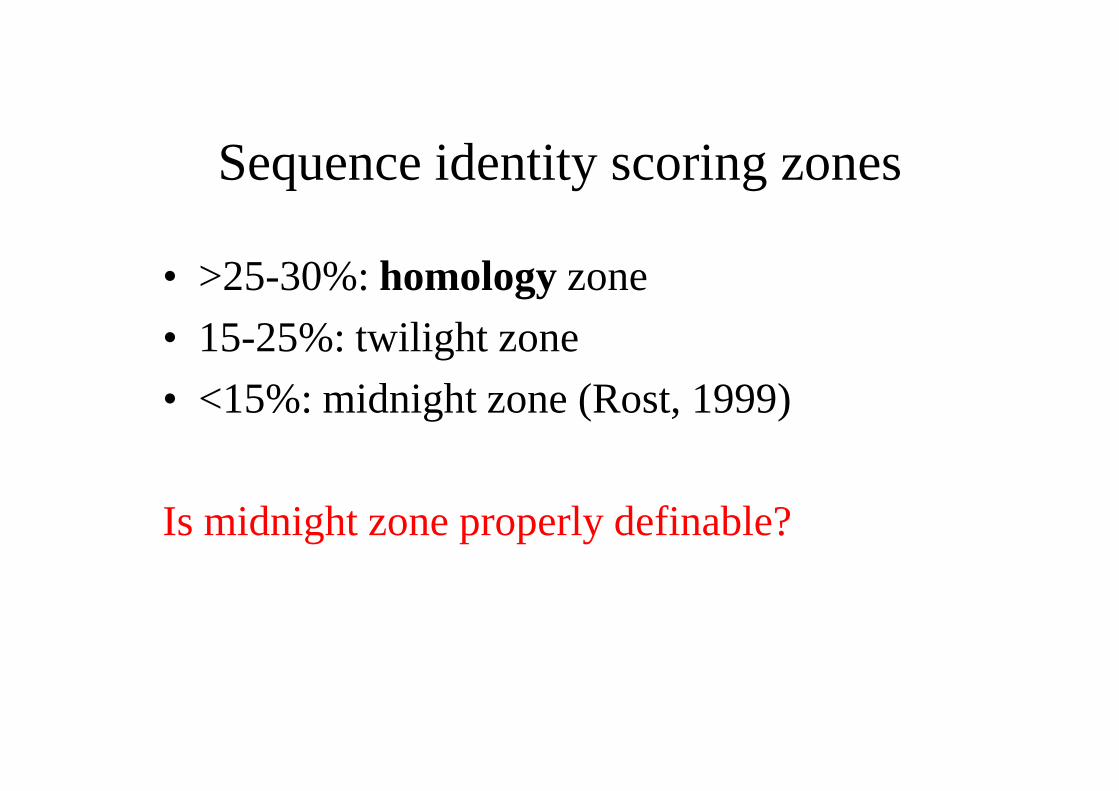
Sequence identity scoring zones

• >25-30%: homology zone

• 15-25%: twilight zone

• <15%: midnight zone (Rost, 1999)• <15%: midnight zone (Rost, 1999)

Is midnight zone properly definable?