Embed Size (px)
Citation preview

G-SURF Mid-Presenta-tion
Presentation Date :
2014.07.29
Presented by : Kyuewang
Lee
in CVL Laboratory, GIST
<< About what I’ve studied about Filters and its implementation >>
( Focused on Tracking & Detection Technology )

Theme #01. Filters in Track-ing• We are talking about filters in “Signal Processing”
• It is a device that removes some components or features from a signal
• We can classify filters in various aspects and these classifying properties are related to the property of the signal
01. Linear X Non-Linear 02. Time-Invariant X Time-Variant 03. Causal X Not-Causal 04. Analog X Digital 05. Discrete-Time X Continuous-Time ETC.
• So why “FILTERS” on (T & D) ???

Theme #01. Filters in Track-ing#01. Linear Filter Terminolo-giesLow-pass Filter• Low-pass Filter• High-pass Filter• Band-pass Filter• Band-stop Filter( Notch Filter )• Comb Filter• All-pass Filter( Only phase is modi-
fied )
Low-pass Filters are important in erasing “White Noises”
White Noise Noises mix to-
gether!!
※ Even if the object is non-linear, we can approximate it into
piecewise linear objectsThink of Taylor’s Approxima-
tion!
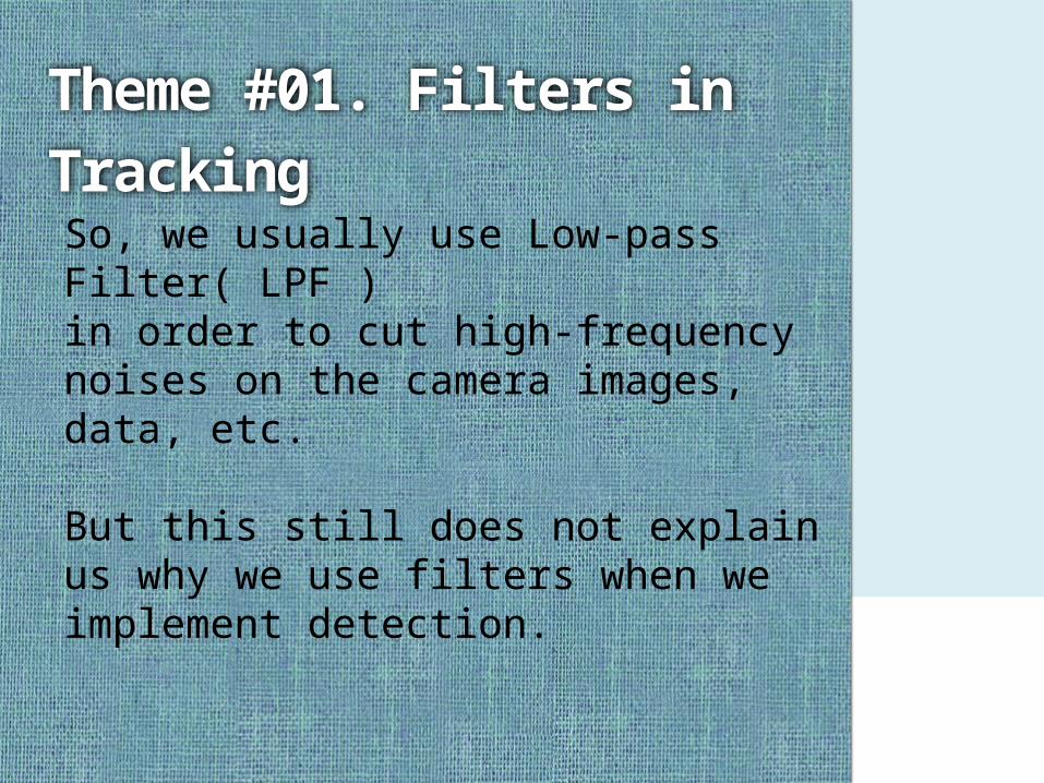
Theme #01. Filters in Track-ingSo, we usually use Low-pass Filter( LPF )in order to cut high-frequency noises on the camera images, data, etc.
But this still does not explain us why we use filters when we implement detection.

Theme #01. Filters in Track-ing• Batch Filter & Recursive Filter
Batch System : Uses Empirical Method
Recursive System : Uses Deductive Method※ I’ll explain this in more detail
Theme #01. Filters in Track-ing
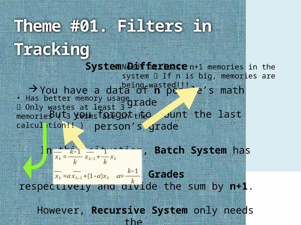
System Difference
You have a data of n people’s math grade But you forgot to count the last person’s
grade
In this situation, Batch System has to Add up All Grades
respectively and divide the sum by n+1.
However, Recursive System only needs the previous average value, last person’s
grade and n to derive present average value.
• Needs at least n+1 memories in the system If n is big, memories are being wasted!!!
• Has better memory usage Only wastes at least 3 memories ( 3 terms are in the calculation!! )
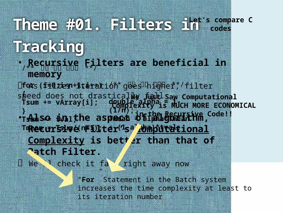
Theme #01. Filters in Track-ing• Recursive Filters are beneficial in
memory As filter iteration goes higher, filter speed does not drastically fall
• Also in the aspect of algorithm, Re-cursive Filter’s Computational Com-plexity is better than that of Batch Filter.
We’ll check it fast right away now
Let’s compare C codes
/** 평균 다시 구하기 **/
for (i=0;i<n+1;i++){Tsum += vArray[i];}Tsum += tval;Tmean = Tsum/(n+1);
/** 평균 다시 구하기 **/
double alpha = 1-(1/n);Tmean = alpha*Tmean + (1-alpha)*tval;
“For” Statement in the Batch system increases the time complexity at least to its iteration number
We Just Saw Computational Complex-ity is MUCH MORE ECONOMICAL in
the Recursive Code!!
Theme #01. Filters in Track-ing
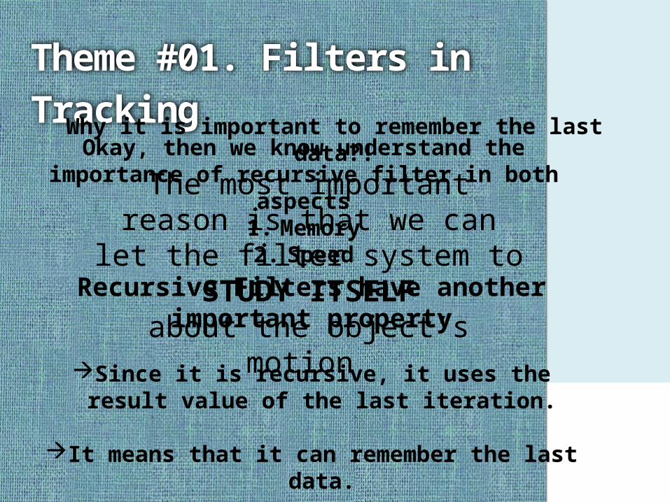
Okay, then we know understand the im-portance of recursive filter in both as-
pects1. Memory2. Speed
Recursive Filters have another im-portant property
Since it is recursive, it uses the result value of the last iteration.
It means that it can remember the last data.
Why it is important to remember the last data?!
The most important reason is that we can let the filter
system to STUDY ITSELF
about the object’s motion

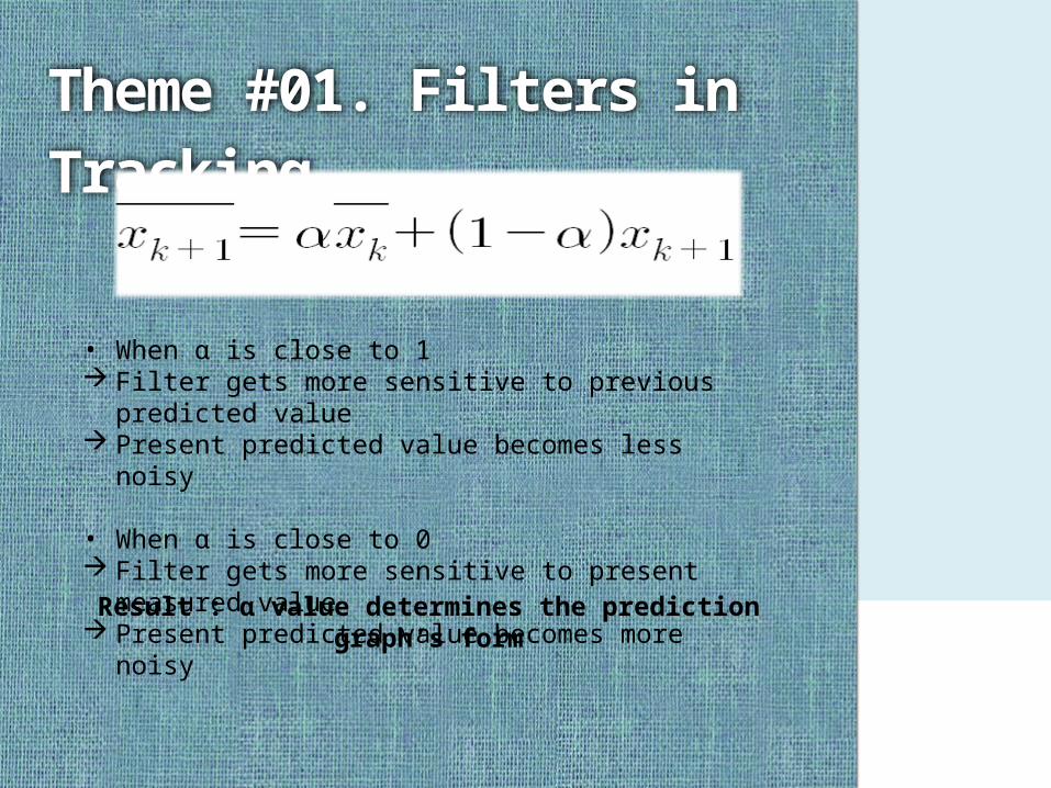
Theme #01. Filters in Track-ing※ One example of LPF Exponentially Weighted Moving Average Fil-terFirstly, this filter became the fundamental notion for the
famous “Kalman Filter”
Also, classified as 1st ordered Low-pass Filter and this is used in various types of studies, especially in Economics.You can recognize that this equation is similar to set-
ting a division point between two points.
This is the reason that we call this “Weighted Filter”We can determine whether to grant more importance to the previous data prediction value or to the present
data measurement value
Theme #01. Filters in Track-ing
• When α is close to 1 Filter gets more sensitive to previous predicted
value Present predicted value becomes less noisy
• When α is close to 0 Filter gets more sensitive to present measured
value Present predicted value becomes more noisyResult : α value determines the prediction
graph’s form
Theme #02. Kalman Filter
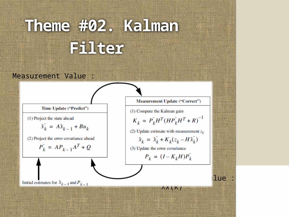
Measurement Value : z(k)
Kalman Fil-ter
Predicted Value : Xx(k)
5 Equations consisting the Kalman Filter
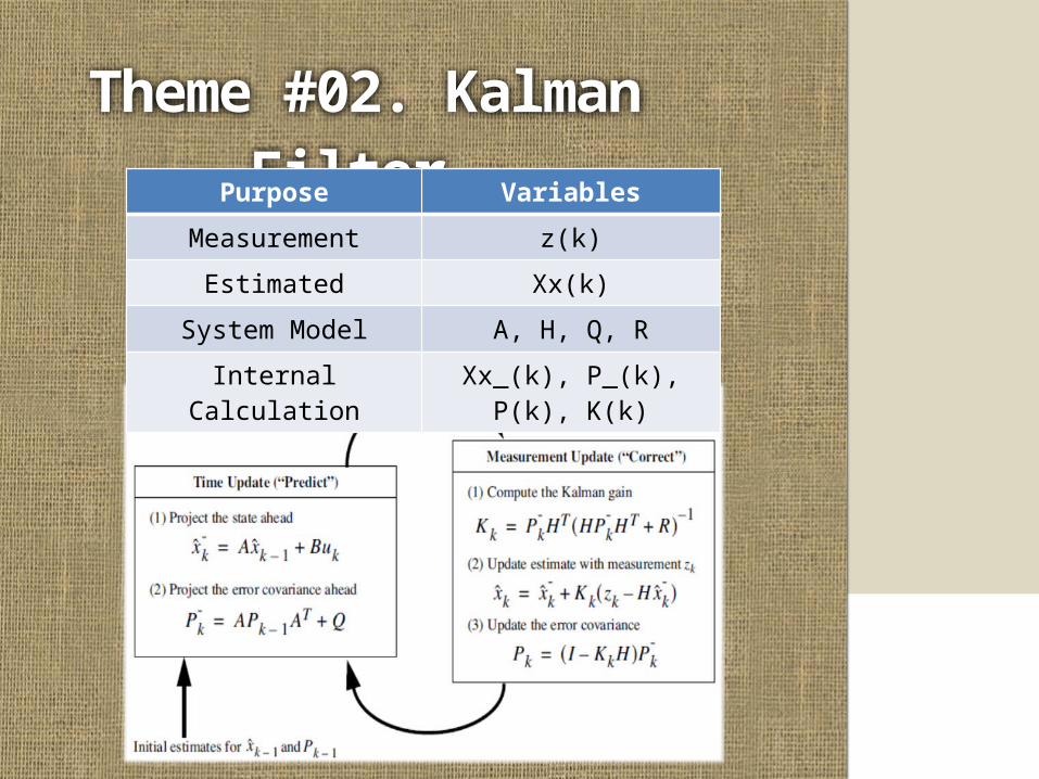
Theme #02. Kalman Filter Purpose Variables
Measurement z(k)
Estimated Xx(k)
System Model A, H, Q, R
Internal Calculation Xx_(k), P_(k), P(k), K(k)

Theme #02. Kalman Filter
<01> Measurement z(k)
• The “NOISY” input signals that the filter feeds in
• Can be approximated into “Ground_Truth + N(0,σ)” ( Signals that have standard deviation of σ from ground truth )
• N(0,σ) is assumed to be the noise of this measurement value.
( e.g. Noise is assumed to follow the normal distribution of mean value 0 )

Theme #02. Kalman Filter
<02> Estimated Value Xx(k)
• The estimated value of one iteration of Kalman Filter
• This value is feed-backed into the filter again
• This is also called “Estimated Status Value”
• On the first iteration, we usually set this value as the orig-inal state of the object unless there is no condition for starting point
Theme #02. Kalman Filter
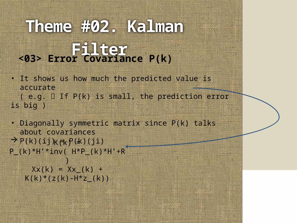
<03> Error Covariance P(k)
• It shows us how much the predicted value is accurate ( e.g. If P(k) is small, the prediction error is big )
• Diagonally symmetric matrix since P(k) talks about co-variances
P(k)(ij) = P(k)(ji)
K(k) = P_(k)*H’*inv( H*P_(k)*H’+R )Xx(k) = Xx_(k) + K(k)*(z(k)-
H*z_(k))

Theme #02. Kalman Filter
<04> System Models
• A : State Transition Model applied to the previous state x(k-1)
This determines the dynamic motion state of the object. Therefore if the object moves in uniformly accelerated motion of straight line, the matrix A would be different from that which moves in uniform circular motion.
• H : Observation Model which maps the true state space x(k) into the observed space z(k)
• Q : Covariance Matrix for the process noise( State Variable Noise ) w(k) ~ N( 0, Q(k) )
• R : Covariance Matrix for the zero mean Gaussian white noise( Measurement Noise ) v(k) ~ N( 0, R(k) )
• B : Control-Input Model which considers external fac-tors
System Modelingx(k) = A*x(k-1) + B*u(k) +
w(k)z(k) = H*x(k) + v(k)
u(k) is the Control Vector
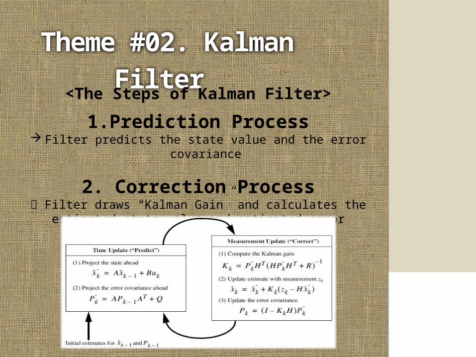
Theme #02. Kalman Filter
<The Steps of Kalman Filter>
1.Prediction Process Filter predicts the state value and the error covariance
2. Correction Process Filter draws “Kalman Gain” and calculates the estimated
state value and estimated error covariance

Theme #02. Kalman Filter
Correction Process
• K(k) = P_(k)*H’*inv( H*P_(k)*H’+R ) Kalman Gain K(k)
• Xx(k) = Xx_(k) + K(k)*( z(k)-H*x_(k) ) Estimation Xx(k)
• P(k) = P_(k) – K(k)*H*P_(k) Error Covariance P(k)
What if H is I ( Identity Matrix ) ??
The equation becomes like below form
Xx(k) = ( I-K(k)*H )*Xx_(k) + K(k)*z(k) Xx(k) = ( I-K(k) )*Xx_(k) + K(k)*z(k)
These two equation are in same form
Thus the method of solving estimation value is in actual, solving this exponentially weighted equa-
tion
K(k) = P_(k)*H’*inv( H*P_(k)*H’+R ) Kalman Gain
The weight factor( Kalman Gain ) differs every itera-tion
This filter can balance the importance by it-self!!

Theme #02. Kalman Filter
Prediction Process
• Xx_(k) = A*Xx(k-1) + B*u(k)
• P_(k) = A*P(k-1)*A’ + QLinear Modeling
This process makes the prediction values for each variablesand these are to be used in the correction process to yield es-timation values. This is the singular iteration and we do it ‘k’ times.

Theme #02. Kalman Filter
Actual Implementation
• 01. Sine function tracking
Implemented with MATLAB
Ground Truth Estimated // Ground Truth
Measured // Estimated A = // Q =
H = // R = 50*
P = 25* // System ModelsStandard Deviation ( σ ): 0.1
A = Uniform Acceleration Linear Model
Estimated // Ground Truth
Nonlinear
Linear

감사합니다


![[Cvl]-Bahan Kontruksi Teknik](https://img.pdfslide.net/doc/110x75/55cf8678550346484b97f5af/cvl-bahan-kontruksi-teknik.jpg)


![[Cvl] Statistika Probabilitas](https://img.pdfslide.net/doc/110x75/55cf91a1550346f57b8f1c4c/cvl-statistika-probabilitas.jpg)


![[Cvl] Pengantar Statistika](https://img.pdfslide.net/doc/110x75/55cf917e550346f57b8dea42/cvl-pengantar-statistika.jpg)


![[Cvl]-Pengantar Manajemen Proyek](https://img.pdfslide.net/doc/110x75/563dba6e550346aa9aa58e89/cvl-pengantar-manajemen-proyek.jpg)
![[cvl]-Pemindahan Tanah Mekanis.pdf](https://img.pdfslide.net/doc/110x75/55cf8c625503462b138be4fd/cvl-pemindahan-tanah-mekanispdf.jpg)


![[Cvl] Aplikasi Excel](https://img.pdfslide.net/doc/110x75/577cdd461a28ab9e78acaa94/cvl-aplikasi-excel.jpg)
