G x E interaction and Phenotypic stability General Considerations in potato breeding

S K Luthra Principal Scientist

• Genetics: Study of heredity and variation.

• Breeding: Consist of principles and methods required for favourable changing the genetic constitution of crop. Plant breeding aims to develop an improved crop variety utilized by farmers for commercial cultivation.

• Variety: A taxonomic subdivision of a species consisting of naturally occurring or selectively bred populations or individuals that differ from the remainder of the species in certain minor characteristics.

• Cultivar: A plant or grouping of plants selected for desirable characteristics that can be maintained by propagation.

• Clone: Clone group of identical plants derived from single plants through asexual propagation.

• Single outstanding plant selected from population form the basis of variety.

Potato breeding

• No authentic records to show, when potatoes were subjected to selection.

• Probably potato selection started as soon as potato cultivation started.

• Growers started to exercise choice among the different type available to them.

• Potato breeding in the modern sense began in 1807 in England when Knight (1807) made deliberate hybridization between different varieties by artificial pollination.

• Acceleration of potato breeding was a direct result of the severe late blight epidemic, which swept Europe in the years 1843 to 1847.

• Potato breeding gained impetus with the increase in understanding of the science of heredity and rediscovery of Mendel’s law of inheritance in 1900.

• An ideal potato variety affects not only yield and quality but also production cost, environmental issues (requirement of pesticides), post harvest losses (susceptibility to mechanical damage or sprouting) and yield of future crops (Struik and Wiersema, 1999).

• More than 50 traits should be combined in a modern potato variety (Ross, 1986).

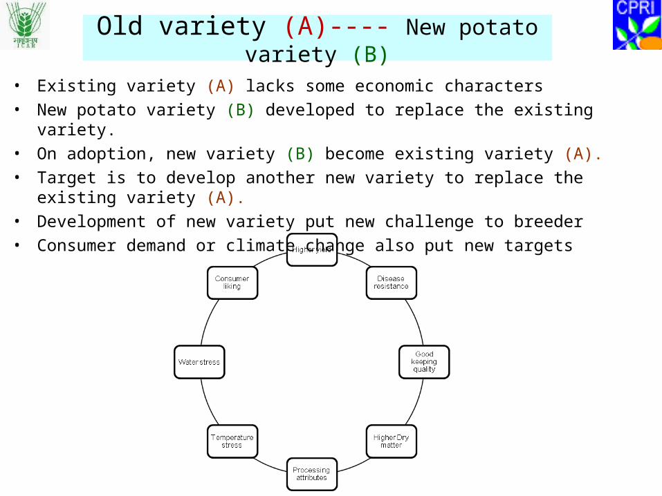
Old variety (A)---- New potato variety (B)

• Existing variety (A) lacks some economic characters

• New potato variety (B) developed to replace the existing variety.

• On adoption, new variety (B) become existing variety (A).

• Target is to develop another new variety to replace the existing variety (A).

• Development of new variety put new challenge to breeder

• Consumer demand or climate change also put new targets

•Germplasm collection, evaluation and selection of parents

•Exploitation of genetic resources for creation of genetic variability

•Evaluation of segregating population and selection.

•Introduction in AICRP for multi-location evaluation

Potato Breeding

Features of adaptations

1.It is the process of adjustment of living organism to the changing environment.

2.It favours those characters which are advantageous for survival and

through which an individual acquires adaptive or fitness to the given

environment.

3.In the process of adaptation survival is the main concern.

4.Natural selection play an important role in the process of adaptation

Adaptation

Adaptation refers to changes in structure or function of an individual or population which lead to better survival or greater fitness in the given environment.

Features of adaptability

1.Adaptable genotypes produce narrow range of phenotypes in different environments.

2.Adaptability leads to stable performance of a genotype over a wide range of environments.

3.General genotypic and general population adaptations are the examples of wide adaptability.

4.Varietal adaptability of is the result of genetic and physiological homeostasis.

5.Productivity is the main concern in varietal adaptability.

AdaptabilityAdaptability is the capacity of a genotype or population for genetic changes in adaptation

Genetic homeostasis is the ability of genotype to withstands environmental fluctuations (Lerner, 1954). Thus variability in the performance over a wide range of environments can be used a criterion for measure of phenotypic stability.

Physiological homeostasis refers to physiological or developmental capacity of a genotype to the environment fluctuations. The internal self regulatory mechanisms enable the individual to adjust to the fluctuating environment by resisting such changes. It is generally higher in heterozygous genotypes than in homozygous one

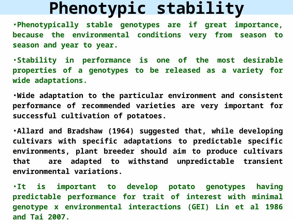
Phenotypic stability•Phenotypically stable genotypes are if great importance, because the environmental conditions very from season to season and year to year.

•Stability in performance is one of the most desirable properties of a genotypes to be released as a variety for wide adaptations.

•Wide adaptation to the particular environment and consistent performance of recommended varieties are very important for successful cultivation of potatoes.

•Allard and Bradshaw (1964) suggested that, while developing cultivars with specific adaptations to predictable specific environments, plant breeder should aim to produce cultivars that are adapted to withstand unpredictable transient environmental variations.

•It is important to develop potato genotypes having predictable performance for trait of interest with minimal genotype x environmental interactions (GEI) Lin et al 1986 and Tai 2007.

•GEI are extremely important in the development and evaluation of plant varieties because they reduce the genotypic stability values under diverse environments (Habert et al 1995).

G X E Interaction

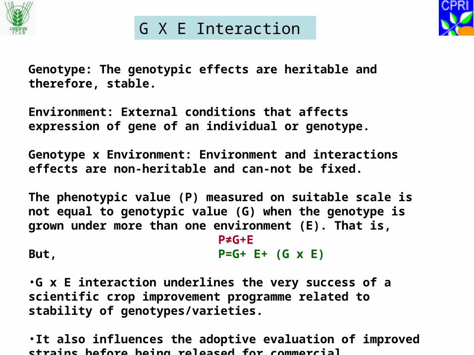
Genotype: The genotypic effects are heritable and therefore, stable. Environment: External conditions that affects expression of gene of an individual or genotype.

Genotype x Environment: Environment and interactions effects are non-heritable and can-not be fixed.

The phenotypic value (P) measured on suitable scale is not equal to genotypic value (G) when the genotype is grown under more than one environment (E). That is,

P≠G+EBut, P=G+ E+ (G x E)

•G x E interaction underlines the very success of a scientific crop improvement programme related to stability of genotypes/varieties.

•It also influences the adoptive evaluation of improved strains before being released for commercial cultivation.

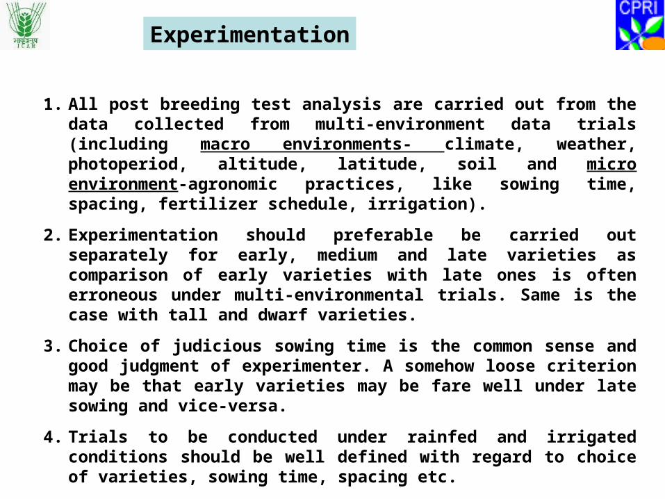
1. All post breeding test analysis are carried out from the data collected from multi-environment data trials (including macro environments- climate, weather, photoperiod, altitude, latitude, soil and micro environment-agronomic practices, like sowing time, spacing, fertilizer schedule, irrigation).

2. Experimentation should preferable be carried out separately for early, medium and late varieties as comparison of early varieties with late ones is often erroneous under multi-environmental trials. Same is the case with tall and dwarf varieties.

3. Choice of judicious sowing time is the common sense and good judgment of experimenter. A somehow loose criterion may be that early varieties may be fare well under late sowing and vice-versa.

4. Trials to be conducted under rainfed and irrigated conditions should be well defined with regard to choice of varieties, sowing time, spacing etc.

Experimentation

Stability Analysis

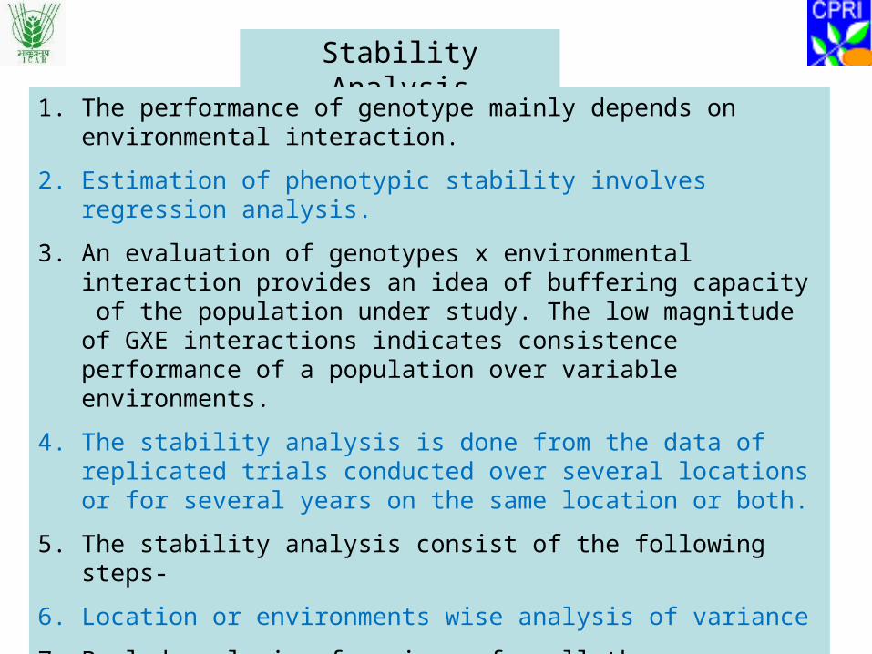
1. The performance of genotype mainly depends on environmental interaction.

2. Estimation of phenotypic stability involves regression analysis.

3. An evaluation of genotypes x environmental interaction provides an idea of buffering capacity of the population under study. The low magnitude of GXE interactions indicates consistence performance of a population over variable environments.

4. The stability analysis is done from the data of replicated trials conducted over several locations or for several years on the same location or both.

5. The stability analysis consist of the following steps-

6. Location or environments wise analysis of variance

7. Pooled analysis of variance for all the location/environments.

8. If GXE interactions are found significant, the stability analysis can be done using the appropriate model-

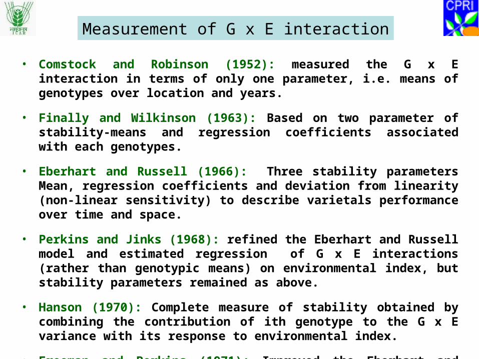
• Comstock and Robinson (1952): measured the G x E interaction in terms of only one parameter, i.e. means of genotypes over location and years.

• Finally and Wilkinson (1963): Based on two parameter of stability-means and regression coefficients associated with each genotypes.

• Eberhart and Russell (1966): Three stability parameters Mean, regression coefficients and deviation from linearity (non-linear sensitivity) to describe varietals performance over time and space.

• Perkins and Jinks (1968): refined the Eberhart and Russell model and estimated regression of G x E interactions (rather than genotypic means) on environmental index, but stability parameters remained as above.

• Hanson (1970): Complete measure of stability obtained by combining the contribution of ith genotype to the G x E variance with its response to environmental index.

• Freeman and Perkins (1971); Improved the Eberhart and Russell model with respect to making environmental index really independent variable.

Measurement of G x E interaction

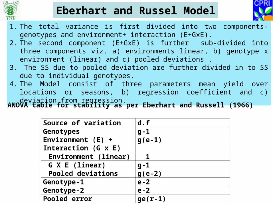
Eberhart and Russel Model1. The total variance is first divided into two components- genotypes and

environment+ interaction (E+GxE).2. The second component (E+GxE) is further sub-divided into three components viz.

a) environments linear, b) genotype x environment (linear) and c) pooled deviations .

3. The SS due to pooled deviation are further divided in to SS due to individual genotypes.

4. The Model consist of three parameters mean yield over locations or seasons, b) regression coefficient and c) deviation from regression.

ANOVA table for stability as per Eberhart and Russell (1966)

Source of variation d.fGenotypes g-1Environment (E) + Interaction (G x E)

g(e-1)

Environment (linear) 1G X E (linear) g-1Pooled deviations g(e-2)

Genotype-1 e-2Genotype-2 e-2Pooled error ge(r-1)

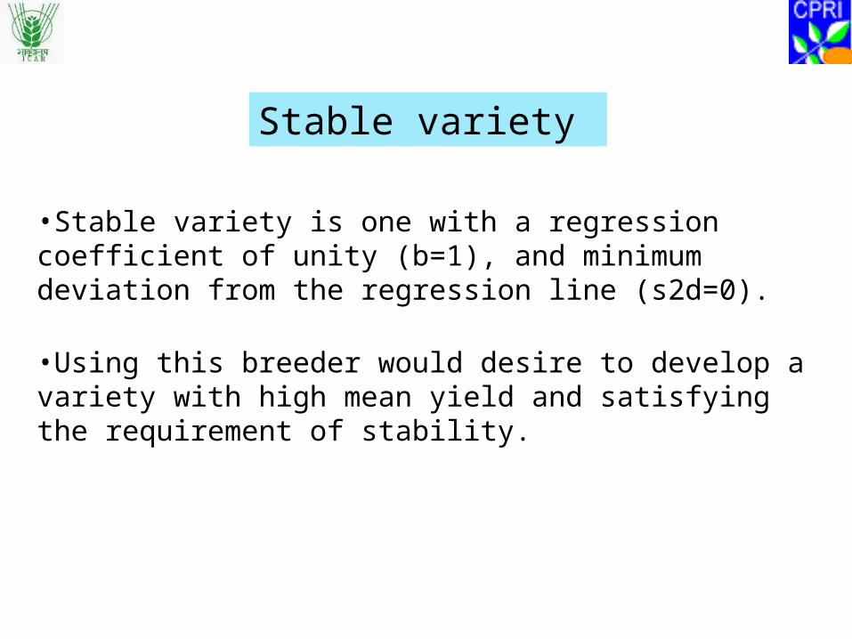
•Stable variety is one with a regression coefficient of unity (b=1), and minimum deviation from the regression line (s2d=0).

•Using this breeder would desire to develop a variety with high mean yield and satisfying the requirement of stability.

Stable variety

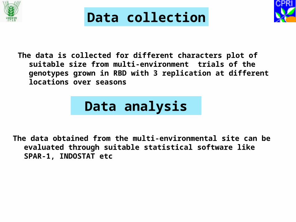
The data is collected for different characters plot of suitable size from multi-environment trials of the genotypes grown in RBD with 3 replication at different locations over seasons

Data collection

The data obtained from the multi-environmental site can be evaluated through suitable statistical software like SPAR-1, INDOSTAT etc

Data analysis

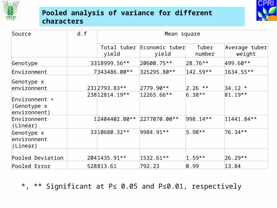
Pooled analysis of variance for different characters

Source d.f Mean square Total tuber yield Economic tuber

yieldTuber number Average tuber

weight

Genotype 3318999.56** 20600.75** 28.76** 499.60**

Environment 7343486.00** 325295.80** 142.59** 1634.55**

Genotype x environnent 2312793.83** 2779.90** 2.26 ** 34.12 *

Environnent + (Genotype x environnent)

23812814.19** 12265.66** 6.38** 81.19**

Environnent (Linear)12404402.00** 2277070.00** 998.14** 11441.84**

Genotype x environnent (Linear)

3310680.32** 9984.91** 5.98** 76.34**

Pooled Deviation 2041435.91** 1532.61** 1.59** 26.29**

Pooled Error 528813.61 792.23 0.99 13.84

*, ** Significant at P≤ 0.05 and P≤0.01, respectively

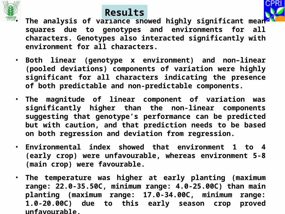
• The analysis of variance showed highly significant mean squares due to genotypes and environments for all characters. Genotypes also interacted significantly with environment for all characters.

• Both linear (genotype x environment) and non–linear (pooled deviations) components of variation were highly significant for all characters indicating the presence of both predictable and non-predictable components.

• The magnitude of linear component of variation was significantly higher than the non-linear components suggesting that genotype’s performance can be predicted but with caution, and that prediction needs to be based on both regression and deviation from regression.

• Environmental index showed that environment 1 to 4 (early crop) were unfavourable, whereas environment 5-8 (main crop) were favourable.

• The temperature was higher at early planting (maximum range: 22.0-35.50C, minimum range: 4.0-25.00C) than main planting (maximum range: 17.0-34.00C, minimum range: 1.0-20.00C) due to this early season crop proved unfavourable.

Results

• A variety with unit regression coefficient (bi=1) and deviation from

regression not significantly different from zero (S2di=0) is said to be

stable.

• Accessions with bi values significantly higher than 1 and non-significant

deviation from regression are expected to perform better in the

favourable environments.

• Accessions with bi values significantly lower than 1 and non-significant

deviations from the regression are more suitable for low yielding

environments.

• Those which have both bi and deviation from regression significant are

unstable.

• Stable genotypes had not necessarily significantly high mean values for

different characters.

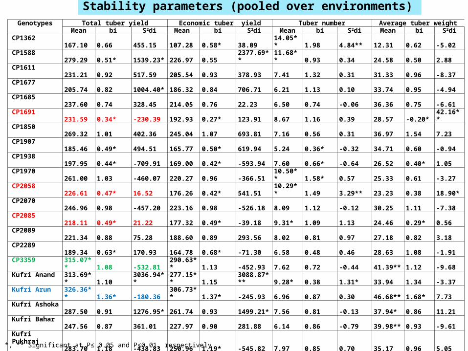
Stability parameters (pooled over environments)Genotypes Total tuber yield Economic tuber yield Tuber number Average tuber weight

Mean bi S2di Mean bi S2di Mean bi S2di Mean bi S2diCP1362 167.10 0.66 455.15 107.28 0.58* 38.09 14.05** 1.98 4.84** 12.31 0.62 -5.02CP1588 279.29 0.51* 1539.23* 226.97 0.55 2377.69** 11.68** 0.93 0.34 24.58 0.50 2.88CP1611 231.21 0.92 517.59 205.54 0.93 378.93 7.41 1.32 0.31 31.33 0.96 -8.37CP1677 205.74 0.82 1004.40* 186.32 0.84 706.71 6.21 1.13 0.10 33.74 0.95 -4.94CP1685 237.60 0.74 328.45 214.05 0.76 22.23 6.50 0.74 -0.06 36.36 0.75 -6.61CP1691 231.59 0.34* -230.39 192.93 0.27* 123.91 8.67 1.16 0.39 28.57 -0.20* 42.16**CP1850 269.32 1.01 402.36 245.04 1.07 693.81 7.16 0.56 0.31 36.97 1.54 7.23CP1907 185.46 0.49* 494.51 165.77 0.50* 619.94 5.24 0.36* -0.32 34.71 0.60 -0.94CP1938 197.95 0.44* -709.91 169.00 0.42* -593.94 7.60 0.66* -0.64 26.52 0.40* 1.05CP1970 261.00 1.03 -460.07 220.27 0.96 -366.51 10.50** 1.58* 0.57 25.33 0.61 -3.27CP2058 226.61 0.47* 16.52 176.26 0.42* 541.51 10.29** 1.49 3.29** 23.23 0.38 18.90*CP2070 246.96 0.98 -457.20 223.16 0.98 -526.18 8.09 1.12 -0.12 30.25 1.11 -7.38CP2085 218.11 0.49* 21.22 177.32 0.49* -39.18 9.31* 1.09 1.13 24.46 0.29* 0.56CP2089 221.34 0.88 75.28 188.60 0.89 293.56 8.02 0.81 0.97 27.18 0.82 3.18CP2289 189.34 0.63* 170.93 164.78 0.68* -71.30 6.58 0.48 0.46 28.63 1.08 -1.91CP3359 315.07** 1.08 -532.81 290.63** 1.13 -452.93 7.62 0.72 -0.44 41.39** 1.12 -9.68Kufri Anand 313.69** 1.10 3036.94** 277.15** 1.15 3088.87*** 9.28* 0.38 1.31* 33.94 1.34 -3.37Kufri Arun 326.36** 1.36* -180.36 306.73** 1.37* -245.93 6.96 0.87 0.30 46.68** 1.68* 7.73Kufri Ashoka 287.50 0.91 1276.95* 261.74 0.93 1499.21* 7.56 0.81 -0.13 37.94* 0.86 11.21Kufri Bahar 247.56 0.87 361.01 227.97 0.90 281.88 6.14 0.86 -0.79 39.98** 0.93 -9.61Kufri Pukhraj 283.70 1.18 -438.83 250.96 1.19* -545.82 7.97 0.85 0.70 35.17 0.96 5.05Kufri Pushkar 294.26 0.74 0.56 259.97 0.78 45.15 9.00 0.67 0.11 32.57 0.80 -1.56Kufri Surya 261.33 0.62* -63.07 243.20 0.64* 262.25 6.52 0.58* -0.57 40.71** 1.28 30.11**Kufri Sutlej 326.71** 1.50* 539.41 296.45** 1.49* 822.54 8.30 1.15 0.12 38.46* 1.35 15.39MS/92-1090 310.72** 1.47 2187.97** 292.05** 1.50 2398.80** 6.28 0.74 -0.18 47.45** 1.87* 26.04**MS/93-1344 301.75* 1.37 923.03 276.06* 1.45 2492.65** 7.04 0.38 2.21** 45.22** 2.22 158.50**MS/94-899 308.36** 1.19 356.15 288.87** 1.20 569.09 6.47 0.68* -0.89 46.25** 1.28 30.16*MS/94-1118 312.20** 1.42 1671.22** 289.51** 1.38 1932.88** 7.02 1.13 0.49 43.54** 1.16 2.24MS/95-117 287.19 1.58* 717.40 257.72 1.54* 1489.25* 7.44 1.09 0.71 35.84 1.22 70.06**MS/95-1309 356.71** 1.30 1254.52* 314.52** 1.24 1559.68** 10.57** 1.85* -0.15 34.88 0.70 48.75**MS/97-621 328.31** 1.83* 372.10 283.06** 1.77* 922.10 10.71** 2.19* 1.78* 29.30 1.15 1.22MS/97-1606 302.35* 1.16 1099.95* 278.74** 1.19 1260.33* 6.97 0.85 -0.44 42.41** 1.48 1.11MS/98-6955 310.67** 1.30 624.84 278.78** 1.31 689.83 8.88 1.28* -0.67 34.40 1.27 -0.58MS/98-7208 306.57** 1.60* 2462.47** 262.34 1.50* 1388.31* 10.57** 1.50 3.90** 27.49 0.92 -5.63Mean 269.11 1.00 238.23 1.00 8.19 1.00 34.05 1.00SE 14.30 0.10 14.80 0.20 0.48 0.23 1.94 0.28*, ** Significant at P≤ 0.05 and P≤0.01, respectively

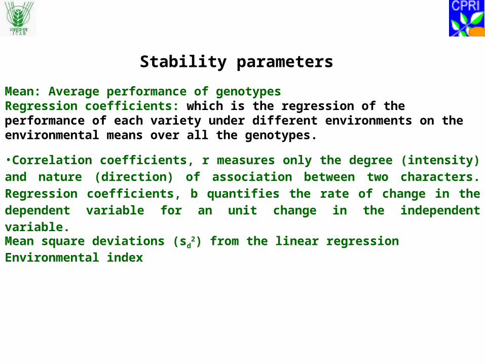
Stability parameters

Mean: Average performance of genotypesRegression coefficients: which is the regression of the performance of each variety under different environments on the environmental means over all the genotypes.

•Correlation coefficients, r measures only the degree (intensity) and nature (direction) of association between two characters. Regression coefficients, b quantifies the rate of change in the dependent variable for an unit change in the independent variable.

Mean square deviations (sd2) from the linear regression

Environmental index