G5BAIM Artificial Intelligence Methods Graham Kendall Ant Algorithms

G5BAIMArtificial Intelligence Methods

Graham KendallAnt Algorithms

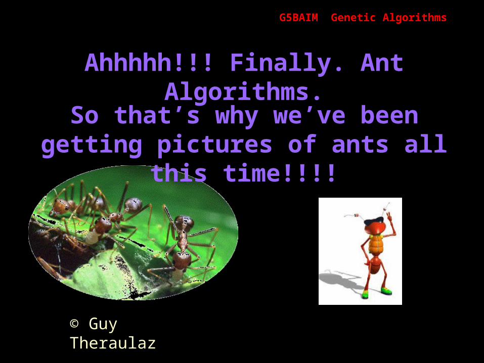
Ahhhhh!!! Finally. Ant Algorithms.

G5BAIM Genetic AlgorithmsG5BAIM Genetic Algorithms

© Guy Theraulaz

So that’s why we’ve been getting pictures of ants all this time!!!!

G5BAIM Ant AlgorithmsG5BAIM Ant Algorithms

Ant Algorithms

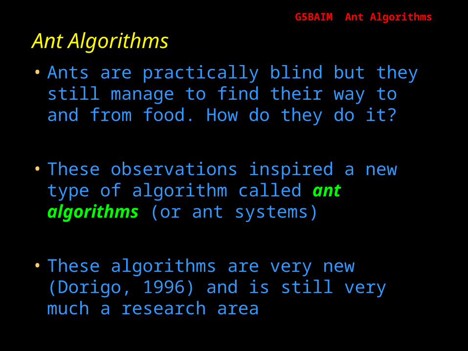
• Ants are practically blind but they still manage to find their way to and from food. How do they do it?

• These observations inspired a new type of algorithm called ant algorithms (or ant systems)

• These algorithms are very new (Dorigo, 1996) and is still very much a research area


Ant Algorithms

• Ant systems are a population based approach. In this respect it is similar to genetic algorithms

• There is a population of ants, with each ant finding a solution and then communicating with the other ants


Ant Algorithms

A

B

C

H

D

F

E

G


Ant Algorithms

A

B

C

D

F

E

d=0.5

d=0.5

d=1

d=1

d=1

d=1


Ant Algorithms

Time, t, is discrete

At each time unit an ant moves a distance, d, of 1

Once an ant has moved it lays down 1 unit of pheromone

At t=0, there is no pheromone on any edge


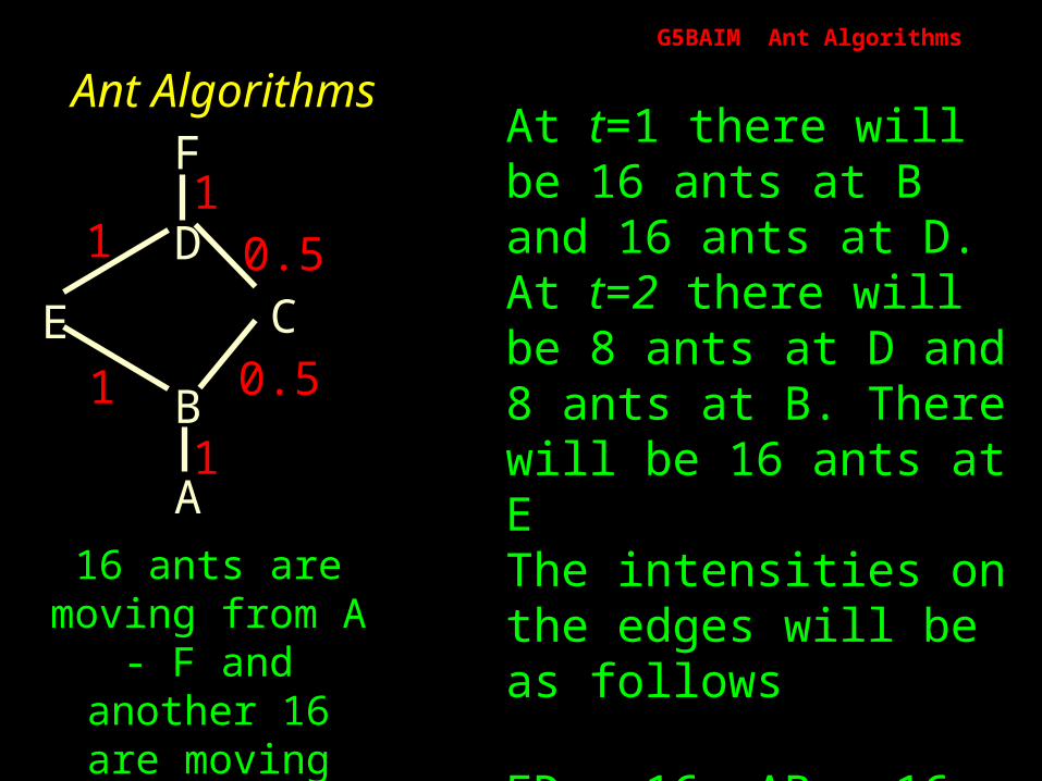
Ant AlgorithmsAt t=1 there will be 16 ants at B and 16 ants at D.At t=2 there will be 8 ants at D and 8 ants at B. There will be 16 ants at EThe intensities on the edges will be as follows

FD = 16, AB = 16, BE = 8, ED = 8, BC = 16 and CD = 16

A

B

C

D

F

E

0.5

0.5

1

1

11

16 ants are moving from A - F and another 16 are

moving from F - A


Ant Algorithms

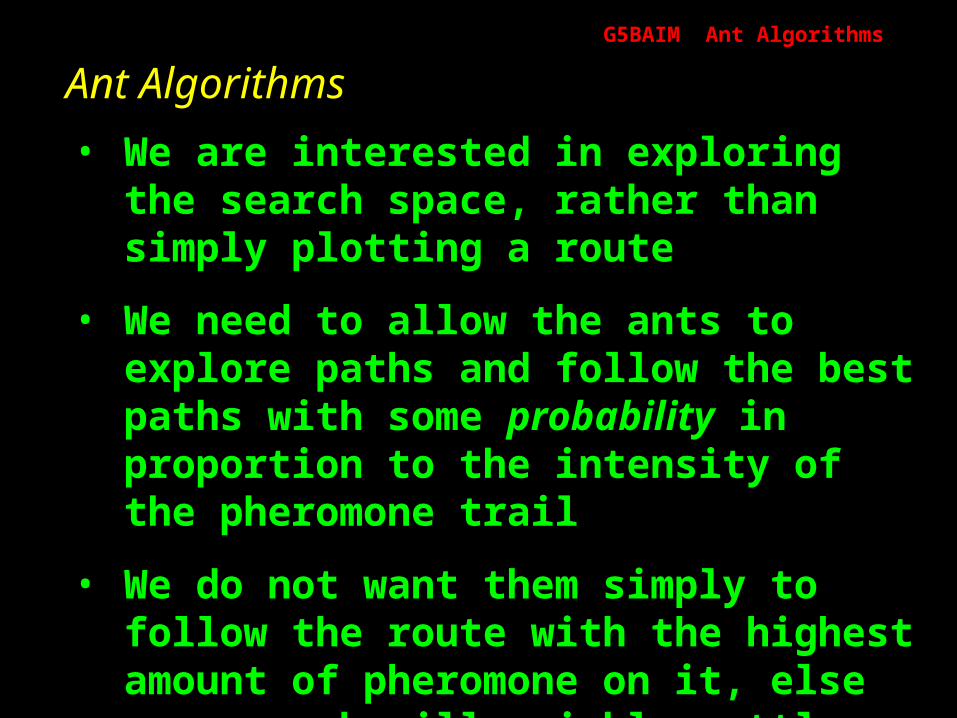
• We are interested in exploring the search space, rather than simply plotting a route

• We need to allow the ants to explore paths and follow the best paths with some probability in proportion to the intensity of the pheromone trail

• We do not want them simply to follow the route with the highest amount of pheromone on it, else our search will quickly settle on a sub-optimal (and probably very sub-optimal) solution


Ant Algorithms

• The probability of an ant following a certain route is a function, not only of the pheromone intensity but also a function of what the ant can see (visibility)

• The pheromone trail must not build unbounded. Therefore, we need “evaporation”


Ant Algorithms and the TSP

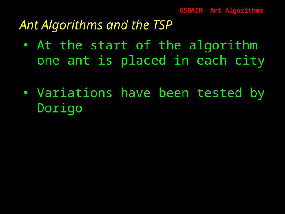
• At the start of the algorithm one ant is placed in each city

• Variations have been tested by Dorigo



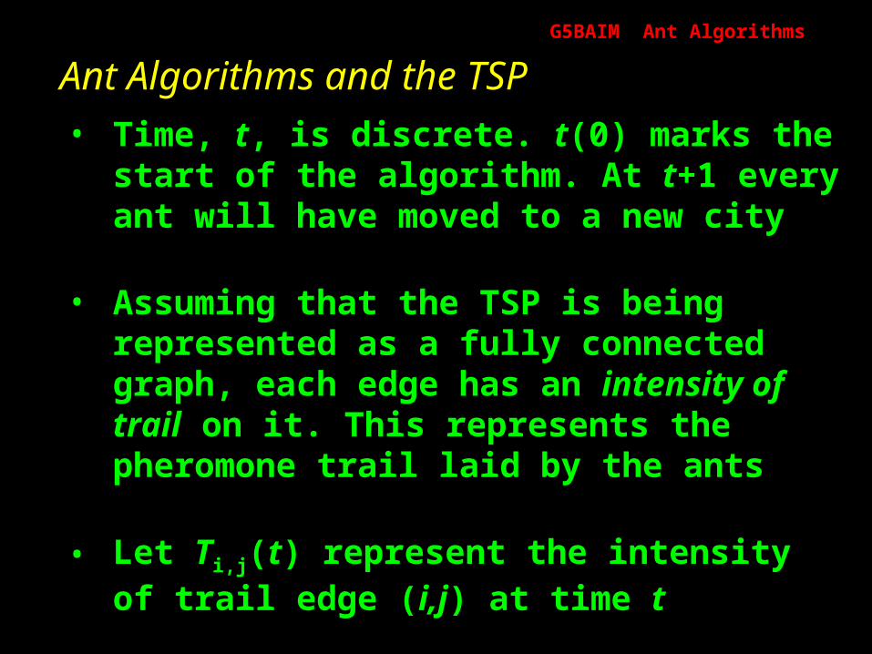
• Time, t, is discrete. t(0) marks the start of the algorithm. At t+1 every ant will have moved to a new city

• Assuming that the TSP is being represented as a fully connected graph, each edge has an intensity of trail on it. This represents the pheromone trail laid by the ants

• Let Ti,j(t) represent the intensity of trail edge (i,j) at time t



• When an ant decides which town to move to next, it does so with a probability that is based on the distance to that city and the amount of trail intensity on the connecting edge

• The distance to the next town, is known as the visibility, nij, and is defined as 1/dij, where, d, is the distance between cities i and j.



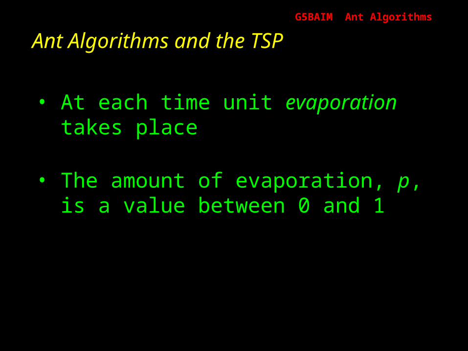
• At each time unit evaporation takes place

• The amount of evaporation, p, is a value between 0 and 1



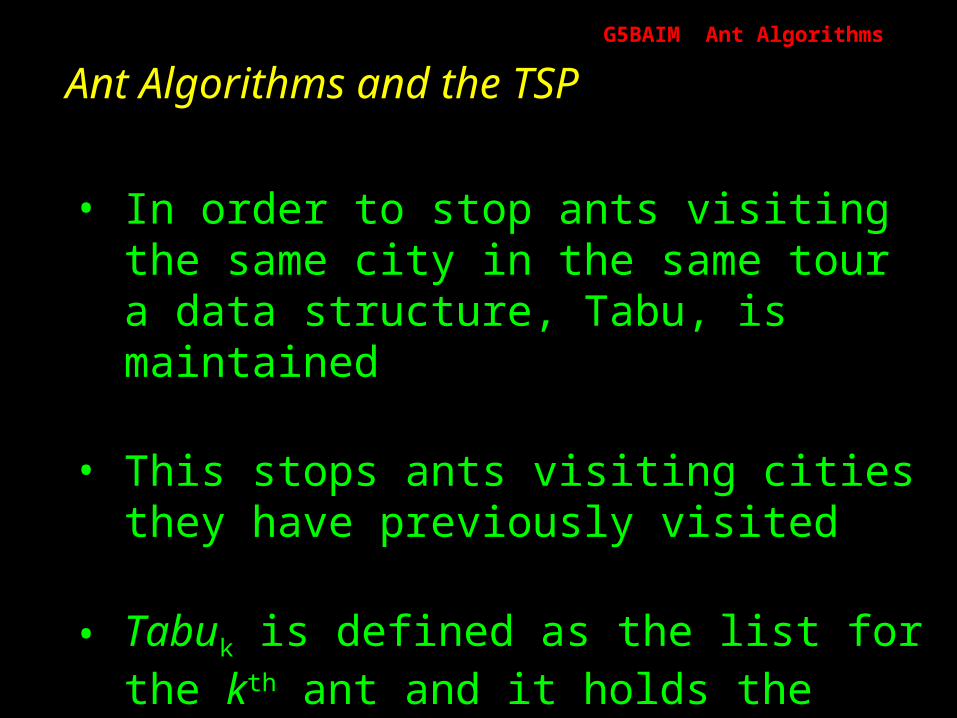
• In order to stop ants visiting the same city in the same tour a data structure, Tabu, is maintained

• This stops ants visiting cities they have previously visited

• Tabuk is defined as the list for the kth ant and it holds the cities that have already been visited



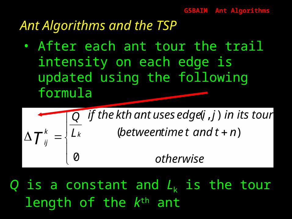
• After each ant tour the trail intensity on each edge is updated using the following formula

Tij (t + n) = p . Tij(t) + ΔTij

otherwise

ntandttimebetween

touritsinjiedgeusesantkththeif

L

Q

kk

ijT )(

),(

0

Q is a constant and Lk is the tour length of the kth ant



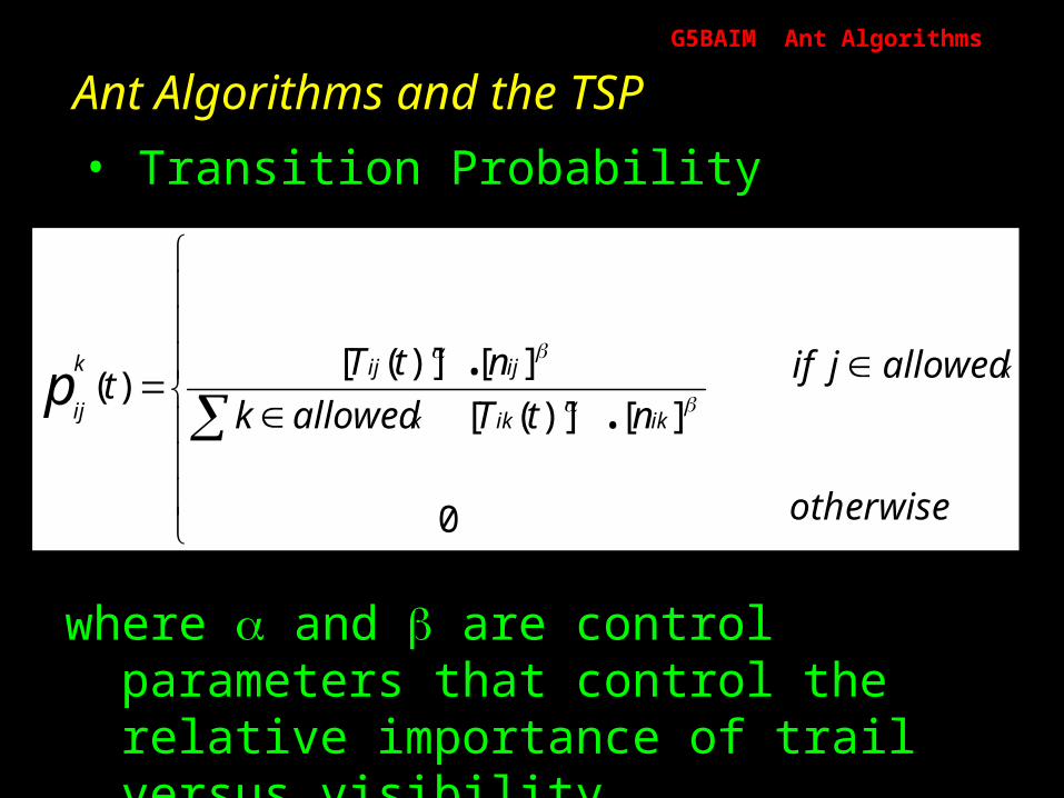
• Transition Probability

otherwise

allowedjifntTallowedk

ntTt

k

ikikk

ijijk

ijp

0

][)]([

][)]([)( .

.

where and are control parameters that control the relative importance of trail versus visibility


Ant Algorithms

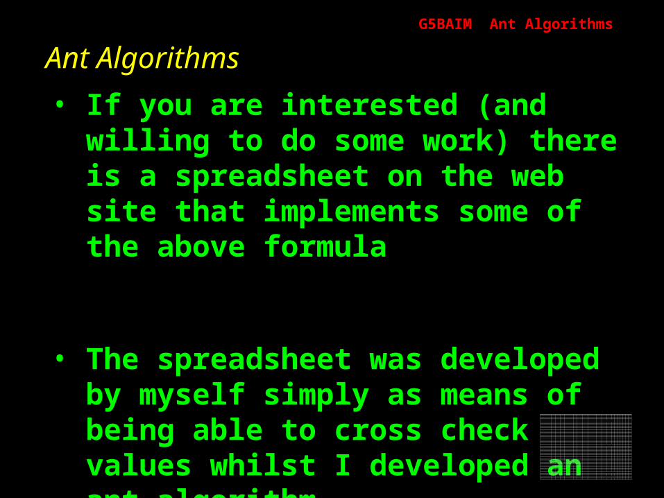
• If you are interested (and willing to do some work) there is a spreadsheet on the web site that implements some of the above formula

• The spreadsheet was developed by myself simply as means of being able to cross check values whilst I developed an ant algorithm

Numerator DenominatorMove A to A TRUE 1.73 0.00 Visibility A to A 1.00 0.00 1.73 0.00Move A to A FALSE 1.73 1.73 Visibility A to A 1.00 1.00 1.73 1.73Move A to B FALSE 1.73 1.73 Visibility A to B 0.89 0.89 1.55 1.55

Move A to B FALSE 1.73 1.73 Visibility A to B 0.89 0.89 1.55 1.55 Distance TableMove A to C FALSE 1.73 1.73 Visibility A to C 0.93 0.93 1.62 1.62 A A B B C D E FMove A to D FALSE 1.73 1.73 Visibility A to D 0.99 0.99 1.72 1.72 A 1.00Move A to E FALSE 1.73 1.73 Visibility A to E 0.77 0.77 1.33 1.33 A 1.00Move A to F FALSE 1.73 1.73 Visibility A to F 0.79 0.79 1.37 1.37 B 0.80Move A to F FALSE 1.73 1.73 Visibility A to F 0.79 0.79 1.37 1.37 B 0.80Move A to G FALSE 1.73 1.73 Visibility A to G 0.88 0.88 1.52 1.52 C 0.87Move A to H FALSE 1.73 1.73 Visibility A to H 0.98 0.98 1.70 1.70 D 0.99Move A to H FALSE 1.73 1.73 Visibility A to H 0.98 0.98 1.70 1.70 E 0.59Move A to I FALSE 1.73 1.73 Visibility A to I 0.97 0.97 1.69 1.69 F 0.63

F 0.63SUM's 22.52 20.78 11.88 10.88 20.58 18.8514898738 G 0.77

H 0.96H 0.96

Probability A to A 0.00000 I 0.95Probability A to A 0.09188

Probability A to B 0.08218 Trail Edge TableProbability A to B 0.08218 A A B B C D E FProbability A to C 0.08570 A 3.00Probability A to D 0.09142 A 3.00Probability A to E 0.07057 B 3.00Probability A to F 0.07293 B 3.00Probability A to F 0.07293 C 3.00Probability A to G 0.08062 D 3.00Probability A to H 0.09002 E 3.00Probability A to H 0.09002 F 3.00Probability A to I 0.08955 F 3.00

G 3.00H 3.00

This spreadsheet models the transition probability shown in the paper [ref12] H 3.00See notes, if necessary I 3.00

Trail Edge Constant0.5

Visibility Constant0.5


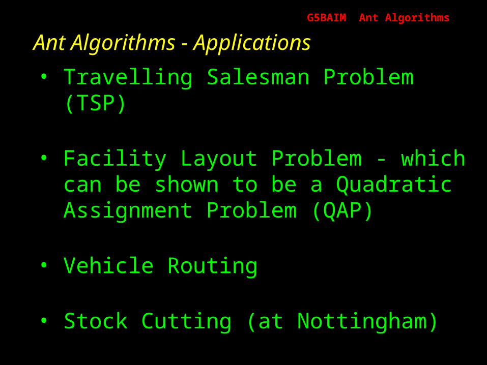
Ant Algorithms - Applications

• Travelling Salesman Problem (TSP)

• Facility Layout Problem - which can be shown to be a Quadratic Assignment Problem (QAP)

• Vehicle Routing

• Stock Cutting (at Nottingham)


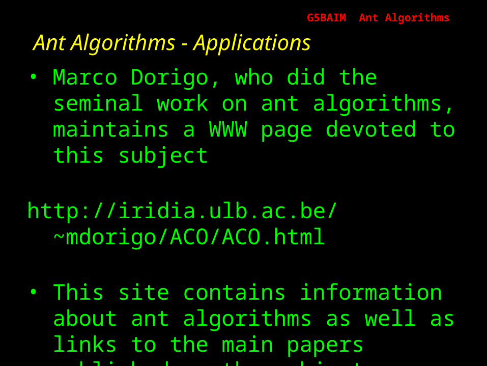
Ant Algorithms - Applications

• Marco Dorigo, who did the seminal work on ant algorithms, maintains a WWW page devoted to this subject

http://iridia.ulb.ac.be/~mdorigo/ACO/ACO.html

• This site contains information about ant algorithms as well as links to the main papers published on the subject.

G5BAIMArtificial Intelligence Methods

Graham KendallEnd of Ant Algorithms

Documents

G5BAIM Artificial Intelligence Methods Graham Kendall Ant Algorithms