Galactic noise model adjustment

Jean-Luc Vergely (ACRI-ST)

Jacqueline Boutin (LOCEAN)

Xiaobin Yin (LOCEAN)

Galactic model versus SMOS measurements

Modelled signal is underestimated. Bias of about 1 K.

Joe Tenerelli (CLS, 2011)

Aim of this study

• To better understand rugosity in L band

• To diagnose where the bias comes from

• To give leads in order to correct the bias

• To estimate the corrections for some operating points

The way to approach the galactic contribution

• Semi-empirical approach : to perform a new model.

• Formalization of the problem and simplification.

• Extraction of the reflected signal from relevant orbits.

• Estimation of the parameters of the new model.

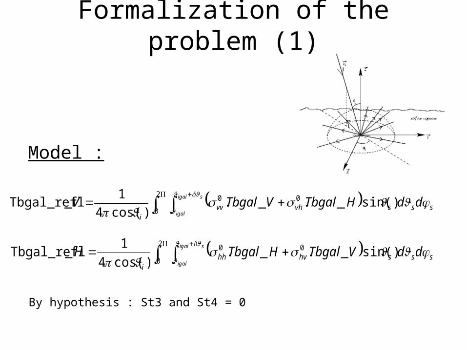
Formalization of the problem (1)

Model :

2

0

00 )sin(_._.)cos(4

1_Tbgal_refl

sigal

igalsssvhvv

i

ddHTbgalVTbgalV

2

0

00 )sin(_._.)cos(4

1_Tbgal_refl

sigal

igalssshvhh

i

ddVTbgalHTbgalH

By hypothesis : St3 and St4 = 0

Formalization of the problem (2)

Weighting by the antenna lobe :

2

0

2/

2/

''' ),()( Tbgal_refl),( _lobeTbgal_refl i

i

i iiiilobeiii ddP

Ground-antenna transformation

_sol_VTbgal_refl

_sol_HTbgal_refl

cossin

sincos

_antenne_YTbgal_refl

_antenne_XTbgal_refl22

22

aa

aa

Approximation

Assumption : Incident galactic signal is unpolarized :

Tbgal_H=Tbgal_V=Tbgal

With :

2

0)sin(,,,,_Tbgal_refl

sigal

igalsssssiissV ddTbgalAV

iissvhiissvviissV ,,,,,,,,, 00

2

0)sin(,,,,_Tbgal_refl

sigal

igalsssssiissH ddTbgalAH

iisshviissvviissH ,,,,,,,,, 00

Antenna lobe affects in theory directly the bistatic coefficients at the ground level.

Approximation : to apply antenna lobe on the galactic map.

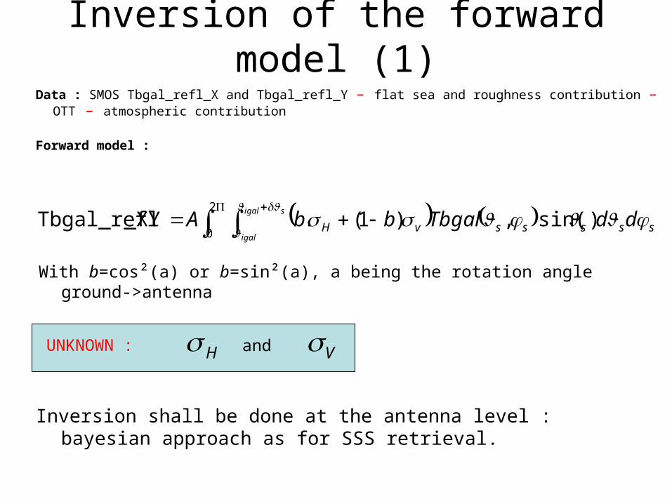
Inversion of the forward model (1)Data : SMOS Tbgal_refl_X and Tbgal_refl_Y – flat sea and roughness contribution – OTT –

atmospheric contribution

Forward model :

2

0)sin(,)1(._XYTbgal_refl

sigal

igalsssssvH ddTbgalbbA

With b=cos²(a) or b=sin²(a), a being the rotation angle ground->antenna

Inversion shall be done at the antenna level : bayesian approach as for SSS retrieval.

UNKNOWN : H and V

Inversion of the forward model (2)

Different inversion schemes :

-at small rotation angle (TB close to the track) : TBX=TBH and TBY=TBV. Possibility to retrieve independently σH and σV.

-at high rotation angle : necessity to retrieve σH and σV simultaneously

-with different parameterizations : different priors. Constraints or not on the integral. Constraint of positivity (non linear process).

-considering axisymmetric bistatic coefficients which do not depend on :

a/ WS azimuth

b/ azimuth direction of the incidence plane according to the celestial sphere.

c/ SSS and SST

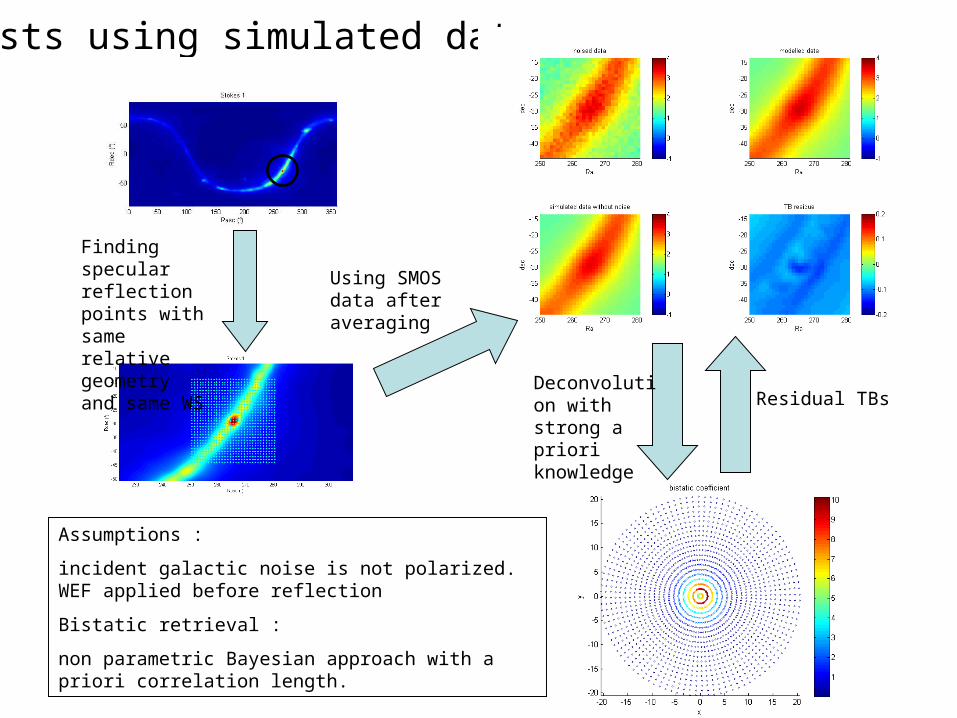
Tests using simulated data

Finding specular reflection points with same relative geometry and same WS

Using SMOS data after averaging

Deconvolution with strong a priori knowledge

Residual TBs

Assumptions :

incident galactic noise is not polarized. WEF applied before reflection

Bistatic retrieval :

non parametric Bayesian approach with a priori correlation length.

SMOS data selection

• 28 descending half orbits in the south pacific in the

period 12/09/2010 – 12/10/2010 => strong galactic signal is expected.

• Selection of data : no contamination by land, TB valid, geometric rotation < 10° : TBH and TBV processed independently.

• Place the data in (ra, dec, WS, theta) super cube : average and standard deviation in each cell of the cube.

Data presentation (1)

SMOS orbit 09/10/2010

Polar X Polar Y

SMOS orbit 09/10/2010

X polar

Theory (current model)

SMOS residues

Data presentation (2)

Y polar

Comparison of SMOS data with current model

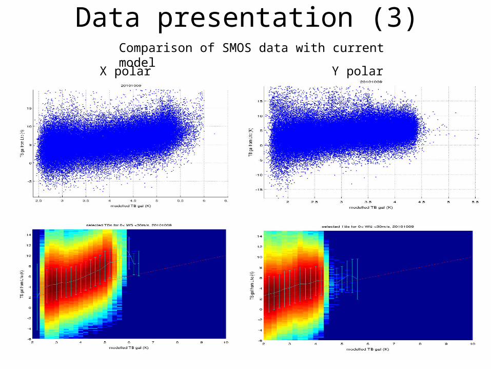
Data presentation (3)

X polar Y polar

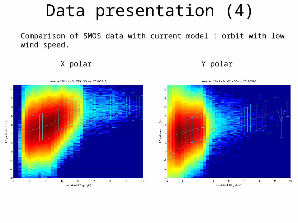
Comparison of SMOS data with current model : orbit with low wind speed.

Data presentation (4)

X polar Y polar

X polar

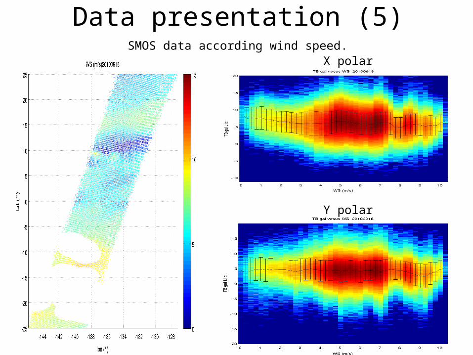
Data presentation (5)

Y polar

SMOS data according wind speed.

X polar

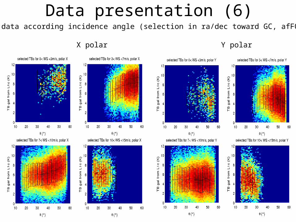
Data presentation (6)

Y polar

SMOS data according incidence angle (selection in ra/dec toward GC, afFOV)

Data presentation (7)

Definition of 20 cells in (WS, theta) space :

WS : 4 intervals [1.5m/s 4.5m/s], [1.5m/s 4.5m/s], [1.5m/s 4.5m/s], [1.5m/s 4.5m/s]

θ : 5 intervals [0° 10°], [10° 20°], [20° 30°], [30° 40°], [40° 50°]

Sampling in the (ra, dec) space : 0.5 °x 0.5 ° boxes

Cumul of 28 descending orbitsGalactic plane crosses the orbits at different x_swath positions :

12/10/201029/09/201014/09/2010

RA

DEC

Data presentation (8)Data averaging in cells. Polar X

Average data. WS = 3m/s , θ=15° Average data. WS = 6m/s, θ=45°

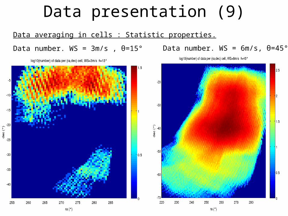
Data presentation (9)Data averaging in cells : Statistic properties.

Data number. WS = 3m/s , θ=15° Data number. WS = 6m/s, θ=45°

Data presentation (10)Data averaging in cells : Statistic properties.

Exemple of TB histogram from one cell in the cube (ra,dec,WS,theta)

Std of histogram is expected to be close to the radiometric noise. Effective std is between 2.3 and 3 K for 100 data => error of the mean is about 0.3 K

Preliminary retrieval resultspolar H

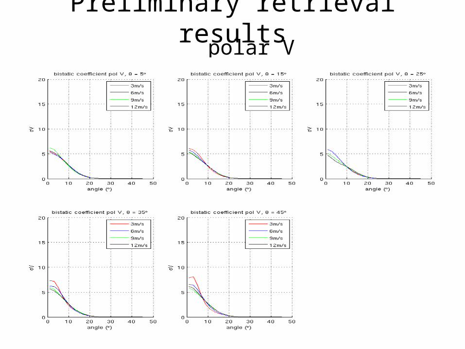
Preliminary retrieval resultspolar V

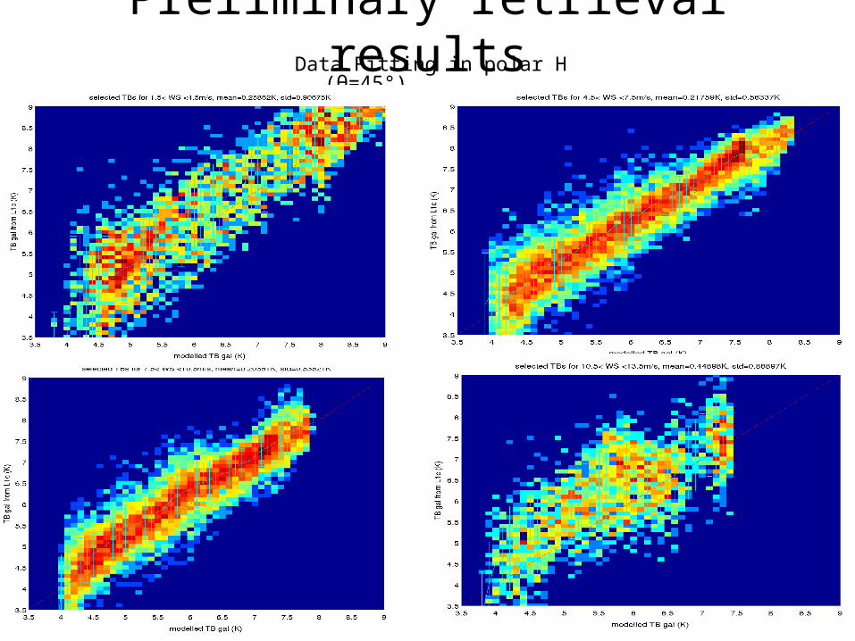
Preliminary retrieval resultsData Fitting in polar H (θ=45°)

Preliminary retrieval resultsData Fitting in polar V (θ=45°)

Preliminary retrieval results

polar H polar VReflection coefficients RH and RV

Bias in the current model : where it comes from ?

• Bias in the modelled bistatic coefficients ?• Wrong assumptions (lobe, axisymmetry) ?• Bias in the ECMWF auxiliary data (wind speed) ?• Bias in the OTT correction ?• Bias in the galactic map ?• Bias in the L1 reconstruction ?• Bias due to the target heterogeneity ?• Other sources ?