Galaxy alignment and the physical origin

Kang Xi （PMO, China) !!!

In collaboration with !

Wang Peng （PhD Student), Lin Weipeng, Yang Xiaohu, Dong X, Wang Y (SHAO)

Quy Nhon, Vietnam, July 4 2016

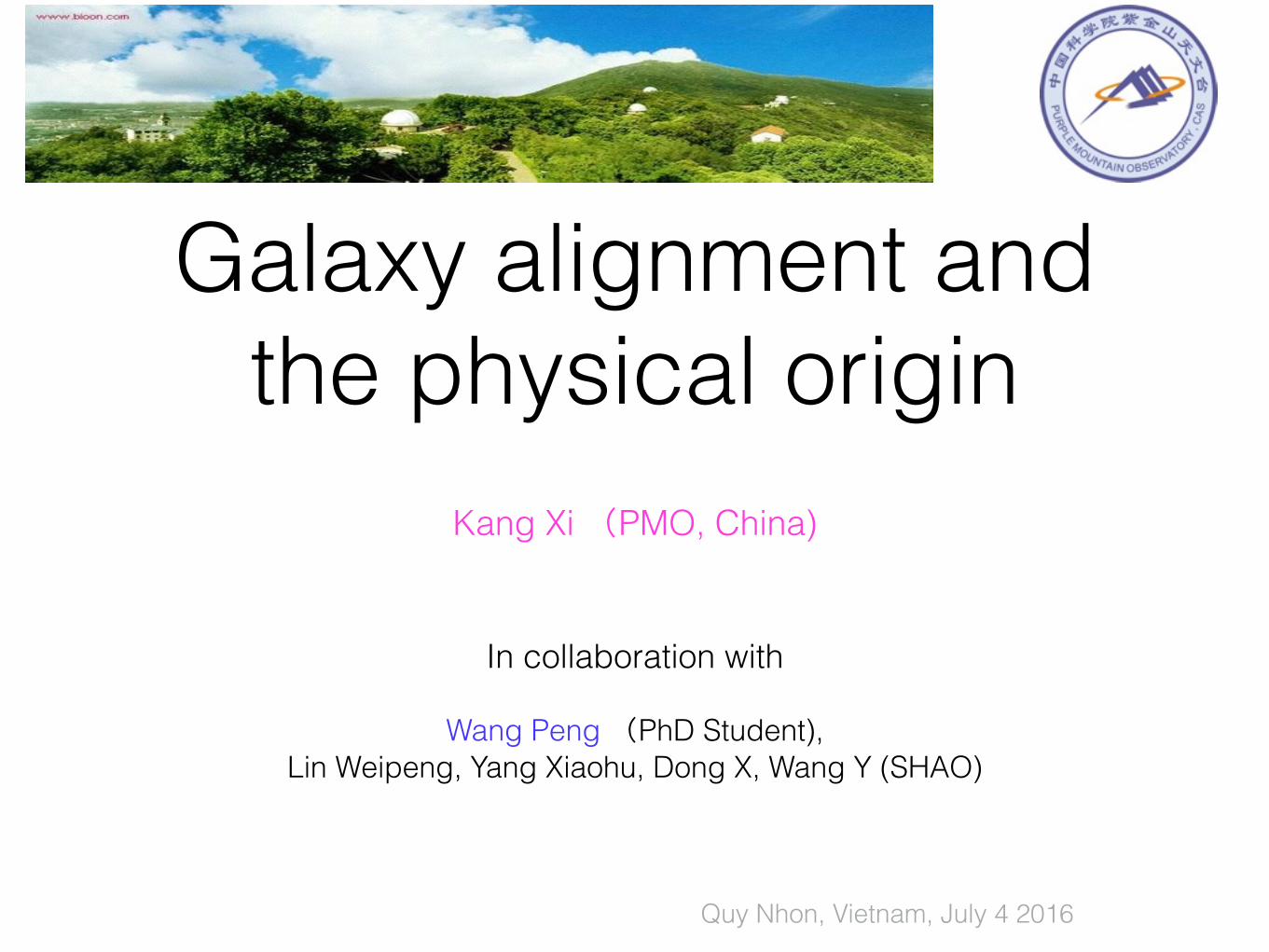
How to describe galaxy distribution in space?

in 1980,great wall 2PCF widely used for 2dFGRS/SDSS

•Correlation function: 2-points, 3-points etc (1980, Peebles) !

•2PCF describes how galaxies are biased with dark matter distribution !

•2PCF etc can well constrain the cosmological parameters

?Two-point correlation

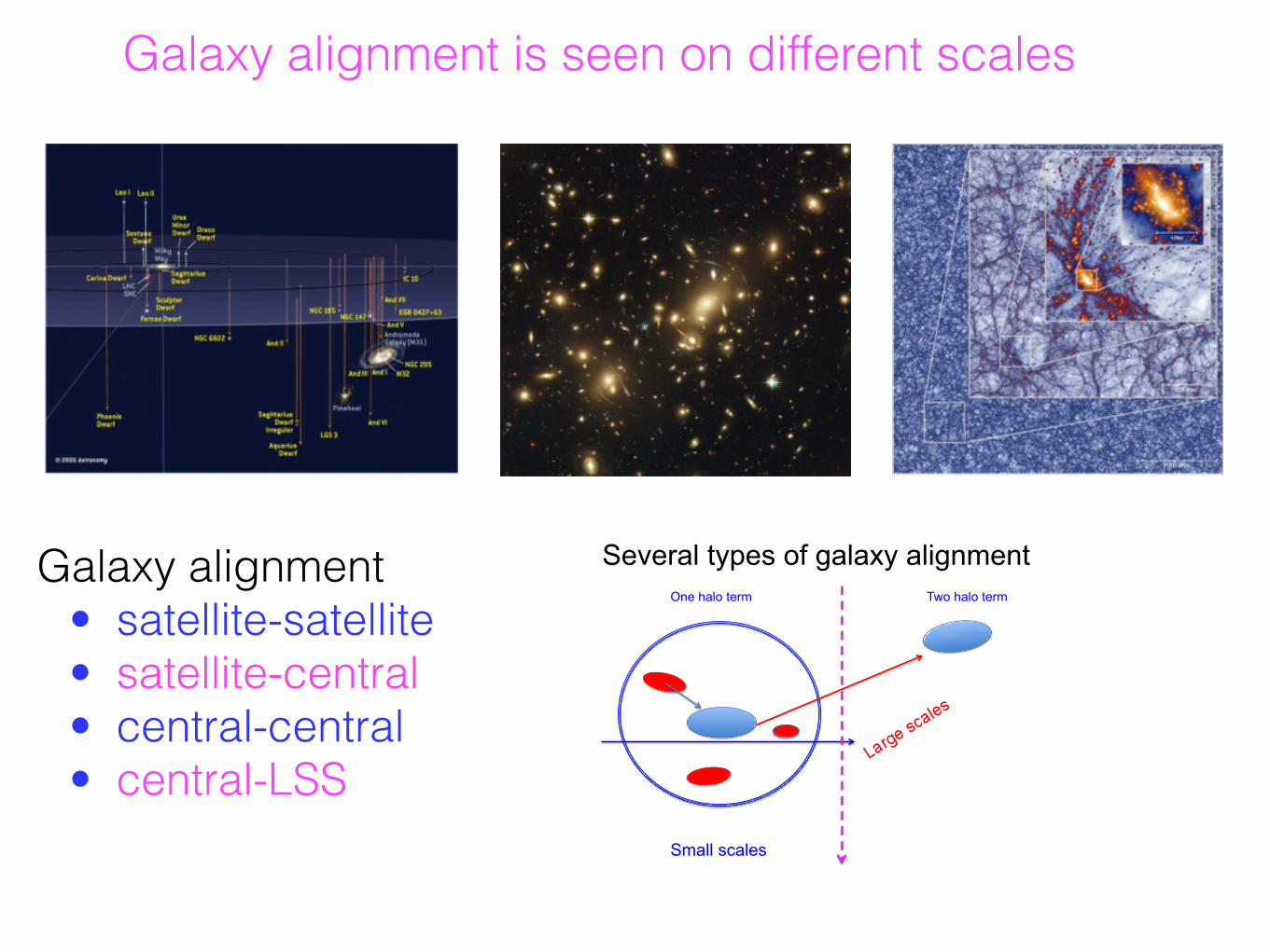
Galaxy alignment • satellite-satellite • satellite-central • central-central • central-LSS

Several types of galaxy alignment

Small scales

One halo term Two halo term

Galaxy alignment is seen on different scales

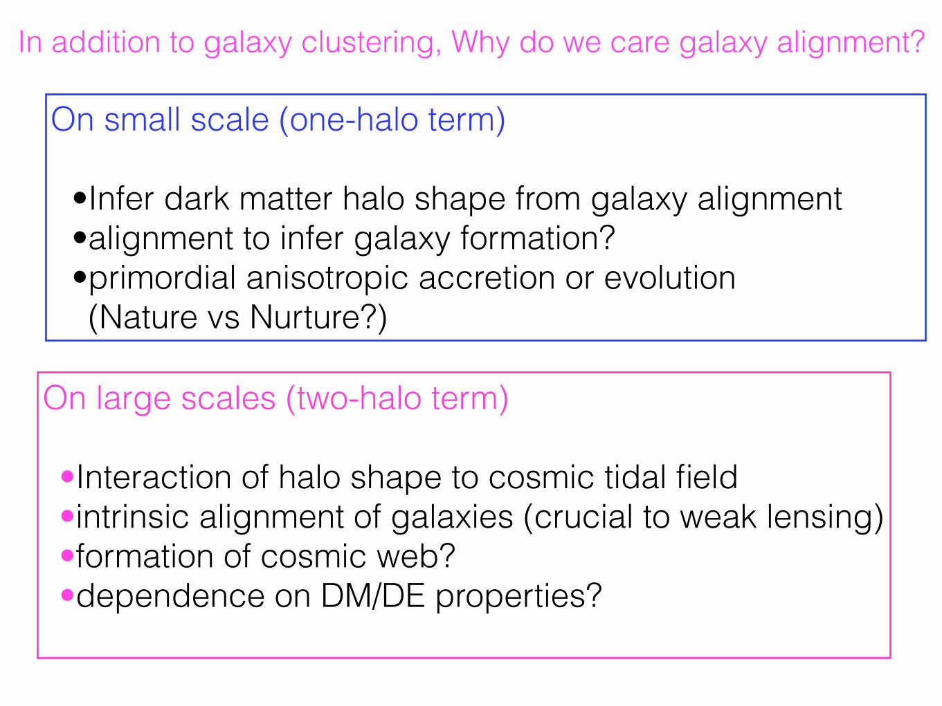
In addition to galaxy clustering, Why do we care galaxy alignment?

On small scale (one-halo term) !

•Infer dark matter halo shape from galaxy alignment •alignment to infer galaxy formation? •primordial anisotropic accretion or evolution (Nature vs Nurture?)

On large scales (two-halo term) !•Interaction of halo shape to cosmic tidal field •intrinsic alignment of galaxies (crucial to weak lensing) •formation of cosmic web? •dependence on DM/DE properties?

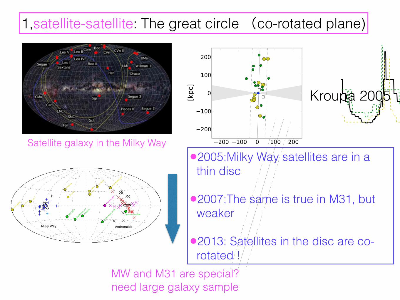
1,satellite-satellite: The great circle （co-rotated plane)

Satellite galaxy in the Milky Way12 Pawlowski, Kroupa & Jerjen

Figure 6. The distribution of LG galaxies as seen from the midpoint between the MW and M31. Note that in contrast to the previousplots, this is not plotted in Galactic coordinates l and b. Instead, the orientation of the coordinate system was chosen such that the MWand M31 lie on the equator and the normal to the plane fitted to all 15 non-satellite galaxies points to the north pole. The positionsand orientations of the MW and M31 discs are indicated by black ellipses. The Galactic disc of the MW is seen from the south, theGalactic south pole points to the upper right of the plot. Satellite galaxies are plotted as crosses (+ for MW, × for M31), non-satellitesare plotted as filled circles. The one-sigma distance uncertainties for the galaxies result in position uncertainties in this projection, whichare indicated by the grey lines. For most galaxies they are smaller than the symbols. Galaxies within a common plane are marked withthe same color. All MW satellites are assumed to lie in the VPOSall are plotted in blue, while the M31 satellites assigned to the GPoAare plotted in red. Most of the non-satellite galaxies in the LG lie along one of two ’bands’, one above and one below the plot’s centralaxis. The only LG galaxy not along one of the bands is the Pegasus dwarf irregular (dIrr). It is, however, very close to the plane of M31itself. We have indicated this by marking the satellites close to the M31 disc plane, but not in the GPoA, in magenta.

rection of (l, b) = (−136◦,−28◦), corresponding to (l, b) =(224◦,−28◦) in our notation of non-negative Galactic lon-gitude, and a plane thickness estimate of 200 kpc withoutspecifying how this thickness was measured. Using a secondmethod which assumes that the line connecting the MW andM31 lies within the LG plane, they repeat their plane fit,resulting in a plane normal pointing to (l, b) = (133◦,−27◦).As this normal direction points close to the position of M31([l, b]M31 = [121◦,−22◦]), it can not describe a plane in-cluding both the MW and M31. We therefore have to as-sume that the l-component of their second normal directionlacks a minus sign, which would agree with the statementby Pasetto & Chiosi (2007) that the difference between theirtwo planes is small. If this is the case, their second plane fitwould have a normal pointing to (l, b) = (227◦,−27◦) in ournotation. Thus, their results agree well with our plane fittedto all non-satellite galaxies in the LG.

With a RMS height of almost 300 kpc, the single planefitted to all non-satellite galaxies is much wider than thesatellite galaxy planes around the MW and M31. Motivatedby the GPoA, which consists of only a sub-sample of M31satellites, we look for the possibility that there are sub-samples of non-satellite galaxies in the LG which lie in a

thinner plane. Fig. 6 shows an Aitoff projection of the distri-bution of all LG galaxies as seen from the midpoint betweenthe MW and M31 (the origin of our Cartesian coordinatesystem). The angular coordinate system for this plot is cho-sen such that the normal-vector of the plane fitted to all15 non-satellite galaxies defines the north pole, and suchthat the MW and M31 lie along the equator at longitudesof L′ = 90◦ and L′ = 270◦, respectively. All non-satellitegalaxies are plotted as filled points in Fig. 6, the MW satel-lite positions are indicated with plus signs and those of theM31 satellites with crosses.

Galaxies which lie within a common plane that containsor passes close to the midpoint between the MW and M31will lie along a common great-circle in Fig. 6. This is, forexample, the case for the M31 satellites in the GPoA (redsymbols), because the GPoA is oriented such that it is seenedge-on from the MW and therefore also from the midpointbetween the MW and M31. Two groupings are obvious forthe non-satellites. Mostly contained in the upper half of theplot, the LG galaxies UGC 4879, Leo A, Leo T, Phoenix,Tucana, Cetus, WLM, IC 1613 and Andromeda XVI (plot-ted in yellow) lie along a common ’band’ (below, this groupwill be referred to as LGP1). A second, smaller grouping can

c⃝ 2012 RAS, MNRAS 000, 1–33

A&A 523, A32 (2010)

Fig. 4. Parameters of the MW DoS: the 3-D distribution of the MWsatellite galaxies. The 11 classical satellites are shown as large (yellow)circles, the 13 new satellites are represented by the smaller (green) dots,whereby Pisces I and II are the two southern dots. The two open squaresnear the MW are Seg 1 and 2; they are not included in the fit becausethey appear to be diffuse star clusters nearby the MW, but they do liewell in the DoS. The obscuration-region of ±10◦ from the MW disc isgiven by the horizontal gray areas. In the centre, the MW disc orienta-tion is shown by a short horizontal line, on which the position of the Sunis given as a blue dot. The near-vertical solid line shows the best fit (seenedge-on) to the satellite distribution at the given projection, the dashedlines define the region ±1.5 × ∆min, ∆min being the rms-height of thethinnest DoS (∆min = 28.9 kpc in both panels). Upper panel: an edge-onview of the DoS. Only three of the 24 satellites are outside of the dashedlines, giving Nin = 21, Nout = 3 and thus a ratio of R = Nin/Nout = 7.0.Note the absence of satellites in large regions of the SDSS survey volume(upper left and right regions of the upper panel, see also Fig. 1 in Metzet al. 2009a, for the SDSS survey regions). Lower panel: a view rotatedby 90◦, the DoS is seen face-on. Now, only 13 satellites are close to thebest-fit line, 11 are outside, resulting in R = 1.2. Note that by symmetrythe Southern Galactic hemisphere ought to contain about the same num-ber of satellites as the Northern hemisphere. Thus, The Stromlo MilkyWay Satellite Survey is expected to find about eight additional satellitesin the Southern hemisphere.

Fig. 5. Testing for the existence of the DoS. The behaviour of R for eachview of the MW, given by the Galactic longitude of the normal vectorfor each plane-fit. R = Nin/Nout is the ratio of the number of satelliteswithin 1.5× ∆min (∆min = 28.9 kpc), Nin, to those further away from thebest-fit line, Nout, calculated for all 24 known satellites, as well as forthe fits to the 11 classical and the 13 new satellites separately (takingtheir respective rms heights as the relevant ∆min). The disc-like distri-bution can be clearly seen as a strong peak close to lMW = 150◦. Notethat the position of the peaks are close to each other for both subsam-ples separately. This shows that the new satellite galaxies independentlydefine the same DoS as the classical satellite galaxies.

The fitting to the 11 classical satellites leads to results thatare in very good agreement, too. The best-fit position for the11 classical satellites is lMW = 157.◦6 ± 1.◦1 and bMW = −12.◦0 ±0.◦5, the height is found to be ∆ = 18.3± 0.6 kpc, and the closestdistance to the MW centre is DP = 8.4 ± 0.6 kpc. This is inexcellent agreement with the results of Metz et al. (2007). Inthat paper, the authors reported that lMW = 157.◦3, bMW = −12.◦7,∆min = 18.5 kpc, and DP = 8.3 kpc. This illustrates that theresults are extremely accurate despite employing a more simpledisc-finding technique.

The agreement of the fit parameters for the two subsam-ples separately is impressive. Two populations of MW satel-lite galaxies (classical versus ultra-faint) with different discov-ery histories and methods define the same DoS. This shows thatthe new, faint satellites fall close to the known, classical, DoS(≡DoScl). Even without considering the classical satellite galax-ies, the new satellites define a disc, DoSnew, that has essentiallythe same parameters. This confirms the existence of a commonDoS≈DoSnew ≈DoScl.

5.4. The DoS – discussion

A pronounced DoS is therefore a physical feature of the MWsystem. But what is its origin? Is the existence of both theclassical-satellite DoScl and the new-satellite DoSnew, such thatDoSnew ≈ DoScl, consistent with the CCM?

It has been suggested that the highly anisotropic spatial satel-lite distribution maps a highly prolate DM halo of the MW thatwould need to have its principal axis oriented nearly perpendic-ularly to the MW disc (Hartwick 2000). However, there is stillmuch uncertainty and disagreement as to the shape and orien-tation of the MW DM halo: Fellhauer et al. (2006) used thebifurcation of the Sagittarius stream to constrain the shape of

Page 12 of 22

•2005:Milky Way satellites are in a thin disc !

•2007:The same is true in M31, but weaker !

•2013: Satellites in the disc are co-rotated !

Kroupa 2005

MW and M31 are special? need large galaxy sample

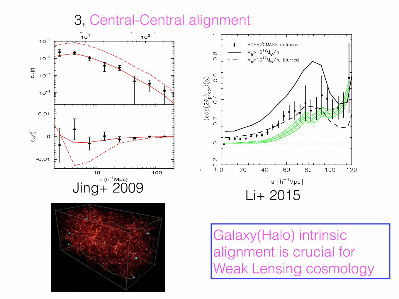
3, Central-Central alignment6 Okumura, Jing, & Li

10-4

10-3

10-2

10-1 101 102c 11

(r)Angular scale at z=1 (arcmins)

-0.01

0

0.01

10 100

c 22(r)

r (h-1Mpc)Fig. 6.— Ellipticity auto-correlation functions of the central

LRGs, (top) c11(r) and (bottom) c22(r). In both panels, the datapoints with the error bars are the measurements from the SDSS,the same ones as those in the bottom panel of Figure 1. Thedashed red lines are results of the mock central LRGs with nomisalignment with their parent halos. The solid red lines are thosewith the misalignment parameter of σθ = 35◦. The horizontalaxis at the top shows the corresponding angular scale when all thegalaxies are located at z = 1.

mock ellipticity catalogs are not independent each other,their average can reduce random fluctuation from differ-ent random seeds. Finally, our model prediction for eachmisalignment parameter σθ is calculated by averagingover 7 × 9 = 63 misaligned samples.

In comparing the observational data with the modelprediction, we first compute the model ellipticity corre-lation function with a given parameter of σθ to be tested.χ2 statistics are then calculated as

χ2(σθ) =!

i,j

∆c11(ri; σθ)C−1ij ∆c11(rj ; σθ), (7)

where Cij is the covariance matrix given by equation(3), ∆c11(ri; σθ) the difference between the observed andthe model values in the ith separation bin, and i andj runs over the number of bins. In this analysis thenumber of bins is 8 and the degree of freedom is 7. Thusthe 99 realizations constructed from jackknife resamplingare large enough to derive a nonsingular matrix, as wasalready stated in Section 3.1. The range of σθ in ourcalculation of χ2 is 20 < σθ < 50◦ with the width of∆σθ = 1◦. The binned values of χ2 are then cubic-splineinterpolated.

5

10

15

20

30 35 40 45

χ2

Misalignment parameter (deg)

full covariancediagonals only

5

10

15

20

30 35 40 45

χ2

Misalignment parameter (deg)

full covariancediagonals only

Fig. 7.— χ2 distribution for misalignment angle parameter σθ.The best-fit parameter is σθ = 35.4+4.0

−3.3 deg (68% C.L.) when we

use the full covariance matrix, while σθ = 35.0+4.4−3.6 deg when we

use only the diagonal elements of the covariance. The minimumvalue of χ2 is χ2

min= 3.983 and 2.915 with 7 dof, respectively.

The horizontal dotted lines show 68%, 95%, and 99% confidencelevels.

Figure 7 shows χ2 as a function of the misalignmentparameter σθ. For comparison, both the results that allthe elements and only diagonals of the covariance ma-trix are used are given. These two results are in verygood agreement, indicating that the non-diagonal ele-ments of the error matrix are not important. The fits ofthe observed ellipticity correlation function to the modelprediction using the full covariances give σθ = 35.4+4.0

−3.3

(68% confidence level), and χ2min = 3.983 with 7 dof.

The model prediction of c11 with σθ = 35◦ is shown inthe top panel of Figure 6. As a cross-check, we also plotthe model of c22 with the same σθ in the bottom panelof Figure 6, which is also in very good agreement withthe observed c22. This accordance additionally enhancesthe validity of our analysis.

Recently there were two papers by Kang et al. (2007)and Wang et al. (2008) who studied the misalignmentangle between galaxies and their host halos. Althoughthey used the same observed statistics of the alignmentangle between the major axis of the central galaxiesand their connecting lines to satellites(Yang et al. 2006),they obtained the typical misalignment angle with dif-ferent results (about 40◦ by Kang et al. (2007) and 23◦

by Wang et al. (2008) for the whole sample of blue andred central galaxies in their papers). The difference maycome from their different methods to trace the satel-lite spatial distribution in their modeling. Kang et al.(2007) have used a semi-analytical model to trace satel-lites, and Wang et al. (2008) have first tried to determinethe spatial distribution of satellites within halos. Thediscrepancy might come from the fact that the triaxialshape of satellite distribution within groups determinedby Wang et al. (2008) is much rounder than dark mat-ter halos in simulations (Jing & Suto 2002; Kang et al.2007). Our analysis does not need to make any assump-tion for the satellite galaxies or the shape of halos. Be-

Jing+ 2009

Large scale alignment of massive galaxies at z ∼ 0.6 3

Fig. 1.— Left: difference between the alignment correlation function at given projected angle ξ(θp, s) and the conventional correlationfunction ξ(s), obtained from the CMASS galaxy sample. Results at the small and large θp bins are plotted in grey and black symbolsseparately. The hatched regions plotted in red/green/blue represent the 1σ variance between 100 random samples in which the positionangles are randomly shuffled among the galaxies, measured for the three angle bins separately. The solid and dashed lines show the resultsfor dark matter halos with mass above 1012h−1M⊙. The solid lines are for the halos with no misalignment, and the dashed lines are resultswith the misalignment parameter of σθ = 35◦. Right: the cos(2θ)−statistic measured for the same galaxy sample and dark matter halocatalog. Symbols and lines are the same as in the left-hand panel.

only the redshift-space separation and can be regardedas an average of the alignment correlation function overthe full range of θp.In Figure 1 (left panel) we plot the difference in the

alignment correlation function at small/large angles withrespect to the conventional correlation function ξ(s).The error bars plotted in the figure and in what followsare estimated using the bootstrap resampling technique(Barrow et al. 1984). We have constructed 100 bootstrapsamples based on the real sample, and we estimate thedifference between ξ(θ, s) and ξ(s) for each sample. Theerror at given scale is then estimated from the 1σ vari-ance between the bootstrap samples.As can be seen, ξ(θp, s) differ from ξ(s) at both small

and large angles, with stronger clustering at smaller an-gles and weaker clustering at larger angles, consistentwith the picture that the major axis of the galaxies ispreferentially aligned with their spatial distribution.It is essential to perform systematics tests on any

clustering measurements (e.g. Mandelbaum et al. 2005;Sanchez et al. 2012). As one of such tests, we have re-peated the same analysis as above for a set of 100 ran-dom samples in which the position angles are shuffledat random among the main galaxies (Sample Q). Thehatched regions plotted in red/green/blue in Figure 1show the 1σ variance of the alignment correlation func-tion between the random samples, measured for the threeangle bins separately. It is interesting that the alignmentsignal detected in the real sample is significantly seen fora wide range of scales, from the smallest scales probed(∼ 5h−1Mpc) out to ∼ 70h−1Mpc according to both thebootstrap errors of the measurements and the 1σ regionsof the random samples.The right-hand panel of Figure 1 shows the

cos(2θ)−statistic, plotted in solid circles for the CMASSsample and in green hatched region for the 100 randomlyshuffled samples. The statistic for the real sample showspositive values on all scales probed, while its differencefrom the random samples is significantly seen only forscales below ∼ 70h−1Mpc, consistent with what the left-hand panel reveals. As mentioned above, a positive valuein the cos(2θ)−statistic indicates a preference for anglessmaller than 45◦, thus implying that the major axis ofthe galaxies tends to be aligned with the large-scale dis-tribution of galaxies. The cos(2θ)−statistic of the ran-dom samples shows a systematic positive bias at scalesabove ∼ 40h−1Mpc, implying that the position angle ofthe CMASS galaxies is not randomly distributed on thesky, a cosmic variance effect due to the limited surveyarea and probably also the quite irregular shape of thesurvey geometry. This can be tested in future with mockcatalogs or later data releases of the BOSS survey.For comparison the same statistics obtained for dark

matter halos of mass Mh > 1012h−1M⊙ in the MDR1simulation are shown in Figure 1 as solid lines. Align-ment signal is seen in both statistics and on all thescales up to 120 h−1Mpc. Both statistics show strongdependence on the spatial scale, which is very simi-lar to what is seen for the CMASS galaxies. At fixedscale, however, the alignment of the halos is system-atically stronger than that of the galaxies. This dis-crepancy might be partially (if not totally) due to themisalignment between the orientation of central galaxiesand that of their host halos. A previous study done byOkumura et al. (2009) on the alignment of luminous redgalaxies (LRGs) at 0.16 < z < 0.47 in the SDSS/DR6suggested that the misalignment angle between a centralLRG and its host halo follows a Gaussian distribution

Li+ 2015

Galaxy(Halo) intrinsic alignment is crucial for Weak Lensing cosmology

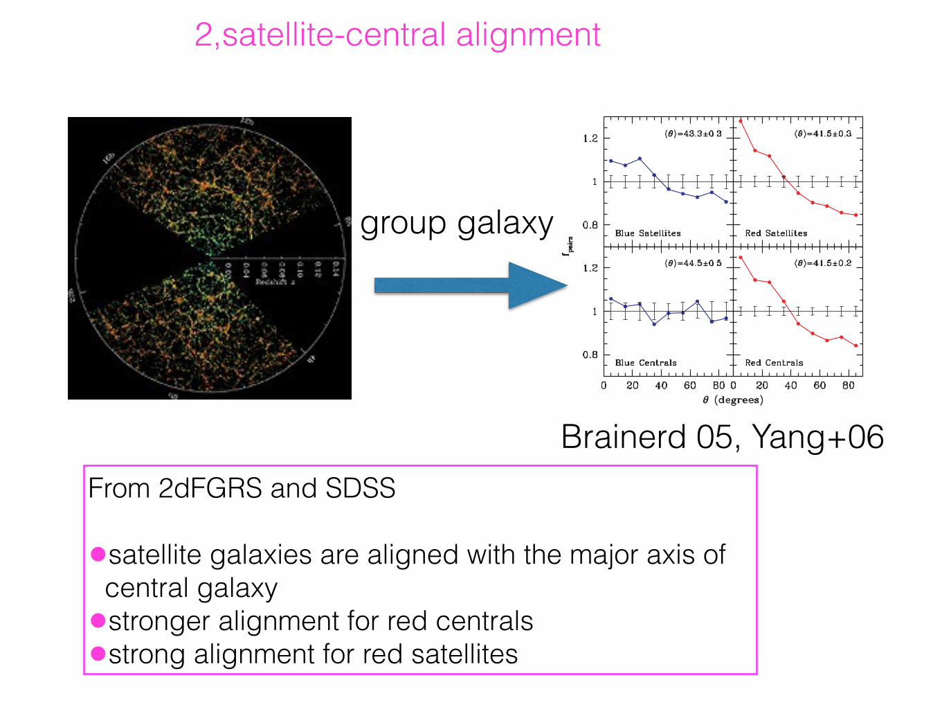
2,satellite-central alignment

The central-satellite alignment 1297

Figure 2. Same as Fig. 1 but for different subsamples of central and satellite galaxies. In the upper panels, we show f pairs(θ ) for groups with a different

ellipticity, e, of the central galaxy, as indicated. Note that groups with a strongly elongated central galaxy (0.6 ! e < 0.8) are consistent with a perfectly

isotropic distribution of satellites. As we argue in the text, and show in Fig. 3, this owes to the fact that strongly elongated systems are mainly blue, late type

disc galaxies, which show no significant alignment. The lower panels show how f pairs(θ ) depends on the luminosities of the satellite galaxies, Ls, expressed

in units of the luminosity of their central galaxy, Lc. There is a clear indication that fainter satellites are more strongly aligned.

Figure 3. Same as Fig. 1, but for different subsamples of hosts and satellites,

selected according to their 0.1(g − r ) colour. See text for discussion.

galaxies. In particular, satellite galaxies in groups with a blue, central

galaxy are consistent with a perfectly isotropic distribution; there

is no sign of any significant alignment (⟨θ⟩ = 44.◦5 ± 0.◦5). On the

contrary, groups with a red central galaxy show a very pronounced,

major-axis alignment with ⟨θ⟩ = 41.◦5 ± 0.◦2. In addition, red satel-

lites show a significantly stronger major-axis alignment than blue

satellites.

As shown in Weinmann et al. (2006), haloes with a central red

galaxy have a significantly larger fraction of red satellites than a

halo of the same mass, but with a blue central galaxy. This so-called

‘galactic conformity’ implies that the upper and lower panels are

not independent. In Fig. 4, we therefore examine how f pairs(θ ) de-

Figure 4. Same as Fig. 3, except that here we split the sample according to

the colours of both the central and the satellite galaxies, as indicated.

pends on the colours of both the central galaxy and the satellites.

As can be seen, systems with a blue central galaxy show no sig-

nificant alignment, neither with their blue satellites nor with their

red satellites. Systems with a red central galaxy, however, show a

very pronounced alignment, which is significantly stronger for red

satellites than it is for blue satellites. Since redder colours typically

indicate older stellar populations, these results suggest that a sig-

nificant alignment between the orientation of central galaxies and

the distribution of their satellite galaxies only exists in haloes with a

relatively old stellar population. Clearly, such a correlation between

the alignment strength and the age of the stellar population must

C⃝ 2006 The Authors. Journal compilation C⃝ 2006 RAS, MNRAS 369, 1293–1302

From 2dFGRS and SDSS !•satellite galaxies are aligned with the major axis of

central galaxy •stronger alignment for red centrals •strong alignment for red satellites

Brainerd 05, Yang+06

group galaxy

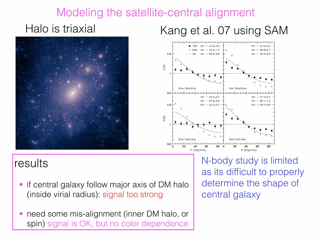
Modeling the satellite-central alignmentHalo is triaxial

Alignment between satellites and centrals 1535

Figure 2. The normalized probability distribution P(θ ) for central–satellitepairs in VIR haloes at different redshifts, as indicated. Clearly, the alignmentstrength in the SAM is virtually independent of redshift.

Figure 3. The normalized probability distribution, P(θ ), for various subsamples. The upper panels show the results for blue (left-hand panel) and red (right-handpanel) satellites, while the lower panels show the results for haloes with blue centrals (left-hand panel) and red centrals (right-hand panel). In each panel, theopen triangles show the results for the satellite galaxies in the SAM, the solid line shows the results for the dark matter particles in the SAM and the solid dotswith error bars show the observational results of Y06.

3.2 Dependence on galaxy colour

We now examine how the alignment signal depends on variousgalaxy and halo properties. Fig. 3 shows the dependence of the align-ment signal on the colours of the satellite galaxies (upper panels)and the central galaxies (lower panels). The open triangles show theresults obtained from our SAM, while the observational results ofY06 are shown as solid dots. Similar to the results shown in Fig. 1,the SAM yields much stronger alignment signals than observed.Again we defer the discussion of this difference and its implicationsto Section 4. Here we simply focus on the colour dependence. Firstof all, the SAM predicts that blue satellites are less strongly alignedwith the orientation of their central galaxy than red satellites, whichis in qualitative agreement with the observations. The solid linesindicate the P(θ ) for the dark matter particles. This shows that bluesatellites have a θ distribution that is virtually identical to that of thedark matter particles, while red satellites reveal an alignment signalthat is clearly enhanced with respect to that of the dark matter.

In order to gain insight in the origin of this enhanced align-ment signal of red satellites, we have inspected the galaxy distri-butions in the SAM. This shows that red satellites are more radiallyconcentrated than the blue satellites, in agreement with observa-tions (e.g. Postman & Geller 1984; Girardi et al. 2003; Biviano &Katgert 2004; Thomas & Katgert 2006). In addition, we find thatblue satellites are mostly associated with halo galaxies (the satel-lites that still have a detectable subhalo around them). This owes tothe fact that most of them have been accreted only fairly recently.Red satellites, on the other hand, have their star formation largely

C⃝ 2007 The Authors. Journal compilation C⃝ 2007 RAS, MNRAS 378, 1531–1542

by guest on July 7, 2015http://m

nras.oxfordjournals.org/D

ownloaded from

Kang et al. 07 using SAM

results !• if central galaxy follow major axis of DM halo

(inside virial radius): signal too strong !

• need some mis-alignment (inner DM halo, or spin) signal is OK, but no color dependence

N-body study is limited as its difficult to properly determine the shape of central galaxy

Modeling the satellite-central alignment

Satellite Alignment 3

0.8

0.9

1.0

1.1

1.2

1.3

p(θ

)

< θ >model= 42.1±0.1< θ >obs= 42.2±0.2All Sample

< θ >model= 42.4±0.3< θ >obs= 43.3±0.3Blue SGs

< θ >model= 42.1±0.1< θ >obs= 41.5±0.3Red SGs

0 10 20 30 40 50 60 70 80θ

0.8

0.9

1.0

1.1

1.2

1.3

p(θ

)

< θ >model= 42.0±0.1< θ >obs= 44.5±0.5Blue CGs

0 10 20 30 40 50 60 70 80θ

< θ >model= 43.2±0.2< θ >obs= 41.5±0.2Red CGs

0 10 20 30 40 50 60 70 80θ

CGs De f ined By Halo Mass

Mh < 2∗1011M⊙

Mh < 1012M⊙

Mh > 2∗1011M⊙

Mh > 1012M⊙

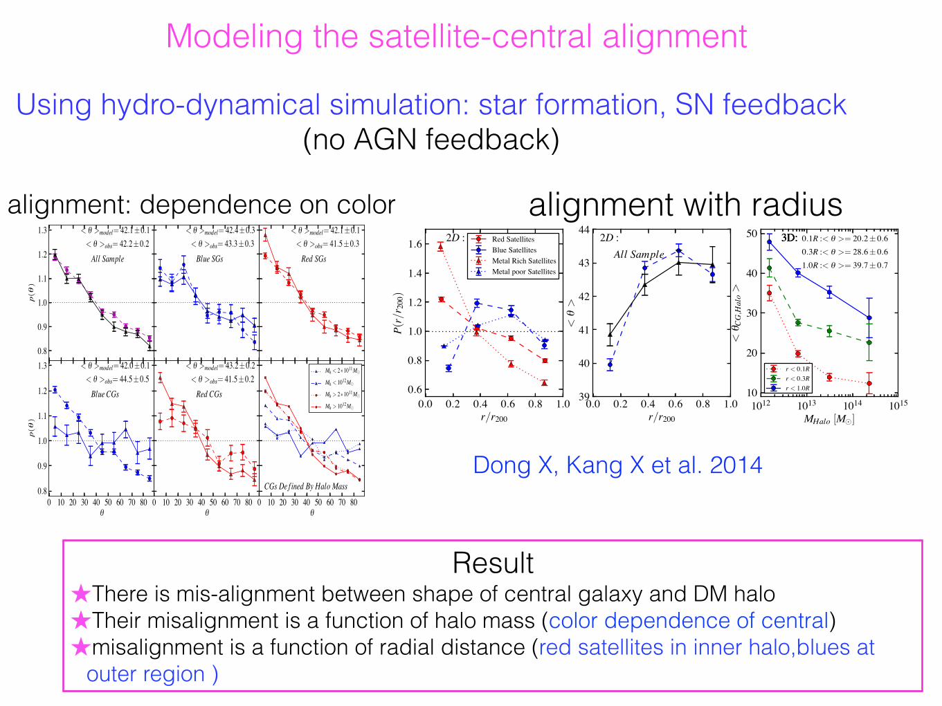
FIG. 2.— The predicted galaxy alignment and comparisons with observa-tional results.The upper left panel is for all sample, and lower right panel forcentral galaxies with different host halo mass. Other panles are for satelliteand central with red/blue colors. The average alignment angle of observedand model galaxies are labeled in each panel.

right panel we show the predicted alignment for red/blue cen-tral galaxies divided by Mc, where Mc = 2× 1011M⊙ (dottedline), and Mc = 1012M⊙ (dashed line). It is found that the pre-dicted alignment is close to the data with Mc = 2× 1011M⊙,and the prediction is increasing with critical halo mass.

The exersie presented in the lower right panel of Fig.2 sug-gests that the observed alignment with dependence on color ofcentral galaxies is mainly determined by the host halo mass.We will later see that the halo mass dependence is rootedin the shape correlation between central galaxy and the hosthalo.

In Fig.3, we further show the dependence of alignment ongalaxy properties from the simulation. The solid lines are forcentrals and dashed lines for satellites with dependence onmetallicity, color, stellar mass and halo mass. The upper pan-els show that the alignment of satellites depends on metallicityand color, with stronger dependence on metallicity that metal-rich satellites have very strong alignment. The lower panelsshow that the dependence on stellar mass is very weak andfainter satellites have slightly weaker alignment, in a broadagreement with the finding in Y06. Note the error-bar for thepoint at the bin with biggest mass is big due to small num-ber statistics. The halo mass dependence in the lower rightpanel is close to the dependence from the data that alignmentin massive halos are stronger and consistent with the depen-dence on stellar mass for central galaxies in the left panel.

In addition to the dependence of galaxy alignment on color,the data also have shown that the alignment angle is a strongfunction of radial distance to the centrals (Brainerd 2005;Yang et al. 2006). In the left panel of Fig.4 we show the radialspatial distribution of satellite in the dark matter halo, with de-pendence on color and metal. It is found that both metal richand red satellites are distributed predominately in the centralhalo. This distribution agrees with the observational facts thatgalaxy properties, such as color, metallicity or morphologydepends strongly on its environment/local density as metal re-cycle and star formation quenching are more efficient in theinner halo (ref?). The middle panel in Fig.4 shows the align-ment of satellites as function as radius. The observational re-sults of Y06 is shown as triangles. Good agreement betweenthe simulation and the data is found that satellites residing ininner halo have stronger alignment with central galaxy than

FIG. 3.— The dependence of alignment strength (2D) on the properties ofsimulated galaxies and dark matter halos. See the text for more details.

FIG. 4.— Left panel: The radial distribution of red and blue SGs withindark matter halos. Middle panel: The dependence of average alignment angleon radii toward halo center. Right panel: The distribution of mis-alignmentangles between the major axis of CGs and that of dark matter halo withinradius of 0.1, 0.3 and 1.0R200.

their counterparts residing in outer halo.To understand the origin of satellite alignment with respect

to the central galaxy, theoretical work using N-body simula-tion often assumed that the shape of central galaxy followsthe overall dark matter halo, and that leads to a strong align-ment than the data (e.g., Kang et al. 2007). To decrease thepredicted signal, one has to introduce some degree of mis-alignment between the central galaxy and that of the darkmatter halo without resort to the physical origin (Kang et al.2007; Agustsson & Brainerd 2010). More physical solution isproposed that if the central galaxy follows better the shape ofdark matter in the central region, the alignment will be betterreproduced (Faltenbacher et al. 2009; Wang et al. 2014), how-ever the dependence on galaxy color is hardly reproduced inthese works.

As our SPH simulation includes the stellar component, wecan directly predict the shape of central galaxy and is able totest the above assumption. The right panel of Fig.4 shows thealignment angle between central galaxy and dark matter ha-los with dependence on halo mass. The results for the anglebetween the major axis of central galaxy and the overall darkmatter halo were plotted as solid line, dashed line and dot-ted line for the whole halo (inside of R200), the intermediatehalo (inside of 0.3R200) and the inner halo (inside of 0.1R200)respectively. Here R200 is the virial radius of spherical halo.It is found that the shape of central galaxy traces better thatof the inner halo, and this alignment is increasing with halomass. The mean mis-alignment angle varies from ∼ 35 − 10

Using hydro-dynamical simulation: star formation, SN feedback (no AGN feedback)

Alignment of Satellite Galaxies 5

0.0 0.2 0.4 0.6 0.8 1.0r/r200

0.6

0.8

1.0

1.2

1.4

1.6

P(r/r 200)

2D : Red SatellitesBlue SatellitesMetal Rich SatellitesMetal poor Satellites

0.0 0.2 0.4 0.6 0.8 1.0r/r200

39

40

41

42

43

44

<θ>

2D :All Sample

1012 1013 1014 1015MHalo [M⊙]

10

20

30

40

50

<θ C

G,Halo>

3D: 0.1R :< θ >= 20.2± 0.63D:0.3R :< θ >= 28.6± 0.6

3D:

1.0R :< θ >= 39.7± 0.7

r < 0.1Rr < 0.3Rr < 1.0R

FIG. 4.— Left panel: radial distribution of red and blue, metal-rich (top 30% by order ranking), and metal poor (bottom 30% by order ranking) SGs within darkmatter halos. Middle panel: dependence of average alignment angle on radius from the halo center. Right panel: distribution of mis-alignment angles betweenthe major axes of CGs and those of dark halos measured within radii of 0.1, 0.3, and 1.0R200.

follow that of dark matter. On the other hand, the stellar com-ponent of centrals is also greatly shaped by the gravitationalforce of the dark matter in the inner halo. The combinationof these two effects leads to a better alignment for the metal-rich/red satellites than their metal-poor/blue counterparts. Asto the dependence on color of centrals, this is related to thehalo mass of the centrals – bluer centrals most likely reside inrelatively lower-mass halos where the alignment between thecentral stellar component and the inner halo shape becomesweaker.

4. CONCLUSION AND DISCUSSIONIn this Letter, we carry out a study of galaxy alignment us-

ing a cosmological simulation including gas cooling, star for-mation, and supernova feedback, which enables a direct pre-diction for the shape of CGs and the galaxy properties. Wefind that the predicted alignment between the CG and the dis-tribution of satellites agrees with the observations. Further-more, with a simple assumption about the halo mass of blueand red centrals, the dependence on color for both centralsand satellites is also reproduced. We also identify that thestrongest dependence of the alignment is with metallicity ofsatellites, which should be testable using future data.The main source of galaxy alignment is the non-spherical

nature of CDM halos, as shown by many previous stud-ies (e.g., Agustsson & Brainerd 2006a,b; Kang et al. 2007).However, the predicted strength of the alignment is too strongif the shape of the CG follows the overall shape of the darkmatter halo. From our study, we find that the shape of the CGbetter follows the halo in the inner region, and the averagemis-alignment is about 20deg (see Figure 4), similar to the ex-pected or inferred values in previous studies (e.g., Wang et al.2008; Faltenbacher et al. 2009). As the most red/metal-richsatellites stay in the inner halo, they naturally follow theshape of the dark matter halo in that region. This leads toa strong alignment between red satellites with centrals. Fur-thermore, as the alignment between the CG and inner halo

increases with halo mass and red centrals predominately pop-ulate massive halos, it explained the observed fact that redcentral shows stronger alignment with satellites than blue cen-trals. Although the prediction for the alignment of blue cen-trals using our simulation fails because of the too blue col-ors of the most massive central galaxies, the exercises for thealignment dependence on halo mass have given hints that sim-ulations with AGN feedback (e.g., Vogelsberger et al. 2013;Tenneti et al. 2014) should be helpful to solve this problem.The non-spherical nature of dark matter halos is one the

most prominent features of structure formation in a CDM uni-verse, as the mass accretion and mergers predominately occuralong the cosmic web or the filament (e.g., Wang et al. 2005).It also naturally produces the galaxy alignment on very largescales up to ∼ 70h−1Mpc (Li et al. 2013). Accurate predic-tions for galaxy alignment on large scales is crucial to cosmo-logical applications, such as estimating the systematic errorused in weak lensing measurements. With the proper mod-eling of galaxy shapes from hydrodynamical simulation, wewill be able to make predictions for galaxy alignment on largescales in a forthcoming paper.

The authors thank the anonymous referee for useful sugges-tions. W.P.L. and X.K. acknowledge supports by the NSFCprojects (No. 11121062, 11233005, U1331201, 11333008)and the “Strategic Priority Research Program the Emergenceof Cosmological Structures” of the Chinese Academy ofSciences (grant No. XDB09010000). X.K. is also sup-ported by the National basic research program of China(2013CB834900) and the foundation for Distinguished YoungScholars of Jiangsu Province (No. BK20140050) . Thesimulations were run in the Shanghai Supercomputer Cen-ter and the data analysis was performed on the supercomput-ing platform of Shanghai Astronomical Observatory. X.K.,A.A.D. and A.V.M., acknowledge support from the MPG-CAS through the partnership program between the MPIAgroup lead by A.Macciò and the PMO group lead by X. Kang.

REFERENCES

Agustsson, I., & Brainerd, T. G. 2006a, ApJ, 650, 550Agustsson, I., & Brainerd, T. G. 2006b, ApJL, 644, L25Agustsson, I., & Brainerd, T. G. 2010, ApJ, 709, 1321Bahl, H., Baumgardt, H., 2014, MNRAS, 438, 2916Bailin, J., Power, C., Norberg, P., et al., 2008, MNRAS, 390, 1133Baldry, I.K., Balogh, M.L., Bower, R.G., et al., 2006, MNRAS, 373, 469Brainerd, T. G. 2005, ApJL, 628, L101Bruzual, G., & Charlot, S. 2003, MNRAS, 344, 1000

Cattaneo, A., Dekel, A., Faber, S. M., & Guiderdoni, B. 2008, MNRAS,389, 567

Chabrier, G., 2003, PASP, 115, 763Deason, A. J., McCarthy, I. G., Font, A. S., et al. 2011, MNRAS, 415, 2607Faltenbacher, A., Li, C., Mao, S., et al. 2007, ApJL, 662, L71Faltenbacher, A., Li, C., White, S. D. M., et al. 2009, RAA, 9, 41Font, A. S., McCarthy, I. G., Crain, R.A., et al., 2011, MNRAS, 416, 2802Grebel, E.K., & Guhathakurta, P., 1999, ApJL, 511, L101Holmberg, E. 1969, ArA, 5, 305

alignment: dependence on color alignment with radius

Dong X, Kang X et al. 2014

Result ★There is mis-alignment between shape of central galaxy and DM halo ★Their misalignment is a function of halo mass (color dependence of central) ★misalignment is a function of radial distance (red satellites in inner halo,blues at

outer region )

Zel’dovich approximation for formation of cosmic web

8 Cautun et al.

Figure 2. The formation of structure according to the Zel’dovichformalism. The sequence starts with the left most panel whichshows an ellipsoidal overdensity from two perpendicular angles.The overdensity collapse proceeds most strongly along one axisto form a sheet, followed by the full contraction of the second axisto form a filament. At last, full collapse takes place resulting in a3D virialized structure.

These feeble environments are identified the least by theNEXUS tidal and NEXUS velshear approaches, whileNEXUS+ finds a much richer network of such structures.It suggests that approaches based on the tidal field (Hahnet al. 2007a; Forero-Romero et al. 2009) or velocity shearfield (Ho↵man et al. 2012) are not very sensitive to the moretenuous structures. Similar di↵erences between methodscan be found when analysing the cosmic walls (CWJ13).

3.3 The Zel’dovich formalism and NEXUSenvironments

The Zel’dovich formalism (Zel’dovich 1970) o↵ers a naturalway of describing anisotropic collapse and therefore the for-mation of the cosmic web. It has been found to give a gooddescription of structure formation in the linear and mildlynon-linear stages. This suggests that the Zel’dovich formal-ism can o↵er a reasonable description of large-scale struc-tures, given that the cosmic web is at the transitional stagebetween linear primordial and fully non-linear structures.This raises questions about the common points as well asthe di↵erences between NEXUS and Zel’dovich predictions.

The Zel’dovich formalism o↵ers a first-order Lagrangianapproximation to the formation and evolution of cosmicstructure. In the Zel’dovich approximation, the motion of afluid element is determined by the primordial density fluctu-ations, following a ballistic displacement approach. At sometime t, the Eulerian position x(t) of the fluid element is givenby

x(t) = q+D(t) r (q) , (1)

where q is the initial or Lagrangian position of the element.The quantity D(t) denotes the linear growth factor and isthe Lagrangian displacement potential (Peebles 1980). Thelatter is the primordial linearly extrapolated gravitationalpotential, up to a constant multiplication factor. Using thisprescription, we can describe how an initial mass element⇢d3q gets mapped at a later time t to ⇢(x)d3x. The mass

within the mapped volume is conserved, i.e. ⇢d3q = ⇢(x)d3x,which, after a few algebraic manipulations, leads to

⇢(x) =⇢

[1�D �1

(q)] [1�D �2

(q)] [1�D �3

(q)]. (2)

Here ⇢(x) denotes the density at Eulerian position x and ⇢symbolizes the mean cosmic density. The three �

1

> �2

> �3

quantities denote the eigenvalues of the deformation tensor

ij(q) =@2 (q)@qi@qj

. (3)

Similarly to the NEXUS techniques, the Zel’dovich for-malism can be used to identify the cosmic web components.This can be easily appreciated from eq. (2), which describesthe evolution of the density at a later time in terms of theprimordial matter distribution. The formation of pancakes,filaments and clusters is dictated by the eigenvalues of thedeformation tensor, as given in Table 2. For example, clus-ters form in the regions with three positive eigenvalues. Theevolution of these domains is via a well defined sequenceas illustrated in Fig. 2, where we sketch the collapse of anellipsoidal overdensity. As time evolves, the overdensity con-tracts along all directions, but most strongly along the di-rection corresponding to the largest eigenvalue �

1

. The fullcollapse along this axis takes place when 1 � D(t) �

1

! 0,resulting in a sheet as shown in panel b). The contractionfollows along the second axis to form a filamentary configu-ration and ends with the collapse along the third directionto form a 3D virialized object. This suggests that one candefine a sequence of morphologies, each one associated witha well defined stage of the anisotropic gravitational collapse.As shown in Fig. 2, these morphologies evolve in time andmoreover, at any one epoch, we can find a range of interme-diate states.

Out of all the di↵erent versions of the NEXUS tech-nique, NEXUS tidal shares the largest number of commonpoints with the Zel’dovich formalism. For example, both ap-proaches use the eigenvalues of the tidal tensor for iden-tifying the cosmic web components. But, most crucially,NEXUS tidal uses the tidal tensor computed at the redshiftfor which we need to identify the di↵erent morphologicalcomponents. In contrast, the Zel’dovich formalism alwaysuses the primordial tidal tensor, neglecting non-linear ef-fects that arise during the subsequent gravitational collapseof matter. Such non-linear e↵ects are important when study-ing large-scale structures, given that the cosmic web repre-sents the transitional stage between linear structures andfully developed non-linear objects. The eigenvalue thresholdused to characterize morphological components representsanother crucial di↵erence between the two methods. Withinthe Zel’dovich approximation, the distinction between posi-tive versus negative eigenvalues is important since they leadto di↵erent morphological structures. But using such a cri-terion for the present time leads to unrealistic structures(Hahn et al. 2007a; Forero-Romero et al. 2009), which iswhy NEXUS tidal uses a non-zero eigenvalue threshold thatvaries with redshift, optimized for the detection of the mostprominent cosmic web components (CWJ13).

In spite of these di↵erences, there is a good correspon-dence between the predictions of the Zel’dovich formalismand the NEXUS detections, as seen in Fig. 3. Except smalldi↵erences, we find the same large-scale structures in the

c� 0000 RAS, MNRAS 000, 000–000

8 Cautun et al.

Figure 2. The formation of structure according to the Zel’dovichformalism. The sequence starts with the left most panel whichshows an ellipsoidal overdensity from two perpendicular angles.The overdensity collapse proceeds most strongly along one axisto form a sheet, followed by the full contraction of the second axisto form a filament. At last, full collapse takes place resulting in a3D virialized structure.

These feeble environments are identified the least by theNEXUS tidal and NEXUS velshear approaches, whileNEXUS+ finds a much richer network of such structures.It suggests that approaches based on the tidal field (Hahnet al. 2007a; Forero-Romero et al. 2009) or velocity shearfield (Ho↵man et al. 2012) are not very sensitive to the moretenuous structures. Similar di↵erences between methodscan be found when analysing the cosmic walls (CWJ13).

3.3 The Zel’dovich formalism and NEXUSenvironments

The Zel’dovich formalism (Zel’dovich 1970) o↵ers a naturalway of describing anisotropic collapse and therefore the for-mation of the cosmic web. It has been found to give a gooddescription of structure formation in the linear and mildlynon-linear stages. This suggests that the Zel’dovich formal-ism can o↵er a reasonable description of large-scale struc-tures, given that the cosmic web is at the transitional stagebetween linear primordial and fully non-linear structures.This raises questions about the common points as well asthe di↵erences between NEXUS and Zel’dovich predictions.

The Zel’dovich formalism o↵ers a first-order Lagrangianapproximation to the formation and evolution of cosmicstructure. In the Zel’dovich approximation, the motion of afluid element is determined by the primordial density fluctu-ations, following a ballistic displacement approach. At sometime t, the Eulerian position x(t) of the fluid element is givenby

x(t) = q+D(t) r (q) , (1)

where q is the initial or Lagrangian position of the element.The quantity D(t) denotes the linear growth factor and isthe Lagrangian displacement potential (Peebles 1980). Thelatter is the primordial linearly extrapolated gravitationalpotential, up to a constant multiplication factor. Using thisprescription, we can describe how an initial mass element⇢d3q gets mapped at a later time t to ⇢(x)d3x. The mass

within the mapped volume is conserved, i.e. ⇢d3q = ⇢(x)d3x,which, after a few algebraic manipulations, leads to

⇢(x) =⇢

[1�D �1

(q)] [1�D �2

(q)] [1�D �3

(q)]. (2)

Here ⇢(x) denotes the density at Eulerian position x and ⇢symbolizes the mean cosmic density. The three �

1

> �2

> �3

quantities denote the eigenvalues of the deformation tensor

ij(q) =@2 (q)@qi@qj

. (3)

Similarly to the NEXUS techniques, the Zel’dovich for-malism can be used to identify the cosmic web components.This can be easily appreciated from eq. (2), which describesthe evolution of the density at a later time in terms of theprimordial matter distribution. The formation of pancakes,filaments and clusters is dictated by the eigenvalues of thedeformation tensor, as given in Table 2. For example, clus-ters form in the regions with three positive eigenvalues. Theevolution of these domains is via a well defined sequenceas illustrated in Fig. 2, where we sketch the collapse of anellipsoidal overdensity. As time evolves, the overdensity con-tracts along all directions, but most strongly along the di-rection corresponding to the largest eigenvalue �

1

. The fullcollapse along this axis takes place when 1 � D(t) �

1

! 0,resulting in a sheet as shown in panel b). The contractionfollows along the second axis to form a filamentary configu-ration and ends with the collapse along the third directionto form a 3D virialized object. This suggests that one candefine a sequence of morphologies, each one associated witha well defined stage of the anisotropic gravitational collapse.As shown in Fig. 2, these morphologies evolve in time andmoreover, at any one epoch, we can find a range of interme-diate states.

Out of all the di↵erent versions of the NEXUS tech-nique, NEXUS tidal shares the largest number of commonpoints with the Zel’dovich formalism. For example, both ap-proaches use the eigenvalues of the tidal tensor for iden-tifying the cosmic web components. But, most crucially,NEXUS tidal uses the tidal tensor computed at the redshiftfor which we need to identify the di↵erent morphologicalcomponents. In contrast, the Zel’dovich formalism alwaysuses the primordial tidal tensor, neglecting non-linear ef-fects that arise during the subsequent gravitational collapseof matter. Such non-linear e↵ects are important when study-ing large-scale structures, given that the cosmic web repre-sents the transitional stage between linear structures andfully developed non-linear objects. The eigenvalue thresholdused to characterize morphological components representsanother crucial di↵erence between the two methods. Withinthe Zel’dovich approximation, the distinction between posi-tive versus negative eigenvalues is important since they leadto di↵erent morphological structures. But using such a cri-terion for the present time leads to unrealistic structures(Hahn et al. 2007a; Forero-Romero et al. 2009), which iswhy NEXUS tidal uses a non-zero eigenvalue threshold thatvaries with redshift, optimized for the detection of the mostprominent cosmic web components (CWJ13).

In spite of these di↵erences, there is a good correspon-dence between the predictions of the Zel’dovich formalismand the NEXUS detections, as seen in Fig. 3. Except smalldi↵erences, we find the same large-scale structures in the

c� 0000 RAS, MNRAS 000, 000–000

Sheet—>Filament—>Node

Galaxy Formation in the Cosmic Web Oliver Hahn Berkeley, Nov 18, 2008

‣ In 1st order Lagrangian perturbation theory, general perturbations collapse subsequently along 3 axes:

‣ “pancake” formation, predict asymptotic morphology.

‣ In reality this is a multi-scale phenomenon (remember Press-Schechter theory).

100 h-1 Mpc

ΛCDM, z=0

⇥(⇤q, t) =⇥(⇤q, 0)

[1�D+(t)�1] [1�D+(t)�2] [1�D+(t)�3]

Can we use this to quantify the web in simulations?

(Zel’dovich 1970)

(snapshot from simulation in Hahn et al. 2007a/b)

�k � eig ( ⇥i⇥j� )

�1, �2, �3

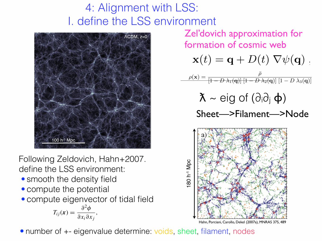
4: Alignment with LSS: I. define the LSS environment

ƛ ~ eig of (∂i∂j ɸ)

Following Zeldovich, Hahn+2007. define the LSS environment: • smooth the density field • compute the potential • compute eigenvector of tidal field

The Astrophysical Journal, 779:160 (10pp), 2013 December 20 Zhang et al.

survey boundary. For each group inside the volume coveringthe redshift range 0.01 ! z ! 0.12, the filling factor F is de-fined as the fraction of the survey volume in a sphere of radiusRF centered on this group. Generally, large F means that thegroup is located in the inner region of the survey volume, whilesmall F means that the group is near the boundary. Throughoutwe adopt RF = 80 h−1 Mpc, and we have tested that our re-sults are insensitive to changes in RF of a factor of two. We alsoemphasize that we have found the alignment signals to be insen-sitive to how we cull our sample based on F; using only groupswith F > 0.9 or all groups with F > 0 results in differencesin the average misalignment angles (see below for definition) of<0.◦1. Hence, in what follows we use all groups with F > 0.

2.2. Characterizing the Cosmic Web

In specifying the SDSS-MTV fields, Wang et al. (2012) usethe tidal tensor field

Tij (x) = ∂2φ

∂xi∂xj

, (1)

where i and j are indices with values of 1, 2, or 3, and φ is thepeculiar gravitational potential, which can be calculated fromthe distribution of dark matter halos with mass Mh above somethreshold value Mth through the Poisson equation,

∇2φ = 4 π G ρ δ = 4 π G ρ δh/bh . (2)

Here ρ is the average density of the universe, δ(x) = ρ(x)/ρ−1is the matter overdensity field, and δh(x) is the overdensity fieldof dark matter halos (groups) with mass Mh " Mth, whoseaverage linear bias parameter is given by bh. Thus, at the locationof each group we can derive φ and Tij using the distribution ofgroups with Mh " Mth (see Wang et al. 2012). Briefly, we firsttransform the redshift and sky coordinates for each group into aCartesian coordinate system using

X = R(z) cos δ cos α

Y = R(z) cos δ sin α (3)Z = R(z) sin δ,

where α and δ refer to the right ascension and declination,respectively, and R(z) is the comoving distance out to redshift z.Next, the halo overdensity field, δh, is computed on a rectangular(X, Y,Z) grid. This field is then corrected for redshift spacedistortions using the method of Wang et al. (2009a), which isbased on linear theory. Subsequently, fast Fourier transform isused to obtain the potential field, φ, by solving the Poissonequation (2), after which derivative operators are applied (inFourier space) to derive the tidal tensor.

This tidal tensor is subsequently diagonalized to obtain theeigenvalues λ1 " λ2 " λ3 of the tidal tensor at the position ofthe group, which, in analogy with Zel’dovich theory (Zeldovich1970), can be used to classify the group’s environment in oneof four classes:

1. cluster: a point where all three eigenvalues are positive;2. filament: a point where Tij has one negative and two

positive eigenvalues;3. sheet: a point where Tij has two negative and one positive

eigenvalues; and4. void: a point where all three eigenvalues are negative

Figure 1. Galaxy distributions and environmental classifications in a slice ofthickness 10 h−1 Mpc from SDSS DR7. The galaxy groups in four differentenvironments are classified by different colors: clusters (red), filaments (orange),sheets (green), voids (blue). The cyan arrow indicates the direction of thefilament at the center of each group. Black dots are groups with z > 0.12and therefore fall outside our survey volume, i.e., that have a filling factor F =0 (see text), and are therefore not included in the analysis.(A color version of this figure is available in the online journal.)

(see Hahn et al. 2007a, 2007b). Of the 277,139 galaxy groupswith Mh " Mth = 1012 h−1 M⊙ in our survey volume, 41,908groups (15.1%) are located in a cluster environment, 173,820groups (62.7%) are located in a filament, 57,169 groups(20.6%) are located in a sheet, and 4242 group (1.5%) arelocated in a void. Figure 1 shows the distribution of galaxygroups from the SDSS DR7 in a 200 h−1 Mpc × 200 h−1 Mpcslice of thickness 10 h−1 Mpc, in which groups in differentenvironment classes are indicated with different colors (see alsoWang et al. 2012).

2.3. Alignment Angles

The main goal of this study is to characterize to what extentthe orientation of galaxies is aligned with the structure of itssurrounding cosmic web (i.e., the orientation of filaments andsheets). To that extent we consider two alignment angles: forgalaxies whose group is located in a filament environment,we compute the angle θGF, defined as the angle between theorientation of the galaxy, θG, and the direction of the filament,θF. For galaxies whose group is located in a sheet environment,we instead compute the angle θGS, defined as the angle betweenθG and the normal direction of the sheet θS.

The orientation angle θG of the major axis of a galaxy,projected on the sky, is specified by the 25 mag arsec−1

isophote in the r band. The orientation angle of a filament,θF, at the location x of a filament group is computed asfollows. First, we identify the three-dimensional direction ∆xof the filament with the eigenvector corresponding to the singlenegative eigenvalue of the tidal tensor at x. Next, we computethe projected direction of the filament on the sky using

θF = arctan!

∆α cos δx

∆δ

", (4)

3

• number of +- eigenvalue determine: voids, sheet, filament, nodes

Galaxy Formation in the Cosmic Web Oliver Hahn Berkeley, Nov 18, 2008

180 h

-1 M

pc

Hahn, Porciani, Carollo, Dekel (2007a), MNRAS 375, 489

i. smooth density fieldii. compute potentialiii. compute eigenstructure

of tidal tensor

cluster

filamentsheet

void

(+++)

(++-)

(+--)

(---)

(as Zel’dovich approx. BUT on evolved non-linear field)

Tij � �i�j�

1

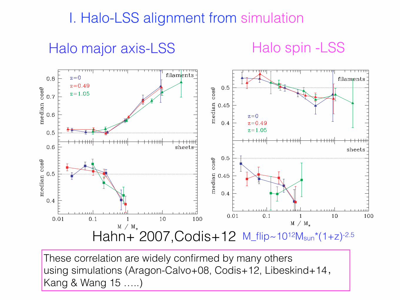
I. Halo-LSS alignment from simulation

Halo major axis-LSS Halo spin -LSS 48 O. Hahn et al.

80 90 100 110 120 130 140

30

40

50

60

70

80

90

h1

Mpc

h1

Mpc

Figure 8. Unit eigenvectors indicating the direction of the filaments are

shown in black for filament haloes in a slice of 8 h−1 Mpc in the 180 h−1 Mpc

box at z = 0. The grey symbols indicate halo positions regardless of their en-

vironment. The directional information of these vectors is used to determine

the alignment of halo spins with the LSS.

dynamical properties of the surrounding environment. Filaments

and sheets have a preferred direction given by the eigenvector cor-

responding the single positive or negative eigenvalue. The eigen-

vectors indicating the direction of the filament as determined from

the tidal tensor are shown in Fig. 8. Given these unit eigenvectors

v, we compute the alignment angle cos θ = J · v. Fig. 9 shows the

median alignment as a function of mass at redshifts z = 0, 0.49 and

1.05. At all redshifts, there is a strong tendency for sheet haloes to

have a spin vector preferentially parallel to the sheet, i.e. orthogonal

to the normal vector. At redshifts up to 0.49, where the error bars

of our measurements allow us to investigate trends with halo mass,

this alignment increases with increasing mass. For filament haloes,

there is a clear trend with halo mass: (i) haloes with masses smaller

than about 0.1M∗ have spins more likely aligned with the filament

in which they reside; (ii) haloes in the range M ≈ 0.1M∗ to 1M∗

appear to be randomly aligned with respect to the LSS and (iii) for

M ! M∗, the trend appears to reverse, and more massive haloes have

Figure 9. Median alignment angles between the halo angular momentum

vectors and the eigenvectors pointing in the direction of filaments and normal

to the sheets, respectively. Different redshifts are indicated with the three

colours. Error bars indicate the error in the median. The dotted line indicates

the expectation value for a random signal.

Figure 10. Median alignment angles between the halo major axis vectors

and the eigenvectors pointing in the direction of filaments and normal to the

sheets, respectively. Different redshifts are indicated with the three colours.

Error bars indicate the error in the median. The dotted line indicates the

expectation value for a random signal. Data are shown for the ratio of the

smoothing scale Ms/M∗ fixed.

a weak tendency to spin orthogonally to the direction of the filament

at lower redshifts.1

To further explore possible connections between the alignment

of the LSS and the intrinsic alignment of haloes in the different

environments, we search for a correlation signal between the LSS

and the axis vectors of the moment of inertia ellipsoid of the haloes.

In particular, we use the major axis vector l1 to define the alignment

angle cos θ = l1 · v, where v is again the eigenvector normal to a

sheet or parallel to a filament. The resulting median correlation is

shown in Fig. 10. We find no alignment for halo masses M < 0.1M∗;

however, in both the filaments and the sheets, the halo major axis

appears to be strongly aligned with the LSS for masses above about

a tenth of M∗. The strength of the alignment grows with increasing

mass. This is possibly to be expected, especially for the most massive

haloes, since their shape might influence the potential from which

the eigenvectors are derived. Adopting a fixed smoothing scale Ms

results merely in a shift of the relations shown in Fig. 10.

Results similar to ours concerning the alignments of shapes and

spins with the LSS, and the transition of alignment orientation at

M∗ in the filaments, are reported by Aragon-Calvo et al. (2007)

for z = 0 haloes using a definition of environment that is based on

density rather than, as in our case, on the gravitational potential,

as well as for haloes in the vicinity of clusters by Basilakos et al.

(2006) using the moment of inertia ellipsoid of superclusters and

by Ragone-Figueroa & Plionis (2007) defining environment by the

distance to the nearest cluster. It is clear from our present analysis

that such alignments are in place at redshifts of order one, and are

maintained virtually unchanged over the last eight or more billion

years of evolution of structure in the universe.

1 The tendency for haloes above M∗ to spin orthogonal to the host filament,

shown in Fig. 9 for the Ms/M∗ = const. smoothing case, is enhanced when the

Ms = const. smoothing is adopted. The smoothing scale not only determines

the environmental split of the halo population, but also affects the scale on

which the eigenvectors of the tidal field are computed. When the smoothing

is performed with Ms/M∗ = const., the filament direction is obtained on

increasingly smaller comoving scales at higher redshifts. This partially erases

the stronger correlation that is observed for the most massive haloes when

the smoothing is kept at constant comoving scale for all redshifts.

C⃝ 2007 The Authors. Journal compilation C⃝ 2007 RAS, MNRAS 381, 41–51

48 O. Hahn et al.

80 90 100 110 120 130 140

30

40

50

60

70

80

90

h1

Mpc

h1

Mpc

Figure 8. Unit eigenvectors indicating the direction of the filaments are

shown in black for filament haloes in a slice of 8 h−1 Mpc in the 180 h−1 Mpc

box at z = 0. The grey symbols indicate halo positions regardless of their en-

vironment. The directional information of these vectors is used to determine

the alignment of halo spins with the LSS.

dynamical properties of the surrounding environment. Filaments

and sheets have a preferred direction given by the eigenvector cor-

responding the single positive or negative eigenvalue. The eigen-

vectors indicating the direction of the filament as determined from

the tidal tensor are shown in Fig. 8. Given these unit eigenvectors

v, we compute the alignment angle cos θ = J · v. Fig. 9 shows the

median alignment as a function of mass at redshifts z = 0, 0.49 and

1.05. At all redshifts, there is a strong tendency for sheet haloes to

have a spin vector preferentially parallel to the sheet, i.e. orthogonal

to the normal vector. At redshifts up to 0.49, where the error bars

of our measurements allow us to investigate trends with halo mass,

this alignment increases with increasing mass. For filament haloes,

there is a clear trend with halo mass: (i) haloes with masses smaller

than about 0.1M∗ have spins more likely aligned with the filament

in which they reside; (ii) haloes in the range M ≈ 0.1M∗ to 1M∗

appear to be randomly aligned with respect to the LSS and (iii) for

M ! M∗, the trend appears to reverse, and more massive haloes have

Figure 9. Median alignment angles between the halo angular momentum

vectors and the eigenvectors pointing in the direction of filaments and normal

to the sheets, respectively. Different redshifts are indicated with the three

colours. Error bars indicate the error in the median. The dotted line indicates

the expectation value for a random signal.

Figure 10. Median alignment angles between the halo major axis vectors

and the eigenvectors pointing in the direction of filaments and normal to the

sheets, respectively. Different redshifts are indicated with the three colours.

Error bars indicate the error in the median. The dotted line indicates the

expectation value for a random signal. Data are shown for the ratio of the

smoothing scale Ms/M∗ fixed.

a weak tendency to spin orthogonally to the direction of the filament

at lower redshifts.1

To further explore possible connections between the alignment

of the LSS and the intrinsic alignment of haloes in the different

environments, we search for a correlation signal between the LSS

and the axis vectors of the moment of inertia ellipsoid of the haloes.

In particular, we use the major axis vector l1 to define the alignment

angle cos θ = l1 · v, where v is again the eigenvector normal to a

sheet or parallel to a filament. The resulting median correlation is

shown in Fig. 10. We find no alignment for halo masses M < 0.1M∗;

however, in both the filaments and the sheets, the halo major axis

appears to be strongly aligned with the LSS for masses above about

a tenth of M∗. The strength of the alignment grows with increasing

mass. This is possibly to be expected, especially for the most massive

haloes, since their shape might influence the potential from which

the eigenvectors are derived. Adopting a fixed smoothing scale Ms

results merely in a shift of the relations shown in Fig. 10.

Results similar to ours concerning the alignments of shapes and

spins with the LSS, and the transition of alignment orientation at

M∗ in the filaments, are reported by Aragon-Calvo et al. (2007)

for z = 0 haloes using a definition of environment that is based on

density rather than, as in our case, on the gravitational potential,

as well as for haloes in the vicinity of clusters by Basilakos et al.

(2006) using the moment of inertia ellipsoid of superclusters and

by Ragone-Figueroa & Plionis (2007) defining environment by the

distance to the nearest cluster. It is clear from our present analysis

that such alignments are in place at redshifts of order one, and are

maintained virtually unchanged over the last eight or more billion

years of evolution of structure in the universe.

1 The tendency for haloes above M∗ to spin orthogonal to the host filament,

shown in Fig. 9 for the Ms/M∗ = const. smoothing case, is enhanced when the

Ms = const. smoothing is adopted. The smoothing scale not only determines

the environmental split of the halo population, but also affects the scale on

which the eigenvectors of the tidal field are computed. When the smoothing

is performed with Ms/M∗ = const., the filament direction is obtained on

increasingly smaller comoving scales at higher redshifts. This partially erases

the stronger correlation that is observed for the most massive haloes when

the smoothing is kept at constant comoving scale for all redshifts.

C⃝ 2007 The Authors. Journal compilation C⃝ 2007 RAS, MNRAS 381, 41–51

Hahn+ 2007,Codis+12These correlation are widely confirmed by many others using simulations (Aragon-Calvo+08, Codis+12, Libeskind+14，Kang & Wang 15 …..)

M_flip~1012Msun*(1+z)-2.5

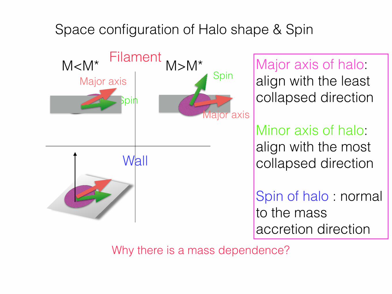
Space configuration of Halo shape & Spin

Major axis of halo: align with the least collapsed direction !Minor axis of halo: align with the most collapsed direction !Spin of halo : normal to the mass accretion direction

Why there is a mass dependence?

Spin

Major axisM<M* M>M*Filament

Wall

Spin

Major axis

II. Galaxy-LSS alignment from observationThe Astrophysical Journal, 779:160 (10pp), 2013 December 20 Zhang et al.

Figure 2. Normalized probability distribution of the angle θGF between theprojected orientation of the major axis of SDSS galaxies and that of the filamentin which its group resides. The horizontal dotted line corresponds to an isotropicdistribution of alignment angles, while the error bars indicate the scatter obtainedfrom 100 realizations in which the orientations of the galaxies have beenrandomized. The average value of θGF and its error (obtained from the 100random realizations) are indicated.

Figure 3. Same as Figure 2, but for the alignment angle θHF between theprojected orientation of a dark matter halo and that of the filament in which itresides. These results have been obtained using the numerical N-body simulationdescribed in Section 2.4.

axis of dark matter halos preferentially aligns parallel to thefilament in which it resides. The average alignment angle of⟨θHF⟩ = 43.◦30 ± 0.◦12 is smaller than for the SDSS galaxies.In addition, from N-body simulation we select a sample of darkmatter halos, with mass distribution equivalent to the host halosof central galaxies in the SDSS galaxy catalog. We find that thealignment signals for the dark matter halos are stronger thanthose of central galaxies in the SDSS galaxy catalog, and theaverage alignment angle is ⟨θHF⟩ = 42.◦19±0.◦38. This suggestsa net misalignment between the major axes of galaxies and theirdark matter halos, in excellent agreement with a number ofprevious alignment studies (e.g., Kang et al. 2007; Wang et al.2008; Okumura et al. 2009; Agustsson & Brainerd 2010; Liet al. 2013).

Figure 4. Same as Figure 2, but for different sub-samples (“red” and “blue“) ofcentral and satellite galaxies, as indicated.(A color version of this figure is available in the online journal.)

3.1.1. Dependence on Galaxy Properties

The large number (212,046) of filament galaxies in oursample allows us to study how the galaxy–filament alignmentsignal depends on various galaxy properties. We start by usingthe galaxy group catalog to split the galaxy population intocentrals (defined as the brightest group members) and satellites(those group members that are not centrals). These are furthersubdivided into “red” and “blue” according to their 0.1(g − r)colors: galaxies with 0.1(g − r) ! 0.83 are called “red,” whilethose with 0.1(g − r) < 0.83 are called “blue.” The value 0.83roughly corresponds to the bimodal scale in the color–magnituderelation (Weinmann et al. 2006).

Figure 4 shows the galaxy shape–filament alignment signalsfor the resulting four sub-samples. Central galaxies reveala remarkably strong color dependence. While red centralsshow strong alignment along their filaments, with ⟨θGF⟩ =43.◦26 ± 0.◦11, virtually identical to that of the dark matter halos(see Figure 3), blue filament centrals are only marginallyaligned, with an average misalignment angle that is consistentwith no alignment at the 2.3σ level. Satellite galaxies, overall,are less strongly aligned with the filaments in which their hostgroups reside than centrals. In particular, the orientations ofblue satellites are consistent at the 1.2σ level with having arandom (projected) orientation with respect to their filament.In the case of red satellites, however, the alignment signal is⟨θGF⟩ = 44.◦14 ± 0.◦19, which is significant at the 4.5σ level.

A quantitatively similar dependence on galaxy color has beenfound for the alignment between the orientation of centralgalaxies and the angular distribution of their satellites (Yanget al. 2006; Azzaro et al. 2007; Wang et al. 2008; Agustsson& Brainerd 2010) and suggests that red centrals are moreaccurately aligned with their host halo than blue centrals. Wecaution, though, that, as demonstrated by Kang et al. (2007),the interloper fraction (in the group catalog) is larger amongblue centrals than among red centrals, which may cause astronger dilution of the alignment signal for the blue centrals(since satellite galaxies show a weaker alignment signal). Wewill return to the interpretation of these findings in Section 4.

5

Galaxy Major axis-Filament4 Tempel & Libeskind

P(|

cos

θ|)

|cos(θ)|

e3-vector (filament axis)

<cos(θ)> = 0.513 <σ> = 1.62 pKS = 2.8⋅10-3

Spiral galaxies

0.8

1

1.2

0 0.2 0.4 0.6 0.8 1

P(|

cos

θ|)

|cos(θ)|

e2-vector

<cos(θ)> = 0.487 <σ> = 1.59 pKS = 3.4⋅10-3

Spiral galaxies

0.8

1

1.2

0 0.2 0.4 0.6 0.8 1

P(|

cos

θ|)

|cos(θ)|

e1-vector (sheet normal)

<cos(θ)> = 0.500 <σ> = 0.75 pKS = 6.3⋅10-1

Spiral galaxies

0.8

1

1.2

0 0.2 0.4 0.6 0.8 1

Figure 2. The orientation probability distribution between thespin axes of spiral galaxies and the filament/sheet orientation vec-tors. The panels and lines are the same as in Fig. 1.

ies are fed with mergers that occur along the filamentwithin which they are embedded. A similar mechanismhas been proposed for the formation of high-mass DMhalos (Codis et al. 2012).

4.2. Spiral galaxies

Figure 2 shows the correlation for spiral galaxies. Thelines and designations are the same as in Fig. 1. Figure 2shows that the spin axes of spiral galaxies tend to alignwith filaments (upper panel), which is consistent withprevious results (Tempel et al. 2013a). The middle panel

of Fig. 2, indicates that the spin axes of spirals are pref-erentially perpendicular to the e2-vector. The amount ofcorrelation is statistically the same as for the e3-vector.The lower panel of Fig. 2 shows that there is no statisti-cally significant correlation between the e1-vector (sheetnormal) and the spin axes of spiral galaxies. This impliesthat the formation of spiral galaxies is driven by the planeof the sheet along which most of the matter/gas falls into the filaments.Figure 3 shows the correlation between the spin of spi-

ral galaxies and e2, e3 as a function of distance to the fila-ment axis. Correlations are considerably stronger (basedon KS-test probabilities) for galaxies that are slightly fur-ther away (in the range 0.2–0.5h�1Mpc) than those thatare closer (0–0.2h�1Mpc) to the filament axis, which areconsistent with random. This implies that the correla-tions seen above are actually driven by those galaxiesslightly further way from the main filament axis. This isconsistent with the idea that the origin of the alignmentof angular momentum is related to the regions outside

Figure 3. The orientation probability distribution between thespin axes of spiral galaxies and the filament/sheet axes. Left (right)column shows the alignment signal for galaxies that are close to(slightly away from) the filament axis. Upper/lower panels showthe correlation for e3-/e2-vector.

filaments, namely sheets, where most of the gas is fallingin from. Along filament axes more chaotic motions dom-inate. Codis et al. (2012) also shows that the correlationbetween the rotation axes of DM halos and filaments isstronger in outer parts of filaments, supporting our find-ings.

5. DISCUSSION AND CONCLUSIONS

We have examined the alignment of spiral/ellipticalgalaxies with respect to the large-scale cosmic filamen-tary network. The correlation signal is calculated onlyfor bright galaxies that are located in filaments, wherewe also estimate the sheet orientation. The alignmentbetween galaxy spins and the axis of filaments/sheets ischaracterized by the shape of the probability distributionof cos ✓, where ✓ is the angle between the two vectors.A significant correlation between the short axes of el-

liptical galaxies and filament axes is found (the KS-testp-value is 7.7 · 10�9); these galaxies tend to be spin-ning perpendicular to the filament axis. For bright spiralgalaxies on the other hand the opposite is found: theytend to be aligned with the host filament axis. Both theseresults confirm earlier findings which employed di↵erentfilament finding algorithms (Tempel et al. 2013a).In this study, no alignment between the spin axes of

spiral galaxies in filaments and the e1-vector (sheet nor-mal) is found.A basic interpretation of filament formation suggests

that as a matter flows towards filaments, it wraps its up,thus aligning the filament axis with its angular momen-tum (as well as the vorticity of the filamentary matter,see Libeskind et al. 2013b). Spiral galaxies which con-dense out of filaments should thus preserve the perpen-dicular alignment between their spin and the direction ofmatter infall. If gas infall from sheets to filaments is lam-inar, it gives the parallel alignment between the spin axesof spiral galaxies and orientation of filaments. Assuming

Spin alignment in filaments and sheets 3

The quantity cos ✓ is obtained as a scalar product be-tween the two unit vectors: cos ✓ = 1 implies that thegalaxy spin is parallel to ei, while cos ✓ = 0 indicates itis perpendicular.The probability distribution function should be com-

pared with the null-hypothesis of random mutual orien-tation of galaxies and vectors. Due to selection e↵ects,this is not simply a uniform distribution; neither the in-clination angles of galaxies nor the distribution of fila-ment axes (with respect to the line-of-sight) have ran-dom orientations (see Tempel et al. 2013a). A Monte-Carlo approximation is used to estimate the distributionof | cos(✓)| for the case where there are no intrinsic corre-lations, and to find the confidence intervals for this esti-mate. This approach takes simultaneously into accountthe biases in filament detection (redshift-space distor-tions) and estimation of galaxy spins.In order to do so, 10000 randomized samples are gen-

erated in which the orientations (inclination and positionangles) of galaxies are kept fixed, but galaxy locations arerandomly changed between filament points. This givesthe true random orientation angle between the galaxyspin and filament axis. In principle, the randomized dis-tribution depends how the filament points are chosen:based on filament axes, location of galaxies etc. How-ever, for the current dataset it turns out to be insensi-tive to that. Using randomized samples the median ofthe null-hypothesis of a random alignment is calculatedtogether with its 95% confidence limits.The galaxy spin vector is not uniquely defined since we

do not know which side of the galaxy is closer to us. Inorder to handle this both spin vectors of a given galaxyare used. Varela et al. (2012) also tested this approachwith several Monte-Carlo simulations and showed thatthe procedure recovers correctly the probability distri-bution function.

4. RESULTS

4.1. Elliptical galaxies

Figure 1 shows the probability distribution P (| cos ✓|)for the angle ✓ between the short axes of elliptical galax-ies and the orientation vectors of filaments/sheets. Theprobability distribution is calculated for three principalvectors: e3, the filament axis; e1 the normal to the sheetwhere the filament is located and e2 – a vector perpen-dicular to these two. In each panel of Fig. 1 we alsoshow the average hcos(✓)i, the average deviation fromuniform distribution h�i (assuming a Gaussian distribu-tion where 95% confidence limit corresponds to ±2�) andthe Kolmogorov-Smirnov (KS) test probability pKS thatthe sample is drawn from a randomized distribution.The alignment between filament axes and the short

axes of elliptical galaxies is preferentially perpendicularas found previously (Tempel et al. 2013a). Note however,that the filament finding algorithm is di↵erent – Tempelet al. (2013a) used a locally defined morphological fil-tering, while here the object point process and globaloptimization is used. This shows that the result we ob-tained are rather robust and it does not depend on thefilament finding algorithm (for fixed filament scale).Moreover, estimating the short axes of elliptical galax-

ies is tricky since early type galaxies are triaxial ellipsoidsseen in projection. Due to the degeneracy between the

P(|

cos

θ|)

|cos(θ)|

e3-vector (filament axis)

<cos(θ)> = 0.479 <σ> = 3.38 pKS = 7.7⋅10-9

Elliptical galaxies

0.8

1

1.2

0 0.2 0.4 0.6 0.8 1

P(|

cos

θ|)

|cos(θ)|

e2-vector

<cos(θ)> = 0.510 <σ> = 1.72 pKS = 3.2⋅10-3

Elliptical galaxies

0.8

1

1.2

0 0.2 0.4 0.6 0.8 1

P(|

cos

θ|)

|cos(θ)|

e1-vector (sheet normal)

<cos(θ)> = 0.508 <σ> = 1.70 pKS = 1.1⋅10-2

Elliptical galaxies

0.8

1

1.2

0 0.2 0.4 0.6 0.8 1

Figure 1. The orientation probability distribution between theshort axes of elliptical galaxies and the filament/sheet axes. Up-

per panel shows the distribution for vectors parallel to filaments;middle panel shows the distribution for vectors perpendicular to fil-ament but parallel to the sheet; lower panel shows the distributionfor vectors perpendicular to the sheet where filament is located.The black line and the grey filled region show the null-hypothesistogether with its 95% confidence limit. The solid red line showsthe measured alignment signal.

intrinsic oblateness of the galaxy and the inclination an-gle, it is nearly impossible to properly estimate a spinaxis. The visible short axis of elliptical galaxies however,is easily observed, while the inclination angle is largelyundefined. Tempel et al. (2013a) showed that the corre-lation signal arises mostly from position angle of galaxiesand not from inclination angle. This implies that the truealignment signal is even stronger than what we are ableto measure.The middle and lower panel in Fig. 1 show the align-

ment signal between the short axes of elliptical galaxiesand the e2- and e1-vector, respectively. The correlationis practically the same for these two vectors. It showsthat the short axes of elliptical galaxies are preferentiallyperpendicular to filaments and the sheet orientation isnot important.Assuming that the short axis of an elliptical galaxy is

aligned with both its spin axis and the spin of the par-ent DM halo (however, there might be o↵set up to 30�,see e.g. Hahn et al. 2010), our findings allow us to com-ment on the formation mechanism of elliptical galaxies.It is known that elliptical galaxies formed predominantlythrough major mergers (e.g. Sales et al. 2012; Wilmanet al. 2013). In mergers, the rotation axis of the resultinggalaxy tends to be perpendicular to the merger direction.Our results are consistent with a picture wherein galax-

Spin - Filament

Zhang Y+2013 Tempel & Libeskind 2014

Observations agree well with Theory ! Signal is weaker (galaxy-halo misalignment)

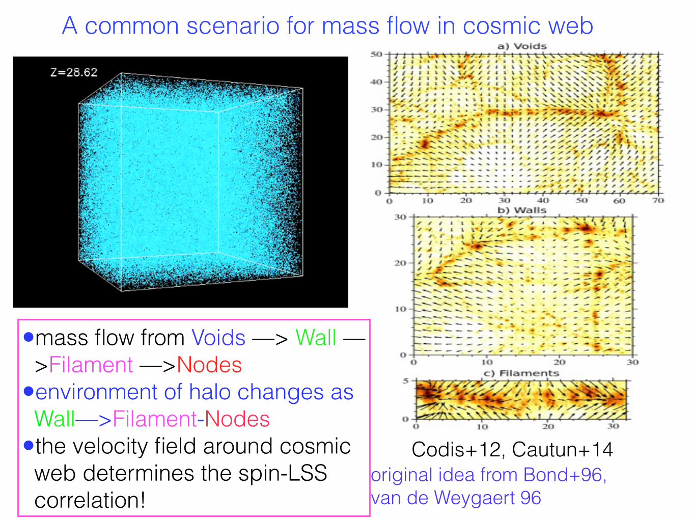
A common scenario for mass flow in cosmic web

Codis+12, Cautun+14

•mass flow from Voids —> Wall —>Filament —>Nodes

•environment of halo changes as Wall—>Filament-Nodes

•the velocity field around cosmic web determines the spin-LSS correlation!

original idea from Bond+96, van de Weygaert 96

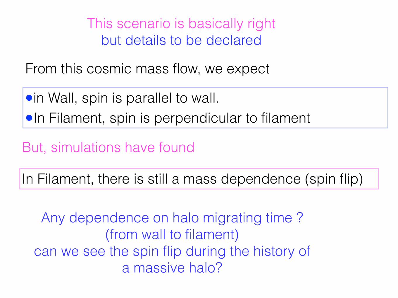
•in Wall, spin is parallel to wall. •In Filament, spin is perpendicular to filament

This scenario is basically right but details to be declared

From this cosmic mass flow, we expect

But, simulations have found

In Filament, there is still a mass dependence (spin flip)

Any dependence on halo migrating time ?(from wall to filament)

can we see the spin flip during the history of a massive halo?

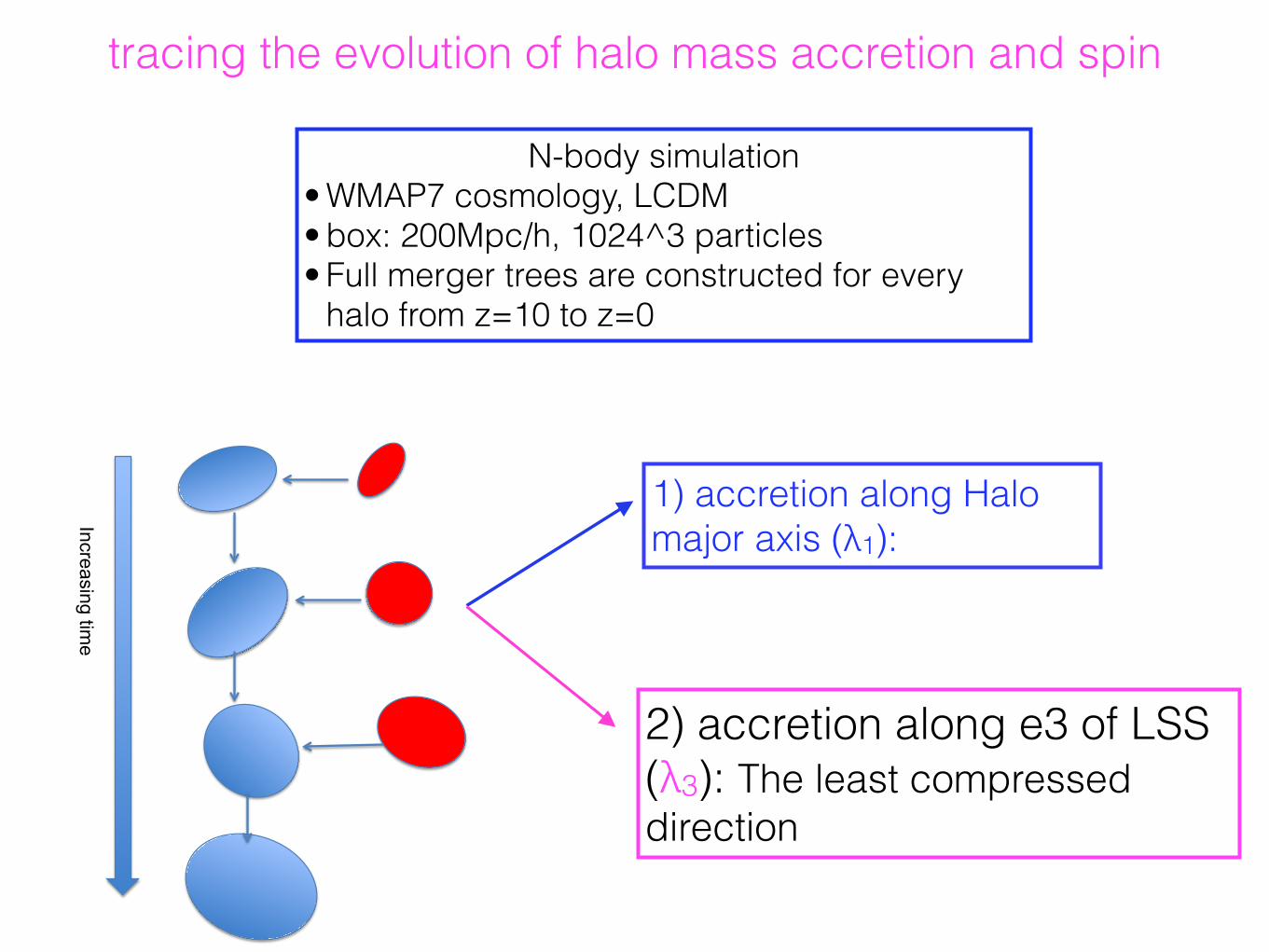
1) accretion along Halo major axis (λ1):

2) accretion along e3 of LSS (λ3): The least compressed direction

N-body simulation • WMAP7 cosmology, LCDM • box: 200Mpc/h, 1024^3 particles • Full merger trees are constructed for every

halo from z=10 to z=0

Increasing time

tracing the evolution of halo mass accretion and spin

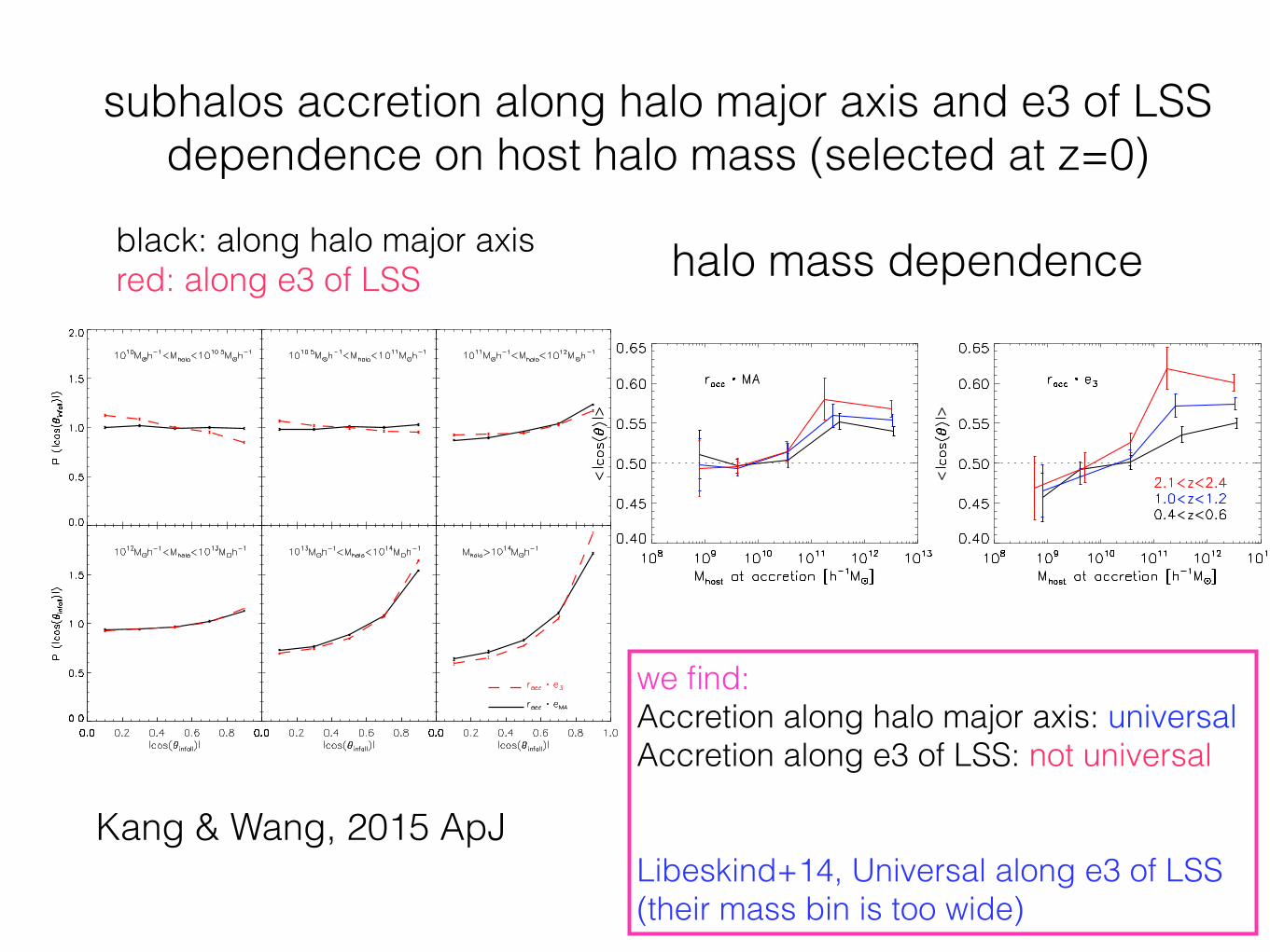
subhalos accretion along halo major axis and e3 of LSS dependence on host halo mass (selected at z=0)

– 13 –

Fig. 2.— The alignment of subhaloes with the halo major axis and e3 of LSS at their time of

infall (see text for detail). Different panels are for the final host halo at z = 0 with different mass.

The alignment with halo shape (black solid lines) is universal and increases with halo mass. The

alignment with e3 (red dashed lines) is stronger in massive haloes, but it is reversed for low-mass

haloes where it is perpendicular to e3.

black: along halo major axis red: along e3 of LSS

Kang & Wang, 2015 ApJ

– 15 –

Fig. 4.— The cumulative fraction of accreted mass in subhaloes with given alignment angle. Left

panel is for alignment with e3, and right for alignment with halo major axis. Higher fraction of

mass is accreted along e3 in massive haloes, and it becomes almost isotropic in low-mass haloes.

Fig. 5.— The alignment of subhaloes with host halo major axis (left panel) and the e3 direction of

LSS. Different from previous figures, here no constraints are posed on the final host halo mass, and

the accretion angles are binned depending on the accretion events with different host halo mass

and redshift. Seen is that accretion is always along the halo major axis (left panel). The alignment

with e3 is not universal and it is perpendicular to e3 for low-mass haloes, and the flip mass is lower

at high redshift (right panel).

we find: Accretion along halo major axis: universal Accretion along e3 of LSS: not universal !!Libeskind+14, Universal along e3 of LSS (their mass bin is too wide)

halo mass dependence

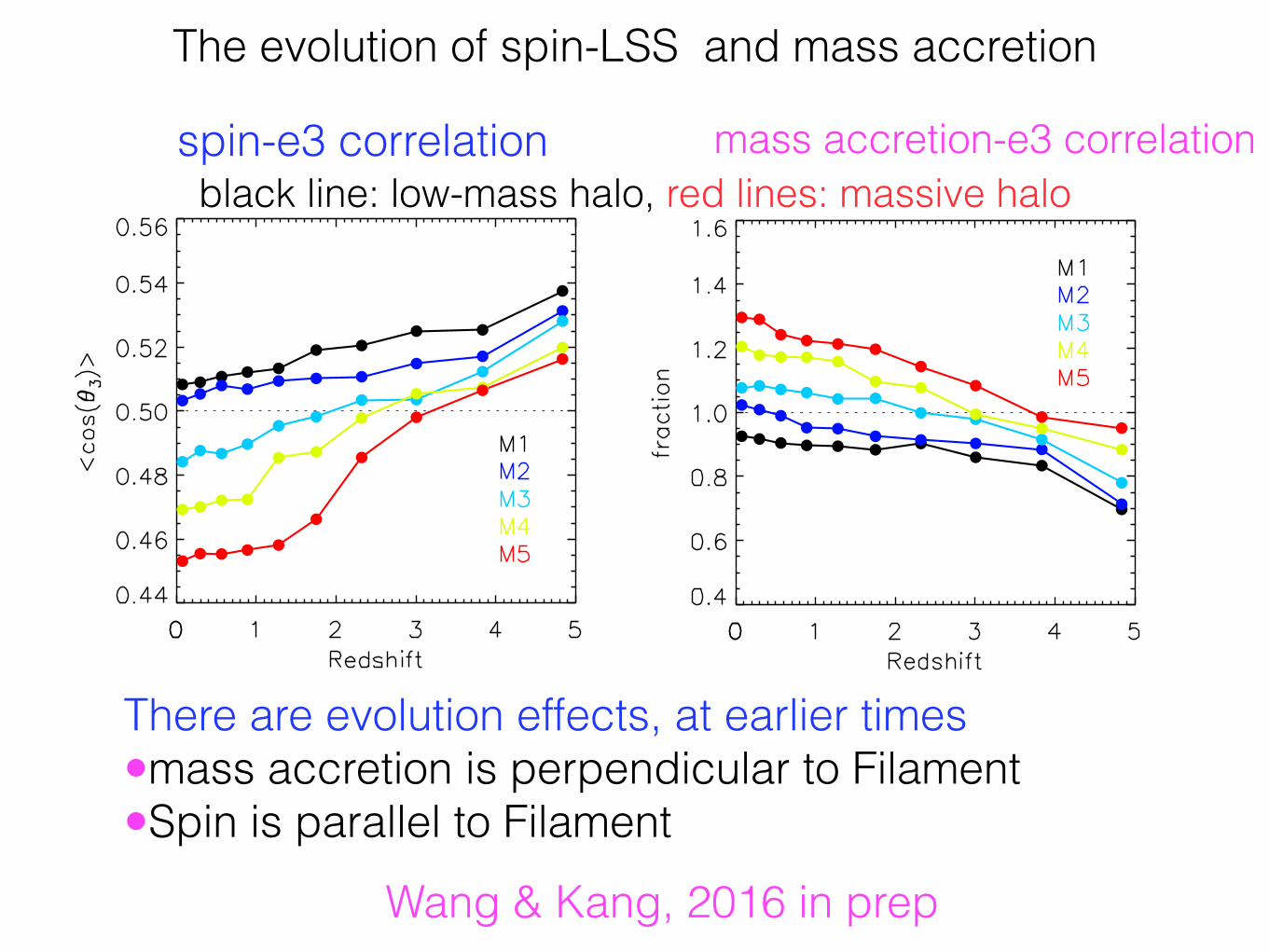
The evolution of spin-LSS and mass accretion

– 2 –

Fig. 3.— Right: the average cosine of angle ✓3 between halo spin and e3 direction as a function of

halo mass and redshift. Left: same as the right panel, but halo mass is normalized by M?.

Fig. 4.— The evolution of average cos✓3, ✓3 is the angle between halo spin and the e3 direction.

The value 0.5 represents the random distribution of spin to e3. Mass increase from M1 to M5,

10

10M� ⇠ 10

11M� for M1, 10

11M� ⇠ 10

12M� for M2, 10

12M� ⇠ 10

12.5M� for M3, 10

12.5M� ⇠

10

13M� for M4, M5 represents halo mass > 10

13M�. Smooth length is 2Mpc at z = 0 and it

evolves by redshift: 2Mpc/(1+z).

– 3 –

Fig. 5.— The fraction f as a function of redshift. f is the fraction of mean mass of subhaloes be

accreted along the filament over mean mass of subhaloes be accreted perpendicular to filament.

f = 1 means host haloes accrete subhaloes randomly. f > 1 represents host haloes accrete subhaloes

along the filament direction. Same as Fig. 4, from M1 to M5 represents di↵erents halo mass bin.

In the lower right panel we find that low-mass haloes accrete subhaloes perpendicular to filament

all the time, but for massive haloes, they eat subhaloes perpendicular to filament at high redshift,

then at low redshifit, subhaloes be accreted to these massive haloes along filament. This result

agrees with our last work and this may explain the spin flips during time in Fig. 4.

spin-e3 correlation mass accretion-e3 correlation

There are evolution effects, at earlier times •mass accretion is perpendicular to Filament •Spin is parallel to Filament

Wang & Kang, 2016 in prep

black line: low-mass halo, red lines: massive halo

An useful parameter for anisotropic collapse

The velocity shear tensor 2493

The distribution of eigenvalues for those regions of space thatcontain haloes (black, blue and red curves in Fig. 2) shows a numberof interesting attributes as well. Despite all being drawn from thesame parent distribution (green curves), they are qualitatively verydifferent. First, we note that none of the eigenvalue distributions(when binned by mass) resemble the parent distribution in terms ofwidth or median. The low-mass bin (black curve) peaks at a similarvalue to the parent distribution, probably owing to the fact that thismass bin spans the largest fraction of grid cells. Yet, the peak of eachdistribution is clearly mass dependent. The more massive the set ofhaloes being examined, the greater the median of the distribution.Intuitively, this is because the most massive haloes reside in regionsof strong gravitational collapse that is, regions with larger valuesof λ.

3.1 The fractional anisotropy: the distribution of shearsphericity

The semi-infinite range of eigenvalues (described above) makes itdifficult to characterize the uniformity of the collapse or expansionin the way that, for example, the inertia tensor may be characterizedby its triaxiality. In their seminal work on Gaussian random fields,Bardeen et al. (1986) defined the ‘eccentricity’ e of a density field(not a shear) as

e = λ1 − λ3

2|δ|, (5)

where in the linear regime the dimensionless overdensity is definedas the trace of the shear, i.e. equation (3). This measure of eccen-tricity has been used by a number of authors (e.g. Lee & Lee 2008)when examining velocity shears. That said, the original Bardeenet al. definition was invoked in a system with three positive eigen-values (such as the inertia tensor) and not in the situation where theeigenvalues are bound by (− ∞, ∞) as in the shear tensor.

The usage of the Bardeen et al. eccentricity is therefore highlyproblematic in our situation. In cases where λ1 ∼ −λ3, small valuesof λ2 can cause the denominator of equation (5) to tend to 0 makinge highly unstable. Also, the fact that e is semi-infinite makes it moredifficult to compare vastly different eccentricities.

In order to overcome these difficulties, the amount of anisotropyin the shear tensor can be characterized using the fractionalanisotropy, FA,

FA = 1√3

!(λ1 − λ3)2 + (λ2 − λ3)2 + (λ1 − λ2)2

λ21 + λ2

2 + λ23

, (6)

which measures the fraction of the magnitude of the shear thatis due to the anisotropy of the eigenvalues (Basser 1995).2 Notethat 1/

√3 is introduced to normalize the fraction to unity. This

definition is employed to characterize the uniformity of the collapseor expansion.

The FA measures the kinematical ‘morphology’ of the velocityshear. It is superior to the eccentricity since it is forced to be betweenzero and unity. FA = 0 implies isotropic expansion or collapsein all three directions. In filaments and sheet volumes, FA = 1

2 The concept of the Fractional Anisotropy was developed in the field of Nu-clear Magnetic Resonance by Basser (1995) as a tool in brain imaging. Thediffusivity of water molecules through cerebral tissue, one of the quantitiesmeasured by an NMR scan, constitutes an identical process to the velocityshear. Thus both the cosmic velocity shear tensor and the diffusion tensor inbrain scans can be quantified by the Fractional Anisotropy.

Figure 3. The fractional anisotropy FA is a measure of shear anisotropy.Since each halo can be assigned a web type based on the local velocity shearcalculated at its location, we divide our halo sample into four web classes,plotting the probability density distribution of FA for haloes resident in knots(black), filaments (green), sheets (blue) and voids (red). Each distributionis normalized by the number of objects in it. FA = 0 indicates uniformexpansion or collapse. Since the peaks and widths of these distributionsdepend on web type, we infer that each web type behaves differently: knotcollapse is not simply void expansion played in reverse.

indicates that collapse along e1 is of roughly the same strength asexpansion along e3, while in knots and voids, FA = 1 indicates largeanisotropies in the expansion or contraction.

In Fig. 3 we show the distribution of the local velocity shearFA. Since each web type represents a different number of positiveeigenvalues, we plot them separately. A number of important pointscan be gleaned from this figure.

(i) The collapse in knot environments is relatively isotropic; thatis, the value of FA measured in knots tends to be low. The strength ofthe velocity shear in knot environments thus displays a remarkableregularity.

(ii) The distribution of FA in filaments and sheets is wide – theshear that defines these web types takes on a myriad of kinematicalmorphologies. Whereas filaments peak at lower values of FA, sheetspeak at higher values.

(iii) Void regions have high values of FA indicating highlyanisotropic expansion.

We thus conclude from Fig. 3 that the cosmic web reflects a re-markable variety of shear anisotropies. Voids, for example, are oftennot kinematically isotropic objects. Knots display significantly moreuniformity than voids, and also span a wide range of sphericities.Filaments and sheets, on the other hand, while displaying some sim-ilarities are still coloured by a variety of corpulence: some filamentsare fat, some are thin, some sheets are thick, some are narrow.

The FA is shown graphically in Fig. 4. Since voids dominate thevolume, the figure emphasizes the rich diversity in the kinematic‘morphology’ of voids. Although it appears that much of the voidvolume is represented by regions of high FA (white areas in Fig. 4),

at Nanjing U

niversity on Decem

ber 28, 2015http://m

nras.oxfordjournals.org/D

ownloaded from

Large FA: highly anisotropy Lower FA: collapse happen on all directionsƛ ~ eig of (∂i∂j ɸ)

– 4 –

Fig. 6.— Right: the cos✓3 as a function of FA for all haloes, here smooth length is 4,8,16 times of

Rvir in each mass bin. Left: the FA as a function of halo mass; filament and cluster environment;

redshift with smooth length 4Rvir.

Fig. 7.— Same as Fig. 6, but show two di↵erent mass haloes to see the mass dependence.

– 4 –

Fig. 6.— Right: the cos✓3 as a function of FA for all haloes, here smooth length is 4,8,16 times of

Rvir in each mass bin. Left: the FA as a function of halo mass; filament and cluster environment;

redshift with smooth length 4Rvir.

Fig. 7.— Same as Fig. 6, but show two di↵erent mass haloes to see the mass dependence.

Wang & Kang, 2016 in prep Nodes: spin is normal to e3 Filament: mass dependence

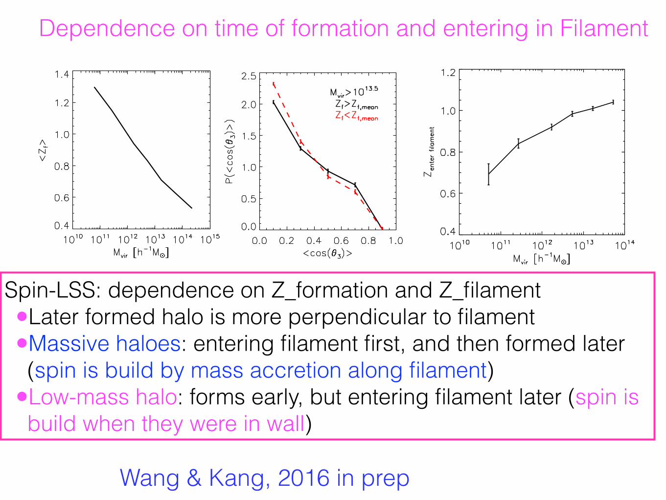
Dependence on time of formation and entering in Filament– 5 –

Fig. 8.— Left: the formation time of halo as a function of halo mass. low-mass halo form earlier

than high-mass halo. Right: spin-lss correlation as a function of halo formation time.

Fig. 9.— The redshift Zenterfilament as a function of halo mass, which Zenterfilament is the redshift

of halo environment change from sheet to filament and halo mass is the mass at z = 0.

– 5 –

Fig. 8.— Left: the formation time of halo as a function of halo mass. low-mass halo form earlier

than high-mass halo. Right: spin-lss correlation as a function of halo formation time.

Fig. 9.— The redshift Zenterfilament as a function of halo mass, which Zenterfilament is the redshift

of halo environment change from sheet to filament and halo mass is the mass at z = 0.

– 5 –

Fig. 8.— Left: the formation time of halo as a function of halo mass. low-mass halo form earlier

than high-mass halo. Right: spin-lss correlation as a function of halo formation time.

Fig. 9.— The redshift Zenterfilament as a function of halo mass, which Zenterfilament is the redshift

of halo environment change from sheet to filament and halo mass is the mass at z = 0.

Spin-LSS: dependence on Z_formation and Z_filament •Later formed halo is more perpendicular to filament •Massive haloes: entering filament first, and then formed later (spin is build by mass accretion along filament)

•Low-mass halo: forms early, but entering filament later (spin is build when they were in wall)

Wang & Kang, 2016 in prep

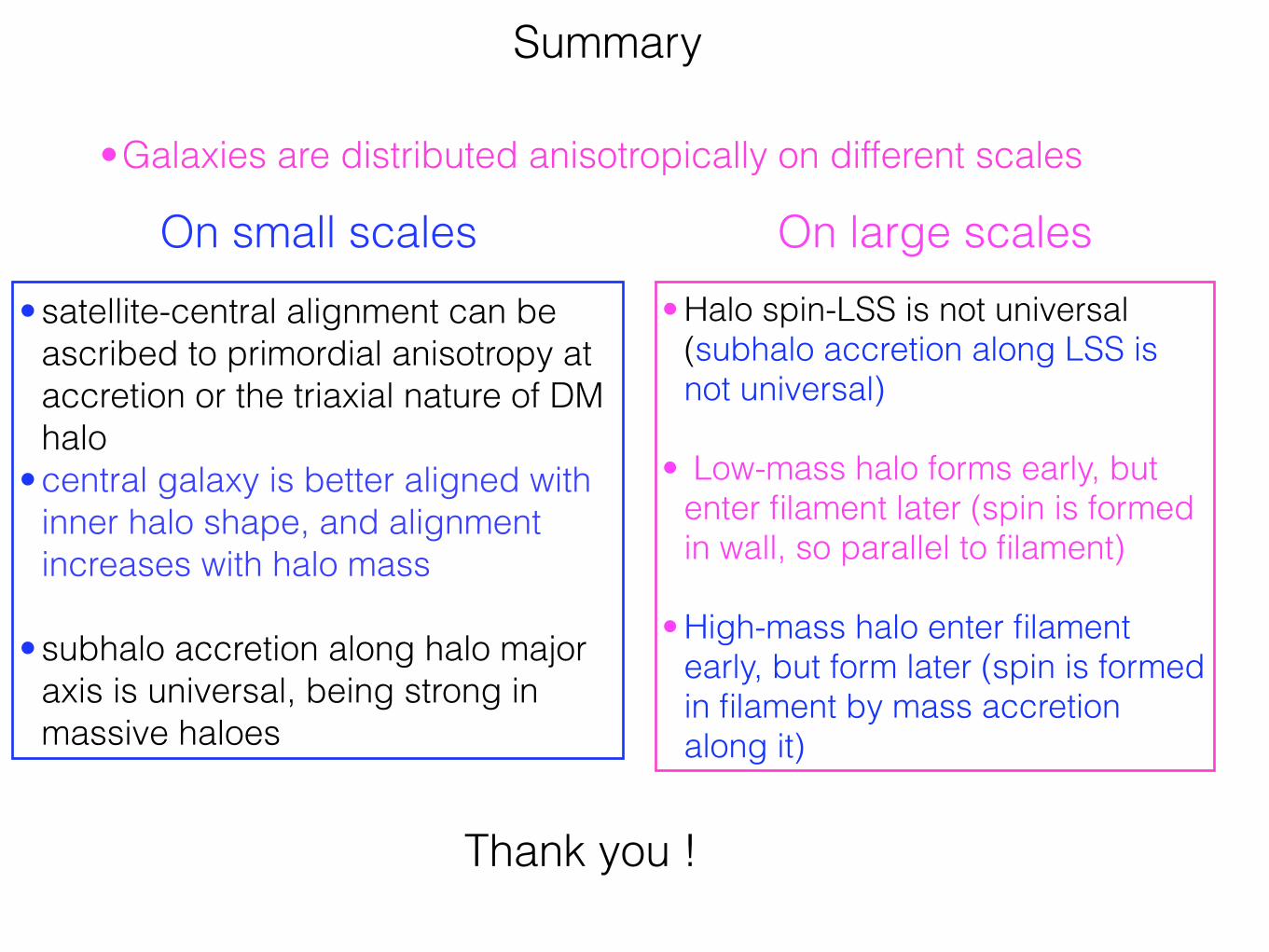
• satellite-central alignment can be ascribed to primordial anisotropy at accretion or the triaxial nature of DM halo

• central galaxy is better aligned with inner halo shape, and alignment increases with halo mass !

• subhalo accretion along halo major axis is universal, being strong in massive haloes

• Halo spin-LSS is not universal (subhalo accretion along LSS is not universal)

!• Low-mass halo forms early, but

enter filament later (spin is formed in wall, so parallel to filament)

!• High-mass halo enter filament

early, but form later (spin is formed in filament by mass accretion along it)

Summary

•Galaxies are distributed anisotropically on different scales

On small scales On large scales

Thank you !