Embed Size (px)
Citation preview

1 of 113
GAME THEORY ANALYSIS OF AIRCRAFT MANUFACTURER INNOVATION STRATEGIES
IN THE FACE OF INCREASING AIRLINE FUEL COSTS
James K.D. Morrison, Sgouris Sgouridis and R. John Hansman
This report is based on the Master Thesis of James K.D. Morrison submitted to the Engineering Systems Division in partial fulfillment of the requirements for the degree of
Master of Science in Technology and Policy at the Massachusetts Institute of Technology.
Report No. ICAT-2011-4 June 2011
MIT International Center for Air Transportation (ICAT)
Department of Aeronautics & Astronautics Massachusetts Institute of Technology
Cambridge, MA 02139 USA

2 of 113
[Page Intentionally Left Blank]

3 of 113
Game Theory Analysis of Aircraft Manufacturer Innovation Strategies in the Face of Increasing Airline Fuel Costs
by
James K.D. Morrison, Sgouris Sgouridis, and R. John Hansman
Abstract
The air transportation system is a vital infrastructure that enables economic growth and provides significant social benefits. Future increases and volatility in crude oil prices, as well as environmental charges, are likely to increase the effective cost of fuel. We investigate the impacts of effective fuel cost increase on the US air transportation system historically and perform a game theory analysis of the impact of manufacturer competition on the introduction of new, more fuel efficient aircraft.
The cost of jet fuel increased 244% between July 2004 and July 2008, providing a natural experiment to evaluate how fuel price increase affected continental US networks and fleets. It was found that non-hub airports serving small communities lost 12% of connections, compared to a system-wide average loss of 2.8%. Increased effective fuel costs will provide incentives for airlines to improve fleet fuel efficiency, reducing the environmental impacts of aviation, but may cause an uneven distribution of social and economic impacts if small communities suffer greater loss of mobility. Government action may be required to determine acceptable levels of access as the system transitions to higher fuel costs.
Technology innovation may act as a long-term hedge against increasing effective fuel costs, enabling mobility to be maintained. The single aisle commercial aircraft market segment is the largest, but has the longest running product lines. We hypothesize that competition has important effects on manufacturers’ decisions to innovate that must be considered when designing policies to reduce fleet emissions. An aircraft program valuation model is developed to estimate expected payoffs to manufacturers under competitive scenarios. A game theory analysis demonstrates how the incentives to innovate may be altered by subsidies, technology forcing regulations, increased effective fuel costs, the threat of new entrants, and long-term competitive strategies. Increased competition may result in incumbent manufacturers producing re-engined aircraft while increased effective fuel costs may result in new aircraft programs. Incumbents’ optimal strategies may be to delay the entry of new single aisle aircraft until 2020-24, unless technology forcing regulations are implemented.

4 of 113
Acknowledgements
This work was supported by the MIT/Masdar Institute of Science and Technology
under grant number Mubadala Development Co. Agreement 12/1/06. The authors wish to
thank PARTNER for access to the Piano-X software package and Robert M. Peterson
from the Boeing Corporation for his valuable feedback on the aircraft program valuation
model. Any errors are the authors’ alone.

5 of 113
Table of Contents
Abstract.............................................................................................................................. 3
Acknowledgements ........................................................................................................... 4
Table of Contents .............................................................................................................. 5
List of Figures.................................................................................................................... 7
List of Tables ..................................................................................................................... 9
Acronyms and Abbreviations ........................................................................................ 10
1.0 Introduction............................................................................................................... 11
1.1 Motivation........................................................................................................................11 1.2 Macroeconomic Model of the Air Transportation System ..............................................12 1.3 Reducing Commercial Aviation’s CO2 Emissions ..........................................................13 1.4 Thesis Outline ..................................................................................................................15
2.0 Research Approach................................................................................................... 16
2.1 Research Questions..........................................................................................................16 2.2 Research Approach ..........................................................................................................17
3.0 Impacts of Effective Fuel Cost Increase.................................................................. 22
3.1 Historical Case Study: 2004-08 Fuel Price Surge ...........................................................23 3.2 Potential Factors Influencing Airline and Passenger Decisions ......................................33 3.3 Extrapolating Findings to Future Scenarios.....................................................................39 3.4 Policies to Reduce Social and Economic Impacts ...........................................................43 3.5 Summary..........................................................................................................................45
4.0 Improving Fleet Fuel Efficiency Through Technology Innovation...................... 47
4.1 Historical Aircraft Fuel Intensity Improvements.............................................................47 4.2 Future Potential Fuel Intensity Improvements.................................................................53 4.3 Economics and Dynamics of Implementation of Mitigating Measures ..........................57 4.4 Single Aisle Aircraft Market Structure ............................................................................58 4.5 Structure of the Competitive Game .................................................................................63

6 of 113
4.6 Summary..........................................................................................................................65
5.0 Methodology for Aircraft Program Valuation....................................................... 67
5.1 Making the Case for New Aircraft Programs ..................................................................68 5.2 Aircraft Program Valuation Model..................................................................................69 5.3 Sensitivity Analysis .........................................................................................................84 5.4 Summary..........................................................................................................................85
6.0 Game Theory Analysis of the Incentives to Innovate ............................................ 86
6.1 Game Theory ...................................................................................................................86 6.2 Two-Player Static Games ................................................................................................89 6.3 Three-Player Static Games ..............................................................................................94 6.4 Two-Player Dynamic Game ............................................................................................97 6.5 Three-Player Dynamic Games.........................................................................................99 6.6 Summary........................................................................................................................101
7.0 Conclusions.............................................................................................................. 103
8.0 References................................................................................................................ 106
9.0 Appendix: Airline Classification ........................................................................... 113

7 of 113
List of Figures
Figure 1. Correlation Between GDP and Passenger Traffic in the US............................. 11
Figure 2. Air Transportation System and Effective Fuel Cost Macroeconomic Interaction
Model............................................................................................................. 13
Figure 3. Cumulative Potential Reductions in CO2 Emissions from 2006 to 2050.......... 14
Figure 4. Trends in Crude Oil and Jet Fuel Prices During the Time Periods of Study..... 23
Figure 5. Trends in US Airline Industry Unit Operating Costs. ....................................... 24
Figure 10. Airline Network Configurations...................................................................... 28
Figure 11. Continental US Air Transportation Network Freeman Index, 2004-08 .......... 29
Figure 12. Continental US Airline Network Freeman Indices, 2004-08 .......................... 29
Figure 13. Next Nearest Airport with Passenger Departures to Airports that Lost All
Service, July 2007-08 .................................................................................... 30
Figure 14. Continental US Access to Airports with Regular Service............................... 31
Figure 15. Aircraft Type 2006 Operating Fuel Intensity .................................................. 35
Figure 16. Change in Revenue Miles Flown by Aircraft Type Fuel Intensity ................. 35
Figure 17. Cost and Revenue per ASM - Q3 2007 and 2008 Comparison....................... 37
Figure 18. Price Elasticities of Demand for Air Transportation....................................... 38
Figure 19. Jet Fuel Price Forecast..................................................................................... 40
Figure 20. US Passenger Carrier Domestic Operational Fuel Intensity, 2000-2009 ........ 41
Figure 21. EAS Subsidies and Continental US Communities Served by EAS ................ 44
Figure 22. Trend in Transport Aircraft Fuel Efficiency ................................................... 49
Figure 23. Reduction in Fuel Consumption and CO2 Emissions by Engine Technology 49
Figure 24. Future Aircraft Energy Usage ......................................................................... 50
Figure 25. Energy Intensity of Regional Aircraft Compared to Fleet Averages .............. 51
Figure 26. Aircraft Fuel Efficiency Trends and Projections............................................. 52
Figure 27. Sales-Weighted Average Jet Aircraft Fuel Burn, 1960-2008.......................... 53
Figure 28. Life Cycles and Replacement of Jet Aircraft Class Product ........................... 53
Figure 29. Distribution of Mitigating Measures’ Start and Diffusion Times ................... 56
Figure 30. CO2 Marginal Abatement Cost Curve for the 2012 European Fleet ............... 57

8 of 113
Figure 31. Large Commercial Aircraft Manufacturer Market Shares by Deliveries ........ 59
Figure 32. Narrow Body Single-Aisle Jet Aircraft, 1980-2010........................................ 60
Figure 33. Single Aisle, 150-185 Seat Market Shares and Fuel burn Performance, 1980-
2009 ............................................................................................................... 61
Figure 34. The Productive Pyramid in the Civil Aeronautic Industry.............................. 62
Figure 35. Potential Fuel Burn Improvements of Future Technologies ........................... 64
Figure 36. Structure of the Static and Dynamic Games Analyzed ................................... 65
Figure 37. Narrow Body Deliveries, 1990-2009 .............................................................. 71
Figure 38. Annual Percent Change in 737 and A320 Deliveries, 1990-2009................... 72
Figure 39. The Benefits of Advanced Technology – Fuel Related Cost Savings............. 74
Figure 40. A320/737-800 Lifecycle Cost Estimates......................................................... 75
Figure 41. Estimation of Average Aircraft List Price Discounts for All Deliveries......... 76
Figure 42. Cost Analysis Approach to Price Setting ........................................................ 77
Figure 43. Wide Body, Medium Range Market Share Analysis. ..................................... 78
Figure 44. Wide Body, Long Range Market Share Analysis. .......................................... 79
Figure 45. Aircraft Program Valuation Cumulative Distribution Functions for Symmetric
Strategies........................................................................................................ 83
Figure 46. Sensitivity of New Aircraft Program E(NPV) to Changes in Input
Assumptions. ................................................................................................. 84
Figure 47. Game 1 Expectation of Low Fuel Prices Decision Timeline .......................... 89
Figure 48. Game 2 Technology Forcing Regulations Decision Timeline ........................ 90
Figure 49. Game 3 Manufacturer Subsidies Decision Timeline....................................... 91
Figure 50. Game 4 Expectation of Increasing Fuel Prices Decision Timeline................. 93
Figure 51. New Entrant Extended Form Game ................................................................ 94
Figure 52. Game 5 New Entrant, -25% Fuel Intensity Decision Timeline....................... 95
Figure 53. Game 6 New Entrant, -15% Fuel Intensity Decision Timeline....................... 96
Figure 54. Game 7 Two-Player Dynamic Game Decision Timeline................................ 97
Figure 55. Game 8 New Entrant Dynamic Game, -25% Fuel Intensity Decision Timeline
....................................................................................................................... 99
Figure 56. Game 9 New Entrant Dynamic Game, -15% Fuel Intensity Decision Timeline
..................................................................................................................... 100

9 of 113
List of Tables
Table 1. Number of Airports by Class with Continental US Passenger Departures......... 28
Table 2. Changes in Continental US Passenger Departures, July 2007-08 ...................... 28
Table 3. The Airline Network Configuration Matrix........................................................ 27
Table 4. Annualized Changes in US Carrier Domestic Supply and Demand................... 32
Table 5. Annualized Changes in US Carrier International Supply and Demand.............. 33
Table 6. NASA’s Environmentally Responsible Aviation (ERA) Project Goals for
Subsonic Vehicles.......................................................................................... 55
Table 7. Selection of Technologies to Improve Fuel Efficiency. ..................................... 56
Table 8. Base Case Aircraft Demand Binomial Lattice Model ........................................ 73
Table 9. Base Case Jet Fuel Price Binomial Lattice Model.............................................. 74
Table 10. Aircraft Lifecycle Fuel Cost Model Input Parameters...................................... 75
Table 11. Two Player Game Market Share Rules............................................................. 80
Table 12. Three Player Game Market Share Rules........................................................... 80
Table 13. Three Player Game Market Share Rules........................................................... 80
Table 14. Aircraft Program Valuation Model Assumptions............................................. 82
Table 15. Valuation Model Symmetric Strategy Statistics............................................... 83
Table 16. Overview of Games Played .............................................................................. 89
Table 17. Game 1 Low Fuel Prices................................................................................... 90
Table 18. Game 2 Technology Forcing Regulations ........................................................ 91
Table 19. Game 3 Manufacturer Subsidies....................................................................... 92
Table 20. Game 4 Increasing Fuel Prices ......................................................................... 93
Table 21. Game 5 New Entrant, -25% Fuel Intensity....................................................... 96
Table 22. Game 6 New Entrant, -15% Fuel Intensity....................................................... 96
Table 23. Game 7 Two-Player Dynamic Game................................................................ 98
Table 24. Game 8 New Entrant 2015 Dynamic Game, -25% Fuel Intensity.................. 100
Table 25. Game 9 New Entrant 2015 Dynamic Game, -15% Fuel Intensity.................. 101
Table 26. Summary of Game Equilibriums .................................................................... 102

10 of 113
Acronyms and Abbreviations
Acronyms Description ASM : Available Seat Mile ASK : Available Seat Kilometre ATA : Air Transport Association BEA : Bureau of Economic Analysis (United States) BTS : Bureau of Transportation Statistics (United States) CASM : Cost per Available Seat Mile CDF : Cumulative Distribution Function CO2 : Carbon Dioxide DOT : Department of Transportation (United States) EAS : Essential Air Service (United States DOT Program) EIA : Energy Information Administration (United States) E(NPV) : Expected Net Present Value EPA : Environmental Protection Agency (United States) ERA : Environmentally Responsible Aviation (NASA Project) EU ETS : European Union Emissions Trading Scheme FAA : Federal Aviation Administration GAO : Government Accountability Office (United States) GDP : Gross Domestic Product GHG : Green House Gas(es) GTF : Geared turbofan (Engine) HHI : Herfindahl-Hirschman Index IATA : International Air Transport Association ICAO : International Civil Aviation Organization (United Nations) IPCC : Intergovernmental Panel on Climate Change (United Nations) IRR : Internal Rate of Return LCC : Low Cost Carrier MAC : Marginal Abatement Cost MDO : Multidisciplinary Design Optimization NASA : National Aeronautics and Space Administration (United States) NLC : Network Legacy Carrier NPV : Net Present Value NTSB : National Transportation Safety Board (United States) OEW : Operational Empty Weight RASM : Revenue per Available Seat Mile RDT&E : Research, Development, Testing, and Evaluation RPM : Revenue Passenger Mile TAROC : Total Aircraft Related Operating Cost TFUC : Theoretical First Unit Cost WACC : Weighted Average Cost of Capital

11 of 113
CHAPTER 1
1.0 Introduction
1.1 Motivation
The air transportation system is a vital infrastructure that enables economic
growth and provides significant social benefits. To access larger markets, businesses
locate near airports. Families pursue global career and leisure opportunities that are only
enabled by aviation. Hospitals require time sensitive diagnostic materials transported by
air. There is a correlation between GDP and passenger traffic growth, as shown in Figure
1:
Figure 1. Correlation Between GDP and Passenger Traffic in the US. Data Source: BTS, 2009; Bureau of Economic Analysis, 2009; National Bureau of Economic Research, 2009. Courtesy of Dr. P. Bonnefoy. As developing economies grow, the demand for air transportation will increase.
Passenger traffic is expected to continue to grow at a rate of 4-6% annually while jet
aircraft fuel efficiency has historically improved at a rate of 1.2-2.2% per year on a seat-
km basis. Fuel efficiency improvements have not been sufficient to counter increased
emissions due to rising demand for air transport (Lee et. al., 2001).

12 of 113
Future increases and volatility in crude oil prices, as well as environmental
charges (e.g. CO2 cap and trade, carbon taxes), are likely to increase the effective cost of
fuel. As the supply of crude oil tightens, without significant reductions in worldwide
demand, prices will increase. Geopolitical events and acts of nature may result in price
surges that shock industries reliant on fossil fuel energy sources. Further, as climate
change concerns mount, governments will face increasing pressure to take action to
reduce the emission of carbon dioxide and other greenhouse gasses. Aviation will be
included in the European Union’s Emissions Trading Scheme (ETS) in 2012, putting a
price on carbon for all flights with origins or destinations in the EU. In the United States,
the Supreme Court ruled that the Environmental Protection Agency (EPA) has the
authority to regulate greenhouse gasses under the Clean Air Act, including CO2
emissions from transportation (Massachusetts et. al. vs. EPA, 2007). The International
Civil Aviation Organization (ICAO) has resolved to achieve an annual average fuel
efficiency improvement of 2% until 2050 (ICAO, 2010) while the International Air
Transport Association’s (IATA) 2050 aspirational goal is to reduce CO2 emissions from
aviation by 50%, compared to 2005 levels (IATA, 2010). The key challenge for the air
transportation industry is to reduce carbon emissions while sustaining mobility for
passengers and meeting future demand in developing countries.
In this report We investigate the impacts of effective fuel cost increase on the US
air transportation system historically and perform a game theory analysis of the impact of
manufacturer competition on the introduction of new, more fuel efficient aircraft that
may act as a long-term hedge against effective fuel cost increase.
1.2 Macroeconomic Model of the Air Transportation System
Air transportation has substantial economic benefits, directly employing 5.5
million and generating an estimated 31.9 million aviation related jobs globally.
Aviation’s 2007 global economic impact was estimated to be $3,557 billion or 7.5% of
world GDP (IATA, 2010). The economy and the air transportation system are
interconnected, as shown by the feedback loops in the conceptual model in Figure 2.
While the economy creates demand for travel, the air transportation system has direct,
indirect, and induced employment effects on the economy. Increased access to people,
markets, ideas, and capital create economic enabling effects that can catalyze economic

13 of 113
growth. The effective cost of fuel is influenced by crude oil prices as well as domestic
and international market-based carbon policies. Changes in the effective cost of fuel
affect the air transportation system on: (1) the supply-side, through pricing and
scheduling, networks and fleet; and (2) the demand-side, through the economy.
Governments can take action to reduce declines in air service by providing subsidies to
airlines for essential routes that would otherwise not be served.
Figure 2. Air Transportation System and Effective Fuel Cost Macroeconomic Interaction Model. Adapted from Tam and Hansman, 2003.
Peak oil theory predicts continued volatility and increasing costs of fossil fuels
while new environmentally driven charges are expected to further add to fuel costs,
impacting airlines’ financial performance, technology and operational change uptake, as
well as the provision of air service nationwide. These future scenarios motivate the need
to understand how air transportation networks and fleets will evolve with increasing
effective fuel costs.
1.3 Reducing Commercial Aviation’s CO2 Emissions
Sgouridis, Bonnefoy, and Hansman (2010) highlighted five levers to reduce CO2
emissions from aviation:
• Technological Efficiency Improvements: improving aircraft fuel efficiency.

14 of 113
• Operational Efficiency Improvements: improving airline and air traffic control
operations.
• Alternative Fuels: transitioning aircraft energy supply to fuels that have lower
lifecycle CO2 emissions than traditional oil-based jet fuels.
• Demand Shift: reducing demand for air transportation, or shifting demand to
other modes.
• Carbon Pricing: increasing the effective price of fuel and reducing demand
through the price-demand elasticity relationship (i.e. market-based incentives).
Kar (2010) identified 41 CO2 mitigating measures and estimated the potential
reductions in US fleet emissions based on published data of the availability and
magnitude of each measure, as shown in Figure 3. Although operations improvements
and technology retrofits can be implemented in the short-term, technology improvements
on new aircraft represent the largest source of potential carbon emission reductions in the
long-term.
American Institute of Aeronautics and Astronautics
10
Measures with medium-term start date and ultra long diffusion time include among others using composites for structures to reduce weight of aircraft, using no bleed architecture and developing new all (or more)-electric planes. The reductions in emissions from individual measures range from 1 to 20%.
Measures with long-term start date of implementation and medium diffusion time include a technology measure (riblets) and an operational measure (flying optimized routes). These measures have the potential to reduce emissions by 1 to 2% per measure.
Measures with long-term start date and ultra long diffusion time include technology measures such as new engines (e.g. geared turbofan, open rotor), next generation high bypass ratio engines, laminar flow airframes as well as N+1 and N+2 subsonic NASA aircraft. Second and third generation biofuels also exhibit these diffusion characteristics and have a significant potential for CO2 lifecycle savings.
Measures with ultra long-term start date and ultra long diffusion time that tend to be less certain include new aircraft technologies like NASA N+3 aircraft and higher aspect ratio wings.
C . Cumulative estimation of the potential for C O 2 emissions reduction by category of measures
Based on the portfolio of measures presented in Table 1, an assessment of the relative potential for CO2 emission reduction over time (by category of measures) was conducted. Using the Bass diffusion model presented in section II.A, s-curves were generated for each of the measures listed in the four categories of (1) technology improvements through new aircraft, (2) technology improvements through the retrofit of components of existing aircraft (3) operational improvements and (4) alternative fuels. Technology measures that are components and will be introduced with new aircraft were not included since they are accounted for in the potential reductions from new aircraft. Each s-curve was constructed using the parameters presented in columns 6-8 in Table 1 and formed the basis of an aggregate model to estimate potential fleet wide reduction in CO2 emissions.
Several assumptions were made for the construction of the aggregate CO2 reduction system model. For estimating the benefits, the baseline for system wide fuel consumption (and CO2 emissions) was set at the levels of the 2006 US fleet. The benefits from the four categories of measures were assumed independent from each other i.e. the adoption of one category of measure did not affect the uptake of another category.
To model the improvements from new aircraft introduction, the fleet itself was divided into four non-overlapping categories, based on the number of seats. In order to exclude the effects of changes in demand and therefore keep the total fleet size constant, each new aircraft was assumed to replace an older aircraft in one of these categories. The C-series/MRJ replaced aircraft in the 50-120 seat range, N+1/N+3 in the 120-200 seat range, B787/A350 in the 200-300 seat range, and N+2 in the 300 and above seat range. The N+3 aircraft replaced N+1 aircraft after entry into service. The impacts of in-production aircraft from 2006 onwards on the system were not included in the model.
Retrofitting older aircraft with new technology was assumed to have two key diffusion dynamics: a) engines and engine cores were replaced on 10-year-old airframes and winglets, riblets and laminar nacelles were retrofitted on 5-year airframes during the first D-check and b) retrofits (and one time operational improvements such as reducing cabin weight) stay in the system till the older aircraft are replaced with newer aircraft. It was assumed that no new aircraft is retrofitted.
With regard to the diffusion of biofuels, the use of second-generation biofuels was assumed to continue till the third-generation biofuels are available. Both biofuels were used as 50-50 blends with regular jet fuel.
Figure 10 shows the cumulative reductions of CO2 emissions from four categories of measures. The model suggests that retrofits as well as operational improvements have the potential to contribute to reductions in CO2 emissions in the short- to medium-term. The improvements from component retrofits decline with increasing fleet
F igure 11: Cumulative Potential Reductions in C O 2 Emissions
from 2006 to 2050
Figure 3. Cumulative Potential Reductions in CO2 Emissions from 2006 to 2050. Source: Kar, 2009.
Before technology improvements are implemented in new aircraft, manufacturers
must have the incentives to innovate. New aircraft programs offer the largest potential
gains in fuel efficiency, but are risky and require large capital investments. Re-engining
existing airframes reduces risk and capital requirements but offers lower potential fuel

15 of 113
burn improvements. Maintaining existing aircraft with incremental improvements may
entail the lowest risk. We hypothesize that competition has important effects on
manufacturers’ decisions to innovate that must be considered when designing policies to
reduce fleet emissions. Therefore, to understand what policies are likely to be effective at
reducing new aircraft fuel intensity, the effects of competition must be understood.
1.4 Thesis Outline
Chapter 2 outlines this report’s research questions and approach. An empirical
analysis of the 2004-08 fuel price surge is used as a case study in Chapter 3 to
demonstrate the impacts of effective fuel cost increase on the US air transportation
system. These impacts are extrapolated to further understanding of the potential short-
and mid-term consequences of effective fuel cost increase. The introduction of new, more
fuel-efficient aircraft is a primary option to adjust to higher effective fuel prices without
reducing air service. Chapter 4 provides the background of how aircraft manufacturer
competition impacts fleet emissions and how fuel efficiency improvements can be
accelerated through changes in the single aisle aircraft market structure. An aircraft
program valuation model is developed in Chapter 5 that is used to estimate the rank
ordering of aircraft manufacturer payoffs under different competitive scenarios. A game
theory analysis of aircraft manufacturer competition is performed in Chapter 6, furthering
understanding of how technology innovation can be accelerated to initiate a long-term
hedge against effective fuel cost increase that reduces the environmental impacts of
aviation. Chapter 7 concludes the report and outlines future work.

16 of 113
CHAPTER 2
2.0 Research Approach
2.1 Research Questions
The air transportation system provides significant economic and social benefits to
the communities and nations it connects. But the burning of fossil fuel impacts climate.
Pressure will mount for aviation to reduce CO2 and other greenhouse gas emissions.
Without safety certified alternative energy sources available in the required quantities,
increasing effective fuel costs and political pressure will compel commercial aviation to
adapt – either through reductions in service or improvements in efficiency. Reductions in
service will diminish the economic and social benefits of aviation to some communities
while efficiency improvements will require technology innovation and operational
changes.
The first question posed in this report is:
• Question 1: If the effective cost of fuel increases, what are the potential impacts
on the US air transportation system?
This question is answered by performing a historical analysis of the 2004 to 2008 fuel
price surge in Chapter 3.
Given the expected impacts of future fuel price surges and permanent increases in
the effective cost of fuel, fuel efficiency and CO2 mitigating measures are investigated in
the remaining chapters. Previous work has determined that technologies on new aircraft
could be the largest non-alternative jet fuel lever in reducing CO2 emissions from
aviation. Single aisle, 150-seat jets form the backbone of the world’s fleet and are
expected to continue to be the largest market segment. But the incumbent large
commercial aircraft manufacturers Boeing and Airbus have not made significant

17 of 113
improvements to their 737 and A320 single aisle families for a decade. We hypothesize
that in a duopoly market where both manufacturers have existing single aisle aircraft
families and fuel prices are low, neither competitor has an incentive to produce a clean
sheet design aircraft that offers significant performance improvements. New aircraft lines
require significant research, development, testing and evaluation investments, are
technically risky, and may cannibalize the sales of existing overlapping product lines.
Production learning curves require manufacturers to produce and sell initial aircraft at a
net loss in order to gain the experience required to improve production processes and
reduce unit costs. Profitability is only achieved as volumes rise (Benkard, 2000). As the
effects of the learning curve are negated with the introduction of a new product line, the
incentive to introduce a new aircraft is reduced. To explore the impacts of aircraft
manufacturer competition on introducing new, more fuel-efficient product lines, the
second research question posed is:
• Question 2: What scenarios are likely to result in the development and production
of new single aisle aircraft with significant fuel efficiency improvements?
This research focuses on the factors or policies that may change the dynamics of aircraft
manufacturer competition to incentivize the development of a new aircraft and to
compare these factors on the basis of expected impact on fleet carbon emissions.
Understanding how competition impacts the decision to invest in new aircraft designs
may assist policy makers in developing regulatory mechanisms to improve aviation’s fuel
efficiency and can inform expectations of the introduction of new aircraft for global
aviation emission models. This question is answered by performing a game theory
analysis of single aisle manufacturer competition in Chapters 4 through 6.
2.2 Research Approach
This section outlines the approach used to answer the research questions posed.
Question 1: Impacts of Effective Fuel Cost Increase
The 2004-08 period provided a natural experiment that is used as a case study in
Chapter 3 to evaluate how fuel price increases affected air transportation networks and

18 of 113
fleets. Comparative analyses were performed over two time periods: (1) July 2004-08,
and (2) July 2007-08. The July 2004-08 time period was selected to demonstrate
medium-term trends in airline decisions when facing increasing fuel costs, while the July
2007-08 time period was selected to examine short-term trends. Primary focus was
placed on the July 2007-08 period, as the rate of fuel cost increase was greatest and
airline decisions were likely to have been made under forecasts of continued high, or
increasing, fuel costs. Comparing network and fleet changes between the same months in
subsequent years avoided introducing seasonal effects in the analysis. By July 2004, US
domestic supply (as measured in available seat miles, ASM) had recovered to pre-
September 11, 2001 levels and one year had passed since the SARS pandemic of May-
July 2003. Also, US gross domestic product (GDP) was increasing during this time
period, peaking in nominal terms in Q3 2008. Therefore, the effects of the demand shift
due to the 2008-2010 financial crisis do not impact the analysis.
The air transportation system is influenced by multiple factors. Between Q3 2007
and 2008, real GDP remained relatively constant. There were no major US air safety or
security incidents during this period, and US passenger carrier operations did not result in
any fatalities. Airline competition (as measured by the Herfindahl-Hirschman Index1)
changed from 0.082 to 0.083, indicating a marginally less competitive industry. Airline
labor costs, as reported by the Air Transport Association (2010), decreased 3.9% between
Q3 2007 and 2008. As the rate of change of these factors was dwarfed by the escalation
of fuel costs, it was assumed that fuel cost increase was the dominant causal factor during
the July 2007-08 time period. During the July 2004-08 time period, several major US
carriers entered Chapter 11 bankruptcy, three accidents occurred involving passenger
fatalities,2 and real GDP increased 8.6%. This time period is used to put changes
observed July 2007-08 into historical perspective and to identify medium-term trends in
airline behavior. This study does not account for the effect of changes in economic
activity, or other exogenous variables, on the air transportation system. 1 Herfindahl-Hirschman Index (HHI) was calculated as the sum of the squares of the domestic revenue passenger mile (RPM) market share of all US passenger carriers reported in BTS Form 41 Schedule T2. 2 US carrier accidents involving passenger fatalities, July 2004-08: (1) 0/19/04 Kirksville, MO, Corporate Airlines, British Aerospace Jetstream 32, (2) 12/19/05 Miami, FL, Chalks Ocean Airways, Grumman G-73T, (3) 08/27/06 Lexington, KY, Comair, Bombardier CRJ-100 (National Transportation Safety Board, 2010).

19 of 113
Many airlines dampen fuel cost volatility by adopting financial fuel price hedging
strategies. Over the time frame of this study, successful hedging strategies likely provided
significant cost advantages to individual airlines. The magnitude of the fuel price increase
implies that, in the future, hedging prices will increase and will account for such extremes
in volatility. Therefore, fuel price hedging cannot be considered a sufficient measure of
protection against systemic fuel price increases. Actions other than hedging are the
subject of this report, including changes to airline network and fleet assignments.
The data used for these analyses was obtained from the Bureau of Transportation
Statistics (BTS) Form 41 databases. For data consistency and availability reasons, the
analysis was generally limited in scope to the continental US domestic air transportation
system. Data was filtered to exclude cargo service, military flights, repositioning flights
(i.e. departures performed with zero passengers reported), and sightseeing (i.e. departures
performed whose origin and destination were the same airport). Based on these datasets,
a comparative analysis of the continental US air transportation network and fleet at the
airport and route levels was conducted. In addition, the effect of changes in air service
provision on population access was evaluated.
To provide potential causal explanations for the observed effects on network and
fleet from the case study, complementary analyses were conducted, including: the
evaluation of aircraft fuel intensity, airline economics, and airfare time series analyses.
Finally, effects observed in the case study were extrapolated to various scenarios in
which effective fuel cost increases are expected to discuss their potential consequences.
Question 2: Game Theory Analysis of Single Aisle Aircraft Manufacturer Competition
To answer the second question posed, a three-staged approach was used. First,
static and dynamic game structures for a two- and three-player market are constructed in
Chapter 4. Second, an aircraft program valuation model is developed to estimate payoffs
to manufacturers under different market share, fuel price, and demand scenarios in
Chapter 5. Third, a game theory analysis is used to model competitive forces impacting
manufacturer decisions in Chapter 6. Policy options are tested to determine their
outcomes in a competitive market, based on the assumptions in the valuation model.

20 of 113
We chose a game theoretic framework to investigate the dynamics of aircraft
manufacturer competition as it accounts for the presence of multiple actors, all of who
make rational decisions in accordance with their own best interests. It was further
assumed that all players act with the knowledge that all other players make rational
decisions. This framework enables the discovery of each player’s best response to the
predicted strategy of all other players.
The purpose of this analysis is not to determine aircraft manufacturer profitability,
but rather to estimate the rank ordering of payoffs to determine how changes in the
market structure may alter the equilibrium game outcome using a consistent framework
for comparison. Unfortunately, such analysis is hindered by the proprietary nature of
aircraft program economic data. Reasonable assumptions, based on publicly available
data sources, are used as proxies while a sensitivity analysis demonstrates the extent to
which these assumptions impact the findings. The aircraft performance parameter of
interest in this report is fuel intensity - the energy consumed per unit of output. As a
proxy, the fuel burn per seat mile is used. Efficiency improvements are meant to indicate
reductions in fuel intensity.
Both Airbus and Boeing have complete product lines that span all 100+ seat
market segments. Decisions within one market segment are constrained by the state of
products in other market segments. Limited engineering resources and capital have
historically prevented manufacturers from undertaking more than one major aircraft
design program at any one time. This analysis neglects this complexity, assuming
manufacturers make decisions regarding the single aisle market without constraints
imposed by decisions regarding the twin aisle markets. Benkard (2004) developed an
empirical dynamic oligopoly model of the wide-bodied commercial aircraft industry used
to analyze industry pricing, aircraft production costs, aircraft performance, and policy. He
assumed that unobservable aircraft characteristics that are known to buyers (i.e. quality)
could be represented with a stochastic Markov process that he empirically estimated to
determine that they do not affect production costs. Benkard’s quality parameter and
engine number were used as proxies for fuel efficiency. My approach does not follow an
empirical econometric analysis. We focus on assumed fuel efficiencies under varying

21 of 113
external conditions to estimate the expected demand preference among aircraft product
lines offered by competing manufacturers.

22 of 113
CHAPTER 3
3.0 Impacts of Effective Fuel Cost Increase
The cost of aviation fuel increased 244% between July 2004 and July 2008,
becoming the largest operating cost item for airlines (Air Transport Association (ATA),
2010a). Figure 2 depicts a conceptual model showing the linkages between the air
transportation system and economy. Changes in the effective cost of fuel affect the air
transportation system on: (1) the supply-side, through pricing and scheduling, networks
and fleet; and (2) the demand-side, through the economy. A key contributor to the
effective cost of fuel is the price of crude oil. As shown in Figure 4, jet fuel prices surged
from an average of $0.72/gallon in January 2000 to a peak of $3.82/gallon in July 2008,
trending closely with crude oil prices. During the period of the highest rate of increase,
July 2007-08, jet fuel prices climbed 82%. It is expected that increases in the effective
cost of fuel impact the balance of supply and demand in the system, resulting in changes
in airline supply (i.e. network and fleet). To prepare for higher oil and carbon prices in
the future, there is a need to understand how fuel price increases have historically
impacted the air transportation network and fleet assignment decisions, and the
effectiveness of government policies in meeting socioeconomic and environmental
objectives.

23 of 113
Figure 4. Trends in Crude Oil and Jet Fuel Prices During the Time Periods of Study. Data Source: ATA, 2010a.
In Section 3.1, the continental US system during the 2004-08 fuel price surge is
analyzed to improve understanding of how air transportation networks and fleet may
evolve under volatile and upward trending effective fuel costs in the future. We use two
time periods – July 2004-08 and July 2007-08 - as natural experiments to understand
short- and medium-term effects of fuel cost increase and volatility on the behavior of
airlines in a competitive system. Potential explanations of the effects of the fuel price
surge are described in Section 3.2. Future effective fuel cost increase scenarios, possible
long-term consequences of the evolution of the system observed in the time periods of the
study, and potential fuel efficiency measures are discussed in Section 3.3. Section 3.4
outlines the role of government in mitigating negative impacts resulting from uneven
reductions in air service while conclusions are drawn in Section 3.5. To mitigate negative
social and economic impacts from future fuel price surges, action is needed to improve
fuel efficiency of the air transportation system. Chapters 4 through 6 examine how
aircraft manufacturers may be incentivized to develop fuel-efficient aircraft.
3.1 Historical Case Study: 2004-08 Fuel Price Surge
Fuel became the greatest expense for the aviation industry in 2006 when it
surpassed labor, the second largest airline cost component, as shown in Figure 5:

24 of 113
Figure 5. Trends in US Airline Industry Unit Operating Costs. Data source: ATA, 2010b.
A combination of increasing fuel costs and decreasing labour costs due to industry
restructuring led to this change in share of direct operating costs. As fuel costs have
become a larger share of industry revenue, changes in the effective cost of fuel have had
a greater impact on airline decisions and profit margins. The impacts on network
structure, changes to passenger access to the air transportation system, and the impacts on
airlines will be discussed in this section.
Impacts on Network Structure
Comparative analysis of the network structure in the periods July 2004-08 and
July 2007-08 showed that a reallocation of resources throughout the continental US air
transportation network occurred. July 2004-08, the aggregate number of departures
performed were reduced by 2.8%, while this number dropped by 1.6% July 2007-08.
Some airports experienced greater reductions in service than others. Figure 6 and Figure
7 show relative and absolute changes in passenger departures performed at continental
US airports July 2004-08. Changes in departures at individual airports are used as a proxy
for access to the national air transportation system. A reduction in access to the system is
expected to have social and economic impacts in the airport catchment area as passengers
and businesses are forced to find alternative modes of transportation, likely resulting in
increased travel time. The relative and absolute changes in airport traffic demonstrate
volatility at small and large airports throughout the country.

25 of 113
Figure 8 categorizes airports by the number of departures per day in July 2007.
Small airports, with fewer than an average of 300 departures per day, lost relatively more
traffic than larger airports July 2007-08. These small airports correspond to non-hub,
small hub, and medium hub classes, as defined by the FAA (2008) based on the number
of passenger boardings in the year 2007, as shown in Table 1.
Figure 6. July 2004-2008 Relative Changes in US Airports’ Continental US Passenger Departures and Top 10 Relative Gains and Losses. Data Source: BTS, 2010b.
Figure 7. July 2004-2008 Absolute Changes in US Airports’ Continental US Passenger Departures and Top 10 Absolute Gains and Losses. Data Source: BTS, 2010b.
Airport HubClass ΔDepartures 1 Kenmore, WA NonHub 271 ∞ 2 Santa Rosa, CA NonHub 182 ∞ 3 New York, NY NonHub 137 ∞ 4 Plattsburgh, NY EAS 116 ∞ 5 Phoenix, AZ NonHub 90 ∞ 6 Del Rio, TX NonHub 84 ∞ 7 Alamogordo, NM NonHub 59 ∞ 8 New York, NY NonHub 57 ∞ 9 Palmdale, CA NonHub 57 ∞ 10 Vernal, UT EAS 56 ∞
…..
466 Columbia, MO EAS -109 -100% 467 Enid, OK NonHub -124 -100% 468 El Dorado, AR EAS -130 -100% 469 Watertown, NY EAS -152 -100% 470 Hot Springs, AR EAS -155 -100% 471 Prescott, AZ EAS -156 -100% 472 Trenton, NJ NonHub -161 -100% 473 Lake Havasu City, AZ NonHub -166 -100% 474 Peach Springs, AZ NonHub -227 -100% 475 Killeen, TX NonHub -409 -100%
Airport HubClass ΔDepartures 1 Charlotte, NC Large 4307 27.8% 2 New York, NY Large 3933 50.5% 3 Houston, TX Large 3336 19.0% 4 Denver, CO Large 2812 12.3% 5 Philadelphia, PA Large 2467 16.5% 6 San Francisco Large 2069 18.5% 7 Las Vegas, NV Large 1150 7.7% 8 San Diego, CA Large 1128 14.7% 9 Indianapolis, IN Medium 849 17.0% 10 Dallas/Ft. Wrth (DAL) Medium 805 21.8%
…..
466 Boston, MA Large -901 -5.8% 467 Albany, NY Small -1245 -38.3% 468 Detroit, MI Large -1803 -9.1% 469 Chicago, IL (MDW) Large -2261 -21.8% 470 Chicago, IL (ORD) Large -2566 -7.0% 471 Minneapolis, MN Large -3411 -16.9% 472 Washington,DC (IAD) Large -4287 -27.6% 473 Dallas/Ft.Wrth (DFW) Large -4872 -16.0% 474 Pittsburgh, PA Medium -6551 -53.5% 475 Covington, KY Large -7205 -38.1%

26 of 113
Table 1 also shows that small airports were disproportionately affected. July
2007-08, 70 airports lost all service and 32 airports gained service, resulting in a net loss
of 38 airports. The net change July 2004-08 was a loss of 10 airports with service.
Airports that lost all service were generally small airports with fewer than seven domestic
departures performed per day in July 2007. GAO (2009) reported that 38 airports with
routes receiving Essential Air Service (EAS) subsidies lost all service July 2007-08 (as
discussed further in Section 3.4). It is expected that the social and economic effects of
reductions in access to the national air transportation system would be greatest at airports
that lost all service or experienced a prolonged period without service.
Figure 8. July 2007-08 Relative Changes in Airports’ Continental Passenger Departures per Day, Binned by Airports’ Size.
Table 1. Number of Airports by Class with Continental US Passenger Departures.
Airport Hub Class
Boardings July 2004
July 2007
July 2008
Large ≥1% 32 32 32 Medium 0.25-1% 37 37 37 Small 0.05-0.25% 63 63 63 NonHub 0-0.05% 245 276 257 EAS* 0-0.05% 98 95 76
Total: 475 503 465 Airport classes held constant from the full year 2007 for analyses. *Indicates airports serviced by Essential Air Service (EAS) subsidized routes. All EAS airports were NonHub airports. Data Source: BTS, 2010b; FAA, 2008; Office of Aviation Analysis, 2010.
Table 2. Changes in Continental US Passenger Departures by Airport Class, July 2007-08. Data Source: BTS, 2010b.
NonHub Small Medium Large NonHub -2922 -358 -2549 -359 -18% -20% -24% -0.4% Small 132 420 -1365 15% 2.6% -1.0% Medium -3633 -3787 -11% -1.7% Large 1849 0.7% Total: -12572 -1.6%
Percentage values represent the relative change in number of departures performed from each connection class in July 2007.
Figure 9. Origin Airport Class Change in Departures. Data Source: BTS, 2010b.

27 of 113
The July 2007-08 comparative network analysis was also performed at the origin-
destination flight segment level. During this period, continental US departures were
reduced by over 12,500. Table 2 shows the changes in departures between airport classes.
Large-to-large hub connections increased while Figure 9 demonstrates that non-hub
airports lost relatively more departures over both of the study periods. Small
communities, serviced by non-hub airports, lost relatively more access to the national air
transportation system than large communities.
The level of spatial and temporal concentration can be used to describe airline
networks. Networks with a high number of flights into and out of one airport are spatially
concentrated while flights that are organized to make connections with other flights are
temporally concentrated. While hub-and-spoke networks are spatially and temporally
concentrated to facilitate connections, point-to-point networks are generally temporally
disperse, but not necessarily spatially concentrated due to the organization of
maintenance and operational bases. Burghouwt (2005) describes four extreme network
configurations, between which many intermediary networks may exist, as shown in Table
3 and Figure 10.
Table 3. The Airline Network Configuration Matrix. Source: Burghouwt, 2005.

28 of 113
Figure 10. Airline Network Configurations. Source: Burghouwt, 2005.
Cento (2009) proposed using the Freeman network centrality index to measure the
strength of hub-and-spoke vs. point-to-point networks. In a pure hub-and-spoke network,
all airports are connected through one hub. In a pure point-to-point network, all airports
are connected directly to every other airport in the network. The Freeman network
centrality index uses the weighted average of paths through each airport connecting every
other airport in the network, normalized by the maximum value achieved by a pure hub-
and-spoke network. Therefore, for a pure hub-and-spoke network the Freeman index is 1,
while for a fully connected point-to-point network the Freeman index is 0. The reduction
in the number of non-hub airports, as well as the reductions in connections originating in
non-hub and medium hub airports, led to a strengthening of hub-and-spoke networks July
2007-08. System-wide, the Freeman index increased from 0.17 to 0.26 - its largest
change in the decade - as shown in Figure 11.

29 of 113
Figure 11. Continental US Air Transportation Network Freeman Index, 2004-08. All Airlines
Airlines employed different network strategies. An analysis of the two largest
airlines (by July 2007 ASM) in each category (as defined in the Appendix), demonstrates
differing trends, as shown in Figure 12:
Figure 12. Continental US Airline Network Freeman Indices, 2004-08 Top Two Category Airlines, by July 2007 ASM
July 2007-08, United Airlines significantly strengthened its hub-and-spoke network
against the trend of the previous three years. American Airlines’ network remained more
spatially disperse. Over the period investigated, Southwest Airlines trended towards a
more concentrated hub-and-spoke network while its LCC peer, JetBlue, moved towards a
point-to-point network as it expanded to routes away from its New York JFK base. While

30 of 113
ExpressJet moved towards a point-to-point network in the first years of this analysis, this
trend reversed during the peak of the fuel price surge, July 2007-08.
A relative shift towards longer haul flights occurred during this time period. The
average stage length3 of continental US passenger departures increased from 609 miles in
July 2004 to 626 miles (July 2007) and 632 miles (July 2008) due to the addition of long
haul connections and reductions in the number of short-haul connections.
Impacts on Access to the Air Transportation System
During the period of steepest increase in fuel prices, July 2007-08, service was
reduced for small and remote communities. For each of the airports that lost all service,
the distance to the next nearest airport with traffic was calculated using Google Maps
(2009), as shown in Figure 13. The average driving distance to the next nearest airport
with service was 57 miles, corresponding to an average driving time of 75 minutes. The
maximum driving distance was 208 miles, from Miles City, MN to Sheridan, WY.
Figure 13. Next Nearest Airport with Passenger Departures to Airports that Lost All Service, July 2007-08. Data Source: Google, 2009.
The percent of continental US population living within 40 miles of an airport with
regular service dropped 1.4% to 88.9% July 2007-08, as shown in Figure 14. This was
determined by calculating the great circle distance from year 2000 US census SF3 tract
internal coordinates to the nearest airport with at least one reported passenger departure
3 Stage length is a flight leg’s great circle distance from the origin to destination airport.

31 of 113
per week, and summing the cumulative percent of the population. The number of airports
with regular service increased July 2004-07, largely due to increases in EAS funding, as
discussed in Section 3.4. The drop in the number of airports with regular service July
2007-08 resulted from a number of airlines serving small communities suffering
financially. The selection of new air service providers for EAS subsidized routes restored
service to most airports by July 2009. Access to the national air transportation system for
a significant portion of the population is sensitive to the financial viability of regional and
commuter airlines, as well as government subsidies.
Figure 14. Continental US Access to Airports with Regular Service. Data Source: BTS, 2010b; GeoLytics, 2000.
Impacts on Airlines
Airlines suffered financially during the fuel price surge, although regional and
commuter airlines suffered relatively more in the July 2007-08 period. 11 of 107 (10.3%)
US passenger carriers ceased operations July 2007-08, of which ten were regional or
commuter airlines. Virgin America and Lynx Aviation commenced operations during this
time period. Although representing a large percentage of total airlines, airlines ceasing
passenger operations accounted for only 1.5% of domestic ASM in July 2007. Thirteen
passenger carriers declared bankruptcy in 2004-2005, including legacy carriers US
Airways, Delta Air Lines and Northwest Airlines, although many of these carriers
continued operations. The fuel surge of July 2007-08 demonstrated that smaller,

32 of 113
regionally focused airlines tend to have less ability to handle the financial stress caused
by fuel price increase and volatility.
Grouping US carriers as Network Legacy Carriers (NLC), Low Cost Carriers
(LCC), Regional, and Commuter (as defined in the Appendix), Table 4 shows that NLCs
reduced domestic capacity most aggressively while LCCs added domestic available seat
miles (ASM) market share, which increased from 18% in July 2004 to 26% in July 2008.
Regional airlines were slower to cut capacity July 2007-08, with a 3.1% drop in ASM,
but suffered a larger relative drop in demand with a 6.8% drop in revenue passenger
miles (RPM). July 2004-08 July 2007-08 RPM ASM RPM ASM
NLC -2.1% -2.9% -4.5% -2.8% LCC 12.4% 12.1% 2.3% 5.9%
Regional 1.1% 0.8% -6.8% -3.1%
Table 4. Annualized Changes in US Carrier Domestic Supply and Demand, by Airline Class. Data Source: BTS, 2010b.
Much of the volatility in the number of airports with service was due to the
cessation of operations of Air Midwest and Big Sky Airlines. These airlines were the sole
carriers serving 20 communities of the 70 that lost all service. Small community access is
sensitive to the operations of individual airlines, especially regional airlines that may not
have the same access to financing as larger airlines.
While US carriers reduced domestic capacity, NLCs increased international
capacity 6.6% July 2007-08, as shown in Table 5. Although LCCs showed large relative
gains in international traffic July 2004-08, LCCs provided less than 3% of US carrier
international ASMs in July 2008 while NLCs provided 94%. This increase in
international capacity is part of a longer-term trend: NLC international ASMs increased
28% July 2004-08. These figures indicate a change in the primary provider of air
transport in continental US as LCCs increase their market share, NLCs transfer capacity
to international routes, and regional carriers focus on domestic routes.

33 of 113
July 2004-08 July 2007-08 RPM ASM RPM ASM
NLC 7.1% 7.1% 4.5% 6.6% LCC 18.4% 16.9% -2.3% -7.0%
Regional -5.4% -6.0% -25% -24%
Table 5. Annualized Changes in US Carrier International Supply and Demand, by Airline Class. Data Source: BTS, 2010
3.2 Potential Factors Influencing Airline and Passenger Decisions under Increasing Effective Fuel
Prices
This section proposes possible explanations of the observed effects on the air
transportation system during the fuel price surge. The US domestic aviation industry is
highly competitive and numerous exogenous factors influence stakeholder decisions in
addition to fuel prices, including: economic activity, financial markets, competing modes
of transportation, competition among airlines, airport construction, regulations, foreign
affairs, terrorist events, and security concerns. We focus on the impacts of increases in
the effective cost of fuel.
Increases in the effective cost of fuel impact the air transportation system through
the supply-side and the demand-side of the market for air transport. Supply-side effects
include increases in direct operating costs of airlines, resulting in changes to networks
and fleet assignments. Demand-side effects are due to reductions in economic activity, as
well as passenger and freight sensitivity to fare increases.
Bruekner and Zhang (2010) explored the effect of airline emission charges on
airfares, airline service quality, aircraft design features, and network structure by
developing a theoretical model of competing duopoly airlines. Emission charges were
included as an increase in the effective cost of fuel, although the volume of passengers
was kept fixed, avoiding the complexity of the price elasticity of demand. Their research
showed an increase in fuel price will lead to higher fares, lower flight frequency, a higher
load factor, more fuel efficient aircraft, and an unchanged aircraft size. Further, using a
simplified network model, they showed that hub and spoke networks are strengthened by
increases in effective fuel cost, except under certain conditions. This report provides
empirical findings that support the conclusions of the theoretical model

34 of 113
Supply-side
Changes in the share of direct operating costs require airlines to alter their
resource allocation. As fuel costs per ASM exceeded 5¢ (as shown in Figure 5), airlines
altered their fleet assignments and network structures. While decreases in short-haul
connections to thin demand markets were discussed in the previous section, two other
trends in airline decisions during the fuel price surge were observed: (1) a reduction in
the utilization of fuel intensive aircraft, and (2) increased costs passed through to
passengers.
Operating Fleet
Aircraft fuel intensity, measured in gallons of fuel per ASM varies by aircraft type
and engine due to differences in design, weight, operations, and level of technology.
Figure 15 shows variations in fuel intensity within and between aircraft classes.4
Regional jets are generally more fuel intensive than turboprops of the same seat size
when adjusted for operating range. With increasing effective fuel costs, the economic
incentive for airlines to reduce utilization of fuel intensive aircraft increases. The number
of regional jets in US carrier fleets has increased dramatically since introduced in the
1990s. Increased fuel cost and changes to pilot scope clauses5 arrested this trend in 2006.
The number of regional jets operated by US carriers increased 27% between Q3 2004-
2006 to 1605, but declined 3.6% to 1548 in Q3 2008. When fuel prices spiked in 2008,
airlines increased utilization of turboprops and reintegrated parked turboprops into their
fleet. The number of operating turboprops increased by ~41% from Q3 2007 to 274 (BTS
Form 41 T2, 2010).
4 Aircraft fuel intensity derived from Piano-X aircraft database. Fuel burn was calculated using the aircraft’s maximum payload at each R1 range quintile. The R1 point indicates the range at which aircraft must sacrifice payload to increase range. Fuel intensity was calculated as the weighted average of fuel burn per available seat mile (ASM) at each R1 range quintile, based on 2006 operating range frequencies. 5 ‘Scope clauses’ are included in pilot union labor contracts to specify the maximum number and/or size of aircraft that mainline airlines can utilize in their low-cost operations or regional alliances (Gittell et. al., 2009).

35 of 113
Figure 15. Aircraft Type 2006 Operating Fuel Intensity. Data Source: Piano-X Aircraft Database.
Figure 16 shows that airlines increased the miles flown for fuel-efficient aircraft
while decreasing the miles flown for fuel inefficient aircraft July 2004-08. With a
permanent increase in fuel cost, airlines are likely to replace fuel intensive aircraft with
newer, fuel-efficient models. These decisions could lead to a renewed interest in
turboprop technology, reduced regional jet purchases, and will likely lead to substantial
interest in next generation fuel efficient aircraft such as Boeing’s 787, Airbus’s A350,
and Bombardier’s CSeries.
Figure 16. Change in Revenue Miles Flown by Aircraft Type Fuel Intensity Aggregated for all US Airlines, July 2004-08.
36 of 113
Fuel Cost Passed on to the Consumer in the Form of Airfare Increases
Competition in the airline industry has resulted in a reduction in real fares since
deregulation in 1978. Increased fuel costs have resulted in increased costs passed through
to passengers in the form of fuel surcharges, increased fares, and unbundling of services,
such as checked bags and onboard meals. BTS (2009) reported average domestic air fares
in the third quarter of 2008 to be $362, up 10.4% from the third quarter of 2007, and up
22% from the post-September 11, 2001 third quarter low of $297 in 2004. Increased
airfares were not distributed evenly across the system. Passengers originating in non-hub
airports experienced a 3.9% increase in average airfares to $479 in Q3 2008 (BTS, 2010).
Although passengers originating in non-hub airports generally face higher fares, they
experienced a relatively smaller increase in airfares, likely due to these passengers’
shorter average segment stage lengths. Non-hub airports are generally connected to
medium and large hub airports by short-haul connections flown in turboprops and
regional jets. As stage length decreases, fuel cost as a percent of operating cost decreases,
overtaken by maintenance and labor costs. Thus, short-haul fares are less sensitive to fuel
cost increase (Babikian, 2002).
Figure 17 shows changes in US airline’s cost per available seat mile (CASM) and
revenue per ASM (RASM) between the third quarters of 2007 and 2008. CASM
increased 3.00¢, of which 2.20¢ was due to the increase in fuel costs. This increase in
cost was only offset by a 0.73¢ increase in RASM, eliminating the 2007 positive profit in
the US airline industry (ATA, 2010b). Between Q3 2004-08, fuel cost per ASM increased
3.57¢ while revenue per ASM increased only 2.48¢.

37 of 113
Figure 17. Cost and Revenue per ASM (Excluding Taxes) - Q3 2007 and 2008 Comparison. Data Source: ATA, 2010b.
Increased costs impact supply through airfare pricing. Increased prices impact
demand through the price elasticity of demand for air transportation. In the short- and
medium-term time periods of this analysis, all of the increases in fuel costs were not
passed through to passengers. In the long-term, with increased effective fuel costs,
airfares will need to increase and/or non-fuel related costs will need to be trimmed to
compensate for the change in direct operating costs, or the industry will not be financially
sustainable.
Demand-side
The amount of fuel cost increase passed on to the consumer has an effect on
demand for air transport through the price elasticity of demand. In general, when other
influences on demand remain unchanged, a higher price for a product results in a lower
quantity demanded. The price elasticity of demand measures the sensitivity of demand to
changes in the price. If the change in quantity demanded is greater than the change in
price, the demand is said to be elastic. If the change in quantity demanded is less than the
change in price, the demand is said to be inelastic.
Gillen, Morrison, and Stewart (2008) compiled multiple studies on the price
elasticity of demand for air transportation, as shown in Figure 18. The price elasticity of

38 of 113
demand was found to differ between short-haul and long-haul travel, domestic and
international, as well as between leisure and business travel. Short-haul, leisure travel
was found to be the most price elastic while long-haul international business travel was
found to be the least. Alternative modes of travel, such as rail, bus, and automobiles, are
close substitutes to short-haul air transportation, whereas there are no close substitutes to
long-haul air travel. It is expected that demand for air transport is less elastic for longer
flights. As international travel is generally spread over more time than domestic travel -
making airfare a smaller proportion of the overall trip cost - international travelers are
generally less sensitive to changes in ticket prices.
Figure 18. Price Elasticities of Demand for Air Transportation Source: Gillen, Morrison, and Stewart, 2008.
During the periods of study it was found that connections to short-haul markets
were reduced, average stage length increased, and international traffic grew. Airlines
made strategic decisions on how to maintain revenues while facing higher operating
costs. This led to reductions in service to markets in which passengers are more sensitive
to airfare increases, and increases in international traffic for passengers less sensitive to
airfare increases. Further, Airbus (2010) forecasts North American domestic passenger
traffic to grow at 1.6%/year for the period 2009-2018, while passenger traffic to
international destinations is forecasted to grow at a rate of 4.5%/year over the same
period. As the continental US market approaches saturation, airlines are seeking higher
growth markets on which they are able to maintain higher yields (i.e. unit revenue).

39 of 113
3.3 Extrapolating Findings to Future Scenarios
Future increases in the effective cost of fuel could have significant long-term
social and economic consequences, and could increase the rate at which commercial
aviation adopts fuel-efficient technologies that reduce carbon emissions. In this section,
behaviour observed in the case study time periods is extrapolated to discuss potential
future trends in the US air transportation system and their potential consequences.
Factors Influencing the Effective Cost of Fuel
Two scenarios would result in increased effective fuel costs for commercial
aviation: (1) government policy, and (2) crude oil markets.
Government Policy
International accords or national governments may act to curtail carbon emissions
by instituting emission taxes or cap and trade policies. This would increase direct
operating costs associated with fuel burn through the need to purchase offsets on carbon
exchanges or pay increased fuel taxes. It is expected that such measures would be phased
in over a number of years, providing an adjustment period, and would not lead to a
similar spike in fuel costs as experienced during the fuel price surge.
The American Clean Energy and Security Act, H.R. 2454 (commonly referred to
as the Waxman-Markey Climate and Energy Bill) passed the United States’ House of
Representatives in July 2009, but did not become law. The EPA (2009) estimated a
permit to emit one ton of carbon dioxide would be worth $11-$15 in 2012, increasing to
$22-$28 in 2025 under Waxman-Markey (2005 US$). Assuming a system fuel intensity
of 0.016 gallons/ASM, emission permits would result in increased unit costs in the range
0.2-0.5¢/ASM for airlines, representing 8-21% of the unit cost increase that occurred Q3
2007-08. This cost increase is significant and would be in addition to the cost of any
increase in market prices for crude oil. Secondary effects of carbon pricing policies
through the broader economy would further reduce demand for air transport.

40 of 113
Crude Oil Markets
International markets may continue to provide high volatility in the price of crude
oil and jet fuel. Under peak oil scenarios, the worldwide supply of oil would decrease,
resulting in increasing fuel costs if demand for oil does not slacken. Without economical,
technologically mature, and safety certified energy substitutes, commercial aviation
would continue to rely on oil derived jet fuel at increased prices. EIA’s Annual Energy
Outlook (2010) reference case forecasts jet fuel prices to reach $2.93/gallon by 2020 and
$3.58/gallon by 2035 (2008 US$) as shown in Figure 19. The low/high oil price case
provides forecasts depending on more optimistic/pessimistic assumptions for economic
access to non-OPEC resources and for OPEC behaviour. In the high oil price case, jet
fuel is forecasted to climb to $4.72/gallon by 2020 and $5.33/gallon (2008 US$) by 2035.
It is likely that jet fuel prices will remain volatile and events similar to the fuel price
surge examined in this paper may be repeated.
Figure 19. Jet Fuel Price Forecast. Data Source: ATA, 2010; EIA, 2010
Increased oil-based fuel costs would create an incentive to transition to long-term
purchase agreements of alternative fuels and to reduce fuel burn through the
implementation of efficiency measures in aircraft design, operations, and air
transportation networks.
Fuel Efficiency Measures
In order to reduce the effects of increasing effective fuel costs, airlines can adopt
fuel efficiency improvements using a portfolio of measures that include technology
41 of 113
improvements, operation optimizations, and alternative fuels (Sgouridis, Bonnefoy, and
Hansman, 2010). Engine and aerodynamic efficiency have historically improved at
average rates of 1.5% and 0.4% per year, respectively (Lee et. al., 2001). This trend in
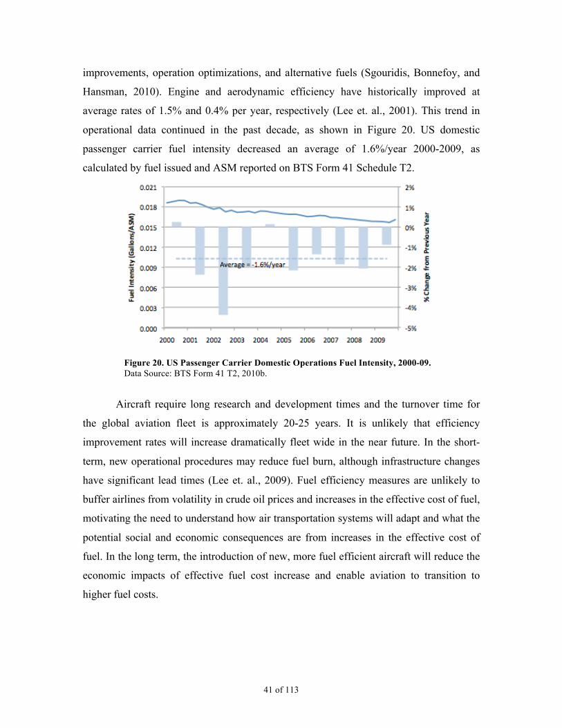
operational data continued in the past decade, as shown in Figure 20. US domestic
passenger carrier fuel intensity decreased an average of 1.6%/year 2000-2009, as
calculated by fuel issued and ASM reported on BTS Form 41 Schedule T2.
Figure 20. US Passenger Carrier Domestic Operations Fuel Intensity, 2000-09. Data Source: BTS Form 41 T2, 2010b.
Aircraft require long research and development times and the turnover time for
the global aviation fleet is approximately 20-25 years. It is unlikely that efficiency
improvement rates will increase dramatically fleet wide in the near future. In the short-
term, new operational procedures may reduce fuel burn, although infrastructure changes
have significant lead times (Lee et. al., 2009). Fuel efficiency measures are unlikely to
buffer airlines from volatility in crude oil prices and increases in the effective cost of fuel,
motivating the need to understand how air transportation systems will adapt and what the
potential social and economic consequences are from increases in the effective cost of
fuel. In the long term, the introduction of new, more fuel efficient aircraft will reduce the
economic impacts of effective fuel cost increase and enable aviation to transition to
higher fuel costs.

42 of 113
Social and Economic Impacts of Reductions in Air Service
Goetz and Sutton (1997) used a core-periphery structure to explain the geographic
effects of deregulation on the airline industry from 1978-1993. Their findings showed
that core centers (the large hubs and international gateways, such as Chicago, Atlanta and
New York) benefited more than the periphery spoke cities from increased air
transportation employment, frequency of service, passenger flow, and lower fares, except
where one or two airlines dominated a hub. If the observed impacts of the fuel price surge
were to become permanent, lasting social and economic effects could occur, continuing
the geographic trends of deregulation.
Airports provide numerous benefits to their region of service, including: reduced
travel time and cost, enable businesses and healthcare procedures requiring time sensitive
shipments, civil defense, stimulation of regional business, access to the national airport
system, and recreation. Economic impacts are described as direct, indirect, induced, and
catalytic. The direct and indirect regional economic impacts of airports can be estimated
using FAA guidelines. These impacts scale with the number of commercial passengers
and airport-based aircraft. In 1992, Butler and Kiernan estimated an airport with 50 based
aircraft induced an annual benefit of $615,500 and provided annual payroll of $304,500,
while an airport with 50 based aircraft and 50,000 annual commercial customers induced
$1,672,500 of annual benefit and $1,827,000 of annual payroll (1992 US$). Reductions
in service and the accompanying passenger traffic to small airports could limit the
financial viability of many airports, depriving inhabitants in the airport’s catchment area
of these benefits.
Malina, Schwab and Wollersheim (2007) used a contingent valuation approach
for a secondary airport in Germany and its catchment area to quantify the catalytic effect
for regional economies that are induced by airports. Their study provided insights as to
which industries benefit the most from the airport and the value companies place on
airports. Ishutkina and Hansman (2008) described the interaction between air
transportation and economic activity in regions throughout the world. By examining links
between economic development and air transportation, they showed how different
regions have developed air transportation systems to generate comparative advantages.
For example, United Arab Emirates’ has diversified its oil-based economy to include
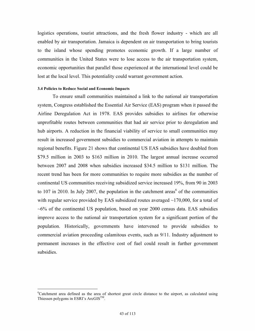
43 of 113
logistics operations, tourist attractions, and the fresh flower industry - which are all
enabled by air transportation. Jamaica is dependent on air transportation to bring tourists
to the island whose spending promotes economic growth. If a large number of
communities in the United States were to lose access to the air transportation system,
economic opportunities that parallel those experienced at the international level could be
lost at the local level. This potentiality could warrant government action.
3.4 Policies to Reduce Social and Economic Impacts
To ensure small communities maintained a link to the national air transportation
system, Congress established the Essential Air Service (EAS) program when it passed the
Airline Deregulation Act in 1978. EAS provides subsidies to airlines for otherwise
unprofitable routes between communities that had air service prior to deregulation and
hub airports. A reduction in the financial viability of service to small communities may
result in increased government subsidies to commercial aviation in attempts to maintain
regional benefits. Figure 21 shows that continental US EAS subsidies have doubled from
$79.5 million in 2003 to $163 million in 2010. The largest annual increase occurred
between 2007 and 2008 when subsidies increased $34.5 million to $131 million. The
recent trend has been for more communities to require more subsidies as the number of
continental US communities receiving subsidized service increased 19%, from 90 in 2003
to 107 in 2010. In July 2007, the population in the catchment areas6 of the communities
with regular service provided by EAS subsidized routes averaged ~170,000, for a total of
~6% of the continental US population, based on year 2000 census data. EAS subsidies
improve access to the national air transportation system for a significant portion of the
population. Historically, governments have intervened to provide subsidies to
commercial aviation proceeding calamitous events, such as 9/11. Industry adjustment to
permanent increases in the effective cost of fuel could result in further government
subsidies.
6Catchment area defined as the area of shortest great circle distance to the airport, as calculated using Thiessen polygons in ESRI’s ArcGISTM.

44 of 113
Figure 21. EAS Subsidies and Continental US Communities Served by EAS. Data Source: Office of Aviation Analysis, 2010.
In 2008, three EAS carriers serving 37 communities ceased operations. 30 EAS
communities were temporarily without air service for up to 10 months, and 6 for a longer
period of time (GAO, 2009). Although the EAS mechanism was able to return service to
these communities, this prolonged interruption likely resulted in social and economic
effects. The number of carriers providing EAS service has declined from 34 in February
1987 to 10 in May 2010. In the event of future shocks to the airline industry it is likely
that small communities will face interruptions in air service. Changes to the EAS
mechanism may be required to mitigate negative impacts.
Nolan, Ritchie, and Rowcroft (2005) examined various schemes to attract air
service in smaller markets, including: direct subsidies, protected route packages, and
guaranteed revenue approaches (e.g. airline travel banks). Using a small network
simulation model, they evaluated each option in terms of social welfare and underlying
agency costs. They found that using revenue guarantees, as opposed to direct subsidies,
reduces the agency problems of adverse selection, opportunism and regulatory capture.
Adverse selection occurs when communities lobbying for regulatory support have an
inherent interest in overstating their need. Cases in which one or more of the parties
abrogates the terms of an agreement demonstrate opportunism (e.g. an air carrier refusing
to provide as many flights as originally promised). Regulatory capture results in the
politician, the regulator, or the firm capturing the control and benefit of the regulatory
process at the cost of the community.

45 of 113
GAO (2003) recommended more flexibility to be built into the EAS program,
including eliminating subsidized service to certain communities that are relatively close
to other larger airports, providing eligible communities with grants to allow them to tailor
air service to unique local needs, and allowing carriers to operate smaller aircraft that are
more suited to local levels of demand. If small communities continue to require subsidies
to maintain air service, Congress will need to decide what level of access to air service is
acceptable and what level of subsidies it is willing to provide. In March 2011, future
funding for EAS was in question. The House version of the FAA Reauthorization and
Reform Act of 2011 proposed phasing out funding for EAS over four years while the
Senate version included reduced funding levels (Darson, 2011). Although non-hub
airports account for 72% of continental US airports with commercial service, they
account for only 9% of departures, which are generally performed in smaller aircraft over
shorter stage lengths, resulting in smaller aggregated environmental impacts than large
jets from large airports. When considering climate change and energy legislation,
Congress will need to weigh the social and economic benefits of air service in small
communities against the limited potential for reductions in environmental impacts.
3.5 Summary
Using the 2004-08 fuel price surge as a natural experiment, it has been shown that
connections to non-hub airports serving small communities were most sensitive to
effective fuel cost increases. It was found that non-hub airports lost 12% of connections,
compared to an average loss of 2.8%, July 2004-08. The complete loss of service July
2007-08 at 70 non-hub airports, representing 14% of continental US airports with
commercial service, resulted in an average driving time of 75 minutes to the next nearest
airport with service for passengers relying on airports no longer with service. It is
believed that reduced access to the national air transportation system had social and
economic effects for small communities. The cessation of operations of Air Midwest and
Big Sky Airlines, the sole carriers serving 20 communities in July 2007, resulted in much
of the volatility in airports with service 2007-08. Regional and commuter airlines were
less able to handle fuel cost volatility during this period as ten declared bankruptcy. To
maintain historic levels of access to the air transportation system, funding for EAS
subsidized routes has doubled since 2003 while the number of continental US

46 of 113
communities serviced by subsidized routes has increased 19% to 107 in 2010. Even
though subsidies have increased, 36 airports were without service for 10 months or longer
following the 2008 fuel price surge. If small communities continue to require increasing
subsidies to maintain air service, Congress will need to decide what level of access to air
service is acceptable, what level of subsidies it is willing to provide, and how flexibility
can be designed into programs to reduce interruptions in air service to small communities
in the future.
Increases in the effective cost of aviation fuel could result from escalating crude
oil prices and environmental driven costs (i.e. from cap and trade schemes or taxes).
Complementary analyses of aircraft fuel efficiency, airline economics, and airfares
provided a basis for understanding some airline decisions during the fuel price surge that
can be extrapolated to examine future trends. Increased effective fuel costs will provide
incentives for airlines to improve fleet fuel efficiency, reducing the environmental effects
of aviation, but may cause an uneven distribution of social and economic impacts as
airline networks adapt. As fuel costs increased 2004-08, use of aging, fuel inefficient
aircraft was reduced while the number of operating turboprops increased. Permanent
effective fuel cost increase will likely lead to increased adoption rates of CO2 mitigating
measures which reduce fuel burn, such as aircraft technology innovations, optimized
operational procedures, and network changes. Benefits due to reductions in the
environmental impacts of aviation may be balanced by social and economic costs.
Government action may be required to determine acceptable levels of access to service as
the air transportation system transitions to higher fuel costs.

47 of 113
CHAPTER 4
4.0 Improving Fleet Fuel Efficiency Through Technology Innovation
In the short- and medium-term, increases in effective fuel costs are expected to
result in higher direct operating costs and airfares, as well as reductions in air service to
markets no longer economical to serve. In the long-term, fleet fuel efficiency can be
improved by replacing old aircraft with fuel-efficient aircraft, reducing the negative
social and economic impacts of increased effective fuel costs. Fuel efficiency
improvements counteract increasing fuel costs and reduce the environmental impact of
aviation. But innovation takes time and aircraft are long-lived assets, resulting in a slow
diffusion of new technologies into the fleet. Further, before a new technology is
implemented in an aircraft, manufacturers must have the economic incentives to
innovate.
In this chapter, historical and projected future aircraft fuel intensity improvements
are reviewed and the dynamics of fleet turnover are discussed. The structure of the single
aisle aircraft market is outlined and the competitive game between manufacturers is
introduced. Two key elements are required to perform the game theory analysis of
aircraft manufacturer competition in Chapter 6: (1) an understanding of the structure of
the game, and (2) an estimation of strategy payoffs. This chapter describes the structure
of the game while Chapter 5 introduces an aircraft program valuation model used to
estimate the payoffs to manufacturers.
4.1 Historical Aircraft Fuel Intensity Improvements
The Breguet range equation can be adapted to demonstrate the levers available to
reduce aircraft fuel burn and CO2 emissions, as shown in Equation 1 (Kar, 2010; adapted
from Lee et. al., 2001):

48 of 113
!
Total CO2 Emissions = (
CO2
Fuel Weight i
)all fuel types
" * (Wempty + W payload ) #{e(
R
V#SFC #
D
L)
$1}all flights using fuel typei
"%
& ' '
(
) * *
Average
Load
Factor
Passenger
Traffic
{Demand}
!
Pax "Avail seats
Pax"
nflights
Avail seats
Fleet Mix
{Aircraft Size}
Empty
Mass
Payload
Mass
Total Fuel of Type i Consumed CO2 Content in Fuel Type i
Range
and
Speed
Sp. Fuel
Consumption
{Propulsion}
Drag/Lift
{Aerodynamics}
Equation 1
Kerosene based jet fuel is currently the only safety certified fuel available in sufficient
quantities. It has a CO2 content of 3.15 kg CO2/kg fuel. The use of alternative jet fuels
with lower fossil carbon contents may result in CO2 emission reductions, but to reduce
the amount of fuel burned, the available levers are (Kar, 2010):
• Weight - reduce the aircraft’s empty weight and the payload mass.
• Engine Efficiency – reduce the specific fuel consumption by improving the
engine efficiency, such as through higher bypass ratios.
• Aerodynamics - increase the lift to drag ratio.
• Average Load Factor – fill flights with more passengers and cargo.
• Fleet Mix - use larger aircraft that take advantage of scale economies to be more
efficient on a seat-mile or ton-mile basis.
• Flight Distance – modify network topology to reduce connections and improve
air traffic control procedures to reduce flight distances.
• Cruise Speed – operate at cruise speeds that minimize fuel burn.
The IPCC (1999) used Figure 22 to demonstrate that jet aircraft fuel efficiency
has improved over time, with current aircraft burning 70% less fuel per seat mile than
early jets. About 40% of the improvement has come from engine efficiency
improvements and 30% from airframe efficiency improvements.

49 of 113
Figure 22. Trend in Transport Aircraft Fuel Efficiency. de Havilland Comet 4 Base Aircraft. Source: IPCC, 1999.
Successive generations of engine technologies have led to reductions in specific
fuel consumption, as shown in Figure 23.
Figure 23. Reduction in Fuel Consumption and CO2 Emissions by Engine Technology. Source: Ferreri, 2003.

50 of 113
Lee et. al. (2001) used BTS operational data to compare historic trends in the
energy intensity of aircraft per available seat kilometre (ASK). Extrapolating the historic
trends, they project energy intensity to decline at an expected rate of 1.2%-2.2% per year,
as shown in Figure 24:
Figure 24. Future Aircraft Energy Usage. Source: Lee et. al., 2001.
Using operational data, Babikian et. al. (2002) demonstrated that regional aircraft
are 40-60% less fuel efficient than narrow- and wide-body aircraft, and that regional jets
are 10-60% less fuel efficient than turboprops, as shown in Figure 25. The disparities in
fuel efficiency were largely explained by differences in operations as opposed to
technology levels. Regional aircraft operate with lower load factors and perform fewer
miles over which to spread the fixed costs of taxiing, takeoff and climb. To improve fleet
fuel efficiency, it is not enough to improve technology in only the largest wide body
aircraft. Operations and technology levels in narrow body and regional jets must also
improve.
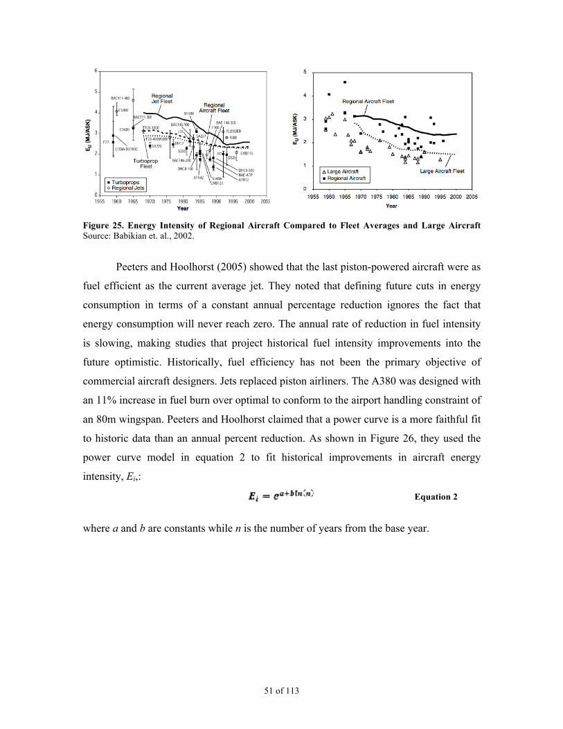
51 of 113
Figure 25. Energy Intensity of Regional Aircraft Compared to Fleet Averages and Large Aircraft Source: Babikian et. al., 2002.
Peeters and Hoolhorst (2005) showed that the last piston-powered aircraft were as
fuel efficient as the current average jet. They noted that defining future cuts in energy
consumption in terms of a constant annual percentage reduction ignores the fact that
energy consumption will never reach zero. The annual rate of reduction in fuel intensity
is slowing, making studies that project historical fuel intensity improvements into the
future optimistic. Historically, fuel efficiency has not been the primary objective of
commercial aircraft designers. Jets replaced piston airliners. The A380 was designed with
an 11% increase in fuel burn over optimal to conform to the airport handling constraint of
an 80m wingspan. Peeters and Hoolhorst claimed that a power curve is a more faithful fit
to historic data than an annual percent reduction. As shown in Figure 26, they used the
power curve model in equation 2 to fit historical improvements in aircraft energy
intensity, Ei,:
Equation 2
where a and b are constants while n is the number of years from the base year.

52 of 113
Figure 26. Aircraft Fuel Efficiency Trends and Projections. Source: Peeters and Hoolhurst, 2005.
Using sales-weighted average aircraft fuel burn, Rutherford and Zeinali (2009)
demonstrated that the average aircraft fuel efficiency has improved by only ~50% since
the first jets, while efficiency gains have slowed to 0.0% since 2000, as shown in Figure
27. The reduction in annual efficiency gains is correlated with low fuel prices from 1987
to 2004 and a tripling in the average age of aircraft and engine manufacturer production
lines since 1989. Rutherford and Zeinali conclude that fuel costs have not been sufficient
to stimulate increased aircraft efficiency, suggesting that a CO2 standard applying to
newly built aircraft is more likely to reduce emissions. But the 1980s marked a period of
fierce competition between manufacturers and rapid fleet fuel efficiency improvements.
Therefore, We hypothesize that competition between aircraft and engine manufacturers is
a key driver of innovation resulting in fuel efficiency improvements.

53 of 113
Figure 27. Sales-Weighted Average Jet Aircraft Fuel Burn, 1960-2008. Source: Rutherford and Zeinali, 2009.
4.2 Future Potential Fuel Intensity Improvements
Tube and wing designs have dominated commercial aircraft since the 1950s,
while engine technology innovations have led to three product cycles during the jet era,
as shown in Figure 28.
Figure 28. Life Cycles and Replacement of Jet Aircraft Class Product. Source: Ferreri, 2003.
54 of 113
Dominant designs emerge from a process of experimentation and competition
within a product class. As a synthesis of a number of proven concepts, the dominant
design becomes locked-in to future designs and consumer expectations. Tushman and
Anderson (1986) wrote: …technology evolves through periods of incremental change punctuated by technological breakthroughs that either enhance or destroy the competence of firms in an industry. These breakthroughs, or technological discontinuities, significantly increase both environmental uncertainty and munificence….while competence-destroying discontinuities are initiated by new firms and are associated with increased environmental turbulence, competence-enhancing discontinuities are initiated by existing firms and are associated with decreased environmental turbulence. These effects decrease over successive discontinuities. Those firms that initiate major technological changes grow more rapidly than other firms. In the next jet aircraft product cycle, incumbent manufacturers have an
opportunity to innovate. By building on their past successes and implementing
technology innovations in new designs, incumbents can raise entrance barriers and
prevent increased competition. If they choose not to innovate, incumbent manufacturers
may lose their technological superiority and significant market share to new entrants.
Although fuel efficiency is not the sole aircraft design criteria, with the expectation of
increasing fuel costs and pressure to reduce aviation’s environmental impacts it is likely
that fuel efficiency will increasingly be the critically important design criterion. While
safety will always be aviation’s primary concern, it is probable that the next
discontinuous aircraft design change will be a step improvement in fuel efficiency.
NASA’s Environmentally Responsible Aviation (ERA) project aims to assess
vehicle concepts and enabling technologies that have the potential to mitigate aviation’s
impact on the environment. Table 6 outlines the project’s goals for subsonic vehicles.

55 of 113
Table 6. NASA’s Environmentally Responsible Aviation (ERA) Project Goals for Subsonic Vehicles “N” - the current generation of commercial aircraft. “N+1” - the next generation, and so forth.
In the first stage of the NASA ERA project, MIT, Boeing, GE Aviation, and
Northrop Grumman developed conceptual designs for N+3 vehicles. MIT developed two
designs that met the NASA goals: (1) a double-bubble, and (2) a hybrid wing body. The
D8 Series double-bubble was a 180-seat advanced tube and wing design that could fulfill
the current role of Boeing’s 737-800. It incorporated a lifting nose, embedded aft engines,
and a reduced operational Mach number allowing for nearly unswept wings. The H3
Series was a more radical 350-seat design with a payload and range comparable to
Boeing’s 777-200LR. As a triangular-shaped hybrid wing body aircraft, the H3 blended a
wider fuselage with the wings for improved aerodynamics. The center body created lift,
eliminating the need for a tail to balance the aircraft (Greitzer et. al., 2010). Non-
traditional aircraft designs would be a risky and costly project for a private firm to
undertake. New technologies need to be developed, manufactured, tested, and safety
certified. This creates significant financial and technical barriers to implementation of
such discontinuous technologies.
Kar (2010) demonstrated that there are a number of technologies at various stages
of technology readiness that have the potential to reduce fuel burn. In the near-term, new
engine technologies, aerodynamic improvements, and weight reduction opportunities
exist that could result in substantial fuel burn improvements in retrofitted or new aircraft.
In the long-term, fuel burn reduction potential is even greater. Table 7 outlines a selection
of the technologies identified.

56 of 113
Table 7. Selection of Technologies to Improve Fuel Efficiency. Source: Kar, 2010.
Near-Term <5 years
Long-Term >5 years
Propulsion High bypass ratio engines Open rotor engines Geared turbofan engines Aerodynamics Winglets Hybrid laminar flow Riblets High aspect ratio wings Laminar nacelles Weight Composites Reduced OEW
Figure 29 shows a temporal representation of the 41 CO2 mitigating measures identified
by Kar (2010). The amount of time required to reach market saturation is called the
diffusion time while the start time represents the estimate of the measure’s year of entry
into service. The area of each bubble represents the percent potential CO2 emissions
reduction.
Figure 29. Distribution of Mitigating Measures’ Start and Diffusion Times. Source: Kar, 2010.
While it is likely that technologies either do, or will, exist to substantially reduce
aircraft fuel burn, they will only be implemented if they are economically feasible.
Retrofitting in-service aircraft with non-safety required equipment has generally not
proven economical. Updating technologies on current in-production aircraft leads to
incremental fuel efficiency improvements, but engineers are constrained by previous
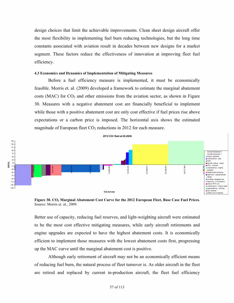
57 of 113
design choices that limit the achievable improvements. Clean sheet design aircraft offer
the most flexibility in implementing fuel burn reducing technologies, but the long time
constants associated with aviation result in decades between new designs for a market
segment. These factors reduce the effectiveness of innovation at improving fleet fuel
efficiency.
4.3 Economics and Dynamics of Implementation of Mitigating Measures
Before a fuel efficiency measure is implemented, it must be economically
feasible. Morris et. al. (2009) developed a framework to estimate the marginal abatement
costs (MAC) for CO2 and other emissions from the aviation sector, as shown in Figure
30. Measures with a negative abatement cost are financially beneficial to implement
while those with a positive abatement cost are only cost effective if fuel prices rise above
expectations or a carbon price is imposed. The horizontal axis shows the estimated
magnitude of European fleet CO2 reductions in 2012 for each measure.
Figure 30. CO2 Marginal Abatement Cost Curve for the 2012 European Fleet, Base Case Fuel Prices. Source: Morris et. al., 2009.
Better use of capacity, reducing fuel reserves, and light-weighting aircraft were estimated
to be the most cost effective mitigating measures, while early aircraft retirements and
engine upgrades are expected to have the highest abatement costs. It is economically
efficient to implement those measures with the lowest abatement costs first, progressing
up the MAC curve until the marginal abatement cost is positive.
Although early retirement of aircraft may not be an economically efficient means
of reducing fuel burn, the natural process of fleet turnover is. As older aircraft in the fleet
are retired and replaced by current in-production aircraft, the fleet fuel efficiency

58 of 113
improves. But, if in-production aircraft technology levels remain constant, operating fleet
fuel efficiency improvements slow as all aircraft in the fleet approach the same
technology level. Kar (2010) found that the early adoption of available technology, as
opposed to waiting and delaying entry for more fuel-efficient technologies, has a greater
potential to improve fleet fuel efficiency by 2050. With operating lifetimes of 20-25
years, significant changes to the average fleet fuel efficiency require a combination of
step improvements in the fuel burn of new models and an acceleration of adoption of new
models.
Morrell and Dray (2009) analyzed fleet turnover and the incorporation of new
technologies. They found that airline purchase decisions have historically not been
affected by fuel prices when the selection of aircraft types available remains constant.
However, the mean fuel burn of new aircraft orders is strongly affected by the
introduction of new aircraft models with significantly lower fuel burn. This finding
suggests that influencing the rate of technology development may be an effective policy
lever for reducing emissions via fleet turnover. Single aisle aircraft currently make up
61% of the world’s jet fleet and 68% of 2010-29 forecasted deliveries (Boeing, 2010a).
As the largest lever, the single aisle market was investigated to determine what factors
and policies might lead to the introduction of new aircraft models with step
improvements in fuel efficiency.
4.4 Single Aisle Aircraft Market Structure
As an industry with economies of scale that requires large capital investments,
high technical capabilities, and a worldwide service network, large commercial aircraft
manufacturing is naturally concentrated to a small number of competitors (Busch, 2001).
The 100+ seat commercial market has historically been split between the American
manufacturers (Boeing, McDonnell-Douglas, and Lockheed) and the European Airbus
consortium, as shown in Figure 31.

59 of 113
Figure 31. Large Commercial Aircraft Manufacturer Market Shares by 100+ Seat Jetliner Deliveries, 1960-2009. Date Source: Airbus, 2010b; Boeing, 2010b.
Since Boeing’s purchase of McDonnell-Douglas in 1997, Airbus and Boeing have
competed in a global duopoly. Large barriers to entry exist which protect the incumbents
from new competition. The cost of developing a new aircraft ranges from estimates of $3
to $14 billion (depending on the aircraft size and technology level) and requires expertise
only developed over long periods of time. Production learning effects result in unit costs
dropping on the order of 20% every time the quantity produced doubles, creating
significant unit cost advantages for aircraft with long production runs (Benkard, 2000).
Further, airlines purchasing new aircraft demand low operating costs and competitive
pricing. Fleet commonality reduces operating and maintenance costs, as well as spare part
inventories, providing incentives for airlines to lock-in to one aircraft family. In order to
maintain market share in a segment, manufacturers are forced to develop aircraft with
essentially equivalent performance. To gain market share, significant performance
improvements are required to overcome the switching costs of airlines locked-in to one
product family.
Boeing and Airbus compete in market segments defined by the aircraft’s range
and seating capacity, which vary from 2000 to 8000+ miles and 100 to 500+ seats.
Narrow body aircraft serve short- and medium-haul routes while wide body aircraft
generally serve cross- and inter-continental routes. Both companies recently updated their
large wide bodies with the introduction of Airbus’s A380 in 2007 and the expected first

60 of 113
delivery of Boeing’s 747-8 in 2011. In the medium wide body market segment, the
manufacturers are entering a battle between Boeing’s 787 Dreamliner and Airbus’s larger
A350 XWB, with first deliveries expected in 2011 and 2013, respectively. Manufacturers
generally respond to each other’s moves to prevent an inferior aircraft in a market
segment from losing market share and profit potential. As both manufacturers have a
complete product line and have performed significant updates to their wide body aircraft
families, the next area of competition is likely the narrow body, single aisle segment -
Boeing’s 737 and Airbus’s A320 families.
Boeing’s 737 first entered service in 1968. A variety of derivative aircraft based
on the initial design, with different ranges and seating capacities, have been produced
over the years. Members of the Next Generation 737 family were launched in the late
1990s and early 2000s with updated engines, cabin interiors, and flight deck avionics as
well as winglets and changes to the airframe. Airbus entered its A320 family into service
in 1988. The aircraft’s fuselage has been stretched and shrunken to fill different market
niches with the introduction of the A321, A319, and A318. A variety of engines have
been used on the Airbus airplanes allowing for incremental improvements in fuel
efficiency. Figure 32 shows a timeline of upgrades performed to both manufacturers’
single aisle product lines over the past 30 years.
Figure 32. Narrow Body Single-Aisle Jet Aircraft, 1980-2010. Source: Boeing, 2010c.

61 of 113
If one manufacturer develops a superior aircraft, its competitors risk losing market
share, as shown in Figure 33. In the 150-185 seat single aisle short- to medium-range
market segment, Boeing’s 727-200 enjoyed a monopoly until the MD-80 entered service
in 1980 with an estimated 37% fuel burn improvement at the R1 range7 (not shown in the
figure). Boeing’s 737-400 and Airbus’s A320 entered service in 1988, offering
significant performance improvements over the MD-80. McDonnell Douglas exited the
market in 1997 leaving the two remaining manufacturers to split the market. Since the
late 1990s when Boeing introduced the 737-800 and 737-900, the manufacturers have
performed incremental improvements on their existing product lines.
Figure 33. Single Aisle, 150-185 Seat Market Shares and Fuel burn Performance, 1980-2009. Data Source: Airbus, 2010b; Boeing, 2010b; Piano-X.
New competition in the single aisle markets may be on the horizon. Figure 34
demonstrates that while only a few firms enjoy the technical competency, financial
resources, and market control that allow them to carry on the development of an aircraft
program in all phases, the number of competitors expands moving down the productive
pyramid (Ferreri, 2003). As regional aircraft manufacturers and major structure sharing
suppliers develop design and production capabilities, they may decide to compete with
the incumbents in the large commercial aircraft market segments (Bediér et. al., 2008).
Embraer’s E195 encroaches on the 100+ seat market while Bombardier’s CSeries is due
7 R1 range is the maximum aircraft range after which payload must be sacrificed to gain additional range.
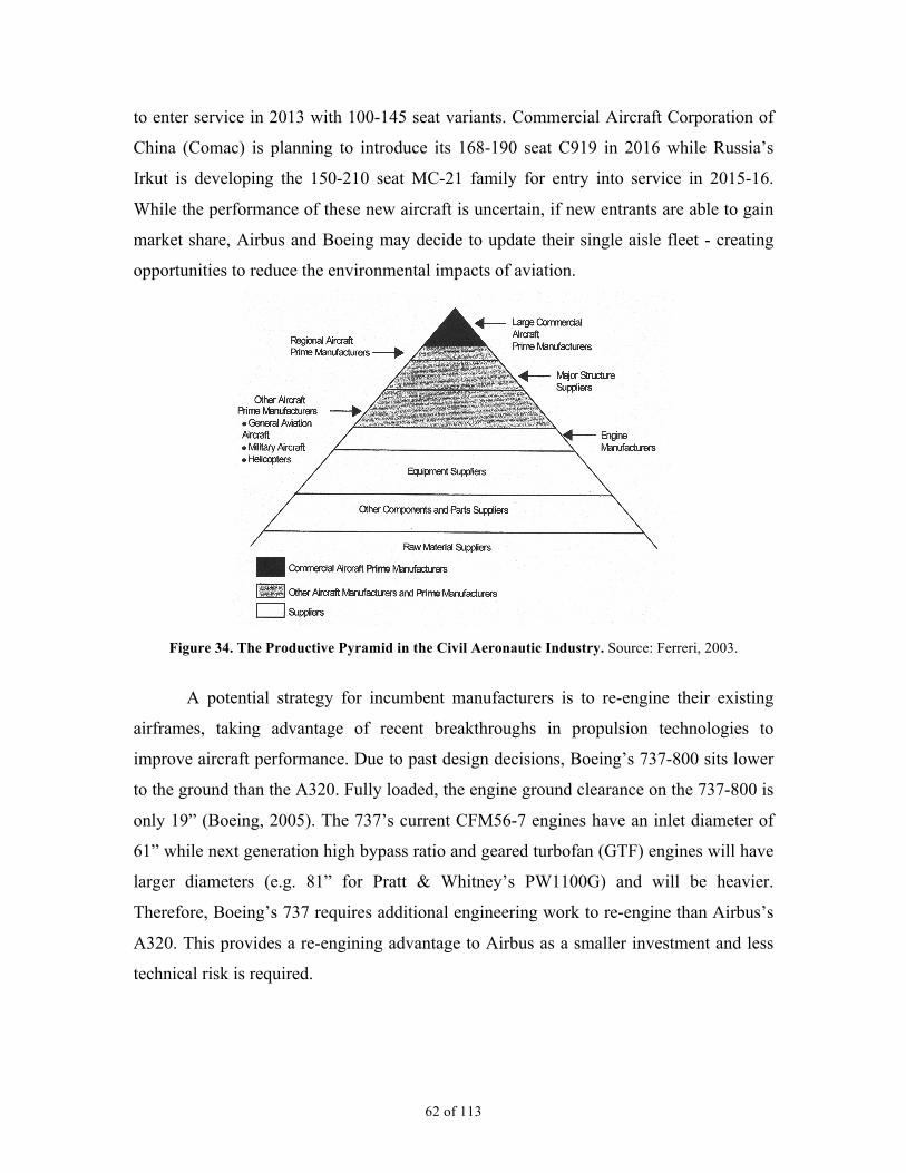
62 of 113
to enter service in 2013 with 100-145 seat variants. Commercial Aircraft Corporation of
China (Comac) is planning to introduce its 168-190 seat C919 in 2016 while Russia’s
Irkut is developing the 150-210 seat MC-21 family for entry into service in 2015-16.
While the performance of these new aircraft is uncertain, if new entrants are able to gain
market share, Airbus and Boeing may decide to update their single aisle fleet - creating
opportunities to reduce the environmental impacts of aviation.
Figure 34. The Productive Pyramid in the Civil Aeronautic Industry. Source: Ferreri, 2003.
A potential strategy for incumbent manufacturers is to re-engine their existing
airframes, taking advantage of recent breakthroughs in propulsion technologies to
improve aircraft performance. Due to past design decisions, Boeing’s 737-800 sits lower
to the ground than the A320. Fully loaded, the engine ground clearance on the 737-800 is
only 19” (Boeing, 2005). The 737’s current CFM56-7 engines have an inlet diameter of
61” while next generation high bypass ratio and geared turbofan (GTF) engines will have
larger diameters (e.g. 81” for Pratt & Whitney’s PW1100G) and will be heavier.
Therefore, Boeing’s 737 requires additional engineering work to re-engine than Airbus’s
A320. This provides a re-engining advantage to Airbus as a smaller investment and less
technical risk is required.

63 of 113
4.5 Structure of the Competitive Game
Game theory frameworks have been used in the past to analyze competition
between aircraft manufacturers. Brander and Spencer (1985) showed how government
subsidies could be used to change the initial conditions of games between non-
cooperative international rivals. Krugman (1987) used hypothetical payoff matrices to
show how government subsidies could enable domestic firms to increase profits in excess
of the subsidy amounts by deterring foreign entry and allowing domestic firms to capture
excess returns, increasing social welfare. A game theory analysis enables the discovery of
the Nash equilibrium of multiple, competing players’ who all act in their own best
interests. Understanding how competition impacts the decision to invest in new aircraft
designs can assist policy makers in developing plans of action to improve aviation’s fuel
efficiency.
As both Boeing and Airbus have existing in-production single aisle aircraft, the
game has been altered since the economists analyzed it in the 1980s. Incumbent
manufacturers have four generic strategies: (1) maintain their existing product lines, with
incremental improvements over time, (2) re-engine their existing airframes, providing
superior performance improvement, (3) develop new, clean sheet design aircraft that offer
the greatest fuel burn improvements, or (4) exit the market. Based on historical data,
incremental improvements to an aircraft generally amount to ~1%/annual fuel intensity
reductions. Re-engining Airbus’s A320 or Boeing 737-800 is expected to offer up to 15%
fuel savings (Airbus, 2010a). A new aircraft with a clean sheet design would offer a fuel
efficiency improvement on the order of 25% (ACARE, 2008; Morrell and Dray, 2009).
As technologies mature, clean sheet design aircraft in the future will offer greater
efficiency, with expected improvements on the order of 70% by 2040 (Kar, 2010).
NASA’s ERA goals include developing technologies that will enable 70% or better fuel
burn performance on clean sheet design aircraft by 2025. Therefore, in the long term,
there is a performance advantage to delay the design of a new aircraft. Due to payback
periods on the order of 10-15 years for large commercial aircraft programs, when a
manufacturer commits to a new aircraft, they lock-in to the technology level for the
duration of the program, enabling only incremental improvements. Figure 35 shows that
if Manufacturer A decides to re-engine in 2010, the aircraft is expected to enter service

64 of 113
around 2015, providing a performance advantage over Manufacturer B’s product. But, if
Manufacturer B decides to develop a new aircraft around 2015, they would gain the
performance advantage when it enters service around 2020. Locking into a technology
may leave a competitor vulnerable to their aircraft being obsolete five or ten years later -
around the same time manufacturers hope for their programs to become profitable and
benefit from reduced production unit costs through learning effects. Aircraft that have
superior performance gain market share and yield higher sale prices. Although
manufacturers can always purchase market share by dropping sale price, this strategy
reduces profit margins.
Figure 35. Potential Fuel Burn Improvements of Future Technologies.
Uncertainties in future demand and fuel prices impact the expected value of an
aircraft program. The demand for new aircraft is dependent on the profitability of airlines
and is therefore volatile, impacted by GDP growth, macroeconomic cycles, and passenger
preferences (Sgouridis, 2007). Manufacturers must build production facilities and supply
chains with the flexibility to meet expected demand. Optimistic forecasts expose the
manufacturer to downside risks that may result in severe financial consequences while
overly pessimistic forecasts limit the potential upside of the program. Operating cost
savings is a major selling point of new aircraft programs, but the magnitude of operating
cost savings is partially dependent on future fuel prices. Fuel prices are volatile, resulting
in uncertainty in the value of efficiency improvements and prices manufacturers can
obtain for increased aircraft technology levels.

65 of 113
In Chapter 6, two types of games are analyzed: (1) static games in which the
manufacturer’s decision space is limited to maintaining their product lines, re-engining
their current aircraft, or developing a new aircraft, and (2) dynamic games in which
manufacturers update their decisions at 5-year increments, based on the evolution of fuel
prices and demand for single aisle aircraft. Figure 36 outlines the decision space in both
types of games. It is assumed that there is a 5-year delay from when a decision is made to
when the aircraft enters service. Therefore, a decision to develop a new aircraft includes
the production and sale of the existing aircraft for 5-years until the new aircraft enters
service. In the dynamic game, it is assumed that a manufacturer would produce a re-
engined aircraft for 10-years to receive a sufficient payback on their investment. In each
case, it is assumed that a player’s moves in the game terminate when they decide to
develop a new aircraft. A 20-year period is used for the static games to correspond to the
manufacturer demand forecasts and oil price forecasts while a 30-year period is used for
the dynamic games to enable a sufficient payback period for new aircraft introduced in
later stages.
Figure 36. Structure of the Static and Dynamic Games Analyzed.
4.6 Summary
Chapter 4 reviewed historical improvements in aircraft fuel efficiency. Fleet wide
fuel efficiency improvements will only be obtained by the introduction of new single
aisle aircraft with step performance improvements. New technologies have the potential

66 of 113
to create a discontinuity in the product cycle that offers opportunities for new entrants to
compete or incumbents to solidify their hold on the market. Aviation’s marginal
abatement cost (MAC) curve was introduced, demonstrating that although the natural
process of fleet turnover has a long time constant, it is an economically efficient approach
to improving fleet fuel efficiency. Before new aircraft offering step fuel efficiency
improvements are produced, manufacturers must have the incentives to innovate. The
history of competition in the single aisle market segment was reviewed to understand the
structure of the game that manufacturers are faced with in their current decisions to
maintain, re-engine, or develop a new single aisle aircraft. Before proceeding with the
static and dynamic game analyses, an aircraft program valuation model is introduced in
Chapter 5 that will be used to estimate the manufacturers’ payoffs for the game theory
analysis in Chapter 6.

67 of 113
CHAPTER 5
5.0 Methodology for Aircraft Program Valuation
A game theory analysis is rooted in determining: (1) the structure of the game,
and (2) the payoffs to each player. The structure of the game was outlined in Chapter 4
using a historical analysis of aircraft fuel efficiency improvements and manufacturer
competition in the single aisle aircraft market. This chapter develops an aircraft program
valuation model to estimate the payoffs for the manufacturers’ strategies under varying
market conditions. Following the principle of Occam’s razor, a simple model is
constructed to avoid unnecessary complexity, improving our ability to understand its
behaviour. Aircraft manufacturers keep much of their production and sales financial data
proprietary to protect competitive interests. Therefore, there is uncertainty in the model’s
input parameters. The purpose of this aircraft program valuation model is to determine
the correct rank ordering of manufacturers’ generic strategy payoffs in expected value
terms under the different scenarios investigated in Chapter 6. We make no assertions
concerning the validity of the absolute value of payoffs estimated, but only their rank
ordering. An organization with access to more complete financial data could develop an
improved valuation model and use the framework of analysis developed in Chapters 4
and 6 to yield more accurate cardinal estimates of the manufacturer payoffs.
How manufacturers make the business case for new aircraft programs is discussed
in Section 5.1. The aircraft program valuation model is developed in Section 5.2. A
sensitivity analysis is conducted in Section 5.3 to determine whether the aircraft program
valuation model is robust and how altering the model’s input parameters impact the rank
ordering of payoffs. The chapter is summarized in Section 5.4.

68 of 113
5.1 Making the Case for New Aircraft Programs
Successful aircraft programs require longevity to achieve efficient production
volumes in the face of constantly changing market conditions, competitive actions, and
technological alternatives. Steiner (1982) listed the key drivers for program decisions as:
market needs and timing, government actions and priorities, competitor actions,
technology readiness, and fiscal considerations. Often decisions made become
irreversible due to program cost penalties. Therefore, it is critical to make decisions that
will yield the highest payoff, given all technical, political, and economic variables in the
problem, as well as their associated uncertainty.
Previous works highlight the need to consider more than just the technical aspects
of an aircraft program when making product line decisions. Mavris and Birney (2002)
outlined the need to link the engineering and business sides of a program to provide
decision-makers with a clearer understanding of payoffs and risk. Markish (2002)
developed an aircraft program valuation model that combined a performance model, a
development and manufacturing cost model, and a revenue model with a dynamic
programming algorithm to account for uncertainty in future market conditions,
demonstrating the usefulness of design based on maximum value to the aircraft
manufacturer. Peoples (2004) used a multidisciplinary design optimization (MDO)
approach to assess aircraft performance, finances, and business risk in aircraft program
design. Justin et. al. (2010) are working towards a game-theoretic and real-options based
method that will optimize research and development strategies and properly value large
development projects. The aircraft program valuation model developed in this report
estimates the financial payoffs of aircraft programs to incorporate strategic factors into
aircraft program decisions using game theory. Further work is needed to integrate
technical requirements with the financial and strategic aspects of the problem.
Before deciding to pursue an aircraft program, manufacturers must close the
business case. The right aircraft must target the broadest market segment and rely on a
level of technology that makes production costs reasonable while offering performance
improvements that competitors will have difficulty exceeding. An aircraft design that
includes technologies not yet at an appropriate readiness level will lead to excessive

69 of 113
program delays and cost overruns while a program not ambitious enough will open
opportunities for competitors to capture market share by producing a superior product.
A number of figures of merit are commonly used to value and compare
investment options. These include the payback period, internal rate of return (IRR), cost-
benefit ratio, and net present value (NPV). Each metric has drawbacks and benefits. Net
present value enables cash flows over multiple years to be compared while recognizing
the time value of money through the selection of a discount rate. Expected net present
value, E(NPV), incorporates the uncertainty of NPV calculations by taking the
probability weighted mean of NPV under a range of future scenarios. It is likely that
manufacturers make aircraft program decisions in expected terms using NPV
calculations. Therefore, this metric was selected as the manufacturers’ objective functions
used to calculate payoffs for the game theory analysis in Chapter 6.
5.2 Aircraft Program Valuation Model
As in Irwin and Pavcnik (2004), the objective function of manufacturers is
assumed to be the net present value of expected profits:
! ft = Et " t qt (p) pt ! ct( )( )+ Itt=s
n
"#
$%
&
'(
Equation 3
where Et is the expectation operator conditional on information at time t, n is the number
of periods included in the analysis, δ is the discount factor, qt is the quantity of aircraft
sold (which is a product of the firm’s market share and total market size), pt is the sale
price of the aircraft, ct is the variable cost of production, and I is the nonrecurring
investment required. This objective function is expected for nongovernmental firms
operating in market economies. Firms operating in different home country market
structures may choose different objective functions, but this complexity is not examined.
A symmetric duopoly is assumed in which firm’s are risk neutral and identical, except for
the investment required to re-engine (as discussed in Section 4.4). The static analysis was
limited to a 20-year period as manufacturers release 20-year demand forecasts and
discounting reduces the present value of future cash flows, while the dynamic game was
extended to a 30-year period to enable manufacturers to book revenues from aircraft that
enter into service at later stages in the game. The periods of analysis were broken into

70 of 113
five-year stages to reduce the number of future states considered, making the problem
tractable. Forecasted demand and fuel prices represent average values over the course of
a business cycle. In the following subsections, the objective function in equation 3 is
expanded and assumptions are outlined. The model input parameters are summarized in
Table 14.
Nonrecurring Investments
Aircraft program nonrecurring investments consist of the research, development,
testing and evaluation (RDT&E) of the aircraft. This includes the design, prototypes,
flight testing, production facility construction, and tooling that is required to produce the
first plane that enters commercial service. While this analysis assumes symmetric firms,
due to past design decisions, Boeing’s 737 requires additional engineering work to re-
engine. Therefore, it was assumed that Player B requires a $3 billion investment to re-
engine its aircraft, while Player A only requires a $1.5 billion investment. New aircraft
development programs are much more costly, likely in the range of $10 billion for the
single aisle market (Rothman, 2010). It was assumed that nonrecurring costs are
distributed over one five-year stage in the model. Although designing and testing a new
aircraft is a more complex task than re-engining an existing airframe, the model is broken
into 5-year periods to reduce the number of feasible states explored. Estimates of the
investment required were taken from industry press, based on historical programs.
Recurring Production Costs
Recurring costs of manufacturing aircraft are subject to a learning curve that
incentivizes manufacturers early in a program to produce more, reducing unit production
costs for the remainder of the program. Raymer (2006) uses the learning curve model:
!
cqi = c1qiln " / ln 2 Equation 4
where cqi is the unit production cost of the ith unit produced, c1 is the theoretical first unit
cost (TFUC), qi is the number of units produced, and β is the learning curve slope.
The learning curve slope has been estimated to be between 75% and 95%, with
80% generally accepted based on empirical analysis and expert opinion (Benkard, 2004;
Irwin and Pavcnik, 2004). The theoretical first unit cost was estimated using the DAPCA

71 of 113
IV model, developed by the RAND Corporation using a statistical analysis of past
commercial and military aircraft programs (Raymer, 2006). The estimated unit cost of the
100th aircraft produced was used to estimate the theoretical unit cost of the first based on
the learning curve slope assumption, in the same manner as Markish (2002).
The initial quantity of units produced for the maintain strategy was estimated
from historical deliveries. To the end of 2009, Boeing had delivered 1806 737-800s while
Airbus had delivered 2257 A320s. For the re-engine strategy, it was assumed that the
manufacturer would benefit from significant learning effects due to a long history of
producing the air frame, but the learning curve would be reset to some lower number of
units produced due to the design and production changes required. The initial quantity of
units produced for the re-engine strategy was set at a level where the estimated unit
production cost approximated sale price.
Demand Forecast
Narrow body aircraft deliveries are cyclical, with high volatility, as shown in
Figure 37:
Figure 37. Narrow Body Deliveries, 1990-2009. Data Source: Airbus, 2010b; Boeing, 2010b.
Figure 38 shows that the percentage change in annual deliveries has been volatile over
the past 20 years, around the mean annual growth rates of 10% for A320s and 5.5% for
737s. The business cycles in the 1990s led to much more dramatic changes in yearly

72 of 113
deliveries than in the 2000s, suggesting that manufacturers have taken steps to reduce the
classic supply chain bullwhip effect that was present in earlier decades (Sgouridis, 2007,
p. 322).
Figure 38. Annual Percent Change in 737 and A320 Deliveries, 1990-2009. Data Source: Airbus, 2010b; Boeing, 2010b.
The global demand for single aisle aircraft was forecasted as average yearly
deliveries, for each five-year stage, using a recombinant binomial lattice model, as shown
in Table 8. For each stage of the lattice model, the average demand over the next five-
year stage (i.e. the state, S) was assumed to either increase by amount u or decrease by
amount d, with probability p or 1-p, respectively. Repeating these calculations for each
state, in each stage, yielded a cone of possible demand states and the forecasted
probability of each demand state occurring. The values for u, d, and p were estimated
from historical delivery data using the formulas (Chance, 2007):
!
u = e" #t
!
d = e"# $t
!
p =e"#t $ du $ d
Equation 5
where σ is the delivery variance, ν is the expected mean growth rate of deliveries, and Δt
is the number of periods. The expected deliveries per year for each stage in the lattice
model was the probability weighted average of the stage’s demand states. This method

73 of 113
limited the number of states to explore in the model, but recognized the uncertainty
inherent in forecasting demand over 20 years.
The variance was calculated from the 2000-09 deliveries of MD-80/90, Boeing
737-800/900 and Airbus A320. High and low estimates were calculated using the periods
1990-2009 and 2005-09. The mean growth rate was calculated so that the expected
deliveries over the next 20 years equaled the average of the Airbus and Boeing 2010-
2029 single aisle market forecasts. The high and low estimates of the mean growth rate
were calculated using the two manufacturer’s independent forecasts. Each state of the
lattice model in Table 8 represents the average expected deliveries over each five-year
stage in the years indicated. The initial state represents the average deliveries in the 2005-
09 period.
Table 8. Base Case Aircraft Demand Binomial Lattice Model Stage 0 Stage 1 Stage 2 Stage 3 Stage 4 2005-09 2010-14 2015-19 2020-24 2025-29
Aircraft Deliveries/Year 391 738 1393 2630 4965 207 391 738 1393 110 207 391 58 110 31
Probability 100% 47% 22% 10% 5% 53% 50% 35% 22% 28% 40% 37% 15% 28% 8%
Expected Deliveries/Year 391 455 530 617 718 Total Deliveries, 2010-2029 11,599
Jet Fuel Price Forecast
The expected price of jet fuel influences airlines willingness to invest in fuel burn
reducing technologies. It was assumed that if fuel prices are expected to escalate, airlines
will be more willing to invest in new aircraft that reduce fuel burn, as discussed in
Section 3.3. Therefore, the expected price of fuel influences the prices airlines are willing
to pay for new aircraft and the amount of risk manufacturers are willing to take to
implement fuel efficiency technologies in new aircraft. Jet fuel prices were modeled in
the same manner as the demand for aircraft using a binomial lattice model. The mean
growth rate was taken from the Energy Information Administration’s (EIA) 2010 Annual

74 of 113
Energy Outlook while the variance was determined from historical jet fuel prices (ATA,
2010a). High and low estimates were taken from the EIA oil price scenarios.
Table 9. Base Case Jet Fuel Price Binomial Lattice Model Stage 0 Stage 1 Stage 2 Stage 3 Stage 4 2005-09 2010-14 2015-19 2020-24 2025-29 Jet Fuel Price/Gallon $2.24 $4.58 $9.35 $19.12 $39.07 $1.10 $2.24 $4.58 $9.35 $0.54 $1.10 $2.24 $0.26 $0.54 $0.13
Probability 100% 42% 18% 7% 3% 58% 49% 31% 17% 34% 42% 36% 20% 33% 11% Expected Fuel Price $2.24 $2.56 $2.92 $3.33 $3.80
Aircraft Lifecycle Cost Analysis
New aircraft often fetch a higher sale price to compensate manufacturers for the
risk of increased technology levels. From an airline perspective, the benefits of advanced
technology come from reductions in fuel and maintenance costs over the course of the
aircraft’s operating life, as shown in Figure 39.
Figure 39. The Benefits of Advanced Technology – Fuel Related Cost Savings. Source: Ferreri, 2003.
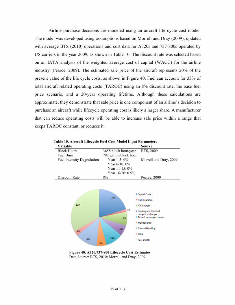
75 of 113
Airline purchase decisions are modeled using an aircraft life cycle cost model.
The model was developed using assumptions based on Morrell and Dray (2009), updated
with average BTS (2010) operations and cost data for A320s and 737-800s operated by
US carriers in the year 2009, as shown in Table 10. The discount rate was selected based
on an IATA analysis of the weighted average cost of capital (WACC) for the airline
industry (Pearce, 2009). The estimated sale price of the aircraft represents 20% of the
present value of the life cycle costs, as shown in Figure 40. Fuel can account for 33% of
total aircraft related operating costs (TAROC) using an 8% discount rate, the base fuel
price scenario, and a 20-year operating lifetime. Although these calculations are
approximate, they demonstrate that sale price is one component of an airline’s decision to
purchase an aircraft while lifecycle operating cost is likely a larger share. A manufacturer
that can reduce operating costs will be able to increase sale price within a range that
keeps TAROC constant, or reduces it.
Table 10. Aircraft Lifecycle Fuel Cost Model Input Parameters
Variable Source Block Hours 3658 block hour/year BTS, 2009 Fuel Burn 792 gallon/block hour Fuel Intensity Degradation Year 1-5: 0%
Year 6-10: 0% Year 11-15: 0% Year 16-20: 0.5%
Morrell and Dray, 2009
Discount Rate 8% Pearce, 2009
Figure 40. A320/737-800 Lifecycle Cost Estimates Data Source: BTS, 2010; Morrell and Dray, 2009.

76 of 113
Aircraft Pricing
There are strong anecdotal reports of significant discounting in large commercial
aircraft pricing (Newhouse, 2007; Gittel and O’Reilly, 2001). An analysis of Boeing and
Airbus Annual Reports (2000-2009) demonstrated that revenues from commercial
aircraft sales have never matched the list prices of the aircraft delivered in any one year.
Figure 41 shows Boeing and Airbus’s average list price discounts, as calculated by the
difference between the manufacturers’ commercial aircraft revenues and the 2008 aircraft
list prices times the number of deliveries of each aircraft type, in each year. The Airline
Monitor (2004) reported average A320 and 737-800 sale prices of $53.3 and $49.4
million (2008 US$), respectively. A 35% discount from list prices was assumed, yielding
an estimated base sale price of $50 million.
Figure 41. Estimated Average Aircraft List Price Discounts for All Deliveries. Data Source: Boeing and EADS Annual Reports, 2000-09.
Markish (2002) demonstrated that there is no correlation between aircraft
deliveries and sale price. Therefore, it was assumed that market demand evolves
independently of sale prices, while the relative differences in competitor’s sale price
combined with lifecycle operating costs (i.e. TAROC) impacts market shares. A market-
based pricing model was assumed in which the aircraft price balances the other aircraft
related operating costs. Forecasting prices forward, it was assumed that current aircraft
prices remain constant in real terms, but manufacturers are able to negotiate price

77 of 113
increases proportional to reductions in lifecycle cost on the introduction of new aircraft,
as shown in Figure 42. Assuming a basic bargaining game in which both parties have
equal power, lifecycle operating cost reductions would be split evenly between the buyer
and seller. Therefore, if a new aircraft with 25% fuel burn improvement yields an
expected present value of $20.8 million in lifecycle cost savings (given the fuel price
binomial lattice model in Table 9), it is assumed manufacturers would be able to increase
sale price by $10.4 million.
Figure 42. Cost Analysis Approach to Price Setting. Source: Ferreri, 2003.
Market Share Model
Airlines select the aircraft that gives them the highest utility. It was assumed that
each manufacturer produces essentially equivalent aircraft, with fuel burn the only
differentiating factor. But, due to past fleet decisions, airlines have generally committed
to one manufacturer’s product line. Airlines prefer a fleet composed of aircraft from the
same family to reduce training and maintenance costs, as well as the cost of spare part
inventories. As of November 2010, 62 airlines worldwide had unfilled orders for the 737
family while 82 airlines had unfilled orders for the A320 family. Only 6 airlines had
unfilled orders for both. In the future it is expected that airlines will select the aircraft
with the lowest TAROC, as long as the reduction of TAROC of the aircraft is greater
than the switching cost the airline may incur.
Although Boeing has an advantage in the number of single aisle aircraft in the
world’s fleet, Airbus holds 52% of unfilled orders (Airbus, 2010b; Boeing, 2010b). It is

78 of 113
expected that incremental improvements in the fuel efficiency of one manufacturer’s
aircraft are not enough to convince airlines operating the competitor’s aircraft to switch.
A substantial operating cost improvement is required relative to the competitor’s to gain
market share. It was assumed that some airlines will never choose to switch
manufacturers, leaving some minimum market share that a manufacturer will maintain as
long as they choose to produce their aircraft.
A historical analysis was conducted to understand how aircraft performance
impacts market share. Figure 33 shows the evolution of market shares in the single aisle,
150-185 seat market segment, while Figure 43 and Figure 44 show historical market
shares for twin aisle, medium sized jets in the medium and long range markets. In each
figure, an estimation of the aircraft type fuel intensity at its R1 range and maximum
payload is given for comparison. There are a number of confounding factors that prevent
the determination of a statistical relationship between fuel intensity and market share. For
example, jets with longer ranges must carry additional fuel, increasing fuel intensity.
Also, although Boeing’s 767 and Airbus’ A330 compete in the same market segment, the
A330 has a larger payload and range. Other operating costs were not compared in this
analysis. Despite these shortcomings, several heuristics can be devised that were used to
estimate the market shares of competing aircraft.
Figure 43. Wide Body, Medium Range Market Share Analysis Data Source: Airbus, 2010b; Boeing, 2010b.

79 of 113
Figure 44. Wide Body, Long Range Market Share Analysis. Data Source: Airbus, 2010b; Boeing, 2010b
The market share heuristics derived from the historical analysis were:
• 15% Minimum Market Share: The minimum market share for an aircraft that a
manufacturer still finds profitable to produce was assumed to be 15%, based on
the wide body market segment historical analysis. Boeing’s 777 controls ~85% of
the market vs. Airbus’s A340, while Airbus’s A330 takes ~85% of the market vs.
Boeing’s 767.
• 50%/50% Split for Equivalent Aircraft: Aircraft with equivalent performance are
assumed to split the market, as the 737-800 and A320 do currently.
• Switching Costs: Switching costs prevent airlines from receiving a higher utility
from aircraft that have a marginally (e.g. <5%) performance advantage.
Therefore, incremental improvements generally do not result in market share
increases as competitors generally match each other’s incremental improvements,
with some time lag.
These heuristics were used to estimate long-run market shares for aircraft in different
competitive situations. Table 11 shows the market share assumptions for the two-player
incumbent manufacturer games, while Table 12 and Table 13 show the assumptions for
the three-player games that include a new entrant. It was assumed that if the new entrant
produces an aircraft of superior performance to the incumbent’s current product, the new

80 of 113
entrant would take market share. The amount of market share would be dependent on the
level of performance of the new entrant’s aircraft. An aircraft with equivalent
performance to the incumbents’ new aircraft was assumed to leave stagnant incumbents’
products with the minimum market share. But, if the new entrant’s aircraft has the
performance of the incumbents’ re-engined aircraft, it would only capture 50% of the
market from two unmoving incumbents. Such logical games were used to estimate the
remaining market shares in each cell representing the intersection of the players’
strategies in the tables below.
Table 11. Two-Player Game Market Share Rules
Player B
Maintain Re-engine New
Maintain 50%, 50% 35%, 65% 15%, 85%
Re-engine 65%, 35% 50%, 50% 35%, 65%
Play
er A
New 85%, 15% 65%, 35% 50%, 50%
Table 12. Three-Player Game Market Share Rules New Entrant Performance = Incumbent New
Player B Maintain Re-engine New
Maintain 15%, 15%, 70%
15%, 25%, 60%
15%, 43%, 43%
Re-engine 25%, 15% 60%
25%, 25%, 50%
25%, 38%, 38%
Play
er A
New 43%, 15%, 43%
38%, 25%, 38%
33%, 33%, 33%
Table 13. Three Player Game Market Share Rules New Entrant Performance = Incumbent Re-engined
Player B Maintain Re-engine New
Maintain 25%, 25%, 50%
20%, 40%, 40%
15%, 55%, 30%
Re-engine 40%, 20% 40%
33%, 33%, 33%
25%, 50%, 25%
Play
er A
New 55%, 15%, 30%
50%, 25%, 25%
40%, 40%, 20%
Without operating cost improvements, manufacturers could reduce TAROC by
reducing the sale price, purchasing market share. This possibility is neglected in the
model as it is assumed that manufacturers prefer to maintain a certain level of

81 of 113
profitability on existing models. For new aircraft models, there is an incentive to reduce
sale price to gain market share, increase production numbers, and work down the learning
curve. This option is not considered in this model, but is addressed in Benkard (2004).
As the purpose of this aircraft program valuation model is to estimate the rank
order of manufacturer payoffs, these market share assumptions are sufficient. The
impacts of these assumptions are tested in the sensitivity analysis of Section 5.3. The
range of market share assumptions for which the outcome of the game is unchanged is
determined.
Production Capacity Constraints and Fixed Costs
Increasing demand or market share would require a manufacturer to expand their
production facilities. Production capacity in the aircraft program valuation model is
expanded at the beginning of each stage if the expected deliveries in the demand state
exceed capacity. A one-time investment is made to expand capacity, but it was assumed
that capacity is never lost. Therefore, if demand drops in the next stage, production
capacity remains steady. It was assumed that manufacturers have fixed costs proportional
to their production capacity. Therefore, if capacity is larger than demand at any stage, the
manufacturer will be required to pay for excess capacity that is not utilized. Estimates of
the expansion costs and fixed costs of unit production capacity (i.e. the ability to produce
one aircraft per year) were derived from Boeing and Airbus annual reports.
Expected Net Present Value Calculation
Table 14 summarizes the model input parameters, as well as the low and high
values used in the sensitivity analysis performed in Section 5.3:

82 of 113
Table 14. Aircraft Program Valuation Model Assumptions
Variable Low Base High Source/Units Investment, I – Maintain $0 $0 $0 Rothman (2010)
Re-engine $1.0 ($1.0) $1.5 ($3.0) $3.0 ($6.0) Billion, <Airbus> (<Boeing>) New $5 $10 $15
Learning Curve Slope, β 75% 80% 85% Benkard (2004) Theoretical First Unit Cost, c1 $260 $380 $500 million, Raymer (2006)
Year 0 Quantity, q0 – Maintain 2000 Re-engine 300
New 0 Sale price, p – Maintain $40 $50 $60 million
Re-engine $50 $56.6 $63.2 million New $50 $60.4 $70.8 million
Expansion Costs $0 $20 $30 million/unit capacity Fixed Costs of Capacity $0 $4 $6 Million/unit capacity
Discount Rate 6% 8% 10% Single Aisle Market Demand, µ 2.36% 3.04% 3.66% Boeing (2010b)
ν 10.2% 28.4% 45.0% Airbus (2010b) Jet Fuel Price, µ -0.23% 2.64% 4.59% EIA (2010)
ν 22.0% 32.0% 42.8% ATA (2010a)
To calculate the E(NPV) of a manufacturer’s strategy, the NPV and probability of each
possible path through the demand lattice model was calculated. E(NPV) was the
probability of each path times its calculated NPV. This approach was necessary as the
path through the lattice model impacted the unit production cost (as the cost of any unit
produced was dependent on how many previous units had been produced) and the fixed
costs (as the production capacity was assumed to not contract). Figure 45 shows the
cumulative distribution functions (CDFs) for each symmetric strategy (i.e. where both
players choose the same strategy, splitting the market) for the low fuel price scenario
where fuel burn reduction technologies do not receive a higher sale price. The CDF
curves for each strategy show the probability that the NPV of the aircraft program will be
less than or equal to the NPV on the horizontal axis. The distribution of NPVs is a result
of the uncertainty in future demand, as modeled using the binomial lattice model in Table
8. The vertical dashed lines represent the E(NPV) for each strategy.

83 of 113
Figure 45. Aircraft Program Valuation Cumulative Distribution Functions for Symmetric Strategies
Although the E(NPV) is used as the payoff in the game theory analysis in Chapter 6, each
value represents a distribution of possible payoffs due to the uncertainty in demand and
fuel prices discussed in Section 5.2. Table 15 displays statistics summarizing the
distribution of payoffs for each strategy shown in Figure 45. The maintain strategy has
the highest upside (represented by the 95% value) while the new strategy has the most
downside (represented by the 5% value). There is significant variance in the valuation of
each strategy, demonstrated by the standard deviation (Std).
Table 15. Valuation Model Symmetric Strategy Statistics (billions US$)
New Re-engine Maintain E(NPV) $6.8 $25 $43
Std $35 $36 $41 95% $92 $111 $140
5% $-16 $1.5 $12
The assumption that players are risk neutral results in the competing firms
ignoring each strategy’s distribution of NPVs. Utility functions that account for the
different levels of risk inherent in each strategy could be used to relax this assumption,
but this complexity was not considered.

84 of 113
5.3 Sensitivity Analysis
A sensitivity analysis was performed to determine whether the aircraft program
valuation model is robust, within the high and low range of input parameters listed in
Table 14. Figure 46 shows that the aircraft program valuation model is most sensitive to
the learning curve slope and theoretical first unit cost (TFUC) assumptions. In
comparison, the development cost and discount rate assumptions have little impact on the
E(NPV) of the new aircraft program.
Figure 46. Sensitivity of New Aircraft Program E(NPV) to Changes in Input Assumptions
The rank ordering of the three strategies (i.e. maintain, re-engine, and new), under
each market share assumption in Table 11 was tested to determine if changes in the
model inputs resulted in a change in the rank ordering of the decisions. Although the
estimated value of the aircraft programs changed, the rank ordering of the payoffs did
not, assuming a 50% market share.
Next, each high and low input value was tested individually to determine if it
would change the outcome of the game, given the market share assumption in Table 11.
The only parameters to change the outcome of the game were the low inputs for the
learning curve slope and the theoretical first unit cost. By decreasing these values, the
new aircraft option had a higher E(NPV), resulting in both players choosing to develop a
new aircraft. No other parameters within the range investigated changed the outcome of
the two-player game. A learning curve slope of 75% is generally thought to be optimistic,
so the sensitivity of the model to this parameter was considered to be acceptable.
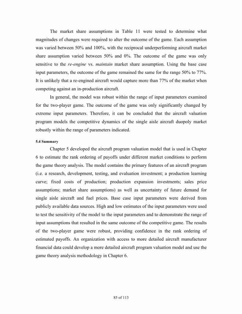
85 of 113
The market share assumptions in Table 11 were tested to determine what
magnitudes of changes were required to alter the outcome of the game. Each assumption
was varied between 50% and 100%, with the reciprocal underperforming aircraft market
share assumption varied between 50% and 0%. The outcome of the game was only
sensitive to the re-engine vs. maintain market share assumption. Using the base case
input parameters, the outcome of the game remained the same for the range 50% to 77%.
It is unlikely that a re-engined aircraft would capture more than 77% of the market when
competing against an in-production aircraft.
In general, the model was robust within the range of input parameters examined
for the two-player game. The outcome of the game was only significantly changed by
extreme input parameters. Therefore, it can be concluded that the aircraft valuation
program models the competitive dynamics of the single aisle aircraft duopoly market
robustly within the range of parameters indicated.
5.4 Summary
Chapter 5 developed the aircraft program valuation model that is used in Chapter
6 to estimate the rank ordering of payoffs under different market conditions to perform
the game theory analysis. The model contains the primary features of an aircraft program
(i.e. a research, development, testing, and evaluation investment; a production learning
curve; fixed costs of production; production expansion investments; sales price
assumptions; market share assumptions) as well as uncertainty of future demand for
single aisle aircraft and fuel prices. Base case input parameters were derived from
publicly available data sources. High and low estimates of the input parameters were used
to test the sensitivity of the model to the input parameters and to demonstrate the range of
input assumptions that resulted in the same outcome of the competitive game. The results
of the two-player game were robust, providing confidence in the rank ordering of
estimated payoffs. An organization with access to more detailed aircraft manufacturer
financial data could develop a more detailed aircraft program valuation model and use the
game theory analysis methodology in Chapter 6.

86 of 113
CHAPTER 6
6.0 Game Theory Analysis of the Incentives to Innovate
This chapter introduces a game theory framework of analysis to evaluate which
factors may incentivize single aisle aircraft manufacturers to innovate. Manufacturers and
policy-makers can apply the methodology developed here to improve the objective
analysis of product line decisions and emission reduction policies. The aircraft program
valuation model developed in Chapter 5 is used to estimate the payoffs for several static
and dynamic games under different market scenarios. The static games demonstrate how
various factors are likely to affect the outcome of the competitive game while the
dynamic games give insight into the timing of the development of a new aircraft. The
market scenarios tested were: (i) expectation of low fuel prices, (ii) technology forcing
regulations, (iii) manufacturer subsidies, (iv) expectation of high fuel prices, and (v) new
market entrants. First, a brief introduction to game theory is provided.
6.1 Game Theory
Von Neumann and Morgenstern founded the field of game theory in their seminal
1944 book Theory of Games and Economic Behavior. They were in search of a more
effective way of solving certain kinds of economic problems to account for the presence
of others who are making decisions in accordance with their own best wishes (Davis,
1997). In a competitive environment, game theory provides a framework to analyze the
impacts of competition on players’ decisions. Lindstädt and Müller (2009) describe their
use of game theory as a technique to support managerial decisions by developing a range
of outcomes based on decisions by reasonable actors. In a complex world, there must be a
balance between simplifying a problem to make it manageable and retaining enough
complexity to make it relevant. Managers must be aware of the assumptions that were
used to find a solution, as the final outcome is sensitive to the initial conditions.

87 of 113
A game has two or more players, each of whom are assumed to be rationally self-
interested, seeking the highest possible benefit. The key requirements of a game theory
analysis are determining: (1) the structure of the game, and (2) the payoffs. The structure
of the game is the set of strategies available to each player. A strategy is a player’s
complete plan of action at each decision point to the end of the game. The payoffs
available to each player for each strategy, given the other players’ strategies, represent
the benefit the player achieves at the completion of the game. Payoffs can be monetary or
non-monetary. Time, utility, and happiness may be equally or more important than
money. The payoff to use in the game theory analysis is dependent on the assumed
objective function of the players. The structure of the single aisle aircraft manufacturer’s
games analyzed in this chapter was introduced in Chapter 4 while the aircraft program
valuation model developed in Chapter 5 is used to estimate the payoffs.
This analysis uses normal form games to determine the outcomes. A normal form
game displays the strategies for each player, and the payoffs for each combination of the
players’ strategies, in a matrix where the first number in each cell represents the payoff
for Player A given Player B’s strategy, and the second number in each cell represents the
payoff for Player B, given Player A’s strategy. The maximum number of players in the
games analyzed in this chapter are three, but the constraints of a two dimensional page do
not limit the possible number of players in a game theory analysis.
The outcome of the game is determined by finding the Nash equilibrium. A Nash
equilibrium is the predicted strategy for each player that is the best response to the
predicted strategy of all other players (Gibbons, 1992). A dominant strategy has a higher
payoff than all other strategies for a player, no matter what strategy the other player
selects. In each normal form game presented, the underlined payoffs represent the best
strategy for each player, assuming the other players’ strategy selection. For example, in
Table 17: assuming Player B selects the maintain strategy, the set of possible payoffs for
Player A is [43, 34, 29]. As 43 is the highest payoff, it is underlined to indicate that if
Player B chooses to maintain, the best strategy for Player A is to maintain. To determine
the Nash equilibrium, this logic is repeated for each strategy, for each player. The cell
with payoffs for both players underlined represents the Nash equilibrium as neither player
can choose a better strategy, given the actions of the other player.

88 of 113
Mixed strategy Nash equilibriums occur when a probability is assigned to each of
the competitors’ strategies. Mixed strategies can be used to determine unique Nash
equilibriums when multiple pure strategy equilibriums exist. Mixed strategies are not
incorporated into this analysis, although they provide an interesting extension of
complexity that could be incorporated into future work.
The normal form games examined are solved simultaneously. Players are
assumed to make their decisions within the same time frame. Although one player may
announce their decision before the other, this action could simply indicate a signaling
game in which one player attempts to impact the other player’s decision. The decision to
proceed with an aircraft program is only truly made when significant disincentives to
reversing the decision exist (such as a substantial order backlog for the new aircraft, or
significant sunk costs in design and engineering work exist).
It is assumed that all players have perfect information enabling competitors to
determine each other’s payoffs for each strategy set. This assumption may not be entirely
true in reality, but the aircraft program valuation sensitivity analysis performed in
Chapter 5 demonstrates that the outcome of the two-player game is primarily sensitive to
the learning curve assumptions. Therefore, as long as competing players’ learning curves
are similar in nature, it is reasonable to assume that they are able to estimate competitors’
payoffs within the margin of error required to maintain the same outcome of the game.
This is a conceptual analysis in which players are assumed to be symmetric,
except for the difference in re-engining investment required by Player A and Player B (as
discussed in Chapters 4 and 5). Labeled A, B, and C, the players in the games presented
are not meant to reflect real world manufacturers. It is assumed that Players A and B are
incumbent manufacturers that have existing single aisle aircraft product lines, while
Player C is a new competitor with the strategy set [Enter, Don’t Enter].
Nine games are examined, as summarized in Table 16:

89 of 113
Table 16. Overview of Games Played Expectation(Fuel Price) indicates the low fuel price (-) or increasing fuel price (+) scenarios.
Games Players Type E(Fuel Price) 2 3 Static Dynamic - +
1) Expectation of Low Fuel Prices x x x 2) Technology Forcing Regulations x x x 3) Manufacturer Subsidies x x x 4) Expectation of High Fuel Prices x x x 5) New Entrant, -25% Fuel Intensity x x x 6) New Entrant, -15% Fuel Intensity x x x 7) Two-Player Dynamic Game x x x 8) New Entrant Dynamic Game, -25% x x x 9) New Entrant Dynamic Game, -15% x x x
Game 1 is the base case against which the other games are compared to
understand how the scenario examined impacts the outcome of the game. Complexity is
built up with each game, providing an understanding of how different factors change the
expected outcome of the game. Two- and three-player games were analyzed to
understand the impact of new competition on the current duopoly market. Static and
dynamic games were used to show how long-term product line strategies might impact
decisions made in the present. The expectation of future fuel prices had important
impacts on the outcome of the games investigated. The first three games were played
under the expectation of low fuel prices, while the remaining games assumed increasing
fuel prices.
6.2 Two-Player Static Games
Game 1: Expectation of Low Fuel Prices
Figure 47. Game 1 Expectation of Low Fuel Prices Decision Timeline
Under the expectation of low fuel prices, incumbent manufacturers are not able to
increase the sale price of a new aircraft as fuel cost savings are negligible over the course
of the aircraft’s life. The incentive to develop a new aircraft is to gain market share from
a competitor or to raise entrance barriers to protect against new entrants. Table 17 shows

90 of 113
that the status quo is the competitive equilibrium. Both incumbents maintain their current
aircraft, reaping large profits while splitting the market. The development of a new
aircraft is strictly dominated for both players. This scenario provides a baseline against
which scenarios explored in the next sections can be compared to understand their
impacts. Table 17. Game 1 Low Fuel Prices E(NPV) billions 2010 US$. (Player <A>, <B>)
Player B
Maintain Re-engine New
Maintain 43, 43 32, 33 18, 29
Re-engine 34, 32 25, 24 17, 16
Play
er A
New 29, 17 16, 15 7, 7
Game 2: Technology Forcing Regulations
Figure 48. Game 2 Technology Forcing Regulations Decision Timeline
If low fuel prices are expected, a technology forcing regulation could be
implemented to obsolete existing aircraft product lines, forcing manufacturers to re-
engine or develop a new aircraft. Rutherford and Zeinali (2009) point out that if the
standard applied to new aircraft types, grandfathering in existing production lines, the
introduction of new aircraft designs may be delayed to avoid triggering the standard. It is
assumed here that the regulation would force manufacturers to either exit the market, re-
engine, or develop a new aircraft within a five-year time frame (i.e. one stage in the
valuation model). Exiting the market would be preceded by a phase-in period in which
incumbent manufacturers sell their current product lines while replacements are
developed, resulting in a positive exit payoff, as shown in Table 18. The predicted
equilibrium is for manufacturers to harvest their existing product lines while making the
minimum investment to meet the regulation by re-engining. Incumbent manufacturers

91 of 113
would not have an incentive to make the larger investment required to develop a new
aircraft in the near-term.
Table 18. Game 2 Technology Forcing Regulations
Player B
Exit Re-engine New
Exit 11, 11 11, 57 11, 39
Re-engine 59, 11 25, 24 17, 16 Pl
ayer
A
New 39, 11 16, 15 7, 7
In this scenario, the manufacturers’ payoffs are reduced by 40% from the low fuel
price scenario. This suggests that manufacturers have a significant incentive to lobby
against technology forcing regulations that would obsolete their existing product lines
unless the regulations yield additional benefits for the incumbents. Games 5 and 6
introduce a new entrant to the market. Increased competition may further erode
manufacturer payoffs as the market is split between three competitors instead of two.
Although technology-forcing regulations may force incumbents to move, they have the
additional effect of raising market entrance barriers by requiring higher technology levels
that favor entrenched incumbent manufacturers. Therefore, under the threat of a new
market entrant, incumbent manufacturers may use their political power to seek
regulations that raise entrance barriers, creating a situation of regulatory capture in which
government action protects incumbents at the expense of new competition (Stigler,
1971).
Game 3: Manufacturer Subsidies
Figure 49. Game 3 Manufacturer Subsidies Decision Timeline
Aircraft manufacturers have traditionally received substantial direct and indirect
subsidies. The rationale by governments has been to support their national champion to
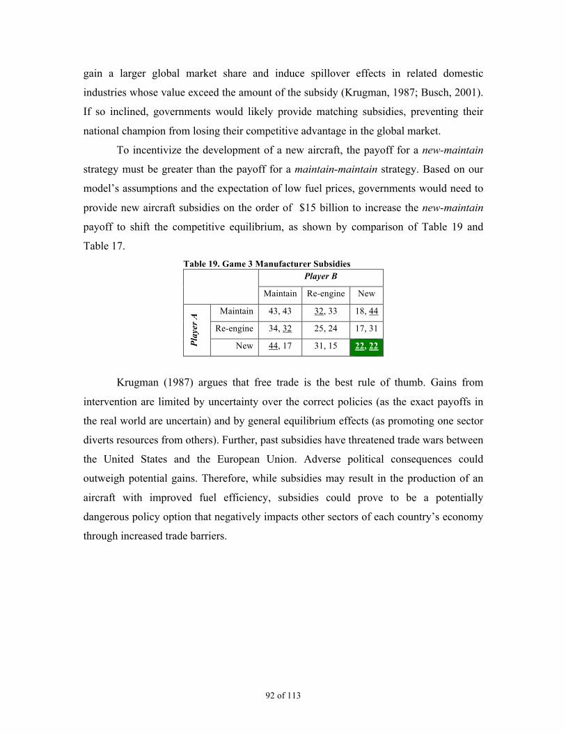
92 of 113
gain a larger global market share and induce spillover effects in related domestic
industries whose value exceed the amount of the subsidy (Krugman, 1987; Busch, 2001).
If so inclined, governments would likely provide matching subsidies, preventing their
national champion from losing their competitive advantage in the global market.
To incentivize the development of a new aircraft, the payoff for a new-maintain
strategy must be greater than the payoff for a maintain-maintain strategy. Based on our
model’s assumptions and the expectation of low fuel prices, governments would need to
provide new aircraft subsidies on the order of $15 billion to increase the new-maintain
payoff to shift the competitive equilibrium, as shown by comparison of Table 19 and
Table 17. Table 19. Game 3 Manufacturer Subsidies
Player B
Maintain Re-engine New
Maintain 43, 43 32, 33 18, 44
Re-engine 34, 32 25, 24 17, 31
Play
er A
New 44, 17 31, 15 22, 22
Krugman (1987) argues that free trade is the best rule of thumb. Gains from
intervention are limited by uncertainty over the correct policies (as the exact payoffs in
the real world are uncertain) and by general equilibrium effects (as promoting one sector
diverts resources from others). Further, past subsidies have threatened trade wars between
the United States and the European Union. Adverse political consequences could
outweigh potential gains. Therefore, while subsidies may result in the production of an
aircraft with improved fuel efficiency, subsidies could prove to be a potentially
dangerous policy option that negatively impacts other sectors of each country’s economy
through increased trade barriers.

93 of 113
Game 4: Expectation of Increasing Fuel Prices
Figure 50. Game 4 Expectation of Increasing Fuel Prices Decision Timeline
Under the expectation of increasing effective fuel prices (due to market forces
and/or carbon pricing policies), it is assumed that manufacturers are able to increase the
sale price of new aircraft that reduce fuel burn. The expected lifecycle fuel cost savings is
split between the airline and manufacturer, as described in Chapter 5. Therefore, a new
aircraft program yields increased revenue for the manufacturer, but requires a large
capital investment and significant demand to reduce unit costs by working down the
production learning curve. If demand does not develop as expected, this can be a risky
endeavour. Table 20 demonstrates that the increased revenue from a higher sale price
provides the incentive required to shift the equilibrium to a new aircraft for both players.
Table 20. Game 4 Increasing Fuel Prices
Player B
Maintain Re-engine New
Maintain 43, 43 32, 48 17, 60
Re-engine 50, 32 37, 35 24, 39
Play
er A
New 60, 17 39, 23 25, 25
This game is a Prisoner’s Dilemma - each player would be better off maintaining
their current aircraft, but each has an incentive to deviate, resulting in reduced payoffs for
both. Implicit or explicit collusion between the incumbents could result in both
manufacturers maintaining their current aircraft, receiving the highest combined payoffs,
but testing airlines’ and governments’ willingness to accept competitive distortions.
Collusion would result in technology levels stagnating, providing an opportunity for new
entrants to develop a competitive aircraft that could take market share away from the
incumbents, as discussed in the next section. In fact, the manufacturer subsidies

94 of 113
examined in Game 3 resulted in a Prisoner’s Dilemma as well, but the dilemma was
induced by government intervention. Competitive forces induce the dilemma in Game 4.
This scenario assumes a ~20% increase in new aircraft sale prices, resulting in a
significant transfer of capital from airlines and leasing companies to manufacturers.
Increased capital requirements would be offset by reduced airline operating costs over
time, but it is uncertain whether additional capital is available for the airlines. The airline
industry is highly competitive and has historically had limited profits.
Undercapitalization of airlines could stall the introduction of new aircraft models by
manufacturers.
For the remainder of the games examined in this paper, the expectation of
increasing fuel costs using the base case values shown in Table 14 were used to calculate
the expected aircraft sale price increase over the base price.
6.3 Three-Player Static Games
Figure 51. New Entrant Extended Form Game
With a new entrant, the game changes from a single move to two moves, as
shown in Figure 51. In the first move, Player C decides whether or not to enter the
market. In the second move, the incumbent manufacturers simultaneously choose their
best response to the new entrant’s strategy. To deter Player C from entering the market,
the incumbents could send credible threats of developing a new aircraft that is superior to
the new entrant’s. Further, the new entrant could send a threat forcing the incumbents to
decide their optimal strategy given their perceived probability of a new competitor
entering the market. For this analysis, it is assumed that Player A and B decide their
optimal strategy given Player C’s decision to enter the market. Given this outcome,
Player C would decide whether or not to enter. Therefore, if Player C expected a negative
E(NPV) given Player A and B’s expected response to the new entrant, Player C would
decide to not enter the market, returning the game to the two-player games discussed in

95 of 113
Games 1 to 4. Games 5 and 6 demonstrate that the performance of the new entrant’s
aircraft impacts the outcome of the game. An aircraft with superior performance would
capture a greater market share, reducing the incumbents’ payoffs further.
Game 5: New Entrant, -25% Fuel Intensity
Figure 52. Game 5 New Entrant, -25% Fuel Intensity Decision Timeline
If the new entrant’s aircraft has superior performance to the incumbents’, the
incumbents would expect to lose a significant number of sales, providing them with an
incentive to develop a new aircraft. Assuming that sale prices are increased to reflect
lifecycle fuel cost savings under the increasing effective fuel price scenario (as in Game
4) and that the new entrant produces a new aircraft that meets the performance of the
incumbent’s new aircraft option (i.e. a 25% fuel burn improvement), Table 21 shows that
an equilibrium may exist in which one incumbent chooses to maintain while the other
decides to re-engine. Although this equilibrium is sensitive to the input parameters in the
aircraft program valuation model, the greater investment required by Player B to re-
engine results in an off-symmetric equilibrium. The superior performance of the new
entrant’s aircraft captures a significant market share while Player A attempts to maintain
market share by re-engining. Player B’s optimal strategy is to avoid the investment and
maintain its current aircraft. Once the competitors’ new and re-engined aircraft enter
service in stage 2, Player B suffers from a greatly reduced market share, but continues to
make small profits due to its unit production cost advantage while harvesting its existing
product line. The new entrant has a positive expected net present value in each possible
outcome, except if both of the incumbents develop a new aircraft. This result suggests
that there may be rents available in the single aisle market, providing an incentive for
increased competition if new entrants are able to overcome the significant entrance
barriers to develop an aircraft that can compete with the incumbents’ new aircraft option.

96 of 113
Table 21. Game 5 New Entrant, -25% Fuel Intensity E(NPV) billions 2010 US$. (Player <A>, <B>, <C>)
Player B Maintain Re-engine New
Maintain 17.1, 17.1, 29
17.1, 16, 20
17.1, 17.3, 5
Re-engine 17.5, 17.1, 20
17.5, 16, 11
17.5, 13, 1
Play
er A
New 17.3, 17.1,
5 13, 16,
1 9.5, 9.5,
-2.4
Game 6: New Entrant, -15% Fuel Intensity
Figure 53. Game 6 New Entrant, -15% Fuel Intensity Decision Timeline
Due to limited design and production experience, a new entrant may not be able
to match the incumbents’ new aircraft option performance. In Game 6, it is assumed that
the new entrant is only able to develop an aircraft that matches the performance of the
incumbents’ re-engined aircraft (i.e. a 15% fuel burn improvement). A different off-
symmetric equilibrium is shown in Table 22. Player B develops a new aircraft to
maintain a 50% market share while Players A and C split the remaining market by
offering an aircraft with an inferior performance to Player B’s.
Table 22. Game 6 New Entrant, -15% Fuel Intensity
Player B Maintain Re-engine New
Maintain 24.6, 24.6, 11
20.8, 27.4, 3
17.1, 28.8, -5
Re-engine 29, 20.8, 3
23.7, 22.2, -2
17.5, 24.2, -8
Play
er A
New 28.8, 17.1, -5
24.2, 16.0, -8
15.1, 15.1, -11
The new entrant only receives a positive payoff if neither incumbent develops a
new aircraft. This result suggests that a profit-maximizing firm would decide to not enter

97 of 113
the market. Therefore, incumbent manufacturers may not be concerned with new entrants
unless there is a threat that they could match or exceed the performance of the
incumbents’ new aircraft option. But, if a new entrant has government support, it may be
profitable to enter the market. Further, if the new entrant has a different objective
function than the incumbents’, other factors may make it beneficial to enter the market,
such as spillover effects to other sectors of the economy, national pride, and military
capabilities. Therefore, when determining the probability of a new competitor entering
the market, additional factors must be taken into account.
The three-player static games have shown how differences in the investment
required by incumbent players may result in off-symmetric game equilibriums as well as
how new competition in addition to increased expected fuel prices may shift the
competitive equilibrium from the duopoly equilibrium in Game 1.
6.4 Two-Player Dynamic Game
If manufacturers consider how their decisions in the present impact future product
line decisions, the game can be modeled dynamically where the evolution of demand and
fuel prices impacts the equilibrium strategy set. Committing to a re-engined or new
aircraft locks into a technology level for 10 or more years, requires an investment, and
can be risky. Delaying the decision provides more flexibility for future actions, but gives
competitors an opportunity to develop a superior aircraft. If it is assumed that both
incumbent manufacturers will decide to proceed with a new aircraft by the third stage
(i.e. 2020-24), a dynamic game (as depicted in Figure 54) can be evaluated to understand
the timing of the decision, given the competitive scenarios developed in this section.
Game 7: Two-Player Dynamic Game
Figure 54. Game 7 Two-Player Dynamic Game Decision Timeline

98 of 113
The dynamic game examined has four stages: 2010-14, 2015-19, 2020-24, and
2025-2039. Incumbent manufacturers are able to select the maintain, re-engine, or new
strategies at each of the first two stages, but are forced to choose new in the third. It is
assumed that the re-engine strategy is a stopgap until a new aircraft enters into service ten
years after the re-engined aircraft. This creates a fourth strategy for the incumbents
named delay. For the delay strategy, the decision to develop a new aircraft is delayed five
years to the second stage, for entry into service in the third stage (2020-2024).
The payoff for the new strategy was determined for the fourth stage, based on the
expected demand and fuel prices. Increased fuel costs enabled manufacturers to increase
the sale price of the new or re-engined aircraft while the existing aircraft sale price was
assumed to hold constant in real dollar terms. Technology levels were assumed to
improve at the rates shown in Figure 35. Therefore, delaying the decision enabled a
superior aircraft to be developed that yielded a higher sale price, assuming the
expectation of future fuel prices increased or remained constant. Backwards induction
down each possible decision path, with each possible fuel and demand scenario, was used
to determine the expected payoffs in present value terms in the normal form game shown
in Table 23. The dynamic game demonstrates that delaying the development of a new
aircraft to take advantage of improved technology levels and increased sale prices may be
the incumbents’ optimal strategy.
Table 23. Game 7 Two-Player Dynamic Game
Player B Maintain Re-engine New Delay
Maintain 38, 38 30, 39 35, 34 29, 48
Re-engine 40, 30 31, 30 28, 34 31, 37
New 34, 35 34, 26 27, 27 33, 31
Play
er A
Delay 48, 29 37, 30 31, 33 35, 35
The two-player dynamic game was repeated for each combination of the high/low
fuel price and demand scenarios in Table 14. Higher fuel prices raise the value of fuel
burn reduction technologies, enabling manufacturers to increase the sale price of new and
re-engined aircraft, while high demand enables manufacturers to work down the
production learning curve more rapidly and spread the fixed costs of development across

99 of 113
more aircraft. The low states have the opposite effects. It was found that varying demand
did not alter the outcomes of the dynamic game, whereas the low fuel price scenarios
resulted in both players selecting the maintain strategy. Therefore, as in the static game,
the expectation of higher fuel costs drives manufacturers to develop a new aircraft. This
is a result of the aircraft program valuation model’s greater sensitivity to price than
demand, as shown in Figure 46. All dynamic game results displayed were found using the
expectation of increasing fuel costs.
6.5 Three-Player Dynamic Games
Game 8: New Entrant Dynamic Game, -25% Fuel Intensity
Figure 55. Game 8 New Entrant Dynamic Game, -25% Fuel Intensity Decision Timeline
The dynamic game was played with a new market entrant in the 2015-19 time
frame. This analysis enabled the understanding of how new competition – or the credible
threat of new competition – may change the game. As in Games 5 and 6, the level of
performance of the new entrant’s aircraft impacted the outcome of the game. A new
entrant’s aircraft with the same performance as the incumbents’ new option would take
significant market share unless the incumbents’ decide to move. A new entrant’s aircraft
that has the same performance as the incumbents’ re-engined aircraft would capture less
market share.
Table 24 shows that there are two potential pure strategy equilibriums. While the
incumbents may find it most profitable to harvest their existing product lines, there is an
incentive for one incumbent to develop a new aircraft, but not both. The incumbents play
a waiting game, with the first one to move taking the risk of developing a new aircraft
along with a higher expected payoff, while the other stands pat with the less risky
maintain strategy. To determine which manufacturer is likely to move first would require
information regarding the incumbent manufacturer’s assessment of the probability of a

100 of 113
new entrant and the new entrant’s aircraft performance. The manufacturer that believes it
is more likely that a new competitor will enter the market with a competitive aircraft will
be the first to move, resulting in the late mover delaying the introduction of their new
aircraft until the fourth stage (2025-29). The payoffs for the first mover to select the new
or delay strategy are very close, with payoffs that are sensitive to the assumptions of the
aircraft program valuation model. Therefore, the timing of the first incumbent’s new
aircraft entry into service may be either the second (2015-19) or third stage (2020-24).
Table 24. Game 8 New Entrant 2015 Dynamic Game, -25% Fuel Intensity Player B Maintain Re-engine New Delay
Maintain 16.7, 16.7, 20.6
16.7, 13.7, 13.9
16.7, 19.7, 2.6
16.7, 19.9, 11.5
Re-engine 15.2, 16.7, 13.9
15.2, 13.7, 7.5
15.2, 16.4, -0.4
15.2, 18.3, 6.8
New 19.7, 16.7, 2.7
16.4, 13.7, -0.4
11.9, 11.9, 0.7
14.8, 15.0, 3.6 Pl
ayer
A
Delay 19.9, 16.7, 11.5
18.3, 13.7, 6.8
15.0, 14.8, 3.6
15.0, 15.0, 10.3
Game 9: New Entrant Dynamic Game, -15% Fuel Intensity
Figure 56. Game 9 New Entrant Dynamic Game, -15% Fuel Intensity Decision Timeline
If a new entrant is expected to develop an aircraft that has the same performance
as the incumbents’ re-engined aircraft, the incumbents have an incentive to develop a
new aircraft, as shown in Table 25. The Nash equilibrium is predicted to be the case were
either Player A or B enters a new aircraft into service in 2015-19 while the other delays
until 2020-24. Player C gains less market share than required to have a positive E(NPV),
suggesting an early move by one of the incumbents could prevent the new competitor
from entering the market. The incumbent that delays entry into service of a new aircraft

101 of 113
temporarily loses market share while it produces an aircraft inferior to the new entrant
and the other incumbent, regaining market share in the third stage (2020-24) when it
introduces a new, superior aircraft. If both incumbents delay the entry into service of a
new aircraft, the new entrant is able to capture significant market share in the short term,
increasing its payoff, and the likelihood of entry.
Table 25. Game 9 New Entrant 2015 Dynamic Game, -15% Fuel Intensity Player B Maintain Re-engine New Delay
Maintain 22.8, 22.8, 6.1
20.1, 21.9, -0.2
17.5, 28.9, -6.0
20.4, 27.9, 0.2
Re-engine 23.4, 20.1, -0.2
20.0, 18.5, -4.2
16.0, 25.6, -8.6
19.7, 24.7, -4.5
New 28.9, 17.5, -6.0
25.6, 14.5, -8.6
19.7, 19.7, -12.3
24.7, 20.7, -10.1 Pl
ayer
A
Delay 27.8, 20.4, 0.2
24.7, 18.2, -4.5
20.7, 24.7, -10.1
23.6, 23.7, -4.4
The three-player dynamic games are sensitive to the aircraft program valuation
model and market share assumptions, but are used here to demonstrate how the credible
threat of new competition may lead incumbent manufacturers to select different strategies
depending on their own risk tolerance and assessment of the threat of new competition.
6.6 Summary
The static Games 1 to 6 demonstrated the impact of different scenarios on the
single-aisle aircraft manufacturer’s competitive game. Dynamic decision-based analysis
was introduced to combine multiple factors in Games 7 to 9, demonstrating how a game
theory analysis of the single aisle aircraft market segment may be used to determine the
optimal timing of manufacturer’s strategies. Table 26 summarizes the games discussed,
showing that while subsidies or expected increasing fuel prices may incentivize the
development of new aircraft, consideration of longer-term strategies in the dynamic game
may provide incentives for manufacturers to delay the entry of a new aircraft. This may
result in superior performing aircraft that enter into service in the next decade, at the cost
of increased carbon emissions in the near-term. Kar (2010) showed that early entry into
service of available technology (as opposed to delaying entry for more advanced
technologies) has greater potential to improve fleet fuel-burn performance due to the

102 of 113
dynamics of fleet turnover. Therefore, public policies may be required to incentivize the
development of new aircraft. Table 26. Summary of Game Equilibriums Player B Maintain Re-engine New Delay
Maintain (1) Low Fuel prices (8) Dynamic Game (New Entrant, -25%)
Re-engine (5) New Entrant, -25% Performance
(2) Technology Forcing Regulations
(6) New Entrant, -15% Performance
New (3) Subsidies (4) High Fuel Prices
(9) Dynamic Game (New Entrant, -15%) Pl
ayer
A
Delay (8) Dynamic Game (New Entrant, -25%) (9) Dynamic Game
(New Entrant, -15%) (7) Dynamic Game (2-player)
Different assumptions in the model may lead to different outcomes. For example,
Games 5 and 6 (the static, three-player games) were sensitive to the reduced investment
required by Player A to re-engine. Further, the dynamic games were sensitive to the
expectation that fuel prices will increase. If fuel prices were to drop, the sale price of a
new aircraft with large fuel burn improvements is assumed to decrease, reducing the
incentives to develop a new aircraft. This analysis assumed that all players are rational,
risk-neutral, profit-maximizing firms. Payoffs for firms with different risk tolerances
would be altered, potentially leading to different off-symmetric equilibriums not explored
in this analysis. New entrants to the market from China and Russia may have alternative
objective functions. Other manufacturers may attempt to maximize market share,
minimize costs, or maximize revenues. Softer factors, such as national pride or technical
curiosity, may lead players to make seemingly irrational decisions when evaluated in
profit maximizing terms. Therefore, although this analysis has demonstrated how a
variety of factors and policies may impact the competitive game, it is important for
managers and policy makers to understand the assumptions and the limitations of the
game theory analysis.

103 of 113
CHAPTER 7
7.0 Conclusions
Effective fuel cost increases due to crude oil market prices and environmental
charges may result in air service reductions that have negative economic and social
impacts. The 2004-08 fuel price surge was used as a historical case study to further
understanding of the short- and medium-term impacts of effective fuel cost increase on
the US air transportation system. It was found that non-hub airports serving small
communities lost 12% of connections, compared to a system-wide average loss of 2.8%.
Increased effective fuel costs will provide incentives for airlines to improve fleet fuel
efficiency, reducing the environmental impacts of aviation, but may cause an uneven
distribution of social and economic impacts if small communities suffer greater loss of
mobility. Government action may be required to determine acceptable levels of access as
the system transitions to higher fuel costs.
One long-term hedge against increasing effective fuel costs is efficiency
improvements. Aircraft fuel intensity has historically decreased at a rate of 1.2%-2.2%
per year, but fleet fuel intensity improvements have stalled during the past decade. To
improve aviation’s fuel efficiency new single aisle aircraft with higher technology levels
will be required. Competition is an important factor to consider when designing policies
to reduce aviation’s environmental impacts.
This report outlined a framework of analysis for competition in the single-aisle
aircraft market segment. Using an aircraft program valuation model and a game theoretic
approach, the impacts of market changes on manufacturers’ decisions to maintain, re-
engine, or develop new aircraft was investigated. It was found that subsidies and higher
fuel prices should provide sufficient incentives for incumbent manufacturers to develop
new aircraft, but may lead to Prisoner’s dilemmas in which manufacturers would be
better off not moving from the status quo. New competition in the market segment is
likely to trigger innovation as incumbent manufacturers attempt to produce more efficient

104 of 113
aircraft that maintain sales in a market with increased competition. Interestingly, it was
found that a new entrant’s aircraft that offers a fuel efficiency improvement on the order
of 15% may incentivize the incumbent manufacturers to develop a new aircraft while a
new entrant with a 25% fuel burn improvement may cause incumbents to select a less
risky strategy. Dynamic games demonstrated that the incumbents’ optimal strategies
might be to delay the entry of new single aisle aircraft until 2020-24. As political pressure
mounts to take action on climate change and airlines search for ways to reduce operating
costs in the face of rising effective fuel costs, delaying may not be acceptable. This
situation could result in government intervention to incentivize the development of new
aircraft.
A number of further complexities could be explored using the framework
developed in this report. It was assumed that competitors act with perfect information.
Imperfect information would cast doubt on the technical capabilities of competitors’
aircraft(s) as well as financial payoffs. Incumbent manufacturers could collude either
implicitly or explicitly to select the strategy that yields the highest total payoff with least
risk. The riskiness of new aircraft programs was not incorporated into this analysis. Risk-
averse or risk-seeking players may change the outcome of the games or result in unique
Nash equilibriums in the three-player dynamic games examined. Further, it was assumed
that all manufacturers have the same objective function – to maximize expected net
present value of a program. But aircraft manufacturing has spill over effects that impact
other sectors of a nation’s economy, providing incentives for governments to subsidize
new aircraft programs that may otherwise not be profit maximizing.
This work is an initial step in using game theory to understand the impacts of
competition, market conditions, and technological progress on large commercial aircraft
manufacturer decisions. A number of simplifying assumptions have been made in the
models presented to facilitate the analysis of a problem that quickly scales in complexity.
To tackle this problem in a more holistic manner, a multidisciplinary approach should be
implemented in which the technical and financial implications of strategic options are
integrated into the decision making process. The question of what level of performance to
design into the next generation aircraft has a continuous solution set, not the three-
pronged strategy set used in this work. The technical risk of increasing performance of a

105 of 113
new aircraft impacts the financial risk of the program, while external market conditions
outside of the control of managers will ultimately determine the success of a new
program. Therefore, manufacturers and policy makers will require more complex and
integrated tools to understand the implications of their decisions and to tackle aviation’s
environmental challenges.
The application of game theory to management problems is still a nascent field.
Game theory provides a simple, yet powerful tool to insert objective, competitive analysis
into the decision making process. The decision analysis methodology developed in this
report could be generalized to other applications and fields, such as: semiconductor
fabrication plant investment decisions, automobile product line decisions, and airline fleet
planning decisions. Investment decisions made by agents in a competitive environment
could benefit from a game theory analysis to determine their best strategy, given their
competitors’ likely response.
While aircraft efficiency improvements will reduce airline operating costs, it is
uncertain whether reductions in air service would be mitigated. Further, to meet
environmental goals, efficiency may not be enough. Herring (2006) challenges the idea
that improving the efficiency of energy use will lead to a reduction in energy
consumption. Energy efficiency lowers the implicit price of energy, potentially leading to
greater use. As a greater share of the world’s population gains access to affordable air
transportation in developing countries, aviation’s environmental externalities will
continue to grow. To face the world’s climate change challenge without limiting the
economic enabling effects of air transportation by suppressing demand, aircraft
technology will need to be improved. The incentives for manufacturers to stand still will
need to be overcome.

106 of 113
8.0 References
Airbus (2009). Global Market Fortecast 2009-2028. Cited October 12, 2010. URL: http://www.airbus.com/company/market/gmf2009/
Airbus (2010a). Airbus offers new fuel saving engine options for A320 Family. Cited December 27, 2010. URL: http://www.airbus.com/en/presscentre/pressreleases/press-release/detail/airbus-offers-new-fuel-saving-engine-options-for-a320-family/news-browse/2/news-period/1293439893/
Airbus (2010b). Orders and Deliveries. Cited October 30, 2010. URL:
http://www.airbus.com/en/corporate/orders-and-deliveries/
Air Transport Association (ATA) (2010a). ATA Monthly Jet Fuel Cost and Consumption Report. Retrieved June 18, 2010, http://www.airlines.org/Energy/FuelCost/Pages/MonthlyJetFuelCostandConsumptionReport.aspx
Air Transport Association (ATA) (2010b). Quarterly Cost Index: U.S. Passenger Airlines. Retrieved June 18, 2010, from http://www.airlines.org/Economics/DataAnalysis/Pages/QuarterlyCostIndex.aspx
American Institute of Aeronautics and Astronautics (AIAA) (2010). Inside Aerospace: An International Forum for Aviation and Space Leaders: Report of Discussion and Recommendation.
Babikian, Raffi, Stephen P. Lukachko, Ian A. Waitz (2002). The historical fuel efficiency characteristics of regional aircraft from technological, operational, and cost perspectives. Journal of Air Transport Management 8, 389–400.
Bediér, Christophe, Maxence Vancauwenberghe, and Wolf van Sintern (2008). The growing role of emerging markets in aerospace. The McKinsey Quarterly. Cited August 27, 2010. URL: https://www.mckinseyquarterly.com/home.aspx
Benkard, C. Lanier (2000). Learning and Forgetting: The Dynamics of Aircraft Production. The American Economic Review, Vol. 90, No. 4, 1034-1054.
Benkard, C. Lanier (2004). A Dynamic Analysis of the Market for Wide-Bodied Commercial Aircraft. Review of Economic Studies 71, 581-611. Boeing (2000-2009). Annual Report. Cited March 22, 2011. URL: http://www.boeing.com/companyoffices/financial/quarterly.htm

107 of 113
Boeing (2005). 737 Airplane Characteristics for Airport Planning. D6-58325-6.
Boeing (2010a). Current Market Outlook 2010-2029. Cited October 12, 2010. URL: http://www.boeing.com/commercial/cmo/
Boeing (2010b). Orders and Deliveries. Cited October 30, 2010. URL:
http://active.boeing.com/commercial/orders/index.cfm
Boeing (2010c). Who Has the Newest Single-Aisle Jetliners? Cited October 13, 2010. URL: http://www.boeing.com/commercial/737family/pf/pf_newest.html
Brander, James A. and Barabar J. Spencer (1985). Export Subsidies and International Market Share Rivalry. Journal of International Economics 18.
Brueckner, Jan K., and Anming Zhang (2010). Airline emission charges: Effects on airfares, service quality, and aircraft design. Transportation Research Part B. doi:10.1016/j.trb.2010.02.006
Bureau of Economic Analysis (BEA) (2010, July 30). National Economic Accounts. Cited August 2, 2010. URL: http://www.bea.gov/national/index.htm#gdp
Bureau of Transportation Statistics (BTS) (2009, January 28). Average Third-
Quarter Domestic Air Fares Reach Highest Quarterly Level; Top 100 Airports: Highest Fare in Cincinnati, Lowest Fare at Dallas Love. Cited February 3, 2010. URL: http://www.bts.gov/press_releases/2009/bts005_09/html/bts005_09.html
Bureau of Transportation Statistics (BTS) (2010a). Average Domestic Airline Itinerary Fares By Origin City. Cited June 12, 2010. URL: http://www.transtats.bts.gov/AverageFare/
Bureau of Transportation Statistics (BTS) (2010b). Form 41 T100 and T2. Cited January 27, 2010. URL: http://www.transtats.bts.gov/ Burghouwt, Guillaume (2005). Airline Network Development in Europe and its Implications for Airport Planning. Ph.D. thesis, Faculty of Geosciences, Utrecht University.
Busch, Marc (2001). Trade Warriors: States, Firms, and Strategic-Trade Policy
in high-Technology Competition. Cambridge University Press, Cambridge, UK.
Butler, S. E., & Kiernan, L. J. (1992). Estimating the Regional Economic Significance of Airports. FAA, National Planning Division.
Cento, A. (2009). The Airline Industry: Challenges in the 21st Century. Segrate, Italy: Physica-Verlag Heidelberg.

108 of 113
Chance, Don M. (2007). A Synthesis of Binomial Option Pricing Models for Lognormally Distributed Assets. Louisiana State University, Baton Rouge. Cited February 3, 2011. URL: http://ssrn.com/abstract=969834 Darson, Lauren (2011). Senate Approves FAA Reauthorization Bill, Awaits House Vote. Travel Management. Cited March 29, 2011. URL: http://www.management.travel/news.php?cid=FAA-reauthorization-bill-Senate-approves.Feb-11.23 Davis, Morton D. (1997). Game Theory: A Nontechnical Introduction. Mineola, NY: Dover Publications, Inc.
EADS (2000-2009). Annual Report. Cited March 22, 2011. URL:
http://www.eads.com/eads/int/en/investor-relations/events-reports/annual-report/2010.html
Energy Information Administration (EIA) (2010, May 11). Annual Energy Outlook 2010. Cited June 28, 2010. URL: http://www.eia.doe.gov/oiaf/aeo/
Environmental Protection Agency (EPA) (2009, June). American Clean Energy and Security Act of 2009 - H.R. 2454. Cited July 22, 2010. URL: http://www.epa.gov/climatechange/economics/economicanalyses.html#hr2454
Federal Aviation Administration (FAA) (2008). Report to Congress: National Plan of Integrated Aiport Systems 2009-2013.
Ferreri, Domenico (2003). Marketing and management in the high-technology sector: strategies and tactics in the commercial airplane industry. Praeger: Westport, Conn.
GeoLytics (2000). Census 2000 Demographic Data Products. East Brunswick, NJ, USA.
Gibbons, Robert (1992). Game Theory for Applied Economists. Princeton University Press: Princeton, New Jersey.
Gillen, David W., William G. Morrison, and Christopher Stewart (2008). Air Travel Demand Elasticities: Concepts, Issues and Measurement. Government of Canada, Department of Finance Canada.
Gittell, Jody Hoffer, and Charles O’Reilly (2001). JetBlue Airways: Starting from Scratch. Harvard Business School Case Study, N1-801-354.
Gittell, Jody Hoffer, Andrew von Nordenflycht, Thomas A. Kochan, Robert
McKersie and Greg J. Bamber (2009). “Labor Relations and Human Resource

109 of 113
Management in the Airline Industry.” In P. Belobaba, C. Barnhart, and A. Odoni (Eds.), The Global Airline Industry (275-311). West Sussex: John Wiley & Sons, Ltd.
Goetz, Andrew R., and Christopher J. Sutton (1997). The Geography of Deregulation in the U.S. Airline Industry. Annals of the Association of American Geographers , 87 (2), 238-263.
Google (2009). Google Maps. Cited December 16, 2009. URL: http://maps.google.com/
Government Accountability Office (GAO) (2003). Factors Affecting Efforts to Improve Air Service at Small Community Airports. GAO-03-330.
Government Accountability Office (GAO) (2009). Airline Industry Contraction Due to Volatile Fuel Prices and Falling Demand Affects Airports, Passengers, and Federal Government Revenues. GAO-09-393.
Greitzer, E. M. et. al. (2010). N+3 Aircraft Concept Designs and Trade Studies: Final Report. Massachusetts Institute of Technology.
Herring, Horace (2006). Energy efficiency – a critical view. Energy 31, 10–20.
International Civil Aviation Authority (ICAO) (2010). “ResolutionA37-19:
Consolidated statement of continuing ICAO policies and practices related to environmental protection – Climate change.” Cited December 13, 2010. URL: http://www.icao.int/icao/en/env2010/Index.html International Air Transport Association (IATA) (2010). Fact Sheet: Economic & Social Benefits of Air Transport. Cited February 14, 2011. URL: http://www.iata.org/pressroom/facts_figures/fact_sheets/Pages/economic-social-benefits.aspx
Irwin, Douglas A. and Nina Pavcnik (2004). Airbus versus Boeing revisited: international competition in the aircraft market. Journal of International Economics 64, 223-245.
Ishutkina, M. A., and Hansman, R. J. (2008). Analysis of Interaction between Air Transportation and Economic Activity. AIAA 8th Aviation Technology, Integration, and Operations Conference. Anchorage, Alaska.
Justin, Cedric Y., Elena Garcia, and Dimitri N. Mavris (2010). Aircraft Valuation: A Network Approach to the Evaluation of Aircraft for Fleet Planning and Strategic Decision Making. AIAA 10th Aircraft Technology, Integration, and Operations Conference. September 13-15, 2010. Fort Worth, TX.

110 of 113
Kar, Rahul, Philippe A. Bonnefoy, R. John Hansman, and Sgouris Sgouridis (2009). Dynamics of Implementation of Mitigating Measures to Reduce Commercial Aviation’s Environmental Impacts. 9th AIAA Aviation, Technology, Integration, and Operations (ATIO) Conference. September 21-23, 2009. Hilton Head, SC.
Kar, Rahul (2010). Dynamics of Implementation of Mitigating Measures to Reduce CO2 Emissions from Commercial Aviation. S.M. thesis: Massachusetts Institute of Technology.
Krugman, Paul R. (1987). Is Free Trade Passé? Economic Perspective, Vol 1 Number 22, 131-144.
Lee, D.S., Pitari, G., Grewe, V., Gierens, K., Prenner, J., Petzold, A., et al. (2009). Transport impacts on atmosphere and climate: Aviation. Atmospheric Environment.
Lee, Joosung J., Stephen P. Lukachko, Ian Waitz, and Andreas Schafer (2001). Historical and Future Trends in Aircraft Performance, Cost, and Emissions. Annual Review of Energy and the Environment, 26:167-200.
Lindstädt, Hagen and Jürgen Müller (2009). Making game theory work for
managers. McKinsey Quarterly. Cited January 26, 2011. URL: https://www.mckinseyquarterly.com/Making_game_theory_work_for_managers_2493
Lissys (2009). Piano-X. Cited January 27, 2010. URL: http://www.lissys.demon.co.uk/index2.html
Malina, R., Schwab, M., and Wollersheim, C. (2008). Using a Contingent
Valuation Approach for Evaluating the Benefits of Airports for Regional Economies.
Markish, Jacob (2002). Valuation Techniques for Commercial Aircraft Program Design. S.M. Thesis: Massachusetts Institute of Technology.
Masschusetts et. al. v. Environmental Protection Agency, 05-1120 U.S. (2007).
Mavris, Dimitri and Mark Birney (2002). Formulation of a Stochastic, Physics-Based Strategic Business Decision Making Environment. AIAA 2nd Aircraft Technology, Integration, and Operations Conference. October 1-3, 2002. Los Angeles, CA.
Morrell, Peter and Lynnette Dray (2009). Environmental aspects of fleet turnover, retirement and life cycle. Omega, Cranfield University.
Morris, Joe, Alex Rowbotham, Andy Angus, Mike Mann, and Ian Poll (2009). A Framework for Estimating the Marginal Costs of Environmental Abatement for the Aviation Sector. Omega, Cranfield University.

111 of 113
National Transportation Safety Board (NTSB) (2009, May). Accidents Involving Passenger Fatalities U. S. Airlines (Part 121) 1982 - Present. Cited June 12, 2010. URL: http://www.ntsb.gov/aviation/Paxfatal.htm
Newhouse, John (2007). Boeing versus Airbus: The Inside Story on the Greatest International Competition in Business. New York: A.A. Knopf.
Nolan, James, Pamela Ritchie, and John Rowcroft (2005). Small Market Air
Service and Regional Policy. Journal of Transport Economics and Policy, Vol. 39, Part 3, pp. 363-378.
Office of Aviation Analysis. (2010). Essential Air Service Program. Cited June 16, 2010. URL: http://ostpxweb.dot.gov/aviation/x-50%20role_files/essentialairservice.htm
Pearce, Brian (2009). The case for wider and deeper liberalisation of air transport. International Air Transport Association. Cited February 16, 2011. URL: http://www.iata.org/Documents/economics/Agenda_For_Freedom_Presentation.pdf
Peeters, P.M. and J. Middel, and A. Hoolhorst (2005). Fuel Efficiency of Commercial Aircraft: An Overview of Historical and Future Trends. National Aerospace Laboratory NLR, The Netherlands.
Penner, J.E., D.H.Lister, D.J.Griggs, D.J.Dokken, and M.McFarland (Eds.) (1999). Aviation and the Global Atmosphere. Intergovernmental Panel on Climate Change (IPCC), Cambridge University Press, UK.
Peoples, Ryan E. (2004). Value-Based Multidisciplinary Optimization for Commercial Aircraft Program Design. S.M. Thesis, Massachusetts Institute of Technology.
Raymer, Daniel P. (2006). Aircraft Design: A Conceptual Approach. Washington, D.C.: American Institute of Aeronautics and Astronautics (AIAA).
Rothman, Andrea (December 1, 2010). “Airbus to Offer More Fuel efficient Version of A320 Model Starting in 2016.” Bloomberg. Cited December 1, 2010. URL: http://www.bloomberg.com/news/2010-11-30/eads-said-to-give-airbus-backing-to-upgrade-a320-aircraft-series.html
Rutherford, Daniel and Mazyar Zeinali (2009). Efficiency Trends for New Commercial Jet Aircraft 1960 to 2008. International Council on Clean Transportation (ICCT).
Sgouridis, Sgouris P. (2007). Symbiotic Strategies in Enterprise Ecology: Modeling Commerical Aviation as an Enterprise of Enterprises. Ph.D Thesis: Massachusetts Institute of Technology.

112 of 113
Sgouridis, Sgouris, Philippe A. Bonnefoy, and R. John Hansman (2010). Air
Transportation in a Carbon Constrained World: Long-term Dynamics of Policies and Strategies for Mitigating the Carbon Footprint of Commercial Aviation. Transportation Research Part A.
Steiner, John E. (1982). How Decisions are Made: Major Considerations for Aircraft Programs. AIAA 1982 Wright Brothers Lectureship in Aeronautics. Aircraft Systems and Technology Meeting, August 24, 1982. Seattle, Washington.
Stigler, George J. (1971). The theory of economic regulation. The Bell Journal of Economics and Management Science, Vol. 2, No. 1.
Tam, Ryan and R. John Hansman (2003). An Analysis of the Dynamics of the US Commercial Air Transportation System. S.M. thesis: Massachusetts Institute of Technology.
Tushman, Michael L. and Philip Anderson (1986). Technological Discontinuities and Organizational Environments. Administrative Science Quarterly, Vol. 31, No. 3 (Sep., 1986), pp. 439-465.

113 of 113
APPENDIX
9.0 Airline Classification
Although it is expected that carriers within the same classification vary
significantly in their businesses, markets, and operations, airlines were classified to
simplify the presentation of data. The following categories were used to group airlines
with similar business models, based on common practices found in the literature and the
author’s discretion. The top two US airlines in each category, by July 2007 available seat
miles (ASM), are listed:
• Network Legacy Carrier (NLC) – airlines that flew interstate routes prior to
deregulation in 1978, have international operations, and are certified under Part
121 of Title 14 of the Code of Federal Regulations, including American Airlines
and United Air Lines.
• Low Cost Carrier (LCC) – airlines that have a stated low fare business model,
and are certified under Part 121 of Title 14 of the Code of Federal Regulations,
including Southwest Airlines and JetBlue Airways.
• Regional – feeder, charter, and commuter airlines that fly aircraft less than 100
seats, and are certified under Part 121 of Title 14 of the Code of Federal
Regulations, including Skywest Airlines and Expressjet Airlines.
• Commuter – commuter and on demand airlines that are certified under Part 135
of Title 14 of the Code of Federal Regulations, including Hageland Aviation
Service and Boston-Maine Airways.