Games of sexual selection - Centre de Recherches · PDF file · 2013-11-20Games of sexual selection: static and dynamic aspects Pierre Bernhard & Fred´ eric Hamelin ... (1975):The

Games of sexual selection:static and dynamic aspects

Pierre Bernhard & Frederic Hamelin

BIOCORE teamINRIA-Sophia Antipolis-Mediterranee, France

Institut de Genetique, Environnement et Protection des Plantes,Agrocampus Ouest, INRA/Universite de Rennes 1, France

Workshop “Biodiversity and Environment:a viability and dynamic games perspective”

Montreal, November 4 – 8, 20131

Context

Handicap paradox: In many species, male secondary sexual charactersthat attract females are a viability handicap for the male. The more handi-capped, the more attractive the male !

Fisher (1915) Lande (1981), “runaway” mechanism: a dynamic divergence.

Zahavi’s handicap principle (1975): The character considered signals themale’s “quality”. If a signal is not costly, it can be cheated, and hence is notcredible.

Grafen’s formalization Grafen (1990) offers a mathematical formulation ofZahavi’s principle. We shall develop two models very similar to Grafen’s,but more explicit. We offer an explanation, and a remedy, to an undesirablefeature of Grafen’s model. Finally we sketch a dynamic approach of thatstatic result.

2

Context





3

Context





4

Context





5

Pure signalling game

A pure signaling game is a particular, simple, case of a signaling game.

Player 1 has a private information q that Player 2 does not know.Both assume that q is a r.v. drawn from a known probability law P0.Player one plays first. He chooses a signal s = ψ1(q).Then Player 2 chooses an action m = ψ2(s).They aim to maximize Player 1: F1(q, s,m), Player 2: F2(q,m).

Bayesian equilibrium: Player 2 forms a conjecture s = χ(q), and usesit to infer a belief on q (probabilist or sharp). With this he can maximizeEF2(q,m) by playing m = ψ?2(s).

Let s = ψ?1(q) be, for every q, the strategy that maximizes F1(q, s, ψ?2(s)).

Definition The pair (ψ?1, ψ?2) is a Bayesian equilibrium if ψ?1(·) = χ(·)

6







7







8







9







10






Definition The pair (ψ?1, ψ?2) is a Bayesian equilibrium if ψ?1(·) = χ(·).

11

Separating vs pooling bayesian equilibrium

If at equilibrium, ψ?1 = χ is strictly monotonous, then Player 2’s belief isexact : q = χ−1(s). The equilibrium is called separating or revealing.Otherwise, the equilibrium is said pooling.

As many signalling games, our’s will have both a (sufficiently) separatingand a pooling equilibrium: the trivial equilibrium where no signalling occurs.

For a separating equilibrium, let m = ψ2(q) maximize F2(q,m).Then, ψ?2(s) = ψ2(χ−1(s)). Hence, at equilibrium where χ(·) = ψ?1(·),

ψ?2′(s) = ψ′2(ψ?1

−1(s))1

ψ?1′(ψ?1

−1(s)).

The first order condition on F1(q, s, ψ?2(s)) yields a differential equation onψ?1 .

12





ψ?2′(s) = ψ′2(ψ?1

−1(s))1

ψ?1′(ψ?1

−1(s)).


13





ψ?2′(s) = ψ′2(ψ?1

−1(s))1

ψ?1′(ψ?1

−1(s)).


14

Handicap principle

Assume that all functions are differentiable, and that at equilibrium both sand m are in the interior of their respective domains.

Assume also that the signal is “devised” to induce a favourable responsefrom Player 2, i.e.

∂F1

∂m

∂ψ?2∂s

> 0 .

Optimization of F1 implies

∂F1

∂s+∂F1

∂m

∂ψ?2∂s

= 0 .

Hence∂F1

∂s< 0 .

The signal has to be costly to Player 1.15

Handicap principle

Assume that all functions are differentiable, and that at equilibrium both sand m are in the interior of their respective domains.

Assume also that the signal is “devised” to induce a favourable responsefrom Player 2, i.e.

∂F1

∂m

∂ψ?2∂s

> 0 .

Optimization of F1 implies

∂F1

∂s+∂F1

∂m

∂ψ?2∂s

= 0 .

Hence∂F1

∂s< 0 .

The signal has to be costly to Player 1.16

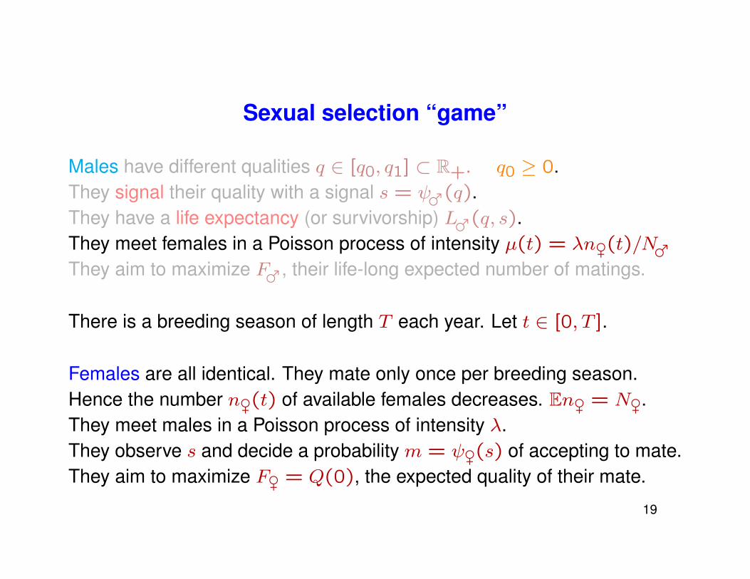
Sexual selection “game”

Males have different qualities q ∈ [q0, q1] ⊂ R+. q0 ≥ 0.They signal their quality with a signal s = ψ♂(q).They have a life expectancy (or survivorship) L♂(q, s).They meet females in a Poisson process of intensity µ(t) = λn♀(t)/N♂They aim to maximize F♂, their life-long expected number of matings.

There is a breeding season of length T each year. Let t ∈ [0, T ].

Females are all identical. They mate only once per breeding season.Hence the number n♀(t) of available females decreases. En♀ = N♀.They meet males in a Poisson process of intensity λ.They observe s and decide a probability m = ψ♀(s) of accepting to mate.They aim to maximize F♀ = Q(0), the expected quality of their mate.

17





18





19

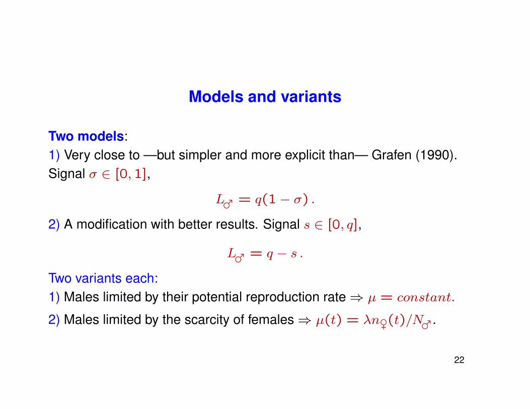
Models and variants

Two models:1) Very close to —but simpler and more explicit than— Grafen (1990).Signal σ ∈ [0,1],

L♂ = q(1− σ) .

2) A modification with better results. Signal s ∈ [0, q],

L♂ = q − s .

Two variants each:1) Males limited by their potential reproduction rate⇒ µ = constant.

2) Males limited by the scarcity of females⇒ µ(t) = λn♀(t)/N♂.

20

Models and variants


L♂ = q(1− σ) .


L♂ = q − s .



21

Models and variants


L♂ = q(1− σ) .


L♂ = q − s .



22

Females’ behaviour

Let Q(t) be the expected quality of her mate for a female that has not yetmated at time t ∈ [0, T ].

Q(t) = E[λdtmq + (1− λdtm)Q(t+ dt)] .

In the limit as dt→ 0, this yields

dQ

dt+ λE[m(q −Q(t))] = 0 , Q(T ) = 0 .

Females’ fitness Q(0) maximized by

m = ψ♀(q, t) =

{0 if q < Q(t) ,1 if q ≥ Q(t) ,

⇒ ψ?♀(s, t) =

{0 if s < χ(Q(t)) ,1 if s ≥ χ(Q(t)) .

Easy to integrate in closed form if P0 uniformly distributed over [q0, q1].23

Curves Q(t)Feuille1

Page 1

0 0,2 0,4 0,6 0,8 1 1,20

0,1

0,2

0,3

0,4

0,5

0,6

0,7

0,8

0,9

lambda T = 6lambda T = 8lambda T=10lambda T=12

Q(t)/q1 as a function of t/T for q0 = 0, for various values of λT .

24

Evolutionary dynamics ♀

Hypothesis The females’ behaviour is a behavioural trait, with an adapta-tion must faster than the males’ physical trait. (∼ Ecological vs genetic.)

⇒ the evolution of Females’ behaviour may be studied as if ψ♂ were fixed.

Because a female’s fitness does not depend on her conspecifics’ behaviour,adaptive dynamics are a gradient dynamics for F♀ = Q(0).

⇒ Easy to show convergence, for two scenarii (function-valued trait):Mixed strategy: ψ♀(s, t) = m ∈ [0,1].Threshold strategy: ψ♀(s, t) = Υ(s− θ(t)).Both evolve toward equilibrium threshold strategy.

25




Because a female’s fitness does not depend on her conspecifics’ behaviour,evolutionary dynamics are a gradient dynamics for F♀ = Q(0).


26




Because a female’s fitness does not depend on her conspecifics’ behaviour,evolutionary dynamics are a gradient dynamics for F♀ = Q(0).


27

Consequences for the males

A male of quality q only mates when t ≥ tm such that Q(tm) = q.Females leave the pool of available females at a rate

dN♀dt

=

−N♀λq1 −Q(t)

q1 − q0as long as Q(t) ≥ q0 ,

−λN♀ when Q(t) < q0 .

If scarcity of females is the limiting factor, Eµ(t) = λN♀(t)/N♂.

Males obtain a fitness F♂(q, s, ψ?♀(s, ·)) = L♂(q, s)Nm where

Nm =∫ Ttm

Eµ(t) dt .

In differentiating w.r.t s, remember that tm depends on χ which, at equilib-rium, must coincide with ψ?♂. Hence a differential equation for ψ?♂.

28



dN♀dt

=

−N♀λq1 −Q(t)





Nm =∫ Ttmµ(t) dt .


29



dN♀dt

=

−N♀λq1 −Q(t)





Nm =∫ Ttm

Eµ(t) dt .


30



dN♀dt

=

−N♀λq1 −Q(t)



If scarcity of females is the limiting factor, µ(t) = λN♀(t)/N♂.


Nm =∫ Ttm

Eµ(t) dt .


31

Miracle

Everything integrates in closed form forQ(t), N♀(t), and for ψ♂(q) all fourmodels × variants !

But more complicated for q0 > 0 than for q0 = 0, because all equationsare different when Q(t) < q0.

32

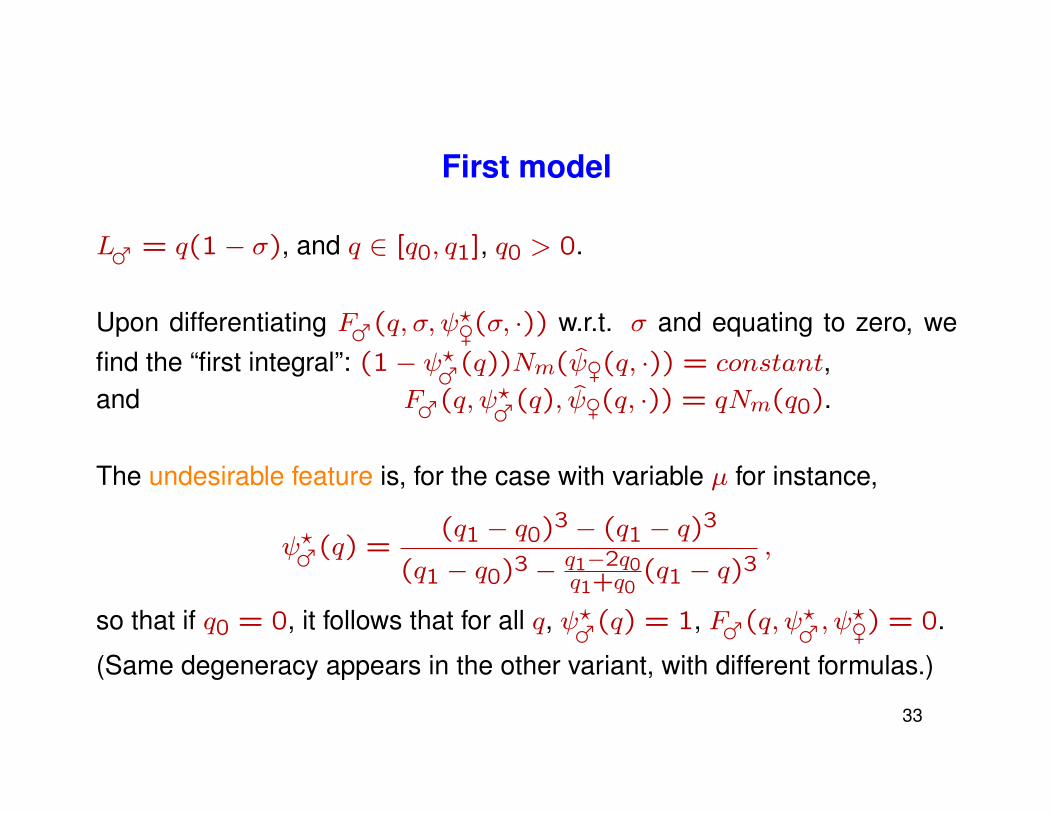
First model

L♂ = q(1− σ), and q ∈ [q0, q1], q0 > 0.

Upon differentiating F♂(q, σ, ψ?♀(σ, ·)) w.r.t. σ and equating to zero, wefind the “first integral”: (1− ψ?♂(q))Nm(ψ♀(q, ·)) = constant,and F♂(q, ψ?♂(q), ψ♀(q, ·)) = qNm(q0).

The undesirable feature is, for the case with variable µ for instance,

ψ?♂(q) =(q1 − q0)3 − (q1 − q)3

(q1 − q0)3 − q1−2q0q1+q0

(q1 − q)3,

so that if q0 = 0, it follows that for all q, ψ?♂(q) = 1, F♂(q, ψ?♂, ψ?♀) = 0.

(Same degeneracy appears in the other variant, with different formulas.)

33

Curves for the first model (variable µ)λT = 8Feuille4

Page 1

0 0,2 0,4 0,6 0,8 1 1,20

0,2

0,4

0,6

0,8

1

1,2

q0/q1 = 0,01q0/q1 = 0,1q0/q1 = 0,25q0/q1 = 0,5

ψ?♂ as a function of q/q1Feuille4

Page 1

0 0,2 0,4 0,6 0,8 1 1,20

0,1

0,2

0,3

0,4

0,5

0,6

q0/q1 = 0,01q0/q1 = 0,1q0/q1 = 0,25q0/q1 = 0,5

Feuille4

Page 1

0 0,2 0,4 0,6 0,8 1 1,20

0,01

0,02

0,03

0,04

0,05

0,06

0,07

0,08

q0/q1 = 0,01q0/q1 = 0,1q0/q1 = 0,25q0/q1 = 0,5

L♂ as a function of q/q1 F♂ as a function of q/q1.

34

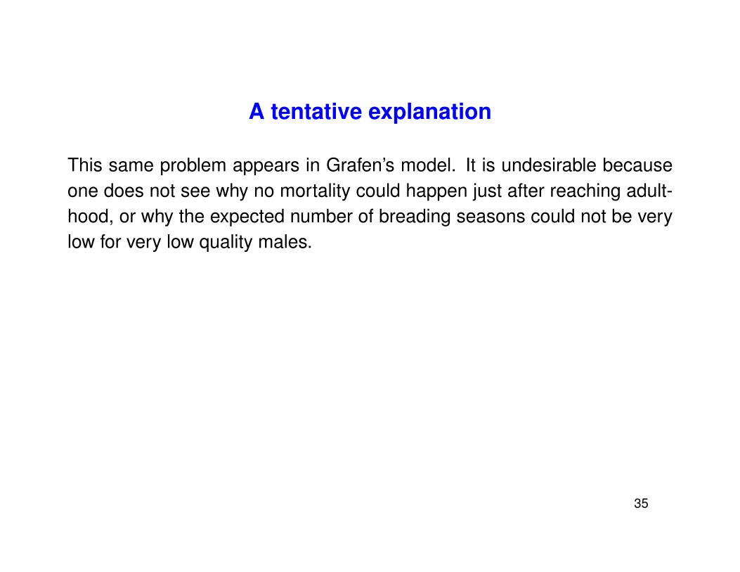
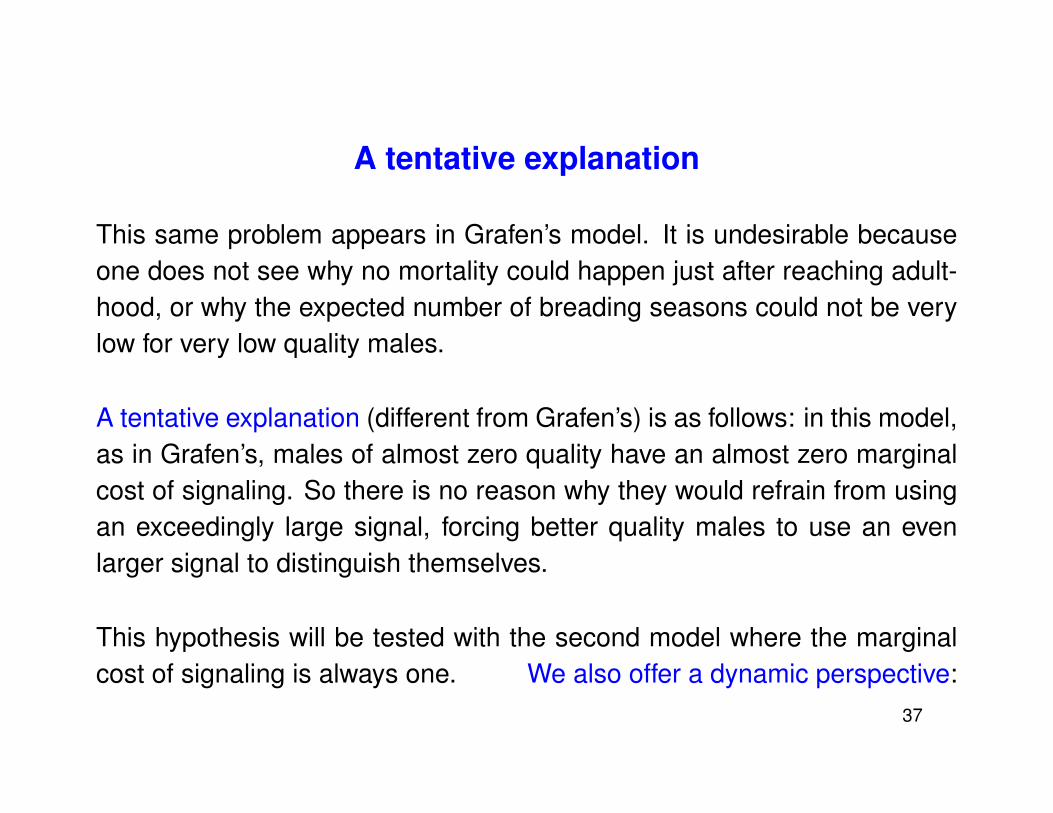
A tentative explanation

This same problem appears in Grafen’s model. It is undesirable becauseone does not see why no mortality could happen just after reaching adult-hood, or why the expected number of breading seasons could not be verylow for very low quality males.

A tentative explanation (different from Grafen’s) is as follows: in this model,as in Grafen’s, males of almost zero quality have an almost zero marginalcost of signaling. So there is no reason why they would refrain from usingan exceedingly large signal, forcing better quality males to use an evenlarger signal to distinguish themselves.

This hypothesis will be tested with the second model where the marginalcost of signaling is always one. We also offer a dynamic perspective:

35





36





37

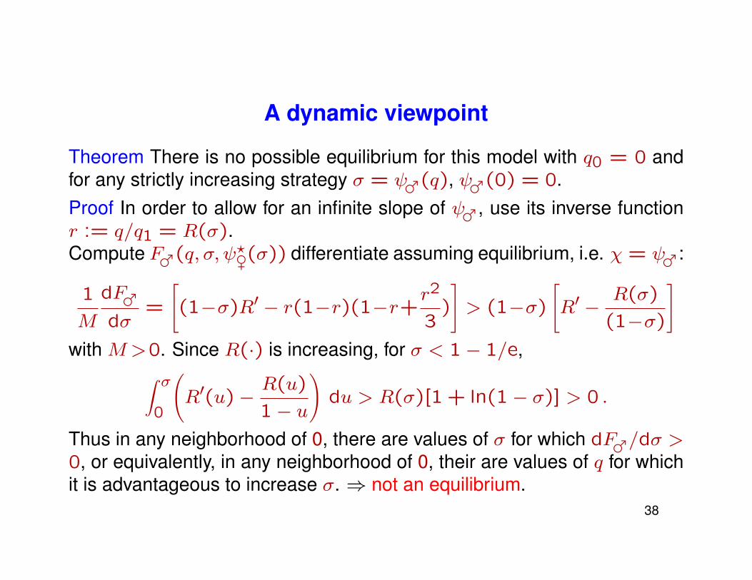
A dynamic viewpoint

Theorem There is no possible equilibrium for this model with q0 = 0 andfor any strictly increasing strategy σ = ψ♂(q), ψ♂(0) = 0.Proof In order to allow for an infinite slope of ψ♂, use its inverse functionr := q/q1 = R(σ).Compute F♂(q, σ, ψ?♀(σ)) differentiate assuming equilibrium, i.e. χ = ψ♂:

1

M

dF♂dσ

=

[(1−σ)R′ − r(1−r)(1−r+

r2

3)

]> (1−σ)

[R′ −

R(σ)

(1−σ)

]with M>0. Since R(·) is increasing, for σ < 1− 1/e,∫ σ

0

(R′(u)−

R(u)

1− u

)du > R(σ)[1 + ln(1− σ)] > 0 .

Thus in any neighborhood of 0, there are values of σ for which dF♂/dσ >0, or equivalently, in any neighborhood of 0, their are values of q for whichit is advantageous to increase σ. ⇒ not an equilibrium.

38

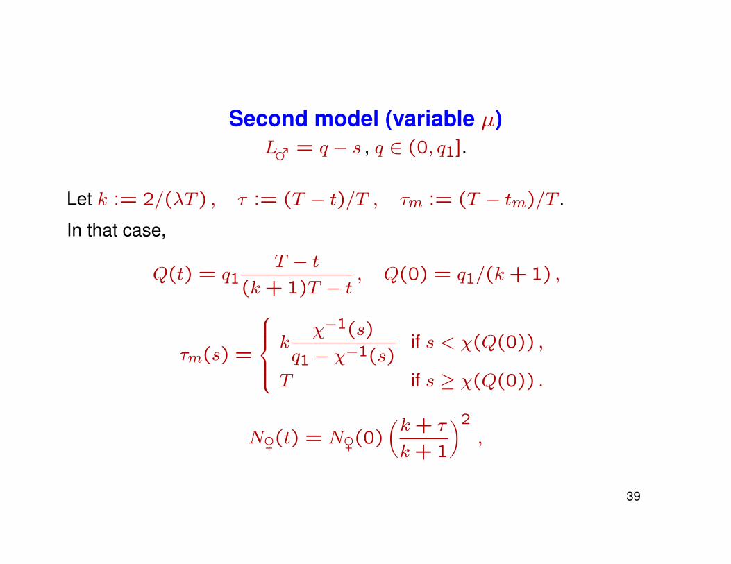
Second model (variable µ)L♂ = q − s , q ∈ (0, q1].

Let k := 2/(λT ) , τ := (T − t)/T , τm := (T − tm)/T .

In that case,

Q(t) = q1T − t

(k + 1)T − t, Q(0) = q1/(k + 1) ,

τm(s) =

k

χ−1(s)

q1 − χ−1(s)if s < χ(Q(0)) ,

T if s ≥ χ(Q(0)) .

N♀(t) = N♀(0)(k + τ

k + 1

)2,

39

Males’ strategy

F♂(q, s, ψ?♀(s)) =µ0T

(k + 1)2(q − s)(k2τm(s) + kτm(s)2 +

1

3τm(s)3) .

Differentiating F♂(q, s, ψ?♀(s)) and equating to zero, for s = ψ?♂(q),(and identifying χ(·) = ψ?♂(·)), we get,

ψ?♂′ = q3

1

q − ψ?♂(q)

q(q1 − q)(q21 − q1q + q2

3 ), ψ?♂(0) = 0 ,

for q ≤ Q(0) = q1/(k + 1), and ψ?♂(q) = constant for q ≥ Q(0).

Miracle This o.d.e. has a closed form solution, in terms of r := q/q1:

Ψ(q1r) = q127r + 18r2 + 9r3 + 3r4 − r6

2(27 + r6).

40

Males’ strategy

F♂(q, s, ψ?♀(s)) =µ0T

(k + 1)2(q − s)(k2τm(s) + kτm(s)2 +

1

3τm(s)3) .

Differentiating F♂(q, s, ψ?♀(s)) and equating to zero, for s = ψ?♂(q),(and identifying χ(·) = ψ?♂(·)), we get,

ψ?♂′ = q3

1

q − ψ?♂(q)

q(q1 − q)(q21 − q1q + q2

3 ), ψ?♂(0) = 0 ,

for q ≤ Q(0) = q1/(k + 1), and ψ?♂(q) = constant for q ≥ Q(0).

Miracle This o.d.e. has a closed form solution, in terms of r := q/q1:

Ψ(q1r) = q127r + 18r2 + 9r3 + 3r4 − r6

2(27 + r6).

41

Curves for the second model (both variants)λT = 8, Q(0) = .8

Feuille2

Page 1

0 0,2 0,4 0,6 0,8 1 1,20

0,1

0,2

0,3

0,4

0,5

0,6

0,7

0,8

fixed muvariable mu

ψ?♂/q1 as a function of q/q1Feuille2

Page 1

0 0,2 0,4 0,6 0,8 1 1,20

2

4

6

8

10

12

14

16

fixed muvariable mu

Feuille2

Page 1

0 0,2 0,4 0,6 0,8 1 1,20

20

40

60

80

100

120

fixed muvariable mu

L♂ as a function of q/q1 F♂ as a function of q/q1

42

Adaptive dynamics ♂


⇒ the evolution of Males’ behaviour may be studied as if χ(·) = ψ♂(·).

Hypothesis The genes responsible for males’ strategies are inherited fromthe father only,⇒ equivalent to “clonal” reproduction.

If mutation rate independent from q, adaptive dynamics yield a PDE(t = evolutionary time, r = q/q1):

∂ψ♂(r, t)

∂t=

M

(1− r)3

r − ψ♂ψ′♂(1− r)

− r + r2 −r3

3

.Work in progress . . .

43






∂ψ♂(r, t)

∂t=

M

(1− r)3

r − ψ♂(1− r)ψ′♂

− r + r2 −r3

3

.Asymptotic behaviour ? Work in progress . . .

44






∂ψ♂(r, t)

∂t=

M

(1− r)3

r − ψ♂(1− r)ψ′♂

− r + r2 −r3

3

.Asymptotic behaviour ? Work in progress . . .

45

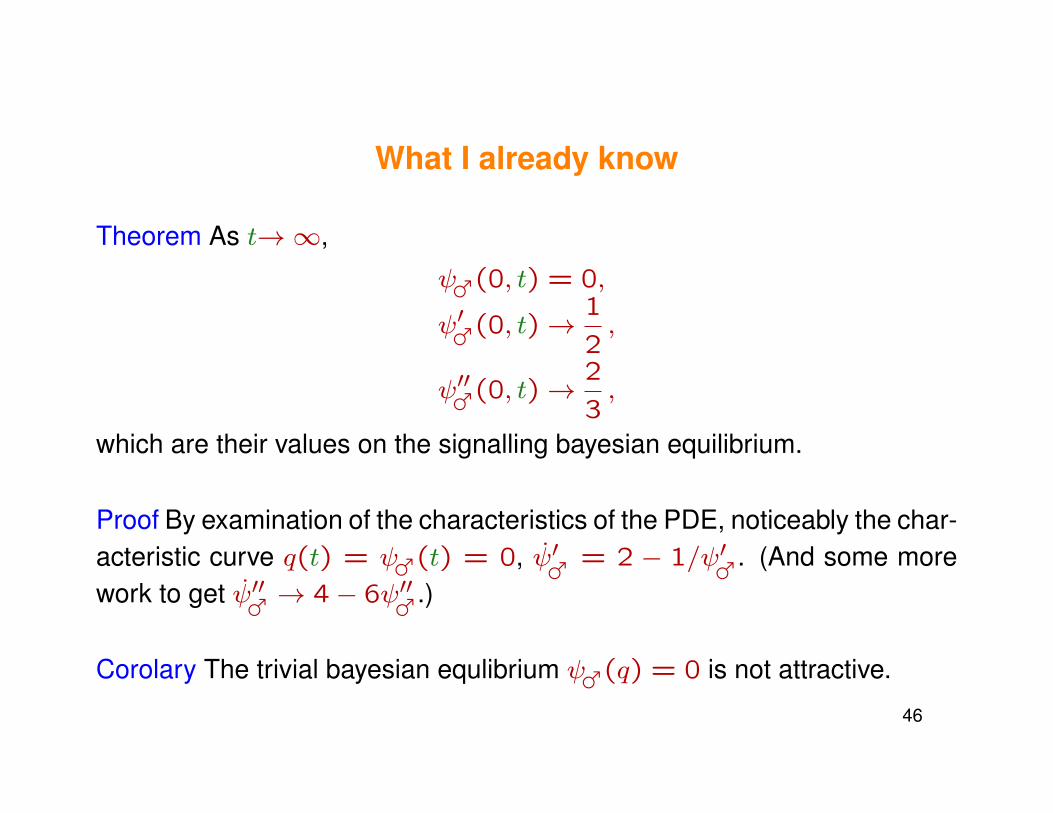
What I already know

Theorem As t→∞,

ψ♂(0, t) = 0,

ψ′♂(0, t)→1

2,

ψ′′♂(0, t)→2

3,

which are their values on the signalling bayesian equilibrium.

Proof By examination of the characteristics of the PDE, noticeably the char-acteristic curve q(t) = ψ♂(t) = 0, ψ′♂ = 2 − 1/ψ′♂. (And some morework to get ψ′′♂ → 4− 6ψ′′♂.)

Corolary The trivial bayesian equlibrium ψ♂(q) = 0 is not attractive.

46

What I proved after the workshop

Theorem Let 0 < p0 ≤ ψ′♂(q,0) < 1/2, then if ψ♂(·, t) for q ∈ [0, Q0]

converges as t→∞, it is towards Ψ(·).

Numerical evidence Numerical integration of the EDP of adaptive dynamics(via the method of characteristics) shows a very precise convergence ofψ♂ towards Ψ.

47

Documents

Games of sexual selection - Centre de Recherches · PDF file · 2013-11-20Games of sexual selection: static and dynamic aspects Pierre Bernhard & Fred´ eric Hamelin ... (1975):The