Embed Size (px)
Citation preview

GARCH models with dummiesA study of the impact of U.S. monetary policy on inflation
Scott [email protected]
April 26, 2006
Scott Deacle [email protected] () GARCH models with dummies April 26, 2006 1 / 47
Outline
1 ARCH and GARCH Models
2 Inflation Targeting and the October 1979 Reform of U.S. MonetaryPolicy
3 My Study
4 Conclusions
Scott Deacle [email protected] () GARCH models with dummies April 26, 2006 2 / 47
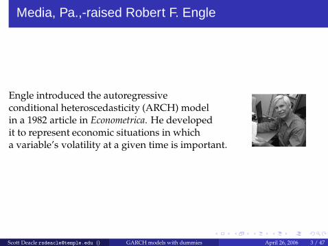
Media, Pa.,-raised Robert F. Engle
Engle introduced the autoregressiveconditional heteroscedasticity (ARCH) modelin a 1982 article in Econometrica. He developedit to represent economic situations in whicha variable’s volatility at a given time is important.
Scott Deacle [email protected] () GARCH models with dummies April 26, 2006 3 / 47

Friedman’s Hypothesis
When Engle introduced the ARCHmodel, macroeconomists were looking for ways tostudy inflation volatility. They were inspired in partby Milton Friedman’s Nobel Prize address (1977).Friedman proposed higher inflation causes greaterinflation volatility. The higher volatility then hasconsequences that reduce real output as economicagents devote resources to dealing with the risk of inflation, Friedmanargued.
In his 1982 article, Engle used an ARCHmodel to to study inflation in the United Kingdom.
Scott Deacle [email protected] () GARCH models with dummies April 26, 2006 4 / 47
Differences between ARCH and OLS
A simple regression model produces a constant unconditionalvariance of the independent variable. The ARCH model produces boththe unconditional variance and a process for the time-varyingconditional variance.
Scott Deacle [email protected] () GARCH models with dummies April 26, 2006 5 / 47
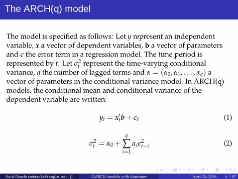
The ARCH(q) model
The model is specified as follows: Let y represent an independentvariable, x a vector of dependent variables, b a vector of parametersand ǫ the error term in a regression model. The time period isrepresented by t. Let σ2
t represent the time-varying conditionalvariance, q the number of lagged terms and α = (α0, α1, . . . , αq) avector of parameters in the conditional variance model. In ARCH(q)models, the conditional mean and conditional variance of thedependent variable are written:
yt = x′tb + ǫt (1)
σ2t = α0 +
q
∑i=1
αiǫ2t−i (2)
Scott Deacle [email protected] () GARCH models with dummies April 26, 2006 6 / 47
The Conditional Variance Term
The conditional variance is not heteroscedastic with respect to x. Itis heteroscedastic with respect to its q lagged values.
The conditional variance grows and shrinks according to themagnitude of past shocks. This makes the model realistic forvariables for which large shocks occur in clusters. It givesresearchers a measure of the volatility of the dependent variableat each observation.
Scott Deacle [email protected] () GARCH models with dummies April 26, 2006 7 / 47

Stationarity and unconditional variance
The error process is assumed to be weakly stationary.
E[ǫt] = 0 (3)
Var[ǫt] = σ2t (4)
Cov[ǫt, ǫs] = 0, t 6= s (5)
It can also be shown that the unconditional variance is
Var[ǫt] = σ2t =
α0
1 − ∑qi=1 αi
(6)
Scott Deacle [email protected] () GARCH models with dummies April 26, 2006 8 / 47

Detecting ARCH
The presence of an ARCH process may be detected through visual andanalytic means. For starters, one may inspect a time series plot of thedependent variable for clusters of large movements.
Scott Deacle [email protected] () GARCH models with dummies April 26, 2006 9 / 47

Log Difference of GDP DeflatorVertical line marks start ofVolcker reform
U.S. Inflation, 1948:2-2005:4
1948 1953 1958 1963 1968 1973 1978 1983 1988 1993 1998 2003-5.0
-2.5
0.0
2.5
5.0
7.5
10.0
12.5
15.0
Scott Deacle [email protected] () GARCH models with dummies April 26, 2006 10 / 47
Detecting ARCH
One may also plot the squared residuals from the ordinary leastsquares estimate of the conditional mean model. Clusters of largevalues indicate the presence of ARCH.
Scott Deacle [email protected] () GARCH models with dummies April 26, 2006 11 / 47
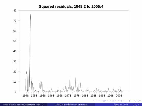
Squared residuals, 1948:2 to 2005:4
1948 1953 1958 1963 1968 1973 1978 1983 1988 1993 1998 20030
10
20
30
40
50
60
70
80
Scott Deacle [email protected] () GARCH models with dummies April 26, 2006 12 / 47
Analytic test for ARCH
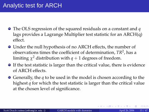
The OLS regression of the squared residuals on a constant and qlags provides a Lagrange Multiplier test statistic for an ARCH(q)effect.
Under the null hypothesis of no ARCH effects, the number ofobservations times the coefficient of determination, TR2, has alimiting χ2 distribution with q + 1 degrees of freedom.
If the test statistic is larger than the critical value, there is evidenceof ARCH effects.
Generally, the q to be used in the model is chosen according to thehighest q for which the test statistic is larger than the critical valueat the chosen level of significance.
Scott Deacle [email protected] () GARCH models with dummies April 26, 2006 13 / 47

What was wrong with ARCH
ARCH models often require relatively long lags in the conditionalvariance equations. In early work with ARCH models, researchersoften imposed arbitrarily weighted and fixed lag structures on theconditional variance equation to avoid negative unconditionalvariance estimates (see, for example, Engle and Kraft (1983)).
Four years after the introduction of ARCH,Engle’s graduate student Tim Bollerslev addressedthis issue with the generalized autoregressiveconditional heteroscedasticity (GARCH) model.
Scott Deacle [email protected] () GARCH models with dummies April 26, 2006 14 / 47

The GARCH(p,q) model
In GARCH(p,q) models, the conditional variance equation is extendedto include p lagged values of the conditional variance.
yt = x′tb + ǫt (7)
σ2t = α0 +
q
∑i=1
αiǫ2t−i +
p
∑j=1
βjσ2t−j (8)
Scott Deacle [email protected] () GARCH models with dummies April 26, 2006 15 / 47
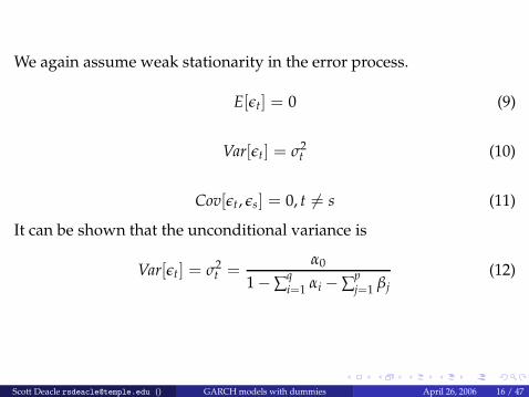
We again assume weak stationarity in the error process.
E[ǫt] = 0 (9)
Var[ǫt] = σ2t (10)
Cov[ǫt, ǫs] = 0, t 6= s (11)
It can be shown that the unconditional variance is
Var[ǫt] = σ2t =
α0
1 − ∑qi=1 αi − ∑
pj=1 βj
(12)
Scott Deacle [email protected] () GARCH models with dummies April 26, 2006 16 / 47
The Advantage of GARCH(p,q) models
This allows the entire history of past shocks to influence the currentvalue of the conditional variance. Bollerslev showed a GARCH modelwith a small number of terms may be more efficient than an ARCHmodel with many terms.
Scott Deacle [email protected] () GARCH models with dummies April 26, 2006 17 / 47
ARCH and GARCH estimation
Maximum likelihood estimators of ARCH(q) and GARCH(p,q)models are more efficient than ordinary least squares. BecauseOLS estimates are consistent, they may be used as starting valuesfor maximum likelihood estimation.
Maximum likelihood estimation of ARCH(q) models may beperformed by maximization of the log likelihood function orusing a four-step procedure based on the method of scoringshown in Engle (1982). See also Dr. Buck’s notes.
Scott Deacle [email protected] () GARCH models with dummies April 26, 2006 18 / 47

ARCH and GARCH estimation
Maximum likelihood estimation of GARCH models iscomplicated by the presence of lagged values of the conditionalvariance term in the conditional variance equation. (Try setting itup sometime in MathCAD, and you’ll see what I mean).Numerical methods (discussed later) are usually employed to findthe parameter estimates.
I was most successful in using RATS to estimate my GARCHmodels. Estima (the company that writes RATS) has some usefulsample programs on its Web site.
Scott Deacle [email protected] () GARCH models with dummies April 26, 2006 19 / 47

Detecting GARCH
The same methods discussed above for detecting ARCH may be usedto look for evidence of GARCH effects. If the Lagrange Multiplier teststatistic gives evidence of ARCH for q of four or more, a GARCHmodel is probably more appropriate.
Scott Deacle [email protected] () GARCH models with dummies April 26, 2006 20 / 47

Verifying ARCH and GARCH
The Ljung-Box Q-statistic may be used to verify the appropriateness ofthe model’s specification. After estimation of an an ARCH or GARCHmodel, the Ljung-Box Q-statistic is calculated by regressing theresiduals on a constant and their lagged values. If the Q-statistic isgreater than its χ2 critical value, one should reject the null hypothesisof no autocorrelation in the residuals. This suggests the GARCHmodel is misspecified since the residuals are not weakly stationarity.
Scott Deacle [email protected] () GARCH models with dummies April 26, 2006 21 / 47
ARCH and GARCH’s popularity
Variations on the basic ARCH and GARCH models have beendeveloped to better study particular theories and types of data. ARCHand GARCH models have been especially useful for assessing the riskof an investment portfolio. As a portfolio’s returns become morevolatile, the conditional variance term produced by GARCH modelsprovides wider forecast confidence intervals. This contrasts with therelatively stable ordinary least squares forecast ranges that give lessinformation about portfolio risk.
The ability of GARCH models to account for volatility clustering alsomakes it useful for studying inflation and uncertainty. The next threeslides show forecast confidence intervals for U.S. inflation. The OLSforecast intervals stay constant throughout the time series. TheGARCH forecast intervals widen in times of high volatility andnarrow in times of low volatility. This may be a good way to modeluncertainty about future inflation.
Scott Deacle [email protected] () GARCH models with dummies April 26, 2006 22 / 47

Inflation Upper Bound Lower Bound
Actual inflation and OLS confidence intervals
1948 1953 1958 1963 1968 1973 1978 1983 1988 1993 1998 2003-15
-10
-5
0
5
10
15
20
25
Actual Inflation Upper Bound Lower Bound
Actual Inflation and GARCH(1,1) Confidence Intervals
1948 1953 1958 1963 1968 1973 1978 1983 1988 1993 1998 2003-15
-10
-5
0
5
10
15
20
25
Scott Deacle [email protected] () GARCH models with dummies April 26, 2006 23 / 47

Inflation Upper Bound Lower Bound
Actual inflation and OLS confidence intervals
1948 1953 1958 1963 1968 1973 1978 1983 1988 1993 1998 2003-15
-10
-5
0
5
10
15
20
25
Scott Deacle [email protected] () GARCH models with dummies April 26, 2006 24 / 47
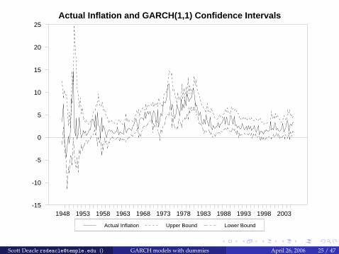
Actual Inflation Upper Bound Lower Bound
Actual Inflation and GARCH(1,1) Confidence Intervals
1948 1953 1958 1963 1968 1973 1978 1983 1988 1993 1998 2003-15
-10
-5
0
5
10
15
20
25
Scott Deacle [email protected] () GARCH models with dummies April 26, 2006 25 / 47

Recommended reading
Greene (2003), Econometric Analysis, Fifth Edition, pp. 238-246.
Engle (1982), Autoregressive conditional heteroscedasticity withestimates of the variance of United Kingdom inflation,Econometrica, 50, 987-1008.
Dr. Buck’s lecture notes.
Engle (2001), GARCH 101: The use of ARCH/GARCH Models inapplied econometrics, Journal of Economic Perspectives
Bollerslev (1986), Generalized autoregressive conditionalheteroscedasticity, Journal of Econometrics, 31, 307-327. Not freely
available online through Temple.
Scott Deacle [email protected] () GARCH models with dummies April 26, 2006 26 / 47

The October 1979 Reform of U.S. Monetary Policyand
Inflation Targeting
Scott Deacle [email protected] () GARCH models with dummies April 26, 2006 27 / 47
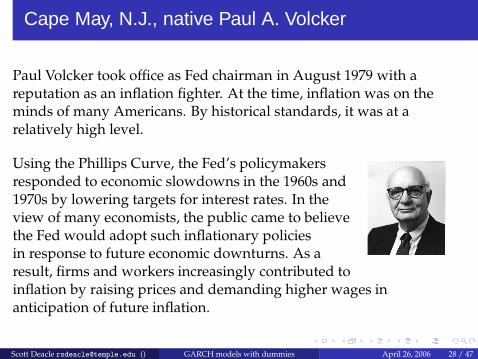
Cape May, N.J., native Paul A. Volcker
Paul Volcker took office as Fed chairman in August 1979 with areputation as an inflation fighter. At the time, inflation was on theminds of many Americans. By historical standards, it was at arelatively high level.
Using the Phillips Curve, the Fed’s policymakersresponded to economic slowdowns in the 1960s and1970s by lowering targets for interest rates. In theview of many economists, the public came to believethe Fed would adopt such inflationary policiesin response to future economic downturns. As aresult, firms and workers increasingly contributed toinflation by raising prices and demanding higher wages inanticipation of future inflation.
Scott Deacle [email protected] () GARCH models with dummies April 26, 2006 28 / 47
Changes in monetary policy
Volcker called emergency meetings of the open market committee andBoard of Governors on October 9, 1979. The governors votedunanimously to raise target interest rates one percent. They alsochanged their tactics for influencing the money supply. Publicstatements following the meeting emphasized the Fed’s determinationto lower the inflation rate.
In the years following the October 1979 policy change, estimates ofU.S. inflation dropped from a range between 5 and 12 percent to arange between 1 and 4 percent, where they have stayed for the last 15years.
Scott Deacle [email protected] () GARCH models with dummies April 26, 2006 29 / 47

Inflation targeting
Many other countries have tried a different tactic to control inflation.Led by New Zealand in 1990, these countries’ central banks adoptedpublicly announced inflation rate targets.
The fundamental argument in support of inflationtargeting is that targets will cause the publicto believe the government will try to keep inflationlow. The public will then raise prices and wagesat relatively low rates, contributing to overall pricestability. Some proponents of inflation targetingsay the practice improves economic performance byreducing uncertainty about inflation.
Current Fed chairman Ben S. Bernanke (who used tolive in Princeton, N.J.,) supports inflation targeting.
Scott Deacle [email protected] () GARCH models with dummies April 26, 2006 30 / 47
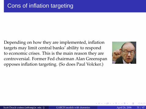
Cons of inflation targeting
Depending on how they are implemented, inflationtargets may limit central banks’ ability to respondto economic crises. This is the main reason they arecontroversial. Former Fed chairman Alan Greenspanopposes inflation targeting. (So does Paul Volcker.)
Scott Deacle [email protected] () GARCH models with dummies April 26, 2006 31 / 47
Do we need inflation targeting when we have PaulVolcker?
Kontonikas (2004) uses several variations on the basic GARCH modelto study the impact of inflation targeting on inflation and inflationuncertainty in the United Kingdom. He concludes that after theannouncement of inflation targeting, U.K. inflation becamesubstantially less persistent and less variable. He also finds asignificant negative impact from inflation targeting on long-rununcertainty as measured by the GARCH conditional variance.
One of the goals of this paper is to use similar methods to study theeffect on the U.S. of the 1979 reforms and the ensuing years ofanti-inflationary policy. Did Volcker’s reforms and Greenspan’spolicies have an effect similar to that Kontonikas found from inflationtargeting? And is there a negative relationship in the U.S. betweeninflation variance and the level of inflation?
Scott Deacle [email protected] () GARCH models with dummies April 26, 2006 32 / 47

Data
An implicit GDP deflator was calculated from quarterly Bureau ofEconomic Analysis data (1947:1 to 2005:4, 236 observations) on realand nominal GDP.
Deflator =NominalGDP
RealGDP∗ 100 (13)
Quarterly inflation rates (235 observations) were calculated by takingthe log differences of successive quarterly deflators.
A dummy variable was also created, taking the value zero from 1947:1to 1979:4 and one from 1980:1 to 2005:4. The variable’s valuescorrespond to the periods before and after the October 1979 reform.
Scott Deacle [email protected] () GARCH models with dummies April 26, 2006 33 / 47
My GARCH(1,1)-M model, with a dummy variable
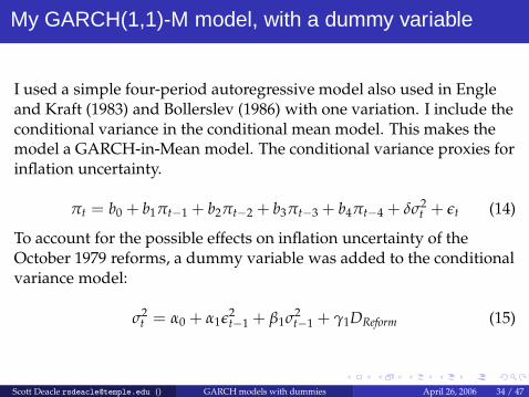
I used a simple four-period autoregressive model also used in Engleand Kraft (1983) and Bollerslev (1986) with one variation. I include theconditional variance in the conditional mean model. This makes themodel a GARCH-in-Mean model. The conditional variance proxies forinflation uncertainty.
πt = b0 + b1πt−1 + b2πt−2 + b3πt−3 + b4πt−4 + δσ2t + ǫt (14)
To account for the possible effects on inflation uncertainty of theOctober 1979 reforms, a dummy variable was added to the conditionalvariance model:
σ2t = α0 + α1ǫ2
t−1 + β1σ2t−1 + γ1DReform (15)
Scott Deacle [email protected] () GARCH models with dummies April 26, 2006 34 / 47
Lagrange Multiplier test
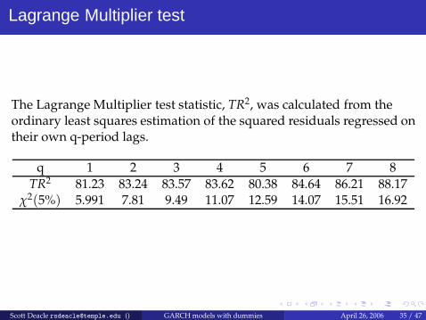
The Lagrange Multiplier test statistic, TR2, was calculated from theordinary least squares estimation of the squared residuals regressed ontheir own q-period lags.
q 1 2 3 4 5 6 7 8
TR2 81.23 83.24 83.57 83.62 80.38 84.64 86.21 88.17χ2(5%) 5.991 7.81 9.49 11.07 12.59 14.07 15.51 16.92
Scott Deacle [email protected] () GARCH models with dummies April 26, 2006 35 / 47
Maximum likelihood estimation
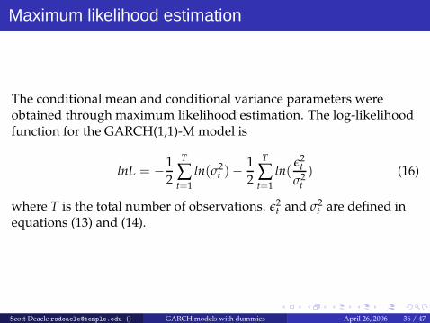
The conditional mean and conditional variance parameters wereobtained through maximum likelihood estimation. The log-likelihoodfunction for the GARCH(1,1)-M model is
lnL = −1
2
T
∑t=1
ln(σ2t )−
1
2
T
∑t=1
ln(ǫ2
t
σ2t
) (16)
where T is the total number of observations. ǫ2t and σ2
t are defined inequations (13) and (14).
Scott Deacle [email protected] () GARCH models with dummies April 26, 2006 36 / 47

The BHHH algorithm
The presence of a recursive term in the conditional variance equationcomplicates the optimization of the log likelihood function. FollowingBollerslev (1986), the optimization was performed with the Berndt,Hall, Hall and Hausman (BHHH) iterative algorithm. Let l denote thelikelihood function and θ(i) denote the parameter estimates after the ithiteration. The BHHH algorithm calculates the estimators according to
θ(i+1) = θ(i) + λi(T
∑i=1
∂lt∂θ
∂lt∂θ′
)−1T
∑i=1
∂lt∂θ
(17)
where ∂lt∂θ is evaluated at θ(i) and λi is a variable step length chosen to
maximize the likelihood function in the given direction.
Scott Deacle [email protected] () GARCH models with dummies April 26, 2006 37 / 47

Results
The effect of conditional variance, or uncertainty, represented by δ, onthe level of inflation is negative but not significant.
Table: Conditional Mean Parameter Estimates
b0 b1 b2 b3 b4 δ
0.518∗ 0.468∗∗ 0.183∗ 0.277∗∗ −0.001 −0.065(1.98) (6.89) (2.34) (4.37) (−1.03) (−0.93)
LL = −165.92 , Q(1) = 5.688∗∗, Q(6) = 9.247∗∗, Q(12) = 30.552*, ** denotes significant at 5% level, 1% level
Scott Deacle [email protected] () GARCH models with dummies April 26, 2006 38 / 47

Results
The effect of the reform dummy variable, represented by γ1, isnegative but not significant. The Q statistics indicate the modeleliminates autocorrelation of residuals up to six periods in the past.
Table: Conditional Variance Parameter Estimates
α0 α1 β1 γ1
0.564∗∗ 0.467∗∗ 0.350∗ −0.318(2.60) (2.96) (2.28) (−1.79)
*, ** denotes significant at 5% level, 1% level
Scott Deacle [email protected] () GARCH models with dummies April 26, 2006 39 / 47

Results
The federal government imposed price controls during the KoreanWar. The price controls likely brought a sharp reduction in inflationthat may have been expected. The government also imposed pricecontrols during parts of the 1960s and early 1970s. The price controlsmay cause the model to overstate the conditional variance of inflationduring those times. This in turn may cause the reduction in inflationvolatility from the Volcker reforms to be understated.
Scott Deacle [email protected] () GARCH models with dummies April 26, 2006 40 / 47

An alternative model
To correct for this in an early ARCH study of U.S. inflation, Engle(1983) added dummy variables to the conditional variance modelduring the approximate periods of price controls: 1951:2 to 1953:2,1962:1 to 1968:4 and 1971:2 to 1973:2. Dummy variables were added tothe GARCH(1,1)-M model’s conditional variance equations for thesame time periods to give
σ2t = α0 + α1ǫ2
t−1 + β1σ2t−1 + γ1DReform + γ2DPC1 + γ3DPC2 + γ4DPC3
(18)where DPC1, DPC2 and DPC3 represent respectively the dummyvariables for the first, second and third price control eras.
Scott Deacle [email protected] () GARCH models with dummies April 26, 2006 41 / 47
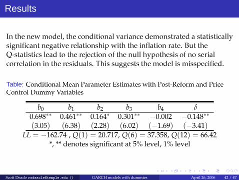
Results
In the new model, the conditional variance demonstrated a statisticallysignificant negative relationship with the inflation rate. But theQ-statistics lead to the rejection of the null hypothesis of no serialcorrelation in the residuals. This suggests the model is misspecified.
Table: Conditional Mean Parameter Estimates with Post-Reform and PriceControl Dummy Variables
b0 b1 b2 b3 b4 δ
0.698∗∗ 0.461∗∗ 0.164∗ 0.301∗∗ −0.002 −0.148∗∗
(3.05) (6.38) (2.28) (6.02) (−1.69) (−3.41)LL = −162.74 , Q(1) = 20.717, Q(6) = 37.358, Q(12) = 66.42
*, ** denotes significant at 5% level, 1% level
Scott Deacle [email protected] () GARCH models with dummies April 26, 2006 42 / 47
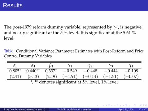
Results
The post-1979 reform dummy variable, represented by γ1, is negativeand nearly significant at the 5 % level. It is significant at the 5.61 %level.
Table: Conditional Variance Parameter Estimates with Post-Reform and PriceControl Dummy Variables
α0 α1 β1 γ1 γ2 γ3 γ4
0.805∗ 0.440∗∗ 0.337∗ −0.549 −0.448 −0.444 −0.108(2.41) (3.13) (2.19) (−1.91) (−0.14) (−1.51) (−0.07)
*, ** denotes significant at 5% level, 1% level
Scott Deacle [email protected] () GARCH models with dummies April 26, 2006 43 / 47
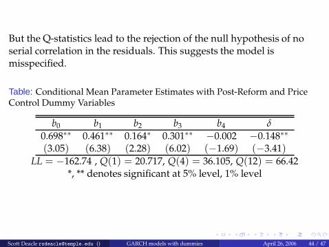
But the Q-statistics lead to the rejection of the null hypothesis of noserial correlation in the residuals. This suggests the model ismisspecified.
Table: Conditional Mean Parameter Estimates with Post-Reform and PriceControl Dummy Variables
b0 b1 b2 b3 b4 δ
0.698∗∗ 0.461∗∗ 0.164∗ 0.301∗∗ −0.002 −0.148∗∗
(3.05) (6.38) (2.28) (6.02) (−1.69) (−3.41)LL = −162.74 , Q(1) = 20.717, Q(4) = 36.105, Q(12) = 66.42
*, ** denotes significant at 5% level, 1% level
Scott Deacle [email protected] () GARCH models with dummies April 26, 2006 44 / 47
Conclusions
The first GARCH(1,1)-M model did not produce evidence thatlower inflation volatility is related to a lower inflation rate. Nordid it produce evidence that inflation was significantly lessvolatile after the reforms.
After controlling for possible distortions from price controls, theresults changed. Inflation volatility was found to have asignificant negative effect on inflation. The era after the 1979reform was found to have lower inflation volatility at a nearlyconventional level of statistical significance. The Ljung-Boxstatistic, however, suggests the second model is misspecified.
Scott Deacle [email protected] () GARCH models with dummies April 26, 2006 45 / 47
Results
Combined with Kontonikas’s results, this study suggests inflationtargeting is more effective at lowering inflation and inflationuncertainty than a firmly anti-inflation discretionary policy.
The lack of signifcant results could be due to model specification.Kontonikas relied heavily on Akaike-Schwarz information criteriato determine the lags he used in his autoregressive models. Healso used the component GARCH-M model of Engle and Lee(1993) to separate inflation volatility into short-term andlong-term components. He finds inflation targeting had a moresignificant negative effect on long-term uncertainty thanshort-term.
Scott Deacle [email protected] () GARCH models with dummies April 26, 2006 46 / 47

Results
This study could by extended by performing estimates usingmonthly data as well as other measures of prices such as theconsumer and producer price indices.
Alternative specifications of the conditional mean may provide abetter model. Including variables such as wages, import pricesand oil prices could affect the results.
It is also worth examining the possibility that the model of U.S.inflation should change over time.
Scott Deacle [email protected] () GARCH models with dummies April 26, 2006 47 / 47
A few closing thoughts
It is also worth noting how American public attitude toward inflationhas changed since the 1970s. A recent newspaper column (Samuelson2004) quotes polling expert Daniel Yankelovich, who wrote in 1979,"For the public today, inflation has the kind of dominance that no otherissue has had since World War II. . . . It would be necessary to go backto the 1930’s and the Great Depression to find a peacetime issue thathas had the country so concerned and distraught."
Today, inflation is rarely mentioned as a serious complicating factor inbusiness transactions or as an issue that needs the attention of thegovernment. This suggests, regardless of the findings of theseeconometric models, the public has more certain expectations aboutinflation now than when Paul Volcker took office. On the other hand,these results could show that the American public was too concernedabout inflation in the late 1970s.
Scott Deacle [email protected] () GARCH models with dummies April 26, 2006 48 / 47