Investigation of convective transport in the so-called

“gas diffusion layer” used in polymer electrolyte fuel cell

Otavio Beruski,1, ∗ Thiago Lopes,1, 2, † Anthony R. J. Kucernak,2, ‡ and Joelma Perez1, §

1Instituto de Quımica de Sao Carlos, Universidade de Sao Paulo,

13566-590, Sao Carlos, Sao Paulo, Brazil

2Department of Chemistry, Imperial College London,

South Kensington Campus, London SW7 2AZ, UK

Abstract

Recent experimental data on a fuel cell-like system revealed insights on the fluid flow in both free

and porous media. A computational model is used to investigate the momentum and species trans-

port in such system, solved using the finite elements method. The model consists of a stationary,

isothermal, diluted species transport in free and porous media flow. The momentum transport is

treated using different formulations, namely Stokes-Darcy, Darcy-Brinkman, and a hybrid Stokes-

Brinkman formulations. The species transport is given by the advection equation for a reactant

diluted in air. The formulations are compared to each other and to the available experimental data,

where it is concluded that the Darcy-Brinkman formulation reproduces the data appropriately. The

validated model is used to investigate the contribution of convection in reactant transport in porous

media of fuel cells. Convective transport provides a major contribution to reactant distribution in

the so-called diffusion media. For a serpentine channel and flow with Re = 260 to 590, convection

accounts for 29 to 58% of total reactant transport to the catalyst layer.

∗ oberuski@usp.br† tlopeschem@gmail.com; Presently at: Nuclear and Energy Research Institute, IPEN/CNEN-SP, 05508-

000, Sao Paulo, Sao Paulo, Brazil‡ anthony@imperial.ac.uk§ jperez@iqsc.usp.br

1

I. INTRODUCTION

Despite the great promise and effort involving the commercialization and deployment

of fuel cell technologies, several issues remains to be understood before one can say that

control over these systems has been achieved [1]. Different approaches are being explored,

and one such approach involves the use of computer models to assist in the interpretation

of experimental data, and possibly predict optimum design and conditions. Indeed, great

effort has been seen in the development of ab initio and semi-empirical models for fuel cell

systems, as exemplified by the compiled data and references in [2–5], and, more recently, in

[1]. These evidently points out the amount of work still needed to be done in theoretical,

computational and experimental approaches, but also highlights the benefits of coupling

these, and the need to do so.

As pointed out by Weber et al.[1], modelling is heavily dependent on experimental results,

from the input parameters to insights related to the mathematical description of physical

phenomena that may occur in the experimental device. Therefore, validation is extremely

important, in order to assure that the model complies with the physical effects observed in

reality, both locally and globally. That being said, the desired, in situ data is remarkably

difficult to obtain reliably. The impressive degree of variability in design, operational con-

ditions and experimental systems turns the validation into a problem by itself, given that,

usually, only part of the measurements and properties are experimentally available for spe-

cific devices. In fact, for complex, multiphysics systems, such as fuel cells, one would hope

to validate each aspect of the mathematical approach used, independently; however results

to allow for such independent assessments are rare.

Recently a promising experimental setup to allow probing and in situ observation of

fluid flow in fuel cell-like systems was published by some of us[6]. This approach used an

allotrope of oxygen to mimic the flow of oxygen through a fuel cell replica. In this case,

ozone (O3) diluted in air, was used as tracer, and a coumarin-based dye as the sensor to map

the local concentration of O3. The O3 interacts with the dye in a porous layer, similarly to

dioxygen and a metal- or carbon-based catalyst layer in a fuel cell, resulting in the emission

of photons, and the degradation of both reactant and catalyst. Measuring the light emission

from this “catalyst layer” allowed determination of the local O3 concentration and thus,

the flow dynamics in a system very similar to a fuel cell cathode operating in a regime in

2

which flooding does not occur. It was proposed that, contrary to what is usually assumed,

convection plays a significant role in the distribution of reactants in the porous layers. The

unique data reported in [6] is welcome amidst a gap in research of such aspects in the field,

providing an opportunity to further refine computational models for fuel cell-like systems,

enabling the validation of momentum and species transport in both global and local aspects.

As reported in the review by Weber and Newman in 2004[2], the majority of fuel cell

models treat species transport in the porous domains solely by diffusion, with some models

coupling it to Darcy’s law. In 2014, Weber et al.[1] stated that the usual approach for

momentum transport modelling is through Navier-Stokes equations coupled to Darcy’s law,

sometimes called Stokes-Darcy (SD) formulation. Indeed, it is seen that SD is widely used in

fuel cell models, e.g. Rawool and co-workers[7] and more recently described in [8], and also for

related systems, for instance the work of Knehr and collaborators in vanadium flow cells[9].

On the other hand, there are systems that do not necessarily make use of porous media. The

work of Braff and colleagues[10] is such an example, studying membraneless flow cells. The

authors study convection through boundary layer analysis, deriving analytical equations for

fast examination of experimental systems. The correct description of momentum transport

is, particularly in this case, essential to properly account for species transport.

It is underappreciated, though, that in order to couple the velocity fields near the interface

between the free and porous domains, it is necessary to introduce appropriate boundary con-

ditions. Two such interfacial models are compared by Le Bars and Worster[11], namely one

from Beavers and Joseph[12] and another proposed by the authors, where the latter is shown

to be more accurate. An alternative to the SD formulation is the so-called Darcy-Brinkman

(DB) formulation[11], where both free and porous media flow are treated simultaneously,

therefore eliminating the need for an explicit boundary condition for the velocity field near

the interface. It can also be shown that the DB formulation reverts to the SD as the per-

meability approaches zero, or as particle size becomes very large, making it a more general

approach[11]. In fact, the boundary conditions discussed in [11] are compared to the DB

formulation, in order to assess its accuracy. In light of this, one would expect the DB as

preferable for momentum transport modelling in fuel cells, however it seems that no thor-

ough validation of its use in these systems has been made, and few works have been found

to actually use it[13, 14]. On the other hand, the wide range of length scales known to exist

in fuel cells favours the multiple-domain SD approach, allowing for a better description of

3

the flow variables in each domain. In this case, the correct choice of interfacial boundary

conditions should be important for fuel cell modelling.

In order to explore the differences between the outlined approaches, a macroscopic, finite

elements-based model was assembled to simulate the species and flow dynamics of the system

reported in [6]. Using the available data to validate the approach, the intent is to assist in

the understanding of the system, and, ultimately, jointly provide a consistent tool to study

the dynamics of fuel cell-like systems. The remainder of this work is organized as follows.

The mathematical formulations used in the model are presented in Section II, along with

remarks regarding the geometry and parameters used in the simulations. In Section III,

the model is compared to the available experimental data, in order to choose a suitable,

validated formulation. The validated model is then used to assess the hypothesis raised in

the experimental work, providing a discussion regarding the existence, or not, of postulated

phenomena in the reported system and its implications in an actual fuel cell. Section IV

presents the final remarks and perspectives to this work.

II. METHODS

All finite element calculations were performed using the commercial software COMSOL

Multiphysicsr 5.1, along with the CFD, and Batteries and Fuel Cell modules. Unless oth-

erwise noted, default parameters are assumed. The mathematical framework used has been

recently revised by Weber et al.[1] for fuel cell systems, and a detailed description may

be found in it and references therein, while Le Bars and Worster[11] provides a derivation

and discussion regarding the Darcy-Brinkman formulation and the interface boundary con-

ditions. Details regarding the implementation may be found on the software’s reference

manual[15] and the modules user’s guides[16, 17]. The remainder data manipulation was

performed using the R2012a version of MATLABr.

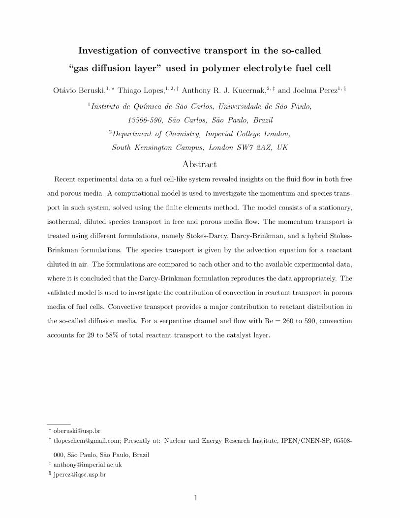
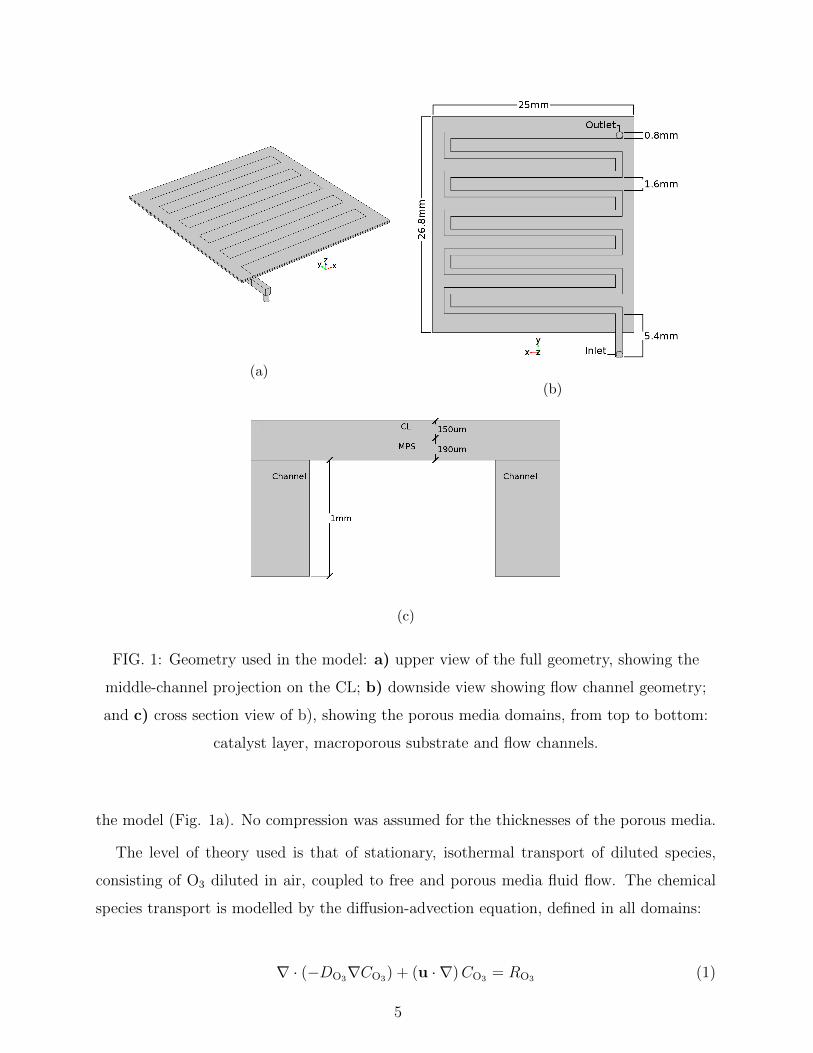
The geometry used for the simulations follows the one reported for the experimental

apparatus [6], and is presented in Figure 1: a single-channel serpentine geometry was used

for the flow field; a porous layer for the diffusion media, representing the macroporous carbon

paper substrate (MPS); and finally a silica gel based catalytic layer (CL), where the catalyst

is assumed homogeneously distributed. The CL includes a surface that follows the middle

of the flow channel projection, crossing the entire CL domain thickness, used for probing

4

(a)(b)

(c)

FIG. 1: Geometry used in the model: a) upper view of the full geometry, showing the

middle-channel projection on the CL; b) downside view showing flow channel geometry;

and c) cross section view of b), showing the porous media domains, from top to bottom:

catalyst layer, macroporous substrate and flow channels.

the model (Fig. 1a). No compression was assumed for the thicknesses of the porous media.

The level of theory used is that of stationary, isothermal transport of diluted species,

consisting of O3 diluted in air, coupled to free and porous media fluid flow. The chemical

species transport is modelled by the diffusion-advection equation, defined in all domains:

∇ · (−DO3∇CO3) + (u · ∇)CO3 = RO3 (1)

5

along with the definition of the species flux vector:

NO3 = −DO3∇CO3 + uCO3 (2)

Here, D is the diffusion coefficient of the species, C is the concentration, u is the flow velocity

vector, and R is the total reaction, source or sink, term. Since a dilute mixture is assumed,

the diffusion is given by Fick’s law.

The momentum transport follows three major mathematical frameworks: i) Stokes-Darcy

(SD), ii) Darcy-Brinkman (DB), or a mixed iii) Stokes-Brinkman (SB) formulation. The SD

approach consists of the compressible formulation of the Navier-Stokes equation:

ρ (u · ∇) u = ∇ ·[−P I + µ

(∇u + (∇u)T

)− 2

3µ (∇ · u) I

](3)

defined in the flow channel domain, and Darcy’s law:

u = −κµ∇P (4)

for the porous media domains. Here, ρ is the density of the fluid, P is the pressure, µ is the

viscosity of the fluid, κ is the porous medium permeability, and I is the identity matrix. It

should be noted that for Darcy’s law, the velocity u is actually given by the Darcy velocity,

which corresponds to the discharge rate per unit area. The DB formulation consists of a

single equation, defined in all domains:

ρ

ε(u · ∇)

(u

ε

)= ∇ ·

[−P I +

µ

ε

(∇u + (∇u)T

)− 2µ

3ε(∇ · u) I

]− µ

κu (5)

where ε is the porosity. The SB approach consists of using the Navier-Stokes equation for free

flow, while using Eq. 5 solely for the porous media domains. Regardless of the formulation

used, the continuity equation is also defined on all domains:

∇ · (ρu) = 0 (6)

where no momentum source or sink terms were used.

The full dilute species transport includes an inflow and outflow conditions at the inlet

and outlet, respectively (Fig. 1b). The effective diffusion coefficient, in the porous layers

domains, was given by:

Deff = feffD (7)

6

where feff was calculated using the tortuosity model feff = ε/τ , in the MPS; and the Brugge-

man model feff = ε3/2, for the CL. The reaction term in Equation 1 was defined for the O3

in the CL, representing the 1st-order reaction with the catalyst:

RO3 = −kCO3 (8)

where k is the apparent reaction rate constant. A no-flux condition was used in all re-

maining, outer surfaces, and the initial values for the O3, in all domains, follows the inflow

concentration of 1200 ppm.

For the momentum transport, the density and viscosity were assumed to be the same

as dry air at T = 298 K, neglecting the presence of O3. The porous layers are assumed

isotropic, and are characterized using the porosity and permeability of the material. The

inlet condition was given by a normal inflow velocity, defined by the flow rate, Q, over the

inlet area Ain:

u · n = Q/Ain (9)

with n being the vector normal to the inlet surface, andQ ranging from 200 to 450 cm3 min−1.

The outlet was defined by a constant pressure, with suppression of backflow, the value of it

being supplied by the authors of reference [6]. To allow comparison with different systems,

the Reynolds number was calculated using Q, the average kinematic viscosity over the entire

flow channel domain, and the hydraulic diameter for rectangular channels, assuming the

MPS as a solid wall. The remaining surfaces were all subjected to a no-slip condition. The

initial values used were u = 0 and P = 0.01 bar, and all simulations were subjected to a

reference pressure Pref , provided by the authors of [6].

For the SD and SB formulations, several setups were tested in order to implement the

interface boundary conditions described in [11]. Litte or no difference were seen when com-

paring the setups (Figs. S1-S4). The chosen setups, for comparison with the DB formulation,

includes a slip velocity for the free flow field at the interface between the channel and MPS

domains:

u =Ls

µτn,t (10)

where Ls is the slip length, and τn,t is the tangential shear stress at the boundary. The slip

length is given by the following[11]:

Ls = c

√κ

ε(11)

7

where c is an adjustable constant, taken as unity in this case. For the MPS domain, unlike

the proposed continuity condition for the flow field given in [11], only the pressure resulting

from the free flow in the interface was considered in either formulation. This is same as

the interpretation of the Beavers and Joseph interfacial condition given by Le Bars and

Worster[11]. The remaining setups investigated for the SD and SB formulations are described

in the Supplementary Information (SI)

The parameters used for the simulations are specified in Table I. Not all were available, for

instance the physical properties for the CL, which were estimated as follow: data regarding

the size distribution of the silica particles used were taken from the manufacturer (Nano Silica

Gel, Sigma Aldrich), reported to be between 6.0 and 9.0 µm, and then used in a simulation

of a permeability experiment to estimate the porosity and permeability: spherical particles,

with the mentioned particle range, were randomly distributed in a 1 mm width, 150 µm

thick, bidimensional bed, without superposition, and subjected to a flow with Reynolds

number ranging from 0.1 to 1. The bed pressure drop, assumed linear, was plotted against

the total discharge rate, and then fitted to the Darcy-Forchheimer equation[18] to provide

the permeability, where the porosity was evaluated from the void area in the bed. The

procedure was repeated 10 times, and the values reported in Table I are the average values.

Also not available was the reaction rate constant for the O3 reaction with the catalyst used

in the experiments (7-diethylamino-4-methylcoumarin[6]):

O3 + (C2H5)2 NC9H6O2CH3 → Products + hν (12)

It was, therefore, varied between 101 and 103 s−1, and chosen to better describe, qualitatively,

the partial pressure surfaces reported by Lopes et al. (Fig. 5 of [6]).

Finally, the mesh used for the computations was generated using a predefined “finer”

triangular mesh on all outer surfaces (min. and max. element sizes 3.06× 10−5 and 2.83×

10−4 m, respectively; max. element growth rate 1.1; curvature factor 0.4; and resolution

in narrow regions 0.9), with corner refinement (element size scaling factor 0.35), and the

domains were filled with a “coarse” tetrahedral mesh (min. and max. element sizes 2.29×

10−4 and 7.65 × 10−4 m, respectively; max. element growth rate 1.2; curvature factor 0.7;

and resolution in narrow regions 0.7), with 3 quadrilateral elements being included in the

direction normal to the flow channels walls (“boundary layer” elements). The final mesh

has element sizes ranging from 2.03 × 10−5 to 3.45 × 10−4 m, with an average element

8

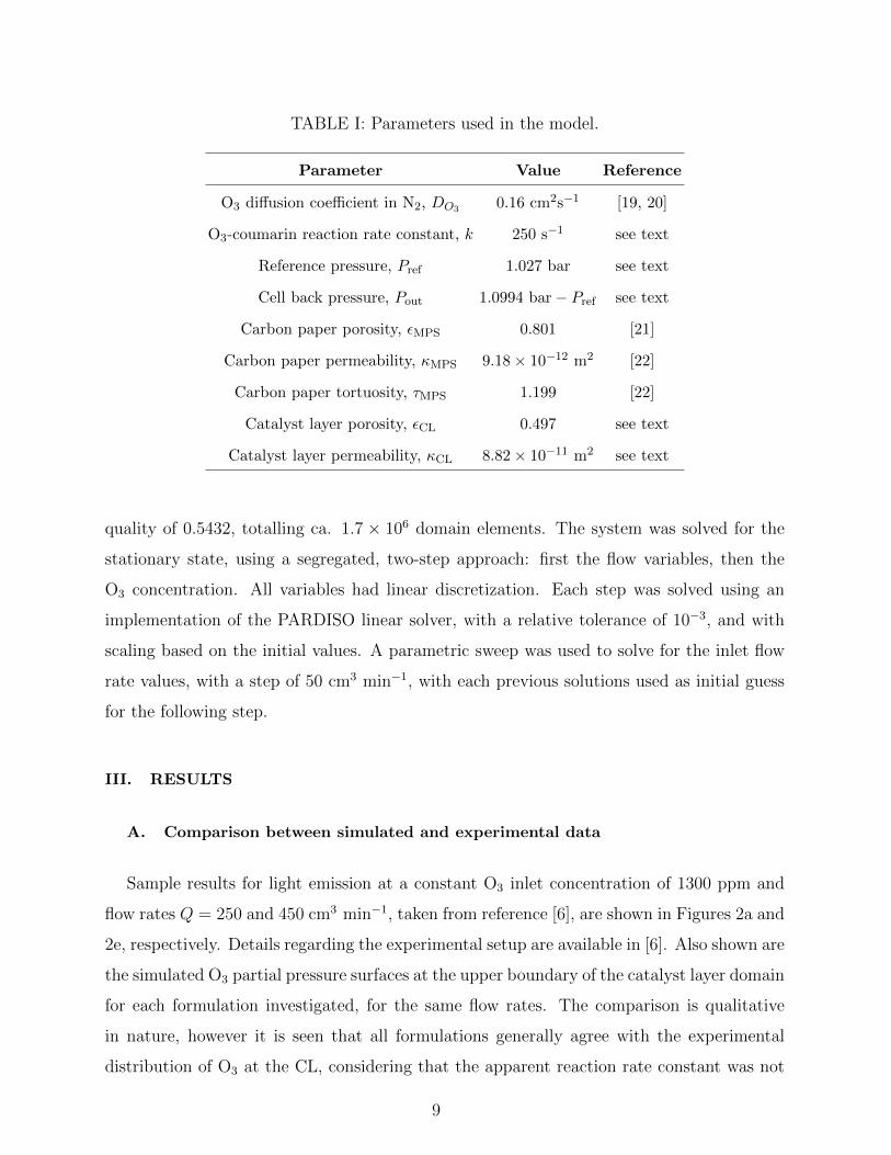
TABLE I: Parameters used in the model.

Parameter Value Reference

O3 diffusion coefficient in N2, DO3 0.16 cm2s−1 [19, 20]

O3-coumarin reaction rate constant, k 250 s−1 see text

Reference pressure, Pref 1.027 bar see text

Cell back pressure, Pout 1.0994 bar− Pref see text

Carbon paper porosity, εMPS 0.801 [21]

Carbon paper permeability, κMPS 9.18× 10−12 m2 [22]

Carbon paper tortuosity, τMPS 1.199 [22]

Catalyst layer porosity, εCL 0.497 see text

Catalyst layer permeability, κCL 8.82× 10−11 m2 see text

quality of 0.5432, totalling ca. 1.7 × 106 domain elements. The system was solved for the

stationary state, using a segregated, two-step approach: first the flow variables, then the

O3 concentration. All variables had linear discretization. Each step was solved using an

implementation of the PARDISO linear solver, with a relative tolerance of 10−3, and with

scaling based on the initial values. A parametric sweep was used to solve for the inlet flow

rate values, with a step of 50 cm3 min−1, with each previous solutions used as initial guess

for the following step.

III. RESULTS

A. Comparison between simulated and experimental data

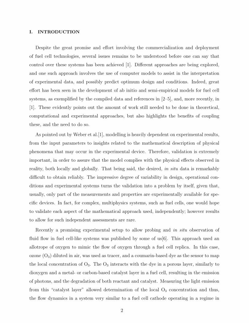
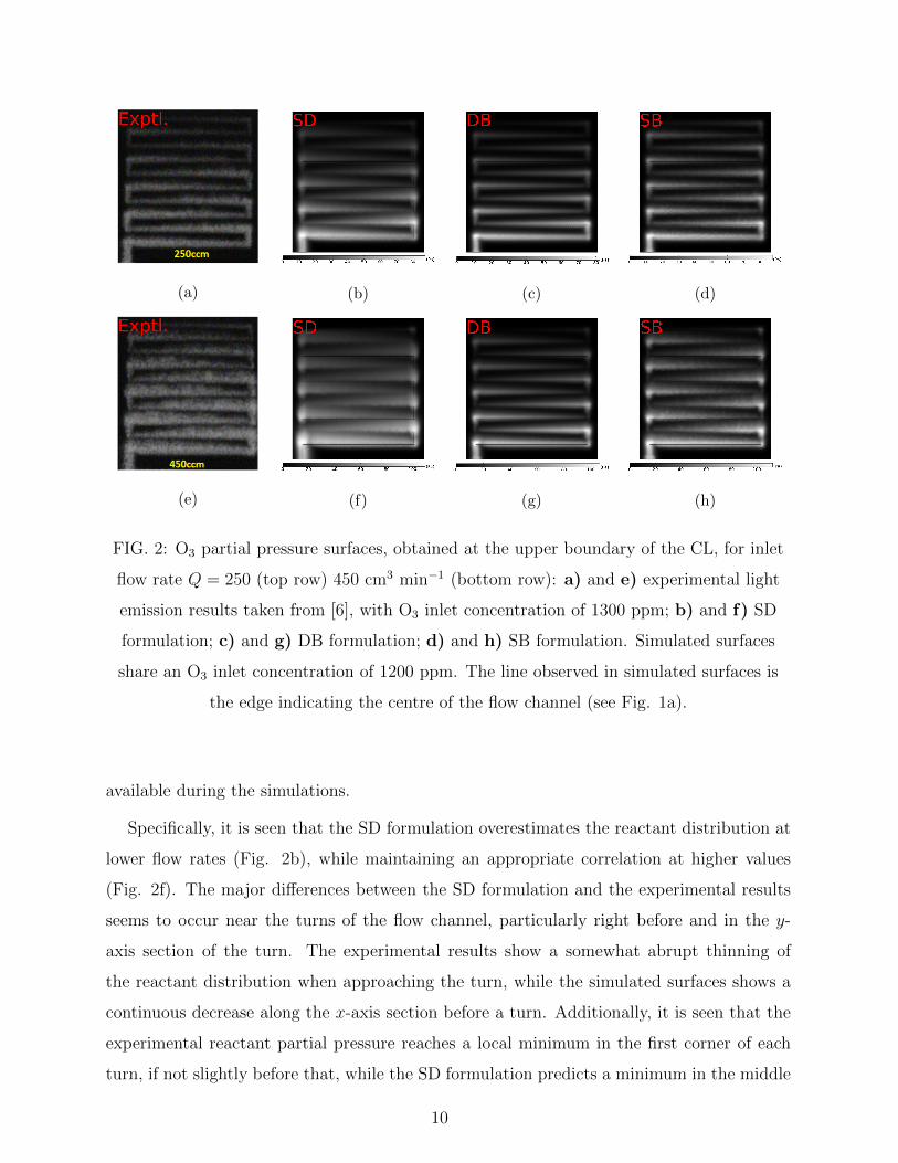
Sample results for light emission at a constant O3 inlet concentration of 1300 ppm and

flow rates Q = 250 and 450 cm3 min−1, taken from reference [6], are shown in Figures 2a and

2e, respectively. Details regarding the experimental setup are available in [6]. Also shown are

the simulated O3 partial pressure surfaces at the upper boundary of the catalyst layer domain

for each formulation investigated, for the same flow rates. The comparison is qualitative

in nature, however it is seen that all formulations generally agree with the experimental

distribution of O3 at the CL, considering that the apparent reaction rate constant was not

9

(a) (b) (c) (d)

(e) (f) (g) (h)

FIG. 2: O3 partial pressure surfaces, obtained at the upper boundary of the CL, for inlet

flow rate Q = 250 (top row) 450 cm3 min−1 (bottom row): a) and e) experimental light

emission results taken from [6], with O3 inlet concentration of 1300 ppm; b) and f) SD

formulation; c) and g) DB formulation; d) and h) SB formulation. Simulated surfaces

share an O3 inlet concentration of 1200 ppm. The line observed in simulated surfaces is

the edge indicating the centre of the flow channel (see Fig. 1a).

available during the simulations.

Specifically, it is seen that the SD formulation overestimates the reactant distribution at

lower flow rates (Fig. 2b), while maintaining an appropriate correlation at higher values

(Fig. 2f). The major differences between the SD formulation and the experimental results

seems to occur near the turns of the flow channel, particularly right before and in the y-

axis section of the turn. The experimental results show a somewhat abrupt thinning of

the reactant distribution when approaching the turn, while the simulated surfaces shows a

continuous decrease along the x-axis section before a turn. Additionally, it is seen that the

experimental reactant partial pressure reaches a local minimum in the first corner of each

turn, if not slightly before that, while the SD formulation predicts a minimum in the middle

10

of the y-axis section. This is observed even in the first turn, which has no contribution from

the crossing of reactant from the previous turns, which suggests it is an effect of the flow

field rather than the choice of reaction rate constant.

The DB and SB formulations predict similar surfaces for the O3 partial pressure distri-

bution to each other, particularly at low flow rates (Figs. 2c and 2d respectively). Similarly

to the SD formulation, the thinning of the reactant distribution along the x-axis sections of

the channel happens continuously, albeit in lesser extent due to a reduced distribution when

compared to the SD formulation. On the other hand, both surfaces show local reactant par-

tial pressure minima near the beginning of each turn, closely resembling the experimental

results. When comparing the two formulations, it is seen that the SB formulation shows

a larger amount of reactant crossing between turns than the DB one at higher flow rates

(Figs. 2h and 2g respectively), however this might be due to the choice of the reaction rate

constant.

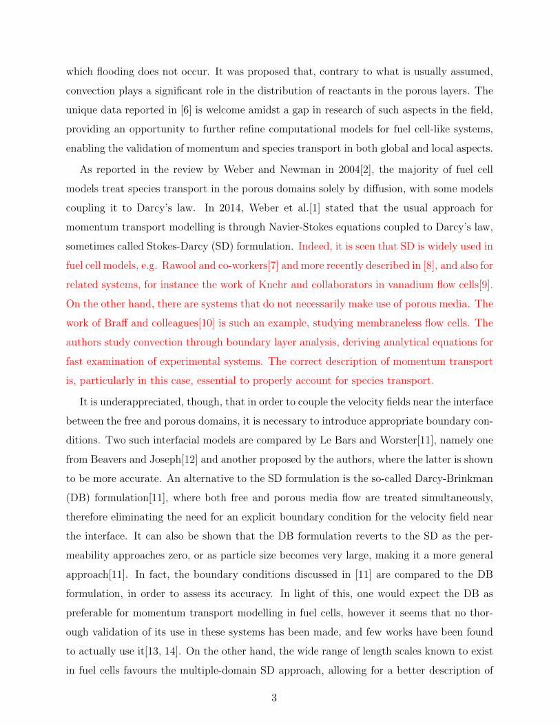
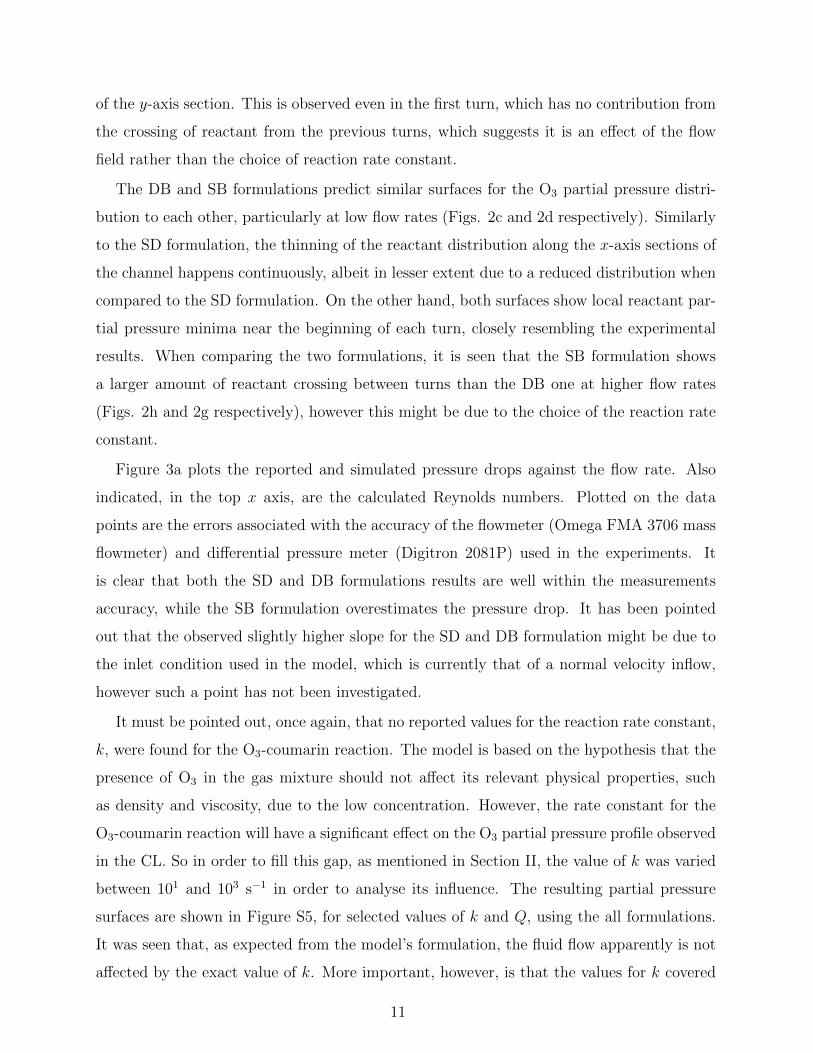
Figure 3a plots the reported and simulated pressure drops against the flow rate. Also

indicated, in the top x axis, are the calculated Reynolds numbers. Plotted on the data

points are the errors associated with the accuracy of the flowmeter (Omega FMA 3706 mass

flowmeter) and differential pressure meter (Digitron 2081P) used in the experiments. It

is clear that both the SD and DB formulations results are well within the measurements

accuracy, while the SB formulation overestimates the pressure drop. It has been pointed

out that the observed slightly higher slope for the SD and DB formulation might be due to

the inlet condition used in the model, which is currently that of a normal velocity inflow,

however such a point has not been investigated.

It must be pointed out, once again, that no reported values for the reaction rate constant,

k, were found for the O3-coumarin reaction. The model is based on the hypothesis that the

presence of O3 in the gas mixture should not affect its relevant physical properties, such

as density and viscosity, due to the low concentration. However, the rate constant for the

O3-coumarin reaction will have a significant effect on the O3 partial pressure profile observed

in the CL. So in order to fill this gap, as mentioned in Section II, the value of k was varied

between 101 and 103 s−1 in order to analyse its influence. The resulting partial pressure

surfaces are shown in Figure S5, for selected values of k and Q, using the all formulations.

It was seen that, as expected from the model’s formulation, the fluid flow apparently is not

affected by the exact value of k. More important, however, is that the values for k covered

11

260 325 391 457 523 590Reynolds Number

150 200 250 300 350 400 450 500500

1000

1500

2000

2500

3000

3500

4000

4500

Flow Rate (cm 3 min−1)

Pre

ssur

e D

rop

(Pa)

(a)

260 325 391 457 523 590Reynolds Number

150 200 250 300 350 400 450 500600

650

700

750

800

850

900

950

1000

1050

1100

Flow Rate (cm 3 min−1)

∆O3 (

ppm

)

(b)

FIG. 3: Global variables as a function of the inlet flow rate, simulated using SD (�), DB

(4) and SB (�) formulations, and the reported measured ones (◦). a) Pressure drop,

where the error bars represent uncertainty in the measurements. b) Total O3 consumption,

where the error bars represent one standard deviation in the measurements.

in this analysis seems to range from an underestimation to a large overestimation of the

reaction rate, at least given the remaining parameters and the comparison to the reported

experimental partial pressure surfaces[6]. An in-depth analysis of the best value of k is given

below.

The values of total O3 consumption for the experimental system, not published in refer-

ence [6], have also been used. Figure 3b presents the measured total reactant consumption

as a function of inlet flow rate, along with the simulated data for each formulation. All sim-

ulated values are statistically different from the measured values, although the SD and DB

results closely follows the measured values, with the SB formulation presenting a striking

deviation from the experimental data. This analysis suggests that, between the SD and DB

formulations, the SD is a better fit to the experimental data. Indeed, the mean absolute

and maximum errors calculated are, respectively, 25.37 and 31.77 for the SD, and 37.04

and 44.14 ppm for the DB formulation. However, since the total reactant consumption is

strongly dependent on the value of the reaction rate constant, such information is unreliable,

12

as the reaction rate constant may be independently adjusted in order to obtain close quanti-

tative agreement with the experimental values. Therefore, one must turn to the qualitative

behaviour of the response for each formulation. Figure S6 shows a shifted version of Figure

3b, where the simulated datasets have been shifted such that the first data point for all

datasets overlay. Such an approach makes explicit the differences in behaviour between the

predictions of each formulation, where it is clear that the slower decline in consumption pre-

dicted by the DB formulation more closely agrees with the experimental data. Additionally,

the Pearson correlation coefficient was calculated, resulting in 0.9688, 0.9856 and 0.9776 for

the SD, DB and SB formulations, respectively. This may be taken as indication that the DB

formulation may lead to a better predictor for the experimental data, albeit only slightly

more so than the other two.

In order to show that the choice of the reaction rate constant is not a major influence on

the behaviour of the ∆O3 = ∆O3(Q) curve, Figure S7 presents additional curves for selected

values of the reaction rate constant for each formulation. Some effect of k is observed for high

Q values, however it should be noticed that the values of k spans one order of magnitude.

Therefore it should be safe to conclude that the influence of the value of k on the behaviour

of the curve is weak.

Finally, a closer look at the concentration profiles was attempted. The normalized partial

pressure for O3 was evaluated along the edge present on the upper boundary of the CL, and

is shown in Figure 4 for the inlet flow rate of 350 cm3 min−1. The inset shows the full

simulated surface using the DB formulation and the edge used for evaluation of the data.

Also shown is the average of the two center pixels from the experimental results, supplied by

the authors of reference [6], roughly along the same path. The experimental data was filtered

in order to reduce noise, using a custom lowpass filter (order 5, density factor 20, passband

frequency 10 Hz, stopband frequency 100 Hz, sampling frequency 500 Hz, passband weight 1,

stopband weight 5). The data was normalized to its respective maximum value of O3 partial

pressure at the surface. It is clear from the inset, and the respective coloured sections in

the graph, that the spikes in partial pressure represent the second corner of each turn, while

the first spike represents the corner after the inlet. As expected from the general shape of

the reactant distribution surfaces shown in Figure 1, all formulations reproduce the general

behaviour of the experimental data, mainly the decay and said spikes in partial pressure, and

overestimate the near-entrance values. Upon closer inspection, it can be seen that the SD

13

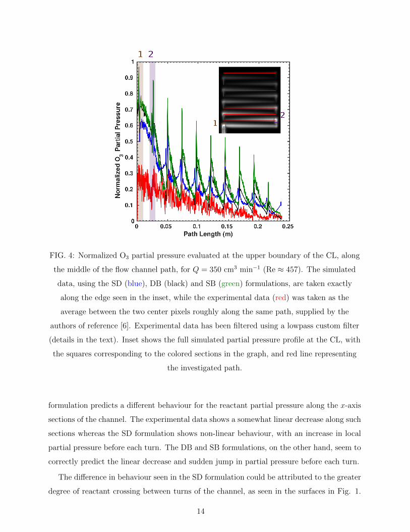
FIG. 4: Normalized O3 partial pressure evaluated at the upper boundary of the CL, along

the middle of the flow channel path, for Q = 350 cm3 min−1 (Re ≈ 457). The simulated

data, using the SD (blue), DB (black) and SB (green) formulations, are taken exactly

along the edge seen in the inset, while the experimental data (red) was taken as the

average between the two center pixels roughly along the same path, supplied by the

authors of reference [6]. Experimental data has been filtered using a lowpass custom filter

(details in the text). Inset shows the full simulated partial pressure profile at the CL, with

the squares corresponding to the colored sections in the graph, and red line representing

the investigated path.

formulation predicts a different behaviour for the reactant partial pressure along the x-axis

sections of the channel. The experimental data shows a somewhat linear decrease along such

sections whereas the SD formulation shows non-linear behaviour, with an increase in local

partial pressure before each turn. The DB and SB formulations, on the other hand, seem to

correctly predict the linear decrease and sudden jump in partial pressure before each turn.

The difference in behaviour seen in the SD formulation could be attributed to the greater

degree of reactant crossing between turns of the channel, as seen in the surfaces in Fig. 1.

14

In fact, when using different values of Q and k, such effect is also observed to a lesser extent

in the other formulations, being particularly weak in the DB formulation (see Fig. S8). It

was seen that the effect of the choice of k in the behaviour of the curve is relatively small,

as is in the total reactant consumption. For instance, in order to more closely correlate the

SD formulation to the experimental data, a reaction rate of 500 s−1 for low values of Q was

needed. However, as is shown in Figures S5 and S7, this would lead to an underestimation

of reactant distribution and overestimation of total reactant consumption. This constraint

points to an effect of the SD formulation’s resulting flow field, and not of the particular

choice of k.

B. Comparison between fluid flow formulations

Given the results and comparisons made above, some points can be drawn with respect to

the formulations investigated. Firstly, considering the parametrization described in Section

II, it is seen that the SD and DB formulations both generally agrees with the experimental

results, showing both good qualitative, and when possible quantitative, correlation. The

SB formulation, on the other hand, showed suitable qualitative results, particularly for the

spatial distribution of reactant in the CL (Fig. 2), however failed to give correct predictions

in the pressure drops and the behaviour of the reactant consumption curve (Figs 3a and

3b, respectively). Between the SD and DB formulations, the preference would arise from

the importance given to each qualitative comparison made, namely the spatial reactant

distribution and the partial pressure behaviour along the channel path (Fig. 4). On the

other hand, since the number of variables in the SD formulation is smaller, and the different

scales of a system are treated separately, it could be argued that the SD formulation is a

better choice, being computationally cheaper and as capable as the DB formulation.

Secondly, considering the constraints that emerged from the analysis of the reaction

rate constant, another perspective emerges. It stands that the SB formulation is still infe-

rior, given that the necessary value of k for an adequate reproduction of the total reactant

consumption would be greater than 500 s−1 (Fig. S7), but that would lead to a great un-

derestimation of the spatial distribution of reactant in the CL, even for high values of Q

(Fig. S5i). Even so, the behaviour of the total reaction consumption curve would still be

inadequate (Fig. S6), predicting a faster decline in consumption as a function of Q than the

15

experimental data. For the SD formulation, a similar situation is seen, in which different

values of k would be needed to fit the lower and higher Q sections of the reactant consump-

tion curve, albeit only slightly different from the chosen value of 250 s−1. However, it is

seen that the behaviour of the partial pressure along the channel path differs significantly

from the experimental data for such values (Fig. 4), and that values higher than 500 s−1

would be needed to minimize such differences (Fig. S8). This, in turn, would also lead to

a major underestimation of the reactant distribution in the CL (Fig. S5c). Finally, the DB

formulation appears to predict an adequate behaviour for the reactant consumption curve,

indicating the need of a slightly smaller value for k to actually fit the entire range of Q

investigated. Contrary to the other formulations, this would not lead to problems with the

remaining data, as the reactant distribution and partial pressure along the channel path are

already very close to the experimental data available.

It might be worthwhile, now, to take a closer look at the mathematical framework of the

formulations investigated. It has been shown that Eq. 4 can be derived from the Stokes

equation using the volume-averaging method[23]. Due to the constraints arising from length

scales during the derivation of Darcy’s law in [23], and the fact that the Stokes equation

is suitable for creeping flow, one obtains an equations that does not describes inertial or

viscous effects. This is readily seen when comparing Eqs. 4 and 3. The DB formulation,

Eq. 5, on the other hand, has been derived directly from the Navier-Stokes equations[11],

also using the volume-averaging method, while Ochoa-Tapia and Whitaker[24] show that

the so-called Brinkman corrections, present in Eq. 5, can be derived similarly to Darcy’s

law, i.e. from the Stokes equation. A major difference between the derivation of Eqs. 4

and 5 is that the latter is derived with no length scale constraints, which enables the single

equation approach mentioned in Section I, since Eq. 5 is valid in all domains throughout

the derivation[11, 24]. It should also be noticed that, as shown in [11], Eq. 4 is recovered by

taking the low permeability, or large particle diameter, limit of Eq. 5. This corroborates the

more general approach given by Eq. 5, despite the approximations used in its derivation.

Taking these into account, it has been mentioned that the lack of viscous effects in Eq. 4

leads to a poor treatment of the interfacial region between free and porous media flow[11, 24],

hence the need to modify Darcy’s law behaviour using slip conditions or by extending the

domain of validity of the Navier-Stokes equation[11] at the interface. It was discussed in

[11] that an appropriate boundary condition in the SD formulation gives good agreement

16

to the DB formulation, and that the differences scales with the Darcy number Da = κ/L2,

where the characteristic length L is usually taken as a slab of the porous medium, in this

case 190 µm. This would imply a small influence of the free flow field in the porous medium,

described by the thickness of a viscous transition zone δ =√

Da/ε ≈ 0.02. This is an

indicative of how deep the free flow field penetrates the porous medium, as predicted by the

full DB formulation, amounting to approximately the depth at which there is an exponential

decrease of the flow field with increasing depth. Hence, the SD formulation should be a good

approximation, when coupled to a proper description of the interface. However, a derivation

of Darcy’s law by Whitaker[23] suggests that the characteristic length might be taken from

a representative region of the medium, not necessarily the entirety of the slab. From X-ray

microtomography of a similar medium depicted here[21], it can be argued that the length

of such a region would be of ∼ 50 µm. This leads to a value of δ′ ≈ 0.07, and considering

the exponential decrease of the free flow field, a larger extent is expected, as exemplified in

[11]. Larger errors are expected, then, when using the SD formulation over DB, as shown

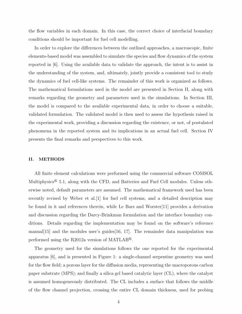
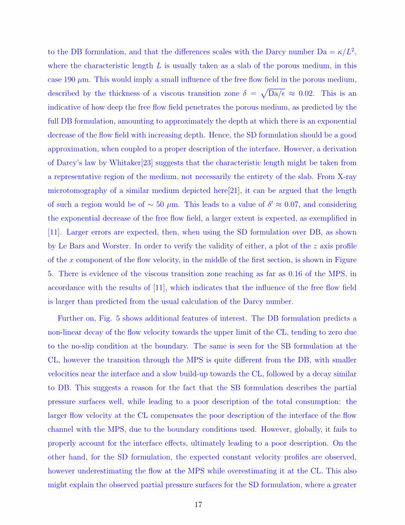
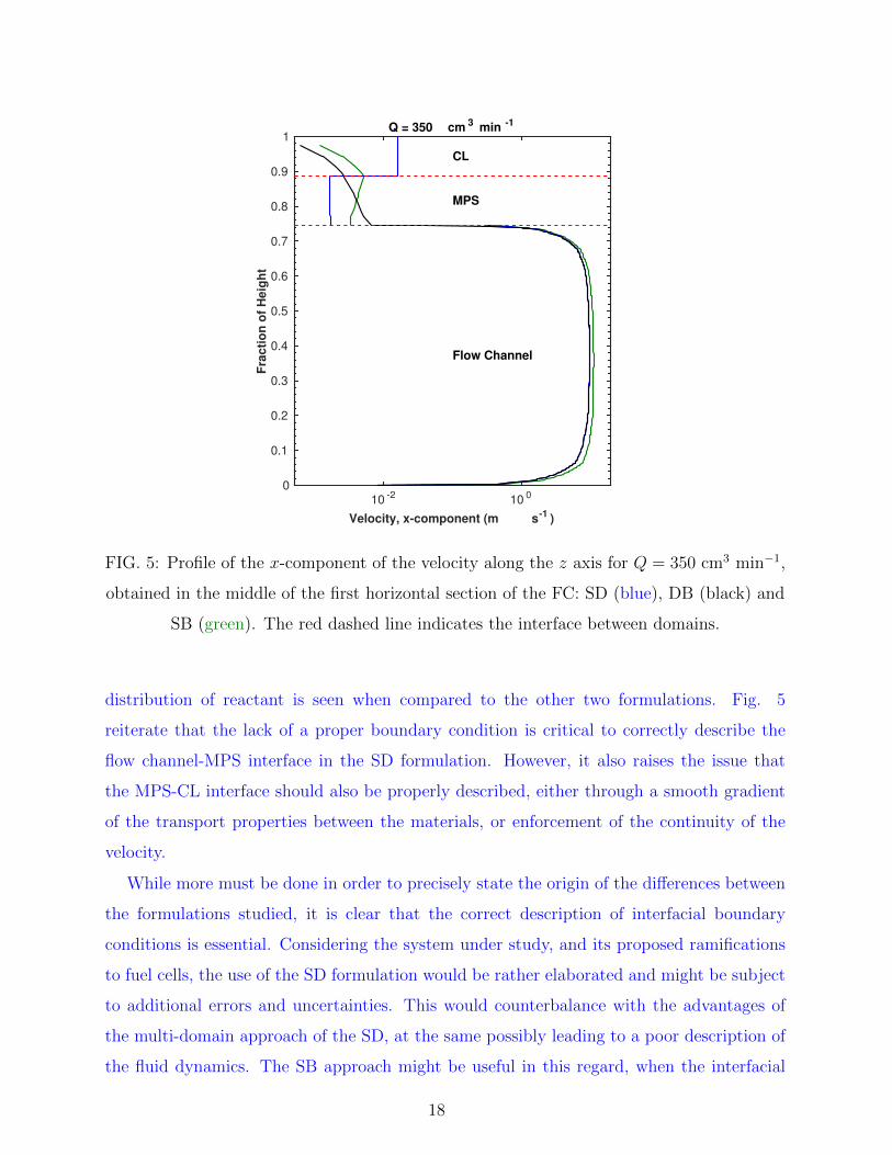
by Le Bars and Worster. In order to verify the validity of either, a plot of the z axis profile

of the x component of the flow velocity, in the middle of the first section, is shown in Figure

5. There is evidence of the viscous transition zone reaching as far as 0.16 of the MPS, in

accordance with the results of [11], which indicates that the influence of the free flow field

is larger than predicted from the usual calculation of the Darcy number.

Further on, Fig. 5 shows additional features of interest. The DB formulation predicts a

non-linear decay of the flow velocity towards the upper limit of the CL, tending to zero due

to the no-slip condition at the boundary. The same is seen for the SB formulation at the

CL, however the transition through the MPS is quite different from the DB, with smaller

velocities near the interface and a slow build-up towards the CL, followed by a decay similar

to DB. This suggests a reason for the fact that the SB formulation describes the partial

pressure surfaces well, while leading to a poor description of the total consumption: the

larger flow velocity at the CL compensates the poor description of the interface of the flow

channel with the MPS, due to the boundary conditions used. However, globally, it fails to

properly account for the interface effects, ultimately leading to a poor description. On the

other hand, for the SD formulation, the expected constant velocity profiles are observed,

however underestimating the flow at the MPS while overestimating it at the CL. This also

might explain the observed partial pressure surfaces for the SD formulation, where a greater

17

Velocity, x-component (m s-1 )

10-2

100

Fra

cti

on

of

He

igh

t

0

0.1

0.2

0.3

0.4

0.5

0.6

0.7

0.8

0.9

1

CL

MPS

Flow Channel

Q = 350 cm 3 min -1

FIG. 5: Profile of the x-component of the velocity along the z axis for Q = 350 cm3 min−1,

obtained in the middle of the first horizontal section of the FC: SD (blue), DB (black) and

SB (green). The red dashed line indicates the interface between domains.

distribution of reactant is seen when compared to the other two formulations. Fig. 5

reiterate that the lack of a proper boundary condition is critical to correctly describe the

flow channel-MPS interface in the SD formulation. However, it also raises the issue that

the MPS-CL interface should also be properly described, either through a smooth gradient

of the transport properties between the materials, or enforcement of the continuity of the

velocity.

While more must be done in order to precisely state the origin of the differences between

the formulations studied, it is clear that the correct description of interfacial boundary

conditions is essential. Considering the system under study, and its proposed ramifications

to fuel cells, the use of the SD formulation would be rather elaborated and might be subject

to additional errors and uncertainties. This would counterbalance with the advantages of

the multi-domain approach of the SD, at the same possibly leading to a poor description of

the fluid dynamics. The SB approach might be useful in this regard, when the interfacial

18

region is properly accounted for. However, similar difficulties would remain, and the fact

that the DB formulation in principle naturally accounts for these effects, tips the balance in

favor of the single-domain approach.

Considering the discussion above, and given the parametrization used and the constraints

observed in the simulated data to the experimental ones, the DB formulation is considered

more adequate to reproduce the behaviour of the system studied in [6], and more adequate

in its underlying assumptions to further study such system. Given the intended proximity

of this system to fuel cells, particularly devices based on polymer electrolyte membranes,

it is tempting to extend such conclusion to these devices. Care should be taken, however,

in extrapolating the presented results, as the model encompasses a rather limited range of

flow rates, and only consider the species transport of a diluted species. It is quite clear that,

as suggested by the authors of [6], the experimental technique developed, and the model

presented here, both are representative of the fluid flow in an air-operated fuel cell cathode.

However, for reacting mixtures as in fuel cell feeds, the diluted species approach breaks

down. Hence, for practical systems, the fluid and specially the species dynamics must be

carefully evaluated.

C. Implications for an actual fuel cell

In order to show what the results from Section III A would imply in an operating device,

a “polarization curve” was created from the models’ results. An analogy was drawn using

the mathematical framework of electrochemistry, avoiding the introduction of additional

variables and uncertainties through a non-validated electrochemical model. In the modelled

system, there are no activation or ohmic losses, hence it is not possible to simulate a full

polarization curve, as is commonly seen for fuel cells. The system is, on the other hand,

constantly under mass-transport limitation. Therefore, it is possible and worthwhile to look

at the differences in the concentration overpotential, ηC , given by the different models. It is

given by[25]

ηC = E − Eeq (13)

where E is the electrode potential for a given current, and Eeq is the electrode potential at

equilibrium, i.e. when no current is flowing. For the modelled system, this can be expressed

19

as

ηC =RT

Flog

(PO3

P ∗O3

)(14)

where R is the ideal gas constant; F is Faraday’s constant; PO3 is the local O3 partial

pressure in the CL domain (e.g. Fig. 2); and P ∗O3is the local O3 partial pressure in the

absence of reaction, i.e. disregarding Eq. 8 in the CL domain. Since the O3 partial pressure

is position-dependent, an average is taken over the CL domain, in order to facilitate analysis.

For the current, we consider Faraday’s law of electrolysis[25]:

I = FA∂CO3

∂t(15)

where A is the effective area for reaction at the CL domain. The right side of the equation

can be taken as the volume integral of FRO3 . In this way, the current is given by:

I = F

∫CL

RO3dV (16)

where the subscript denotes integration over the CL domain. Finally, taking the definition

of RO3 given by Eq. 8:

RO3 = −kCO3

it is noted that the “polarization” can be carried over by varying the reaction rate constant

k. The resulting curves for each model and selected inlet flow rates are shown in Figure 6.

It is noted that, as seen from the results of Section III A, both SD and SB formulations

overestimate reactant distribution, leading to significantly lower concentration overpoten-

tials for the same current value. No actual new information is shown in Fig. 6, however

the polarization curves sums up the observations presented and discussed before. That is,

relative to the best model shown, the DB formulation, the use of SD and SB formulations

tend to overestimate fuel cell performance. For instance, with Q = 350 cm3 min−1 and

k = 250 s−1, the results predicts currents ≈ 40% higher with an overpotential ≈ 15% lower,

for both SD and SB formulations relative to the DB one. For higher currents and flow rates,

the difference increases, most notably for the SB formulation. Therefore, it is expected that,

for commonly used flow rates and current ranges[26], the error associated with using the SD

formulation will only increase.

Also relevant to fuel cells is the treatment of multicomponent diffusion and the effects

of porous media. When the carrier fluid changes composition and is subject to pressure

20

0 0.1 0.2 0.3 0.4 0.5 0.6 0.7 0.8 0.9 1x 10−3

−0.14

−0.12

−0.1

−0.08

−0.06

−0.04

−0.02

0

Total Current (A)

Ave

rag

ed η

C (

V)

FIG. 6: Averaged concentration overpotential as a function of the total current, defined in

Eqs. 14 and 16, respectively, for SD (�), DB (4) and SB (�) formulations. Inlet flow rate

values contemplated: 250 (blue), 350 (red) and 450 cm3 min−1 (black).

gradients, different driving forces arise due to distinct interactions between the mixtures’

components. Meanwhile, when the mean free path of the components is comparable in

length to the medium’s pore size, collisions with the material become an important effect,

leading to the Knudsen regime of diffusion. It is well known that in practical devices,

such effects are important and must be taken into account[1], considering that the mixtures

are concentrated and change composition along the flow channel, and the mean free path

(λ ∼ 10−7 − 10−8 m [27]) and the pore size range of microporous layers used in actual fuel

cells (dp ∼ 10−7−10−8 m [28]). The Knudsen number, Kn = λ/L, is a useful indicator of the

prevalence of such regime, where in this case the characteristic length may be taken from the

average pore size. When Kn ∼ 1, as in the case described above, there is already significant

effects due to interactions with the porous material, increasing with Kn[29]. A recent work

by Fu and colleagues[30] shows the importance of a detailed treatment of diffusion using the

dusty gas model, which incorporates the Maxwell-Stefan model of multicomponent diffusion,

21

the Knudsen regime and pressure gradients. The author show that only by taking into

account these different physical processes, a good qualitative comparison with experimental

data can be achieved.

While the system under study is designed to be a replica of fuel cells, its conditions allow

for approximations to be used. As mentioned before, the use of a diluted, single species

diffusion may be justified by the fact that the carrier fluid does not change composition, and

the tracer concentration being quite low. Regarding Knudsen diffusion, the MPS typically

has a pore size range much larger than microporous layers (dMPS ∼ 10−5−10−6 m [31]), while

the CL used is very likely to be in a similar range, considering the particle size∼ 10−6 and the

transport properties obtained from simulations. These values gives Kn ≈ 7×10−3−7×10−2,

well bellow the value where molecular diffusion is expected to be significant, and slightly

smaller than the one that can be calculated from [30]. Nevertheless, some tests were carried

(see Section III of SI), using the Mixture-averaged model, with or without Knudsen diffusion,

and the Maxwell-Stefan model, all coupled to the DB formulation. Although not exactly

like the dusty gas model described in [30], it allows for an idea of the scale of these effects,

namely interspecies interactions, the Knudsen regime of diffusion and full pressure gradients.

Despite the approximations used for the relevant parameters, when compared to the diluted

approach, it is seen that the differences are small, specially when considering the degree of

freedom due to the reaction rate constant. More importantly, it is seem that the behaviour

of the curve is basically the same. This corroborates the approximations used in the model,

however it also shows that although the system described by Lopes and colleagues[6] can be

used to explore the flow field, it might be rather insensitive to higher order effects such as

the discussed above. Further improvements in the experimental setup and computational

model should allow the study of such effects.

D. Convective transport in the “gas diffusion layer”

Given the results presented in Section III A, and the discussion in Section III B, the DB

formulation was deemed more appropriate to evaluate the convective transport in the ex-

perimental system. Both qualitative and quantitative aspects investigated are appropriately

reproduced by the DB formulation, and the comparison with the SD and SB formulations

indicates that the main reasons for such success are a more suitable description of the bulk

22

fluid flow in porous medium and the continuity of the flow field near the interface between

free and porous medium domains.

We now turn to investigate the proposed contribution of convective transport for reactant

distribution in the CL, as reported in [6]. One point raised by Lopes et al. concerns the

contribution of secondary flows, in the form of vortices, to the distribution of reactants in

the catalyst layer, as have been previously suggested using laser Doppler anemometry in

an operating fuel cell[32]. Figure 7 presents the components of the velocity field in the

third turn of the flow channel for Q = 350 cm3 min−1 (Re ≈ 457), both in the xy and xz

planes. Each surface presents the component of the velocity perpendicular to the plane,

with the remaining components as streamlines. It is clear from the streamlines the existence

of secondary flows, in the form of vortices, and an offset of these velocity components from

the center of the flow channels. It is also seen the existence of circulation movement in the

turn, as seen in the xz cut, with an upflow of fluid in the upper part of the channel, closer to

the MPS, which is consistent to previous results[7]. The information in Figure 7 correlates

with the observed features in the partial pressure surfaces, experimental and simulated,

corroborating the idea that secondary flows are important to describe the observed reactant

spatial distribution[6].

Secondary flows are, of course, expected for non-ideal fluids and finite geometries, though

a main concern is the actual contribution to reactant distribution in a device. To investigate

this, simulations were performed using a modified model, where the species transport in the

porous media is uncoupled from the momentum transport, while still solving for the full

flow field, i.e. Eq. 1 becomes the diffusion equation:

∇ · (−DO3∇CO3) = RO3 (17)

in the porous media domains. Figure S9 presents the reactant distribution surfaces in the

CL. As expected, the reactant partial pressure in the CL is reduced when compared to the

full model (e.g. Fig. 2c), however somewhat constant, despite the increase in inlet flow

rate. The most striking result of the modified model is the loss of several features in the

reactant distribution when compared to the full model, particularly the ones seen closer to

the turns of the flow channel. This is better shown in Figure 8, where the difference between

the modified and full models’ partial pressure surfaces is presented for Q = 350 cm3 min−1.

The data was generated using a 536× 500 rectangular grid. Taking the partial pressure as

23

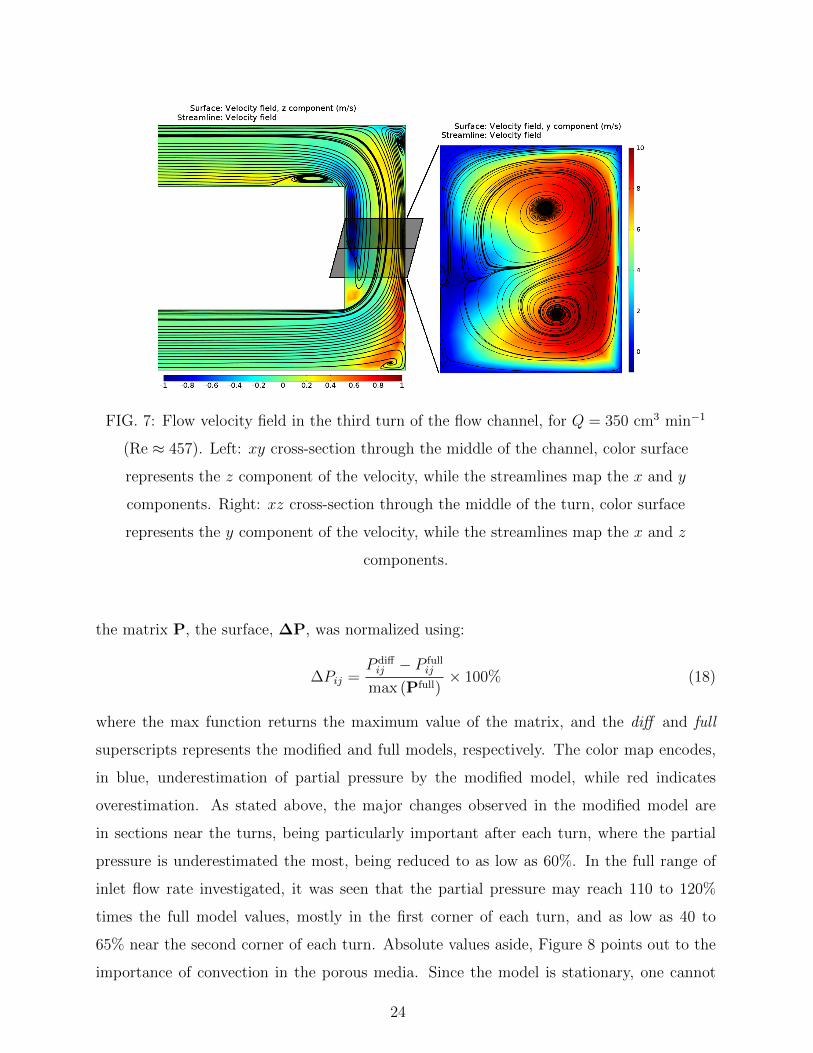
FIG. 7: Flow velocity field in the third turn of the flow channel, for Q = 350 cm3 min−1

(Re ≈ 457). Left: xy cross-section through the middle of the channel, color surface

represents the z component of the velocity, while the streamlines map the x and y

components. Right: xz cross-section through the middle of the turn, color surface

represents the y component of the velocity, while the streamlines map the x and z

components.

the matrix P, the surface, ∆P, was normalized using:

∆Pij =P diffij − P full

ij

max (Pfull)× 100% (18)

where the max function returns the maximum value of the matrix, and the diff and full

superscripts represents the modified and full models, respectively. The color map encodes,

in blue, underestimation of partial pressure by the modified model, while red indicates

overestimation. As stated above, the major changes observed in the modified model are

in sections near the turns, being particularly important after each turn, where the partial

pressure is underestimated the most, being reduced to as low as 60%. In the full range of

inlet flow rate investigated, it was seen that the partial pressure may reach 110 to 120%

times the full model values, mostly in the first corner of each turn, and as low as 40 to

65% near the second corner of each turn. Absolute values aside, Figure 8 points out to the

importance of convection in the porous media. Since the model is stationary, one cannot

24

FIG. 8: Normalized difference between the modified and full models’ partial pressure

surfaces for Q = 350 cm3 min−1 (Re ≈ 457): Blue represents underestimation of the partial

pressure by the modified model, while red represents overestimation. Normalization was

made using the maximum value at the full model’s surface (see. Eq. 18). The values were

taken in a 536× 500 grid, with uniform interval of 50 µm. Grey line represents the centre

of the flow channel.

claim that the underestimated effects are those resulting specifically from secondary flows,

such as seen in Figure 7, however, it is quite clear that the crossing of reactant between

horizontal sections and turns of the channel are mainly due to convection.

The information presented in Figures 7 and 8 correlates well with the interpretation

of Lopes et al. concerning the experimental results reported in [6]. It is proposed that

convection plays a significant part in the reactant distribution in the porous media, calling

for engineering not only flow channels, but also the so-called gas diffusion layers, to maximize

reactant distribution and, therefore, enhance device efficiency. In this line, an attempt was

performed to identify the contribution of convection in the experimental system. A change

of slope in the curve of light intensity, proportional to O3 partial pressure, as function of

25

inlet flow rate (Re ≈ 480) was identified as a saturation of convective transport in the

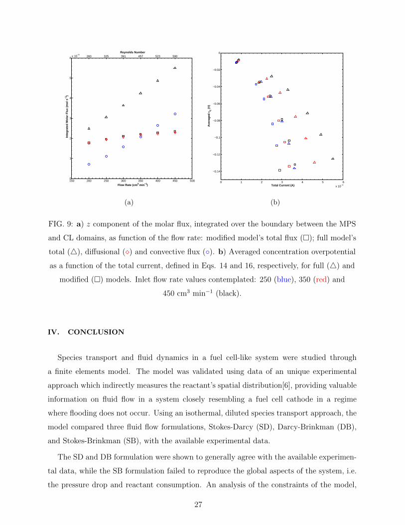
porous media[6]. To verify this, the contributions to the molar flux of reactant to the CL

were analysed. Figure 9a presents the z component of each contribution to the molar flux

(Eq. 2), integrated over the boundary between the MPS and CL domains, for both modified

and full models. It can be interpreted as the total amount of reactant transported to the

CL per unit time, and, as expected, the amount accounted in the full model is significantly

higher than that in the modified model. More importantly, though, is the fact that in both

models the diffusional contribution, being the total amount in the modified one, is the one

presenting an asymptotic behaviour, while the convective contribution, in the case of the full

model, increases almost linearly over the entire inlet flow rate range investigated. Therefore,

contrary to interpretation given in [6], the convective contribution to reactant transport

actually increases throughout the flow rate range (Re = 260 to 590), amounting from 29 to

58% of the total reactant transport to the CL.

Finally, the same approach of Section III C is used to sum up the implications of these

findings for an actual fuel cell. Figure 9b compares the “polarization curves” of the full and

diffusion-only models for selected values of inlet flow rate. It is seen that convection greatly

increases the current for similar overpotential values. In particular, for Q = 350 cm3 min−1,

the contribution of convection ranges from 8.9% to 26.9% for the total current, while de-

creasing the concentration overpotential from 26.2% to 3.3%. As seen in the Figure, this

contribution increases with Q, in the same way as seen in Fig. 9a, playing a significant role

in higher values of flow rate. For the range of Q and k simulated, this reaches as much as

34.0% of the current, with an overpotential 5.3% smaller.

In a sense, the behaviour of the diffusional contribution to the species transport is ex-

pected, given that it is driven by the gradient of the reactant’s partial pressure, which, in

turn, is connected to the catalyst’s turnover frequency. Hence, for a given catalyst and

operational conditions, the diffusional transport is bound to saturate. On the other hand,

the convective transport provides an almost independent contribution to the molar flux,

enabling a larger distribution of reactant in the porous media, as seen in Figures 8 and 9a,

for the same conditions. This reinforces the call for engineering of porous media as well as

flow channels, and adds to the possibilities of enhancing fuel cell efficiency by tuning not

only water management, but also catalyst distribution coupled to convective transport.

26

260 325 391 457 523 590Reynolds Number

150 200 250 300 350 400 450 5000

1

2

3

4

5

6x 10−9

Flow Rate (cm 3 min−1)

Inte

grat

ed M

olar

Flu

x (m

ol s

−1)

(a)

0 1 2 3 4 5 6x 10−4

−0.14

−0.12

−0.1

−0.08

−0.06

−0.04

−0.02

0

Total Current (A)

Ave

rag

ed η

C (

V)

(b)

FIG. 9: a) z component of the molar flux, integrated over the boundary between the MPS

and CL domains, as function of the flow rate: modified model’s total flux (�); full model’s

total (4), diffusional (�) and convective flux (◦). b) Averaged concentration overpotential

as a function of the total current, defined in Eqs. 14 and 16, respectively, for full (4) and

modified (�) models. Inlet flow rate values contemplated: 250 (blue), 350 (red) and

450 cm3 min−1 (black).

IV. CONCLUSION

Species transport and fluid dynamics in a fuel cell-like system were studied through

a finite elements model. The model was validated using data of an unique experimental

approach which indirectly measures the reactant’s spatial distribution[6], providing valuable

information on fluid flow in a system closely resembling a fuel cell cathode in a regime

where flooding does not occur. Using an isothermal, diluted species transport approach, the

model compared three fluid flow formulations, Stokes-Darcy (SD), Darcy-Brinkman (DB),

and Stokes-Brinkman (SB), with the available experimental data.

The SD and DB formulation were shown to generally agree with the available experimen-

tal data, while the SB formulation failed to reproduce the global aspects of the system, i.e.

the pressure drop and reactant consumption. An analysis of the constraints of the model,

27

regarding reactant distribution and total consumption, and description of the interface be-

tween the flow channel and porous media, led to the choice of the DB formulation as more

appropriate to describe the system. It must be noted that the SD formulation is currently

taken as the standard approach for fuel cell modelling[1], while the DB formulation seems

to lack a proper validation[11] and use in fuel cell modelling, despite having some physical

justification for its use. The results and comparison presented in Sections III A and III B

points to the necessity of better descriptions in the porous media flow of fuel cells, while

providing a semi-quantitative validation of the DB formulation in these systems.

The implication of the differences between formulations observed in Section III A were

briefly discussed in Section III C. A polarization curve analogy was used to compare the

concentration overpotential between the studied formulations. It was shown that both SD

and SB formulations overestimate fuel cell performance, relative to the DB one. The re-

sults shown suggest that the error of using simplified mathematical formulations, relative to

DB, are bound to increase when considering the usual range of flow rate and currents for

commercial fuel cell devices[26].

The validated model was then used to investigate remarks raised in the experimental

work[6]. It has been shown that uncoupling the momentum transfer in the porous media led

to a loss of several of the observed features in both experimental and simulated reactant’s

spatial distribution. This points out that secondary flows does indeed correlates with the

observed experimental and simulated phenomena. Furthermore, the results confirm the

assertion made in [6] that, contrary to what is usually assumed, convection provides a major

contribution to reactant distribution in the porous layers, from 29 to 58% of total reactant

transport to the catalyst layer, in a inlet flow rate range of 200 to 450 cm3 min−1 (channel

Re = 260 to 590). The diffusive transport shows an asymptotic dependence on the inlet

flow rate, while the convective transport shows an almost linear increase over the entire

range of flow rate. Using the same approach as in Section III C, it is shown that convection

significantly increases the current range for similar values of concentration overpotential,

reaching 34.0% higher current for 5.3% lower overpotential in the range of Q and k simulated.

More work needs to be done, though, in both experimental and computational approaches.

Some differences between the measurements are pointed out, and these can be related to the

approach used in the model, under or overestimating the physical processes, or to experi-

mental uncertainties. Therefore there is a need to refine both levels, to provide a rigorous

28

comparison between both approaches. In the computational level, electronic structure cal-

culations might provide powerful insights in the catalyst-reactant interaction, which, with

an improved mathematical formulation, might allow for accurate time dependent simula-

tions, enabling the identification of causal relations in the system. In the experimental level,

providing accurate values for the physical properties of the materials used, and exploring

the effects of different variables, such as the temperature, should allow for a more rigor-

ous comparison to the model. Improvements of the spatial resolution on both levels is also

highly desirable, since it should provide additional information on the finer scale effects that

contribute to the overall behaviour of the system. On the other hand, the current level does

provide some insights, and more studies, e.g. with different channel geometries, may already

lead to a solid representation and additional understanding of the system.

Ultimately, the coupling of experimental and computational efforts in modelling a more

complex system, in this case fuel cells, are intended to lead to a tool with the capabilities

of predicting and optimizing operational design and conditions in the full device.

ACKNOWLEDGMENTS

The authors are grateful to the referees for suggestions and pointing out mistakes, al-

lowing for the improvement of the manuscript. Beruski acknowledges a Ph.D. scholarship,

grant #2013/11316-9, from Sao Paulo Research Foundation (FAPESP). Beruski is grate-

ful to Dr. Manuel Cruz and Dr. Harry Schulz for discussions. Lopes acknowledges the

Centro Nacional de Desenvolvimento Cientıfico e Tecnologico (CNPq) for the post-Doc fel-

lowship, process #150249/2014-4. Kucernak acknowledges funding from the UK Engineering

and Physical Sciences research council under EP/G030995/1 –Supergen Fuel Cell Consor-

tium. Perez acknowledges grants #2011/50727-9 and #2013/16930-7, FAPESP, and grant

#311208/2015-0, CNPq.

A file containing the data used to generate the plots in this paper and in the suppementary

materials is available with the DOI:10.5281/zenodo.60642.

[1] A. Z. Weber, R. L. Borup, R. M. Darling, P. K. Das, T. J. Dursch, W. Gu, D. Harvey,

A. Kusoglu, S. Litster, M. M. Mench, R. Mukundan, J. P. Owejan, J. G. Pharoah, M. Secanell,

29

and I. V. Zenyuk. A critical review of modeling transport phenomena in polymer-electrolyte

fuel cells. J. Electrochem. Soc., 161:F1254–F1299, 2014.

[2] A. Z. Weber and J. Newman. Modeling transport in polymer-electrolyte fuel cells. Chem.

Rev., 104:4679–4726, 2004.

[3] C.-Y. Wang. Fundamental models for fuel cell engineering. Chem. Rev., 104:4727–4766, 2004.

[4] K.-D. Kreuer, S. J. Paddison, E. Spohr, and M. Schuster. Transport in proton conductors

for fuel-cell applications: simulations, elmentary reactions and phenomenology. Chem. Rev.,

104:4673–4678, 2004.

[5] M. Bavarian, M. Soroush, I. G. Kevrekidis, and J. B. Benziger. Mathematical modeling,

steady-state and dynamic behavior, and control of fuel cells: a review. Ind. Eng. Chem. Res.,

49:7922–7950, 2010.

[6] T. Lopes, M. Ho, B. K. Kakati, and A. R. J. Kucernak. Assessing the performance of reactant

transport layers and flow fields towards oxygen transport: A new imaging method based on

chemiluminescence. J. Power Sources, 274:382–392, 2015.

[7] A. S. Rawool, S. K. Mitra, and J. G. Pharoah. An investigation of convective transport in

micro proton-exchange membrane fuel cells. J. Power Sources, 162:985–991, 2006.

[8] F. Barbir. PEM fuel cells: thoery and practice. Academic Press, 225 Wyman Street, Waltham,

MA 02451, USA, 2nd edition, 2013.

[9] K. W. Knehr, E. Agar, C. R. Dennison, A. R. Kalidindi, and E. C. Kumbur. A transient

vanadium flow battery model incorporating vanadium crossover and water transport through

the membrane. J. Electrochem. Soc., 159:A1446–A1459, 2012.

[10] W. A. Braff, C. R. Buie, and M. Z. Bazant. Boundary layer analysis of membraneless electro-

chemical cells. J. Electrochem. Soc., 160:A2056–A2063, 2013.

[11] M. Le Bars and M. G. Worster. Interfacial conditions between pure fluid and a porous medium:

implications for binary alloy solidification. J. Fluid Mech., 550:149–173, 2006.

[12] G. S. Beavers and D. D. Joseph. Boundary conditions at a naturally permeable wall. J. Fluid.

Mech., 30:197–207, 1967.

[13] O. Razbani, M. Assadi, and M. Andersson. Three dimensional CFD modeling and experimen-

tal validation of an electrolyte supported solid oxide fuel cell fed with methane-free biogas.

Int. J. Hydrogen Energ., 38:10068–10080, 2013.

[14] L. Valino, R. Mustata, and L. Duenas. Consistent modeling of a single PEM fuel cell using

30

Onsager’s principle. Int. J. Hydrogen Energ., 39:4030–4036, 2014.

[15] COMSOL. COMSOL Multiphysics Reference Manual, 2015. Version 5.1.

[16] COMSOL. CFD Module User’s Guide, 2015. Version 5.1.

[17] COMSOL. Batteries & Fuel Cells Module User’s Guide, 2015. Version 5.1.

[18] V. Gurau, M. J. Bluemle, E. S. De Castro, Y.-M. Tsou, T. A. Zawodzinski Jr., and J. A.

Mann Jr. Characterization of transport properties in gas diffusion layers for proton exchange

membrane fuel cells 2. Absolute permeability. J. Power Sources, 165:793–802, 2007.

[19] R. Ono and T. Oda. Spatial distribution of ozone density in pulsed corona discharge s observed

by two-dimensional laser absorption method. J. Phys. D: Appl. Phys., 37:730–735, 2004.

[20] W. J. Massman. A review of the molecular diffusivities of H2O, CO2, CH4, CO, O3, SO2,

NH3, N2O, NO and NO2 in air, O2 and N2 near STP. Atmos. Environ., 32:1111–1127, 1998.

[21] Z. Fishman, J. Hinebaugh, and A. Bazylak. Microscale tomography investigations of het-

erogeneous porosity distributions of PEMFC GDLs. J. Electrochem. Soc., 157:B1643–B1650,

2010.

[22] Z. Fishman and A. Bazylak. Heterogeneous through-plane distributions of tortuosity, effective

diffusivity, and permeability for PEMFC GDLs. J. Electrochem. Soc., 158:B247–B252, 2011.

[23] S. Whitaker. Flow in porous media I: A theoretical derivation of Darcy’s law. Transport

Porous Med., 1:3–25, 1986.

[24] J. A. Ochoa-Tapia and S. Whitaker. Momentum transfer at the boundary between a porous

medium and a homogeneous fluid–I. Theoretical development. Int. J. Heat Mass Transfer,

38:2635–2646, 1995.

[25] A. J. Bard and L. R. Faulkner. Electrochemical Methods: Fundamentals and Applications.

John Wiley & Sons, 2nd edition, 2001.

[26] Single Cell Testing Task Force. Single cell test protocol. Technical Report 05-014B.2, US Fuel

Cell Council, 1100 H Street, NW, Suite 800, Washington, DC, July 2006.

[27] H. V. Kehiaian. Mean free path and related properties of gases. In J. R. Rumble, editor,

CRC Handbook of Chemistry and Physics, chapter Fluid Properties. CRC Press/Taylor and

Francis, Boca Raton, FL, 98th edition, (internet version) 2018.

[28] M. V. Williams, E. Begg, L. Bonville, H. R. Kunz, and J. M. Fenton. Characterization of gas

diffusion layers for PEMFC. J. Electrochem. Soc., 151:A1173–A1180, 2004.

[29] L. Wu. A slip model for rarified gas flows at arbitrary Knudsen number. Appl. Phys. Lett.,

31

93:253103, 2008.

[30] Y. Fu, J. Yi, S. Poizeau, A. Dutta, A. Mohanram, J. D. Pietras, and M. Z. Bazant. Multi-

component gas diffusion in porous electrodes. J. Electrochem. Soc., 162:F613–F621, 2015.

[31] S. Park, J.-W. Lee, and B. N. Popov. Effect of carbon loading in microporous layer on PEM

fuel cell performance. J. Power Sources, 163:357–363, 2006.

[32] C. Kalyvas, A. Kucernak, D. Brett, G. Hinds, S. Atkins, and N. Brandon. Spatially resolved

diagnostic methods for polymer electrolyte fuel cells: a review. WIREs Energy Environ.,

3:254–275, 2014.

32