Gas Dynamics and Large–Scale Morphology of the Milky … · Gas Dynamics and Large–Scale Morphology of the Milky Way Galaxy 3 Figure1.(l,v) diagram for 12CO from unpublished data

arX

iv:a

stro

-ph/

9810

208v

1 1

4 O

ct 1

998

Mon. Not. R. Astron. Soc. 000, 000–000 (0000) Printed 13 August 2013 (MN LATEX style file v1.4)

Gas Dynamics and Large–Scale Morphology of the Milky

Way Galaxy

Peter Englmaier and Ortwin Gerhard

13 August 2013

ABSTRACTWe present a new model for the gas dynamics in the galactic disk inside the Sun’s orbit.Quasi–equilibrium flow solutions are determined in the gravitational potential of thedeprojected COBE NIR bar and disk, complemented by a central cusp and, in somemodels, an outer halo. These models generically lead to four–armed spiral structurebetween corotation of the bar and the solar circle; their large–scale morphology is notsensitive to the precise value of the bar’s pattern speed, to the orientation of the barwith respect to the observer, and to whether or not the spiral arms carry mass.

Our best model provides a coherent interpretation of many observed gas dynamicalfeatures. Its four-armed spiral structure outside corotation reproduces quantitativelythe directions to the five main spiral arm tangents at |l| ≤ 60 observed in a variety oftracers. The 3-kpc-arm is identified with one of the model arms emanating from theends of the bar, extending into the corotation region. The model features an inner gasdisk with a cusped orbit shock transition to an x2 orbit disk of radius R ∼ 150 pc.

The bar’s corotation radius is fairly well–constrained at Rc ≃ 3.5 ± 0.5 kpc. Thebest value for the orientation angle of the bar is probably 20−25, but the uncertaintyis large since no detailed quantitative fit to all features in the observed (l, v) diagramsis yet possible. The Galactic terminal velocity curve from HI and CO observationsout to l ≃ ±45 (∼ 5 kpc) is approximately described by a maximal disk model withconstant mass–to–light ratio for the NIR bulge and disk.

Key words: Galaxy: structure, Galaxy: kinematics and dynamics, Galaxy: centre,Galaxies: spiral, Interstellar medium: kinematics and dynamics, Hydrodynamics.

1 INTRODUCTION

Although the Milky Way is in many ways the best stud-ied example of a disk galaxy, it has proven exceedingly dif-ficult to reliably determine its large–scale properties, suchas the overall morphology, the structural parameters of themain components, the spiral arm pattern, and the shape ofthe Galactic rotation curve. A large part of this difficultyis due to distance ambiguities and to the unfortunate lo-cation of the solar system within the Galactic dust layer,which obscures the stellar components of the Galaxy in theoptical wavebands. With the advent of comprehensive near–infrared observations by the COBE/DIRBE satellite andother ground- and space–based experiments, this situationhas improved dramatically. These data offer a new route tomapping out the Galaxy’s stellar components, to connect-ing their gravitational potential with the available gas andstellar kinematic observations, and thereby to understand-ing the large–scale structure and dynamics of the Milky WayGalaxy.

From radio and mm–observations it has long beenknown that the atomic and molecular gas in the inner

Galaxy does not move quietly on circular orbits: “forbidden”and non–circular motions in excess of 100 kms−1 are seenin longitude–velocity (l, v)–diagrams (e.g., Burton & Liszt1978, Dame et al. 1987, Bally et al. 1987). Some of the moreprominent features indicating non–circular motions are the3 kpc–arm, the molecular parallelogram (“expanding molec-ular ring”), and the unusually high central peak in the termi-nal velocity curve at l ≃ ±2. Many papers in the past havesuggested that these forbidden velocities are best explainedif one assumes that the gas moves on elliptical orbits in abarred gravitational potential (Peters 1975, Cohen & Few1976, Liszt & Burton 1980, Gerhard & Vietri 1986, Mulder& Liem 1986, Binney et al. 1991, Wada et al. 1994).

In the past few years, independent evidence for a barin the inner Galaxy has been mounting from NIR photome-try (Blitz & Spergel 1991, Weiland et al. 1994, Dwek et al.1995), from IRAS and clump giant source counts (Nakadaet al. 1991, Whitelock & Catchpole 1992, Nikolaev & Wein-berg 1997, Stanek et al. 1997), from the measured large mi-crolensing optical depth towards the bulge (Paczynski et al.1994, Zhao, Rich & Spergel 1996) and possibly also from

c© 0000 RAS

http://arxiv.org/abs/astro-ph/9810208v1

2 P. Englmaier and O.E. Gerhard

stellar kinematics (Zhao, Spergel & Rich 1994). See Gerhard(1996) and Kuijken (1996) for recent reviews.

The currently best models for the distribution of oldstars in the inner Galaxy are based on the NIR data fromthe DIRBE experiment on COBE. Because extinction is im-portant towards the Galactic nuclear bulge even at 2 µm,the DIRBE data must first be corrected (or ‘cleaned’) forthe effects of extinction. This has been done by Spergel,Malhotra & Blitz (1996), using a fully three-dimensionalmodel of the dust distribution (see also Freudenreich 1998).Binney, Gerhard & Spergel (1997, hereafter BGS) used aRichardson–Lucy algorithm to fit a non-parametric modelof j(r) to the cleaned data of Spergel et al. under the as-sumption of eight-fold (triaxial) symmetry with respect tothree mutually orthogonal planes. When the orientation ofthe symmetry planes is fixed, the recovered emissivity j(r)appears to be essentialy unique (see also Binney & Gerhard1996, Bissantz et al. 1997), but physical models matchingthe DIRBE data can be found for a range of bar orienta-tion angles, 15

∼< ϕbar ∼< 35 (BGS). ϕbar measures theangle in the Galactic plane between the bar’s major axis atl > 0 and the Sun–centre line. For the favoured ϕbar = 20,the deprojected luminosity distribution shows an elongatedbulge with axis ratios 10:6:4 and semi–major axis ∼ 2 kpc,surrounded by an elliptical disk that extends to ∼ 3.5 kpcon the major axis and ∼ 2 kpc on the minor axis.

Outside the bar, the NIR luminosity distribution showsa maximum in the emissivity ∼ 3 kpc down the minor axis,which corresponds to the ring–like structure discussed byKent, Dame & Fazio (1991), and which might well be due toincorrectly deprojected strong spiral arms. From the studyof HII-Regions, molecular clouds and the Galactic magneticfield it appears that the Milky Way may have four mainspiral arms (Georgelin & Georgelin 1976, Caswell & Heynes1987; Sanders, Scoville & Solomon 1985, Grabelsky et al.1988; Vallee 1995). These are located outside the 3 kpc-armin the (l, v) diagram and are probably related to the so–called molecular ring (Dame 1993), although it is unclearprecisely how. One problem with this is that the distancesto the tracers used to map out the spiral arms are usuallycomputed on the basis of a circular gas flow model. The er-rors due to this assumption are not likely to be large, butcannot be reliably assessed until more realistic gas flow mod-els including non–circular motions are available.

The goal of this paper is to construct gas-dynamicalmodels for the inner Milky Way that connect the Galacticbar/bulge and disk as observed in the COBE NIR luminos-ity distribution with the kinematic observations of HI andmolecular gas in the (l, v) diagram. In this way we hope toconstrain parameters like the orientation, mass, and patternspeed of the bar, and to reach a qualitative understandingof the Galactic spiral arms and other main features in theobserved (l, v) diagrams.

In barred potentials, gas far from resonances settles onperiodic orbits such as those of the x1- and x2-orbit families,and some important aspects of the gas flow can be under-stood by considering the closed periodic orbits (e.g., Binneyet al. 1991). However, near transitions of the gas between or-bit families, along the leading edges of the bar, and in spiralarms, shocks form in the gas flow which can only be studiedby gas dynamical simulations (e.g., Roberts, van Albada &

Huntley 1979, Athanassoula 1992b, Englmaier & Gerhard1997).

In this paper, we use the Smoothed Particle Hydrody-namics (SPH) method to study the gas flow in the grav-itational potential of the non-parametrically deprojectedCOBE/DIRBE light distribution of Binney, Gerhard &Spergel (1997), assuming a constant mass to NIR luminosityratio. The gas settles to an approximately quasi–stationaryflow, and the resulting model (l, v) diagrams enable us to un-derstand many aspects of the observations of HI and molec-ular gas.

The paper is organized as follows. In Section 2 we give abrief review of the main observational constraints, followedin Section 3 by a description of our models for the mass dis-tribution and gravitational potential, and for the treatmentof the gas. Section 4 describes the results from a sequenceof gas dynamical models designed to constrain the most im-portant parameters, and compares these models with ob-servations. Our results and conclusions are summarized inSection 5.

2 SUMMARY OF OBSERVATIONALCONSTRAINTS

2.1 Surveys and (l, v) diagrams

The kinematics and distribution of gas in the Milky Waydisk have been mapped in 21-cm neutral hydrogen emissionand in mm-line emission from molecular species, most no-tably 12CO. HI surveys include Burton (1985), Kerr et al.(1986), Stark et al. (1992) and Hartmann & Burton (1997),surveys in 12CO include Sanders et al. (1986), Dame et al.(1987) and Stark et al. (1988), and the most comprehensivesurvey in 13CO is that of Bally et al. (1987). The large scalemorphology of the gas based on these data is discussed inthe review by Burton (1992).

These surveys show a complicated distribution of gasin longitude–latitude–radial velocity (l, b, vr) space or, inte-grating over some range in latitude, in the so–called (l, v)diagram. Fig. 1 shows an (l, v) diagram observed in 12COby Dame et al. (1998, see also Dame et al. 1987) and trans-formed by them to the LSR frame by subtracting |v⊙ | =20km s−1 towards (l, b) = (56.2, 22.8) for the motion ofthe Sun with respect to the LSR (This corresponds to in-ward radial and forward components of the solar motionof u⊙ = −10.3 km s−1 and v⊙ = 15.3 kms−1.) The generalmorphology of the (l, v) diagram in 12CO is broadly similarto that obtained from HI 21-cm emission (see, e.g., Burton1992).

In general, no additional distance information for thegas is available; thus – unlike in the case of external galaxies– the spatial distribution of galactic gas cannot be directlyinferred. Converting line–of–sight velocities to distances, onthe other hand, requires a model of the gas flow.

2.2 Interpretation of (l, v) diagrams

For the comparison of observed and model (l, v) diagrams,it is useful to first consider an axisymmetric disk with gasin circular rotation (e.g., Mihalas & Binney 1981). In this

c© 0000 RAS, MNRAS 000, 000–000

Gas Dynamics and Large–Scale Morphology of the Milky Way Galaxy 3

Figure 1. (l, v) diagram for 12CO from unpublished data by Dame et al. (1998). This figure contains all emission integrated over latitudesbetween b = −2 and b = 2. The grey scale is adjusted such as to emphasize spiral arm structures.

model, an observer on a circular orbit will find the followingresults:

(i) Gas on the same circular orbit as the observer willhave zero relative radial velocity.

(ii) For clouds on a different circular orbit with velocityv(R), the measured radial velocity is

vr = (ω − ω0)R0 sin l, (1)

where ω(R) ≡ v(R)/R is the angular rotation rate, R0 isthe galactocentric radius of the observer, and the index 0to a function or variable denotes its value at R0. From thisequation we see that, as long as ω(R) decreases outwards,the radial velocities have the same sign as sin l for gas insidethe observer, and the opposite sign for gas on circular orbitsoutside the observer.

(iii) For clouds inside the observers orbit (−90 < l <90), the maximal radial velocity along a given line–of–sightl is vr = sign(l)v(R) − V0 sin l. This so–called terminal ve-locity is reached at the tangent point to the circular orbitwith R = R0 sin l. For l > 0 (l < 0) vr increases (decreases)from zero for clouds near the observer to the terminal ve-locity at a distance corresponding to the circular orbit withR = R0 sin l; it then decreases (increases) again with dis-

tance from the observer and changes sign when crossing theobserver’s radius at the far side of the Galaxy. The termi-nal velocities define the upper (lower) envelope in the (l, v)diagram for 0 < l < 90 (−90 < l < 0).

(iv) A circular orbit of given radius follows a sinusoidalpath in the (l, v) diagram[cf. equation (1)], within a longi-tude range bounded by l = ± arcsin(R/R0). In the innerGalaxy (−45

∼< l ∼< 45) circular orbits thus approximatelytrace out straight lines through the orgin in the (l, v) dia-gram.

(v) The edge of the Galaxy (the outermost circularorbit) results in a sine shaped envelope in the (l, v) dia-gram with negative radial velocities for positive longitudes(0 < l < 180) and vice versa. The sign of vr on this enve-lope is different from that on the terminal velocity envelope.

(vi) For a circular orbit model, one can derive the ro-tation curve of the inner Galaxy from the observed termi-nal velocities and eq. (1). This requires knowledge of thegalactocentric radius R0 and rotation velocity V0 of the lo-cal standard of rest (LSR) as well as the motion of the Sunwith respect to the LSR.

Fig. 1 and similar HI 21 cm (l, v) diagrams (see, e.g.,Burton 1992) show gas between 90 and −90 longitude

c© 0000 RAS, MNRAS 000, 000–000


whose radial velocities have the wrong sign for it to be gason circular orbits inside the solar radius. Yet this gas is ev-idently connected to other gas in the inner Galaxy and isnot associated with gas from outside the solar radius. Theseso–called forbidden velocities, up to vr ≃ 100 kms−1, are adirect signature of non–circular orbits in the inner Galaxy,and they have been the basis of previous interpretations ofthe inner Galaxy gas flow in terms of a rotating bar poten-tial (e.g., Peters 1975, Mulder & Liem 1986, Binney et al.1991).

One of the most prominent such features is the so–called 3 kpc–arm, visible in Fig. 1 as the dense ridge of emis-sion extending from (l ≃ 10, v = 0) through (l = 0, v ≃−50 km s−1) to (l ≃ −22, v ≃ −120 kms−1).

At longitudes |l| ∼> 25, the circular orbit model is areasonable description of the observed gas kinematics. Mostof the emission in 12CO in fact comes from a gas annulus be-tween about 4 and 7 kpc galactocentric radius, the so–calledmolecular ring (e.g., Dame 1993), which probably consistsof two pairs of tightly wound spiral arms (see Section 4). Adetailed interpretation of spiral arms in the (l, v) diagramrequires a full gas dynamical model, as high intensities inFig. 1 can be due to either high intrinsic gas densities ordue to velocity crowding.

2.3 Terminal velocities

The top left and bottom right envelopes on the (l, v) dia-gram in Fig. 1 mark the terminal velocities. The terminalvelocity curves will be used below for comparing with dif-ferent models and for calibrating the models’ mass–to–lightratios. As will be seen in §4.4 below, the terminal velocitiesin 12CO and HI 21cm and between different surveys agreeto a precision of ∼ 10 km s−1 in most places, but there aresome regions with larger discrepancies.

Of particular interest is the strong peak in the terminalvelocity curve with vt ≃ 260 kms−1 at l ≃ 2. Outwardsfrom there the drop in vt is very rapid; for a constant mass–to–infrared luminosity ratio it would be nearly Keplerianand would be hard to reproduce in an axisymmetric bulgemodel (Kent 1992). Instead, the rapid drop is probably con-nected with a change of orbit shape over this region (Ger-hard & Vietri 1986). In the model of Binney et al. (1991),the peak is associated with the cusped orbit in the rotat-ing barred potential, and the subsequent drop of vt with lreflects the shapes of the adjacent x1–orbits.

2.4 Spiral arms

From distant galaxies we know that spiral arms are tracedby molecular gas emission. Indeed one can identify some ofthe dense emission ridges in Fig. 1 with Galactic spiral arms;where these meet the terminal velocity curve, they can berecognized as ‘bumps’ where ∂vt/∂l ≃ 0. In addition, spiralarms are clearly visible in the distribution of various tracers,such as HII regions.

Fig. 2 shows an (l, v) diagram of several classes of ob-jects which are useful as discrete tracers of dense gas in spiralarms. On each side, we can identify two spiral arm tangentsat around ± ∼ 30 and ± ∼ 50. On the northern side, the∼ 30 component splits up into two components at ∼ 30

Figure 2. (l, v) diagram for HII regions from Georgelin &Georgelin (1976), Downes et al. (1980) and Caswell & Haynes(1987) (open circles); and for massive molecular clouds fromDame et al. (1986) and Bronfman (1989) (filled circles). The ar-rows point to the positions of the densest clusters of warm COclouds along the terminal curve, which are presumably located inspiral arm shocks (Solomon, Sanders & Rivolo 1985). For the sakeof clarity, clouds with less than 105.5 M⊙ have been omitted fromBronfman’s data, as well as clouds within the smallest brightnessbin from the Georgelin & Georgelin sample. For illustration, thethin lines show the locations of the gas spiral arms in our stan-dard ϕbar = 20 COBE bulge and disk model without dark halo;cf. Section 4.

and ∼ 25 longitude, which is also evident from the Solomonet al. (1985) data.

Table 1 lists a number of tracers that have been usedto delineate spiral arms. The inferred spiral arm tangentscoincide with features along the terminal curve in Fig. 1;compare also Fig. 1 and Fig. 2. In the inner Galaxy there arethus five main arm tangents, of which the Scutum tangentis double in a number of tracers. The inner Scutum tangentat l ≃ 25 is sometimes referred to as the northern 3–kpcarm.

While the main spiral arm tangents on both sides ofthe Galactic center are thus fairly well–determined, it ismuch less certain how to connect the tangents on both sides.From the distribution of HII-Regions, Georgelin & Georgelin(1976) sketched a four spiral arm pattern ranging from about4 kpc galactocentric radius to beyond the solar radius. Al-though their original pattern has been slightly modified bylater work, the principal result of a four–armed spiral struc-ture has mostly been endorsed (see the review in Vallee1995).

For illustration, Fig. 2 also shows the traces in the (l, v)diagram of the spiral arms in our standard no–halo model(see Section 4). This model has two pairs of arms emanatingfrom the end of the COBE bar, and a four–armed spiral pat-tern outside the bar’s corotation radius. The model matchesthe observed tangents rather well and illustrates the waysin which they can be connected.

2.5 Dense gas in the Galactic Centre

Dense regions, where the interstellar medium becomes op-tically thick for 21-cm line or 12CO emission, can still beobserved using rotational transition lines of 13CO, CS, and

c© 0000 RAS, MNRAS 000, 000–000


Inner Galaxy spiral arm tangents in longitude Measurement Ref.Scutum Sagittarius Centaurus Norma 3-kpc

29 50 -50 -32 HI Weaver (1970), Burton & Shane (1970), Henderson (1977)24, 30.5 49.5 -50 -30 integrated 12CO Cohen et al. (1980), Grabelsky et al. (1987)25, 32 51 12CO clouds Dame et al. (1986)25, 30 49 warm CO clouds Solomon et al. (1985)24, 30 47 -55 -28 HII-Regions (H109-α) Lockman (1979), Downes et al. (1980)

32 46 -50 -35 26Al Chen et al. (1996)32 48 -50,-58 -32 -21 Radio 408 MHz Beuermann et al. (1985)29 -28 -21 2.4 µm Hayakawa et al. (1981)26 -47 -31 -20 60 µm Bloemen et al. (1990)

30 49 -51 -31 -21 adopted mean

∼ 25 54 -44 -33 -20 Rc = 3.4 kpc, ϕbar = 20, without halo∼ 30 50 -46 -33 -20 Rc = 3.4 kpc, ϕbar = 20, with halo v0 = 200 km s−1

∼ 29 51 -47 -34 -22 Rc = 3.4 kpc, ϕbar = 25, with halo v0 = 200 km s−1

Table 1. Observed spiral arm tangents compared to model predictions.

other rare species. In the 13CO emission line, which probesregions with ∼ 40 times higher volume densities than the12CO line, an asymmetric parallelogram–like structure be-tween ∼ +1.5 and ∼ −1 in longitude is visible (Bally et al.1988). This is nearly coincident with the peak in the termi-nal velocity curve and has been associated with the cuspedx1-orbit by Binney et al. (1991); see also Section 4. In thisinterpretation, part of the asymmetry is accounted for by theperspective effects expected for this elongated orbit with abar orientation angle ϕbar = 20.

At yet higher densities, the CS line traces massivemolecular cloud complexes, which are presumably orbit-ing on x2-orbits inside the bar’s Inner Lindblad Resonance(Stark et al. 1991, Binney et al. 1991). These clouds appearto have orbital velocities of ∼< 100 kms−1.

2.6 Tilt and asymmetry

We should finally mention two observational facts that arenot addressed in this paper. Firstly, the gaseous disk be-tween the x2-disk and the 3-kpc-arm is probably tilted outof the Galactic plane. Burton & Liszt (1992) give a tilt an-gle of about 13 for the HI distribution and show that, bycombining this with the effects of a varying vertical scaleheight, the observed asymmetry in this region can be ex-plained. Heiligman (1987) finds a smaller tilt of ∼ 7 for theparallelogram.

Secondly, the molecular gas disk in the Galactic Cen-ter is highly asymmetric. Three quarters of the 13CO andCS emission comes from positive longitudes and a differ-ent three quarters comes from material at positive velocities(Bally et al. 1988). Part of the longitude asymmetry maybe explained as a perspective effect, and part of both asym-metries is caused by the one–sided distribution of the smallnumber of giant cloud complexes. Nonetheless it is possiblethat the observed asymmetries signify genuine deviationsfrom a triaxially symmetric potential.

2.7 Solar radius and velocity – comparing realand model (l, v) diagrams

A model calculation results in a velocity field as a func-tion of position, with the length–scale set by the distanceto the Galactic Center assumed in the deprojection of theCOBE bulge (Binney, Gerhard & Spergel 1997). These au-thors took R0 = 8kpc, and throughout this paper we willuse this value in comparing our models to observations. Toconvert model velocity fields into (l, v) diagrams as viewedfrom the LSR, we scale by a constant factor (this gives theinferred mass–to–light ratio) and then subtract the line–of–sight component of the tangential velocity of the LSR, as-suming V0 = 200 kms−1. This value is in the middle of therange consistent with various observational data (Sackett1997), and is also a reasonable value to use if the Galac-tic potential near the Sun is slightly elliptical (Kuijken &Tremaine 1994). If the model has a constant circular rota-tion curve, i.e., if it includes a dark halo, the LSR velocityis part of the model and is scaled together with the gas ve-locities. For these models the final scaled LSR tangentialvelocity will be different from V0 = 200 kms−1 and will bestated in the text. The radial velocity of the LSR has beenset to zero throughout this paper.

3 THE MODELS

In this Section, we describe in more detail the models that weuse to study the gas flow in the gravitational potential of theGalactic disk and bulge, as inferred from the COBE/DIRBENIR luminosity distribution. In some of these models thegravitational field of a dark halo component is added. Self–gravity of the gas and spiral arms are not taken into accountuntil §4.7. In the following, we first describe our mass modelas derived from the COBE/DIRBE NIR data (§3.1), thenthe resulting gravitational potential (§3.2) and closed orbitstructure (§3.3), the assumptions going into the hydrody-namical model (§3.4), and finally the main free parametersin the model (§3.5).

c© 0000 RAS, MNRAS 000, 000–000


3.1 Mass model from COBE NIR luminositydistribution

The mass distribution in the model is chosen to representthe luminous mass distribution as closely as possible. Fromthe NIR surface brightness distribution as observed by theCOBE/DIRBE experiment, Spergel et al. (1996) computeddust–corrected NIR maps of the bulge region using a three–dimensional dust model. These cleaned maps were depro-jected by the non–parametric Lucy–Richardson algorithm ofBinney & Gerhard (1996) as described in Binney, Gerhard &Spergel (1997; BGS). The resulting three–dimensional NIRluminosity distributions form the basis of the mass modelsused in this paper.

The basic assumption that makes the deprojection ofBGS work is that of eight–fold triaxial symmetry, i.e., theluminosity distribution is assumed to be symmetric with re-spect to three mutually orthogonal planes. For general ori-entation of these planes, a barred bulge will project to asurface brightness distribution with a noticeable asymmetrysignal, due to the perspective effects for an observer at 8 kpcdistance from the Galactic Center (Blitz & Spergel 1991).Vice–versa, if the orientation of the three symmetry planesis fixed, the asymmetry signal in the data can be used toinfer the underlying triaxial density distribution (Binney &Gerhard 1996). Because of the assumed symmetry, neitherspiral structure nor lopsidedness can be recovered by theeight–fold algorithm. However, spiral arm features in theNIR luminosity may be visible in the residual maps, andmay appear as symmetrized features in the recovered den-sity maps.

The orientation of the three orthogonal planes is spec-ified by two angles. One of these specifies the position ofthe Sun relative to the principal plane of the bulge/bar; thisangle takes a well–determined (small) value such that theSun is approximately 14 pc above the equatorial plane ofthe inner Galaxy (BGS). The other angle ϕbar specifies theorientation of the bar major axis in the equatorial plane rel-ative to the Sun–Galactic Center line; this angle is not well–determined by the projected surface brightness distribution.However, for a fixed value of the assumed ϕbar, an essentiallyunique model for the recovered 3D luminosity distributionresults: BGS demonstrated that their deprojection methodconverges to essentially the same solution for different initialluminosity distributions used to start the iterations (see alsoBissantz et al. 1997). As judged from the surface brightnessresiduals, the residual asymmetry map, and the constraintthat the bar axial ratio should be < 1, admissable values forthe bar inclination angle ϕbar are in the range of 15 to 35.We will thus investigate gas flow models with ϕbar in thisrange.

For the favoured (BGS) ϕbar = 20, the deprojectedluminosity distribution shows an elongated bulge/bar withaxis ratios 10:6:4 and semi–major axis ∼ 2 kpc, surroundedby an elliptical disk that extends to ∼ 3.5 kpc on the majoraxis and ∼ 2 kpc on the minor axis. Outside the bar, the de-projected NIR luminosity distribution shows a maximum inthe emissivity ∼ 3 kpc down the minor axis, which appearsto correspond to the ring–like structure discussed by Kent,Dame & Fazio (1991). The nature of this feature is not wellunderstood. Possible contributions might come from stars onorbits around the Lagrange points (this appears unlikely in

view of the results of §3.3 and §4.1 below), or from stars onx1-orbits outside corotation or on the diamond shaped 1 : 4resonant orbits discussed by Athanassoula (1992a) (however,the feature is very strong). The most likely interpretation inour view, based on §4 below, is that this feature is due toincorrectly deprojected (symmetrized) strong spiral arms. Ifthis interpretation is correct, then by including these fea-tures in our mass model we automatically have a first ap-proximation for the contribution of the Galactic spiral armsto the gravitational field of the Galaxy.

In the following, we will model the distribution of lu-minous mass in the inner Galaxy by using the deprojectedDIRBE L–band luminosity distributions for 15 < ϕbar <35 and assuming a constant L–band mass–to–light ratioM/LL. The assumption of constant M/LL may not be en-tirely correct if supergiant stars contribute to the NIR lumi-nosity in star forming regions in the disk (Rhoads 1998); thisissue will be investigated and discussed further in §4.1. Toobtain a mass model for the entire Galaxy, we must extendthe luminous mass distribution of BGS, by adding a centralcusp and a model for the outer disk, and (in some cases)add a dark halo to the resulting gravitational potential.

3.1.1 Cusp

The density distribution of stars near the Galactic Centercan be modelled as a power law r−p. From star counts inthe K–band the exponent p ≃ 2.2±0.2 for K=6-8 mag stars(Catchpole, Whitelock & Glass 1990). The distribution ofOH/IR stars near the center gives p ≃ 2.0 ± 0.2 (Lindqvist,Habing & Winnberg 1992). Using radial velocities of theOH/IR stars and the assumption of isotropy, Lindqvist et al.determined the mass distribution inside ∼ 100 pc. The cor-responding mass density profile has p ≃ 1.5 between ∼ 20 pcand ∼ 100 pc and steepens inside ∼ 20 pc. The overall slopeis approximately that originally found by Becklin & Neuge-bauer (1968, p ≃ 1.8).

In the density model obtained from the DIRBE NIRdata, this central cusp is not recovered because of the lim-ited resolution and grid spacing (1.5) in the dust correctedmaps of Spergel et al. (1996). The cusp slope of the depro-jected model just outside 1.5 moreover depends on that inthe initial model used to start the Lucy algorithm. To ensurethat our final density model includes a central cusp similar tothe observed one, we have therefore adopted the followingprocedure. For the initial model used in the deprojection,we have chosen a cusp slope of p = 1.8, in the middle ofthe range found from star counts and mass modelling. Thisgives a power law slope of p = 1.75 in the final deprojecteddensity model at around 400 pc. We have then expandedthe deprojected density in multipoles ρlm(r) and have fittedpower laws to all ρl0 in the radial range 350− 500 pc. Inside350 pc these density multipoles were then replaced by thefitted power laws, extrapolating the density inwards. Them 6= 0 terms were not changed; they decay to zero at theorigin. By this modification the mass inside 350 pc is ap-proximately doubled. The implied change in mass is smallcompared to the total mass of the bulge and is absorbed in aslightly different mass-to-light ratio when scaling the modelto the observed terminal velocity curve.

c© 0000 RAS, MNRAS 000, 000–000


Figure 3. Contribution of various planar multipoles to the po-tential of the standard ϕbar = 20 bar model.

Figure 4. Rotation curve in the standard ϕbar = 20 model(solid line), in the model with substracted ring (dashed), and amodel with constant outer rotation curve (dotted). The rotationcurves are given for a scaling constant of ξ = 1.075.

3.1.2 Outer disk

The deprojected luminosity model of BGS gives the den-sity in the range 0 < x, y < 5 kpc and 0 < z < 1.4 kpc.We thus need to use a parametric model for the mass den-sity of the Galactic disk outside R = 5 kpc. In this regionthe NIR emission is approximated by the analytic double–exponential disk model given by BGS. The least–squaresfit parameters are Rd = 2.5 kpc for the radial scale–length,and z0 = 210 pc and z1 = 42 pc for the two vertical scale–heights. These parameters are very similar to those obtainedby Kent, Dame & Fazio (1991) from their SPACELAB data.To convert this model for the outer disk luminosity into amass distribution, we have assumed that the disk has thesame M/LL as the bulge, because we cannot distinguish be-tween the bulge and disk contributions to the NIR emissionin the deprojected model for the inner Galaxy.

3.2 Gravitational potential

From the density model, we can compute the expansion ofthe potential in multipole components Φlm(r) and hence thedecomposition

Φ(r, ϕ) = Φ0(r) + Φ2(r,ϕ) cos(2ϕ) + Φ4(r,ϕ) cos(4ϕ) (2)

in monopole Φ0, quadrupole Φ2, and octupole Φ4 terms.Higher order terms do not contribute enough to the forcesto change the gas flow significantly (see Fig. 3), and aretherefore neglected in the following. The advantage of thismultipole approximation is that it is economical in termsof computer time (no numerical derivatives are needed forthe force calculations). The quality of the expansion for theforces was tested with an FFT solver. Errors due to the trun-cation of the series are typically below 5 kms−1 in velocity.Because this is less than the sound speed, such errors willnot significantly affect the gas flow.

As already mentioned, it is necessary to modify the po-tential near the center because of the unresolved central cuspin the COBE density distribution. As described above, wehave replaced the multipole components of the density bypower law fits inwards of r = 350 pc before computing thecorresponding multipole expansion of the potential. Sincethe higher order multipoles ρl0 have smaller power law expo-nents than the ρ00 term, this implies that the cusp becomesgradually spherically symmetric at small radii. We have cho-sen this approach because it did not require a specificationof the shape of the central cusp. Note that without includ-ing the modified cusp the gravitational potential would notpossess x2 orbits and therefore the resulting gas flow patternwould be different. Fig. 3 shows the contribution of the var-ious multipoles to the final COBE potential of our standardmodel with ϕ = 20. The rotation curve obtained from thispotential is shown in Fig 4.

3.2.1 Dark halo

If the Galactic disk and bulge are maximal, i.e., if they havethe maximal mass–to–light ratio compatible with the ter-minal velocities measured in the inner Galaxy, then we donot require a significant dark halo component in the bar re-gion. This may be close to the true situation because evenwith this maximal M/LL the mass in the disk and bulge failto explain the high optical depth in the bulge microlensingdata (Udalski et al. 1994, Alcock et al. 1997) by a factor

∼> 2 (Bissantz et al. 1997). Thus in our modelling of the barproperties we have not included a dark halo component.

However, for the spiral arms found outside corotation ofthe bar, the dark halo is likely to have some effect. Since weonly study the gas flow in the galactic plane, the force fromthe dark halo is easy to include without reference to its de-tailed density distribution. We simply change the monopolemoment in the potential directly such that the asymptoticrotation curve becomes flat with a specified circular velocity.The rotation curve for our flat rotation model is also shownin Fig 4. In this model, the halo contribution to the radialforce at the solar circle is ≃ 23%.

c© 0000 RAS, MNRAS 000, 000–000


Figure 5. Left: Effective potential in the standard ϕbar = 20 bar model for ΩP = 80 kms−1kpc−1, showing the usual four Lagrangianpoints in the corotation region. Right: For ΩP = 55 kms−1kpc−1. Because the mass peaks in the disk ∼ 3 kpc down the bar’s minor axisnow contribute significantly to the potential near the increased corotation radius, there are eight Lagrangian points near corotation forthis pattern speed.

Figure 6. Left: Resonance diagram for the standard ϕbar = 20 bar model. Right: Some x1 and x2 orbits in this model for a patternspeed of 60 kms−1kpc−1. The gap between the second and third orbit from outside shows the location of the 1 : 4 resonance.

3.3 Effective potential, orbits, and resonancediagram

The constructed galaxy models have some special properties,due to the mass peaks in the disk ∼ 3 kpc down the minoraxis of the bar. In the more common barred galaxy models,the effective potential

Φeff = Φ − 1

2Ω2

P R2 (3)

in the rotating bar frame contains the usual four Lagrangepoints around corotation and a fifth Lagrange point in thecentre. In our case, this is true only for larger pattern speedsΩP , say 80 kms−1kpc−1, when the corotation region doesnot overlap with the region affected by these (presumably)spiral arm features. For lower pattern speeds, in particular

for ΩP ≃ 55 − 60 kms−1kpc−1 which we will find below tobe appropriate for the Milky Way bar, the situation is dif-ferent: in this case we obtain four stable and four unstableLagrange points around corotation. The four unstable pointslie along the principal axes where normally the four usualLagrange points are located, whereas the stable Lagrangepoints lie between these away from the axes (see Fig. 5). Foryet lower pattern speeds, the number of Lagrange points re-duces to four again, but then the two usual saddle pointshave changed into maxima and vice versa.

We have not studied the orbital structure in this po-tential in great detail. However, some of the orbits we havefound are shown in Fig. 6, demonstrating the existence of x1,x2, and resonant 1:4 orbits also in this case when there areeight Lagrange points near corotation. This is presumably

c© 0000 RAS, MNRAS 000, 000–000


due to the fact that these orbits do not probe the potentialnear corotation. For the orbit nomenclature used here seeContopoulos & Papayannopoulos (1980).

With appropriate scaling, the envelope of the x1 or-bits in our model follows the observed terminal curve in thelongitude–velocity diagram, and the peak in the curve cor-responds approximately to the cusped x1 orbit, as in themodel of Binney et al. (1991). This will be discussed furtherin §4.

3.4 Hydrodynamical Models

For the hydrodynamical models we have used the two–dimensional smoothed particles hydrodynamics (SPH) codedescribed in Englmaier & Gerhard (1997). The gas flow isfollowed in the gravitational potential of the model galaxyas given by the multipole expansion described in §3.2, in aframe rotating with a fixed pattern speed ΩP. In some latersimulations we have included the self-gravity of the spiralarms represented by the gas flow (see §4.7 below).

All models assume point symmetry with respect to thecentre. This effectively doubles the number of particles andleads to a factor of

√2 improvement in linear resolution. We

have checked that models without this symmetry give thesame results, as would be expected because the backgroundpotential dominates the dynamics.

The hydrodynamic code solves Euler’s equation for anisothermal gas with an effective sound speed cs:

∂v

∂t+ (v · ∇)v = −c2

s

∇ρ

ρ−∇Φ. (4)

This is based on the results of Cowie (1980) who showedthat a crude approximation to the ISM dynamics is givenby an isothermal single fluid description in which, however,the isothermal sound speed is not the thermal sound speed,but an effective sound speed representing the rms randomvelocity of the cloud ensemble.

Using the SPH method to solve Eulers equation has theadvantage to allow for a spatially adaptive resolution length.The smoothing length h, which can be thought of denotingthe particle size, is adjusted by demanding an approximatelyconstant number of particles overlapping a given particle.The SPH scheme approximates the fluid quantities by av-eraging over neighboring particles and, in order to resolveshocks, includes an artificial viscosity. This can be under-stood as an additional viscous pressure term which allowsthe pre-shock region to communicate with the post-shock re-gion, i.e., to transfer momentum. We have used the standardSPH viscosity (Monaghan & Gingold 1983) with standardparameters α = 1 and β = 2. This SPH method was testedfor barred galaxy applications by verifying that the prop-erties of shocks forming in such models agree with thosefound by Athanassoula (1992b) with a grid-based method.See Steinmetz & Muller (1993) and Englmaier & Gerhard(1997) for further details.

In the low resolution calculations described below wehave generally used 20000 SPH particles and have takena constant initial surface density inside 7 kpc galactocen-tric radius. With the assumptions that the gas flow is two–dimensional and point–symmetric, these parameters give aninitial particle separation in the Galactic plane of 62 pc. Highresolution calculations include up to 100,000 SPH particles

and may cover a larger range in galactocentric radius to in-vestigate the effects of the outer boundary.

We have experimented with two methods for the initialsetup of the gas distribution. Method A starts the gas oncircular orbits in the axisymmetric part Φ0 of the potential.Then the non-axisymmetric part of Φ is gradually intro-duced within typically one half rotation of the bar. MethodB places the gas on x1-orbits outside and on x2-orbits in-side the cusped x1-orbit. The latter method leads to a morequiet start than the former, since the gas configuration isalready closer to the final equilibrium. Most models shownin this paper have been set up with Method A. One modelwas created with a combination of both methods to improveresolution around the cusped orbit (see § 4.4).

Different models are usually compared at an evolution-ary age of 0.3 Gyr, when the gas flow has become approxi-mately quasi-stationary (see §4.2). This corresponds to justunder three particle rotation periods at a radius of 3 kpc.The turn-on time of the bar is ∼ 0.04 Gyr and is includedin the quoted evolution age.

Since the mass–to–light ratio of the model is not knowna priori, all velocities in the model are known only up to auniform scaling constant ξ. This implies that also the finalsound speed is scaled from the value used in the numericalcalculation: If we know the solution v(r) in one potential Φwith galaxy mass M , and sound speed cs, then we also knowthe scaled solution ξv(r) for the potential ξ2Φ, galaxy massξ2M , and sound speed ξcs. For the gas we thus effectivelyassume an isothermal equation of state with sound speedcs = ξ 10 kms−1. Note that, because cs is a local physicalquantity, our model can not simply be scaled down to adwarf size galaxy, because then the resulting sound speedwould be too small and this matters because the gas flowpattern depends on this parameter (Englmaier & Gerhard1997).

Below, we fix the scaling constant ξ by fitting the ter-minal velocity curve of the model to the observed terminalvelocity curve. To do this, we have to simultaneously assumea value for the local standard of rest (LSR) circular motion.These two parameters compensate to some extent, but wegenerally find that the fit to the terminal curve is more sen-sitive to the assumed LSR motion than to the value of thescaling constant. In most of the rest of the paper we havetherefore fixed the LSR velocity to 200 kms−1. We work inunits of kpc, Gyr, and M⊙. If the deprojected COBE den-sity distribution is assumed to be in units of 3 108M⊙ kpc−3,ξ is found to have typical values of 1.075 to 1.12.

3.5 Summary of model parameters and discussionof assumptions

Our models have a small number of free parameters; theseand the subset which are varied in this paper are listed here.This Section also contains a brief summary and discussionof the main assumptions.

3.5.1 Bar parameters

• Probably the most important parameter is the bar’s coro-tation radius Rc or pattern speed ΩP, which will set thelocation of the resonance radii and spiral arms and shocksin the gas flow.

c© 0000 RAS, MNRAS 000, 000–000


• The second important bar parameter is its orientation an-gle ϕ with respect to the Sun–Galactic Center line, whichaffects the appearance of the gas flow as viewed from theSun.

The shape and radial density distribution in the bar re-gion are constrained by the observed NIR light distribution.However, their detailed form is dependent on the assumptionof 8-fold symmetry, which is likely to be a good assumptionin the central bulge region, but might be too strong in theouter bar regions, where a possible spiral density wave mightaffect the dynamics. It is also possible that an overall m = 1perturbation is needed to explain the observed asymmetries,such as in the distribution of giant cloud complexes in theGalactic center, or the fact that the 3-kpc-arm appears to bemuch stronger than its counterarm. Nevertheless, it is im-portant to find out how far we can go without these asymme-tries. In any case, the bar should have the strongest impacton the dynamics.

3.5.2 Mass model

• The only additional parameter in the luminous mass modelis the scaling constant ξ which relates NIR luminosity andmass. For each pair of values of the previous two parametersand at fixed LSR rotation velocity this is determined fromthe Galactic terminal velocity curve, assuming that this isdominated by the luminous mass in the central few kpc.

This contains the additional assumption that all compo-nents have the same constant NIR mass-to-light ratio. Thisappears to be a reasonably good assumption on the basisof the fact that optical–NIR colours of bulges and disks inexternal galaxies are very similar (Peletier & Balcells 1996).It is unlikely to be strictly correct, however, because thebulge and disk stars will not all have formed at the sametime. To relax this assumption requires additional assump-tions about the distinction between disk and bulge stellarluminosity. This is presently impractical.• Depending on the LSR rotational velocity, a dark halo isrequired beyond R ≃ 5 kpc. Thus we need to specify theasymptotic circular velocity of the halo. Here we consideronly two cases, one without halo, the other with asymptotichalo velocity of v0 = 200 km s−1. This is in the middle of theobserved range of 180 − 220 kms−1 (Sackett 1997).

3.5.3 LSR motion and position

• We assume throughout this paper that the distance of theLSR to the galactic centre is R0 = 8kpc (see the review bySackett 1997, but also the recent study by Olling & Merri-field 1998, who argue for a somewhat smaller R0).

To compare model velocity fields with observations, wehave to know not only the position of the Sun but also itsmotion. The peculiar motion of the Sun relative to the LSRis often already corrected for in the published data.• The remaining free parameter is the LSR rotational ve-locity around the galactic center, which lies in the rangebetween 180− 220 kms−1 (Sackett 1997). We will again useV0 = 200 kms−1, consistent with the above.

3.5.4 Gas model

We use a crude approximation to the ISM dynamics, that ofan isothermal single fluid (Cowie 1980). The effective soundspeed cs is the cloud–cloud velocity dispersion; this variesfrom ∼ 6 kms−1 in the solar neighbourhood to ∼ 25 kms−1

in the Galactic Center gas disk. We have considered modelswith globally constant value of cs between 5−30 km s−1 andhave not found any interesting effects. Only at the largestvalues do the spiral arm shocks become very weak.

Consistent with the assumption of eight–fold symmetryfor the mass distribution, we have assumed the gas flow to bepoint symmetric with respect to the origin. For gas flows inthe eight–fold symmetric potential and without self-gravitythere are no significant differences to the case when the gasmodel is run without symmetry constraint.

4 RESULTS

4.1 Gas flow morphology implied by the COBEluminosity/mass distribution

We begin by describing the morphology of gas flows in theCOBE–constrained potentials. For our starting model wetake the deprojected eight–fold symmetric luminosity distri-bution obtained from the cleaned COBE L-band data, for abar angle ϕbar = 20 as favoured by BGS. This model, withconstant mass–to–light ratio and no additional dark halo,will be referred to as the (standard) ϕbar = 20 COBE bar.

In our first simulation this bar model is assumed to ro-tate at a constant pattern speed Ωp such that corotationis at a galactocentric radius of approximately 3.1 kpc. Withthe value for the mass–to–light ratio ΥL as determined byBissantz et al. (1997) from fitting the observed terminal ve-locities, this gives Ωp = 60kms−1/ kpc.

For the gas model we take a constant initial surface den-sity on circular orbits, represented by 20000 SPH particles,and an effective isothermal sound speed of cs = 10 kms−1.The gas is relaxed in the bar potential as described in §3.4(Method A) and the initial particle separation in the Galac-tic plane is 62 pc.

Fig. 7 shows the morphology of the gas flow in thismodel. Inside corotation (Rc = 3.1 kpc) two arms arise neareach end of the bar. The dust lane shocks further in arebarely resolved in this model. The structure into the coro-tation region is complicated. Outside corotation four spiralarms are seen. This four–armed structure is characteristicof all gas flow models that we have computed in the un-modified COBE potentials. A four–armed spiral pattern isconsidered by many papers the most likely interpretation ofthe observational material regarding the various spiral armtracers and the five main spiral arm tangent points insidethe solar circle (cf. Figs. 1, 2, Table 1), see the review andreferences in Vallee (1995).

Two of the four arms emanate approximately near themajor axis of the bar potential, two originate from near theminor axis. The additional pair of arms compared to morestandard configurations is caused by the octupole term inthe potential; in a model where this term is removed, theresulting gas flow has only two arms outside corotation.

Fig. 8 shows the gas flow in a model in which the densitymultipoles with m 6= 0 were set to zero outside 3 kpc before

c© 0000 RAS, MNRAS 000, 000–000


Figure 7. Gas flow in the ϕbar = 20 COBE bar with corotationat Rc ≃ 3.1 kpc. In this and subsequent figures, the long axisof the bar lies along the x-axis, and the location of the Sun isat x = −7.5 kpc, y = −2.7 kpc, 20 away from the bar’s majoraxis. The simulation has N = 20000 SPH particles with pointsymmetry built in. The initial gas disk extends to Rmax = 7kpc.The multipole expansion of the potential includes all significant

terms (up to l = 6, m = 4).

Figure 8. Gas flow in the same model as in Fig. 7, but with thedensity multipoles with m 6= 0 set to zero outside 3 kpc. Since thel = 0 terms are unchanged, the circular rotation curve remains thesame. The gas model extends to 10 kpc and has 20’000 particles.

computing the potential. This modification leaves the circu-lar rotation curve of the model unchanged. All structure inthe resulting gas flow is now driven by the rotating bar insidecorotation, whose quadrupole moment outside Rc is weak.The figure shows that, correspondingly, only two weak spiralarms now form in the disk outside corotation. In the (l, v)diagram, these appear as tangents at longitudes l ≃ −50

and l ≃ 50. However, there are no arms in this model whichwould show along the tangent directions l = ±30; at bestthere are slight density enhancements in these parts of thedisk. However, the abundance of warm CO clouds foundnear l = 25 − 30 by Solomon, Sanders & Rivolo (1985; cf.Fig. 2) indicates that a spiral arm shock must be present inthis region. Thus the model underlying Fig. 8, in which allstructure in the gas disk outside 3 kpc is driven by only therotating bar in the inner Galaxy, cannot be correct.

Both the quadrupole and octupole terms of the poten-tial outside ∼ 3 kpc are dominated by the strong luminosity–mass peaks about 3 kpc down the minor axis of the COBEbar. From comparing Figs. 7 and 8 we thus conclude that,in order to generate a spiral arm pattern in the rangeR = 3 − 8 kpc in agreement with observations these peaksin the NIR luminosity must have significant mass. In otherwords, the NIR mass–to–light ratio in this region cannot bemuch smaller than the overall value in the bulge and disk.This result is in agreement with a recent study by Rhoads(1998) who finds that in external galaxies the local contri-bution of young supergiant stars to the NIR flux can be oforder ∼ 33% but does not dominate the old stellar popula-tion.

The observed luminosity peaks on the minor axis of thedeprojected COBE bar coincide with dense concentrations ofgas particles near the heads of the two strongest spiral armsin our gas model (Fig. 7). Since the gas arms will generallybe accompanied by stellar spiral arms, this suggests that themost likely interpretation of the minor axis peaks in the BGSmodel is in terms of incorrectly deprojected spiral arms.

Spiral arms are generally the sites of the most vigorousstar formation in disk galaxies. Also in the Milky Way, ob-servations of far infrared emission show that most of the starformation presently occurs in the molecular ring (Bronfman1992). Since we have found from dynamics that even in thisregion the associated young supergiants do not dominate theNIR light, this implies that over most of the Galactic diskthe assumption of constant NIR mass–to–light ratio for theold stars is justified.

4.2 Time evolution

How stationary is the morphological structure in these gasflows? To address this question, we show in Fig. 9 thetime evolution of a typical model (ϕbar = 20, ΩP =55kms−1kpc−1). In this and other simulations the non-axisymmetric part of the gravitational potential was gradu-ally turned on within about one half of a bar rotation period(≃ 0.04 Gyr). The gas flow, which is initially on circularorbits, then takes some time to adjust to the new poten-tial. It reaches a quasi–stationary pattern by about timet = 0.3 Gyr. This flow is shown in the top left panel ofFig. 9. After t = 0.3Gyr the variations in the gas flow aresmall: about 5 kms−1 in the velocities. Also the sharpnessof the arms inside corotation varies slightly. In this quasi-

c© 0000 RAS, MNRAS 000, 000–000


Figure 9. Gas particle distribution in the standard ϕbar = 20 COBE bar potential, for a corotation radius Rc ≃ 3.4 kpc. The framesshow snapshots at t = 0.3Gyr, 1.0Gyr, 2.0Gyr, 3.0Gyr (top left, top right, bottom left, bottom right). The bar was gradually turned onbetween t = 0 and t = 0.04Gyr. The particle rotation period at 3 kpc galactocentric radius is ≃ 0.1Gyr. The most significant evolutionaryeffect is a loss of resolution by about a factor of two in linear distance between the first and the last frame, due to substantial massinflow. This results in fuzzier spiral arms at the end of the simulation, which appear to terminate earlier. Also compare Fig. 10.

stationary flow material continuously streams inwards: Gasparcels that reach a shock dissipate their kinetic energy per-pendicular to the shock. Subsequently they move inwardsalong the shock.

As Fig. 9 shows, the inward gas inflow causes a slowevolution without much changing the morpophology of thegas flow. However, the mass accumulating on the centraldisk of x2–orbits in the course of this process is consider-able. In fact, to continue the simulation we have found itnecessary to constantly remove particles from the x2–disk.In doing this we have simultaneously increased the particlemass in this region in such a way as to keep the surface den-sity unchanged. Therefore effectively we have only limited

the resolution in this region from increasing ever further,without rearranging or changing mass. The gas inflow leadsto a loss of resolution in the outer disk. From t = 0.3 Gyrto t = 3Gyr, the surface density of particles in outer diskof the model shown in Fig. 9 decreases by about a factorof four, i.e., the linear resolution by about a factor of two.The spiral arms therefore become more difficult to see; inparticular, the starting points and end points of some of thearms appear to shift slightly.

The most rapid evolution occurs in the vicinity of thecusped orbit. Already by time t = 0.3 Gyr, the gas disk nearthis orbit has been strongly depleted. Because the shear inthe velocity field in the vicinity of the cusped orbit is very

c© 0000 RAS, MNRAS 000, 000–000


Figure 10. Longitude–velocity (l, v) diagrams corresponding tothe gas particle distributions in Fig. 9 at t = 0.3Gyr (top)and 3Gyr (bottom). In constructing these we have assumedR0 = 8kpc and v0 = 200 km s−1. The inner disk on x2-orbits,the terminal velocity curve, and the spiral arm traces are appar-ent.

strong, particles that reach the cusped orbit shock moveto the center quickly along the shock ridges and then fallonto the x2–disk (Englmaier & Gerhard 1997). In the low-density region between the cusped orbit and the x2–disk, thesmoothing radius of the SPH particles is large compared tothe velocity gradient scale. It is possible that the result-ing large effective viscosity accelerates the depletion of gason the cusped orbit and in its vicinity. A similar effect hasbeen seen by Jenkins & Binney (1994) in their sticky parti-cle simulations. See § 4.4 for an improved model with moreresolution in the cusped orbit region.

4.3 Model (l,v)-diagrams

The non-axisymmetric structures seen in Figs. 9 etc. leadto perturbations of the gas flow velocities away from cir-cular orbit velocities. These can be conveniently displayedin an (l, v) diagram like those often used for representingGalactic radio observations. In fact, to constrain the Galac-tic spiral arm morphology from comparisons of our modelswith Galactic radio observations, we really only have (l, v)diagrams! Fig. 10 shows (l, v) diagrams obtained from thegas distributions in the first and last panel of Fig. 9, att = 0.3 Gyr and t = 3 Gyr, respectively, for an assumed dis-tance of the Sun to the galactic center of 8.0 kpc and LSR

Figure 11. Top: Schematic representation of the spiral arms inthe gas flow model depicted in the top left frame of Fig. 9.Bottom: The same spiral arms in the (l, v) diagram.

rotation velocity v0 = 200 kms−1. The bright ridge risingsteeply from the center in these diagrams is caused by thedense disk of gas on x2–orbits, visible in the very center ofthe flow in Fig. 9. The more irregularly–shaped ridges arethe traces of spiral arms in the (l, v) diagram. Also well vis-ible in Fig. 10 are the terminal velocity curves.

Looking at Figs. 9 and 10 shows that the relation be-tween morphological structures in the gas disk and corre-sponding structures in the (l, v) diagram is somewhat non-intuitive. In order to gain a better understanding of thisrelation, we have constructed a schematic representationof the arm structures of the model in the top left panelof Fig. 9 in both coordinate planes. The upper panel inFig. 11 shows schematically the location of the gaseous spi-ral arms, the cusped orbit shocks (dust lanes), and the x2–disk in the (x, y)-plane. In this diagram, the Sun is locatedat x = −7.5 kpc, y = −2.7 kpc, i.e. at R0 = 8kpc andϕbar = 20. The lower panel shows the corresponding fea-tures in the (l, v) diagram as observed from this LSR posi-tion, with the same line styles to facilitate cross identifica-tion.

c© 0000 RAS, MNRAS 000, 000–000


We see that whenever a spiral arm crosses a line–of–sight from the Sun twice, it appears as a part of a loop inthe (l, v) diagram. This is the case, e.g., for the two outerspiral arms seen nearly end–on (thin full lines in Fig. 11),and for the innermost pair of arms driven by the bar (thickand thin dashed lines). The equivalent to the 3 kpc arm (seebelow) and the corresponding counterarm on the far sideof the galaxy are parts of a second pair of arms driven bythe bar; these cross the relevant lines–of–sight to the Sunonly once (thick full lines and thick dotted lines in Fig. 11),respectively). The same is true for the outer pair of spiralarms seen nearly broad–on as viewed from the Sun (dash–dotted and small dotted lines).

It is clear from inspection of Figs. 10 and 11 and a com-parison with the corresponding observational data (see thefigures reproduced in Section 2, and the diagrams in the pa-pers cited there) that already the initial COBE–constrainedmodel gas flow of Fig. 9 resembles the Milky Way gas dis-tribution in several respects:

(i) The number of arm features in the longitude range[−60, 60] and their spacing in longitude is approximatelycorrect (compare Table 1).

(ii) The model contains an arm which passes throughthe l = 0–axis at negative velocity (∼ −30 km s−1) andmerges into the southern terminal velocity curve at negativel. Qualitatively, this is similar to the well–known 3 kpc–arm,although this crosses the l = 0–axis at ∼ −50 kms−1 andextends to larger longitudes.

(iii) The positions and velocities of gas particles in thex2–disk are similar to those observed for the giant GalacticCenter molecular clouds on the l > 0 side in the CS line(Bally et al. 1987, 1988; Binney et al. 1991).

(iv) The terminal velocity curve slopes upwards towardslarge velocities near l = 0, although not as much as wouldbe expected for gas on and just outside the cusped orbit inthe COBE potential (see § 4.4), and not as much as seenin the HI and CO data. In the following subsections wecompare the COBE models more quantitatively with theobservational data, and attempt to constrain their main pa-rameters.

4.4 The terminal velocity curve

We will now determine the mass normalisation of the modelsby fitting their predicted terminal velocity curves to obser-vations. Model terminal curves are computed by searchingfor the maximal radial velocity along each line of sight, asseen from the position of the Sun 8 kpc from the center, andthen substracting the projected component of the LSR mo-tion. For the latter we have assumed that the LSR motion isalong a circular orbit with vLSR = 200 km s−1 and no radialvelocity component. By an eye-ball fit of these model curvesto the observed terminal velocity curve we then obtain theproper scaling constant ξ (see § 3.4) by which all velocitiesin the model have to be multiplied to obtain their Galacticvalues. Both the mass and the potential then scale with ξ2.

Figure 12 shows several model terminal velocity curvesobtained in this way, and compares them with the north-ern and southern Galactic terminal velocities as determinedfrom HI and 12CO observations from a number of sources.Although the error bars for all measured terminal velocitiesare small, the data show some scatter due to differences in

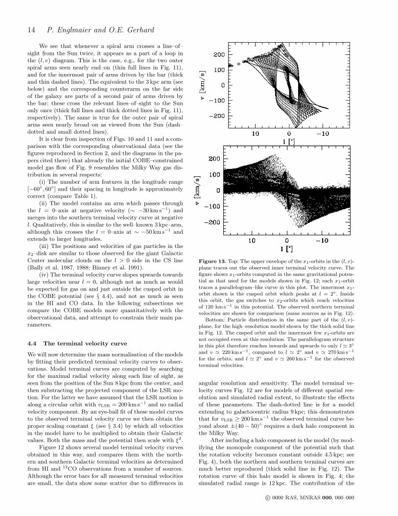
Figure 13. Top: The upper envelope of the x1-orbits in the (l, v)-plane traces out the observed inner terminal velocity curve. Thefigure shows x1-orbits computed in the same gravitational poten-tial as that used for the models shown in Fig. 12; each x1-orbit

traces a parallelogram–like curve in this plot. The innermost x1-orbit shown is the cusped orbit which peaks at l = 2. Insidethis orbit, the gas switches to x2-orbits which reach velocitiesof 120 km s−1 in this potential. The observed northern terminalvelocities are shown for comparison (same sources as in Fig. 12).

Bottom: Particle distribution in the same part of the (l, v)-plane, for the high–resolution model shown by the thick solid linein Fig. 12. The cusped orbit and the innermost few x1-orbits arenot occupied even at this resolution. The parallelogram structurein this plot therefore reaches inwards and upwards to only l ≃ 3

and v ≃ 220 km s−1, compared to l ≃ 2 and v ≃ 270 km s−1

for the orbits, and l ≃ 2 and v ≃ 260 km s−1 for the observedterminal velocities.

angular resolution and sensitivity. The model terminal ve-locity curves Fig. 12 are for models of different spatial res-olution and simulated radial extent, to illustrate the effectsof these parameters. The dash-dotted line is for a modelextending to galactocentric radius 9 kpc; this demonstratesthat for vLSR ≥ 200 kms−1 the observed terminal curve be-yond about ±(40 − 50) requires a dark halo component inthe Milky Way.

After including a halo component in the model (by mod-ifying the monopole component of the potential such thatthe rotation velocity becomes constant outside 4.5 kpc; seeFig. 4), both the northern and southern terminal curves aremuch better reproduced (thick solid line in Fig. 12). Therotation curve of this halo model is shown in Fig. 4; thesimulated radial range is 12 kpc. The contribution of the

c© 0000 RAS, MNRAS 000, 000–000


Figure 12. Northern and southern Galactic terminal velocity curves compared with model predictions. Observational data from sourcesas follows. Filled squares (l = 0 − 10): HI data from Fig. 1 of Burton & Liszt (1993). Empty squares (l = 0 − 20): unpublished140ft single dish HI data, kindly provided by Dr. B. Burton. Open circles: HI terminal velocities from Fich et al. (1989), based on datafrom Westerhout (1957). Diamonds, with tiny error bars: northern 12CO terminal velocities from Clemens (1985). Without error bars:southern 12CO data from Alvarez et al. (1990). The data are relative to the LSR, mostly as corrected by the respective authors. TheClemens (1985) data have been corrected for internal dispersion, and the velocities in Burton & Liszt (1993) are relative to the Sun andhave been corrected for LSR motion.

The model terminal velocity curves are from: a typical low resolution model with no halo and declining rotation curve (dash–dotted);the same model at higher resolution but with less radial extent (dotted); a low resolution model with flat rotation curve (thin solid); andour best model with high resolution (see text) and flat rotation curve (thick solid line). All models assume a bar angle ϕbar = 20 andhave corotation at Rc ≃ 3.4 kpc.

c© 0000 RAS, MNRAS 000, 000–000


dark halo inside the solar radius is fairly small (∼ 23% inthe radial force at 8 kpc), somewhat less even than in Kent’s(1992) maximum disk model.

In this model, there remain two main regions of dis-crepancy with the observed terminal velocity curve. First,the model terminal velocities are too low at and just out-side the peak at l ≃ 2. This is strongly influenced by andprobably due to resolution effects, as discussed below. Sec-ond, there is a larger mismatch around −20. This is likelycaused by our mass model not being correct in the vicinityof the NIR lumps ∼ 3 kpc down the minor axis of the bar.Lines–of–sight at around −20 cross one of these lumps aswell as the end of the 3 kpc arm and the head of one of thespiral arms outside corotation (see Fig. 11). The eight-foldsymmetric deprojection of BGS is therefore likely to give in-correct results in this region. Smaller systematic deviationsin the terminal velocities are visible around l = 30−50 andl = −(50 − 70), although there, and everywhere else, thedifferences between model and observations are now of theorder of the scatter between the various observational dataand of the order expected from perturbations in the disk.Given the uncertainties the overall agreement is surprisinglygood. This suggests that the basic underlying assumption,that in the inner Galaxy the NIR light traces the mass, ismostly correct.

Fitting the terminal velocity curve to both sides we ob-tain a scaling constant of ξ = 1.12. This is slightly largerthan the value obtained in our first attempts to fit the mod-els to the observations (ξ = 1.075, Bissantz et al. 1997), inwhich we only considered the northern rotation curve andignored the data beyond l = 48. It is worthwhile pointingout that the derived value of ξ is only weakly dependent onthe assumed LSR tangential velocity: In order of magnitude,a 10% change in the LSR velocity leads to a 1% differencein ξ. With an improved dust model and deprojection of theouter disk we could therefore attempt to determine V0 fromthese models.

As is clearly visible in Fig. 12, the peak in the observedterminal curve at 2 is not well reproduced by our lower–resolution models. However, Fig. 13 shows that it is nicelyapproximated by the envelope of the x1–orbit family whenall orbital velocities are scaled by the same value of ξ. Atearly times in the model evolution, when the gas flow isnot yet stationary, the peak is also reproduced in the hy-drodynamic gas model, but thereafter the region aroundthe cusped orbit is depopulated (see also Jenkins & Bin-ney 1994). We attribute this to the artifical viscosity in theSPH method, which smears out the velocity gradient overtwo smoothing lengths, and to the method used for settingup the gas simulation.

We can estimate the magnitude of the effect as follows.Near the cusped orbit, which sets the maximum velocityalong the terminal velocity curve, the particle smoothinglength h in the low resolution model is large, about ∼ 100 pc,because the gas density in this region is small. The full x1–orbit velocity on the terminal curve can only be reachedabout two smoothing lengths away from the cusped orbit,where it is no longer affected by the more slowly movinggas on x2–orbits further in. The longitudinal angle corre-sponding to about 2h at the distance of the galactic centreis about 1.4. Thus, the peak in the gas dynamical terminal

curve should be found at l > 3.4 when the orbits peak at2, showing how sensitive the peak location is to resolution.

To test this explanation, we have run a bi-symmetricmodel with 100, 000 particles, resulting in about 2.2 times asmuch spatial resolution as in the low–resolution models. Juston the basis of this higher resolution, the terminal velocitypeak then moves from about 5 to 4 (at t = 0.3 Gyr). Wethen further increased the resolution by the following proce-dure. The gas inside the outermost x1 orbit shown in Fig. 6was removed, and set up again on nested closed x1 and x2

orbits, while keeping particles outside this region unchanged.Evolving this modified gas distribution for a further 0.3 Gyr,we obtained our final high resolution model. This is shownby the thick solid line in Fig. 12, which peaks at about 3

and vt = 235 kms−1. Compared to the original 20000 par-ticle model (thin solid line in Fig. 12) the mismatch at thepeak has been reduced by about a factor of two in scale andby two thirds in the peak velocity.

Although this analysis was inspired by a technical prob-lem, there is an observable implication of it as well. Sincewe may interpret the hydrodynamical model in terms of gasclouds having a mean free path length of order the smooth-ing length, we may restate the result in the following way:a loss of resolution occurs when the cloud mean free pathis significant compared to the gradient in the true velocityfield. Applied to the inner Galaxy, our result then indicatesthat the clouds near the cusped orbit peak in the termi-nal velocity curve must have short mean free paths, i.e., bedescribed well in a fluid approximation.

Apart from resolution effects, the precise position of thepeak in the terminal velocity curve also depends criticallyon the location of the ILR and hence on the mass model inthe central few 100 pc. In this region, the deprojected COBEmodel suffers from a lack of resolution and our added nuclearcomponent has uncertainties as well. We therefore believethat with improved data and further work the remainingdiscrepancies in this region will be fixed.

4.5 Pattern Speed and Orientation of theGalactic Bar

There are two observations which constrain the value of thepattern speed rather tightly. First, there is the 3-kpc-arm,a feature which exhibits non-circular motions of at least50 kms−1. In our models, we find that only the arms in-side the bar’s corotation radius are associated with strongnon-circular motions, so such an arm has to be driven bythe bar. From observations and models of barred galaxieswe also know that strong spiral arms associated with bothends of a bar are common. Therefore we conclude that the3-kpc-arm must lie inside the bar’s corotation radius.

Second, a lower limit to the corotation radius is givenby the inner edge of the molecular ring. If the molecularring were indeed a ring such as induced by a resonance, itwould be located near the outer Lindblad resonance (e.g.,Schwarz 1981). On the other hand, if it is actually made ofseveral spiral arms (Dame 1993, Vallee 1995, this paper),then the small observed non-circular velocities along thesespiral arms also show that these arms must be outside thebar’s corotation radius. Solomon et al. (1985) find from thedistribution of hot, presumely shocked cloud cores, that theinner edge of the molecular ring is at R = 4kpc. The total

c© 0000 RAS, MNRAS 000, 000–000


Figure 14. Longitude–velocity (l, v) diagrams for the gas flows in COBE bar potentials with different pattern speeds and bar orientationangles. The column of (l, v) diagrams on the left shows the influence of the pattern speed on the gas flow in the standard ϕbar = 20

COBE bar potential. These frames show models with corotation radii Rc = 3.1 kpc (top) Rc = 3.4 kpc (middle) to Rc = 4.0kpc (bottom).The right column shows gas flows in COBE bars deprojected for different bar orientation angles, ϕbar = 15 (top), ϕbar = 25 (middle),ϕbar = 30 (bottom), all for corotation at Rc = 3.4 kpc.

surface density of neutral gas also drops dramatically insideof 4 kpc (Dame 1993). From the IRT 2.4 µm photometry ofthe galactic disk Kent et al. (1991) concluded that thereis a ring, or spiral arm, at about R = 3.7 kpc. Thereforewe conclude that the bar’s corotation radius is inside R =4 kpc.

An independent argument for corotation falling some-where between 3 kpc and 4 kpc comes from the fact that thedeprojected COBE bar appears to end somewhere between3 kpc and 3.5 kpc (BGS). From both N–body simulationsand direct and indirect observational evidence the corota-

tion radius is usually found at between 1.0 and 1.2 timesthe bar length (Sellwood & Wilkinson 1993; Merrifield &Kuijken 1995; Athanassoula 1992b). In our models, a cora-tion radius between 3 kpc and 4 kpc corresponds to a patternspeed of ∼ 50 − 60 kms−1kpc−1.

We have run gas dynamical simulations with corota-tion at 4.0, 3.4, and 3.1 kpc, to determine from observationswhich of these values is most nearly appropriate. For thecomparison with observations it is important to notice thatseveral other parameters enter here, most importantly, theorientation angle of the bar, the uncertain contribution of

c© 0000 RAS, MNRAS 000, 000–000


the dark halo to the outer rotation curve and hence terminalvelocities, and the LSR velocity.

We first fix the bar orientation angle at ϕbar = 20,but will vary this parameter later. The chosen value of ϕbar

is in the range allowed by the NIR photometry (BGS), it isfavoured by the clump giant star distribution as analyzed byStanek et al. (1997) and by the gas kinematical analysis ofthe molecular parallelogram by Binney et al. (1991), and itmeets the preference for an end–on bar in the interpretationof the microlensing experiments.

In the last section we found that the Galactic terminalvelocity curve for |l| ≤ 45 is well–reproduced by the gasflow in the maximum NIR disk model with constant mass–to–light ratio. Moreover, even this maximum disk model failsby a factor of ∼> 2 in explaining the high microlensing opti-cal depth towards the bulge (Bissantz et al. 1997), makingit very difficult to further reduce the mass in the interven-ing disk and bulge. We can therefore confidently assume amaximum disk model in the following and, to separate thedetermination of the bar and halo parameters, we restrictthe comparison with observations to longitudes |l| ≤ 45.

Finally, we set the LSR rotation velocity to V0 =200 kms−1, in the middle of the observed range (§2.7). A10% difference in this parameter is not very important forthe comparison with the inner Galaxy gas velocities.

Thus we begin by considering a sequence of modelswith varying corotation radius Rc and the other parametersfixed as just described. For three models with Rc = 4.0 kpc,3.4 kpc, and 3.1 kpc we have plotted (l,v) diagrams and havedetermined the scaling constant ξ for each simulation by fit-ting to both terminal curves. The final scaled (l, v) diagramsare shown in the left column of Fig. 14. For the scaling con-stant we obtain ξ = 1.13, 1.12, and 1.09 for the 4.0, 3.4,and 3.1 kpc models. The correctly scaled pattern speeds arethen 59, 57, and 61 kms−1kpc−1. This means that by chang-ing the corotation radius, we effectively change the mass ofthe model galaxy, while keeping the pattern speed almostconstant at about 60 kms−1kpc−1.

At small absolute longitudes, |l| ≤ 10, these low–resolution models do not have enough particles to resolvethe true gas flow, and furthermore there are no publishedterminal velocities in this region on the southern side. Thusfor now we ignore data near the peak of the terminal velocitycurve. This leaves a range of ±l = 10− 45 within which wecompare these no–halo model gas flows with the northernand southern terminal velocity curves and with the variousspiral arm features shown in Figs. 1–2.

On the northern side (l > 0), we try to match the modelto the pronounced spiral arm at about +30, which is bestvisible in the warm CO clouds (Solomon et al. 1985) and inthe distribution of HII-regions. Moreover, the (l,v)-diagramsof CO and HII-regions shows that the +30 arm is double(Fig. 2). In the model shown schematically in Fig. 11, thereare actually three arms near l ≃ 30, two of which overlap,while the third, the northern 3-kpc-arm (thick dotted line),runs almost parallel to the first two. There is also a wiggle inthe terminal curve at about +10, which is probably causedby a spiral arm similar to the northern, secondary innerspiral arm in the model (thin dashed line in Fig. 11). Thesouthern terminal curve is more distorted by spiral armsthan the northern curve. A pronounced feature is the −30

arm in the molecular ring, as well as the well–known 3-kpc-

arm which continues on from a non–circular velocity ridgebeginning at l ≃ 10 and v = 0.

Fig. 14 (left column) shows that the gas flows in all threecases are similar; nonetheless small differences in the spiralarm locations help to show that the 3.4 kpc case is closestto the real Galaxy. The 30 spiral arm tangent is best re-produced in the 3.4 kpc-model (middle panel in left columnof Fig. 14). In the top panel, it is not double as observed,and in the bottom panel the tangent moves out to ∼ 40.The 50 spiral arm tangent is reasonably well reproduced inthe top two panels, but is absent or very weak in the bot-tom panel, but this arm may not be a reliable indicator inthe absence of a halo. In the south, we observe that largecorotation radii move the arm at −30 outwards. The −30

spiral arm tangent is in about the correct location in the toptwo panels, but too far out in the bottom panel. The mis-match of the terminal curve at about −20 becomes largerwith decreasing corotation radius as well. On the other hand,the −50 spiral arm tangent is not present for the largestpattern speed (top panel), while it is adequately present inthe lower two panels. The 3-kpc-arm equivalent is presentin all three models, but its detailed locus in the (l, v) dia-gram is not correct in any of the models: it has either toolow non–circular velocities at l = 0 (particularly in the bot-tom panel), or it does not extend to large enough negativelongitudes (particularly in the top panel). For corotation at3.4 kpc, the 3-kpc-arm ends in the model exactly at 3 kpc, asseen from the assumed solar position. There are particles inthe low intensity forbidden velocity region bounded by theline from (l, v) = (10, 0) − (0,−50) in all three models, butthe resolution does not suffice to prefer one model over theother. Finally, an equivalent to the 155 kms−1 arm at smallnegative l is present only for the lowest pattern speed.

From an unweighted average of these comparisons tovarious observational landmarks we conclude that the coro-tation radius of the Galactic bar is most likely at about3.4 kpc. However, since none of the above models is exactlyright yet, this value could well change by 10% when othereffects are taken into account, such as bar orientation (dis-cussed next), dark halo (§4.6), or self–gravitating spiral arms(§4.7).

With the corotation radius fixed at 3.4 kpc, we can at-tempt to find an optimal orientation angle for the bar. Forthis purpose, a series of deprojected bar models have beenmade as in BGS, for bar orientation angles ϕbar = 10, 15, 20,25, and 30. Smaller or larger angles are not consistent withthe asymmetry pattern of the observed NIR distribution orresult in unphysical bar shapes, see BGS and Bissantz et al.(1997). With the bar orientation the shape and radial extentof the deprojected bar change.

Gas flow simulations with Rc = 3.4 kpc were made foreach of these cases, and (l, v) diagrams for ϕbar = 15, 25, and30 are shown in the right column of Fig. 14. We observedthat the resulting changes in the model terminal velocitycurves are caused in about equal parts by the change in theviewing direction relative to the bar, and by the intrinsicdifferences between the deprojected mass distributions. Themodels’ scaling factors ξ are again determined separatelyfor each model by eyeball fitting the observed northern andsouthern terminal curves. The variation in ξ is very small,however: we obtain ξ = 1.1, 1.11, 1.12, 1.11, and 1.12 fororientation angles from 10 to 30.

c© 0000 RAS, MNRAS 000, 000–000


We find only a weak preference for the 20 model.The −30 arm is more consistent with the 10 and 15

case, whereas these models show too large terminal veloci-ties around +40. The +30 arms seem to be in favour of15 − 25, whereas the 3-kpc-arm, although always too slowat l = 0, seems to fit slightly better with 20. We concludethat the orientation is about 20 with a large uncertainty.

4.6 Spiral arm tangents

In the previous §4.5 we have already used the observed spiralarm tangents at l = ±30 to constrain the pattern speedand orientation angle of the bar. Here we reconsider thelocation of the spiral arms in the models that compared bestwith the Galaxy in §4.5 (i.e., those with Rc = 3.4 kpc andϕbar = 20), but with (i) a possible dark halo included, (ii)emphasis also on the nearby terminal curve and the spiralarms with tangents at l = ±50, and (iii) higher resolution.

For comparing the model spiral arms with observationswe again use the tracers in Fig. 2 (HII regions and molecu-lar clouds) and the characteristic features in (l, v) diagramslike Fig. 1. Unfortunately, because the structures in the ob-served (l, v) diagrams are much less sharp than in the model(l, v) diagrams, it is very difficult to measure reliably anyfeatures beyond those already discussed, i.e., the spiral armtangent point positions, the 3–kpc arm and the molecularring. Already the run of the arms out of the molecular ringto their tangent points cannot be identified unambiguouslyfrom Fig. 1.

Spiral arm tangent directions in the models are easilydetermined. When the arm is broadened in the tangentialdirection, we place the tangent at the outer edge, where thevelocity jump is. In this way we can achieve a fair accuracyof a few degrees. Only one tangential direction, the Scutumarm at l = 30, cannot easily be determined in this way, be-cause its tangent goes through the corotation region throughwhich no arm continues inwards in the model. Nevertheless,we can measure an approximate value for this tangent aswell. Table 1 gives a comparison of model and observed spi-ral arm tangent directions, and the various data that havebeen used for the observed directions.

The bar–driven spiral arms in the models change theirrelative strength, opening angle, and hence location, depend-ing on pattern speed, bar orientation, halo mass contribu-tion and other parameters. In §4.5 we have discussed theconstraints on the the pattern speed and bar orientation an-gle. Fig. 15 shows that adding a dark halo mass contributionso as to make the outer rotation curve flat (at 208 km s−1

after scaling) has the following two effects: (i) the outer pairof spiral arms at l = ±50 now form a more regular pat-tern with the inner pair at l = ±30, and all four arms nowhave a similar density contrast with respect to the interarmgas; (ii) all four tangent directions now fit the observationsreasonably well; see also Table 1. Fig. 15 also shows the po-sitions of large HII-regions and molecular clouds superposedon the gas arms. Note that their distances were determinedfrom a circular orbit model and so may be slightly in error.Nonetheless it is reassuring that they fall approximately onthe model gas arms, consistent with the model’s match tothe spiral arm tangents.

4.7 Gravitating spiral arms

In this section we estimate the effect, if any, of the gravi-tational potential of the stellar spiral arms that are likelyassociated with the spiral arms seen in the gas. Rememberthat in our model, the spiral arms outside the bar’s corota-tion radius are driven by the clumps of NIR light and mass∼ 3 kpc down the minor axis, which rotate with the bar (see§4.1). We interpret these clumps as the signature of real spi-ral arms in the deprojected NIR light. In the gas model twoof the spiral arm heads are about at the correct positionswhere these clumps are observed; this supports the view thatthe gravitational potential of the clumps is a first estimateof the true spiral arm potential.

However, the models discussed sofar did not take intoaccount the gravitational perturbations outside the clumpregions that could be associated with the spiral arms. Inparticular, we are interested in knowing whether the mor-phology of the spiral arms would be changed when thesearms carry a reasonable fraction of the mass throughout thedisk. To test this, we have experimented with the followingscheme that makes use of the particular strengths of the SPHmethod: First, we assign a fraction of the mass of the NIRdisk to the spiral arms. Most of this mass will be associatedwith the spiral arm perturbation in the stellar density. Thenwe assign this part of the mass to the gas particles, assumingthat a large fraction of the gas will later be concentrated inthe arms and that the shock fronts seen in the gas will tracethe stellar spiral arm crests. Finally, to mimic the fact thatthe stellar spiral arms are much broader in azimuth thanthe shocks seen in the gas, we set the gravitational soften-ing radius of the gas particles to a value appropriate for thestellar arm widths and different from the smoothing lengthused in the calculation of the hydrodynamic forces.

According to Rix & Zaritsky (1995), the spiral armscover about one third of the surface area in galaxies mor-phologically similar to the MW. The arm–interarm contrastis somewhat less than average for these galaxies, so that weestimate that about 20% of the total NIR luminosity is in thespiral arms (superimposed on the axisymmetric backgrounddisk which thus contributes about 80%).

The azimuthally averaged surface density associatedwith the spiral arms should thus also be ∼ 20% of the meanbackground stellar surface density. In the solar neighbor-hood, the stellar surface density of our normalized models is35ξ2M⊙ pc−2. Thus we first take an ‘arm’ potential corre-sponding to a mean surface density of 7M⊙ pc−2 at the solarradius, and a factor exp[−(r − 8 kpc)/2.5 kpc] more furtherin. Here we have used the radial scale-length of the NIR diskfrom §3. This spiral arm mass is given to the gas particles,and in order to compensate for the extra mass, we substractthe same amount as a constant fraction from the COBE NIRmass model.

Because the stellar spiral arms are less sharp thangaseaus arms, we estimate their gravitational force bysmoothing the gravitational forces of the gas particles oversome length scale ε. Each particle contributes a smoothedpotential

φi(r) = − Gm∗i√

(r − ri)2 + ε2(5)

to the gravitational field of the ‘arms’. Here, m∗i denotes

c© 0000 RAS, MNRAS 000, 000–000


Figure 15. Spiral arm tangents in two models with ϕbar = 20 compared to observations. Left: standard model without dark halo;right: including dark halo. Both models are computed with 100,000 particles and the gas disk is truncated at 10 kpc.The observed directions of spiral arm tangents are shown by the straight lines, starting at the position of the Sun at x = −7.5 kpc,y = −2.7 kpc in this plot. See Table 1 which also lists the spiral arm tangents for the models. For illustration, stars denote positions ofmajor HII-Regions from Georgelin & Georgelin (1976) and Georgelin et al. (1996), and circles the positions of large molecular clouds fromDame et al. (1986) and Grabelsky et al. (1988). The distances of these tracers have been rescaled to R0 = 8kpc but are not correctedfor non-circular motions. Such a correction would tend to move HII-Regions into the model spiral arms, because of velocity crowding.

the stellar mass associated with particle i; m∗i is obtainedby dividing the total mass in the stellar spiral arms by theeffective number of gas particles. The parameter ε must de-pend on the average distance between two arms in the model(about 3 kpc in the region of interest). We thus mimic thebroader spiral arm potential by smoothing the gas arm po-tential over about ε ∼ 1 kpc.

Notice that the hydrodynamical forces do not dependon the actual value of the surface mass density, but only onthe particle density gradient. We can therefore save somememory space by taking the SPH particle mass mi equal tothe stellar m∗i.

The initial gas disk is set up in a similar way as for themodels discussed above, but for consistency the surface den-sity is that of an exponential disk with the same radial scalelength as the stellar disk. The resulting additional radialpressure gradient is far to weak to change the dynamics.

In our first attempt at such a model we found that the

mass in the gas particles accumulating on the x2-disk due toinflow was so large that the rotation curve in this region waschanged significantly. Moreover, the dust lane shock frontsacquired significant mass. This is unrealistic since no strongstellar arms form at the edge of the bar, and it has the effectof changing the gas flow near the cusped orbit. To avoid botheffects we have set the gas particle masses to zero insidethe bar region, which was approximated by an ellipse withmajor axis 3 kpc and minor axis 1.8 kpc. Correspondingly,the COBE mass model was then not changed in this region.

The gravitating arm model with the specified parame-ters that finally results is shown in the left panels of Fig. 16.First, we notice that the distribution of gas has not changedmuch compared to Fig. 15. Especially the locations of thearms are unchanged. The inner arms now contain more par-ticles, because of the initial exponential surface density pro-file. However, the line–of–sight velocities have been modifiedsomewhat. For example, the 3-kpc-arm has now about the

c© 0000 RAS, MNRAS 000, 000–000


Figure 16. Model with additional spiral arm potential. Left: case with realistic parameters; right: twice as high surface density, and halfas large gravitational smoothing lengths.

right velocity: ≃ −41 kms−1 at l = 0. At around l = 20

the terminal velocities are now larger than the observed ve-locities. On the southern side, at l ∼ −20, the velocitiesare also higher, removing part of the previous discrepancybetween model and observation. The larger velocities in thisregion are probably due to the mass in the 3-kpc-arm andthe second arm at ∼ 2 kpc and their symmetric counterarms.

We have also run a model with about twice as muchmass in the ‘arm’ potential and half the smoothing length,ε = 0.5 kpc (right panels of Fig. 16). Both parameter in-crease the gravitational response to the arms and are ex-treme values for the Milky Way. In this case, the distribu-tion of the gas has changed more dramatically, especially inthe region close the the bar. The inner arms seem to forman ellipse around the bar; however, the number of arms hasstill not changed. The 3-kpc-arm in this model is faster thanthe observed 3-kpc-arm and expands with 60 kms−1 towardsthe observer at l = 0, but it no longer extends out to 3 kpc.The model terminal curve now gives only a poor fit to theobservations. One interesting property of this model is thatit contains much more gas with forbidden velocities than allour other models.

From both models it is clear that the gravitational po-

tential of the spiral arms is important for the comparisonwith Galactic (l, v) diagrams at a level of ∼ 15 kms−1. Es-pecially the 3-kpc-arm and details in the terminal velocitycurve depend on this parameter. Besides that, however, themorphology and spiral arm tangents are not effected much.It is encouraging that the inclusion of spiral arm gravity ap-pears to improve the fit to some aspects of the data, eventhough the models discussed in this section certainly donot contain the entire story. For example, we have not sub-tracted a fraction of the mass in the minor axis NIR clumpswhich should now be taken care of by the spiral arms. Ona more fundamental level, it is quite possible that the spi-ral arms between the bar and the solar circle rotate with asomewhat different pattern speed from that of the bar (seeSellwood & Wilkinson 1993 for a review of this subject, andAmaral & Lepine 1997 for a separate model of the Galac-tic spiral arms with a slow pattern speed). If this were thecase, we would have to observe the resulting time–dependentpattern of bar and spiral arms at a moment when both theapparent NIR distribution of light and the induced kine-matical perturbations resemble those observed in the MilkyWay. This may not be as difficult as it appears because ofthe Galaxy’s relatively tightly wound four–armed spiral pat-

c© 0000 RAS, MNRAS 000, 000–000


tern. However, simulating this would introduce an entirelynew degree of freedom and will not be attempted here.

5 CONCLUSIONS

We have presented a new set of hydrodynamical modelsfor the gas flow in the Galactic disk inside the solar circle.These gas flows are evolved in the gravitational potentialsobtained by deprojecting the NIR luminosity distribution ofthe Galactic bar and disk from COBE/DIRBE under theassumption of eight–fold symmetry (as in Binney, Gerhard& Spergel 1997), assuming constant mass–to–light ratio forthe NIR luminous material, and adding a nucleus and (insome cases) a dark halo component. These models allow usto understand many features of Galactic HI and CO obser-vations.

To follow the gas dynamics we have used the SmoothParticle Hydrodynamics (SPH) code described in Englmaier& Gerhard (1997). With the SPH method we can resolvethe spiral arm shocks well, and use them in some modelsas tracers for the gravitational potential of the stellar spi-ral arms. The hydrodynamical models quickly settle to anapproximate quasi–equilibrium flow pattern whose overallmorphology is not sensitive to the precise value of the bar’spattern speed, to the orientation of the bar with respect tothe observer, and to whether or not the spiral arms carrymass.

We have compared our gas models with Galactic HI,CO, HII, and other data. We find that these models providea coherent explanation of many aspects of the data, suchas: (i) the four–armed spiral structure of the Milky Waybetween corotation and the solar radius, (ii) the nature ofthe 3–kpc–arm, (iii) the terminal velocity curve, (iv) thenon–circular velocities near the cusped orbit at the ILR,and (v) the disk of gas on the inner x2–orbits. Thus NIRphotometry and gas kinematic observations conform to asingle picture, and the Galactic bar is an essential part ofthis.

In this picture, the bar (bulge) rotates with a patternspeed such that corotation is at Rc ≃ 3.5 ± 0.5 kpc. The3-kpc arm is one of the arms emanating from the ends ofthe bar, extending into the corotation region. Outside coro-tation, a four–armed spiral arm pattern gives rise to themolecular ring and the arms extending to the solar circleand beyond. In the model, this pattern is generated by therotating luminosity/mass concentrations on the bar’s minoraxis found by BGS. These can therefore not just be dueto light from young supergiant stars, but must be massive;most likely they are symmetrized approximations to the stel-lar spiral arms themselves. A spiral pattern similar to thatfound here has been observed by Fux (1998) in those of hisN–body – SPH barred galaxy models which compare best tothe Galactic (l, v) diagrams. These models start from a setof specified initial conditions rather than from observations.The fact that both approaches lead to similar overall resultsis encouraging.

We find that the Galactic terminal curve out to longi-tudes l ≃ 45 is consistent with a maximal, constant mass–to–NIR light disk and bar model. The inferred mass in thedisk cannot easily be reduced because (i) this model still un-derpredicts the microlensing optical depth towards the bulge

(Bissantz et al. 1997) and (ii) it predicts about the correctsurface mass density for the old stellar disk near the Sun.Thus the Galactic dark halo will be an important contribu-tion to the mass of the Milky Way only outside of at leastR = 5kpc, depending on the LSR rotation velocity.

The models are similar and in reasonable overall agree-ment with the Milky Way observations for a range of val-ues of the bar’s orientation angle. Probably best is ϕbar =20 − 25 but the uncertainties are are such that 15 or 30

cannot be excluded. The detailed match to various key ob-servational quantities does depend on ϕbar and the precisevalue of Rc, but at a level comparable to the influence ofvarious other parameters including the LSR rotation veloc-ity, the asymptotic halo circular speed, and the influence ofthe stellar spiral arm gravity.

Some features of the HI and molecular emission datacan be reproduced quantitatively, such as the Galactic spi-ral arm tangent positions, much of the terminal velocitycurve, or the position of the nuclear x2–disk. On the otherhand, a detailed quantitative fit to all features in the ob-served (l, v) diagrams is not yet possible. The 3-kpc armin the model has the correct angular extent but somewhattoo small non-circular velocities. Its arm tangent positioncoincidences with the place where the model terminal curvediffers most from the observations. In this region the diskmass model may not be very accurate. The position and ve-locity of the molecular parallelogram are fitted well by closedorbits in the NIR potential, whereas the hydrodynamic gasflow underestimates the velocity and overestimates its radialscale. Probably both hydrodynamic resolution and uncer-tainties in the potential near ∼ 200 pc (where the NIR datahave insufficient resolution) are responsible for this. Also,this suggests that the clouds near the peak of the terminalvelocity curve have a small mean free path.

Much work remains to be done. Because the deprojecteddisk model accounts only insufficiently for the Galactic spiralarms, some aspects of the gravitational potentials used arelikely to be wrong. With a model for the spiral arms inhand, both the correction of the NIR data for dust and thesubsequent deprojection of these data could be improved.Further observational work on spiral arm tracers such asHII regions and molecular clouds would be highly valuablefor clarifying the run of the weaker Galactic spiral armsand those on the other side of the bar, and thus for betterconstraining the gas-dynamical models. Distance estimatesto these tracers could be improved by making use of thevelocity fields in these models.

On a more fundamental level, several assumptions madein the models may be or are likely to be invalid at somelevel, and require further study: (i) that the gravitationalpotential and gas flow structures are quasi-stationary andpoint–symmetric with respect to the Galactic Centre; (ii)that the NIR light is a fair tracer of the stellar mass, i.e.,that young supergiant stars do not contribute significantlyto the NIR light (but see Rhoads 1998); (iii) that the gasdisk can be treated as planar; (iv) and that the bar andspiral arms rotate with the same pattern speed.

c© 0000 RAS, MNRAS 000, 000–000


ACKNOWLEDGMENTS

We are grateful to M. Steinmetz for many discussions onSPH and for making his original code available. We thankB. Burton, L. Bronfman, T. Dame and H. Liszt for send-ing data, some in advance of publication. We also thankT. Dame for producing Figure 1 and M. Samland for helpwith plot software. We acknowledge helpful discussions withJ. Binney, T. Dame, R. Fux and M. Samland. This workwas supported by the Swiss NSF grants 21-40’464.94 and20-43’218.95, and the NASA grants WKU-522762-98-6 andNAG5-3841.

REFERENCES

Alcock C., et al. , 1997, ApJ, 479, 119Amaral L.H., Lepine J.R.D., 1997, MNRAS 286, 885Alvarez H., May J., Bronfman L., 1990, ApJ, 348, 495

Athanassoula E., 1992a, MNRAS, 259, 328Athanassoula E., 1992b, MNRAS, 259, 345Bally J., Stark A.A., Wilson R.W., Henkel C., 1987, ApJS, 65, 13

Bally J., Stark A.A., Wilson R.W., Henkel C., 1988, ApJ, 324,223

Becklin E.E., Neugebauer G., 1968, ApJ, 151, 145Beuermann K., Kanbach G., Berkhuijsen E.M, 1985, A&A, 153,

17

Binney J.J., Gerhard O.E., 1996, MNRAS, 279, 1005Binney J.J., Gerhard O.E., Spergel D., 1997, MNRAS, 288, 365Binney J.J., Gerhard O.E., Stark A.A., Bally J., Uchida K.I.,

1991 MNRAS, 252, 210Bissantz N., Englmaier P., Binney J.J., Gerhard O.E., 1997, MN-

RAS, 289, 651Blitz L., Spergel D.N., 1991, ApJ, 379, 631

Bloemen J.B.G.M., Deul E.R., Thaddeus P., 1990, A&A, 233, 437Bronfman L., 1992, in: The Center, Bulge, and Disk of the Milky

Way, Blitz L., ed, Kluwer, Dordrecht, 131Bronfman L., Nyman L., Thaddeus P., 1989, Lecture Notes in

Physics, 331, 140

Burton W.B., 1985, A&AS, 62, 365Burton W.B., 1992, in: The Galactic Interstellar Medium, eds.

Pfenniger D., Bartholdi P., Saas-Fee Advanced Course 21,Springer–Verlag.

Burton W.B., Liszt H.S., 1978, ApJ 225, 815

Burton W.B., Liszt H.S., 1992, A&AS, 95, 9Burton W.B., Liszt H.S., 1993, A&A, 274, 765Burton W.B., Shane W.W., 1970, in: The Spiral Structure of

Our Galaxy, IAU Symp. 38, eds. W. Becker, G. Contopoulos,Reidel, Dordrecht, 397

Caswell J.L., Haynes R.F., 1987, A&A, 171, 261Catchpole R.M., Whitelock P.A., Glass I.S., 1990, MNRAS, 247,

479Chen W., Gehrels N., Diehl R., Hartmann D., 1996, A&AS, 120,

315

Clemens D.P., 1985, ApJ, 295, 422Cohen R.J., Cong H., Dame T.M., Thaddeus P., 1980, ApJ, 239,

L53Cohen R.J., Few R.W., 1976, MNRAS, 176, 495

Contopoulos G., Papayannopoulos T., 1980, A&A, 92, 33Cowie L.L., 1980, ApJ, 236, 868Dame T.M., 1993, in: Back to the Galaxy, eds. Holt S.S., Verter

F., AIP 278, American Institute of Physics, 267

Dame T.M., Elmegreen B.G., Cohen R.S., Thaddeus P., 1986,ApJ, 305, 892

Dame T.M., et al. , 1987, ApJ, 322, 706

Dame T.M., et al. , 1998, in prep.Downes D., Wilson T.L., Bieging J., Wink J., A&AS, 40, 379

Dwek E., et al. , 1995, ApJ, 445, 716

Englmaier P., Gerhard O.E., 1997, MNRAS, 287, 57

Freudenreich H.T., 1998, ApJ, 492, 495Fich M., Blitz L., Stark A.A., 1989, ApJ, 342, 272

Fux R., 1998, in preparationGeorgelin Y.M., Georgelin Y.P., 1976, A&A, 49, 57

Georgelin Y.M., et al. , 1996, A&AS, 120, 41Gerhard O.E., 1996, in: Unsolved Problems of the Milky Way,

IAU Symp. 169, eds. L. Blitz, P. Teuben, Kluwer, Dordrecht,79

Gerhard O.E., Vietri M., 1986, MNRAS, 223, 377Grabelsky D.A., Cohen R.S., Bronfman L., Thaddeus P., 1987,

ApJ, 315, 122

Grabelsky D.A., Cohen R.S., Bronfman L., Thaddeus P., 1988,ApJ, 331, 181

Hartmann D.A.P., Burton W.B., 1997, Atlas of galactic neutralhydrogen, Cambridge, New York, Cambridge University Press

Hayakawa S. et al. , 1981, A&A, 100, 116Heiligman G.M., 1987, ApJ, 314, 747

Henderson A.P., 1977, A&A, 58, 189

Jenkins A., Binney J.J., 1994, MNRAS, 270, 703Kent S.M., 1992, ApJ, 387, 181

Kerr F.J., Bowers P.F., Kerr M., Jackson P.D., 1986, A&AS, 66,373

Kent S.M., Dame T.M., Fazio G., 1991, ApJ, 378, 131

Kuijken K., 1996, in: Barred Galaxies, IAU Coll. 157, eds.R. Buta, D.A. Crocker, B. G. Elmegreen, ASP, San Francisco,504.

Kuijken K., Tremaine S., 1994, ApJ, 421, 178

Lindqvist M., Habing H.J., Winnberg, A., 1992, A&A 259, 118Liszt H.S., Burton W.B., 1980, ApJ, 236, 779

Lockman F.J., 1979, ApJ, 232, 761Lockman F.J., 1989, ApJS, 71, 469

Merrifield M.R., Kuijken K., 1995, MNRAS 274, 933Mihalas D., Binney J.J., 1981, Galactic Astronomy, 2nd ed., San

Francisco: Freeman.

Monaghan J.J., Gingold R.A., 1983, J. Comp. Phys., 52, 374

Mulder W.A., Liem B.T., 1986, A&A, 157, 148Nakada Y., et al. , 1991, Nature, 353, 140

Nikolaev S., Weinberg M.D., 1997, ApJ, 487, 885Olling R.P., Merrifield M.R., 1998, MNRAS, 297, 943

Paczynski B., Stanek K.Z., Udalski A., Szymanski M., KaluznyJ., Kubiak M., Mateo M., Krzeminski W., 1994, ApJ, 435,L113

Peters W.L., 1975, ApJ, 195, 617

Peletier R.F., Balcells M., 1996, AJ, 111, 2238Rhoads J.E., 1998, AJ, 115, 472

Rix H.-W., Zaritsky D., 1995, ApJ, 447, 82Roberts W.W. Jr., van Albada G.D., Huntley J.M., 1979, 233, 67

Sanders D.B., Scoville N.Z., Solomon P.M., 1985, ApJ 289, 373Sanders D.B., Clemens D.P., Scoville N.Z., Solomon P.M., 1986,

ApJS 60, 1

Sackett P.D., 1997, ApJ, 483, 103Schwarz M.P., 1981, ApJ, 247, 77

Sellwood J.A., Wilkinson A., 1993, RepProgPhys 56, 173

Solomon P.M., Sanders D.B., Rivolo A.R., 1985, ApJ, 292, 19Spergel D.N., Malhotra S., Blitz L., 1996, in: Spiral Galaxies in

the Near-IR, eds. D. Minniti, H.-W. Rix, Springer, Berlin, 128

Stanek K.Z., Udalski A., Szymanski M., Kaluzny J., Kubiak M.,Mateo M., Krzeminski W., 1997, ApJ 477, 163

Stark A.A., Bally J., Knapp G.R., Wilson R.W., 1988, in : Molec-ular Clouds in the Milky Way and in External Galaxies, eds.Dickman R.L., Snell R.L, Young J.S., Springer–Verlag, p. 303

Stark A.A., Bally J., Gerhard O.E., Binney J.J., 1991, MNRAS,248, 14

Stark A.A., Gammie C.F., Wilson R.W., Bally J., Linke R.A.,Heiles C., Hurwitz M., 1992, ApJS, 79, 77

Steinmetz M., Muller E., 1993, A&A, 268, 391

c© 0000 RAS, MNRAS 000, 000–000


Udalski A. et al. , 1994, Acta Astron., 44, 165

Vallee J.P., 1995, ApJ, 454, 119Wada K., Taniguchi Y., Habe A., Hasegawa T., 1994, ApJ, 437,

L123Weaver H., 1970, in: The Spiral Structure of Our Galaxy, IAU

Symp. 38, eds. W. Becker, G. Contopoulos, Reidel, Dordrecht,126

Weiland J.L., et al. , 1994, ApJ, 425, 81Westerhout G., 1957, BullAstrINeth, 13, 201Whitelock P., Catchpole R., 1992, in: The Center, Bulge, and

Disk of the Milky Way, Blitz L., ed, Kluwer, Dordrecht, 103Zhao H.-S., Spergel, D.N., Rich R.M., 1994, AJ, 108, 2154Zhao H.-S., Rich R.M., Spergel, D.N., 1996, MNRAS, 282, 175

6 MULTIPOLE EXPANSION

For the SPH simulations, the gravitational forces are cal-culated using a multipole expansion of the stellar densitymodel. The stellar density is given by

ρ(r, θ, ϕ) = ρ0f(r, θ, ϕ) (6)

where the function f is the interpolated deprojected lightdistribution within the bulge region and the exponentialdisk elsewhere. Here, the constant ρ0 is the presently un-known unit of luminosity density multiplied by the alsounknown mass-to-light ratio. A first estimate gives ρ0 =ξ23 108 M⊙/pc3, where ξ is of the order of unity and ismeasured by fitting the observed rotation velocity in § 4.4.

The density multipoles

ρlm(r) =

∫ π

0

dθ sin(θ)Plm(cos(θ))

∫ 2π

0

dϕ cos(mϕ)f(r) (7)

satisfy the identity equation

ρ(r) =∑

l,m

(2 − δm0)(2l + 1)(l − m)!

4π(l + m)!ρlmPlm cos(mϕ). (8)

The Plm are the associated Legendre functions. Here we haveused that f is an even function in φ: f(r, θ, φ) = f(r, θ,−φ),and have restricted the sum to positive m.

Both integrations were performed with the Rombergmethod. The density multipoles ρl0 were then fitted to apower law Clr

pl in the range of 350 pc to 500 pc with themethod of least squares. The tabulated multipole expansionswere then replaced by the fit inside 350 pc.

From the modified tables ρlm(r) we calculated the fol-lowing two auxiliary integrals:

I<(r) =

∫ r

0

da ρlm(a)al+2 (9a)

and

I>(r) =

∫

∞

r

da ρlm(a)a1−l (9b)

For stability reasons we used for these integrations the trape-zoidal rule on the 3000 logarithmically equidistant ρlm val-ues tabulated between 1 pc and 12 kpc. The region between12 and 16 kpc in the second integral was calculated againwith the Romberg method; outside 16 kpc the density wasset to zero.

From this, we get the potential multipoles

Φlm(r) = (2 − δm0)(l − m)!

(l + m)!(r−l−1I<(r) + rlI>(r)) (10)

as well as their first derivatives

Φ′

lm(r) = (2−δm0)(l − m)!

(l + m)!(−(l+1)r−l−2I<(r)+l rl−1I>(r)).(11)

The potential is then given by

Φ(r) = −Gρ0

∑

l,m

Φlm(r)Plm cos(mϕ). (12)

The components of the gravitational acceleration canbe calculated from the partial derivatives of Φ,

dΦ

dr= −Gρ0

∑

l,m

Φ′

lmPlm cos(mϕ), (13)

dΦ

dθ= Gρ0

R

r

∑

l,m

ΦlmP ′

lm cos(mϕ), (14)

dΦ

dϕ= Gρ0

∑

l,m

mΦlmPlm sin(mϕ), (15)

and the components of the acceleration a = −∇Φ from

ax = −dΦ

drx/r +

dΦ

dϕy/R2 − dΦ

dθxz/(r2R), (16)

ay = −dΦ

dry/r − dΦ

dϕx/R2 − dΦ

dθyz/(r2R), (17)

az = −dΦ

drz/r +

dΦ

dθR/r2. (18)

For the gasdynamical model we need only the forces inthe galactic plane. In this special case, it is therefore suffi-cient to tabulate the functions

Φm =∑

l

ΦlmPlm(0)Φlm, (19)

Φ′

m =∑

l

Φ′

lmPlm(0)Φlm, (20)

and to compute the forces using

dΦ

dr= −Gρ0

∑

m

Φ′

m cos(mϕ), (21)

dΦ

dϕ= Gρ0

∑

m

mΦm sin(mϕ). (22)

c© 0000 RAS, MNRAS 000, 000–000

Documents

Gas Dynamics and Large–Scale Morphology of the Milky … · Gas Dynamics and Large–Scale Morphology of the Milky Way Galaxy 3 Figure1.(l,v) diagram for 12CO from unpublished data