GAS INJECTION AS AN ALTERNATIVE OPTION FOR HANDLING

ASSOCIATED GAS PRODUCED FROM DEEPWATER OIL DEVELOPMENTS

IN THE GULF OF MEXICO

A Thesis

by

YANLIN QIAN

Submitted to the Office of Graduate Studies of Texas A&M University

in partial fulfillment of the requirements for the degree of

MASTER OF SCIENCE

May 2004

Major Subject: Petroleum Engineering

GAS INJECTION AS AN ALTERNATIVE OPTION FOR HANDLING

ASSOCIATED GAS PRODUCED FROM DEEPWATER OIL DEVELOPMENTS

IN THE GULF OF MEXICO

A Thesis

by

YANLIN QIAN

Submitted to Texas A&M University in partial fulfillment of the requirements

for the degree of

MASTER OF SCIENCE

Approved as to style and content by:

________________________ ________________________ Stuart L. Scott Robert A. Wattenbarger (Co-Chair of Committee) (Co-Chair of Committee) ________________________ Brian J. Willis Stephen A. Holditch

(Member) (Head of Department)

May 2004

Major Subject: Petroleum Engineering

iii

ABSTRACT

Gas Injection as an Alternative Option for Handling Associated Gas Produced from

Deepwater Oil Developments in the Gulf of Mexico.(May 2004)

Yanlin Qian, B.S., Southwest Petroleum Institute

Co-Chairs of Advisory Committee: Dr. Stuart L. Scott Dr. Robert A. Wattenbarger

The shift of hydrocarbon exploration and production to deepwater has resulted in

new opportunities for the petroleum industry(in this project, the deepwater depth greater

than 1,000 ft) but also, it has introduced new challenges. In 2001,more than 999 Bcf of

associated gas were produced from the Gulf of Mexico, with deepwater associated gas

production accounting for 20% of this produced gas. Two important issues are the

potential environmental impacts and the economic value of deepwater associated gas.

This project was designed to test the viability of storing associated gas in a saline

sandstone aquifer above the producing horizon. Saline aquifer storage would have the

dual benefits of gas emissions reduction and gas storage for future use.

To assess the viability of saline aquifer storage, a simulation study was conducted

with a hypothetical sandstone aquifer in an anticlinal trap. Five years of injection were

simulated followed by five years of production (stored gas recovery). Particular attention

was given to the role of relative permeability hysteresis in determining trapped gas

saturation, as it tends to control the efficiency of the storage process. Various cases were

run to observe the effect of location of the injection/production well and formation dip

angle.

This study was made to: (1) conduct a simulation study to investigate the effects

of reservoir and well parameters on gas storage performance; (2) assess the drainage and

imbibition processes in aquifer gas storage; (3) evaluate methods used to determine

relative permeability and gas residual saturation ; and (4) gain experience with, and

iv

confidence in, the hysteresis option in IMEX Simulator for determining the trapped gas

saturation.

The simulation results show that well location and dip angle have important

effects on gas storage performance. In the test cases, the case with a higher dip angle

favors gas trapping, and the best recovery is the top of the anticlinal structure. More than

half of the stored gas is lost due to trapped gas saturations and high water saturation with

corresponding low gas relative permeability. During the production (recovery) phase, it

can be expected that water-gas production ratios will be high. The economic limit of the

stored gas recovery will be greatly affected by producing water-gas ratio, especially for

deep aquifers.

The result indicates that it is technically feasible to recover gas injected into a

saline aquifer, provided the aquifer exhibits the appropriate dip angle, size and

permeability, and residual or trapped gas saturation is also important. The technical

approach used in this study may be used to assess saline aquifer storage in other

deepwater regions, and it may provide a preliminary framework for studies of the

economic viability of deepwater saline aquifer gas storage.

v

DEDICATION

This work is dedicated to Wenxin Wang, my husband, who gives me love and

support all of the time. I also want to dedicate this thesis to my happy, shining daughter,

Shangshang, and to my parents, Qianyouzhong and Wanjinshu in China, who supported

me throughout this study.

vi

ACKNOWLEDGMENTS

I would like to express my sincere gratitude and appreciation to Dr. Stuart L.

Scott, chair of my advisory committee, for his valuable guidance, support, and patience in

helping me bring this research to completion.

Dr. Robert A. Wattenbarger, co-chair of my committee, has encouraged my

efforts throughout the course of this project. Without his time and efforts, this endeavor

would not have been possible. Dr. Wattenbarger has been an ever-present force in

helping me to mature as a student and as a researcher. His dedication to helping me

succeed is deeply appreciated.

Dr. Brian J. Willis of my thesis committee has been both patient and generous

with his time. The confidence of my committee members in my abilities has been

unwavering, and has helped to make this a solid project.

I thank Dr. Walter B. Ayers, for, editorial comments on my thesis, as well as

discussions, advice, kindness, and encouragement. I greatly appreciate the help and

encouragement of Mazher Ibrahim during my research.

Finally, I thank the Minerals Management Service for participating in and

providing the funding for this research project.

vii

TABLE OF CONTENTS

CHAPTER Page

I INTRODUCTION…………………………………………………………. 1

1.1 Alternative for Handling Associated Gas ................................................. 1 1.2 Aquifer Gas Storage ................................................................................. 3

1.3 Simulation of Gas Storage........................................................................ 4 1.4 Trapped Gas Saturation and Hysteresis .................................................... 5 1.5 Overview of Research and Study Objectives............................................ 5

II LITERATURE REVIEW…………………………………………………… 6

2.1 Handling of Associated Gas ..................................................................... 6 2.2 Gas Storage in Aquifer.............................................................................. 7

2.2.1 Parameters Affecting Gas Storage Reservoir ................................. 7 2.2.2 Gas Storage Simulation .................................................................. 8

2.3 Residual Gas Saturation............................................................................ 9 2.4 Extension of Previous Work ..................................................................... 10

III CONSTRUCTION OF RESERVOIR MODEL............................................. 12

3.1 Description of the Simulation ................................................................ 12 3.2 Geological Model................................................................................... 12 3.3 The Simulation Model .......................................................................... 14 3.4 The Simulation Data .............................................................................. 15 3.5 Rock Property Parameters...................................................................... 16

3.5.1 Porosity ..................................................................................... 16 3.5.2 Permeability .............................................................................. 16 3.5.3 Compressibility ......................................................................... 16

3.6 Reservoir Parameter............................................................................... 17 3.6.1 Formation Dip........................................................................... 17 3.6.2 Formation Thickness................................................................. 17 3.7 Well Locations ....................................................................................... 18 3.8 Rock Properties: Relative Permeability ................................................. 18

3.9 Injection and Production Scheme .......................................................... 19

IV SIMULATION RESULTS AND DISCUSSION.......................................... 21

4.1 Effect of Formation Dip ........................................................................ 21 4.2 Effect of Well Location on Aquifer Gas Storage Performance ............. 22

V RESIDUAL GAS SATURATION AND RELATIVE PERMEABILITY HYSTERESIS.................................................................. 29 5.1 Gas Trapping Mechanism...................................................................... 29

viiiCHAPTER Page

5.2 Residual Gas Saturation Determination................................................... 31 5.2.1 Naar and Henderson’s Method ............................................. 31 5.2.2 Agarwal’s Method ................................................................ 32 5.2.3 Land’s Method..................................................................... 36 5.2.4 Kleppe’s Method ................................................................. 37 5.2.5 Jerauld’s Method ................................................................. 38 5.2.6 Aissaoui’s Method ............................................................... 39

5.3 Comparison of Methods........................................................................ 40 5.4 Relative Permeability Hysteresis in CMG Model ................................ 41

VI SUMMARY AND CONCLUSION .................................................................. 44

NOMENCLATURE ......................................................................................... 46

REFERENCES................................................................................................... 48

APPENDIX A DATA FILE .............................................................................. 52

VITA.................................................................................................................. 63

ix

LIST OF FIGURES

FIGURE Page

1.1. Gas Production from Gulf of Mexico 's Deepwater Is Increasing Rapidly

(MMS,Mineral Management Service) .....................................................................1

1.2 An Example of Typical Seasonal Gas Storage in an Aquifer.(From Coats et al)

Every Year Has an Injection Period and a Production Period….............................4

3.1 Schematic of the Modeled Field Areas....................................................................13

3.2 Simulation Model Dimensions and Descriptions ....................................................14

3.3 The Simulation Grid System of the Model. .............................................................15

3.4 Simulation Grid Showing Well Locations for the Various Cases.

In Each Case Only One Well Was Active. .............................................................18

3.5 Schematic of the Well Perforation . ..........................................................................20

4.1 Cumulative Injection and Production for Case 1. The Production

Ends at 6.9 Years When the Water/Gas Ratio Reaches 1,000 STB/MMscf ............24

4.2 Simulation Results for Case 1, Showing the Amount of Gas in the Reservoir

at Any Time… ........................................................................................................25

4.3 Simulated Cumulative Water Production of Case 1. ................................................26

4.4 Simulated Average Reservoir Pressure for Case 1. ..................................................27

4.5 Gas Recovery Percent vs. the Cut-off Water/Gas Ratio for Three Cases …...... 28

5.1. Drainage and Imbibition Processes (from Core Lab Data).......................................30

5.2 Theoretical Sgrvs Sgi Relationship by Naar and Henderson16....................................31

5.3 Theoretical Sgrvs Sgi Relationship by Agarwal18.......................................................32

5.4 Measured Sgr vs Naar and Henderson Line for the Consolidated Sandstone

(Agarwal’s Disseration) ……………………………………………………………34

5.5 Theoretical Sgrvs Sgi Relationship Proposed by Land19. ..........................................35

5.6 Comparison of Original and Simplified Land’s Method20........................................36

5.7 Theoretical Sgrvs Sgi Relationship Proposed by Kleppe22 .........................................37

5.8 Theoretical Sgrvs Sgi Relationship Proposed by Jerauld23 .........................................38

5.9 Theoretical Sgrvs Sgi Relationship Proposed by Aiossaoui25.....................................39

5.10 Comparison of Sgr-Sgi Relationship Proposed by Different Authors.......................40

x

FIGURE Page

5.11 Simulation Results Showing Gas Saturations for Various

Gridblocks-Case1(Well at Top of Structure)..........................................................41

5.12 Illustration of the Drainage Relative Permeability Curve and the

Family of Imbibition Curves Calculated for Various Gridblocks

in the CMG Simulator………………………………………………………… …..42

xi

LIST OF TABLES

TABLE Page

3.1 Simulation Model Parameters for Case 1 ...........................................................16

3.2 Reservoir Condition Parameters Used in the Model. .........................................17

3.3 The Gas/Water Relative Permeability. ...............................................................19

4.1 Simulation Result Showing Effect of Dip on Reservoir Performance. ............ 22

4.2 Simulation Results of Three Different Well Locations……………………….. 23

5.1 Coefficients of the Regression Equation of Agarwal…………………………..33

1

CHAPTER I

INTRODUCTION

1.1 Alternatives for Handling Associated Gas

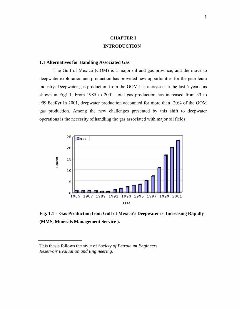
The Gulf of Mexico (GOM) is a major oil and gas province, and the move to

deepwater exploration and production has provided new opportunities for the petroleum

industry. Deepwater gas production from the GOM has increased in the last 5 years, as

shown in Fig1.1, From 1985 to 2001, total gas production has increased from 33 to

999 Bscf/yr In 2001, deepwater production accounted for more than 20% of the GOM

gas production. Among the new challenges presented by this shift to deepwater

operations is the necessity of handling the gas associated with major oil fields.

Fig. 1.1 - Gas Production from Gulf of Mexico’s Deepwater is Increasing Rapidly

(MMS, Minerals Management Service ).

This thesis follows the style of Society of Petroleum Engineers Reservoir Evaluation and Engineering.

0

5

10

15

20

25

Perc

ent

1 985 1987 1989 1991 1 993 1995 1997 1999 2001

Y ear

g a s

2

In a deepwater setting, oil can be produced and then be transported via tanker

from floating structures, however for the associated gas must also be handled in some

manner. A number of gas handling alternatives are available. These include:

• Pipeline Transportation - conventional single-phase gas pipeline or a

multiphase pipeline where the gas is combined with produced oil;

• Gas Injection - injection into the producing reservoir or injection into a

nearby or uphole aquifer;

• Liquefied Natural Gas (LNG) and transportation to shore via tanker;

• Gas to Liquids (GTL) and transportation to shore via ship or tanker;

• Compressed Natural Gas (CNG) and transportation to shore via ship;

• Gas to Wire (GTW) – offshore generation of electricity for transmission

to shore via high voltage subsea cables;

• Gas to Solids (GTS) - conversion to solid forms such as hydrates for

transport to shore via ship; and

• Lease Use - conversion to other forms of energy for use offshore in the

operation of the producing field.

Tapia1 developed economic models to compare these alternatives. His results

showed that, for a field located at water depth less than 10,000 ft and at a distance less

than 200 miles from existing facilities, a pipeline is the most profitable gas

transportation option. However, CNG and GTL are economic alternatives when gas

productions rates are greater than 110 MMscf/D. LNG is an economic alternative where

gas rates greater than 400 MMscf/D.

The objective of this study was to investigate the gas injection as an alternative

for handling the associated gas produced from the deepwater oil developments.

3

1.2.Aquifer Gas Storage

For some deepwater fields, particularly those with small gas reserves or those in

remote location, a pipelines is not economically viable. When gas can not be flared , the

usage has to be deferred, and gas may be injected into an underground storage reservoir

or producing reservoir

For the gas injection option, two alternatives are (1) injection into the producing

reservoir and (2) injection into a nearby or uphole aquifer. While injection into the

producing reservoir provides pressure support, the effect of gas reinjection on oil

production is often difficult to predict. Reservoir heterogeneity can result in rapid gas

breakthrough, in which case gas cycling can reduce efficiencies and decrease oil

production. This paper considers the case of gas injection into an aquifer and not the

producing reservoir

USA maximum working gas in storage was approximate 3,121 Bcf in 2002

according to EIA(Energy Information Administration) estimates. Aquifer gas storage is a

mature industry in USA since 1960’s. Gas storage is used to balance USA market

demand. Natural gas is injected into the aquifers in the summer when demand falls

below the supply, and it is withdrawn from storage to provide steady supply in winter,

when demand is high.

Aquifer gas storage offers possibilities for large volumes of gas to be trapped and

unrecovered. This trapped gas results when water encroaches into the pore space

previously occupied by gas. For seasonal aquifer gas storage, the first cycle is very

inefficient because of gas is trapped in the aquifer, but for the following season, it is

going more efficient, because almost all the injected gas can be produced. There are

many technical paper about aquifer gas storage, one of these example is from Coat

(Fig.2.1)

4

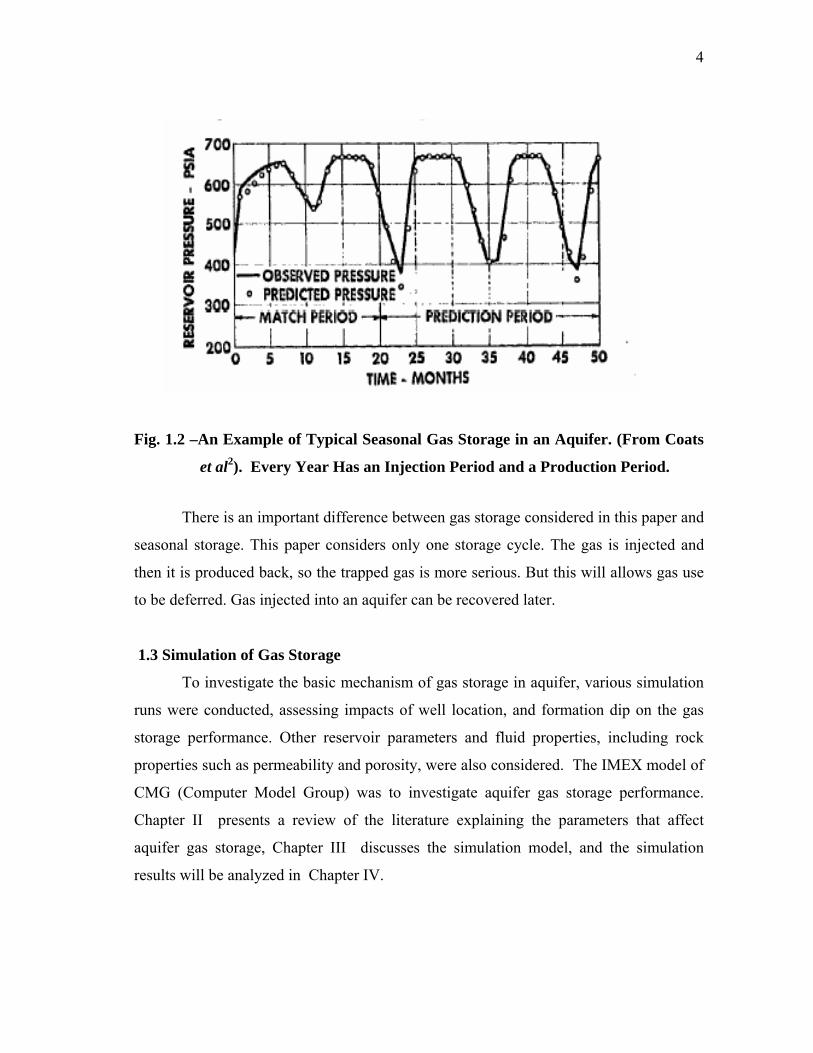
Fig. 1.2 –An Example of Typical Seasonal Gas Storage in an Aquifer. (From Coats

et al2). Every Year Has an Injection Period and a Production Period.

There is an important difference between gas storage considered in this paper and

seasonal storage. This paper considers only one storage cycle. The gas is injected and

then it is produced back, so the trapped gas is more serious. But this will allows gas use

to be deferred. Gas injected into an aquifer can be recovered later.

1.3 Simulation of Gas Storage

To investigate the basic mechanism of gas storage in aquifer, various simulation

runs were conducted, assessing impacts of well location, and formation dip on the gas

storage performance. Other reservoir parameters and fluid properties, including rock

properties such as permeability and porosity, were also considered. The IMEX model of

CMG (Computer Model Group) was to investigate aquifer gas storage performance.

Chapter II presents a review of the literature explaining the parameters that affect

aquifer gas storage, Chapter III discusses the simulation model, and the simulation

results will be analyzed in Chapter IV.

5

Few papers in the petroleum literature have reported the effects of various

parameters on the performance of aquifer storage reservoirs. So far, no study has

reported simulations of deepwater aquifer gas storage in Gulf of Mexico. Thus, a study

was needed to determine the reservoir impact of gas injection and to define generic

outputs that affect gas storage performance in deepwater aquifers.

1.4. Trapped Gas Saturation and Hysteresis

When producing the stored gas, hysteresis occurs in the relative permeability,

which results in trapped gas. This trapped gas cannot be recovered, because it doesn’t

flow. The trapped gas saturation analysis, the second stage of this study, dealt with

assessing recoverable gas from an aquifer gas storage reservoir.

In this project, the gas trapping mechanisms are described, and various empirical

correlation of Sgr vs. Sgi were investigated and compared. The hysteresis in relative

permeability options in the reservoir simulator were also investigated in this project.

1.5. Overview of Research and Study Objectives

The purposes of this project were to (1) conduct a simulation study to investigate

the effects of reservoir and well parameters on gas storage performance, (2) assess the

drainage and imbibition processes in aquifer gas storage, (3) evaluate the methods used

to determine relative permeability and residual gas saturation, and (4) gain experience

and confidence in the hysteresis option in CMG for determining the trapped gas

saturation. This project gives an up-to-date analysis of numerical simulation of the

hysteresis phenomenon, and it reports the correlation between relative permeability and

gas saturation.

6

CHAPTER II

LITERATURE REVIEW

In this chapter, a review of literature concerning alternative methods of handling

associated gas was presented and the basic mechanism of an aquifer gas storage

reservoir. In addition, residual gas saturation and relative permeability hysteresis are

reviewed.

2.1. Handling of Associated Gas

Flaring of associated gas has been recognized both as wasteful of a potentially

valuable resource and as an environmentally undesirable practice. Therefore, gas

handling in deepwater of GOM has been of great concern.

The alternatives for handling associated gas include: export via pipeline; gas

injection for later recovery; processes such as LNG, GTL, CNG and export via shuttle

tanker; conversion to products (e.g. methanol) for transport via ship; generation of

electricity for transmission to shore; and conversion to other forms of energy for use

offshore or transport to shore.

A number of economic models are being developed to comparison these various

alternative,3,4,5,6 The economic models seek to capture the performance of the various

gas handling options and to allow their comparison on the basis of their impact on

project economics and conservation of natural resources. Factors such as size of

resource, gas rate, water depth, pressure (separator & reservoir), gas composition,

temperature, etc. must be considered when comparing the various alternatives. In

addition to economic parameters, many nations are concerned about conservation of

natural resources. Processes that utilize a large percentage of the produced gas to

bringing the gas to market are less desirable.

7

2.2. Gas Storage in Aquifers

Since the early 1960’s, aquifer gas storage fields have been developed in many

parts of the USA. Gas storage is playing an increasingly important role in gas supply

management. Natural gas is injected during summer when supply exceeds demand, and

it is withdrawn in the winter to meet the market needs. The prospective deepwater site

modeled for gas storage in this study is a blanket water-bearing sand in an anticlinal

structure7

Aquifer storage now accounts for about 22% of the total gas storage capacity in

the USA. Most of the saline aquifer storage fields are in the mid-continent area. Walter

et al8 presented the results of a simulation study of one such field, the Sciota aquifer gas

storage field in Illinois. This field has been in operation since early 1970’s and is

currently operating with 12 injecting wells and five observation wells.

There have been many technical papers about the performance of the gas storage

reservoirs. For example, Coats, et al2 described the interaction between the gas storage

and the aquifer pressure behavior, and Kuncir et al9 presented two studies of the size

impact and data uncertainty on aquifer gas storage.

2.2.1 Parameters Affecting Gas Storage Reservoir

The basic parameters affecting the performance of an aquifer gas storage

reservoir are aquifer size, structure, and thickness of the storage zone. Also important are

rock properties, such as permeability and porosity, and fluid properties, including

relative permeability and capillary pressure.

Several papers discussed the experimental studies of the basic mechanisms of

aquifer gas storage at a reservoir pore scale. Briggs and Katz10 conducted an

experimental and simulation study on the mechanism of the drainage of water from sand

8

in developing aquifer gas storage. Their experimental results demonstrated three

characteristics of aquifer gas storage.

Gober11 made a qualitative analysis of the parameters affecting aquifer storage,

such as boundary conditions, well completions, overpressure, and cyclic two-phase flow.

However, they didn’t conduct a numerical reservoir simulation or experimental study of

the effects of these factors on the performance of an aquifer gas storage reservoir.

2.2.2 Gas Storage Simulation

The complexity of a real reservoirs makes it nearly impossible to conduct a

comprehensive investigation of all these parameters in a simulation study. Only a few

papers tried to address the effects of various parameter on aquifer gas storage.

Arastoopour and Chen12 performed a sensitivity analysis of the primary reservoir

parameters using a 3D numerical simulation model of a tight gas reservoir. They studied

the effects of absolute permeability, porosity, and capillary pressure on the production of

gas from single well. Their study showed that production rates, particularly gas

production rates are sensitive to both the absolute permeability and the relative

permeability.

Kuuskraa and Wicks13 (1992) published a simulation investigation of the

geologic and reservoir mechanisms controlling gas recovery from the Antrim shale.

Their parametric sensitivity study of the field included: fracture spacing, porosity, gas

sorption time, rock compressibility, absolute and relative permeability, and skin. This

study, which was done using COMEPT-3D reservoir simulator, showed that absolute

permeability has a large effect on the gas production rate. They also found that relative

permeability is equally as important as absolute permeability in affecting gas production

rate.

9

Wang14 made a parametric simulation study and also conducted a history match

of an actual gas storage aquifer. And his simulation study shows that the formation

permeability is the most important parameter affecting the cumulative gas recovery. And

the formation dip angle and porosity are of second-order importance in affecting the

cumulative gas recovery.

2.3. Residual Gas Saturation

The residual gas saturation (Sgr) is always used to estimate recovery from aquifer

gas storage reservoirs. Various methods are available for predicting the residual gas

saturation. Geffen15 et al measured residual gas saturation of 15 to 50 percent the pore

space for various porous media. They investigated the factors that affect the residual gas

saturation, such as flooding rate, static pressure, temperature, sample size, and saturation

conditions before flooding. Their results indicated that the residual gas saturation could

be 35 percent of pore volume in the actual field situation.

Naar and Henderson,16 on the other hand, concluded that residual nonwetting

phase saturation under imbibition should be about half the initial non-wetting phase

saturation.

Keelan and Pugh17 concluded that trapped gas saturation existed after gas

displacement by wetting-phase imbibition in carbonate reservoirs. Their experiments

showed that the trapped gas varied with initial gas in place and that it was a function of

rock type.

Agarwal 18 addressed the relationship between initial and final gas saturation

from an experimental perspective. He worked with data from data from 320 imbibition

experiments. Multiple regression analysis techniques were used by rock type. Four

different sets of data were obtained. These included: (1) consolidated sandstones; (2)

limestones; (3) unconsolidated sandstones; and (4) unconsolidated sands. Agarwal’s

10

results show that it is impossible to develop a general correlation of high accuracy.

However, established relationships can provide estimates of the residual gas saturation

when laboratory data are unavailable.

In 1967, building on work of Naar and Agarwal, Land19 proposed a relationship

between the residual gas saturation (Sgr) and the maximum historical gas saturation.( Sgi )

established during the drainage process. Land20 later experimentally verified the model

by comparing the calculated with experimental imbibition relative permeability. The

stationary-liquid-phase method was used to measure several hysteresis loops for

alundum and Berea sandstone samples, and a good match was observed.

Recently, various empirical Sgrand Sgi relationship21,22,23,24,25 were proposed.

Most of them are based on limited experimental results. However, two of these

relationships gained popularity because of the supporting experimental data.

First, Jerauld23 worked on fifty Berea and Prudhoe Bay sandstone samples, and

proposed the hyperbolic form the relationship. Aissaouir25 demonstrated a piecewise

linear relationship with two parameters: Sgrm and Sgo. Sgo is the saturation corresponding

to the intersection of the two segments. Aissaoui’s work is based on twelve

Fontainebleau sandstone plugs. Later, Suzane21 worked on sixty experimental Sgr- Sgi

plugs, and the experimental results showed that the Aissaoui’sempirical relationship best

describe her data set.

2.4. Extension of Previous Work

Only a few of the published studies have investigated some of the basic

mechanisms controlling the behavior of an aquifer gas storage reservoir. A

comprehensive simulation study of the effects of the various combinations of the

primary reservoir parameters on performance of and aquifer gas storage reservoir was

not found. There are also very few papers that discuss residual gas saturation

11

determination and hysteresis in CMG. Two main objectives of this research are to (1)

study the factors that affect gas storage in an aquifer by comprehensively investigating

the effects of the primary parameters on the dynamic performance, and (2) investigate

the hysteresis option in CMG. These objectives were accomplished by making

simulation runs for all the representative value combinations of the primary reservoir

parameters and conducting a comprehensive analysis of the methods of residual gas

determination of the aquifer gas storage reservoir in reservoir scale.

12

CHAPTER III

CONSTRUCTION OF THE RESERVOIR MODEL

To conduct a simulation study, it was necessary to choose a simulator and to

create a geologic model. The first step preparing the simulation cases was to determine

the representative values of the main parameters, which should reflect reservoir

characteristics and operational condition in a hypothetical aquifer gas storage field.

3.1 Description of the Simulators

For this study, a simulation software owned by Computer Modeling Group Ltd is

used. IMEX is a black oil simulator in CMG. It models three phases fluid in gas, gas-

water, oil-water reservoir in one, two, or three dimensions. IMEX models multiple PVT

and equilibrium regions, as well as multiple rock types, and it has flexible relative

permeability choices.

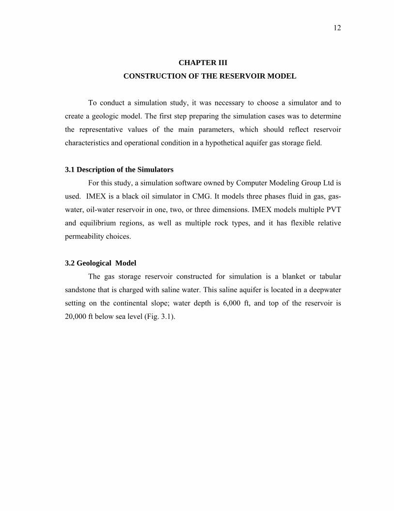
3.2 Geological Model

The gas storage reservoir constructed for simulation is a blanket or tabular

sandstone that is charged with saline water. This saline aquifer is located in a deepwater

setting on the continental slope; water depth is 6,000 ft, and top of the reservoir is

20,000 ft below sea level (Fig. 3.1).

13

Fig. 3.1 - Schematic of the Modeled Field Areas.

Structurally, the model is an anticline that plunges 20º from the center, front edge

of the model toward the back of the block (Fig. 3.2). The plunge is constant along the

axis, on the right and left flanks of the symmetrical anticline are 10º. Crestal elevation of

the model is 20,000 ft below sea level (Fig. 3.1). Elevation of the anticlinal crest is –

22,655 ft at the rear of the block. The boundaries of the block are inferred to be no-flow

boundaries in the reservoir model, owing to presence of faults or sandstone pinch-outs.

Sealing horizons overlie and underlie the sandstone aquifer. For this model, I inferred

that reservoir properties of the tabular sandstone are homogeneous. Reservoir porosity is

20% and permeability is 300 md.

Aq

20,000 ft

6,00

Aquifer

Sealing Fault

SL

14

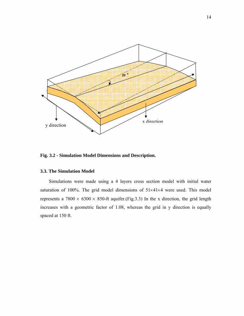
Fig. 3.2 - Simulation Model Dimensions and Description.

3.3. The Simulation Model

Simulations were made using a 4 layers cross section model with initial water

saturation of 100%. The grid model dimensions of 51×41×4 were used. This model

represents a 7800 × 6300 × 850-ft aquifer.(Fig.3.3) In the x direction, the grid length

increases with a geometric factor of 1.08, whereas the grid in y direction is equally

spaced at 150 ft.

20 º

y direction x direction

15

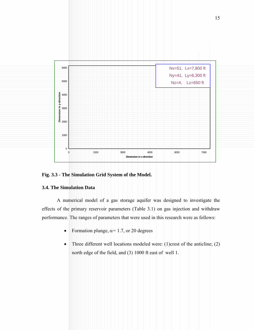
Fig. 3.3 - The Simulation Grid System of the Model.

3.4. The Simulation Data

A numerical model of a gas storage aquifer was designed to investigate the

effects of the primary reservoir parameters (Table 3.1) on gas injection and withdraw

performance. The ranges of parameters that were used in this research were as follows:

• Formation plunge, α= 1.7, or 20 degrees

• Three different well locations modeled were: (1)crest of the anticline; (2)

north edge of the field, and (3) 1000 ft east of well 1.

0

1000

2000

3000

4000

5000

6000

0 1500 3000 4500 6000 7500

Dimension in x-direction

Dim

ensi

on in

y-d

irect

ion

Nx=51, Lx=7,800 ft

Ny=41, Ly=6,300 ft

Nz=4, Lz=650 ft

16

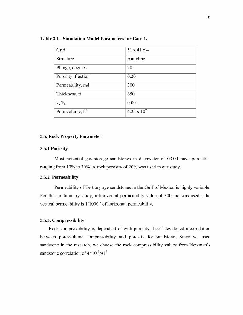
Table 3.1 - Simulation Model Parameters for Case 1.

3.5. Rock Property Parameter

3.5.1 Porosity

Most potential gas storage sandstones in deepwater of GOM have porosities

ranging from 10% to 30%. A rock porosity of 20% was used in our study.

3.5.2 Permeability

Permeability of Tertiary age sandstones in the Gulf of Mexico is highly variable.

For this preliminary study, a horizontal permeability value of 300 md was used ; the

vertical permeability is 1/1000th of horizontal permeability.

3.5.3. Compressibility

Rock compressibility is dependent of with porosity. Lee27 developed a correlation

between pore-volume compressibility and porosity for sandstone, Since we used

sandstone in the research, we choose the rock compressibility values from Newman’s

sandstone correlation of 4*10-6psi-1

Grid 51 x 41 x 4

Structure Anticline

Plunge, degrees 20

Porosity, fraction 0.20

Permeability, md 300

Thickness, ft 650

kv/kh 0.001

Pore volume, ft3 6.25 x 109

17

3.6. Reservoir Parameters

3.6.1. Formation Dip

Formation dip is an important parameter in determining the gas recovery in

aquifer storage reservoirs. Dip varies in structural setting of different aquifers, and

commonly, it varies in different part of and individual aquifer. For our simulation runs,

twodip values of 1.7 and 20 were used, these value will represent the range in dip of

most aquifer gas storage fields. The highest point of the aquifer is 20,000 feet. The

elevation of each of the cell of the gridblock would be given by the formula .

⎟⎟

⎠

⎞

⎜⎜

⎝

⎛ −++=

Totalwidth

2yDeltaryGridboundaθ20,000Elevation

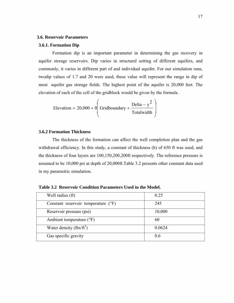
3.6.2 Formation Thickness

The thickness of the formation can affect the well completion plan and the gas

withdrawal efficiency. In this study, a constant of thickness (h) of 650 ft was used, and

the thickness of four layers are 100,150,200,200ft respectively. The reference pressure is

assumed to be 10,000 psi at depth of 20,000ft.Table 3.2 presents other constant data used

in my parametric simulation.

Table 3.2 Reservoir Condition Parameters Used in the Model.

Well radius (ft) 0.25

Constant reservoir temperature (°F) 245

Reservoir pressure (psi) 10,000

Ambient temperature (°F) 60

Water density (lbs/ft3) 0.0624

Gas specific gravity 0.6

18

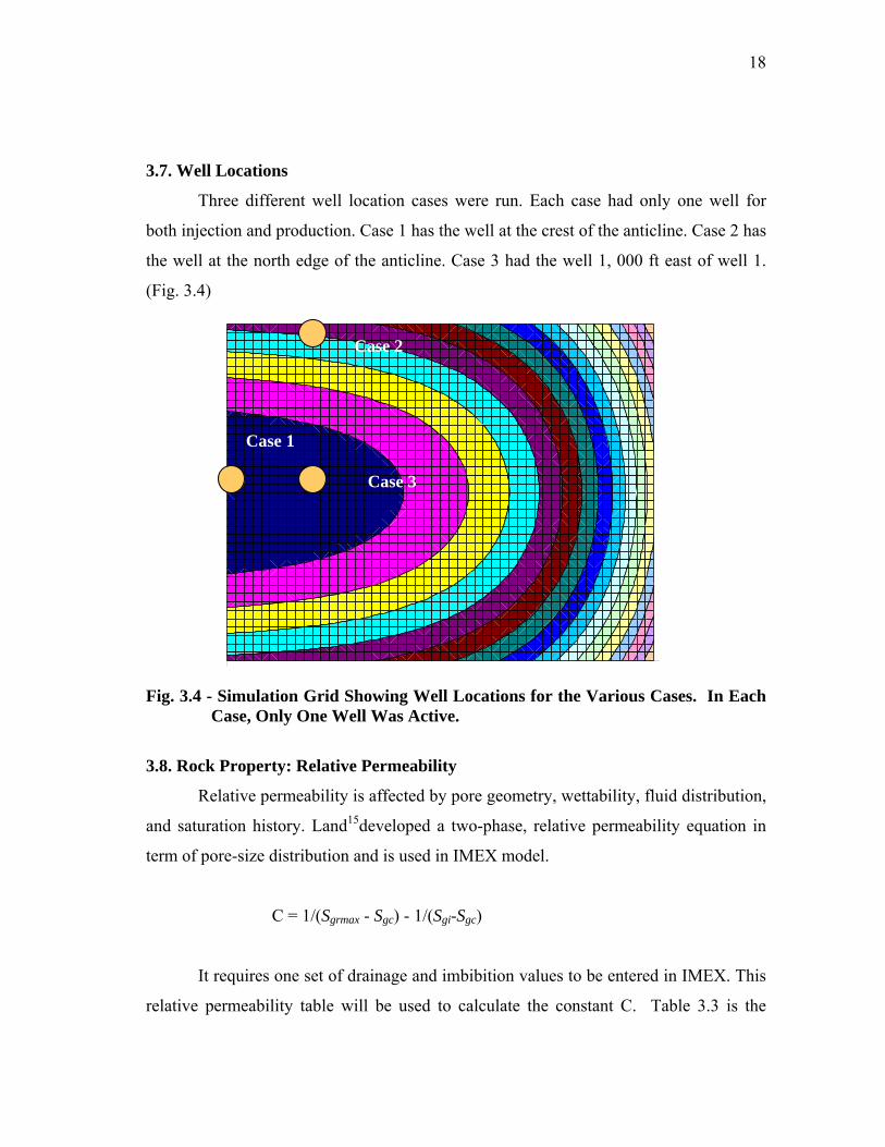
3.7. Well Locations

Three different well location cases were run. Each case had only one well for

both injection and production. Case 1 has the well at the crest of the anticline. Case 2 has

the well at the north edge of the anticline. Case 3 had the well 1, 000 ft east of well 1.

(Fig. 3.4)

Fig. 3.4 - Simulation Grid Showing Well Locations for the Various Cases. In Each

Case, Only One Well Was Active.

3.8. Rock Property: Relative Permeability

Relative permeability is affected by pore geometry, wettability, fluid distribution,

and saturation history. Land15developed a two-phase, relative permeability equation in

term of pore-size distribution and is used in IMEX model.

C = 1/(Sgrmax - Sgc) - 1/(Sgi-Sgc)

It requires one set of drainage and imbibition values to be entered in IMEX. This

relative permeability table will be used to calculate the constant C. Table 3.3 is the

Case 1

Case 3

Case 2

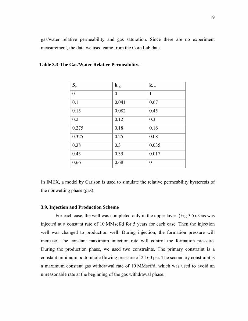
19

gas/water relative permeability and gas saturation. Since there are no experiment

measurement, the data we used came from the Core Lab data.

Table 3.3-The Gas/Water Relative Permeability.

In IMEX, a model by Carlson is used to simulate the relative permeability hysteresis of

the nonwetting phase (gas).

3.9. Injection and Production Scheme

For each case, the well was completed only in the upper layer. (Fig 3.5). Gas was

injected at a constant rate of 10 MMscf/d for 5 years for each case. Then the injection

well was changed to production well. During injection, the formation pressure will

increase. The constant maximum injection rate will control the formation pressure.

During the production phase, we used two constraints. The primary constraint is a

constant minimum bottomhole flowing pressure of 2,160 psi. The secondary constraint is

a maximum constant gas withdrawal rate of 10 MMscf/d, which was used to avoid an

unreasonable rate at the beginning of the gas withdrawal phase.

Sg krg krw

0 0 1

0.1 0.041 0.67

0.15 0.082 0.45

0.2 0.12 0.3

0.275 0.18 0.16

0.325 0.25 0.08

0.38 0.3 0.035

0.45 0.39 0.017

0.66 0.68 0

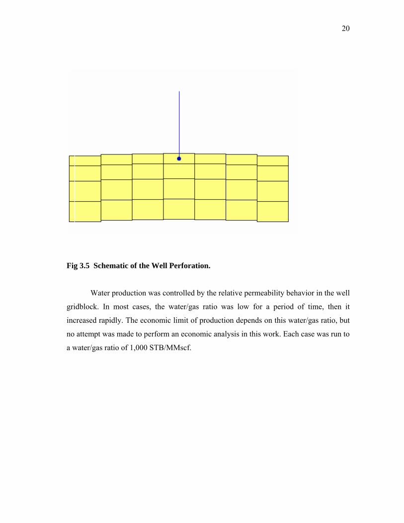
20

Fig 3.5 Schematic of the Well Perforation.

Water production was controlled by the relative permeability behavior in the well

gridblock. In most cases, the water/gas ratio was low for a period of time, then it

increased rapidly. The economic limit of production depends on this water/gas ratio, but

no attempt was made to perform an economic analysis in this work. Each case was run to

a water/gas ratio of 1,000 STB/MMscf.

21

CHAPTER IV

SIMULATION RESULTS AND DISCUSSION

For this study, a numerical model of a hypothetical gas storage aquifer was

designed to investigate the effects of primary reservoir parameters and the gas injection

and withdrawal scheme on the performance of aquifer gas storage reservoir. The focus

was on the effects of formation dip and well location. The results of the simulation cases

are summarized in the following sections.. More details are shown for Case 1, since it is

the most favorable case.

4.1. Effect of Formation Dip

Formation dip angle is an important parameter for aquifer gas storage. In this

project, Two cases were run. One has a dip angle of 1.7 degree, whereas the others has a

dip of 20 degrees.

The simulation results show that the case with a higher dip favors gas trapping

near the crest of the anticline. Owing to the gravity difference of gas and water, the gas

more readily migrates up dip in the structure having the greatest dip, and it forms a gas

cap around the top of structure. Table 4.1 shows the effects of formation dip angle on the

cumulative gas production .

22

Table 4.1 Simulation Result Showing Effect of Dip on Reservoir Performance.

4.2 Effect of Well Location on Aquifer Gas Storage Performance

Based on the previous simulation result, I choose dip angle of 20 for the next

cases. Three cases were run to test the effects of well location on aquifer gas storage

reservoir performance. Case 1 has the well at the crest of the anticline. Case 2 has the

well at the north edge of the anticline, and case 3 had the well 1,000 ft east of well 1.

The total gas injected for each case is 18.27 Bscf in 5 years.

Case 1 Case1a (Plunge=1.7) Plungedegree 20

1.7

Total gas injection (Bscf) 18,3 18.3

Total gas production (Bscf) 7.1 5.6

Total water production (MSTB)

18.2 906.6

Recovery (%)

39.1 30.8

Project life (years) 7.0 6.5

23

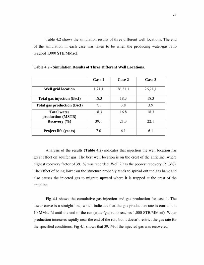
Table 4.2 shows the simulation results of three different well locations. The end

of the simulation in each case was taken to be when the producing water/gas ratio

reached 1,000 STB/MMscf.

Table 4.2 - Simulation Results of Three Different Well Locations.

Analysis of the results (Table 4.2) indicates that injection the well location has

great effect on aquifer gas. The best well location is on the crest of the anticline, where

highest recovery factor of 39.1% was recorded. Well 2 has the poorest recovery (21.3%).

The effect of being lower on the structure probably tends to spread out the gas bank and

also causes the injected gas to migrate upward where it is trapped at the crest of the

anticline.

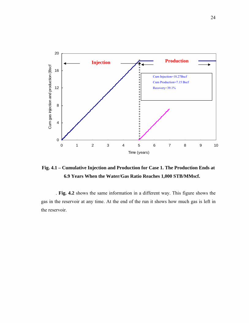
Fig 4.1 shows the cumulative gas injection and gas production for case 1. The

lower curve is a straight line, which indicates that the gas production rate is constant at

10 MMscf/d until the end of the run (water/gas ratio reaches 1,000 STB/MMscf). Water

production increases rapidly near the end of the run, but it doesn’t restrict the gas rate for

the specified conditions. Fig 4.1 shows that 39.1%of the injected gas was recovered.

Case 1 Case 2 Case 3

Well grid location 1,21,1 26,21,1 26,21,1

Total gas injection (Bscf) 18.3 18.3 18.3

Total gas production (Bscf) 7.1 3.8 3.9

Total water production (MSTB)

18.3 16.8 18.3

Recovery (%)

39.1 21.3 22.1

Project life (years) 7.0 6.1 6.1

24

0

4

8

12

16

20

0 1 2 3 4 5 6 7 8 9 10

Time (years)

Cum

gas

inje

ctio

n an

d pr

oduc

tion

(Bsc

f)

Fig. 4.1 – Cumulative Injection and Production for Case 1. The Production Ends at

6.9 Years When the Water/Gas Ratio Reaches 1,000 STB/MMscf.

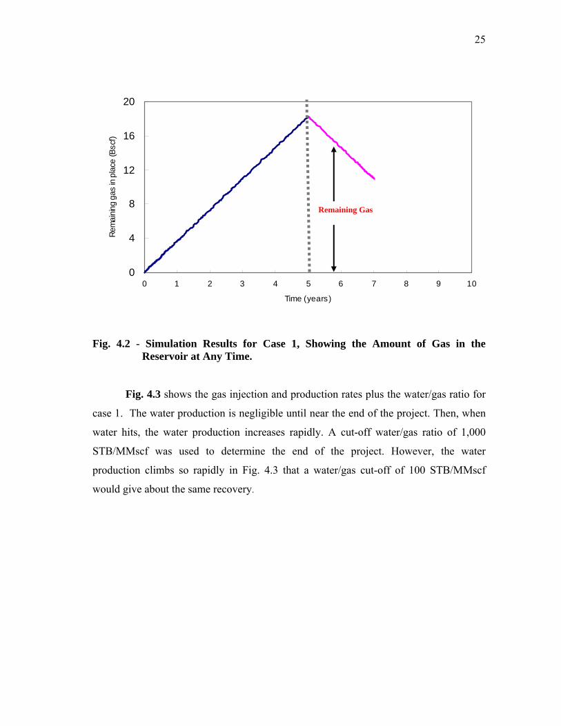
. Fig. 4.2 shows the same information in a different way. This figure shows the

gas in the reservoir at any time. At the end of the run it shows how much gas is left in

the reservoir.

Cum Injection=18.27Bscf

Cum Production=7.15 Bscf

Recovery=39.1%

Injection Production

25

Fig. 4.2 - Simulation Results for Case 1, Showing the Amount of Gas in the Reservoir at Any Time.

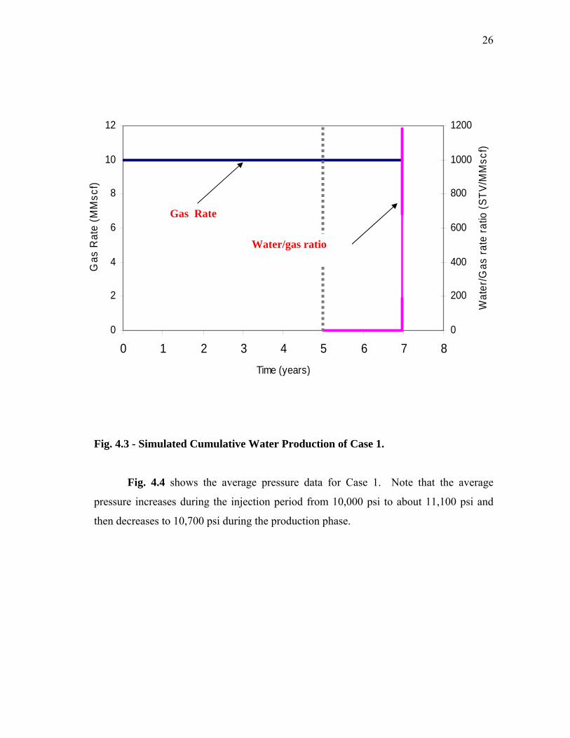
Fig. 4.3 shows the gas injection and production rates plus the water/gas ratio for

case 1. The water production is negligible until near the end of the project. Then, when

water hits, the water production increases rapidly. A cut-off water/gas ratio of 1,000

STB/MMscf was used to determine the end of the project. However, the water

production climbs so rapidly in Fig. 4.3 that a water/gas cut-off of 100 STB/MMscf

would give about the same recovery.

0

4

8

12

16

20

0 1 2 3 4 5 6 7 8 9 10

Time (years)

Rem

ainin

g ga

s in

pla

ce (B

scf)

Remaining Gas

26

Fig. 4.3 - Simulated Cumulative Water Production of Case 1.

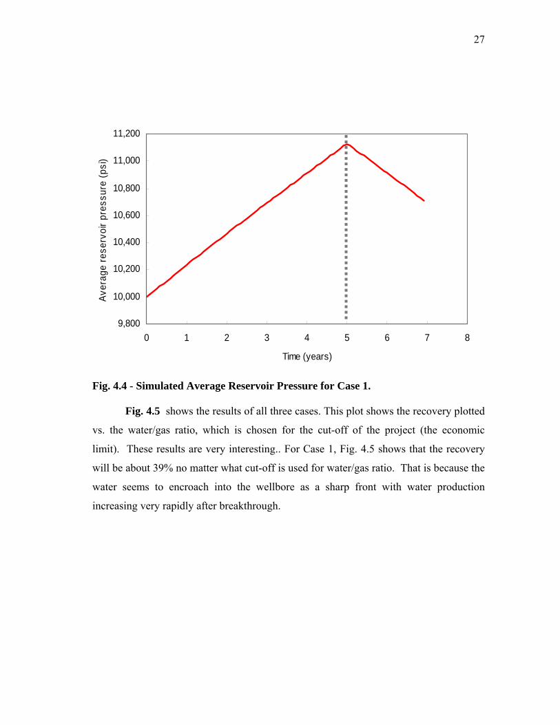
Fig. 4.4 shows the average pressure data for Case 1. Note that the average

pressure increases during the injection period from 10,000 psi to about 11,100 psi and

then decreases to 10,700 psi during the production phase.

0

2

4

6

8

10

12

0 1 2 3 4 5 6 7 8Time (years)

Gas

Rat

e (M

Msc

f)

0

200

400

600

800

1000

1200

Wat

er/G

as ra

te ra

tio (S

TV/M

Msc

f)

Gas Rate

Water/gas ratio

27

Fig. 4.4 - Simulated Average Reservoir Pressure for Case 1.

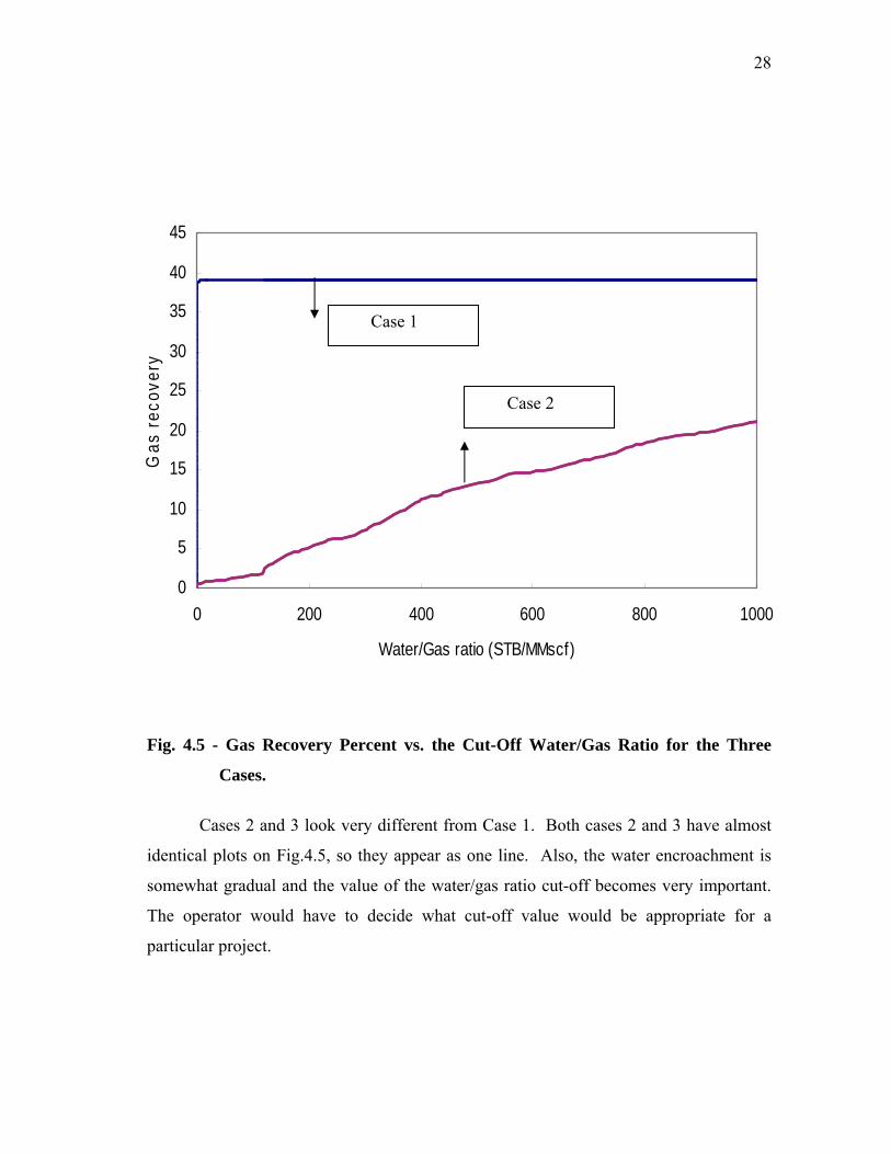
Fig. 4.5 shows the results of all three cases. This plot shows the recovery plotted

vs. the water/gas ratio, which is chosen for the cut-off of the project (the economic

limit). These results are very interesting.. For Case 1, Fig. 4.5 shows that the recovery

will be about 39% no matter what cut-off is used for water/gas ratio. That is because the

water seems to encroach into the wellbore as a sharp front with water production

increasing very rapidly after breakthrough.

9,800

10,000

10,200

10,400

10,600

10,800

11,000

11,200

0 1 2 3 4 5 6 7 8

Time (years)

Aver

age

rese

rvoi

r pre

ssur

e (p

si)

28

Fig. 4.5 - Gas Recovery Percent vs. the Cut-Off Water/Gas Ratio for the Three

Cases.

Cases 2 and 3 look very different from Case 1. Both cases 2 and 3 have almost

identical plots on Fig.4.5, so they appear as one line. Also, the water encroachment is

somewhat gradual and the value of the water/gas ratio cut-off becomes very important.

The operator would have to decide what cut-off value would be appropriate for a

particular project.

0

5

10

15

20

25

30

35

40

45

0 200 400 600 800 1000

Water/Gas ratio (STB/MMscf)

Gas

reco

very

Case 1

Case 2

29

CHAPTER V

RESIDUAL GAS SATURATION AND RELATIVE

PERMEABILITY HYSTERESIS

Trapped gas saturation, the second phase of our study, dealt with assessing

recoverable gas in aquifer gas storage. Residual gas saturation is known to be dependent

on both pore network characteristics and initial gas saturation. The economic impact of

residual gas saturation (Sgr) on aquifer gas storage can be very high.

Many methods are available to estimate residual gas saturation. In this chapter,

the gas-trapping mechanisms are described and the correlations developed by Naar and

Henderson, Agarwal , Land, Aissaoui, Kleppe, Jerauld, were presented and compared.

The methods of calculating imbibition relative permeability is described, and

experimental calculated and simulated residual gas saturations are compared and they

are shown to match well.

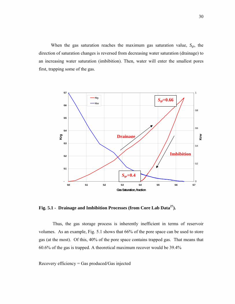
5.1. Gas Trapping Mechanism

For aquifer gas storage, the rock is initially and completely saturated with the

wetting phase. For the problem addressed in this project, the wetting phase is assumed to

be water, and nonwetting phase is assumed to be gas. When the gas is injected, the water

is displaced by the gas, and the water saturation is reduced until critical gas saturation is

reached. At this point, the gas begins to flow. As the Sg increases, the relative

permeability of gas also increases. Gas enters the largest pore size first, and then invades

the smaller and smaller pores (Fig. 5.1).

30

When the gas saturation reaches the maximum gas saturation value, Sgi, the

direction of saturation changes is reversed from decreasing water saturation (drainage) to

an increasing water saturation (imbibition). Then, water will enter the smallest pores

first, trapping some of the gas.

Fig. 5.1 - Drainage and Imbibition Processes (from Core Lab Data27).

Thus, the gas storage process is inherently inefficient in terms of reservoir

volumes. As an example, Fig. 5.1 shows that 66% of the pore space can be used to store

gas (at the most). Of this, 40% of the pore space contains trapped gas. That means that

60.6% of the gas is trapped. A theoretical maximum recover would be 39.4%

Recovery efficiency = Gas produced/Gas injected

-

0.1

0.2

0.3

0.4

0.5

0.6

0.7

0.0 0.1 0.2 0.3 0.4 0.5 0.6 0.7

Gas Saturation, fraction

Krg

0

0.2

0.4

0.6

0.8

1

Krw

Krg

Krw

Imbibition

Drainage

Sgi=0.66

Sgr=0.4

31

= ( %4.390664466

=−− )

For parts of the reservoir which do not reach the maximum value of 66% gas

saturation, the trapped gas percentage is even higher. An additional factor in determining

the efficiency of gas storage is the high water cuts that can limit production long before

the residual gas saturation is reached.

5.2. Residual Gas Saturation Determination

Many methods are available for estimation of residual gas saturation. These

correlation attempt to use different approach to determine Sg, but none was entirely

satisfactory. Most of these methods require special core analysis to establish at least one

value for Sgr.Then, other values can be calculated for different starting values of gas

saturation. However, the first two of the following methods can be used to calculate Sgr

without special core analysis.

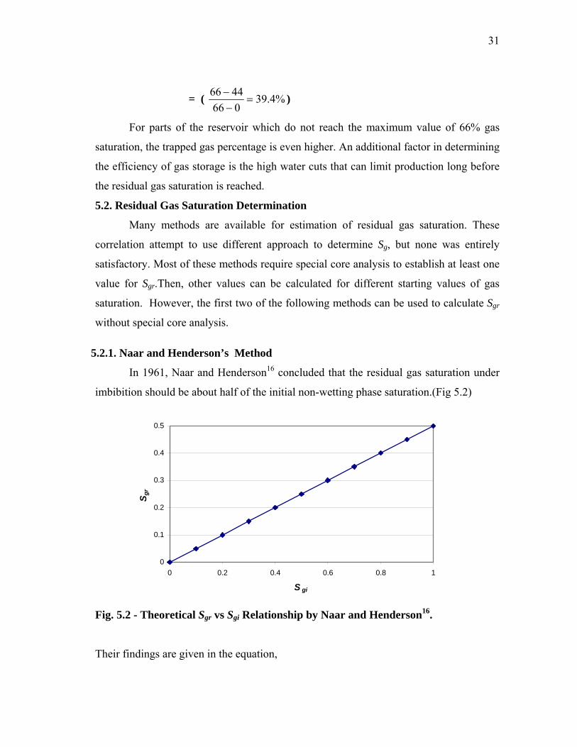
5.2.1. Naar and Henderson’s Method

In 1961, Naar and Henderson16 concluded that the residual gas saturation under

imbibition should be about half of the initial non-wetting phase saturation.(Fig 5.2)

Fig. 5.2 - Theoretical Sgr vs Sgi Relationship by Naar and Henderson16.

Their findings are given in the equation,

0

0.1

0.2

0.3

0.4

0.5

0 0.2 0.4 0.6 0.8 1

S gi

S gr

32

giSgrS21

= ………………………………………………………………………(5-1)

This method doesn’t require additional parameters, therefore, when laboratory

data are not available, and it can be a good estimate rather than an arbitrarily assumed

value.

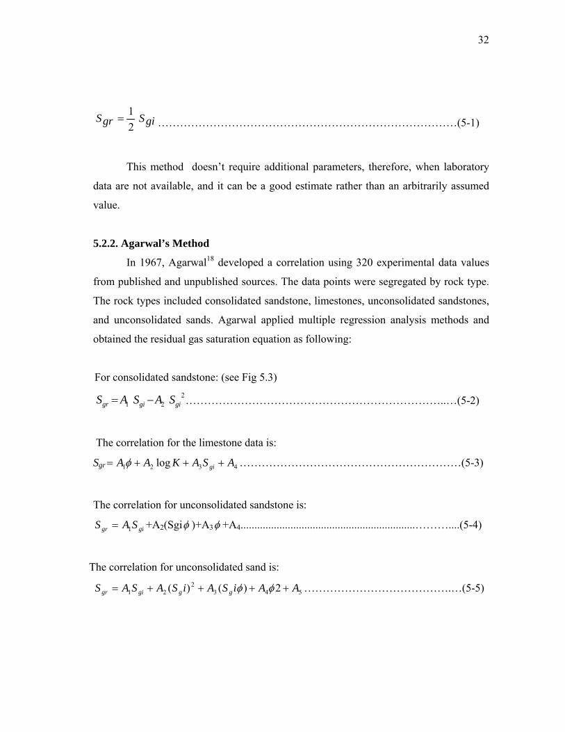
5.2.2. Agarwal’s Method

In 1967, Agarwal18 developed a correlation using 320 experimental data values

from published and unpublished sources. The data points were segregated by rock type.

The rock types included consolidated sandstone, limestones, unconsolidated sandstones,

and unconsolidated sands. Agarwal applied multiple regression analysis methods and

obtained the residual gas saturation equation as following:

For consolidated sandstone: (see Fig 5.3)

221 gigigr SASAS −= ……………………………………………………………..…(5-2)

The correlation for the limestone data is:

Sgr 4321 log ASAKAA gi +++= φ ……………………………………………………(5-3)

The correlation for unconsolidated sandstone is:

=grS giSA1 +A2(Sgiφ )+A3φ +A4...............................................................………....(5-4)

The correlation for unconsolidated sand is:

5432

21 2)()( AAiSAiSASAS gggigr ++++= φφ ………………………………….…(5-5)

33

Coefficients of the regression equation are listed in the Table 5.1

Table 5.1. Coefficients of the Regression Equations of Agarwal

A1 A2 A3 A4 A5

Eq 0.8084 -0.6386*10-2

Eq -0.5348 0.3355*10 0.1545 0.1440*102

Eq -0.5125 0.2609*10-1 -0.2676 0.14796*102

Eq 0.4936*10 -0.3004*10-1 -0.2013*102 0.1615*10-1 -0.1448*103

Fig. 5.3 – Theoretical Sgr vs Sgi Relationship of Agarwal18.

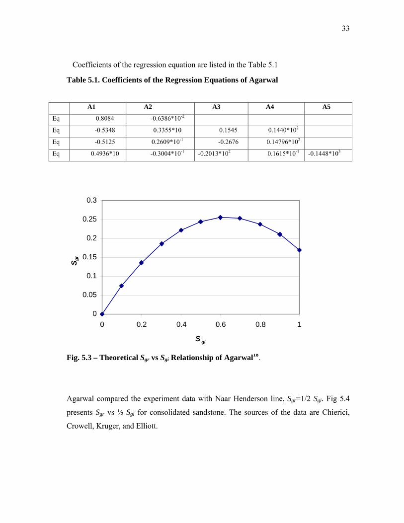
Agarwal compared the experiment data with Naar Henderson line, Sgr=1/2 Sgi. Fig 5.4

presents Sgr vs ½ Sgi for consolidated sandstone. The sources of the data are Chierici,

Crowell, Kruger, and Elliott.

0

0.05

0.1

0.15

0.2

0.25

0.3

0 0.2 0.4 0.6 0.8 1

S gi

S gr

34

Fig.5.4- Measured Sgr vs. Naar and Henderson Line for the Consolidated Sandstone

(Agarwal’s dissertation).

From the Fig. 5.4, we can see that the Crowell, Kruger and Elliott agree with the

Narr and Henderson’s line, whereas the Chierici’s data show a very different trend. In

fact, the Chierici data appear to be a separate population that exhibit no trend and falls

below the trend line exhibited by the other three populations.

Fig 5.4 shows that Sgr calculated vs. Sgr measured for the consolidated sandstone.

The Chierici data show a diversified population, and this indicates that the correlation is

not accurate and should not be used for determining the residual gas saturation.

35

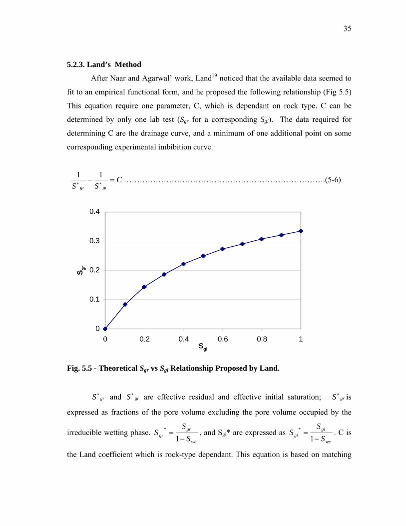
5.2.3. Land’s Method

After Naar and Agarwal’ work, Land19 noticed that the available data seemed to

fit to an empirical functional form, and he proposed the following relationship (Fig 5.5)

This equation require one parameter, C, which is dependant on rock type. C can be

determined by only one lab test (Sgr for a corresponding Sgi). The data required for

determining C are the drainage curve, and a minimum of one additional point on some

corresponding experimental imbibition curve.

CSS gigr

=− ∗∗

11 ………………………………………………………………….(5-6)

Fig. 5.5 - Theoretical Sgr vs Sgi Relationship Proposed by Land.

grS ∗ and giS ∗ are effective residual and effective initial saturation; grS ∗ is

expressed as fractions of the pore volume excluding the pore volume occupied by the

irreducible wetting phase. wc

grgr S

SS

−=

1* , and Sgi* are expressed as

wc

gigi S

SS

−=

1* . C is

the Land coefficient which is rock-type dependant. This equation is based on matching

0

0.1

0.2

0.3

0.4

0 0.2 0.4 0.6 0.8 1Sgi

S gr

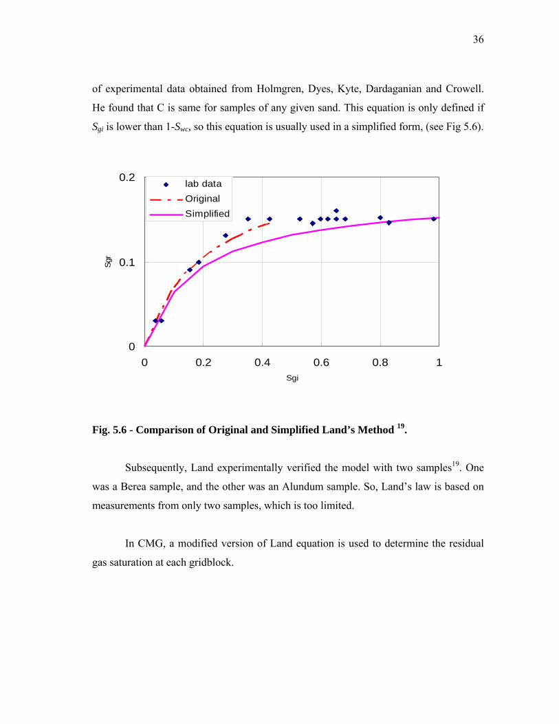
36

of experimental data obtained from Holmgren, Dyes, Kyte, Dardaganian and Crowell.

He found that C is same for samples of any given sand. This equation is only defined if

Sgi is lower than 1-Swc, so this equation is usually used in a simplified form, (see Fig 5.6).

0

0.1

0.2

0 0.2 0.4 0.6 0.8 1Sgi

Sgr

lab dataOriginalSimplified

Fig. 5.6 - Comparison of Original and Simplified Land’s Method 19.

Subsequently, Land experimentally verified the model with two samples19. One

was a Berea sample, and the other was an Alundum sample. So, Land’s law is based on

measurements from only two samples, which is too limited.

In CMG, a modified version of Land equation is used to determine the residual

gas saturation at each gridblock.

37

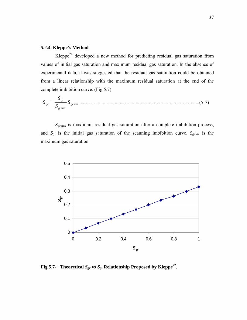
5.2.4. Kleppe’s Method

Kleppe22 developed a new method for predicting residual gas saturation from

values of initial gas saturation and maximum residual gas saturation. In the absence of

experimental data, it was suggested that the residual gas saturation could be obtained

from a linear relationship with the maximum residual saturation at the end of the

complete imbibition curve. (Fig 5.7)

max

maxgr

g

gigr S

SS

S = ………………………………………………………………...(5-7)

Sgrmax is maximum residual gas saturation after a complete imbibition process,

and Sgi is the initial gas saturation of the scanning imbibition curve. Sgmax is the

maximum gas saturation.

Fig 5.7- Theoretical Sgr vs Sgi Relationship Proposed by Kleppe22.

0

0.1

0.2

0.3

0.4

0.5

0 0.2 0.4 0.6 0.8 1

S gi

S gr

38

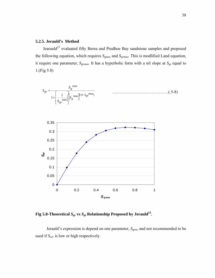
5.2.5. Jerauld’s Method

Jearauld23 evaluated fifty Berea and Prudhoe Bay sandstone samples and proposed

the following equation, which requires Sgmax and Sgrmax. This is modlified Land equation,

it require one parameter, Sgrmax. It has a hyperbolic form with a nil slope at Sgi equal to

1.(Fig 5.8)

Fig 5.8-Theoretical Sgr vs Sgi Relationship Proposed by Jerauld23.

Jerauld’s expression is depend on one parameter, Sgrm, and not recommended to be

used if Swir is low or high respectively.

[ ] )max1/(1maxmax

max

11 grSg

gr

ggr

SS

SS

−

⎥⎥

⎦

⎤

⎢⎢

⎣

⎡+

= ………………………………….(.5-8)

0

0.05

0.1

0.15

0.2

0.25

0.3

0.35

0 0.2 0.4 0.6 0.8 1

S gmax

Sgr

39

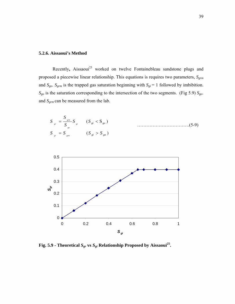
5.2.6. Aissaoui’s Method

Recently, Aissaoui25 worked on twelve Fontainebleau sandstone plugs and

proposed a piecewise linear relationship. This equations is requires two parameters, Sgrm

and Sgo. Sgrm is the trapped gas saturation beginning with Sgi = 1 followed by imbibition.

Sgo is the saturation corresponding to the intersection of the two segments. (Fig 5.9) Sgo.

and Sgrm can be measured from the lab.

Fig. 5.9 - Theoretical Sgr vs Sgi Relationship Proposed by Aissaoui25.

)(

)S( go

gogi

gi

SSSS

SSS

SS

grmgr

gi

go

grm

gr

>=

<=…………………………….(5-9)

0

0.1

0.2

0.3

0.4

0.5

0 0.2 0.4 0.6 0.8 1

S gi

S gr

40

The empirical relationship proposed was later checked by Suzanne al20, and the

experimental result show that it best describe her data set. It is a piecewise linear

relationship with two parts. And although it is more accurate, it is not recommended

because the complicated procedure to measure Sgo and Sgrm.

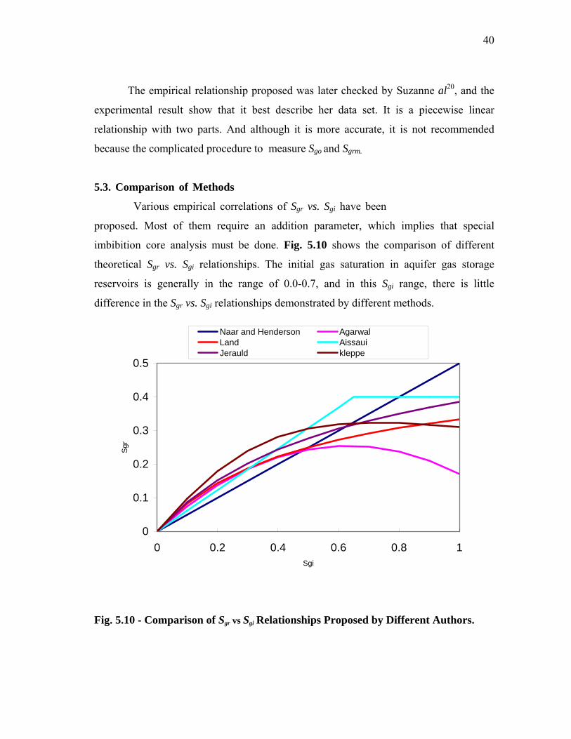
5.3. Comparison of Methods

Various empirical correlations of Sgr vs. Sgi have been

proposed. Most of them require an addition parameter, which implies that special

imbibition core analysis must be done. Fig. 5.10 shows the comparison of different

theoretical Sgr vs. Sgi relationships. The initial gas saturation in aquifer gas storage

reservoirs is generally in the range of 0.0-0.7, and in this Sgi range, there is little

difference in the Sgr vs. Sgi relationships demonstrated by different methods.

0

0.1

0.2

0.3

0.4

0.5

0 0.2 0.4 0.6 0.8 1Sgi

Sgr

Naar and Henderson AgarwalLand AissauiJerauld kleppe

Fig. 5.10 - Comparison of Sgr vs Sgi Relationships Proposed by Different Authors.

41

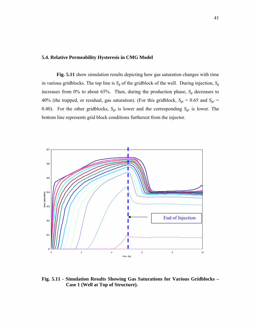
5.4. Relative Permeability Hysteresis in CMG Model

Fig. 5.11 show simulation results depicting how gas saturation changes with time

in various gridblocks. The top line is Sg of the gridblock of the well. During injection, Sg

increases from 0% to about 65%. Then, during the production phase, Sg decreases to

40% (the trapped, or residual, gas saturation). (For this gridblock, Sgi = 0.65 and Sgr =

0.40). For the other gridblocks, Sgi is lower and the corresponding Sgr is lower. The

bottom line represents grid block conditions furtherest from the injector.

Fig. 5.11 - Simulation Results Showing Gas Saturations for Various Gridblocks –

Case 1 (Well at Top of Structure).

0

0.1

0.2

0.3

0.4

0.5

0.6

0.7

0 2 4 6 8 10

time, day

Gas

sat

urat

ion

End of Injection

42

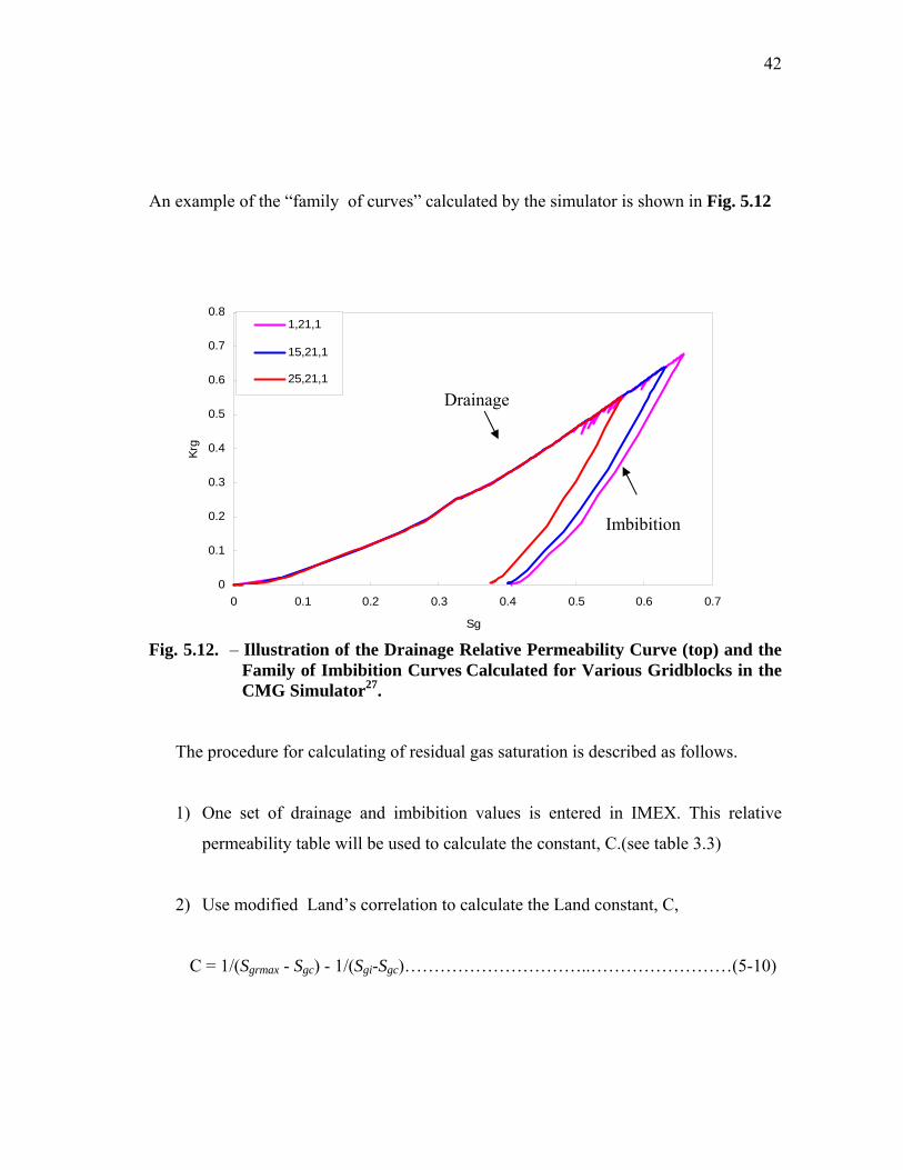
An example of the “family of curves” calculated by the simulator is shown in Fig. 5.12

Fig. 5.12. – Illustration of the Drainage Relative Permeability Curve (top) and the Family of Imbibition Curves Calculated for Various Gridblocks in the CMG Simulator27.

The procedure for calculating of residual gas saturation is described as follows.

1) One set of drainage and imbibition values is entered in IMEX. This relative

permeability table will be used to calculate the constant, C.(see table 3.3)

2) Use modified Land’s correlation to calculate the Land constant, C,

C = 1/(Sgrmax - Sgc) - 1/(Sgi-Sgc)…………………………..……………………(5-10)

0

0.1

0.2

0.3

0.4

0.5

0.6

0.7

0.8

0 0.1 0.2 0.3 0.4 0.5 0.6 0.7

Sg

Krg

1,21,1

15,21,1

25,21,1

Drainage

Imbibition

43

where Sgc is critical gas saturation, and Sgrmax is maximum residual gas saturation,

must be entered on the HYSKRG option in IMEX. It is a value obtained from an

imbibition curve from connate liquid saturation.

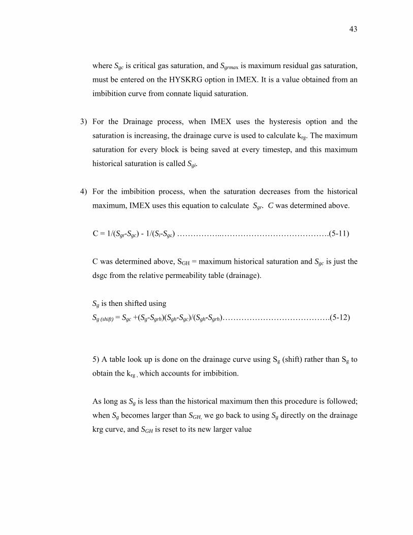
3) For the Drainage process, when IMEX uses the hysteresis option and the

saturation is increasing, the drainage curve is used to calculate krg. The maximum

saturation for every block is being saved at every timestep, and this maximum

historical saturation is called Sgi.

4) For the imbibition process, when the saturation decreases from the historical

maximum, IMEX uses this equation to calculate Sgr. C was determined above.

C = 1/(Sgr-Sgc) - 1/(Si-Sgc) ……………..………………………………….(5-11)

C was determined above, SGH = maximum historical saturation and Sgc is just the

dsgc from the relative permeability table (drainage).

Sg is then shifted using

Sg (shift) = Sgc +(Sg-Sgrh)(Sgh-Sgc)/(Sgh-Sgrh)………………………………….(5-12)

5) A table look up is done on the drainage curve using Sg (shift) rather than Sg to

obtain the krg , which accounts for imbibition.

As long as Sg is less than the historical maximum then this procedure is followed;

when Sg becomes larger than SGH, we go back to using Sg directly on the drainage

krg curve, and SGH is reset to its new larger value

44

CHAPTER V

SUMMARY AND CONCLUSION

This project was a preliminary analysis to evaluate the feasibility of storing gas

in an aquifer near a producing oil field. The main objective was to assess the viability of

storing the gas for the future use.

The cases chosen for this study are not comprehensive, but may represent a

somewhat typical aquifer storage situation. A number of other cases were run before

these final three cases were put together. It was obvious from these runs that a steeper

aquifer dip has a significant beneficial effect on storage efficiency. Another important

factor is the magnitude of the residual (trapped) gas saturation. This value varies

considerable in reservoir rocks, but might be determined fairly accurately with special

core tests for a particular aquifer.

In spite of the limited nature of this investigation, it is still possible to reach some

conclusions.

1. Recovery (efficiency) of stored gas will not be nearly as high as cyclical gas

storage in aquifer projects. The maximum storage/recovery efficiency for our

simulation runs was 39.1%.

2. Higher dips enhance the efficiency of gas storage/recovery in aquifers.

3. Well location has an important effect on the aquifer gas storage performance, the

best well location is on the crest of the anticline.

45

4. Simulation of the gas storage/recovery process requires that relative permeability

hysteresis be modeled. The residual (trapped) gas saturation is an important

simulation parameter for the recovery (imbibition) process.

5. Gas storage in aquifers does appear to be feasible for the deep off-shore projects.

Though the storage/recovery process might have a relatively low efficiency, it may

still compete with the economics of alternatives.

46

NOMENCLATURE

Bscf = 1,000,000,000 standard cubic feet MMscf = 1,000,000 standard cubic feet LNG= Liquefied Natural Gas GTL= Gas to Liquids CNG= Compressed Natural Gas GTS= Gas to Solids GTW= Gas to Wire EIA= Energy Information Adminsatration

C = Trapping characteristic, constant for each rock type. k = absolute permeability, md krg= Gas relative permeability krg =Water relative permeability p = Pressure, psi h = Thickness pwf = Bottom hole pressure , psi q= Production rate, MMscf/d Sgr = Residual gas saturation( fraction of pore volume) Sgi = Initial gas saturation established by drainage( fraction of pore volume) S*grm=Residual gas saturation (fraction of pore volume) corresponding to Sgi=1.0

47

Sgo = Breaking value of initial gas saturation(fraction of pore volume)

S*gi = Effective initial gas saturation. Expressed as wc

gigi

SS

S−

=1

* .

S*gr: = Effective residual gas saturation , expressed as wc

grgr

SS

S−

=1

*

48

REFERENCES

1. Tapia, L.: “LNG, NG, GTL: Economic Alternative to Transport Gas from

Deepwater Offshore Gulf of Mexico” M.Eng. Report, Texas A&M University.

May 2003.

2. Coats, K.H, Rapoport, L.A., McCord, J.R and Drews, W.P.: “Determination of

Aquifer Influence Functions from Field Data” JPT, (Dec. 1964) 1417-1424.

3. Fitzgerald, A., Taylor, M.: “Offshore Gas to Liquids Technology,” SPE 71805

presented at the 2001 Offshore Europe Conference in Aberdeen, Scotland, 4-7

September.

4. Singleton, A.H. and Cooper, P.G.: “Conversion of Associated Natural Gas to

Liquid Hydrocarbons” Energy International Corporation Research sponsored by

the U.S. Department of Energy’s Federal Energy Technology Center (DE_AC21-

95MC32079. May 1995)

5. Energy Information Administration.:“U.S. Crude Oil, Natural Gas, and Natural

Gas Liquids Reserves” Annual Report 1999, DOE-EIA-0216(99) (Washington

DC, December 2000).

6. Mackie, G.C., Hutchinson, K.W., and Wanless, D.: “Exploitation of Stranded

Gas Reserves: Options and Solution Development,” paper presented at the 1999

Deep and Ultra Deep Water Offshore Technology Conference, London, U.K.

March 25-26.

7. Donald, K, Rasin, T.: “ Overview on Underground Storage of Natural Gas”

JPT, (1981, Sep) 943-954.

49

8. Walter, S, Michael, Z and Allen, B.: “Reservoir Simulation and Analysis of the

Sciota Aquifer Gas Storage Pool” paper SPE 51042 presented at the SPE Eastern

Regional Meeting , Pittsburgh, PA, November. 9-11,1998.

9. Kuncir, M, Chang, J and Mansdorfer, J.: “Analysis and Optimal Design of Gas

Storage Reservoirs” Paper SPE 84822 presented at Eastern Regional/AAPG

Eastern Section Joint Meeting, Pittsburgh, PA, September .6-10, 2003.

10. Broggs, K. and Katz, D.L.: “Drainage of Water from Sand in Developing Aquifer

Storage,” paper SPE 1501 presented at the SPE Annual Fall Meeting, Dallas,

October 2-5,1966.

11. Gober, W.H .: “ Factors Influencing the Performance of Gas Storage Reservoirs

Developed in Aquifers,” Paper SPE 1346 presented at the SPE Gas Technology

Symposium, Liberal, KS, November.18-19, 1965.

12. Arastoopour, H. and Chen, S.T.: “Sensitivity Analysis of Key Reservoir

Parameters in Gas Reservoirs,” Paper SPE 21515 presented at the SPE Gas

Technology Symposium, Houston, TX, January 23-25, 1991.

13. Kunskraa,V.A. and Wicks, D.E.: “Geological and Reservoir Mechanisms

Controlling Gas Recovery from the Antrim Shale,” paper SPE 24883 presented

at the Annual Technical Conference and Exhibition, Washington,DC, October 4-

7,1992.

14. Wang, Z.: “Simulation Studies Concerning the Mechanisms of Gas Storage in an

Aquifer” Ph.D. dissertation, Texas A&M University, May 2001.

50

15. Geffen, T.M. and Parish, D.R.: “ Efficiency of Gas Displacement from Porous

Media by Liquid Flooding,” Trans, AIME (1952), 29-38.

16. Naar, J, Henderson, J.H.: “An Imbibition Model- Its Application to Flow

Behaviour and Prediction of Oil Recovery,” Trans AIME, (1961), 222, 613.

17. Keelan, D.K.and Dugh.V.J.: “Trapped-gas Saturation in Carbonate Formations,”

SPEJ (April 1975), 149-160.

18. Agarwal, R.G., Al-Hussainy, R., and Ramey, H.J.,Jr.: “The Importance of Water

Influx in Gas Reservois,” JPT, (Nov. 1965) 1336-1342.

19. Land, C.S.: “Calculation of Imbibition Relative Permeability for Two and Three

Phase Flow from Rock Properties,” SPEJ (June 1968) 149-156.

20. Land, C.S.: “Comparison of Calculated with Experimental Imbibition Relative

Permeability,” SPEJ (June 1971) 419-431

21. Suzanne, K., Hamon, G. and Billiotte, J.: “Experimental Relationships between

Residual Gas Saturation and Initial Gas Saturation in Heterogeneous Sandstone

Reservoirs,”paper SPE 84038 presented at ATC, Denver, CO, October 5-8, 2003.

22. Kleppe, J, Delaplace, P., Lenormand, R., Hamon, G. and Chaput E.:

“Representation of Capillary Pressure Hysteresis in Reservoir Simulation,”paper

SPE 38899 presented at ATC, San Antonio, TX, October 5-8, 1997, pp 597-604.

23. Jerauld, G.R.: “Gas-Oil Relative Permeability of Prudhoe Bays,” paper SPE

35718 Presented at the Western Regional Meeting, Anchorage, AK, 1996.

51

24. Ma, T.D. and Youngren, G.K.: “Performance of Immiscible Water-Alternating-

Gas (IWAG) Injection at Kuparuk River Unit, North Slope, Alaska,” paper SPE

28602 presented at the SPE 69th ATC , New Orleans, LA, Sep. 25-28, 1994.

25. Aissaoui, A.: “Etude theorique et experimental de I’Hysteresis des Pressions

Capillaries et des Permeability Relatives en vue du Stockage Souterain de gaz,”,

Ph.D. Disseration, Ecole des Mines de Paris, 1983.

26. Schneider, O.: “A Course in Special Core Analysis” Core Lab, P.Somasundaran

and R.B.Grieves, Symposium Series, AIChE, New York City(1975)Chap.9,1-15

27. “CMG”, Vers.2002, Computer Modeling Group Company., Calgary, Alberta,

Canada.

52

APPENDIX A

Data File

RESULTS SIMULATOR IMEX RESULTS SECTION INOUT *TITLE1 'This data for anticline aquifer' *TITLE2 'for gas storage problem' *INUNIT *FIELD *OUTUNIT *FIELD *INTERRUPT *RESTART-STOP *RANGECHECK *ON *XDR *ON *MAXERROR 20 *WPRN *WELL *TIME *WPRN *GRID *TIME *WPRN *SECTOR *TIME *WPRN *ITER *NONE *WSRF *WELL 1 *WSRF *GRID *TIME *WSRF *SECTOR *TIME *OUTDIARY *BRIEF *PRESAQ *HEADER 20 *OUTPRN *WELL *BRIEF *OUTPRN *TABLES *ALL *OUTSRF *WELL *LAYER *NONE *OUTSRF *SPECIAL 1 21 1 KRG *OUTSRF *SPECIAL 1 21 1 SG *OUTSRF *SPECIAL 10 11 1 SG *OUTSRF *SPECIAL 10 11 1 KRG *OUTSRF *SPECIAL 3 11 1 KRG *OUTSRF *SPECIAL 3 11 1 SG *OUTSRF *SPECIAL 4 11 1 KRG *OUTSRF *SPECIAL 4 11 1 SG *OUTSRF *SPECIAL 1 21 1 KRW *OUTSRF *SPECIAL 11 1 1 SW *OUTSRF *SPECIAL 1 11 1 KRW *OUTSRF *SPECIAL 2 11 1 KRW *OUTSRF *RES *ALL RESULTS XOFFSET 0. RESULTS YOFFSET 0. RESULTS ROTATION 0 RESULTS AXES-DIRECTIONS 1. -1. 1.

53

GRID VARI 51 41 4 KDIR DOWN DI IVAR DJ CON 150. DK KVAR 100. 150. 2*200. PAYDEPTH ALL **$ RESULTS PROP NULL Units: Dimensionless **$ RESULTS PROP Minimum Value: 1 Maximum Value: 1 **$ 0 = NULL block, 1 = Active block NULL CON 1. **$ RESULTS PROP PINCHOUTARRAY Units: Dimensionless **$ RESULTS PROP Minimum Value: 1 Maximum Value: 1 **$ 0 = PINCHED block, 1 = Active block PINCHOUTARRAY CON 1. **$ RESULTS PROP FAULTARRAY Units: Dimensionless **$ RESULTS PROP Minimum Value: 0 Maximum Value: 0 FAULTARRAY CON 0 RESULTS SECTION GRID RESULTS SPEC 'Grid Thickness' RESULTS SPEC SPECNOTCALCVAL 0 RESULTS SPEC REGION 'Layer 1 - Whole layer' RESULTS SPEC REGIONTYPE 1 RESULTS SPEC LAYERNUMB 1 RESULTS SPEC PORTYPE 1 RESULTS SPEC CON 100 RESULTS SPEC REGION 'Layer 2 - Whole layer' RESULTS SPEC REGIONTYPE 1 RESULTS SPEC LAYERNUMB 2 RESULTS SPEC PORTYPE 1 RESULTS SPEC CON 150 RESULTS SPEC REGION 'Layer 3 - Whole layer' RESULTS SPEC REGIONTYPE 1 RESULTS SPEC LAYERNUMB 3 RESULTS SPEC PORTYPE 1 RESULTS SPEC CON 200 RESULTS SPEC REGION 'Layer 4 - Whole layer' RESULTS SPEC REGIONTYPE 1 RESULTS SPEC LAYERNUMB 4 RESULTS SPEC PORTYPE 1 RESULTS SPEC CON 200 RESULTS SPEC REGION 'Layer 5 - Whole layer' RESULTS SPEC REGIONTYPE 1 RESULTS SPEC LAYERNUMB 5

54

RESULTS SPEC PORTYPE 1 RESULTS SPEC CON 200 RESULTS SPEC STOP RESULTS PINCHOUT-VAL 0.0002 'ft' RESULTS SECTION NETPAY RESULTS SECTION NETGROSS RESULTS SECTION POR RESULTS SPEC 'Porosity' RESULTS SPEC SPECNOTCALCVAL 0 RESULTS SPEC REGION 'All Layers (Whole Grid)' RESULTS SPEC REGIONTYPE 0 RESULTS SPEC LAYERNUMB 0 RESULTS SPEC PORTYPE 1 RESULTS SPEC CON 0.2 RESULTS SPEC STOP **$ RESULTS PROP POR Units: Dimensionless **$ RESULTS PROP Minimum Value: 0.2 Maximum Value: 0.2 POR CON 0.2 RESULTS SECTION PERMS RESULTS SPEC 'Permeability I' RESULTS SPEC SPECNOTCALCVAL 0 RESULTS SPEC REGION 'All Layers (Whole Grid)' RESULTS SPEC REGIONTYPE 0 RESULTS SPEC LAYERNUMB 0 RESULTS SPEC PORTYPE 1 RESULTS SPEC CON 300 RESULTS SPEC STOP RESULTS SPEC 'Permeability J' RESULTS SPEC SPECNOTCALCVAL 0 RESULTS SPEC REGION 'All Layers (Whole Grid)' RESULTS SPEC REGIONTYPE 0 RESULTS SPEC LAYERNUMB 0 RESULTS SPEC PORTYPE 1 RESULTS SPEC CON 300 RESULTS SPEC STOP RESULTS SPEC 'Permeability K' RESULTS SPEC SPECNOTCALCVAL 0 RESULTS SPEC REGION 'All Layers (Whole Grid)' RESULTS SPEC REGIONTYPE 0 RESULTS SPEC LAYERNUMB 0 RESULTS SPEC PORTYPE 1 RESULTS SPEC CON 0.3 RESULTS SPEC STOP **$ RESULTS PROP PERMI Units: md **$ RESULTS PROP Minimum Value: 300 Maximum Value: 300 PERMI CON 300.

55

**$ RESULTS PROP PERMJ Units: md **$ RESULTS PROP Minimum Value: 300 Maximum Value: 300 PERMJ CON 300. **$ RESULTS PROP PERMK Units: md **$ RESULTS PROP Minimum Value: 3 Maximum Value: 3 PERMK CON 3. RESULTS SECTION TRANS RESULTS SECTION FRACS RESULTS SECTION GRIDNONARRAYS CPOR MATRIX 4.E-06 PRPOR MATRIX 10000. RESULTS SECTION VOLMOD RESULTS SECTION SECTORLEASE RESULTS SECTION ROCKCOMPACTION RESULTS SECTION GRIDOTHER RESULTS SECTION MODEL MODEL *GASWATER **$ OilGas Table 'Table A' *TRES 245. *PVTG *EG 1 ** P EG VisG 14.7 4.1589 0.014469 2013.72 607.058 0.016939 4012.74 1153.28 0.021469 6011.76 1552.827 0.028436 8010.78 1838.845 0.038932 1.00098E+04 2052.35 0.054772 1.200882E+04 2219.385 0.078881 1.400784E+04 2355.323 0.115972 1.600686E+04 2469.45 0.173711 1.800588E+04 2567.624 0.264665 2.00049E+04 2653.697 0.409634 2.20039E+04 2730.32 0.643371 2.400294E+04 2799.374 1.024465 2.600196E+04 2862.243 1.652587 2.8001E+04 2919.967 2.698787 3.E+04 2973.347 4.45914 *DENSITY *GAS 0.0457797 *DENSITY *WATER 60.6753 *BWI 1.028426 *CW 2.934E-06 *REFPW 10000. *VWI 0.239 *CVW 0 RESULTS SECTION MODELARRAYS RESULTS SECTION ROCKFLUID *ROCKFLUID

56

*RPT 1 *SWT *SMOOTHEND *POWERQ 0.340000 0.000000 0.000000 0.430000 0.017000 0.000000 0.510000 0.035000 0.000000 0.590000 0.080000 0.000000 0.675000 0.160000 0.000000 0.725000 0.300000 0.000000 0.850000 0.450000 0.000000 0.900000 0.670000 0.000000 1.000000 1.000000 0.000000 *SLT *SMOOTHEND *POWERQ 0.340000 0.680000 0.550000 0.390000 0.620000 0.300000 0.675000 0.250000 0.725000 0.180000 0.800000 0.120000 0.850000 0.082000 0.900000 0.041000 1.000000 0.000000 *HYSKRG 0.4 *MODBUILDER *SMOOTH *ALLPL *DSLTI 0.05 **$ ModelBuilder passed through this Keyword *MODBUILDER *SMOOTH *ALLPL *DSWTI 0.05 **$ ModelBuilder passed through this Keyword *MODBUILDER *SMOOTH *ALLPL *DSLTI 0.05 **$ ModelBuilder passed through this Keyword *MODBUILDER *TYPE:1_KRWRG_KRGRW_SWCON_SGCON_SWCR_SGCR_NW_NG *1________1.5 **$ ModelBuilder passed through this Keyword *KROIL *STONE2 *SWSG RESULTS SECTION ROCKARRAYS RESULTS SECTION INIT *INITIAL *USER_INPUT *DATUMDEPTH 2.E+04 *INITIAL **$ Data for PVT Region 1 **$ ------------------------------------- *REFDEPTH 2.E+04 *REFPRES 1.0597E+04 *GOC_PC 0 *WOC_PC 0 RESULTS SECTION INITARRAYS

57

**$ RESULTS PROP SW Units: Dimensionless **$ RESULTS PROP Minimum Value: 1 Maximum Value: 1 SW CON 1. **$ RESULTS PROP PRES Units: psi **$ RESULTS PROP Minimum Value: 10000 Maximum Value: 10000 PRES CON 10000. RESULTS SECTION NUMERICAL *NUMERICAL RESULTS SECTION NUMARRAYS RESULTS SECTION GBKEYWORDS RUN DATE 2003 04 08. WELL 1 '1-A' INJECTOR MOBWEIGHT '1-A' INCOMP GAS OPERATE MAX STG 1.E+07 CONT OPERATE MAX BHP 1.5E+04 CONT GEOMETRY K 0.25 0.37 1. 0. PERF GEO PSEUDOP '1-A' 1 21 1 0.99000001 OPEN FLOW-FROM 'SURFACE' OPEN '1-A' DATE 2003 05 08. DATE 2003 06 08. DATE 2003 07 08. DATE 2003 08 08. DATE 2003 09 08. DATE 2003 10 08. DATE 2003 11 08. DATE 2003 12 08. DATE 2004 01 08. DATE 2004 02 08. DATE 2004 03 08.

58

DATE 2004 04 08. DATE 2004 05 08. DATE 2004 06 08. DATE 2004 07 08. DATE 2004 08 08. DATE 2004 09 08. DATE 2004 10 08. DATE 2004 11 08. DATE 2004 12 08. DATE 2005 01 08. DATE 2005 02 08. DATE 2005 03 08. DATE 2005 04 08. DATE 2005 05 08. DATE 2005 06 08. DATE 2005 07 08. DATE 2005 08 08. DATE 2005 09 08. DATE 2005 10 08. DATE 2005 11 08. DATE 2005 12 08. DATE 2006 01 08. DATE 2006 02 08. DATE 2006 03 08. DATE 2006 04 08. DATE 2006 05 08.

59

DATE 2006 06 08. DATE 2006 07 08. DATE 2006 08 08. DATE 2006 09 08. DATE 2006 10 08. DATE 2006 11 08. DATE 2006 12 08. DATE 2007 01 08. DATE 2007 02 08. DATE 2007 03 08. DATE 2007 04 08. DATE 2007 05 08. DATE 2007 06 08. DATE 2007 07 08. DATE 2007 08 08. DATE 2007 09 08. DATE 2007 10 08. DATE 2007 11 08. DATE 2007 12 08. DATE 2008 01 08. DATE 2008 02 08. DATE 2008 03 08. DATE 2008 04 08. INJECTOR MOBWEIGHT '1-A' INCOMP GAS OPERATE MAX STG 1.E+07 SHUTIN OPERATE MAX BHP 1.5E+04 CONT WELL 2 'producer'

60

PRODUCER 'producer' OPERATE MIN BHP 2160. SHUTIN OPERATE MAX STG 1.E+07 SHUTIN GEOMETRY K 0.25 0.37 1. 0. PERF GEO PSEUDOP 'producer' 1 21 1 0.99000001 OPEN FLOW-TO 'SURFACE' SHUTIN '1-A' OPEN 'producer' DATE 2008 05 08. DATE 2008 06 08. DATE 2008 07 08. DATE 2008 08 08. DATE 2008 09 08. DATE 2008 10 08. DATE 2008 11 08. DATE 2008 12 08. DATE 2009 01 08. DATE 2009 02 08. DATE 2009 03 08. DATE 2009 04 08. DATE 2009 05 08. DATE 2009 06 08. DATE 2009 07 08. DATE 2009 08 08. DATE 2009 09 08. DATE 2009 10 08. DATE 2009 11 08. DATE 2009 12 08.

61

DATE 2010 01 08. DATE 2010 02 08. DATE 2010 03 08. DATE 2010 04 08. DATE 2010 05 08. DATE 2010 06 08. DATE 2010 07 08. DATE 2010 08 08. DATE 2010 09 08. DATE 2010 10 08. DATE 2010 11 08. DATE 2010 12 08. DATE 2011 01 08. DATE 2011 02 08. DATE 2011 03 08. DATE 2011 04 08. DATE 2011 05 08. DATE 2011 06 08. DATE 2011 07 08. DATE 2011 08 08. DATE 2011 09 08. DATE 2011 10 08. DATE 2011 11 08. DATE 2011 12 08. DATE 2012 01 08. DATE 2012 02 08. DATE 2012 03 08.

62

DATE 2012 04 08. DATE 2012 05 08. DATE 2012 06 08. DATE 2012 07 08. DATE 2012 08 08. DATE 2012 09 08. DATE 2012 10 08. DATE 2012 11 08. DATE 2012 12 08. DATE 2013 01 08. DATE 2013 02 08. DATE 2013 03 08. DATE 2013 04 08. STOP ***************************** TERMINATE SIMULATION ***************************** RESULTS SECTION WELLDATA RESULTS SECTION PERFS

63

VITA

Yanlin Qian

Email address: qianyanlin@yahoo.com

3116 Richardson Building

Dept of Petroleum Engineering

Texas A&M University

College Station, TX 77843

Education

Texas A&M University: Master of Science in Petroleum Engineering.

Graduation Date: May 2004

Southwest Petroleum Institute , CHINA (Aug.1995): Bachelor of Petroleum Geology

Research

Texas A&M University, College Station, TX, U.S.A (May 2001-May 2004): Research

associate, aquifer gas storage simulation

Specialized Courses

Reservoir fluids, reservoir models, reservoir simulation, well performance, fluid flow in

petroleum reservoirs, well drilling, modern petroleum production, petroleum

development strategy, fluid mechanics, transport phenomena, advanced reservoir

engineering

Experience

China Nation Petroleum Company (Aug 1995-Aug 2001): Responsible for reservoir

characterization, reservoir and production engineering, and enhanced oil recovery.