Embed Size (px)
Citation preview
SchlumbergerGas Lift Design and Technology
SchlumbergerSchlumbergerSchlumbergerSchlumbergerWell Completions and ProductivityWell Completions and ProductivityWell Completions and ProductivityWell Completions and ProductivityChevron Main Pass 313 Optimization ProjectChevron Main Pass 313 Optimization ProjectChevron Main Pass 313 Optimization ProjectChevron Main Pass 313 Optimization Project09/12/00
1-1
Gas Lift Design And Technology Schlumberger1999
GAS LIFT DESIGN AND TECHNOLOGY
1. Introduction & Basic Principles of Gas Lift
1-2
Gas Lift Design And Technology Schlumberger1999
1. Introduction & Basic Principles of Gas Lift
CHAPTER OBJECTIVE: To give an overview of gas lift principles and their applications
with illustrations of continuous and intermittent gas lift installations.
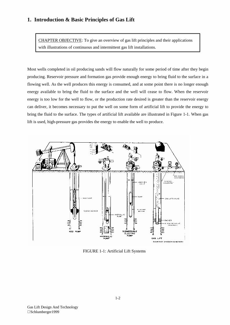
Most wells completed in oil producing sands will flow naturally for some period of time after they begin
producing. Reservoir pressure and formation gas provide enough energy to bring fluid to the surface in a
flowing well. As the well produces this energy is consumed, and at some point there is no longer enough
energy available to bring the fluid to the surface and the well will cease to flow. When the reservoir
energy is too low for the well to flow, or the production rate desired is greater than the reservoir energy
can deliver, it becomes necessary to put the well on some form of artificial lift to provide the energy to
bring the fluid to the surface. The types of artificial lift available are illustrated in Figure 1-1. When gas
lift is used, high-pressure gas provides the energy to enable the well to produce.
FIGURE 1-1: Artificial Lift Systems
1-3
Gas Lift Design And Technology Schlumberger1999
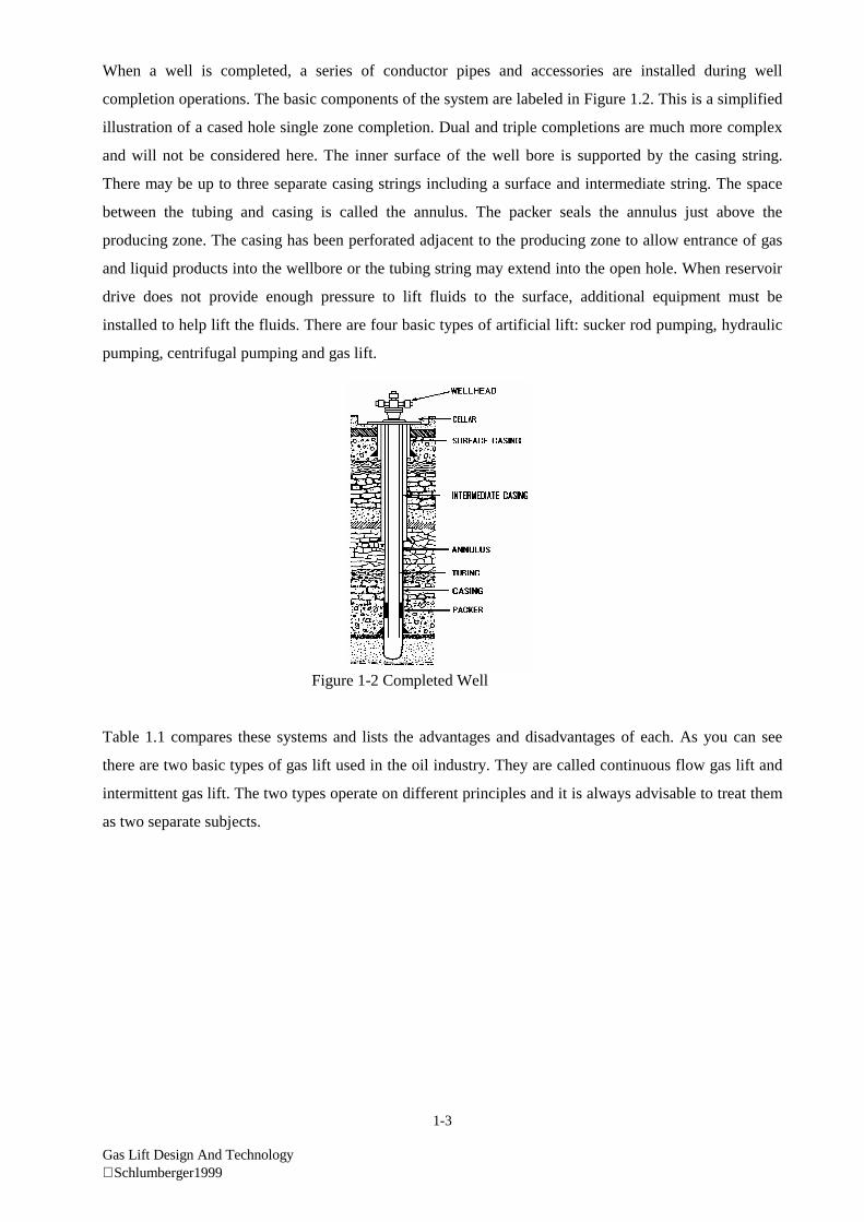
When a well is completed, a series of conductor pipes and accessories are installed during well
completion operations. The basic components of the system are labeled in Figure 1.2. This is a simplified
illustration of a cased hole single zone completion. Dual and triple completions are much more complex
and will not be considered here. The inner surface of the well bore is supported by the casing string.
There may be up to three separate casing strings including a surface and intermediate string. The space
between the tubing and casing is called the annulus. The packer seals the annulus just above the
producing zone. The casing has been perforated adjacent to the producing zone to allow entrance of gas
and liquid products into the wellbore or the tubing string may extend into the open hole. When reservoir
drive does not provide enough pressure to lift fluids to the surface, additional equipment must be
installed to help lift the fluids. There are four basic types of artificial lift: sucker rod pumping, hydraulic
pumping, centrifugal pumping and gas lift.
Figure 1-2 Completed Well
Table 1.1 compares these systems and lists the advantages and disadvantages of each. As you can see
there are two basic types of gas lift used in the oil industry. They are called continuous flow gas lift and
intermittent gas lift. The two types operate on different principles and it is always advisable to treat them
as two separate subjects.
1-4
Gas Lift Design And Technology Schlumberger1999
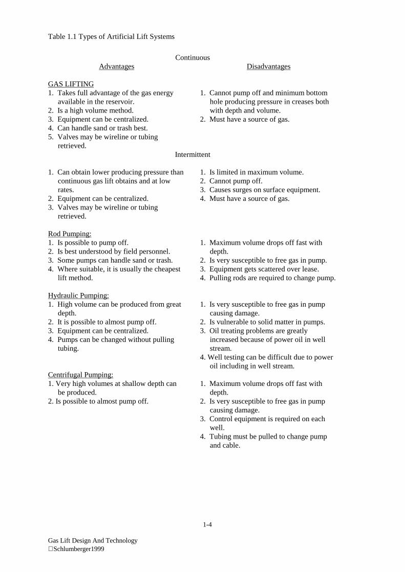
Table 1.1 Types of Artificial Lift Systems
ContinuousAdvantages
GAS LIFTING1. Takes full advantage of the gas energy
available in the reservoir.2. Is a high volume method.3. Equipment can be centralized.4. Can handle sand or trash best.5. Valves may be wireline or tubing
retrieved.
Disadvantages
1. Cannot pump off and minimum bottomhole producing pressure in creases bothwith depth and volume.
2. Must have a source of gas.
Intermittent
1. Can obtain lower producing pressure thancontinuous gas lift obtains and at lowrates.
2. Equipment can be centralized.3. Valves may be wireline or tubing
retrieved.
Rod Pumping:1. Is possible to pump off.2. Is best understood by field personnel.3. Some pumps can handle sand or trash.4. Where suitable, it is usually the cheapest
lift method.
Hydraulic Pumping:1. High volume can be produced from great
depth.2. It is possible to almost pump off.3. Equipment can be centralized.4. Pumps can be changed without pulling
tubing.
Centrifugal Pumping:1. Very high volumes at shallow depth can
be produced.2. Is possible to almost pump off.
1. Is limited in maximum volume.2. Cannot pump off.3. Causes surges on surface equipment.4. Must have a source of gas.
1. Maximum volume drops off fast withdepth.
2. Is very susceptible to free gas in pump.3. Equipment gets scattered over lease.4. Pulling rods are required to change pump.
1. Is very susceptible to free gas in pumpcausing damage.
2. Is vulnerable to solid matter in pumps.3. Oil treating problems are greatly
increased because of power oil in wellstream.
4. Well testing can be difficult due to poweroil including in well stream.
1. Maximum volume drops off fast withdepth.
2. Is very susceptible to free gas in pumpcausing damage.
3. Control equipment is required on eachwell.
4. Tubing must be pulled to change pumpand cable.
1-5
Gas Lift Design And Technology Schlumberger1999
Advantages and Limitations of Gas Lift
The flexibility of gas lift in terms of production rates and required depth of lift cannot be matched by
other methods of artificial lift for most wells if adequate injection gas pressure and volume are available.
Gas lift is considered one of the most forgiving forms of artificial lift since a poorly designed installation
will normally gas lift some fluid. Many efficient gas lift installations with wireline retrievable gas lift
valve mandrels are designed with minimal well information for locating the mandrel depths upon initial
well completion in offshore and inaccessible onshore locations.
Highly deviated wells that produce sand and have a high formation/liquid ratio are excellent candidates
for gas lift when artificial lift is needed. Many gas lift installations are designed to increase the daily
production from flowing wells. No other method is as ideally suited for through-flow-line (TFL) ocean
floor completions as a gas lift system. Maximum production is possible by gas lift from a well with
small casing and with high deliverability and bottomhole pressure.
Wireline retrievable gas lift valves can be replaced without killing a well with a load fluid or pulling the
tubing. Most gas lift valves are simple devices with few moving parts. Sand laden well production fluids
do not pass through the operating gas lift valve. The subsurface gas lift equipment is relatively
inexpensive. The surface injection gas control equipment is simple and light in weight. This surface
equipment requires little maintenance and practically no space for installation. The reported overall
reliability, replacement and operating costs for subsurface gas lift equipment are lower than for other
methods of lift.
The most important limitation of gas lift operation is the lack of formation gas or the availability of an
outside source of gas. Other limitations include wide well spacing and unavailable space for
compressors on offshore platforms. Gas lift is seldom applicable to single well installation and to widely
spaced wells that are not suited for a centrally located power system. Gas lift is not recommended for
lifting viscous crude, a super-saturated brine or an emulsion. Old casing, dangerously sour gas and long
small ID flowlines can eliminate gas lift operations. Wet gas without proper dehydration will reduce the
reliability of gas lift operations.
Designing systems of artificial lift requires obtaining considerable information about well conditions.
Although some measurements are taken, some of the required data must be estimated by making certain
inferences from available data. A system of nomenclature has been adapted by petroleum experts to
designate certain well data.
1-6
Gas Lift Design And Technology Schlumberger1999
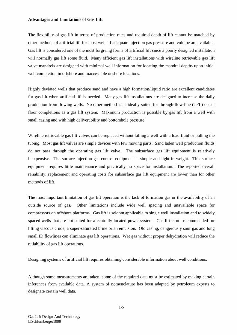
It is important to know the pressure at various points in the system. Pressure is expressed in pounds per
square inch (psi) or [Kilopascals (kPa)]. For gas lift calculations, pressure is understood as gauge
pressure (psig).
Figure 1.3 illustrates some points in a well where pressure readings are taken. Pressure at the bottom ofthe hole (Pbh) caused by the drive mechanism within the reservoir can be expressed as a static pressure
(Pbhs) or if the well is flowing as a flowing bottom hole pressure (Pbhf). If a flowing well is shut in, the
bottom hole pressure is expressed as Pws. It is necessary to use pressure data along the tubing string (Pt)
and within the tubing casing annulus (Pc). The tubing pressure at the wellhead is referred to as Pwh.
Temperature is measured along the tubing string from the wellhead (Twh) to bottom hole (Tbh) as can be
seen in Figure 1.4. Temperature is usually expressed in degrees Fahrenheit or degrees Celsius.
Figure 1.3 Figure 1.4
Well Measurements Well Temperature Measurements
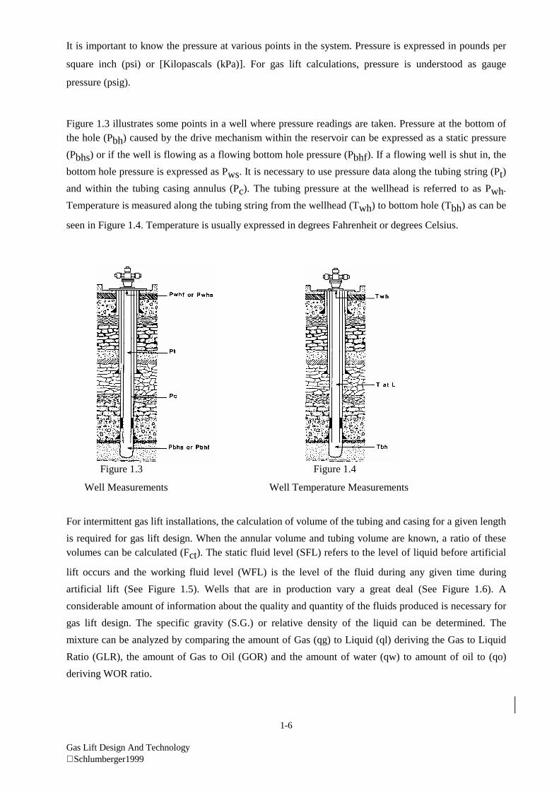
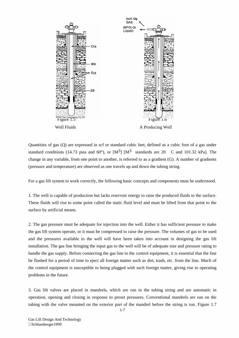
For intermittent gas lift installations, the calculation of volume of the tubing and casing for a given length
is required for gas lift design. When the annular volume and tubing volume are known, a ratio of thesevolumes can be calculated (Fct). The static fluid level (SFL) refers to the level of liquid before artificial
lift occurs and the working fluid level (WFL) is the level of the fluid during any given time during
artificial lift (See Figure 1.5). Wells that are in production vary a great deal (See Figure 1.6). A
considerable amount of information about the quality and quantity of the fluids produced is necessary for
gas lift design. The specific gravity (S.G.) or relative density of the liquid can be determined. The
mixture can be analyzed by comparing the amount of Gas (qg) to Liquid (ql) deriving the Gas to Liquid
Ratio (GLR), the amount of Gas to Oil (GOR) and the amount of water (qw) to amount of oil to (qo)
deriving WOR ratio.
1-7
Gas Lift Design And Technology Schlumberger1999
Figure 1.5 Figure 1.6
Well Fluids A Producing Well
Quantities of gas (Q) are expressed in scf or standard cubic feet, defined as a cubic foot of a gas under
standard conditions (14.73 psia and 60°), or [M3] [M3 standards are 20� C and 101.32 kPa]. The
change in any variable, from one point to another, is referred to as a gradient (G). A number of gradients
(pressure and temperature) are observed as one travels up and down the tubing string.
For a gas lift system to work correctly, the following basic concepts and components must be understood.
1. The well is capable of production but lacks reservoir energy to raise the produced fluids to the surface.
These fluids will rise to some point called the static fluid level and must be lifted from that point to the
surface by artificial means.
2. The gas pressure must be adequate for injection into the well. Either it has sufficient pressure to make
the gas lift system operate, or it must be compressed to raise the pressure. The volumes of gas to be used
and the pressures available to the well will have been taken into account in designing the gas lift
installation. The gas line bringing the input gas to the well will be of adequate size and pressure rating to
handle the gas supply. Before connecting the gas line to the control equipment, it is essential that the line
be flushed for a period of time to eject all foreign matter such as dirt, trash, etc. from the line. Much of
the control equipment is susceptible to being plugged with such foreign matter, giving rise to operating
problems in the future.
3. Gas lift valves are placed in mandrels, which are run in the tubing string and are automatic in
operation, opening and closing in response to preset pressures. Conventional mandrels are run on the
tubing with the valve mounted on the exterior part of the mandrel before the string is run. Figure 1.7
1-8
Gas Lift Design And Technology Schlumberger1999
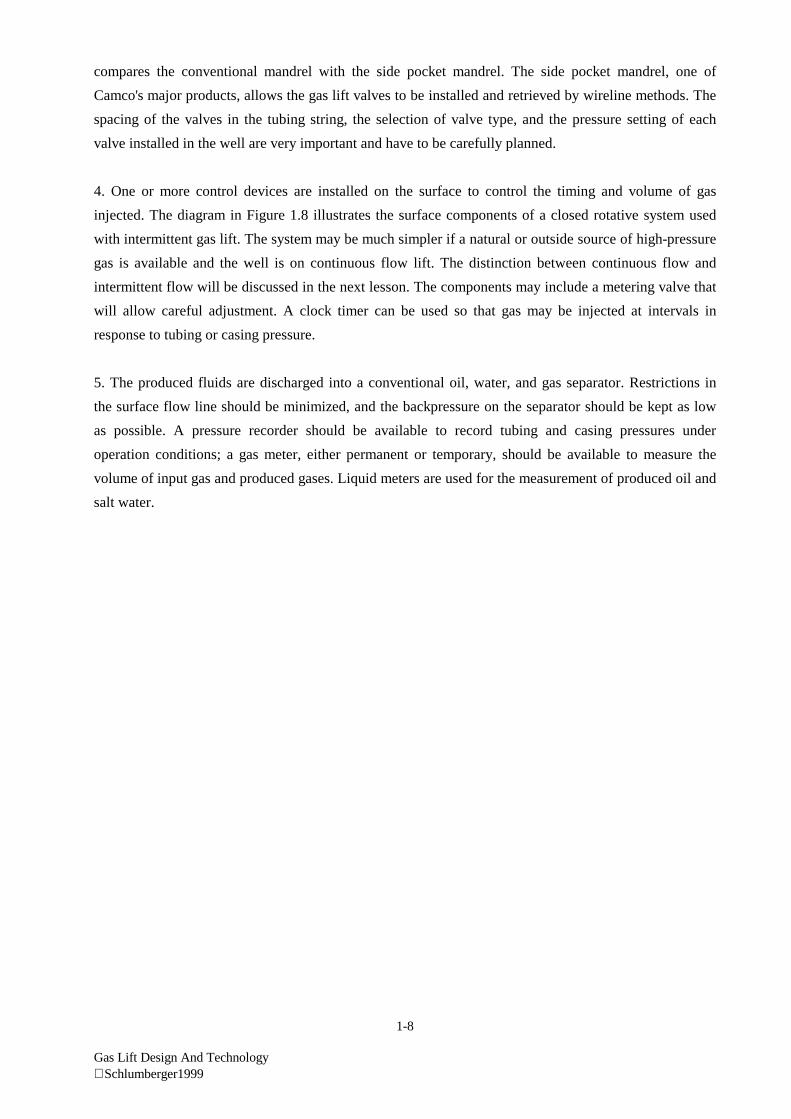
compares the conventional mandrel with the side pocket mandrel. The side pocket mandrel, one of
Camco's major products, allows the gas lift valves to be installed and retrieved by wireline methods. The
spacing of the valves in the tubing string, the selection of valve type, and the pressure setting of each
valve installed in the well are very important and have to be carefully planned.
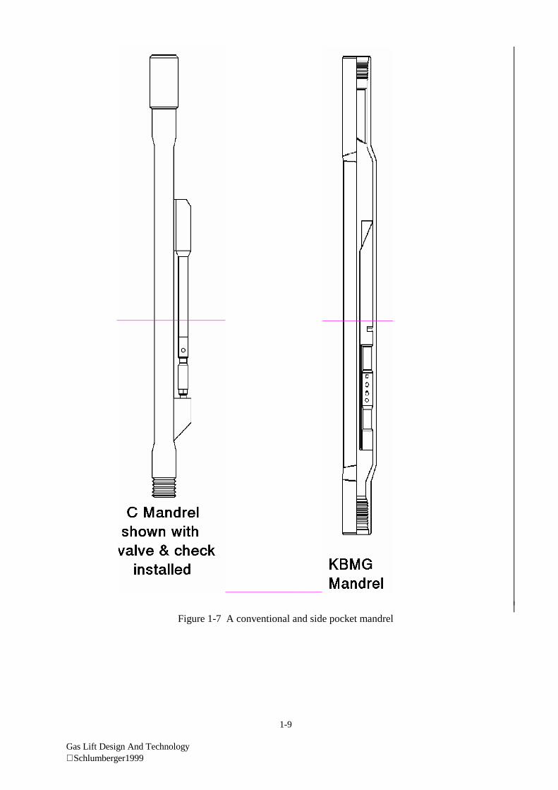
4. One or more control devices are installed on the surface to control the timing and volume of gas
injected. The diagram in Figure 1.8 illustrates the surface components of a closed rotative system used
with intermittent gas lift. The system may be much simpler if a natural or outside source of high-pressure
gas is available and the well is on continuous flow lift. The distinction between continuous flow and
intermittent flow will be discussed in the next lesson. The components may include a metering valve that
will allow careful adjustment. A clock timer can be used so that gas may be injected at intervals in
response to tubing or casing pressure.
5. The produced fluids are discharged into a conventional oil, water, and gas separator. Restrictions in
the surface flow line should be minimized, and the backpressure on the separator should be kept as low
as possible. A pressure recorder should be available to record tubing and casing pressures under
operation conditions; a gas meter, either permanent or temporary, should be available to measure the
volume of input gas and produced gases. Liquid meters are used for the measurement of produced oil and
salt water.
1-9
Gas Lift Design And Technology Schlumberger1999
Figure 1-7 A conventional and side pocket mandrel
1-10
Gas Lift Design And Technology Schlumberger1999
Figure 1.8 Surface Components of a Closed Rotative System with Intermittent Gas Lift
GAS LIFT VALVES:
A gas lift valve is designed to stay closed until certain conditions of pressure in the annulus and tubing
are met. When the valve opens, it permits gas or fluid to pass from the casing annulus into the tubing.
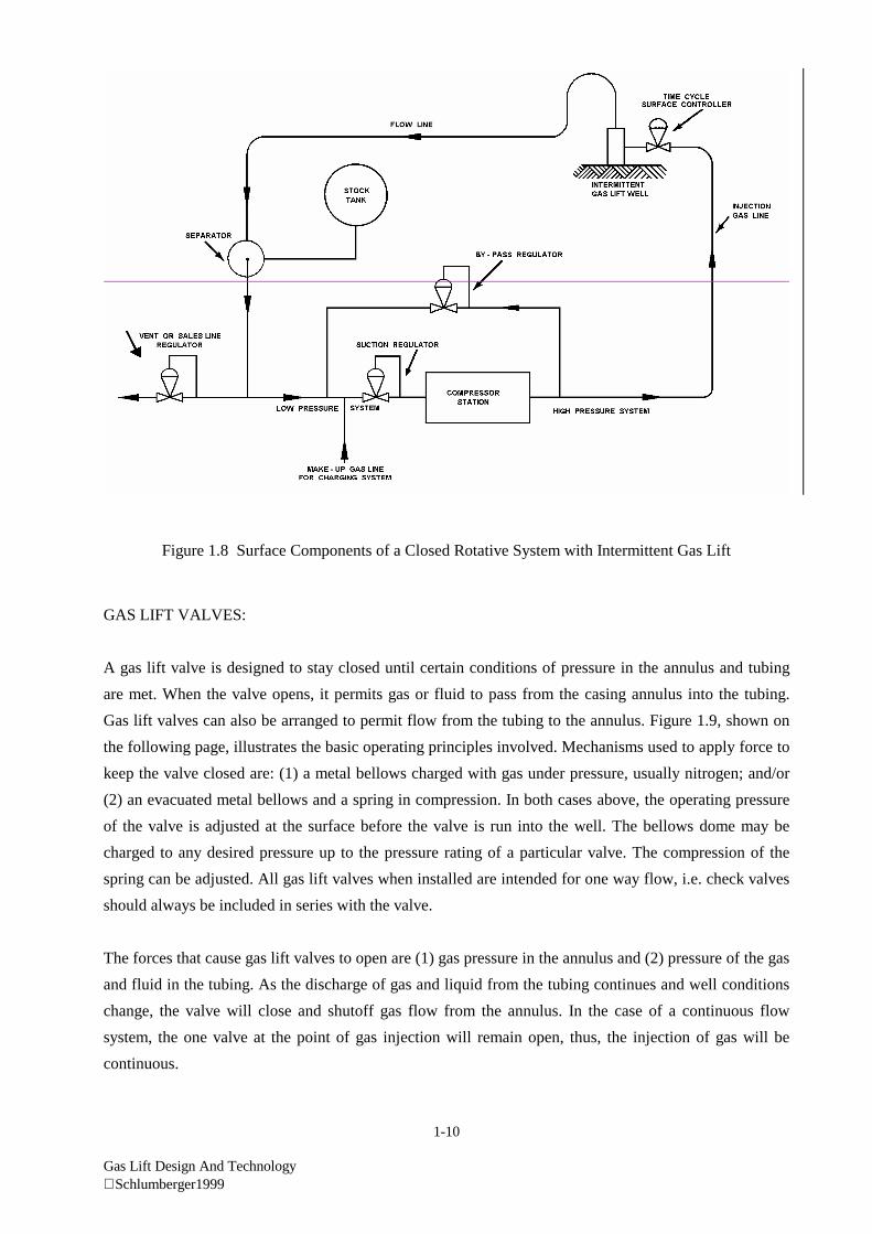
Gas lift valves can also be arranged to permit flow from the tubing to the annulus. Figure 1.9, shown on
the following page, illustrates the basic operating principles involved. Mechanisms used to apply force to
keep the valve closed are: (1) a metal bellows charged with gas under pressure, usually nitrogen; and/or
(2) an evacuated metal bellows and a spring in compression. In both cases above, the operating pressure
of the valve is adjusted at the surface before the valve is run into the well. The bellows dome may be
charged to any desired pressure up to the pressure rating of a particular valve. The compression of the
spring can be adjusted. All gas lift valves when installed are intended for one way flow, i.e. check valves
should always be included in series with the valve.
The forces that cause gas lift valves to open are (1) gas pressure in the annulus and (2) pressure of the gas
and fluid in the tubing. As the discharge of gas and liquid from the tubing continues and well conditions
change, the valve will close and shutoff gas flow from the annulus. In the case of a continuous flow
system, the one valve at the point of gas injection will remain open, thus, the injection of gas will be
continuous.
1-11
Gas Lift Design And Technology Schlumberger1999
In the case of intermittent flow, the injection valve opens and closes while the upper valves in the well
may open to assist lifting the slug to the surface. The gas injection valve, placed at the bottom of the fluid
column in the tubing, will open when pressure in the annulus reaches the required pressure and close
when pressure falls below that level.
Gas lift valves using pressure operation principles date back to the King Valve patented in 1944, and
numerous bellows operated valves have been developed since that date. A most significant contribution
to the industry was the invention of the Wireline Retrievable Valve in 1954.
An operating gas lift valve is installed to control the point of gas injection. Valves are installed above the
desired point of injection to unload the well. After unloading, they close to eliminate gas injection above
the operating valve.
For most continuous flow designs, the operating gas lift valve acts as a pressure regulator while the
surface choke provides for gas flow regulation.
Figure 1.9 Bellows type gas lift valve
1-12
Gas Lift Design And Technology Schlumberger1999
Applications of Gas Lift
Gas lifting of water with a small amount of oil used in the United States as early as 1846. Compressed air
is known to have been used earlier to lift water. In fact, it has been reported that compressed air was used
to lift water from wells in Germany as early as the eighteenth century. These early systems operated in a
very simple manner by the introduction of air down the tubing and up the casing. Aeration of the fluid in
the casing tubing annulus decreased the weight of the fluid column so that fluid would rise to the surface
and flow out of the well. The process was sometimes reversed by injecting down the casing and
producing through the tubing.
Air lift continued in use for lifting oil from wells by many operators, but it was not until the mid-1920's
that gas for lifting fluid became more widely available. Gas, being lighter than air, gave better
performance than air, lessened the hazards created by air when exposed to combustible materials and
decreased equipment deterioration caused by oxidation. During the 1930's, several types of gas lift valves
became available to the oil producing industry for gas lifting oil wells. Gas lift was soon accepted as a
competitive method of production, especially when gas at adequate pressures was available for lift
purposes. Two trends have developed in recent years:
1. A larger percentage of oil produced is from wells whose reservoir energy has been
depleted to the point that some form of artificial lift is required.
2. The commercial value of gas in many areas has multiplied many times; with the
increasing cost of gas, gas used to produce oil has achieved recognition as a hydrocarbon
of specific value. It should be remembered that gas is not consumed during gas lift. The
energy contained in the flowing gas is utilized but the net quantity remains the same.
Gas lift is a process of lifting fluids from a well by the continuous injection of high-pressure gas to
supplement the reservoir energy (continuous flow), or by injecting gas beneath an accumulated liquid
slug for a short time to move the slug to the surface (intermittent lift). The injected gas moves the fluid to
the surface by one or a combination of the following: reducing the fluid load pressure on the formation
because of decreased fluid density, expansion of injected gas, and displacing the fluid. In addition to
serving as a primary method of artificial lift, gas lift can also be used efficiently and effectively to
accomplish the following objectives:
1. To enable wells that will not flow naturally to produce.
2. To increase production rates in flowing wells.
3. To unload a well that will later flow naturally.
4. To remove or unload fluids from gas wells and to keep the gas well unloaded (usually intermittent , but
can be continuous).
1-13
Gas Lift Design And Technology Schlumberger1999
5. To backflow saltwater disposal wells to remove sands and other solids that can plug the perforations in
the well.
6. In water source (aquifer) wells to produce the large volumes of water necessary for water flood
applications.
Although other types of artificial lift may offer certain advantages, gas lift is suitable for almost every
type of well to be placed on artificial lift. An added advantage to gas lift is its versatility. Once an
installation is made, changes in design can be accomplished to reflect changes in well conditions. This is
particularly true when wireline retrievable valves are used.
It should be remembered that "natural flow" can be a form of gas lift. The energy of compressed gas in
the reservoir may be the principle force that raises the fluids to the surface. The energy of compressed
gas is utilized in two ways:
1. Pressure of the gas exerted against the oil at the bottom of the tubing is frequently sufficient to
lift the entire column of oil to the surface.
2. Aeration of the column of oil by gas bubbles entering it at the bottom of the tubing reduces the
density of the column of oil. As the gas moves up the tubing, gas expands because of the
reduction of pressure and the column of oil becomes even less dense.
With the density of the column thus reduced, less pressure is required from the reservoir to discharge the
oil to the surface. Natural flow in the well continues until a change of conditions causes it to cease
flowing. One change is the depletion of reservoir pressure until it no longer exerts sufficient force to
move the oil up the tubing. A second change is the increase of water percentage in the flow. When a well
"loads up" with water from the reservoir, more pressure is required to lift the column of fluid as water is
denser than oil. Also, the water does not contain gas in solution that would reduce the density of the
column.
The term gas lift covers a variety of practices by which gas is used to increase the production of a well or
to restore production where the well is dead. It may require a perforation or a jet collar in the tubing
string, or the more complex devices, gas lift valves, which are manufactured to meet specific operating
conditions and placed in the well according to carefully developed formulas. Gas lift may operate
continuously or intermittently. It may be installed in a well at any depth from a few hundred feet [100
meters] to twelve thousand feet [3700 meters] or more.
The basic principles of natural flow and gas lift are essentially the same, i.e. density of the column is
reduced and pressure raises the fluid to the surface. In a gas lift well, the gas is introduced from external
sources under controlled conditions through gas lift valves installed for that purpose.
1-14
Gas Lift Design And Technology Schlumberger1999
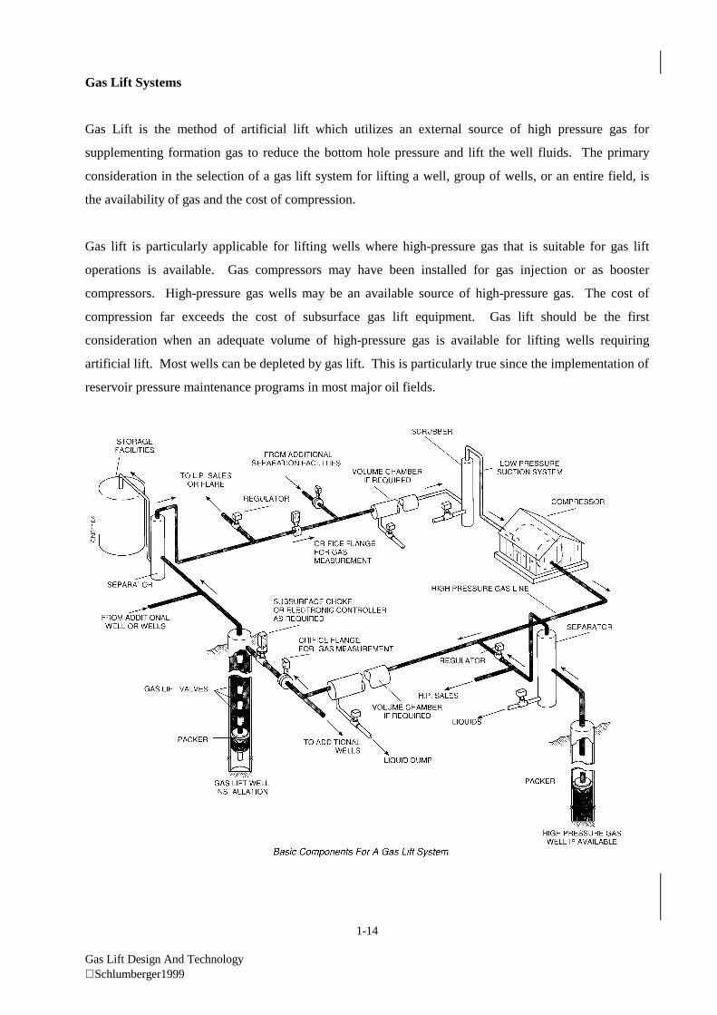
Gas Lift Systems
Gas Lift is the method of artificial lift which utilizes an external source of high pressure gas for
supplementing formation gas to reduce the bottom hole pressure and lift the well fluids. The primary
consideration in the selection of a gas lift system for lifting a well, group of wells, or an entire field, is
the availability of gas and the cost of compression.
Gas lift is particularly applicable for lifting wells where high-pressure gas that is suitable for gas lift
operations is available. Gas compressors may have been installed for gas injection or as booster
compressors. High-pressure gas wells may be an available source of high-pressure gas. The cost of
compression far exceeds the cost of subsurface gas lift equipment. Gas lift should be the first
consideration when an adequate volume of high-pressure gas is available for lifting wells requiring
artificial lift. Most wells can be depleted by gas lift. This is particularly true since the implementation of
reservoir pressure maintenance programs in most major oil fields.
1-15
Gas Lift Design And Technology Schlumberger1999
Closed Rotative Gas Lift System
Most gas lift systems are designed to recirculate the lift gas. The low-pressure gas from the production
separator is piped to the suction of the compressor station. The high-pressure gas from the discharge of
the compressor station is injected into the well to lift the fluids from the well. Excess gas production
may be sold, injected into a formation or vented to the atmosphere. This closed loop for the gas is
referred to as a closed rotative system. Continuous flow gas lift operations are preferable with a closed
rotative system because of the constant injection gas requirement and constant return of the gas to the
low pressure facilities. Intermittent gas lift operations are particularly difficult to regulate and operate
efficiently in small closed rotative systems with limited gas storage capacities in the low and high
pressure gas lines and surface facilities.
CONTINUOUS FLOW GAS LIFT
The principle underlying the continuous flow gas lift method is that energy resulting from expansion of
gas from a high pressure to a lower pressure is utilized in promoting the flow of well fluids in a vertical
tube or annular configurations. Utilization of this gas energy is accomplished by the continuous injection
of a controlled stream of gas into a rising stream of well fluids in such a manner that useful work is
performed in lifting the well fluids.
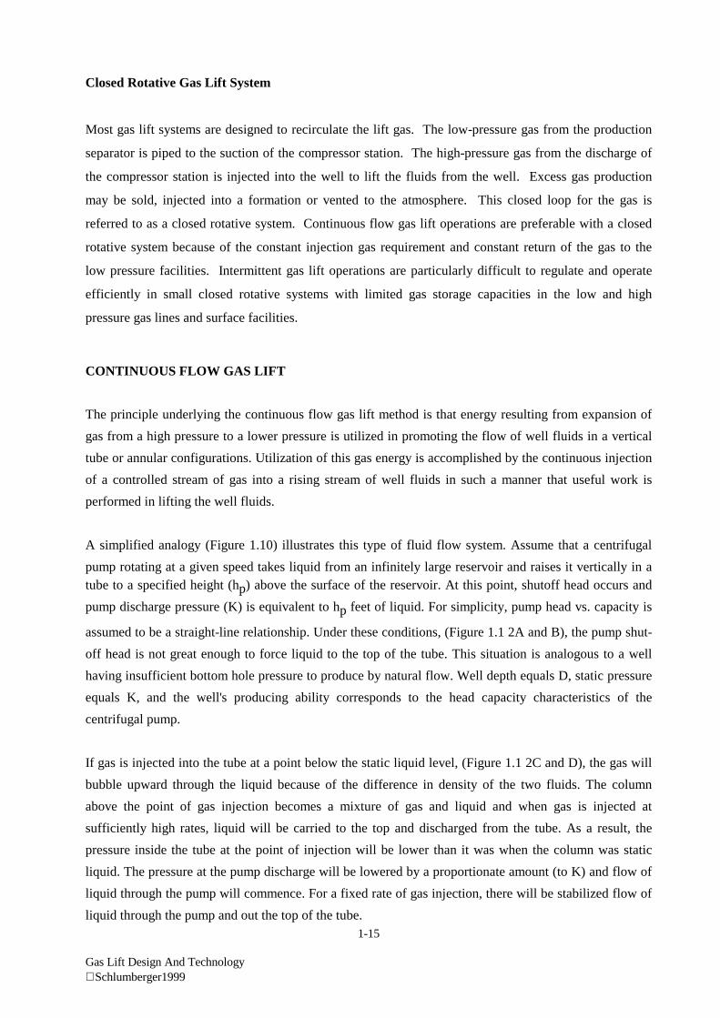
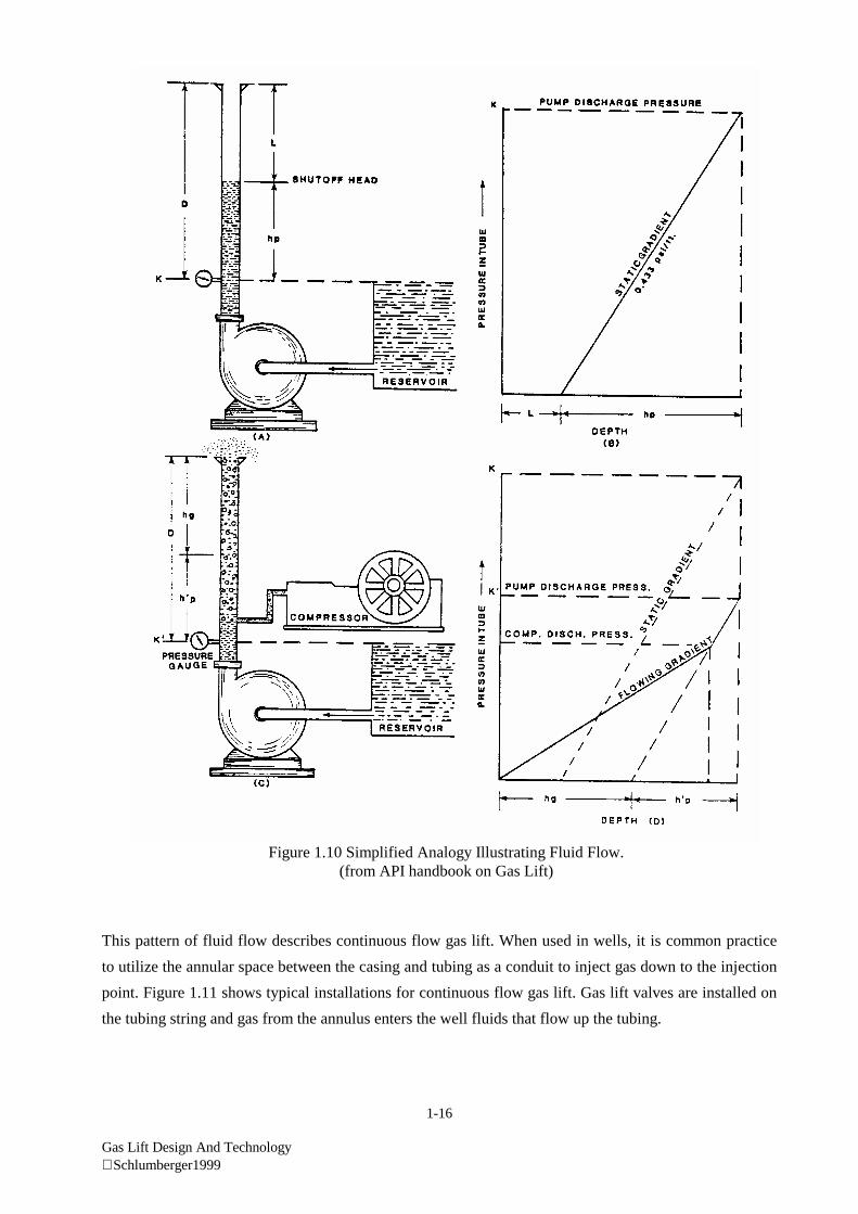
A simplified analogy (Figure 1.10) illustrates this type of fluid flow system. Assume that a centrifugal
pump rotating at a given speed takes liquid from an infinitely large reservoir and raises it vertically in atube to a specified height (hp) above the surface of the reservoir. At this point, shutoff head occurs and
pump discharge pressure (K) is equivalent to hp feet of liquid. For simplicity, pump head vs. capacity is
assumed to be a straight-line relationship. Under these conditions, (Figure 1.1 2A and B), the pump shut-
off head is not great enough to force liquid to the top of the tube. This situation is analogous to a well
having insufficient bottom hole pressure to produce by natural flow. Well depth equals D, static pressure
equals K, and the well's producing ability corresponds to the head capacity characteristics of the
centrifugal pump.
If gas is injected into the tube at a point below the static liquid level, (Figure 1.1 2C and D), the gas will
bubble upward through the liquid because of the difference in density of the two fluids. The column
above the point of gas injection becomes a mixture of gas and liquid and when gas is injected at
sufficiently high rates, liquid will be carried to the top and discharged from the tube. As a result, the
pressure inside the tube at the point of injection will be lower than it was when the column was static
liquid. The pressure at the pump discharge will be lowered by a proportionate amount (to K) and flow of
liquid through the pump will commence. For a fixed rate of gas injection, there will be stabilized flow of
liquid through the pump and out the top of the tube.
1-16
Gas Lift Design And Technology Schlumberger1999
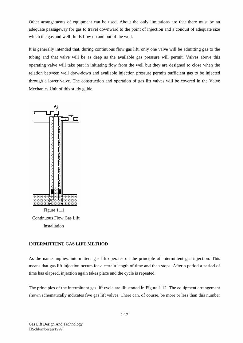
This pattern of fluid flow describes continuous flow gas lift. When used in wells, it is common practice
to utilize the annular space between the casing and tubing as a conduit to inject gas down to the injection
point. Figure 1.11 shows typical installations for continuous flow gas lift. Gas lift valves are installed on
the tubing string and gas from the annulus enters the well fluids that flow up the tubing.
Figure 1.10 Simplified Analogy Illustrating Fluid Flow.(from API handbook on Gas Lift)
1-17
Gas Lift Design And Technology Schlumberger1999
Other arrangements of equipment can be used. About the only limitations are that there must be an
adequate passageway for gas to travel downward to the point of injection and a conduit of adequate size
which the gas and well fluids flow up and out of the well.
It is generally intended that, during continuous flow gas lift, only one valve will be admitting gas to the
tubing and that valve will be as deep as the available gas pressure will permit. Valves above this
operating valve will take part in initiating flow from the well but they are designed to close when the
relation between well draw-down and available injection pressure permits sufficient gas to be injected
through a lower valve. The construction and operation of gas lift valves will be covered in the Valve
Mechanics Unit of this study guide.
Figure 1.11
Continuous Flow Gas Lift
Installation
INTERMITTENT GAS LIFT METHOD
As the name implies, intermittent gas lift operates on the principle of intermittent gas injection. This
means that gas lift injection occurs for a certain length of time and then stops. After a period a period of
time has elapsed, injection again takes place and the cycle is repeated.
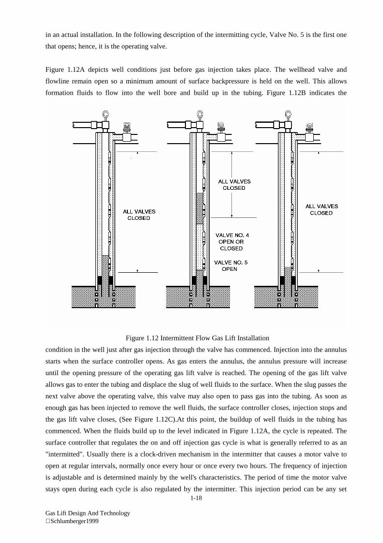
The principles of the intermittent gas lift cycle are illustrated in Figure 1.12. The equipment arrangement
shown schematically indicates five gas lift valves. There can, of course, be more or less than this number
1-18
Gas Lift Design And Technology Schlumberger1999
in an actual installation. In the following description of the intermitting cycle, Valve No. 5 is the first one
that opens; hence, it is the operating valve.
Figure 1.12A depicts well conditions just before gas injection takes place. The wellhead valve and
flowline remain open so a minimum amount of surface backpressure is held on the well. This allows
formation fluids to flow into the well bore and build up in the tubing. Figure 1.12B indicates the
condition in the well just after gas injection through the valve has commenced. Injection into the annulus
starts when the surface controller opens. As gas enters the annulus, the annulus pressure will increase
until the opening pressure of the operating gas lift valve is reached. The opening of the gas lift valve
allows gas to enter the tubing and displace the slug of well fluids to the surface. When the slug passes the
next valve above the operating valve, this valve may also open to pass gas into the tubing. As soon as
enough gas has been injected to remove the well fluids, the surface controller closes, injection stops and
the gas lift valve closes, (See Figure 1.12C).At this point, the buildup of well fluids in the tubing has
commenced. When the fluids build up to the level indicated in Figure 1.12A, the cycle is repeated. The
surface controller that regulates the on and off injection gas cycle is what is generally referred to as an
"intermitted". Usually there is a clock-driven mechanism in the intermitter that causes a motor valve to
open at regular intervals, normally once every hour or once every two hours. The frequency of injection
is adjustable and is determined mainly by the well's characteristics. The period of time the motor valve
stays open during each cycle is also regulated by the intermitter. This injection period can be any set
Figure 1.12 Intermittent Flow Gas Lift Installation
1-19
Gas Lift Design And Technology Schlumberger1999
time, such as two minutes. It is also possible to regulate the injection period with a tubing or casing
pressure shutoff. In this case, the intermitter shuts off injection gas whenever the tubing or casing
pressure increases to some preset value. Intermittent gas lift is usually applied to wells having low
productivity indexes that generally result in relatively low producing rates. A low productivity index
means that the buildup of well fluids in the bottom of the well will take place over a fairly long period of
time.
Open and Closed Gas Lift Installations
Most tubing flow gas lift installations will include a packer to stabilize the fluid level in the casing
annulus after a well has unloaded. A packer is installed in a low flowing bottomhole pressure well to
prevent injection gas from blowing around the lower end of the tubing. A closed gas lift installation
implies that there is a packer and a standing valve in the well. An installation without a standing valve is
referred to as semi-closed, which is widely used for continuous flow operations. An installation without
a packer or standing valve is an open installation. An open installation is seldom recommended unless
the well has a flowing bottomhole pressure that significantly exceeds the injection gas pressure and
packer removal may be difficult or impossible because of sand, scale, etc. Casing flow gas lift requires
an open installation since the production conduit is the casing annulus. A packer is required for gas
lifting low bottomhole pressure wells to isolate the injection gas in the casing annulus and allow surface
control of the injection gas volumetric rate to the well. Most intermittent gas lift installations will
include a packer and possibly a standing valve. Although illustrations of nearly all-intermittent gas lift
installations show a standing valve, many actual installations do not include this valve. If the
permeability of the well is very low, a standing valve may not be needed.
The advantages of a packer are particularly important for gas lift installations where the injection gas line
pressure varies or the injection gas supply is periodically interrupted. If the installation does not include
a packer, most wells must be unloaded or partially unloaded after each extended shutdown. More
damage to gas lift valves can occur during unloading operations than any time in the life of a gas lift
installation. If the injection gas line pressure varies, the working fluid level changes in an open
installation. The result is a liquid washing action through all of the valves below the working fluid level.
This continuing fluid transfer can eventually fluid-cut the seat assemblies of these lower gas lift valves.
A packer stabilizes the working fluid level, thus eliminating the need for unloading after a shutdown and
the fluid washing action from a varying injection gas line pressure.
1-20
Gas Lift Design And Technology Schlumberger1999
Considerations for Gas Lift Design and Operations
If a well can be gas lifted by continuous flow, this form of gas lift should be used to ensure a constant
injection gas circulation rate within the closed loop of a rotative gas lift system. Continuous flow
reduces the probability of pressure surges in the flowing bottomhole pressure, flowline and the low and
high pressure surface facilities that occur with intermittent gas lift operations. Over-design rather than
under-design of the gas lift valve spacing is always recommended when the well data are questionable.
The subsurface gas lift equipment in the well is the least expensive portion of a closed rotative gas lift
system. The larger OD gas lift valves are recommended for lifting high rate wells. The superior
injection gas volumetric throughput performance of the 1-1/2 inch OD gas lift valve as compared to the
1-inch OD valve is an important consideration for gas lift installations requiring a high injection gas
volumetric rate into the production conduit.
Most gas lift installation designs include several safety factors to compensate for errors in well
information and to allow for an increase in the injection gas pressure to open (adequately stroke) the
unloading and operating gas lift valves. It is difficult to properly design or analyze a gas lift installation
without understanding the operating characteristics of the gas lift valves in a well. The operators should
be familiar with the construction and operating principles of the gas lift valves in their wells. When an
installation is properly designed, all gas lift valves above an operating valve will be closed and all valves
below will be open in a continuous flow installation.
A large bore seating nipple which is designed to receive a lock is recommended near the lower end of the
tubing for many gas lift installations. There are numerous applications for a seating nipple which include
installation of a standing valve for testing the tubing and the gas lift valve checks. A standing valve may
be needed in an intermittent gas lift installation. A wireline lock provides the means to secure and pack-
off a bottomhole pressure gauge for conducting pressure transient tests, etc. The lock assembly should
have an equalizing valve if the tubing will be blanked-off. The pressure across the lock can be equalized
before the lock is disengaged from the nipple to prevent the wireline tool string from being blown up the
hole.
Continuous Flow Unloading Sequence
After a well is completed or worked over, the fluid level in the casing and tubing is usually at or near the
surface. The gas lift pressure available to unload the well is generally not sufficient to unload fluid to the
desired depth for gas injection. This is because the pressure caused by the static column of fluid in the
well at the desired depth of injection is greater than the available gas pressure at the depth of injection. In
1-21
Gas Lift Design And Technology Schlumberger1999
this case a series of unloading gas lift valves are installed in the well. These valves are designed to use
the available gas injection pressure to unload the well until the desired depth of injection is achieved.
Figure 1-13 through 1-20 detail the unloading sequence in a continuous flow gas lift well.
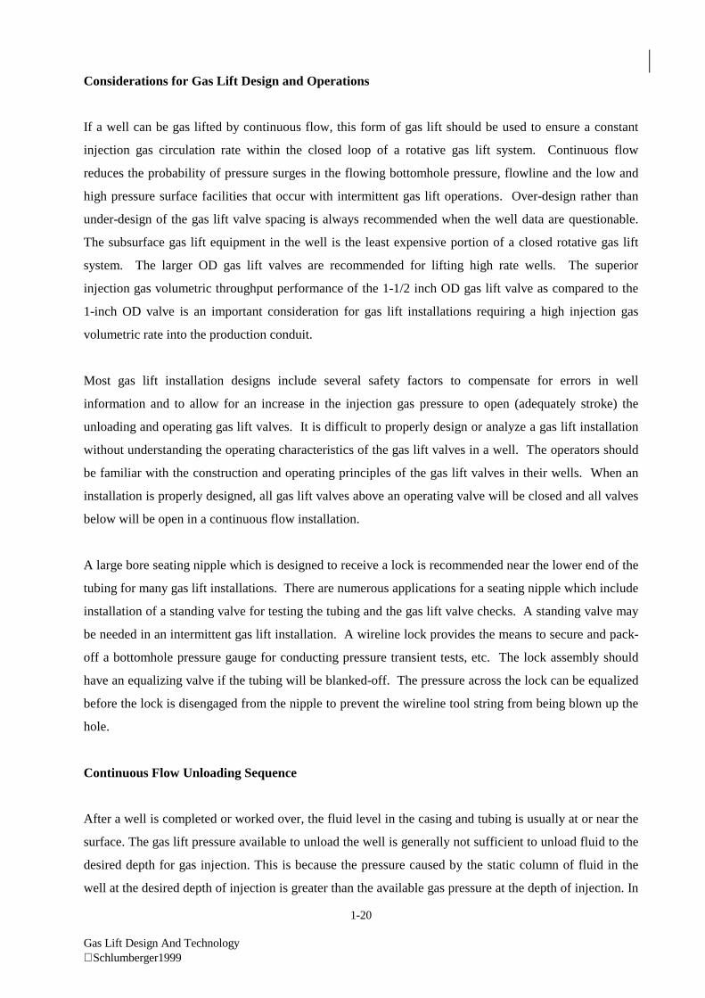
FIGURE 1-13
The fluid level in the casing and the tubing is at surface. No gas is being injected into the casing and no fluid is being produced. All the gas lift valves are open. Thepressure to open the valves is provided by the weight of the fluid in the casing and tubing.
Note that the fluid level in the tubing and casing will be determined by the shut in bottom hole pressure (SIBHP) and the hydrostatic head or weight of the column offluid which is in turn determined by the density. Water has a greater density than oil and thus the fluid level of a column of water will be lower than that of oil.
IN JE C T IO N G ASC H O K E C L O S E D
T O S E P AR A T O R /S T O C K T A NK
TOP VALVE OPEN
SECOND VALVEOPEN
THIRD VALVEOPEN
FOURTH VALVEOPEN
0
2000
6000
8000
10000
12000
14000
4000
2000 4000
PRESSURE PSI
DE
PT
H F
TT
VD
SIBHPTUBING PRESSURE
CASING PRESSURE
30001000 5000
CASING PRESSURE
TUBING PRESSURE
6000 7000
FIGURE 1-14
Gas injection into the casing has begun. Fluid is U-tubed through all the open gas lift valves. No formation fluids are being produced because the pressure in thewellbore at perforation depth is greater than the reservoir pressure i.e. no drawdown. All fluid produced is from the casing and the tubing. All fluid unloaded fromthe casing passes through the open gas lift valves. Because of this, it is important that the well be unloaded at a reasonable rate to prevent damage to the gas liftvalves.
IN JE C T IO N G ASC H O K E O P E N
T O S E P AR A T O R /S T O C K T A NK
TOP VALVE OPEN
SECOND VALVEOPEN
THIRD VALVEOPEN
FOURTH VALVEOPEN
0
2000
6000
8000
10000
12000
14000
4000
2000 4000
PRESSURE PSI
DE
PT
H F
TT
VD
SIBHPTUBING PRESSURE
CASING PRESSURE
30001000 5000 6000 7000
1-22
Gas Lift Design And Technology Schlumberger1999
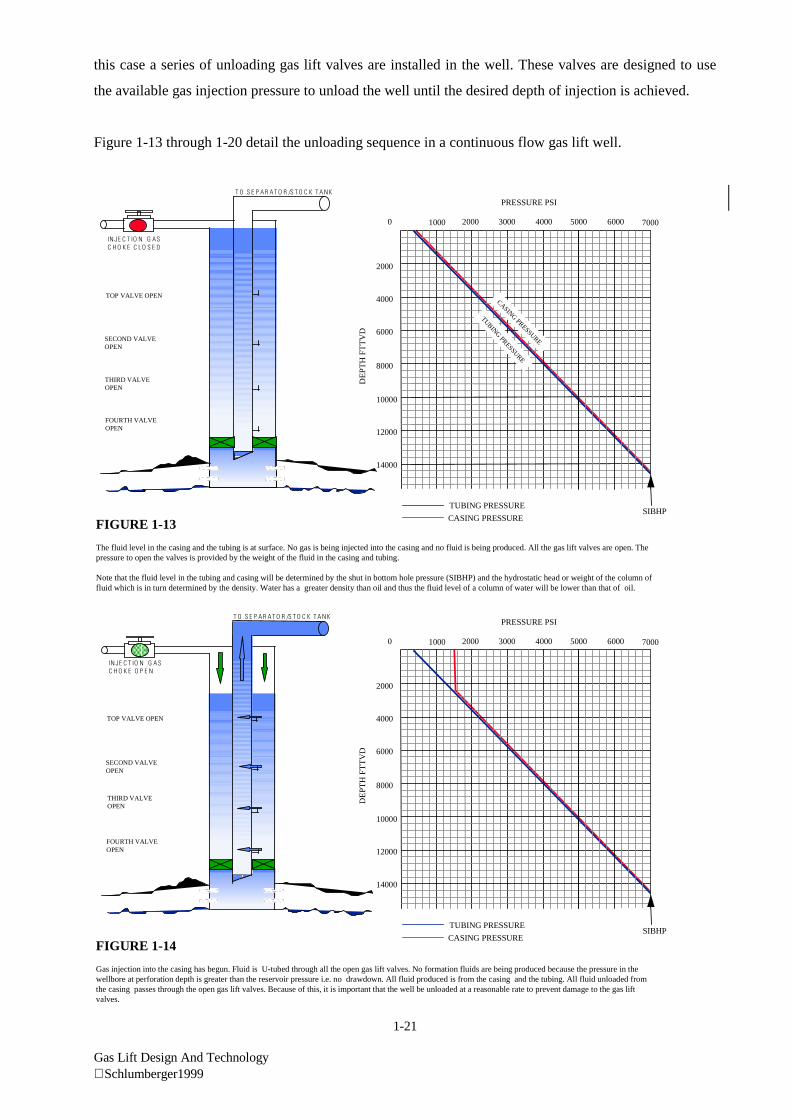
FIGURE 1-15
The fluid level has been unloaded to the top gas lift valve. This aerates the fluid above the top gas lift valve, decreasing the fluid density. This reduces the pressure inthe tubing at the top gas lift valve, and also reduces pressure in the tubing at all valves below the top valve. This pressure reduction allows casing fluid below the topgas lift valve to be U-tubed further down the well and unloaded through valves 2, 3 and 4.
If this reduction in pressure is sufficient to give some drawdown at the perforations then the well will start to produce formation fluid.
IN JE C T IO N G ASC H O K E O P E N
T O S E P AR A T O R /S T O C K T A NK
TOP VALVE OPEN
SECOND VALVEOPEN
THIRD VALVEOPEN
FOURTH VALVEOPEN
0
2000
6000
8000
10000
12000
14000
4000
2000 4000
PRESSURE PSI
DE
PT
H F
TT
VD
SIBHPTUBING PRESSURE
CASING PRESSURE
30001000 5000 6000 7000
FIGURE 1-16
The fluid level in the annulus has now been unloaded to just above valve number two. This has been posssible due to the increasing volume of gas passing throughnumber one reducing the pressure in the tubing at valve two thus enabling the U-tubing process to continue.
INJE C T IO N G ASC H O K E O P E N
T O S E P A R A T O R /S T O C K T A NK
TOP VALVE OPEN
SECOND VALVEOPEN
THIRD VALVEOPEN
FOURTH VALVEOPEN
0
2000
6000
8000
10000
12000
14000
4000
2000 4000
PRESSURE PSI
DE
PT
H F
TT
VD
SIBHPTUBING PRESSURE
CASING PRESSURE
30001000 5000
DRAWDOWN
6000 7000
FBHP
1-23
Gas Lift Design And Technology Schlumberger1999
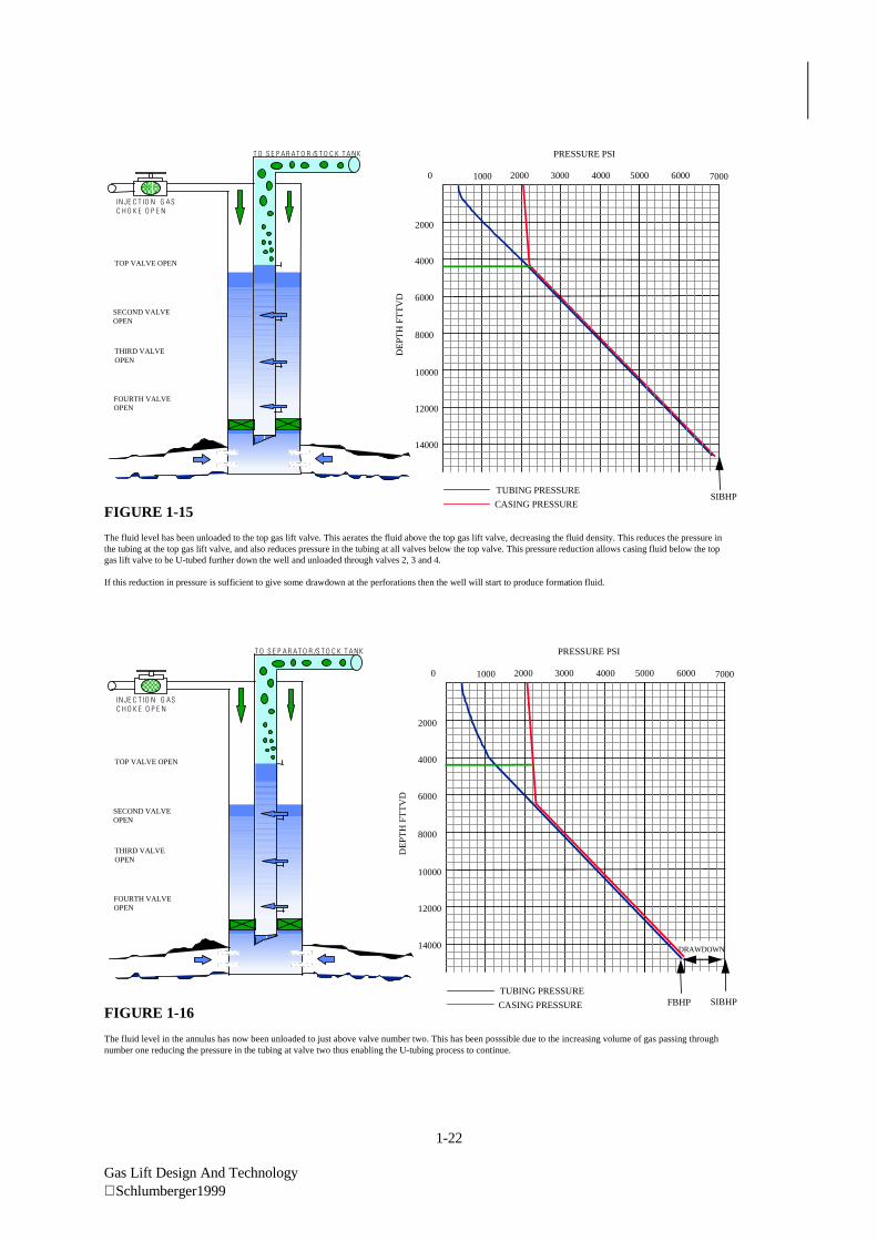
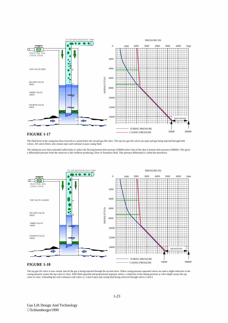
FIGURE 1-17
The fluid level in the casing has been lowered to a point below the second gas lift valve. The top two gas lift valves are open and gas being injected through bothvalves. All valves below also remain open and continue to pass casing fluid.
The tubing has now been unloaded sufficiently to reduce the flowing bottom hole pressure (FBHP) below that of the shut in bottom hole pressure (SIBHP). This givesa differential pressure from the reservoir to the wellbore producing a flow of formation fluid. This pressure differential is called the drawdown
INJE C T IO N G ASC H O K E O P E N
T O S E P A R A T O R /S T O C K T A NK
TOP VALVE OPEN
SECOND VALVEOPEN
THIRD VALVEOPEN
FOURTH VALVEOPEN
0
2000
6000
8000
10000
12000
14000
4000
2000 4000
PRESSURE PSI
DE
PT
H F
TT
VD
TUBING PRESSURE
CASING PRESSURE
30001000 5000
DRAWDOWN
6000 7000
FBHP SIBHP
FIGURE 1-18
The top gas lift valve is now closed, and all the gas is being injected through the second valve. When casing pressure operated valves are used a slight reduction in thecasing pressure causes the top valve to close. With fluid operated and proportional response valves, a reduction in the tubing pressure at valve depth causes the topvalve to close. Unloading the well continues with valves 2, 3 and 4 open and casing fluid being removed through valves 3 and 4.
INJE C T IO N G ASC H O K E O P E N
T O S E P A R A T O R /S T O C K T A NK
TOP VALVE CLOSED
SECOND VALVEOPEN
THIRD VALVEOPEN
FOURTH VALVEOPEN
0
2000
6000
8000
10000
12000
14000
4000
2000 4000
PRESSURE PSI
DE
PT
H F
TT
VD
TUBING PRESSURE
CASING PRESSURE
30001000 5000
DRAWDOWN
6000 7000
FBHP SIBHP
1-24
Gas Lift Design And Technology Schlumberger1999
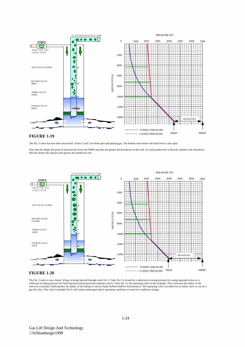
FIGURE 1-19
The No. 3 valve has now been uncovered. Valves 2 and 3 are both open and passing gas. The bottom valve below the fluid level is also open.
Note that the deeper the point of injection the lower the FBHP and thus the greater the drawdown on the well. As well productivity is directly related to the drawdownthen the deeper the injection the greater the production rate.
INJE C T IO N G ASC H O K E O P E N
T O S E P A R A T O R /S T O C K T A NK
TOP VALVE CLOSED
SECOND VALVEOPEN
THIRD VALVEOPEN
FOURTH VALVEOPEN
0
2000
6000
8000
10000
12000
14000
4000
2000 4000
PRESSURE PSI
DE
PT
H F
TT
VD
TUBING PRESSURE
CASING PRESSURE
30001000 5000
DRAWDOWN
6000 7000
FBHP SIBHP
FIGURE 1-20
The No. 2 valve is now closed. All gas is being injected through valve No 3. Valve No 2 is closed by a reduction in casing pressure for casing operated valves or areduction in tubing pressure for fluid operated and proportional response valves. Valve No 3 is the operating valve in this example. This is because the ability of thereservoir to produce fluid matches the ability of the tubing to remove fluids (Inflow/Outflow Performance). The operating valve can either be an orifice valve or can be agas lift valve. The valve in mandrel No 4 will remain submerged unless operating conditions or reservoir conditions change.
INJE C T IO N G A SC H O K E O P E N
T O S E P A R AT O R /S T O C K T A NK
TOP VALVE CLOSED
SECOND VALVECLOSED
THIRD VALVEOPEN
FOURTH VALVEOPEN
0
2000
6000
8000
10000
12000
14000
4000
2000 4000
PRESSURE PSI
DE
PT
H F
TT
VD
TUBING PRESSURE
CASING PRESSURE
30001000 5000
DRAWDOWN
6000 7000
FBHP SIBHP
1-25
Gas Lift Design And Technology Schlumberger1999
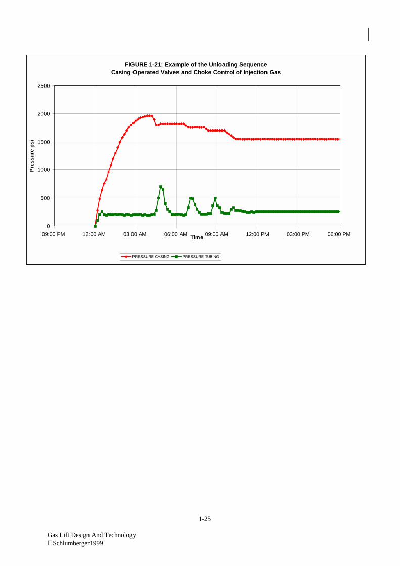
FIGURE 1-21: Example of the Unloading SequenceCasing Operated Valves and Choke Control of Injection Gas
0
500
1000
1500
2000
2500
09:00 PM 12:00 AM 03:00 AM 06:00 AM 09:00 AM 12:00 PM 03:00 PM 06:00 PMTime
Pre
ssu
re p
si
PRESSURE CASING PRESSURE TUBING
2-1
Gas Lift Design And Technology Schlumberger 1999
GAS LIFT DESIGN AND TECHNOLOGY
2. Well Inflow & Outflow Performance
2-2
Gas Lift Design And Technology Schlumberger 1999
2. Well Inflow & Outflow Performance
UNIT OBJECTIVE: To understand inflow and outflow performance and relevance to gas lift
design.
INTRODUCTION
Accurate prediction of the production rate of fluids from the reservoir into the wellbore is essential for
efficient artificial lift installation design. In order to design a gas lift installation, it is often necessary to
determine the well's producing rate. The accuracy of this determination can affect the efficiency of the
design.
A large number of factors affect the performance of a well. An understanding of these factors allows the
designer to appreciate the need to obtain all available data before his design work begins.
RESERVOIR DRIVE MECHANISMS
Introduction
Petroleum reservoirs have been classified to the type of drive mechanism which influences the flow of
the trapped fluids. During the process of petroleum formation and accumulation, energy was stored
which enables the flow of oil and gas from the reservoir to the wellhead. The energy is stored under high
pressure that drives or displaces the oil through pores of the reservoir rock into the wellbore. There are
three basic types of drive mechanisms.
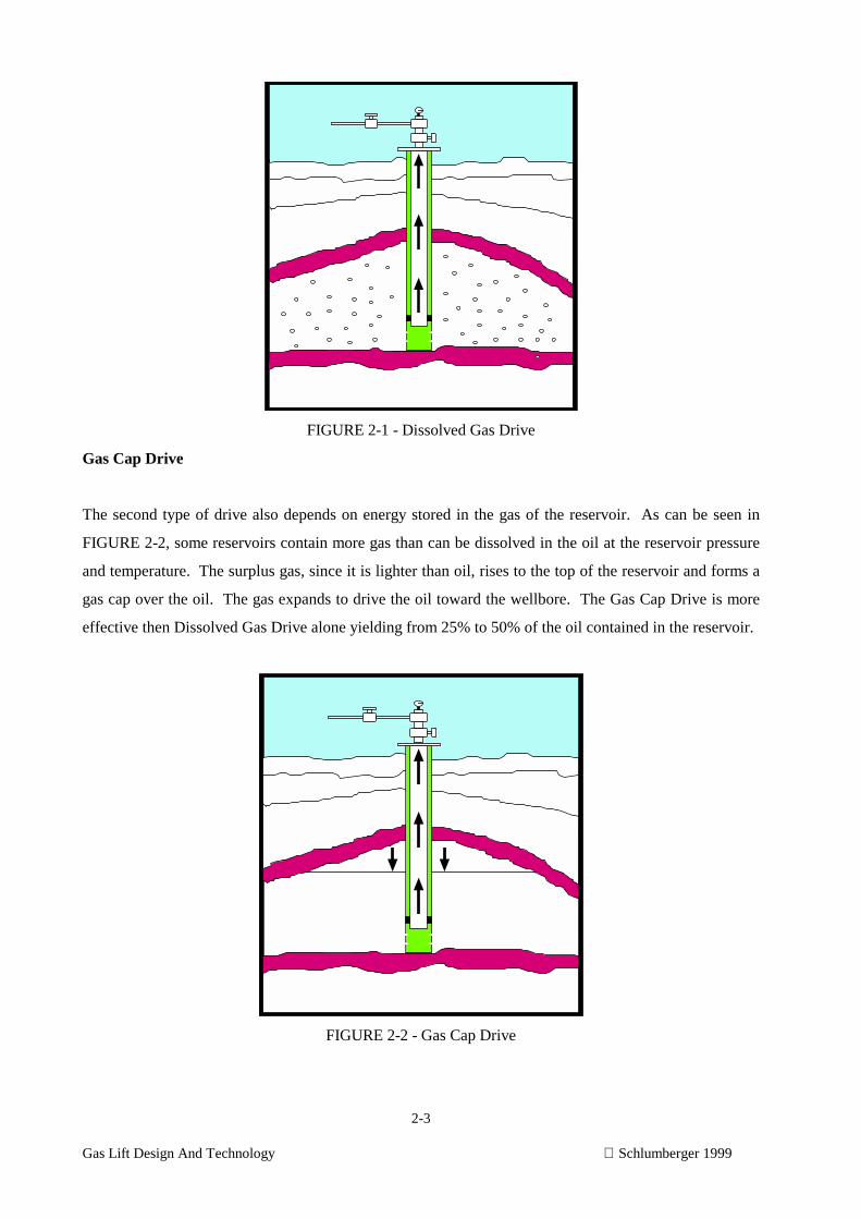
Dissolved Gas Drive
FIGURE 2-1 illustrates a dissolved gas drive. Oil has gas dissolved in it. As the gas escapes from the
oil, the bubbles expand and this explanation produces a force on the oil which drives it through the
reservoir toward the well and assists in lifting it to the surface. It is generally considered the least
effective type of drive yielding only 15% to 25% of the oil originally contained in the reservoir.
2-3
Gas Lift Design And Technology Schlumberger 1999
FIGURE 2-1 - Dissolved Gas Drive
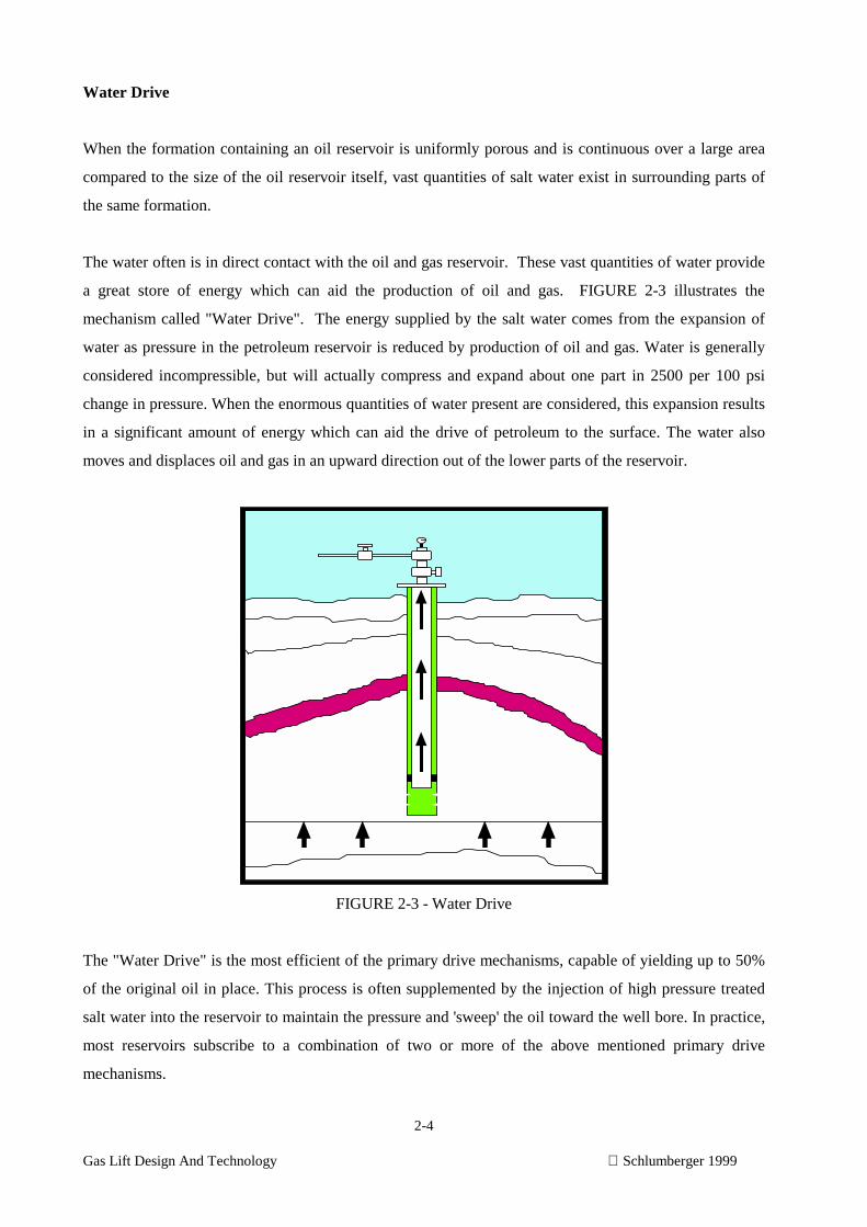
Gas Cap Drive
The second type of drive also depends on energy stored in the gas of the reservoir. As can be seen in
FIGURE 2-2, some reservoirs contain more gas than can be dissolved in the oil at the reservoir pressure
and temperature. The surplus gas, since it is lighter than oil, rises to the top of the reservoir and forms a
gas cap over the oil. The gas expands to drive the oil toward the wellbore. The Gas Cap Drive is more
effective then Dissolved Gas Drive alone yielding from 25% to 50% of the oil contained in the reservoir.
FIGURE 2-2 - Gas Cap Drive
2-4
Gas Lift Design And Technology Schlumberger 1999
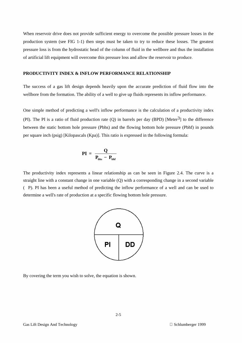
Water Drive
When the formation containing an oil reservoir is uniformly porous and is continuous over a large area
compared to the size of the oil reservoir itself, vast quantities of salt water exist in surrounding parts of
the same formation.
The water often is in direct contact with the oil and gas reservoir. These vast quantities of water provide
a great store of energy which can aid the production of oil and gas. FIGURE 2-3 illustrates the
mechanism called "Water Drive". The energy supplied by the salt water comes from the expansion of
water as pressure in the petroleum reservoir is reduced by production of oil and gas. Water is generally
considered incompressible, but will actually compress and expand about one part in 2500 per 100 psi
change in pressure. When the enormous quantities of water present are considered, this expansion results
in a significant amount of energy which can aid the drive of petroleum to the surface. The water also
moves and displaces oil and gas in an upward direction out of the lower parts of the reservoir.
FIGURE 2-3 - Water Drive
The "Water Drive" is the most efficient of the primary drive mechanisms, capable of yielding up to 50%
of the original oil in place. This process is often supplemented by the injection of high pressure treated
salt water into the reservoir to maintain the pressure and 'sweep' the oil toward the well bore. In practice,
most reservoirs subscribe to a combination of two or more of the above mentioned primary drive
mechanisms.
2-5
Gas Lift Design And Technology Schlumberger 1999
When reservoir drive does not provide sufficient energy to overcome the possible pressure losses in the
production system (see FIG 1-1) then steps must be taken to try to reduce these losses. The greatest
pressure loss is from the hydrostatic head of the column of fluid in the wellbore and thus the installation
of artificial lift equipment will overcome this pressure loss and allow the reservoir to produce.
PRODUCTIVITY INDEX & INFLOW PERFORMANCE RELATIONSHIP
The success of a gas lift design depends heavily upon the accurate prediction of fluid flow into the
wellbore from the formation. The ability of a well to give up fluids represents its inflow performance.
One simple method of predicting a well's inflow performance is the calculation of a productivity index
(PI). The PI is a ratio of fluid production rate (Q) in barrels per day (BPD) [Meter3] to the difference
between the static bottom hole pressure (Pbhs) and the flowing bottom hole pressure (Pbhf) in pounds
per square inch (psig) [Kilopascals (Kpa)]. This ratio is expressed in the following formula:
PI = Q
P Pbhs bhf−
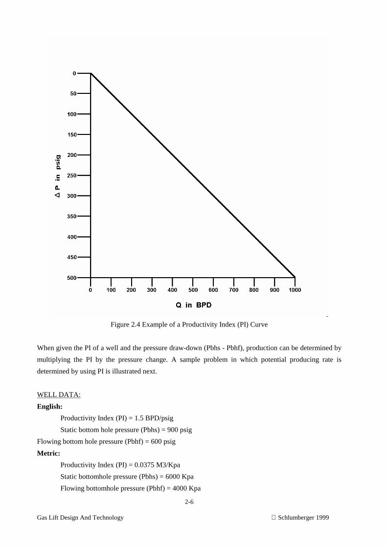
The productivity index represents a linear relationship as can be seen in Figure 2.4. The curve is a
straight line with a constant change in one variable (Q) with a corresponding change in a second variable
(�P). PI has been a useful method of predicting the inflow performance of a well and can be used to
determine a well's rate of production at a specific flowing bottom hole pressure.
By covering the term you wish to solve, the equation is shown.
2-6
Gas Lift Design And Technology Schlumberger 1999
Figure 2.4 Example of a Productivity Index (PI) Curve
When given the PI of a well and the pressure draw-down (Pbhs - Pbhf), production can be determined by
multiplying the PI by the pressure change. A sample problem in which potential producing rate is
determined by using PI is illustrated next.
WELL DATA:
English:
Productivity Index (PI) = 1.5 BPD/psig
Static bottom hole pressure (Pbhs) = 900 psig
Flowing bottom hole pressure (Pbhf) = 600 psig
Metric:
Productivity Index (PI) = 0.0375 M3/Kpa
Static bottomhole pressure (Pbhs) = 6000 Kpa
Flowing bottomhole pressure (Pbhf) = 4000 Kpa
2-7
Gas Lift Design And Technology Schlumberger 1999
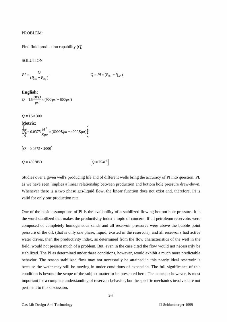
PROBLEM:
Find fluid production capability (Q)
SOLUTION
PIQ
P Pbhs bhf
=−( )
Q PI P Pbhs bhf= × −( )
English:
QBPD
psipsi psi= × −1 5 900 600. ( )
Q = ×1 5 300.
Metric:
QM
KpaKpa Kpa= × −
LNM
OQP
0 0375 6000 40003
. ( )
Q = ×0 0375 2000.
Q BPD= 450 Q M= 75 3
Studies over a given well's producing life and of different wells bring the accuracy of PI into question. PI,
as we have seen, implies a linear relationship between production and bottom hole pressure draw-down.
Whenever there is a two phase gas-liquid flow, the linear function does not exist and, therefore, PI is
valid for only one production rate.
One of the basic assumptions of PI is the availability of a stabilized flowing bottom hole pressure. It is
the word stabilized that makes the productivity index a topic of concern. If all petroleum reservoirs were
composed of completely homogeneous sands and all reservoir pressures were above the bubble point
pressure of the oil, (that is only one phase, liquid, existed in the reservoir), and all reservoirs had active
water drives, then the productivity index, as determined from the flow characteristics of the well in the
field, would not present much of a problem. But, even in the case cited the flow would not necessarily be
stabilized. The PI as determined under these conditions, however, would exhibit a much more predictable
behavior. The reason stabilized flow may not necessarily be attained in this nearly ideal reservoir is
because the water may still be moving in under conditions of expansion. The full significance of this
condition is beyond the scope of the subject matter to be presented here. The concept; however, is most
important for a complete understanding of reservoir behavior, but the specific mechanics involved are not
pertinent to this discussion.
2-8
Gas Lift Design And Technology Schlumberger 1999
A clear insight into the factors affecting PI can be understood by considering three reservoir
characteristics: the physical nature of the reservoir itself, the nature of the reservoir fluids, and the nature
of the reservoir drive mechanism.
Most reservoirs are composed of several beds often separated by impermeable layers of rock. These beds
are usually of different thickness and permeability's. They may or may not be continuous throughout a
given reservoir. It is apparent, therefore, that the productivity of a single well is a summation of the
productivity or capacity of the individual beds. It is known that the capacity of a reservoir containing a
series of interconnected beds under unstabilized conditions may be over four times greater than the same
reservoir when pressure stabilization is reached. This is obviously significant and should be given
foremost consideration when designing an installation for an extended period.
If the reservoir pressure is below the bubble point or saturation pressure, the P.I., as determined from
well test, is a very unreliable yardstick for estimation of the reservoir capacity for the particular well.
Since all three fluid phases exist: gas, oil, and water, the achievement of the steady state or stabilized
condition is then impossible. The effect of this condition on the PI can sometimes be neglected; however,
if the pressure draw-down is small compared to the absolute pressure of the reservoir. When it is realized
that 50 to 90 percent of the total pressure draw-down may be in the immediate vicinity of the well bore
(100 feet or so), then the heterogeneous character of the fluids flowing can be more easily visualized.
It is a commonly established principle of reservoir fluid flow that, as the saturation of a given fluid
increases, it will flow more readily. Therefore, as a given unit volume of liquid phase and gas phase in
the reservoir flow toward the well bore, the absolute pressure on the unit volume decreases more and
more with a corresponding increase in the proportion of gas phase to the liquid phase. This, in turn,
means that the reservoir begins to "deliver" the gas phase more readily than the liquid phase. The net
result in terms of the PI of the well is that for a given pressure draw-down a reasonable amount of oil
may be produced with a moderate GOR. However, if the pressure drop is doubled over what it was
before, one cannot expect to get twice the amount of stock tank oil as before.
This is stating in effect that the PI of a well is not a straight line function and that it will often vary with
producing rates. This is a very common problem in gas lift design. Many operators do not appreciate this
fundamental principle of reservoir behavior.
The reservoir drive mechanism influences the PI reliability to a very great extent. As used here, the term
drive mechanism is used to differentiate between reservoirs whose motive power is primarily a
displacement type as opposed to depletion type.
2-9
Gas Lift Design And Technology Schlumberger 1999
Displacement type refers to strong active water drive or gas cap drive, and depletion type refers to a
closed reservoir or one in which the motive power in the reservoir is primarily from the gas in solution in
the oil. The latter is commonly termed a volumetric reservoir. It should be apparent that reservoirs with
the displacement type drive will generally produce more reliable PIs from well tests than will the
depletion type. In the displacement type drive, there is little or no free gas (aside from that existing in a
gas cap) and; hence, the reservoir capability to deliver the single phase liquid is greater than it would be
if the free gas were present. Further, the deliver-ability will be more consistently uniform over a period of
time (or pressure decline). It must be pointed out, however, that under certain conditions there can be
serious limitations to PI determinations from this type of reservoir drive. If an individual well is pulled
too hard, then a localized depletion drive will result and obviously the PI, as determined, will not be
reliable for predicting the well performance.
This depletion type reservoir mechanism will yield fairly reliable PIs only when the pressure draw-down
is small compared to the shut-in reservoir pressure. This discussion of the productivity index does not
include certain other mechanical factors that contribute toward its unreliability. The manner in which the
well has been completed is very significant.
The PI not only changes with time or total production, but also changes with increased draw-down at any
one specific time in the life of the well. If we measure several PI's in a well during a specific time
interval, a relationship will be obtained between rate and flowing pressure which normally is not linear
for a solution gas drive field. This may be attributed to one or more of the following factors:
1. Increased gas saturation of the oil near the well bore can occur because of the reduced reservoir
pressure. This can lower the permeability of the formation to oil flow at the higher producing rates.
2. The flow may change from laminar (in thin layers) to turbulent in some of the flow capillaries near
the well bore at increased producing rates.
3. The critical flow rates through pores may be exceeded at the formation face in the well bore. These
pores act as orifices when the critical rate is exceeded. Increased draw-downs; therefore, have a
diminished effect on increasing rates.
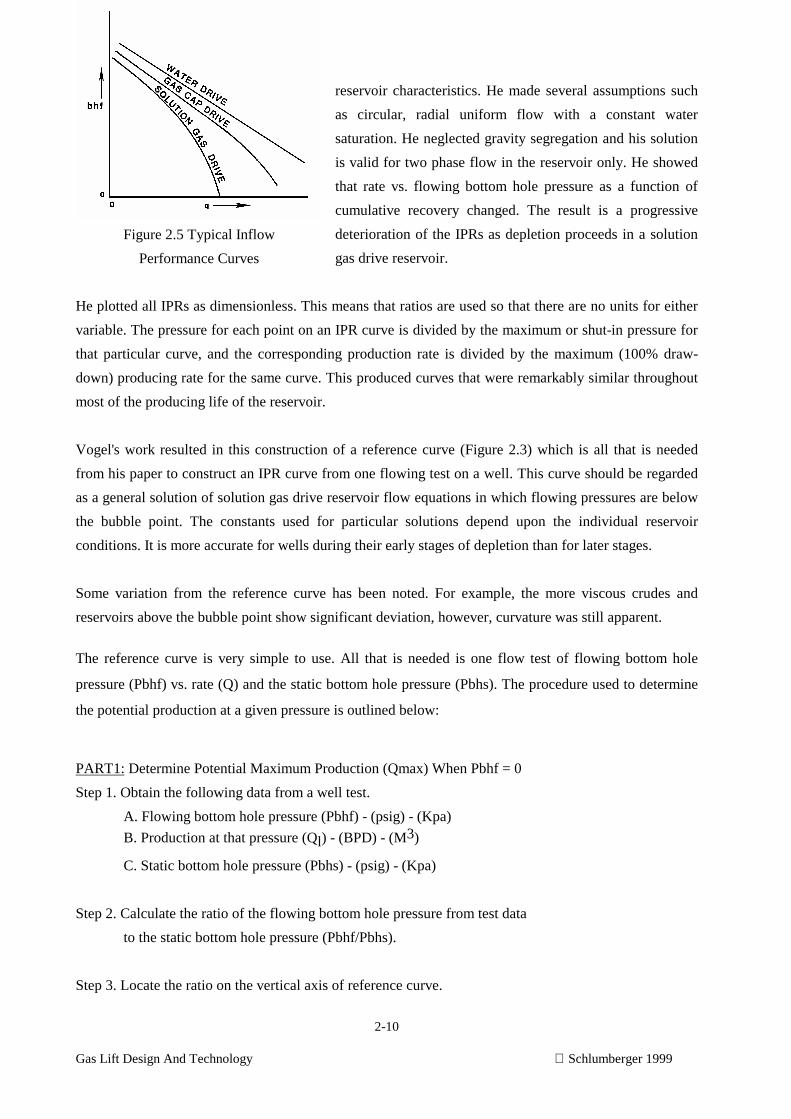
A second approach to the production of a well's performance is to plot production against flowing bottom
hole pressure. This plot of q vs. Pbhf is called an inflow performance curve and was first used byGilbert1, in describing well performance. Typical curves are illustrated in Figure 2.5 and differ
depending upon the type of reservoir. The curve for strong water drive is essentially a straight line as
discussed above under productivity index. The determination of the non-linear relationships observed forsolution gas drive wells presents a significant problem. A publication by Vogel2 in January, 1968 offered
a solution in determining an inflow performance curve for a solution gas drive for flow below the bubble
point. By use of a computer, he calculated inflow performance relationship (IPR) curves for wells
producing from several fictitious solution gas drive reservoirs that covered a wide range of oil and
2-10
Gas Lift Design And Technology Schlumberger 1999
reservoir characteristics. He made several assumptions such
as circular, radial uniform flow with a constant water
saturation. He neglected gravity segregation and his solution
is valid for two phase flow in the reservoir only. He showed
that rate vs. flowing bottom hole pressure as a function of
cumulative recovery changed. The result is a progressive
deterioration of the IPRs as depletion proceeds in a solution
gas drive reservoir.
He plotted all IPRs as dimensionless. This means that ratios are used so that there are no units for either
variable. The pressure for each point on an IPR curve is divided by the maximum or shut-in pressure for
that particular curve, and the corresponding production rate is divided by the maximum (100% draw-
down) producing rate for the same curve. This produced curves that were remarkably similar throughout
most of the producing life of the reservoir.
Vogel's work resulted in this construction of a reference curve (Figure 2.3) which is all that is needed
from his paper to construct an IPR curve from one flowing test on a well. This curve should be regarded
as a general solution of solution gas drive reservoir flow equations in which flowing pressures are below
the bubble point. The constants used for particular solutions depend upon the individual reservoir
conditions. It is more accurate for wells during their early stages of depletion than for later stages.
Some variation from the reference curve has been noted. For example, the more viscous crudes and
reservoirs above the bubble point show significant deviation, however, curvature was still apparent.
The reference curve is very simple to use. All that is needed is one flow test of flowing bottom hole
pressure (Pbhf) vs. rate (Q) and the static bottom hole pressure (Pbhs). The procedure used to determine
the potential production at a given pressure is outlined below:
PART1: Determine Potential Maximum Production (Qmax) When Pbhf = 0
Step 1. Obtain the following data from a well test.
A. Flowing bottom hole pressure (Pbhf) - (psig) - (Kpa)
B. Production at that pressure (Ql) - (BPD) - (M3)
C. Static bottom hole pressure (Pbhs) - (psig) - (Kpa)
Step 2. Calculate the ratio of the flowing bottom hole pressure from test data
to the static bottom hole pressure (Pbhf/Pbhs).
Step 3. Locate the ratio on the vertical axis of reference curve.
Figure 2.5 Typical Inflow
Performance Curves
2-11
Gas Lift Design And Technology Schlumberger 1999
Step 4. Find point on the reference curve.
Step 5. Locate the ratio of production at that bottom hole pressure to theproduction at 0 pressure (Q1 / Qmax).
Step 6. Solve for Qmax by dividing the value of Q1 by the ratio Q1 / Qmax.
PART 2 Determine Potential Production (Q2) At The Given Pbhf.
Step 7. Calculate the ratio of the given flowing bottom hole pressure to the static bottom hole pressure
(Pbhf/Pbhs).
Step 8. Locate the ratio on the vertical axis of the reference curve.
Step 9. Find the point on the reference curve.
Step 10. Locate the ratio of production at the given bottom hole ratio (Q2) to the production at 0 psig.
Step 11. Calculate production at the given bottom hole pressure (Q2) by multiplying the ratio times the
production when Pbhf = 0 (Qmax found in Step Number 6).
A sample problem is illustrated below
WELL DATA: EnglishMetric
Flowing bottom hole pressure (Pbhf) 600 psig 4135 Kpa
Production at Pbhf Q1 400 BPD 64 M3
Static bottom hole pressure (Pbhs) 900 psig 6205 Kpa
PROBLEM
Find potential maximum production (Qmax) when Pbhf= 500 psig / 3447 Kpa
SOLUTION:
PART 1
Determine Maximum Potential Production (Qmax) When Pbhf = 0
English Metric
Step 1. With Q1 @ Pbhf = 400 BPD 64M3
2-12
Gas Lift Design And Technology Schlumberger 1999
Step 2. P
Pbhf
bhs
====600
9000 67==== . 4135
62050 67==== .
Step 3. Using dimensionless inflow performance relationship curve for solution gas drive reservoir (after
Vogel). Enter the y axis at 0.67 proceed to the right until the IPR curve is met, proceed down from the
intercept of 0.67 (y - axis) and the IPR curve to the x - axis
Step 4. Using figure 2.3, read value from x - axis, 0.49.
Step 5. QQ
max .==== 1
0 49 400
0 49816
.==== 64
0 49131
.====
PART 2
Determine Potential Production (Q2) At The Given Pbhf (500 psig) [3447 Kpa]
English: Metric:
Step 6. P
Pbhf
bhs
==== 500
9000 56==== . 3447
62050 56==== .
Step 7. Using dimensionless inflow performance relationship curve for solution gas drive reservoir (after
Vogel).. Enter the y axis at 0.55 proceed to the right until the IPR curve is met, proceed down from the
intercept of 0.55 (y - axis) and the IPR curve to the x - axis
Step 8. Using figure 2.3, read value from x - axis, 0.65.
Step 9. Q Q2 65==== ××××max . 816 0 65 530×××× ====. 131 0 65 85×××× ====.
Although the problem above was solved using the reference curve, an IPR for a specific well can be
plotted when several points are known. For the purpose of this discussion, the general reference curve
can be used for your calculations.
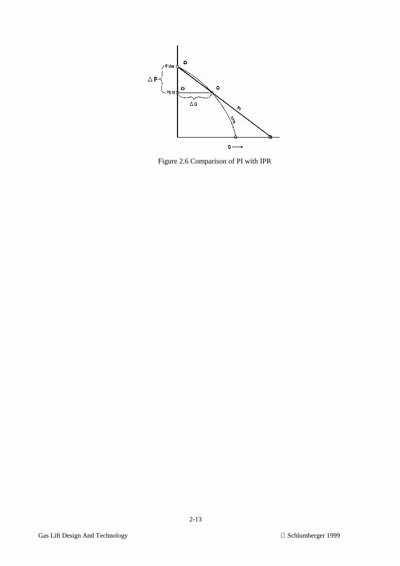
In summary, both PI and IPR can be used to determine a well's production. The producing rate will differ
depending on the method used. This is particularly true as the amount of draw-down is increased as can
be seen in Figure 2.6.
It is evident that IPR data more accurately reflects a well's inflow performance. The production,
therefore, can be more accurately determined.
2-13
Gas Lift Design And Technology Schlumberger 1999
Figure 2.6 Comparison of PI with IPR
2-14
Gas Lift Design And Technology Schlumberger 1999
References
1. Vogel, J.V.: “Inflow Performance Relationship for Solution-Gas Drive Wells”. J. Pet. Tech.(Jan 1968) 83.
2. Standing, M.B.: “Inflow Performance Relationships for Damaged Wells Producing by Solution-Gas Drive”. J. Pet. Tech. (Nov. 1970) 1399.
3. Fetkovich, M.J.: “The Isochronal Testing of Oil Wells”, paper SPE 4529 presented at theSPE - AIME 48th Annual Fall Meeting, Las Vegas, Nevada (Sept. 30 - Oct. 3, 1973).
4. Mathews, C.S. and Russell, D.G.: “Pressure Build-Up and Flow Test in Wells”, MonographSeries, SPE, Dallas (1976), 1,21.
5. Gilbert, W.E.: “Flowing and Gas Lift Well Performance”, Drill. and Prod. Prac., API (1954)126.
6. Eickmeier, J.R.:“How to Accurately Predict Future Well Productivities”, World Oil (May 1968)99.
7. Standing, M.B.: “Concerning the Calculation of Inflow Performance of Wells Producing fromSolution Gas Drive Reservoirs”, J. Pet. Tech. (Sept. 1971) 1141.

3 - 1Gas Lift Design And Technology Schlumberger 1999
GAS LIFT DESIGN AND TECHNOLOGY
3. Natural Gas Laws Applied to Gas Lift
3 - 2Gas Lift Design And Technology Schlumberger 1999
3. Natural Gas Laws Applied to Gas Lift
CHAPTER OBJECTIVE: Given all required data and the appropriate formula, you will
calculate gas pressure at depth, rate of flow through an orifice, the valve pressure set at
60°F for a given down hole temperature, and gas volumes within a closed conduit.
INTRODUCTION
The application of gas lift equipment requires the understanding of the behavior of gas. Although all
gases have common behaviors known as the natural gas laws, there are some differences between the
injection gas which is a mixture of several gases with different chemical properties and the nitrogen
which is used to charge pressure operated gas lift valves.
Designing a gas lift installation involves the determination of gas pressure in the casing or tubing at the
specific depth of a valve when the surface injection pressure is known. The designer must also be able to
determine the volume of gas that can be delivered to the tubing through a particular valve in order to
obtain the proper gas to liquid ratio needed to lift the fluids to the surface. Since the same pressure is set
at the surface under a standard temperature, the pressure must be corrected so that proper operating
pressure will exist at the down hole temperature.

3 - 3Gas Lift Design And Technology Schlumberger 1999
PROPERTIES OF INJECTION GAS
Natural gas injected into a well, as well as the dissolved gas in the reservoir fluid, is subject to a number
of gas laws. Gas, unlike liquids, is an elastic fluid. It is often defined as a homogeneous fluid which
occupies all the space in a container. This is easily visualized by noting, for example, that 1 lb. of liquid
placed in a closed container may fill a small portion of the total volume of that container. However, 1 lb.
of gas placed in the same empty container will fill the container completely.
Gases expand with increases in temperature and contract with decreases in temperature. The volume of
gases is inversely related to pressure. As the pressure increases, the gas volume decreases. Gas volume is
usually measured in standard cubic feet (scf) [NM3]. A standard cubic foot is defined as the volume
contained in one cubic foot if the pressure is 14.73 psia and if the temperature is 60°F. A "normalized"
cubic meter is defined as the volume contained in one cubic meter if the pressure is 101.32 KPa and if the
temperature is 0º Celsius. Note that a "standard" cubic meter is defined by contractual agreement and is
usually at a temperature of 20º C.
It is known that gases have weight similar to any other fluid. Air, for example, weighs 0.0764 lbs. per
cubic foot [1.2238 Kg/M3] at 14.7 psia [101.353 KPa] and 60º F [15.56º C]. On a comparative basis, gas
is always compared to air as a liquid is compared to water. The ratio of the density of a gas compared to
the density of air is known as the gas gravity or relative density.
One of the most important calculations required in gas lift designs is the determination of gas pressure at
a given depth.

3 - 4Gas Lift Design And Technology Schlumberger 1999
The equation for calculating pressure at depth is:
English Metric
P L P S e
S G L
T Z@ @
. .
.= ××
× ×FHG
IKJ53 34 P L P S e
L
T Z@ @ .= ××× ×
FHG
IKJ
γ29 28
Where:
e = 2.71828 e = 2.71828
P L@ = Pressure at depth, psia P L@ = Pressure at depth, kPa
P S@ = Pressure at surface, psia P S@ = Pressure at surface, kPa
SG = Gas Specific gravity γ = Gas relative density
L = Depth, feet L = Depth, meters
T = Average temperature, T = Average temperature, Kelvin
Degrees R
Z = Average Compressibility Z = Average Compressibility
for T and average pressure for T and average pressure
The average compressibility (Z ) is difficult to determine. Compressibility is based on the average
temperature and pressure and since the average temperature and pressure are unknown, the solution
becomes a repetitive trial and error procedure. A frequently used shortcut is to use a "rule of thumb"
equation. The equation below is based on a gas specific gravity of 0.65, a geothermal gradient at
1.6°F/100 ft. and a surface temperature of 70°F. This equation should only be used when well conditions
are close to these values.
English Metric
P L P SP S L
@ @ .@= + × ×2 3
100 1000P L P S
P S L@ @ .
@= + × ×15 65680 305
In addition to the "rule of thumb", gas lift designers frequently use charts like the one seen in Figure 3.1.
To use the chart, follow the procedure outlined below:
Step 1. Obtain surface pressure P@S.
Step 2. Locate P@S on vertical axis on Figure 1.
Step 3. Locate the line on graph representing the given depth across from that point
(Step 2).
Step 4. Locate P@L on Horizontal axis by dropping straight down from the line.

3 - 5Gas Lift Design And Technology Schlumberger 1999
Injection gas pressure at depth - English
3 - 6Gas Lift Design And Technology Schlumberger 1999
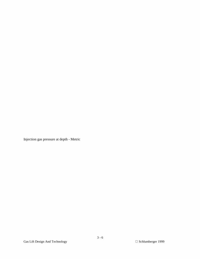
Injection gas pressure at depth - Metric

3 - 7Gas Lift Design And Technology Schlumberger 1999
When the well conditions differ from those given above, pressure at depth is deter-mined using charts
like those seen in Figures 3.2 and 3.3. The following data must be given:
1. Temperature at Surface (T@S) °F [°C]
2. Geothermal Gradient (G/T) °F/100 ft [°C/meter]
3. Specific Gravity (SG.) [Relative Density]
4. Pressure at Surface (P@S) psig [kPa]
5. Depth (L) feet [meters]
The following steps must be completed in order to determine the pressure at a given depth:
Step 1. Determine the temperature at depth by applying the following formula:English: Metric:
T L T STemp Grad L
@ @. .= + ×100
T L T S Temp Grad L@ @ .= + ×
Step 2. Calculate the average temperature:
TT L T S
avg =+@ @b g2
TT L T S
avg =+@ @b g2
Step 3. Estimate the P@L using the "rule of thumb" equation given above.
Step 4. Calculate the average pressure: Pavg = P@L + P@S
PP L P S
avg =+@ @b g2
PP L P S
avg =+@ @b g2
Step 5. Enter Figure 3.2 with the average temperature calculated in Step 2 on the left horizontal axis.
Travel up to the given gas gravity. Travel across the graph to the right.
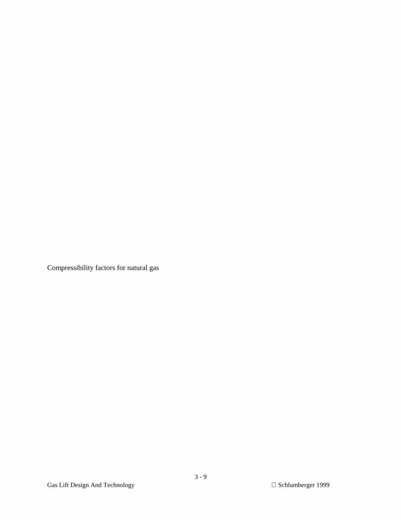
Step 6. Enter Figure 3.2 with the average pressure estimated in Step 4 and travel upward until the line
intersects the line drawn in Step 5. Read the compressibility factor at the point of intersection.
3 - 8Gas Lift Design And Technology Schlumberger 1999
Step 7. Enter Figure 3.3 with the given gas gravity and travel up to given depth. Travel across to the
average temperature calculated in Step 2. Travel down to the compressibility factor determined
in Step 6. Move across to the surface pressure line (P@S given) and down from this point to the
pressure at depth line. Read the P@L on the lower horizontal axis.
Step 8. Compare P@L with your estimate. If it differs by more than 10%, repeat the entire procedure
using the P@L just determined to calculate the average pressure in Step 4. Repeat the
procedure until the derived P@L becomes constant (at least 2 values for P@L).
3 - 9Gas Lift Design And Technology Schlumberger 1999
Compressibility factors for natural gas
3 - 10Gas Lift Design And Technology Schlumberger 1999
Gas pressure at depth
3 - 11Gas Lift Design And Technology Schlumberger 1999
VOLUME OF A GAS IN A CONDUIT
It is sometimes necessary to determine the volume of gas in a conduit under given conditions. This is
particularly true when designing conventional and chamber intermitting installations. Equations have
been derived to determine volume in a conduit and determine the gas required to change the pressure
within the conduit.
The internal capacity of a single circular conduit such as a tubing or casing string can be calculated using
the following equations:English Metric
Q (ft3 / 100 ft.) = 0.5454 di2 Q(m3 / 100 meters) = 0.007854 di2
Q (barrels/100 ft.) = 0.009714 di2)
Where:
di = the inside diameter in inches di = the inside diameter in cm
When it is necessary to determine the annular capacity of a tubing string inside casing, the equation
below can be used.
English Metric
Q(ft3 / 100 ft.) = 0.5454 (di2 - do2) Q(m3 / 100 meters = 0.007854(di2 - do2)
Q(barrels/100 ft.) = 0.09714 (di2 - do2)
Where:
di = the inside diameter in inches di = the inside diameter in cmdo = the outside diameter in inches do = the outside diameter in cm
Once the volume or capacity of a conduit has been determined, it is often necessary to find the volume of
gas contained in the conduit under specific well conditions. The equation below can be used for this
purpose:
b VP T
Z P Tb
b
= × ×× ×
Where:

3 - 12Gas Lift Design And Technology Schlumberger 1999
b = gas volume at base conditions
V = capacity of conduit in cubic ft. (see formula above)
P = average pressure within conduit (psia)
Tb = temperature base in degrees Rankin
Z = compressibility factor for average pressure and temperature in a conduit
(See Figure 3.2)
Pb = pressure base (14.73 psi)
T = average temperature in the conduit in degrees Rankin

3 - 13Gas Lift Design And Technology Schlumberger 1999
VOLUMETRIC GAS THROUGHPUT OF A CHOKE
Another important determination is the quantity of gas that can pass through a given opening during a
specific time period. In a gas lift installation, if sufficient gas will not pass through a particular port, the
required GLR cannot be obtained to lift fluids from a given depth. In gas lift design work, the rate of gas
flow is expressed in standard cubic feet over a unit of time.
Most gas passage calculations for valve port sizing are based on the Thornhill-Craver studies. The
equation is:
QC A P g
kk
r r
G T
dk k k
=× × × ×
−× −
×
+155 211
2 1/ /a f a f
Where :
Q = Gas flow in 1000 scfd (MCFD) at 60 Deg. F. and 14.7 psia
Cd = Discharge coefficient
A= Area of opening, square inches
P1 = Upstream pressure, psia
P2 = Downstream pressure, psia
g = Acceleration of gravity, = 32.2 ft./sec.2
K = =Ratio C
C
Specific heat at constant pressure
Specific heat at constant volumep
v
r = Ratio P
P r2
1o≥
ro =2
k + 1
k / k−1( )
= Critical Flow Pressure Ratio
G = Specific gravity Air = 1( )T = Inlet temperature, Deg. R.
Since the equation above is so complex and its calculation is very time consuming, the chart in Figure 3.4
provides a means of quickly obtaining an approximate gas passage rata for a given port size. It must be
remembered, when using the chart, that a correction factor should be used. Since gas passage through a
gas lift valve occurs downhole, the chart must be corrected for specific gravity and temperature at the
valve depth.
To determine the gas passage rate using the chart and correction factors use the following procedure:
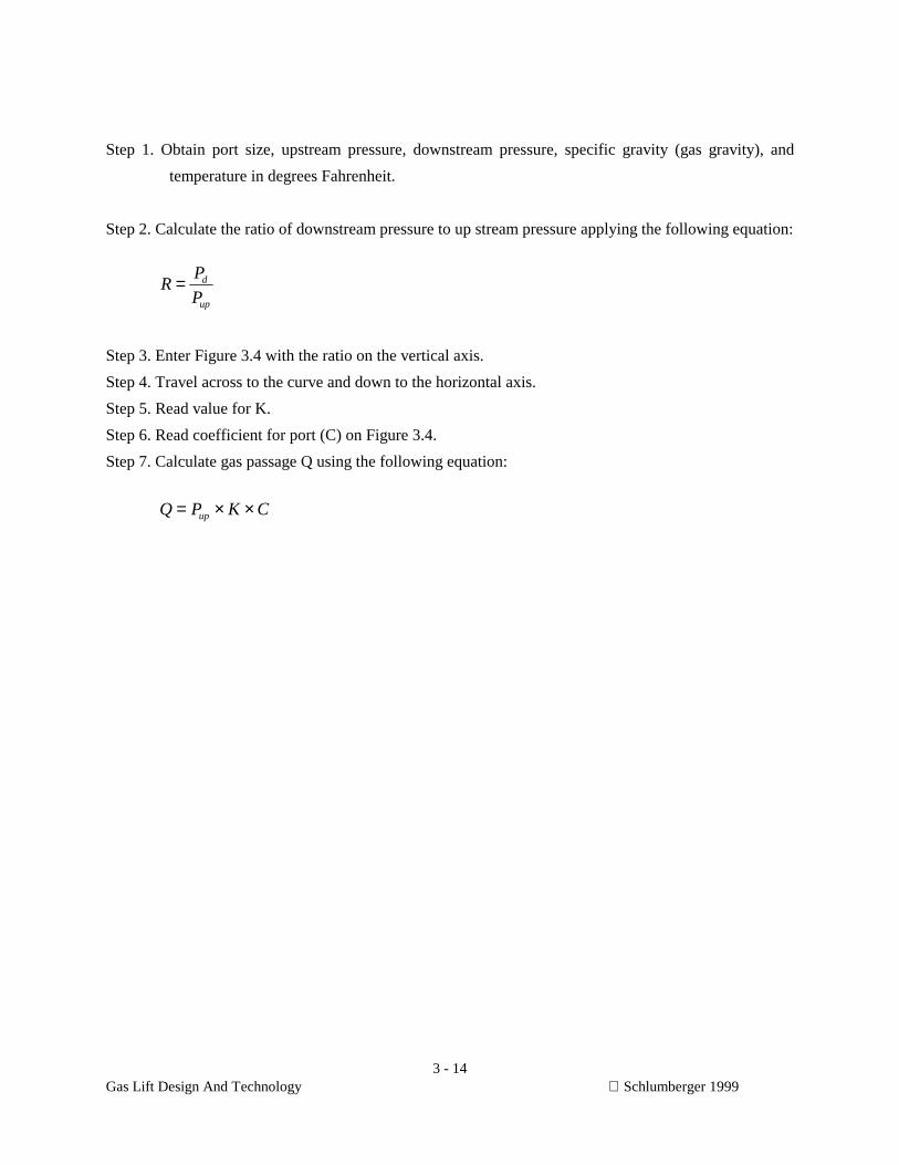
3 - 14Gas Lift Design And Technology Schlumberger 1999
Step 1. Obtain port size, upstream pressure, downstream pressure, specific gravity (gas gravity), and
temperature in degrees Fahrenheit.
Step 2. Calculate the ratio of downstream pressure to up stream pressure applying the following equation:
RP
Pd
up
=
Step 3. Enter Figure 3.4 with the ratio on the vertical axis.
Step 4. Travel across to the curve and down to the horizontal axis.
Step 5. Read value for K.
Step 6. Read coefficient for port (C) on Figure 3.4.
Step 7. Calculate gas passage Q using the following equation:
Q P K Cup= × ×
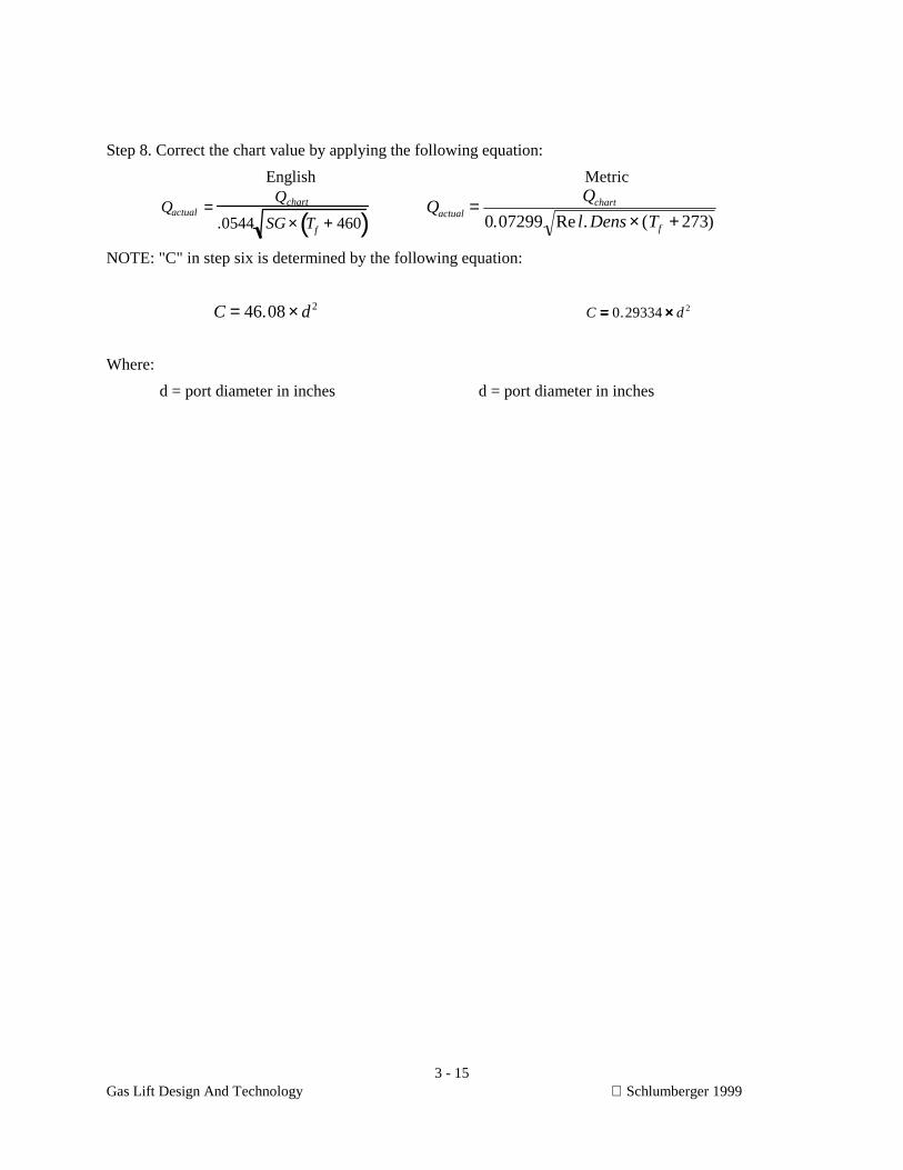
3 - 15Gas Lift Design And Technology Schlumberger 1999
Step 8. Correct the chart value by applying the following equation:
English Metric
Qactual =Qchart
.0544 SG × Tf + 460( )Q
Q
l Dens Tactual
chart
f
=× +0 07299 273. Re . ( )
NOTE: "C" in step six is determined by the following equation:
C d= ×46 08 2. C d==== ××××0 29334 2.
Where:
d = port diameter in inches d = port diameter in inches

3 - 16Gas Lift Design And Technology Schlumberger 1999
page reserved for Thornhill-Craver gas passage chart - English
3 - 17Gas Lift Design And Technology Schlumberger 1999
This page reserved for gas passage chart - Metric

3 - 18Gas Lift Design And Technology Schlumberger 1999
PROPERTIES OF NITROGEN
Most gas lift valves using a pressure charged bellows are filled with nitrogen. Therefore, special
consideration is given to this gas. Nitrogen has advantages over other potential gases to be used in
pressure charged bellows. It is readily available, non-corrosive, and non-explosive. In addition, the
compressibility of nitrogen and its temperature changes are predictable.
Like all other gases, when the temperature of nitrogen is increased and the volume held constant, the
pressure will increase. When the pressure of a valve is set at the test bench at 60°F [15�C�, the pressure
of the valve will be higher downhole where the temperature is greater. This increase in pressure due to
temperature increase can be approximated by the following equation:
P P Tc2 1= ×
Where:
P1 = Pressure at initial temperature
P2 = Pressure resulting from change of temperature
Tc = Temperature correction factor
and
English: Metric:
Tc =1+ .00215× T2 − 60( )1 + .00215 × T1 − 60( ) T
T
Tc ====++++ ××××++++ ××××
94195 387
94195 3872
1
Where:
T1 = Initial temperature, Deg. F. T1 = Initial temperature, Deg. C.
T2 = Present temperature, Deg. F. T2 = Present temperature, Deg. C.
When valves are set at a certain constant temperature, a table may be made for ease in applying
temperature corrections. For example, if all valves are to be charged with nitrogen when they are at 60°F
[15°C], a correction for temperature (at well depth) may be created using the following equation:
English: Metric:
Ct =1
1+ .00215× T @ L − 60( ) Ct =100000
94195+ 387× T1
Where:

3 - 19Gas Lift Design And Technology Schlumberger 1999
Ct = Correction for temperature
T L@ = Temp at valve depth, °F. T L@ = Temp at valve depth, °C.
Then: P C Pb t bt= ×bg
Where:
Pb = Bellows pressure at 60°F., psig Pb = Bellows pressure at 15°C., kPa
Pbt = Bellows pressure at valve depth Pbt = Bellows pressure at valve depth
temp, psig temp, psig
Table 3.1A contains the correction for temperature (Ct) for temperatures from 60°F to 300°F. Table 3.1B
contains the correction for temperature (Ct) for temperatures from 16°C to 150°C. These tables should be
readily available for problems requiring the determination of dome pressure. Since it is based on the most
frequently used pressures and temperatures, it should be limited to use with moderate temperature
corrections. It is not accurate at extreme pressures and temperatures.
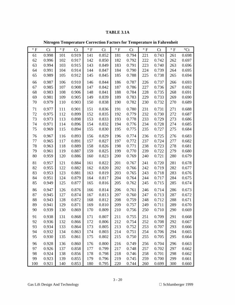
3 - 20Gas Lift Design And Technology Schlumberger 1999
TABLE 3.1A
Nitrogen Temperature Correction Factors for Temperature in Fahrenheit
° F Ct ° F Ct ° F Ct ° F Ct ° F Ct ° F °Ct61 0.998 101 0.919 141 0.852 181 0.794 221 0.743 261 0.69862 0.996 102 0.917 142 0.850 182 0.792 222 0.742 262 0.69763 0.994 103 0.915 143 0.849 183 0.791 223 0.740 263 0.69664 0.991 104 0.914 144 0.847 184 0.790 224 0.739 264 0.69565 0.989 105 0.912 145 0.845 185 0.788 225 0.738 265 0.694
66 0.987 106 0.910 146 0.844 186 0.787 226 0.737 266 0.69367 0.985 107 0.908 147 0.842 187 0.786 227 0.736 267 0.69268 0.983 108 0.906 148 0.841 188 0.784 228 0.735 268 0.69169 0.981 109 0.905 149 0.839 189 0.783 229 0.733 269 0.69070 0.979 110 0.903 150 0.838 190 0.782 230 0.732 270 0.689
71 0.977 111 0.901 151 0.836 191 0.780 231 0.731 271 0.68872 0.975 112 0.899 152 0.835 192 0.779 232 0.730 272 0.68773 0.973 113 0.898 153 0.833 193 0.778 233 0.729 273 0.68674 0.971 114 0.896 154 0.832 194 0.776 234 0.728 274 0.68575 0.969 115 0.894 155 0.830 195 0.775 235 0.727 275 0.684
76 0.967 116 0.893 156 0.829 196 0.774 236 0.725 276 0.68377 0.965 117 0.891 157 0.827 197 0.772 237 0.724 277 0.68278 0.963 118 0.889 158 0.826 198 0.771 238 0.723 278 0.68179 0.961 119 0.887 159 0.825 199 0.770 239 0.722 279 0.68080 0.959 120 0.886 160 0.823 200 0.769 240 0.721 280 0.679
81 0.957 121 0.884 161 0.822 201 0.767 241 0.720 281 0.67882 0.955 122 0.882 162 0.820 202 0.766 242 0.719 282 0.67783 0.953 123 0.881 163 0.819 203 0.765 243 0.718 283 0.67684 0.951 124 0.879 164 0.817 204 0.764 244 0.717 284 0.67585 0.949 125 0.877 165 0.816 205 0.762 245 0.715 285 0.674
86 0.947 126 0.876 166 0.814 206 0.761 246 0.714 286 0.67387 0.945 127 0.874 167 0.813 207 0.760 247 0.713 287 0.67288 0.943 128 0.872 168 0.812 208 0.759 248 0.712 288 0.67189 0.941 129 0.871 169 0.810 209 0.757 249 0.711 289 0.67090 0.939 130 0.869 170 0.809 210 0.756 250 0.710 290 0.669
91 0.938 131 0.868 171 0.807 211 0.755 251 0.709 291 0.66892 0.936 132 0.866 172 0.806 212 0.754 252 0.708 292 0.66793 0.934 133 0.864 173 0.805 213 0.752 253 0.707 293 0.66694 0.932 134 0.863 174 0.803 214 0.751 254 0.706 294 0.66595 0.930 135 0.861 175 0.802 215 0.750 255 0.705 295 0.664
96 0.928 136 0.860 176 0.800 216 0.749 256 0.704 296 0.66397 0.926 137 0.858 177 0.799 217 0.748 257 0.702 297 0.66298 0.924 138 0.856 178 0.798 218 0.746 258 0.701 298 0.66299 0.923 139 0.855 179 0.796 219 0.745 259 0.700 299 0.661
100 0.921 140 0.853 180 0.795 220 0.744 260 0.699 300 0.660
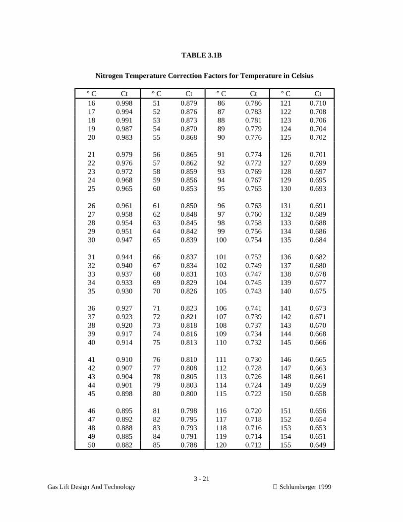
3 - 21Gas Lift Design And Technology Schlumberger 1999
TABLE 3.1B
Nitrogen Temperature Correction Factors for Temperature in Celsius
° C Ct ° C Ct ° C Ct ° C Ct16 0.998 51 0.879 86 0.786 121 0.71017 0.994 52 0.876 87 0.783 122 0.70818 0.991 53 0.873 88 0.781 123 0.70619 0.987 54 0.870 89 0.779 124 0.70420 0.983 55 0.868 90 0.776 125 0.702
21 0.979 56 0.865 91 0.774 126 0.70122 0.976 57 0.862 92 0.772 127 0.69923 0.972 58 0.859 93 0.769 128 0.69724 0.968 59 0.856 94 0.767 129 0.69525 0.965 60 0.853 95 0.765 130 0.693
26 0.961 61 0.850 96 0.763 131 0.69127 0.958 62 0.848 97 0.760 132 0.68928 0.954 63 0.845 98 0.758 133 0.68829 0.951 64 0.842 99 0.756 134 0.68630 0.947 65 0.839 100 0.754 135 0.684
31 0.944 66 0.837 101 0.752 136 0.68232 0.940 67 0.834 102 0.749 137 0.68033 0.937 68 0.831 103 0.747 138 0.67834 0.933 69 0.829 104 0.745 139 0.67735 0.930 70 0.826 105 0.743 140 0.675
36 0.927 71 0.823 106 0.741 141 0.67337 0.923 72 0.821 107 0.739 142 0.67138 0.920 73 0.818 108 0.737 143 0.67039 0.917 74 0.816 109 0.734 144 0.66840 0.914 75 0.813 110 0.732 145 0.666
41 0.910 76 0.810 111 0.730 146 0.66542 0.907 77 0.808 112 0.728 147 0.66343 0.904 78 0.805 113 0.726 148 0.66144 0.901 79 0.803 114 0.724 149 0.65945 0.898 80 0.800 115 0.722 150 0.658
46 0.895 81 0.798 116 0.720 151 0.65647 0.892 82 0.795 117 0.718 152 0.65448 0.888 83 0.793 118 0.716 153 0.65349 0.885 84 0.791 119 0.714 154 0.65150 0.882 85 0.788 120 0.712 155 0.649
2-21
Gas Lift Design And Technology Schlumberger 1999
OUTFLOW PERFORMANCE
The outflow performance describes the relationship between the surface flowrate and pressure drop in
the tubing. The prediction of this relationship is complicated by the multi-phase nature of the fluids.
Analysis of the outflow performance therefore requires the prediction of phase behavior, flowing
temperatures, effective fluid density and frictional pressure losses. The results of the outflow
performance are usually presented graphically. The most common plot depicts how the flowing bottom
hole pressure (Pbhf), varies with flowrate for a fixed back pressure (usually the wellhead or separator
pressure). The resulting curves are termed tubing performance curves (TPC) or lift curves. Any point on
the curve gives the pressure required at bottom hole conditions, Pwf, to achieve the given surface
flowrate against a specified back pressure.
VERTICAL AND HORIZONTAL MULTIPHASE FLOW
The pressure of fluids in the tubing and flow line is subject to changes in pressure. Since the fluids are a
mixture and because of the large number of factors involved, calculating the fluid pressure at a given
point is a very difficult task. The proper design of gas lift installation requires this information so
solutions to this problem are necessary.
Mathematical solutions have been developed which allow the designer to arrive at a specific pressure
gradient curve for the well. The available well data is fed into a computer which constructs the curve.
Since all data is not known, the curve is approximate but can be used for most design work.
Without computer curves, existing published curves can be matched with well data. These "working"
curves are applied to the solution of numerous problems. The data obtained from these curves are
accurate estimates when they are read with great care.
As fluids flow from the reservoir to the wellbore and eventually to the surface through the production
system, there is a continual pressure drop. This pressure drop is not constant throughout the system and is
caused by many factors. The fluid moving through the system actually may consist of three different
fluids (gas, water and oil) flowing at three different velocities. This movement of free gases and liquids
at the same time is called multiphase flow.
Multiphase flow can be divided into four categories depending on the direction of movement. As can be
seen in Figure 2.7, most production systems include: vertical multiphase flow, horizontal multiphase
flow, inclined multiphase flow, and directional multiphase flow. For the purposes of our discussion, we
will consider only vertical and horizontal flow.
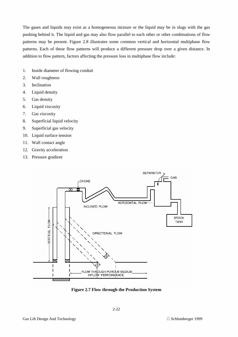
2-22
Gas Lift Design And Technology Schlumberger 1999
The gases and liquids may exist as a homogeneous mixture or the liquid may be in slugs with the gas
pushing behind it. The liquid and gas may also flow parallel to each other or other combinations of flow
patterns may be present. Figure 2.8 illustrates some common vertical and horizontal multiphase flow
patterns. Each of these flow patterns will produce a different pressure drop over a given distance. In
addition to flow pattern, factors affecting the pressure loss in multiphase flow include:
1. Inside diameter of flowing conduit
2. Wall roughness
3. Inclination
4. Liquid density
5. Gas density
6. Liquid viscosity
7. Gas viscosity
8. Superficial liquid velocity
9. Superficial gas velocity
10. Liquid surface tension
11. Wall contact angle
12. Gravity acceleration
13. Pressure gradient
Figure 2.7 Flow through the Production System

2-23
Gas Lift Design And Technology Schlumberger 1999
Figure 2.8 Multiphase Flow Patterns
Since the pressure drop is caused by a complex interaction of many factors, one of the major problems in
analyzing flowing wells and designing gas lift installations has been the prediction of flowing pressure at
depth. It is also important to understand the pressure drop in the horizontal flow line in order to
determine the back pressure at the wellhead. This problem has been the subject of numerous studies.
2-24
Gas Lift Design And Technology Schlumberger 1999
In 1939, E.C. Babson1 published a paper on vertical multiphase flow. W.E. Gilbert2 did a considerable
amount of work in 1939 and 1940 on vertical multiphase flow. However, he did not report his work until
1954. Gilbert's very important contribution to the state of the art is the pressure depth plot that is called
the gradient curve.
Poettmann-Carpenter3 published their paper in 1952. Their work resulted in a correlation rather than a
set of gradient curves. It was the first fundamental mathematical approach which gave good results over a
rather wide range of flowing conditions. Gradient curves plotted from calculations made according to the
Poettmann-Carpenter correlation have been widely used in the design of gas lift installations. The
correlation is good for 2- 3/8" and 2-7/8" tubing for flow rates between about 300 BPD and 2500 BPD.
Figure 4.3 is an example of such a flowing pressure gradient based on this correlation. Notice that the
curves are valid only under the conditions stated on the curve.
More recently there have been several other investigators publish general correlations. Of these, thebetter known correlations are the Hagedorn and Brown4, Orkiszewski5 and Ros6 '
The vertical multiphase flow correlations are accurate enough to be very useful to production personnel.
They have been used to accomplish the following functions:
1. Select correct tubing sizes (tubing or annular flow).
2. Predict when a well will quit flowing and require artificial lift.
3. Design artificial lift systems.
4. Determine flowing bottom hole pressures.
5. Determine Pl's of wells.
6. Predict maximum flow rates.
There are two methods by which vertical multiphase flow correlations can be used by production
personnel. The calculation can be made by computer or "published curves" (see Figure 4.3) can be used.
Most companies have at least one program available for vertical multiphase flow, and there are numerous
sets of published curves available.
When possible, the computer calculations are recommended but there are numerous occasions when
published curves must be used.
All vertical gradient curves have certain limitations. The fluids must be free of emulsions. At the present
time there is no way to predict the pressure losses that occur with emulsions. The tubing must be
unrestricted. The tubing string should be free of scale and paraffin build up. Mashed or kinked joints
must not exist in order for the vertical gradient curves to be accurate. The flow pattern must be relatively
stable. There should be no severe heading or slugging where there is several hundred psi between
maximum and minimum tubing pressures.
2-25
Gas Lift Design And Technology Schlumberger 1999
The well must be essentially vertical. The correlations do not take into consideration deviated holes. The
use of drilled depth results in pressures that are too great and the use of true vertical depth results in
pressures that are too low.
The calculation of pressure loss in flow lines requires a horizontal multiphase flowing pressure gradient.One such gradient is based on a paper by Eaton3 et al, in which data was obtained for horizontal flow
over several conditions including different pipe diameters and lengths.
When vertical flowing pressure gradients are compared with horizontal flowing pressure gradients one
obvious and important difference can be observed. As the Gas to Liquid Ratio (GLR) increases on the
vertical gradient, the pressure drop decreases, but with increased GLR in the horizontal gradient the
pressure drop increases. This can create problems for the gas lift designer. If the GLR produced by the
injected gas necessary to lift the fluids reaches high enough values, the increased pressure drop in the
flow line may actually cause loss in production. Only through a complete understanding of multiphase
flow through vertical and horizontal conduits, can a gas lift system be designed to operate efficiently.
Some of the correlation’s most widely accepted in the industry are:
• Duns and Ros (1963)
• Hagedorn and Brown (1967)
• Orkiszewski (1967)
• Aziz, Govier and Fogarasi (1972)
• Beggs and Brill (1973)
These correlations are available in most computer software used for predicting outflow performance.
Modifications have been made to some of these correlations in an attempt to improve their predictions.
These correlation’s predict different pressure drops for the same application. Any one of these
correlation’s or modifications may be successful for a given field. Validation with actual field data in the
form of flowing surveys is the only reliable method for choosing a pressure loss prediction method. In the
North Sea the Hagedorn and Brown modified correlation generally gives the best fit to measured data.
Calculation Background Information (reproduced courtesy of Edinburgh Petroleum Services Ltd.)
This section serves as a brief technical reference for the engineering calculations in WellFlo . Where
modification work has been carried out in-house, it is explained briefly here.
2-26
Gas Lift Design And Technology Schlumberger 1999
Pressure Drop Correlation’s
There are a number of pressure drop correlations in WellFlo . Six are basically taken from standard
theory, four have been modified in various ways (variants of the Duns and Ros, Beggs and Brill and
Hagedorn and Brown correlation’s), and two are hybrids (Dukler-Eaton-Flanigan and Barnea-Ansari-
Xiao (BAX)). The standard forms of the correlations follow the published references as closely as
possible. The BAX correlation is mechanistic.
There are three sources of pressure drop:
• Hydrostatic Gradient which arises from the density of the multi-phase column of fluids. It is
calculated from a knowledge of the liquid hold-up (the proportion of the flowing area occupied by
liquid), and the densities of the phases. It is proportional to the cosine of the deviation, being zero in
a horizontal pipe. Most correlations use a flow-regime map to determine the type of flow, and then
use a particular correlation for the flow regime concerned to determine hold-up.
• Friction Gradient arising from the drag of the fluids on the walls of the pipe. This is calculated in a
specific way for each correlation, but generally uses the concept of a Friction Factor diagram (such as
Moody’s) to calculate the friction factor as a function of the Reynolds Number and pipe roughness.
The friction factor is used to calculate the friction pressure gradient.
• Acceleration Gradient arising from the increasing kinetic energy of the fluids as they expand and
accelerate with decreasing pressure. This term is often negligible, but is always included in these
correlation's. All correlation's in WellFlo use an acceleration term proposed by Beggs and Brill based
on the mean phase velocities in each computational segment.
Each correlation is described in terms of these three pressure gradient components. Note that, for the
frictional gradient, the following correlation’s do not use the wall roughness entered in the component
dialog box, but compute their own roughness factors internally: Beggs and Brill, Beggs and Brill (no-
slip), Fancher-Brown, Dukler-Eaton-Flanigan.
• Duns and Ros follows the methods described by Brown. The correlation makes use of a flow
regime map covering bubble, slug and mist flow. There is a linear transition between slug and mist.
Each regime has its own holdup correlation. Holdup is not changed by deviation. Friction is
calculated with liquid properties for bubble and slug flow, and gas properties for mist. In mist flow,
wall friction is increased due to liquid ripples on the pipe wall.
2-27
Gas Lift Design And Technology Schlumberger 1999
• Duns and Ros (modified) has a flow regime map extended by the work of Gould et al. This
includes a new transition region between bubble and slug flow, and an additional froth flow region at
high flow rates. The holdup is considered as no-slip for froth flow, and is interpolated over the
bubble-slug transition. The other holdup relationships are as for the standard Duns and Ros. To
model deviation, the calculated holdup is modified using the Beggs and Brill corrections (see below).
Friction is calculated by the method proposed by Kleyweg. This uses a monophasic friction factor
rather than two-phase, but involves use of an average fluid velocity. This is claimed by Kleyweg to
be a better method.
• Beggs and Brill again follows the methodology outlined by Brown. This correlation is unique in
that it is based on a flow regime map for horizontal flow, from which a regime is first determined as
if the flow were horizontal. A horizontal holdup is then calculated by correlations. Lastly, this
holdup is corrected for the actual angle of deviation. Beggs and Brill’s correlation models up- and
down-flow. It is therefore recommended for all pipeline applications. However, since it was not
derived for vertical flow, it must be used with caution in vertical wells. Friction calculations in
Beggs and Brill use an internally defined two-phase smooth pipe friction factor. This may be
expected to under-estimate friction in rough pipes.
• Beggs and Brill (no-slip) uses the same methodology as the standard Beggs and Brill, with the
exception that the holdup used is not the horizontal holdup described above, but simply the no-slip
holdup, without deviation correction.
• Beggs and Brill (modified) also uses the same methodology as the standard Beggs and Brill, with
the following changes. There is no extra flow regime of froth flow, which (as in Duns and Ros
(modified)) assumes a no-slip holdup. This is triggered by highly turbulent flow. The friction factor
is changed from the smooth pipe model to the method used in Duns and Ros (modified) - a single-
phase friction factor using pipe roughness and average fluid velocity.
• Hagedorn and Brown again is as per Brown, with the modifications to Hagedorn and Brown’s
original work as recommended by them. These are: the use of the Griffith and Wallis correlation for
bubble flow (using a simplified flow regime map to detect bubble flow); and the use of no-slip
holdup if it gives greater density than Hagedorn and Brown’s correlation. There is no change to
holdup with deviation. A two-phase friction factor using pipe roughness is used.
• Hagedorn and Brown (modified) involves the adjustment of the standard Hagedorn and Brown
holdup for deviation using the Beggs and Brill correction. When Griffith and Wallis’ holdup
2-28
Gas Lift Design And Technology Schlumberger 1999
correlation is invoked (in bubble flow), it is also corrected. Otherwise, this is the same as the
standard Hagedorn and Brown correlation.
• Fancher and Brown is a no-slip correlation1, with no flow regime map. It has its own friction factor
model, which is independent of pipe roughness. This correlation cannot be recommended for general
use. According to Brown, it is only suitable for 2-3/8 - 2-7/8 inch tubing. It is included for any
historical comparisons which may be required. Generally, it differs widely from the results of the
other seven correlations.
• Orkizewski is again based on the description by Brown. This is perhaps the most sophisticated
correlation, as it uses the work of Duns and Ros and Griffith and Wallis, for mist and bubble flow
respectively (using a flow regime map similar to Duns and Ros’). It has its own correlation in the
slug flow region, which is based on the approach of Griffith and Wallis. A transition between slug
and mist flow is also modeled. The holdup is adjusted for deviation using the Beggs and Brill
correlation (as in the modified Duns and Ros and Hagedorn and Brown correlation’s). The friction
factor calculation uses wall roughness but varies with flow regime, and for mist flow retains the
Duns and Ros extra friction due to ripples in the film of liquid on the wall.
• Gray: this is a widely recommended correlation6 for gas and condensate systems which are
predominantly gas phase (with liquid entrained as droplets). No flow regime map is used, flow being
treated as pseudo-single phase. Water or liquid condensate is considered to adhere to the pipe wall,
resulting in a modified roughness term.
• Dukler-Eaton-Flanigan is a hybrid of the Dukler friction component and Flanigan correlation for
the hydrostatic component. A mixture density is calculated using Dukler’s equation, but with
Eaton’s holdup definition, and this is used in Dukler’s friction term. The liquid density is used in the
Flanigan hydrostatic term. The acceleration component is modeled with the Beggs and Brill
correlation. This correlation is not suitable for downflow.
• BAX (Barnea-Ansari-Xiao) correlation is ‘mechanistic’ in that is has been formulated largely on
physical modeling principles. It is applicable to all fluid types, in all sizes of pipe at any inclination.
• Flow regimes are predicted according to Barnea. Xiao’s model is used to compute the hydrostatic
and frictional pressure gradients for stratified flow, and Ansari’s model for all other flow regimes.
Hasan’s corrections for deviation from the horizontal or vertical are applied to these model where
necessary.
2-29
Gas Lift Design And Technology Schlumberger 1999
Combining the IPR and TPC Curves
After the IPR and TPC curves have been established for a given set of conditions, they are usually
presented on the same plot.
The intersection of the IPR and TPC can be used to predict the flowrate of a well at a given set of stable
flow conditions. Changing system parameters such as tubing ID, reservoir pressure, water cut, flowing
well head pressure or Gas Liquid Ratio affect either or both the IPR and the TPC, and hence alters the
wells production rate. Systematically varying the different system parameters allows one to compare the
incremental effects on production. In Figures 2-9 a & b the gas lift injection rate has been systematically
increased and the resulting effect on production can be used to produce a well performance curve for use
in optimizing gas injection rates see Figure 2-10.
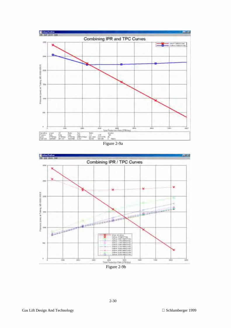
2-30
Gas Lift Design And Technology Schlumberger 1999
Figure 2-9a
Figure 2-9b
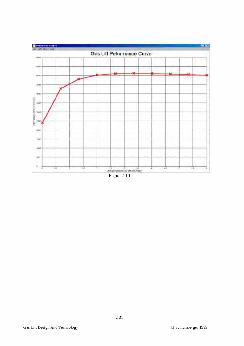
2-31
Gas Lift Design And Technology Schlumberger 1999
Figure 2-10
3 - 1Gas Lift Design And Technology Schlumberger 1999
GAS LIFT DESIGN AND TECHNOLOGY
3. Natural Gas Laws Applied to Gas Lift

3 - 2Gas Lift Design And Technology Schlumberger 1999
3. Natural Gas Laws Applied to Gas Lift
CHAPTER OBJECTIVE: Given all required data and the appropriate formula, you will
calculate gas pressure at depth, rate of flow through an orifice, the valve pressure set at
60°F for a given down hole temperature, and gas volumes within a closed conduit.
INTRODUCTION
The application of gas lift equipment requires the understanding of the behavior of gas. Although all
gases have common behaviors known as the natural gas laws, there are some differences between the
injection gas which is a mixture of several gases with different chemical properties and the nitrogen
which is used to charge pressure operated gas lift valves.
Designing a gas lift installation involves the determination of gas pressure in the casing or tubing at the
specific depth of a valve when the surface injection pressure is known. The designer must also be able to
determine the volume of gas that can be delivered to the tubing through a particular valve in order to
obtain the proper gas to liquid ratio needed to lift the fluids to the surface. Since the same pressure is set
at the surface under a standard temperature, the pressure must be corrected so that proper operating
pressure will exist at the down hole temperature.
3 - 3Gas Lift Design And Technology Schlumberger 1999
PROPERTIES OF INJECTION GAS
Natural gas injected into a well, as well as the dissolved gas in the reservoir fluid, is subject to a number
of gas laws. Gas, unlike liquids, is an elastic fluid. It is often defined as a homogeneous fluid which
occupies all the space in a container. This is easily visualized by noting, for example, that 1 lb. of liquid
placed in a closed container may fill a small portion of the total volume of that container. However, 1 lb.
of gas placed in the same empty container will fill the container completely.
Gases expand with increases in temperature and contract with decreases in temperature. The volume of
gases is inversely related to pressure. As the pressure increases, the gas volume decreases. Gas volume is
usually measured in standard cubic feet (scf) [NM3]. A standard cubic foot is defined as the volume
contained in one cubic foot if the pressure is 14.73 psia and if the temperature is 60°F. A "normalized"
cubic meter is defined as the volume contained in one cubic meter if the pressure is 101.32 KPa and if the
temperature is 0º Celsius. Note that a "standard" cubic meter is defined by contractual agreement and is
usually at a temperature of 20º C.
It is known that gases have weight similar to any other fluid. Air, for example, weighs 0.0764 lbs. per
cubic foot [1.2238 Kg/M3] at 14.7 psia [101.353 KPa] and 60º F [15.56º C]. On a comparative basis, gas
is always compared to air as a liquid is compared to water. The ratio of the density of a gas compared to
the density of air is known as the gas gravity or relative density.
One of the most important calculations required in gas lift designs is the determination of gas pressure at
a given depth.
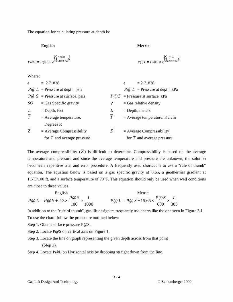
3 - 4Gas Lift Design And Technology Schlumberger 1999
The equation for calculating pressure at depth is:
English Metric
P L P S e
S G L
T Z@ @
. .
.= ××
× ×FHG
IKJ53 34 P L P S e
L
T Z@ @ .= ××× ×
FHG
IKJ
γ29 28
Where:
e = 2.71828 e = 2.71828
P L@ = Pressure at depth, psia P L@ = Pressure at depth, kPa
P S@ = Pressure at surface, psia P S@ = Pressure at surface, kPa
SG = Gas Specific gravity γ = Gas relative density
L = Depth, feet L = Depth, meters
T = Average temperature, T = Average temperature, Kelvin
Degrees R
Z = Average Compressibility Z = Average Compressibility
for T and average pressure for T and average pressure
The average compressibility (Z ) is difficult to determine. Compressibility is based on the average
temperature and pressure and since the average temperature and pressure are unknown, the solution
becomes a repetitive trial and error procedure. A frequently used shortcut is to use a "rule of thumb"
equation. The equation below is based on a gas specific gravity of 0.65, a geothermal gradient at
1.6°F/100 ft. and a surface temperature of 70°F. This equation should only be used when well conditions
are close to these values.
English Metric
P L P SP S L
@ @ .@= + × ×2 3
100 1000P L P S
P S L@ @ .
@= + × ×15 65680 305
In addition to the "rule of thumb", gas lift designers frequently use charts like the one seen in Figure 3.1.
To use the chart, follow the procedure outlined below:
Step 1. Obtain surface pressure P@S.
Step 2. Locate P@S on vertical axis on Figure 1.
Step 3. Locate the line on graph representing the given depth across from that point
(Step 2).
Step 4. Locate P@L on Horizontal axis by dropping straight down from the line.
3 - 7Gas Lift Design And Technology Schlumberger 1999
When the well conditions differ from those given above, pressure at depth is deter-mined using charts
like those seen in Figures 3.2 and 3.3. The following data must be given:
1. Temperature at Surface (T@S) °F [°C]
2. Geothermal Gradient (G/T) °F/100 ft [°C/meter]
3. Specific Gravity (SG.) [Relative Density]
4. Pressure at Surface (P@S) psig [kPa]
5. Depth (L) feet [meters]
The following steps must be completed in order to determine the pressure at a given depth:
Step 1. Determine the temperature at depth by applying the following formula:English: Metric:
T L T STemp Grad L
@ @. .= + ×100
T L T S Temp Grad L@ @ .= + ×
Step 2. Calculate the average temperature:
TT L T S
avg =+@ @b g2
TT L T S
avg =+@ @b g2
Step 3. Estimate the P@L using the "rule of thumb" equation given above.
Step 4. Calculate the average pressure: Pavg = P@L + P@S
PP L P S
avg =+@ @b g2
PP L P S
avg =+@ @b g2
Step 5. Enter Figure 3.2 with the average temperature calculated in Step 2 on the left horizontal axis.
Travel up to the given gas gravity. Travel across the graph to the right.
Step 6. Enter Figure 3.2 with the average pressure estimated in Step 4 and travel upward until the line
intersects the line drawn in Step 5. Read the compressibility factor at the point of intersection.

3 - 8Gas Lift Design And Technology Schlumberger 1999
Step 7. Enter Figure 3.3 with the given gas gravity and travel up to given depth. Travel across to the
average temperature calculated in Step 2. Travel down to the compressibility factor determined
in Step 6. Move across to the surface pressure line (P@S given) and down from this point to the
pressure at depth line. Read the P@L on the lower horizontal axis.
Step 8. Compare P@L with your estimate. If it differs by more than 10%, repeat the entire procedure
using the P@L just determined to calculate the average pressure in Step 4. Repeat the
procedure until the derived P@L becomes constant (at least 2 values for P@L).

3 - 11Gas Lift Design And Technology Schlumberger 1999
VOLUME OF A GAS IN A CONDUIT
It is sometimes necessary to determine the volume of gas in a conduit under given conditions. This is
particularly true when designing conventional and chamber intermitting installations. Equations have
been derived to determine volume in a conduit and determine the gas required to change the pressure
within the conduit.
The internal capacity of a single circular conduit such as a tubing or casing string can be calculated using
the following equations:English Metric
Q (ft3 / 100 ft.) = 0.5454 di2 Q(m3 / 100 meters) = 0.007854 di2
Q (barrels/100 ft.) = 0.009714 di2)
Where:
di = the inside diameter in inches di = the inside diameter in cm
When it is necessary to determine the annular capacity of a tubing string inside casing, the equation
below can be used.
English Metric
Q(ft3 / 100 ft.) = 0.5454 (di2 - do2) Q(m3 / 100 meters = 0.007854(di2 - do2)
Q(barrels/100 ft.) = 0.09714 (di2 - do2)
Where:
di = the inside diameter in inches di = the inside diameter in cmdo = the outside diameter in inches do = the outside diameter in cm
Once the volume or capacity of a conduit has been determined, it is often necessary to find the volume of
gas contained in the conduit under specific well conditions. The equation below can be used for this
purpose:
b VP T
Z P Tb
b
= × ×× ×
Where:
3 - 12Gas Lift Design And Technology Schlumberger 1999
b = gas volume at base conditions
V = capacity of conduit in cubic ft. (see formula above)
P = average pressure within conduit (psia)
Tb = temperature base in degrees Rankin
Z = compressibility factor for average pressure and temperature in a conduit
(See Figure 3.2)
Pb = pressure base (14.73 psi)
T = average temperature in the conduit in degrees Rankin
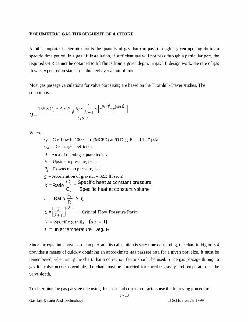
3 - 13Gas Lift Design And Technology Schlumberger 1999
VOLUMETRIC GAS THROUGHPUT OF A CHOKE
Another important determination is the quantity of gas that can pass through a given opening during a
specific time period. In a gas lift installation, if sufficient gas will not pass through a particular port, the
required GLR cannot be obtained to lift fluids from a given depth. In gas lift design work, the rate of gas
flow is expressed in standard cubic feet over a unit of time.
Most gas passage calculations for valve port sizing are based on the Thornhill-Craver studies. The
equation is:
QC A P g
kk
r r
G T
dk k k
=× × × ×
−× −
×
+155 211
2 1/ /a f a f
Where :
Q = Gas flow in 1000 scfd (MCFD) at 60 Deg. F. and 14.7 psia
Cd = Discharge coefficient
A= Area of opening, square inches
P1 = Upstream pressure, psia
P2 = Downstream pressure, psia
g = Acceleration of gravity, = 32.2 ft./sec.2
K = =Ratio C
C
Specific heat at constant pressure
Specific heat at constant volumep
v
r = Ratio P
P r2
1o≥
ro =2
k + 1
k / k−1( )
= Critical Flow Pressure Ratio
G = Specific gravity Air = 1( )T = Inlet temperature, Deg. R.
Since the equation above is so complex and its calculation is very time consuming, the chart in Figure 3.4
provides a means of quickly obtaining an approximate gas passage rata for a given port size. It must be
remembered, when using the chart, that a correction factor should be used. Since gas passage through a
gas lift valve occurs downhole, the chart must be corrected for specific gravity and temperature at the
valve depth.
To determine the gas passage rate using the chart and correction factors use the following procedure:

3 - 14Gas Lift Design And Technology Schlumberger 1999
Step 1. Obtain port size, upstream pressure, downstream pressure, specific gravity (gas gravity), and
temperature in degrees Fahrenheit.
Step 2. Calculate the ratio of downstream pressure to up stream pressure applying the following equation:
RP
Pd
up
=
Step 3. Enter Figure 3.4 with the ratio on the vertical axis.
Step 4. Travel across to the curve and down to the horizontal axis.
Step 5. Read value for K.
Step 6. Read coefficient for port (C) on Figure 3.4.
Step 7. Calculate gas passage Q using the following equation:
Q P K Cup= × ×

3 - 15Gas Lift Design And Technology Schlumberger 1999
Step 8. Correct the chart value by applying the following equation:
English Metric
Qactual =Qchart
.0544 SG × Tf + 460( )Q
Q
l Dens Tactual
chart
f
=× +0 07299 273. Re . ( )
NOTE: "C" in step six is determined by the following equation:
C d= ×46 08 2. C d==== ××××0 29334 2.
Where:
d = port diameter in inches d = port diameter in inches
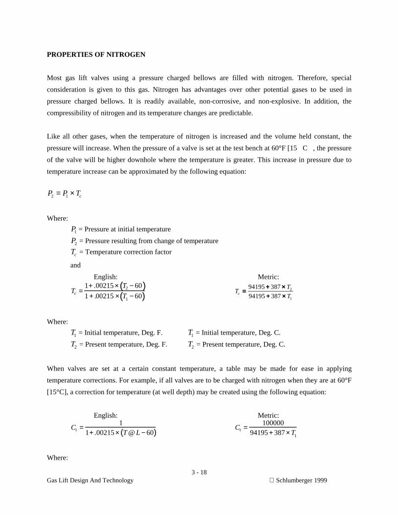
3 - 18Gas Lift Design And Technology Schlumberger 1999
PROPERTIES OF NITROGEN
Most gas lift valves using a pressure charged bellows are filled with nitrogen. Therefore, special
consideration is given to this gas. Nitrogen has advantages over other potential gases to be used in
pressure charged bellows. It is readily available, non-corrosive, and non-explosive. In addition, the
compressibility of nitrogen and its temperature changes are predictable.
Like all other gases, when the temperature of nitrogen is increased and the volume held constant, the
pressure will increase. When the pressure of a valve is set at the test bench at 60°F [15�C�, the pressure
of the valve will be higher downhole where the temperature is greater. This increase in pressure due to
temperature increase can be approximated by the following equation:
P P Tc2 1= ×
Where:
P1 = Pressure at initial temperature
P2 = Pressure resulting from change of temperature
Tc = Temperature correction factor
and
English: Metric:
Tc =1+ .00215× T2 − 60( )1 + .00215 × T1 − 60( ) T
T
Tc ====++++ ××××++++ ××××
94195 387
94195 3872
1
Where:
T1 = Initial temperature, Deg. F. T1 = Initial temperature, Deg. C.
T2 = Present temperature, Deg. F. T2 = Present temperature, Deg. C.
When valves are set at a certain constant temperature, a table may be made for ease in applying
temperature corrections. For example, if all valves are to be charged with nitrogen when they are at 60°F
[15°C], a correction for temperature (at well depth) may be created using the following equation:
English: Metric:
Ct =1
1+ .00215× T @ L − 60( ) Ct =100000
94195+ 387× T1
Where:
3 - 19Gas Lift Design And Technology Schlumberger 1999
Ct = Correction for temperature
T L@ = Temp at valve depth, °F. T L@ = Temp at valve depth, °C.
Then: P C Pb t bt= ×bg
Where:
Pb = Bellows pressure at 60°F., psig Pb = Bellows pressure at 15°C., kPa
Pbt = Bellows pressure at valve depth Pbt = Bellows pressure at valve depth
temp, psig temp, psig
Table 3.1A contains the correction for temperature (Ct) for temperatures from 60°F to 300°F. Table 3.1B
contains the correction for temperature (Ct) for temperatures from 16°C to 150°C. These tables should be
readily available for problems requiring the determination of dome pressure. Since it is based on the most
frequently used pressures and temperatures, it should be limited to use with moderate temperature
corrections. It is not accurate at extreme pressures and temperatures.

3 - 20Gas Lift Design And Technology Schlumberger 1999
TABLE 3.1A
Nitrogen Temperature Correction Factors for Temperature in Fahrenheit
° F Ct ° F Ct ° F Ct ° F Ct ° F Ct ° F °Ct61 0.998 101 0.919 141 0.852 181 0.794 221 0.743 261 0.69862 0.996 102 0.917 142 0.850 182 0.792 222 0.742 262 0.69763 0.994 103 0.915 143 0.849 183 0.791 223 0.740 263 0.69664 0.991 104 0.914 144 0.847 184 0.790 224 0.739 264 0.69565 0.989 105 0.912 145 0.845 185 0.788 225 0.738 265 0.694
66 0.987 106 0.910 146 0.844 186 0.787 226 0.737 266 0.69367 0.985 107 0.908 147 0.842 187 0.786 227 0.736 267 0.69268 0.983 108 0.906 148 0.841 188 0.784 228 0.735 268 0.69169 0.981 109 0.905 149 0.839 189 0.783 229 0.733 269 0.69070 0.979 110 0.903 150 0.838 190 0.782 230 0.732 270 0.689
71 0.977 111 0.901 151 0.836 191 0.780 231 0.731 271 0.68872 0.975 112 0.899 152 0.835 192 0.779 232 0.730 272 0.68773 0.973 113 0.898 153 0.833 193 0.778 233 0.729 273 0.68674 0.971 114 0.896 154 0.832 194 0.776 234 0.728 274 0.68575 0.969 115 0.894 155 0.830 195 0.775 235 0.727 275 0.684
76 0.967 116 0.893 156 0.829 196 0.774 236 0.725 276 0.68377 0.965 117 0.891 157 0.827 197 0.772 237 0.724 277 0.68278 0.963 118 0.889 158 0.826 198 0.771 238 0.723 278 0.68179 0.961 119 0.887 159 0.825 199 0.770 239 0.722 279 0.68080 0.959 120 0.886 160 0.823 200 0.769 240 0.721 280 0.679
81 0.957 121 0.884 161 0.822 201 0.767 241 0.720 281 0.67882 0.955 122 0.882 162 0.820 202 0.766 242 0.719 282 0.67783 0.953 123 0.881 163 0.819 203 0.765 243 0.718 283 0.67684 0.951 124 0.879 164 0.817 204 0.764 244 0.717 284 0.67585 0.949 125 0.877 165 0.816 205 0.762 245 0.715 285 0.674
86 0.947 126 0.876 166 0.814 206 0.761 246 0.714 286 0.67387 0.945 127 0.874 167 0.813 207 0.760 247 0.713 287 0.67288 0.943 128 0.872 168 0.812 208 0.759 248 0.712 288 0.67189 0.941 129 0.871 169 0.810 209 0.757 249 0.711 289 0.67090 0.939 130 0.869 170 0.809 210 0.756 250 0.710 290 0.669
91 0.938 131 0.868 171 0.807 211 0.755 251 0.709 291 0.66892 0.936 132 0.866 172 0.806 212 0.754 252 0.708 292 0.66793 0.934 133 0.864 173 0.805 213 0.752 253 0.707 293 0.66694 0.932 134 0.863 174 0.803 214 0.751 254 0.706 294 0.66595 0.930 135 0.861 175 0.802 215 0.750 255 0.705 295 0.664
96 0.928 136 0.860 176 0.800 216 0.749 256 0.704 296 0.66397 0.926 137 0.858 177 0.799 217 0.748 257 0.702 297 0.66298 0.924 138 0.856 178 0.798 218 0.746 258 0.701 298 0.66299 0.923 139 0.855 179 0.796 219 0.745 259 0.700 299 0.661
100 0.921 140 0.853 180 0.795 220 0.744 260 0.699 300 0.660

3 - 21Gas Lift Design And Technology Schlumberger 1999
TABLE 3.1B
Nitrogen Temperature Correction Factors for Temperature in Celsius
° C Ct ° C Ct ° C Ct ° C Ct16 0.998 51 0.879 86 0.786 121 0.71017 0.994 52 0.876 87 0.783 122 0.70818 0.991 53 0.873 88 0.781 123 0.70619 0.987 54 0.870 89 0.779 124 0.70420 0.983 55 0.868 90 0.776 125 0.702
21 0.979 56 0.865 91 0.774 126 0.70122 0.976 57 0.862 92 0.772 127 0.69923 0.972 58 0.859 93 0.769 128 0.69724 0.968 59 0.856 94 0.767 129 0.69525 0.965 60 0.853 95 0.765 130 0.693
26 0.961 61 0.850 96 0.763 131 0.69127 0.958 62 0.848 97 0.760 132 0.68928 0.954 63 0.845 98 0.758 133 0.68829 0.951 64 0.842 99 0.756 134 0.68630 0.947 65 0.839 100 0.754 135 0.684
31 0.944 66 0.837 101 0.752 136 0.68232 0.940 67 0.834 102 0.749 137 0.68033 0.937 68 0.831 103 0.747 138 0.67834 0.933 69 0.829 104 0.745 139 0.67735 0.930 70 0.826 105 0.743 140 0.675
36 0.927 71 0.823 106 0.741 141 0.67337 0.923 72 0.821 107 0.739 142 0.67138 0.920 73 0.818 108 0.737 143 0.67039 0.917 74 0.816 109 0.734 144 0.66840 0.914 75 0.813 110 0.732 145 0.666
41 0.910 76 0.810 111 0.730 146 0.66542 0.907 77 0.808 112 0.728 147 0.66343 0.904 78 0.805 113 0.726 148 0.66144 0.901 79 0.803 114 0.724 149 0.65945 0.898 80 0.800 115 0.722 150 0.658
46 0.895 81 0.798 116 0.720 151 0.65647 0.892 82 0.795 117 0.718 152 0.65448 0.888 83 0.793 118 0.716 153 0.65349 0.885 84 0.791 119 0.714 154 0.65150 0.882 85 0.788 120 0.712 155 0.649
4-1
Gas Lift Design And Technology Schlumberger 1999
GAS LIFT DESIGN AND TECHNOLOGY
4. Gas Lift Equipment
4-2
Gas Lift Design And Technology Schlumberger 1999
4. Gas Lift Equipment
CHAPTER OBJECTIVE: To get an understanding of the basic gas lift equipment and accessories, with a
more detailed knowledge of gas lift valve mechanics and the application in design and operations.
Introduction
Continuous Gas Lift usually consists of a number of unloading valves with an orifice valve at the operating
point. In this context the role of the unloading gas lift valve should be to allow smooth, positive and reliable
unloading of the well to the orifice over many years with continuously changing conditions. There are
several different types of gas lift valves used in order to achieve this and each uses a particular design
technique. The following is a brief summary of the common types of valve and design techniques used for
continuous gas lift in the North Sea
Injection Pressure Or Casing Pressure Operated Valves
The IPO valves are designed in such a way that the casing pressure is acting on the larger area of the bellows
and thus they are primarily sensitive to the casing pressure (see FIGURE 4-1). The drop in casing pressure
which occurs during unloading is used to close the valves in the correct sequence. The added benefit of this
type of operation is that when the desired injection point is reached then an additional casing pressure drop
can be designed in ensuring the upper valves are firmly closed and that fluctuations in tubing pressure are
very unlikely to result in the valve re-opening. Worldwide they are considered the primary unloading valve
type when continuous gas lifting, being suitable for all conditions other than those in which the PPO valve
excels.
Production Pressure or Tubing Operated Valves
In the PPO valves the flow path is reversed and thus the tubing pressure is acting on the larger area of the
bellows making the valve primarily sensitive to the tubing pressure. The drop in the tubing pressure as gas is
injected is used to close the valve. As this is less predictable than the injection pressure their uses are
generally limited to dual wells where changes in casing pressure would cause interference between the
strings with the IPO valve and also in situations where the injection pressure is prone to fluctuate and the
production pressure can be considered the more predictable.
4-3
Gas Lift Design And Technology Schlumberger 1999
Production Pressure (Tubing) Sensitivity and Gas Passage
The degree to which either type of valve is sensitive to the tubing or casing is determined by the area of the
port in relation to the bellows area i.e. in the Camco R-20 IPO valve the sensitivity to tubing pressure ranges
from 3.8% for a 3/16" port to 26% for the 1/2" port whereas the Camco R-25 PPO valve ranges from 96.2%
for a 3/16" port to 89.7% for the 5/16" port.
As either type of valve acts for the most part like an orifice when fully open then gas passage through the
valve can be calculated accurately using Thornhill Cravers gas passage through a choke corrected for a gas
lift valve using a discharge coefficient. This has been proved to be an accurate method of calculating gas
passage for many years. The large range of port sizes available for these valves enables the design engineer
to size the valve to pass the correct amount of gas for the conditions he would like it to operate under.
Proportional Response Valves
A third type of design has been developed called the Proportional Response Design (PR). This technique is
basically a refined PPO design and utilizes some minor changes to the mechanics of the valve to increase the
throttling range (see FIGURE 4-3). All Gas lift valves have some degree of throttling effect as the ball
approaches the seat and gas passage is restricted i.e. the valve no longer acts as a simple orifice.
If the natural throttling effect of a spring is used (the more you try to compress a spring the greater the force
required) and the seat or port of the valve is beveled or given an angle so that during stem travel (the amount
to which the ball moves off seat as the opening force is increased) the ball never moves out of the flow
stream and thus continues to be sensitive to the tubing pressure then the valve will respond proportionally to
the tubing pressure i.e. the greater the tubing pressure the more the valve will open and thus the more gas the
valve will pass until critical flow is reached.
The result of this is that the valve requires a much larger port to pass gas and this has a considerable impact
on its tubing sensitivity. The LN-21R for example has a tubing sensitivity ranging from 34% for the small
trim up to 60% for the large. Thus while the valve mechanics are basically the same as the IPO valve, the
valve is neither a PPO nor an IPO valve.
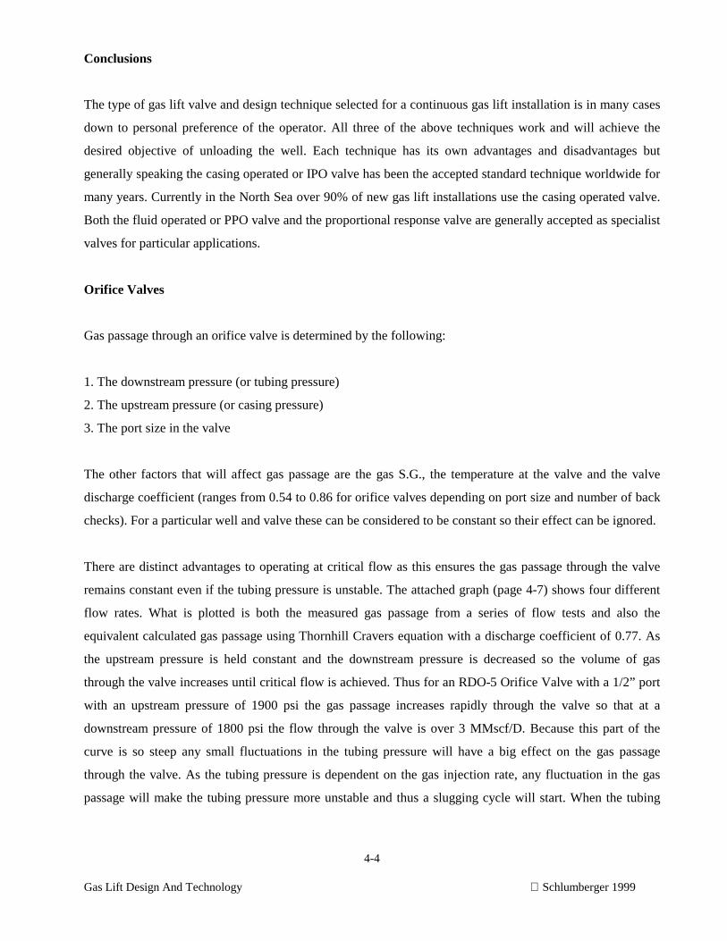
4-4
Gas Lift Design And Technology Schlumberger 1999
Conclusions
The type of gas lift valve and design technique selected for a continuous gas lift installation is in many cases
down to personal preference of the operator. All three of the above techniques work and will achieve the
desired objective of unloading the well. Each technique has its own advantages and disadvantages but
generally speaking the casing operated or IPO valve has been the accepted standard technique worldwide for
many years. Currently in the North Sea over 90% of new gas lift installations use the casing operated valve.
Both the fluid operated or PPO valve and the proportional response valve are generally accepted as specialist
valves for particular applications.
Orifice Valves
Gas passage through an orifice valve is determined by the following:
1. The downstream pressure (or tubing pressure)
2. The upstream pressure (or casing pressure)
3. The port size in the valve
The other factors that will affect gas passage are the gas S.G., the temperature at the valve and the valve
discharge coefficient (ranges from 0.54 to 0.86 for orifice valves depending on port size and number of back
checks). For a particular well and valve these can be considered to be constant so their effect can be ignored.
There are distinct advantages to operating at critical flow as this ensures the gas passage through the valve
remains constant even if the tubing pressure is unstable. The attached graph (page 4-7) shows four different
flow rates. What is plotted is both the measured gas passage from a series of flow tests and also the
equivalent calculated gas passage using Thornhill Cravers equation with a discharge coefficient of 0.77. As
the upstream pressure is held constant and the downstream pressure is decreased so the volume of gas
through the valve increases until critical flow is achieved. Thus for an RDO-5 Orifice Valve with a 1/2” port
with an upstream pressure of 1900 psi the gas passage increases rapidly through the valve so that at a
downstream pressure of 1800 psi the flow through the valve is over 3 MMscf/D. Because this part of the
curve is so steep any small fluctuations in the tubing pressure will have a big effect on the gas passage
through the valve. As the tubing pressure is dependent on the gas injection rate, any fluctuation in the gas
passage will make the tubing pressure more unstable and thus a slugging cycle will start. When the tubing
4-5
Gas Lift Design And Technology Schlumberger 1999
pressure is decreased to 1045 psi (55% of upstream pressure) the valve goes into critical flow at a rate of 7.7
MMscf/D.
In most gas lift applications there is insufficient differential across the valve to operate at critical flow and
hence the benefit of using the NOVA valve. This achieves critical flow at about 90% downstream as opposed
to a square edged orifice which is about 55% downstream pressure. When at critical flow the gas passage
through the valve will be dictated by the upstream pressure only. Thus on the attached graph for the 1/2”
port, the maximum gas passage increases from 4.9 MMscf/D to 7.7 MMscf/D by increasing the casing
pressure from 1200 psi to 1900 psi.
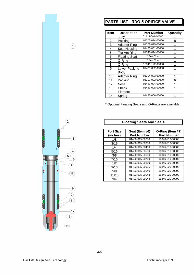
4-6
Gas Lift Design And Technology Schlumberger 1999
PARTS LIST - RDO-5 ORIFICE VALVE
Item Description Part Number Quantity1 Body 01413-001-00000 12 Packing 01302-014-00000 83 Adapter Ring 01302-015-00000 14 Seat Housing 01423-001-00000 15 Tru-Arc Ring 01347-014-00000 16 Floating Seat * See Chart 17 O-Ring * See Chart 18 O-Ring 16846-122-00000 19 Lower Packing
Body01423-002-00000 1
10 Adapter Ring 01304-023-00000 111 Packing 01302-022-00000 612 Nose 01423-004-00000 113 Check
Element01423-008-00000 1
14 Spring 01423-006-00000 1
* Optional Floating Seats and O-Rings are available.
Floating Seats and Seals
Port Size(inches)
Seat (Item #6)Part Number
O-Ring (Item #7)Part Number
1/8 01400-015-00200 16846-210-00000
3/16 01400-015-00300 16846-210-00000
1/4 01400-015-00400 16846-210-00000
5/16 01400-015-00500 16846-210-00000
3/8 01400-015-00600 16846-210-00000
7/16 01400-015-00700 16846-210-00000
1/2 01423-005-00800 16846-020-00000
9/16 01423-005-00036 16846-020-00000
5/8 01423-005-00040 16846-020-00000
11/16 01423-005-00044 16846-020-00000
3/4 01423-005-00048 16846-020-00000
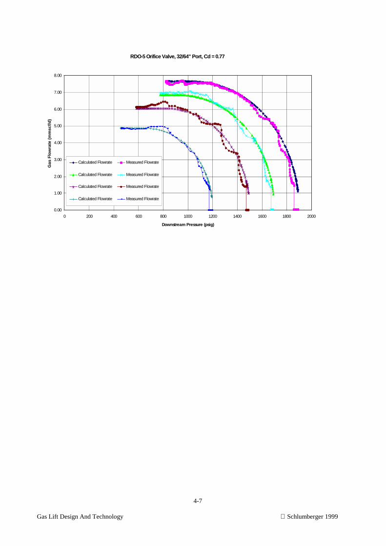
4-7
Gas Lift Design And Technology Schlumberger 1999
RDO-5 Orifice Valve, 32/64" Port, Cd = 0.77
0.00
1.00
2.00
3.00
4.00
5.00
6.00
7.00
8.00
0 200 400 600 800 1000 1200 1400 1600 1800 2000
Downstream Pressure (psig)
Gas
Flo
wra
te (
mm
scf/
d)
Calculated Flowrate Measured Flowrate
Calculated Flowrate Measured Flowrate
Calculated Flowrate Measured Flowrate
Calculated Flowrate Measured Flowrate
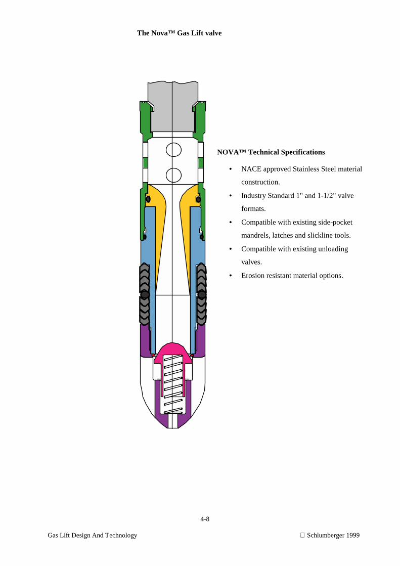
4-8
Gas Lift Design And Technology Schlumberger 1999
The Nova™ Gas Lift valve
NOVA™ Technical Specifications
• NACE approved Stainless Steel material
construction.
• Industry Standard 1" and 1-1/2" valve
formats.
• Compatible with existing side-pocket
mandrels, latches and slickline tools.
• Compatible with existing unloading
valves.
• Erosion resistant material options.
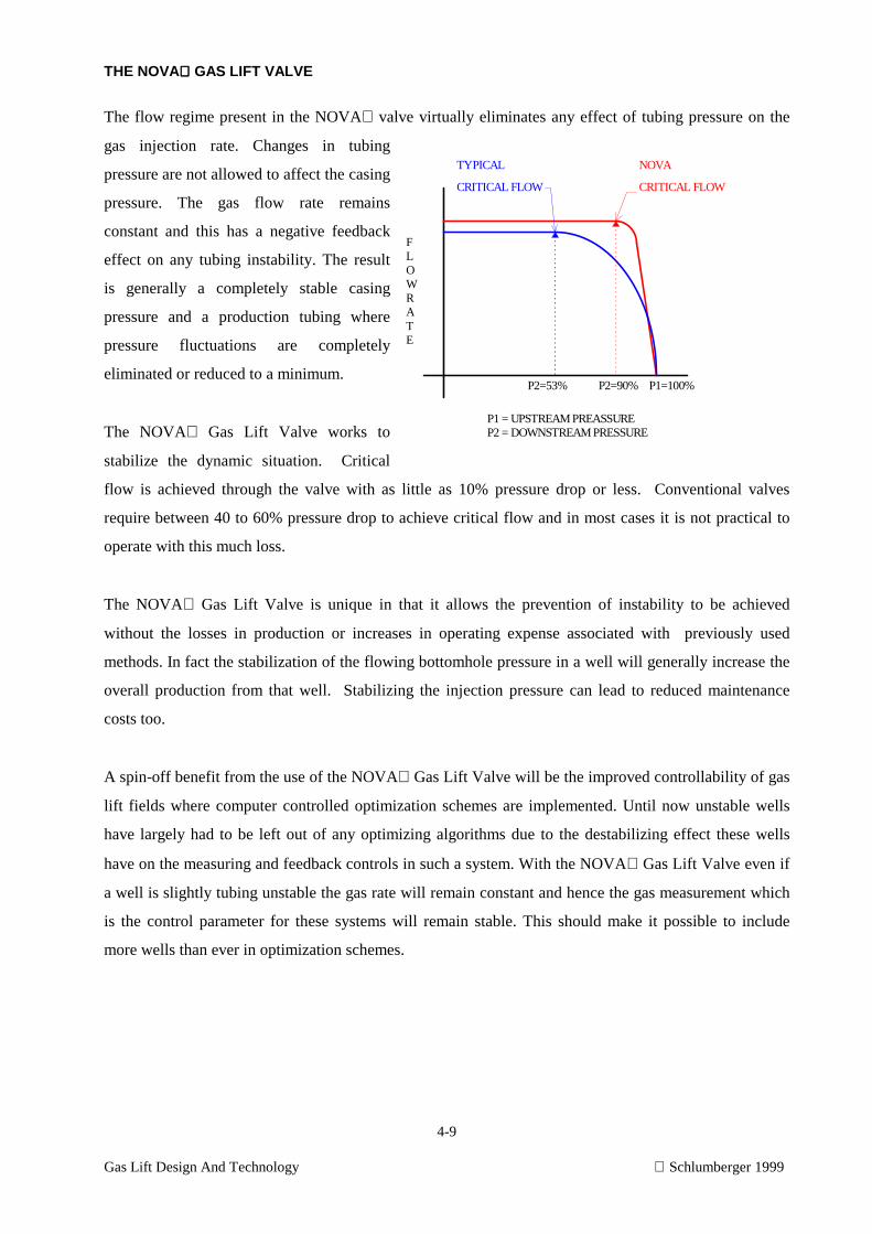
4-9
Gas Lift Design And Technology Schlumberger 1999
THE NOVA GAS LIFT VALVE
The flow regime present in the NOVA valve virtually eliminates any effect of tubing pressure on the
gas injection rate. Changes in tubing
pressure are not allowed to affect the casing
pressure. The gas flow rate remains
constant and this has a negative feedback
effect on any tubing instability. The result
is generally a completely stable casing
pressure and a production tubing where
pressure fluctuations are completely
eliminated or reduced to a minimum.
The NOVA Gas Lift Valve works to
stabilize the dynamic situation. Critical
flow is achieved through the valve with as little as 10% pressure drop or less. Conventional valves
require between 40 to 60% pressure drop to achieve critical flow and in most cases it is not practical to
operate with this much loss.
The NOVA Gas Lift Valve is unique in that it allows the prevention of instability to be achieved
without the losses in production or increases in operating expense associated with previously used
methods. In fact the stabilization of the flowing bottomhole pressure in a well will generally increase the
overall production from that well. Stabilizing the injection pressure can lead to reduced maintenance
costs too.
A spin-off benefit from the use of the NOVA Gas Lift Valve will be the improved controllability of gas
lift fields where computer controlled optimization schemes are implemented. Until now unstable wells
have largely had to be left out of any optimizing algorithms due to the destabilizing effect these wells
have on the measuring and feedback controls in such a system. With the NOVA Gas Lift Valve even if
a well is slightly tubing unstable the gas rate will remain constant and hence the gas measurement which
is the control parameter for these systems will remain stable. This should make it possible to include
more wells than ever in optimization schemes.
P1=100%P2=90%P2=53%
FLOWRATE
TYPICAL NOVA
P1 = UPSTREAM PREASSUREP2 = DOWNSTREAM PRESSURE
CRITICAL FLOW CRITICAL FLOW
4-10
Gas Lift Design And Technology Schlumberger 1999
The Nova Gas Lift Valves and Dual Wells
For many oilfield operators the use of common annulus dual completions (Duals) has been an attractive
way of maximizing the return from a single well drilled into a multi-zone area. The major drawback with
this type of completion has in the past been when attempts have been made to gas lift these wells. The
production tubing in duals have been fed by separate formations which may have similar or widely
different pressure and productivity parameters. However, when gas lifting these duals, only one injection
pressure and surface gas rate is possible which means that both strings must be controlled from the same
gas supply. This has led to sometimes extreme difficulty in maintaining both strings on production, and
often stable production has been impossible. These stability problems have resulted mainly from the fact
that in most cases the flow performance of the downhole gas injection valves has been dependent on the
tubing pressures in the strings as well as the casing pressure common to both strings. This control
problem has usually resulted in one string taking most of the gas injected at surface while the other string
has simply died. One partial solution has been to try to substantially increase the gas flow rate to the
casing in the hope that sufficient pressure would be maintained in the casing to allow gas passage to both
wells. In some cases this would result in the second string functioning again but at the cost of
destabilizing the first string due to excessive gas injection. A technique is required where the
comparative rate of injection of gas to each string is largely independent of the production pressure in the
strings, whether stable or not.
• Analysis of individual strings to optimize gas lift parameters.
• The NOVA Gas Lift Valves for both strings can be set up to pass gas at the appropriate rates based
on a common casing pressure.
• The tubing pressure whether stable or not will no longer affect the gas rate to the strings.
• The casing pressure will stabilize.
• Both strings will act independently of each other and both will be on production simultaneously.
• Over all production rate will increase.
There is more information on the application of the NOVA valve in the instability section, chapter 7.
4-11
Gas Lift Design And Technology Schlumberger 1999
GAS LIFT VALVE CONSTRUCTION AND OPERATION
The advent of the unbalanced single-element bellows-charged gas lift valve revolutionized gas lift
application and design method for lifting oil wells. Prior to the bellows-charged gas lift valve, there were
pressure differential valves and other types of unique devices for gas lifting oil wells. Certain devices, or
valves, were operated by rotating or vertically moving the tubing and by means of a sinker bar on a
slickline.
The original patent for an unbalanced single-element bellows-charged gas lift valve was filed in 1940 by
W.R. King. Today this unbalanced single-element bellows valve remains the most widely used type of
gas lift valve for gas lifting wells. The original King valve had most of the protective design features of
the present gas lift valves. The bellows was protected from high hydrostatic fluid pressure by a gasket
that sealed the bellows chamber from well fluids after full stem travel. A small orifice was drilled in a
bellows guide tube. The orifice was designed to be an anti-chatter mechanism and the bellows guide
provided bellows support.
Unbalanced Single-Element Gas Lift Valves
Single-element implies that the gas lift valve consists of a bellows and dome assembly, stem with a tip
which is usually a carbide ball, and a metal seat housed in a valve body. The unbalanced single-element
gas lift valve is an unbalanced pressure regulator. Unbalanced implies that the pressure applied over the
port area (stem-seat contact area) exerts an opening force; whereas, this same pressure has no effect on
the opening pressure of a balanced backpressure or pressure reducing regulator. The closing force for a
gas lift valve can be a gas pressure charge in the dome and bellow exerted over the effective bellows area
or a spring force or a combination of both a charge pressure and a spring. The closing force for the
regulator or gas lift valve can be adjusted to maintain a desired backpressure for injection pressure
operation or a design downstream pressure for production pressure operation. The regulator or valve will
remain closed until the set closing force is exceeded.
The major initial opening force for most gas lift valves is the pressure exerted over the effective bellows
area less the stem-seat contact area, and the lesser opening force is the pressure acting over the stem-seat
contact area. In like manner for an unbalanced pressure regulator, the major opening pressure is applied
over an area equal to the diaphragm area less the port area. The effect of the unbalanced opening force is
far less for most unbalanced backpressure and pressure reducing regulators than for gas lift valves
because the ratio of the stem-seat contact are to the total effective bellows are of a gas lift valve is much
greater than the ratio of the port area to the total diaphragm area for most regulators. The operating
4-12
Gas Lift Design And Technology Schlumberger 1999
principle is the same for the gas lift valve and regulator, but the pressure applied over the stem-seat
contact area has greater effect on the initial opening pressure of most gas lift valves.
Purposes of Gas Lift and Check Valves
The gas lift valve is considered the heart of most gas lift installations. The predictable performance of
this valve is essential for successful gas lift design and operations. The gas lift valve performs one or
more functions in a typical gas lift installation.
The primary function of the gas lift valves is to unload a well with the available injection gas pressure to
a maximum depth of lift that fully utilizes the energy of expansion of the injection gas pressure from the
depth of gas injection to the surface. Gas lift valves provide the flexibility to permit a changing depth in
the point of gas injection to compensate for a varying flowing bottomhole pressure, water cut, daily
production rate and well deliverability. The operating gas lift valve in an intermittent gas lift installation
prevents an excessive injection gas pressure decrease in the casing annulus following an injection gas
cycle. The operating valve provides the means to control the injection gas volume entering the tubing per
cycle.
Another important function of gas lift valves is the ability to create an excessive flowing bottomhole
pressure drawdown in a temporarily damaged well until the well cleans up. This operation is
accomplished by lifting from near total depth until reservoir deliverability returns to normal. The final
operating depth of gas injection for the stabilized production rate in certain deep wells with a high
reservoir pressure can be nearer the surface than the depth of gas injection to establish initial bottomhole
pressure drawdown during unloading if the load is heavy salt water. Gas lift valves must be installed
below the depth of the operating gas lift valve to create initial bottomhole pressure drawdown and clean
up the well.
When the injection gas line pressure significantly exceeds the flowing bottomhole pressure at the
maximum valve depth, freezing can occur across the surface controls for the injection gas if the operating
valve is a large orifice check valve. The orifice check valve can be replaced by an injection pressure
operated gas lift valve to transfer the pressure drop from the surface to the gas lift valve at well
temperature where hydrates will not form.
The reverse check in a gas lift valve is important for valves below the working fluid level and for testing
the tubing. The check prevents backflow from the tubing to the casing in tubing flow installations. A
reliable check assembly is important if the well produces sand and has a packer to prevent sand from
accumulating in the annulus above the packer.
4-13
Gas Lift Design And Technology Schlumberger 1999
Valve Specifications and Full-Open Stem Travel
Gas lift valve specifications are published by the manufacturers for their valves. Some manufacturers
assume a sharp edged seat for the ball-seat contact area and others arbitrarily add a small incremental
increase to the port ID for a sharp-edged seat to account for a slight bevel at the ball-seat contact. Some
gas lift valve seats have a chamber and the ball or tip on the valve stem contacts the seat on the taper or at
the bottom of the chamber. There is no standard angle of taper or ball-seat size ratio relationship. For
this reason, only sharp-edged seat geometry is used in the installation design calculations in this text.
Since most manufacturers use the same source for their supply of bellows, the effective bellows area for
most 1 and 1-1/2 inch OD valves are relatively standard. The theoretical full-open stem travel is not
included in the typical valve specifications published by most manufacturers. These published gas lift
valve specifications are used primarily in static force balance type equations.
The stem travel required to fully open an unbalanced single-element gas lift valve increases with
increased port size. These curves were calculated for gas lift valves with a sharp-edged ball-seat contact
and a ball on the stem which is 1/16 inch larger in diameter than the bore diameter (ID) of the port. The
equivalent port area before a valve is fully open is based on the lateral area of the frustum of a right
circular cone. The major area of the frustum is the port area which remains constant, and the minor area
decreases with an increase in stem travel as the ball moves away from its ball-seat contact.
There is an important gas lift valve injection gas throughput rate performance consideration that is not
noted in the published literature for most valves. The problem needs to be understood by operators with
high production rate wells being gas lifted through tubing or the casing annulus. An injection gas
throughput rate based on a full-open port size should not be assumed for single-element unbalanced gas
lift valves with large port sizes. For nearly all of these gas lift valves with a large port area relative to the
bellows area, the maximum equivalent port area open to flow of the injection gas will be less than an area
based on the reported port size for an actual range of the surface injection gas pressure during typical
unloading and stabilized gas lift operations. The necessary increase in the injection gas pressure to fully
open a 1 inch OD gas lift valve with a large port can approach or exceed 200 psi. This required stem
travel is not possible for many valves. Maximum stem travel may be limited by a mechanical stop or
bellows stacking before an equivalent full-open port area could be achieved.
4-14
Gas Lift Design And Technology Schlumberger 1999
Bellows Protection
The bellows functions like a piston. A small high pressure diaphragm would not work because of its
limited movement. With a bellows, the travel is distributed uniformly along all the active convolutions
thereby allowing adequate stem travel to obtain the required port opening.
Reputable manufacturers of gas lift valves provide bellows protection in the design of their valves. A
bellows should be protected from a high pressure differential between the bellows-charge and the well
pressures and an unpredictable resonance condition that can result in a high frequency valve stem chatter
and ultimate bellows failure. Gas lift bellows are protected from high hydrostatic well pressures by the
following four methods:-
1) hydraulically performed by a high pressure differential
2) support rings within the convolutions of the bellows
3) confined liquid seal inside or out of a bellows after full steam travel and
4) isolation by a physical seal of the bellows from outside well pressure after full steam
travel
The primary purpose of these methods for protecting the bellows is to prevent a permanent change in the
radii of the convolutions which in turn can effect the operating pressure of a gas lift valve. The highest
pressure differential across a bellows will occur in most installations during initial unloading operations
when the lower gas lift valves are subjected to exceedingly high hydrostatic load fluid pressures in deep
wells. The pressure differential across the bellows of a spring loaded valve will be greater than for a
bellows-charged valve because the dome pressure is atmospheric in spring-loaded valves. The possibility
of a chatter condition is not predictable nor fully understood. The evidence of valve stem chatter will be
a bellows failure and a dished-out seat if the valve seat is not manufactured from an extremely hard
material. Most gas lift valves will have some form of dampening mechanism and the majority of these
devices will operate hydraulically. The bellows will be partially or completely filled with a viscous
liquid to restrict instantaneous undampened stem movement.

4-15
Gas Lift Design And Technology Schlumberger 1999
4-16
Gas Lift Design And Technology Schlumberger 1999
Static Force Balance Equations for Unbalanced Single-Element Bellows-Charged Gas Lift Valves
Most gas lift equipment manufacturers use a valve setting temperature base of 60o for nitrogen charged
gas lift valves. The valve is submerged in a 60oF water bath to ensure a constant nitrogen temperature in
the dome of each valve during the test rack setting procedure. The test rack set initial opening pressure is
measured with the tester pressure applied over the bellows area less the stem-seat contact area with
atmospheric pressure (0 psig) exerted over the stem-seat contact area. For the test rack initial opening
pressure, a valve is actually closed and beginning to open from an opening force that is slightly greater
than the closing force. The tester gas rate through the valve seat is very low. Although most gas lift
valves are set on the basis of an initial opening pressure, test rack closing pressures are used for certain
types of valves with very high production pressure factors and other valves with unique construction.
The test rack closing pressure is determined by slowly bleeding the tester gas from the downstream (port)
side of the gas lift valve after the lift valve has been opened. This theoretical closing pressure occurs
when the downstream and upstream tester pressures are equal at the instant a gas lift valve closes. An
accurate test rack closing pressure is more difficult to observe than a test rack initial opening pressure
and can be affected by the rate of decrease in the tester pressure during bleed-off of the tester gas. An
encapsulating tester with physical capacity for gas in the tester rather than a ring type tester is
recommended for determining accurate test rack closing pressures in order that small leaks in the tester
piping will not prevent observation of the true closing pressure. The tester pressure can be bled-off of
the downstream side of the valve through a small orifice to ensure a more accurate closing pressure
determination.
The equations for initial opening pressure in a tester and well and closing test rack pressure are based on
static force balance equations and apply to unbalanced spring-loaded gas lift valves. The spring pressure
effect replaces the bellows-charge pressure of the valve as the closing force. Several manufacturers of
spring-loaded gas lift valves report a test rack closing pressure for their installation designs. The spring
is adjusted until the force exerted by the spring is equal to the desired test rack closing pressure. Since
there is no nitrogen gas charge pressure in the dome, spring-loaded gas lift valves are not set at a base
tester temperature. Spring-loaded valves are considered temperature insensitive.
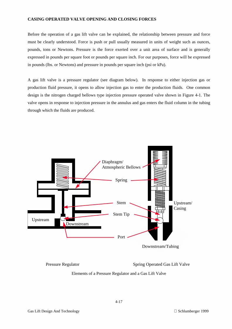
4-17
Gas Lift Design And Technology Schlumberger 1999
CASING OPERATED VALVE OPENING AND CLOSING FORCES
Before the operation of a gas lift valve can be explained, the relationship between pressure and force
must be clearly understood. Force is push or pull usually measured in units of weight such as ounces,
pounds, tons or Newtons. Pressure is the force exerted over a unit area of surface and is generally
expressed in pounds per square foot or pounds per square inch. For our purposes, force will be expressed
in pounds (lbs. or Newtons) and pressure in pounds per square inch (psi or kPa).
A gas lift valve is a pressure regulator (see diagram below). In response to either injection gas or
production fluid pressure, it opens to allow injection gas to enter the production fluids. One common
design is the nitrogen charged bellows type injection pressure operated valve shown in Figure 4-1. The
valve opens in response to injection pressure in the annulus and gas enters the fluid column in the tubing
through which the fluids are produced.
Spring Operated Gas Lift ValvePressure Regulator
Diaphragm/Atmospheric Bellows
Spring
Stem
Stem Tip
Port
DownstreamUpstream
Upstream/Casing
Downstream/Tubing
Elements of a Pressure Regulator and a Gas Lift Valve
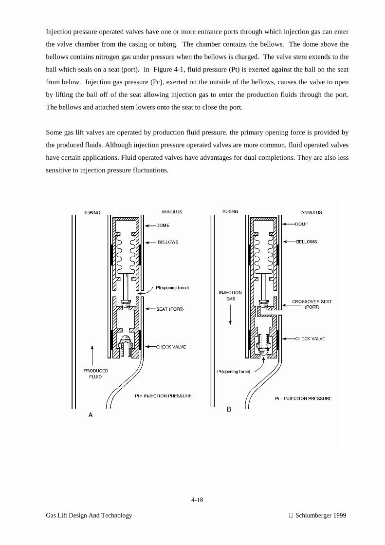
4-18
Gas Lift Design And Technology Schlumberger 1999
Injection pressure operated valves have one or more entrance ports through which injection gas can enter
the valve chamber from the casing or tubing. The chamber contains the bellows. The dome above the
bellows contains nitrogen gas under pressure when the bellows is charged. The valve stem extends to the
ball which seals on a seat (port). In Figure 4-1, fluid pressure (Pt) is exerted against the ball on the seat
from below. Injection gas pressure (Pc), exerted on the outside of the bellows, causes the valve to open
by lifting the ball off of the seat allowing injection gas to enter the production fluids through the port.
The bellows and attached stem lowers onto the seat to close the port.
Some gas lift valves are operated by production fluid pressure. the primary opening force is provided by
the produced fluids. Although injection pressure operated valves are more common, fluid operated valves
have certain applications. Fluid operated valves have advantages for dual completions. They are also less
sensitive to injection pressure fluctuations.
4-19
Gas Lift Design And Technology Schlumberger 1999
The two principal areas of importance for an unbalanced pressure operated valve are the effective area of
the bellows (Ab) and the area of the valve port (Ap). The effective area of the bellows (Ab) is the cross-
sectional area over which a pressure acts. The same force would result if this pressure were exerted on a
piston with a cross-sectional area equal to the effective bellows area. The valve port area (Ap) is equal to
the cross-sectional area of the valve seat.
Closing Force
The closing force for most injection pressure operated gas lift valves is obtained from a pressure charged
bellows (Pb). The bellows functions like a piston. A small high pressure diaphragm would not work
because of its limited movement. With a bellows, the travel is disturbed uniformly along all the active
convolutions thereby allowing adequate stem travel to obtain the required port opening. The closing
force in a nitrogen charged bellows consists of the charge pressure (Pb) exerted over the total effective
bellows area (Ab) and creates a force (Fc) that is applied to the stem. This can be expressed
mathematically as:
Fc = Pb Ab.
Opening Forces
There are two pressures which cause a valve to open, injection or casing pressure (Pc) and production or
tubing pressure (Pt). One opening force (Fo1) is produced by the pressure of the injection gas (Pc)
operating on the effective bellows area (Ab) minus the effective port area (Ap). This first opening force
then, can be expressed mathematically as:
Fo1 = Pc (Ab - Ap)
A second opening force (Fo2) is created by the production pressure (Pt) exerted over the area of the valve
port (Ap) or mathematically as:
Fo2 = Pt Ap
The total opening force (Fo) is the sum of these two forces:
Fo = Fo1 + Fo2
Fo = Pc (Ab - Ap) + Pt Ap
4-20
Gas Lift Design And Technology Schlumberger 1999
Just before the valve opens, the opening force and closing force are equal:
Fo = Fc
Pc (Ab - Ap) + Pt Ap = Pb Ab
Solving for Pc (injection pressure required to balance the opening and closing forces prior to opening an
casing operated valve under operating conditions):
Pb - Pt (Ap / Ab)
Pc = ------------------------------
1 - (Ap / Ab)
Pc Casing pressure.
Pt Tubing pressure.
Ap Area of the portion of the stem tip sealed by the seat (port).
Ab Area of the bellows
Ap/Ab Ratio of port area to bellows area (obtained from valve specifications)
Production Pressure Effect Factor
As discussed earlier, the valve is opened by the forces of Pc acting on the bellows less the area of the
port (Ab-Ap), and Pt acting on the stem tip area that is sealed by the seat. Without Pt to assist opening,
Pc would have to be somewhat greater. The Production Pressure Effect (PPEF) represents the amount
that the opening pressure Pc is reduced as a result of the assistance of Pt.
PPE (sometimes referred to as the tubing effect) is obtained by multiplying production or tubing pressure
(Pt) by the area over which it is applied (Ap) and dividing by the force obtained by the area (Ab - Ap)
over which the valve opening pressure (Pc) acts. The result obtained is the amount the valve opening
pressure (Pc) is reduced in psi:
(Ap / Ab)
PPEF = --------------------
(1 - Ap / Ab)
and is one of the values supplied by valve manufacturers and is found in Table 4.1.
The above equation can, therefore, be expressed as: Pc = Pbt/(1 - Ap/Ab) - Pp x (P.P.E.F.)
Closing Pressure
4-21
Gas Lift Design And Technology Schlumberger 1999
The closing pressure of the valve will be equal to the injection gas opening pressure (Pc) if the
production pressure remains constant. The minimum closing pressure is equal to the dome pressure (Pb)
only at the time when the production, injection and dome pressure are equal.
To solve for production pressure when casing pressure and bellows charge pressure are known, the
following operations must be performed. First, solve for Pt x (Ap/Ab) by transposing this value with Pbt
and making all appropriate sign changes to yield:
Pp x (Ap/Ab) = Pbt - Pc x (1 - Ap/Ab)
Then the equation above is divided by (Ap/Ab) to yield:
Pp = Pb / (Ap/Ab) - [Pc x (1 - Ap/Ab) / (Ap/Ab)]
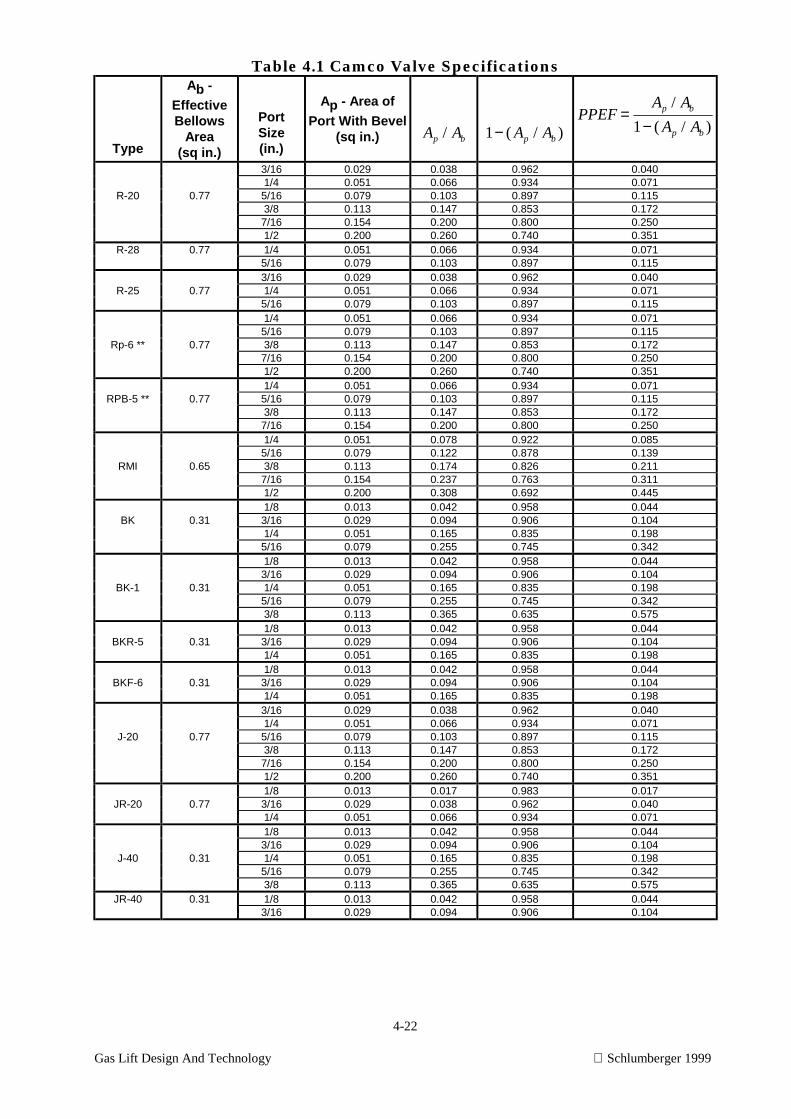
4-22
Gas Lift Design And Technology Schlumberger 1999
Table 4.1 Camco Valve Specifications
Type
Ab -
EffectiveBellows
Area(sq in.)
PortSize(in.)
Ap - Area of
Port With Bevel(sq in.) A Ap b/ 1− ( / )A Ap b
PPEFA A
A Ap b
p b
=−
/
( / )1
3/16 0.029 0.038 0.962 0.0401/4 0.051 0.066 0.934 0.071
R-20 0.77 5/16 0.079 0.103 0.897 0.1153/8 0.113 0.147 0.853 0.1727/16 0.154 0.200 0.800 0.2501/2 0.200 0.260 0.740 0.351
R-28 0.77 1/4 0.051 0.066 0.934 0.0715/16 0.079 0.103 0.897 0.1153/16 0.029 0.038 0.962 0.040
R-25 0.77 1/4 0.051 0.066 0.934 0.0715/16 0.079 0.103 0.897 0.1151/4 0.051 0.066 0.934 0.0715/16 0.079 0.103 0.897 0.115
Rp-6 ** 0.77 3/8 0.113 0.147 0.853 0.1727/16 0.154 0.200 0.800 0.2501/2 0.200 0.260 0.740 0.3511/4 0.051 0.066 0.934 0.071
RPB-5 ** 0.77 5/16 0.079 0.103 0.897 0.1153/8 0.113 0.147 0.853 0.1727/16 0.154 0.200 0.800 0.2501/4 0.051 0.078 0.922 0.0855/16 0.079 0.122 0.878 0.139
RMI 0.65 3/8 0.113 0.174 0.826 0.2117/16 0.154 0.237 0.763 0.3111/2 0.200 0.308 0.692 0.4451/8 0.013 0.042 0.958 0.044
BK 0.31 3/16 0.029 0.094 0.906 0.1041/4 0.051 0.165 0.835 0.1985/16 0.079 0.255 0.745 0.3421/8 0.013 0.042 0.958 0.0443/16 0.029 0.094 0.906 0.104
BK-1 0.31 1/4 0.051 0.165 0.835 0.1985/16 0.079 0.255 0.745 0.3423/8 0.113 0.365 0.635 0.5751/8 0.013 0.042 0.958 0.044
BKR-5 0.31 3/16 0.029 0.094 0.906 0.1041/4 0.051 0.165 0.835 0.1981/8 0.013 0.042 0.958 0.044
BKF-6 0.31 3/16 0.029 0.094 0.906 0.1041/4 0.051 0.165 0.835 0.1983/16 0.029 0.038 0.962 0.0401/4 0.051 0.066 0.934 0.071
J-20 0.77 5/16 0.079 0.103 0.897 0.1153/8 0.113 0.147 0.853 0.1727/16 0.154 0.200 0.800 0.2501/2 0.200 0.260 0.740 0.3511/8 0.013 0.017 0.983 0.017
JR-20 0.77 3/16 0.029 0.038 0.962 0.0401/4 0.051 0.066 0.934 0.0711/8 0.013 0.042 0.958 0.0443/16 0.029 0.094 0.906 0.104
J-40 0.31 1/4 0.051 0.165 0.835 0.1985/16 0.079 0.255 0.745 0.3423/8 0.113 0.365 0.635 0.575
JR-40 0.31 1/8 0.013 0.042 0.958 0.0443/16 0.029 0.094 0.906 0.104
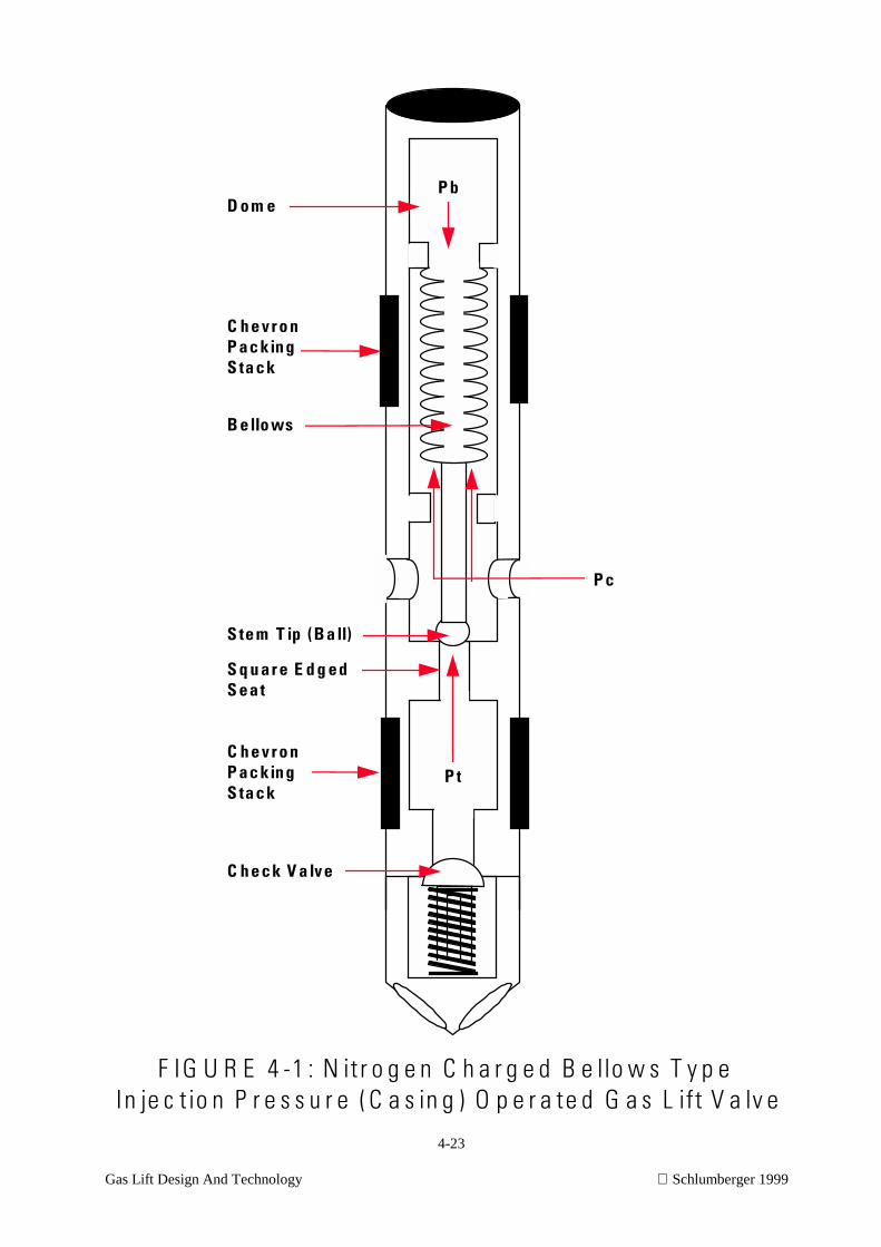
4-23
Gas Lift Design And Technology Schlumberger 1999
P t
P c
P bD o m e
B ello ws
S q u ar e E d g edS ea t
C h e ck V a lv e
C h e v r o n P ac kin gS ta ck
F IG U R E 4 -1 : N it r o g e n C h a r g e d B e llo w s T y p e In je c t io n P r e s s u r e ( C a s in g ) O p e r a te d G a s L ift V a lv e
C h e v r o n P ac kin gS ta ck
S te m T ip (B a ll)
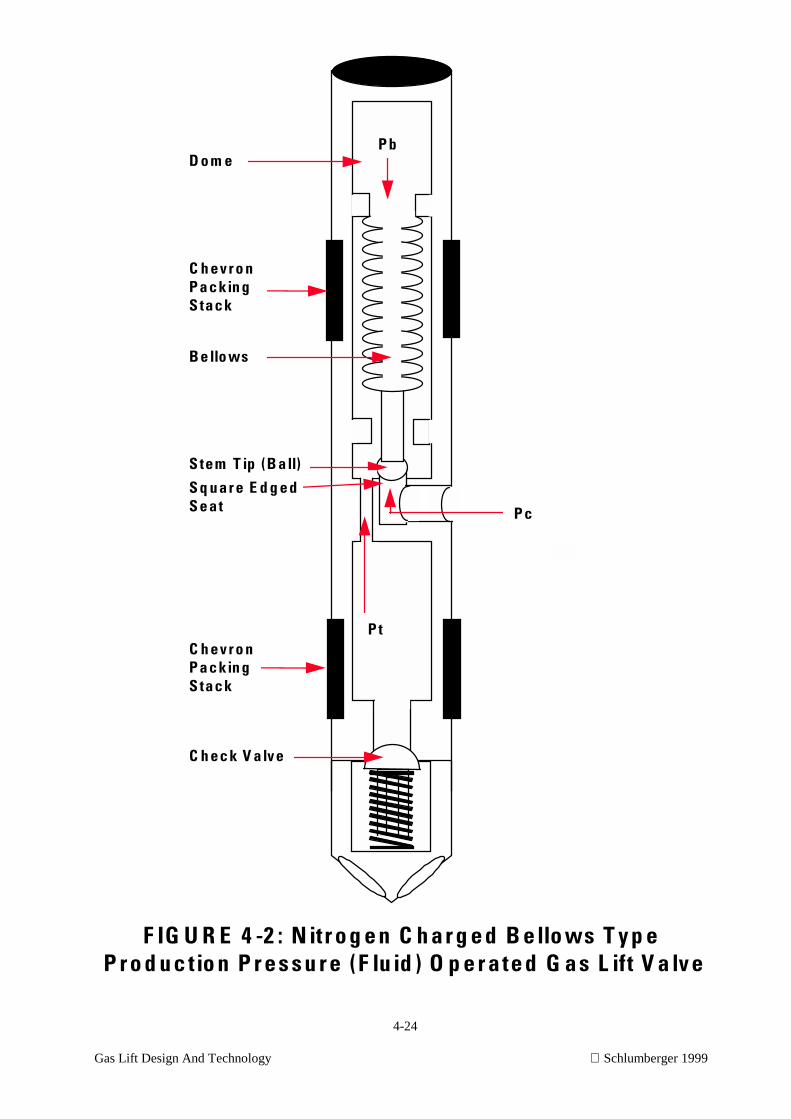
4-24
Gas Lift Design And Technology Schlumberger 1999
P t
P c
P bD o m e
B e llo ws
C h ec k V alv e
C h ev r o n P a ckin gS tack
F IG U R E 4 -2 : N itr o g e n C h ar g e d B ello ws T y p e P r o d u c tio n P r es s u r e (F lu id ) O p e r a te d G a s L ift V a lv e
C h ev r o n P a ckin gS tack
S tem T ip (B all)
S q u ar e E d g e dS e at
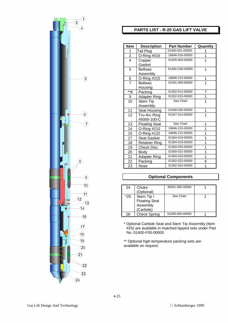
4-25
Gas Lift Design And Technology Schlumberger 1999
PARTS LIST - R-20 GAS LIFT VALVE
Item Description Part Number Quantity1 Tail Plug 01400-001-00000 12 O-Ring #016 16846-016-00000 14 Copper
Gasket01400-003-00000 1
5 BellowsAssembly
01400-C00-00000 1
6 O-Ring #215 16846-215-00000 17 Bellows
Housing01401-009-00000 1
**8 Packing 01302-014-00000 79 Adapter Ring 01302-015-00000 110 Stem Tip
AssemblySee Chart 1
11 Seat Housing 01400-030-00000 112 Tru-Arc Ring
#5000-100-C01347-014-00000 1
13 Floating Seat See Chart 114 O-Ring #210 16846-210-00000 115 O-Ring #122 16846-122-00000 117 Seat Gasket 01304-018-00000 118 Retainer Ring 01304-019-00000 119 Check Disc 01304-020-00000 120 Body 01400-021-00000 121 Adapter Ring 01304-023-00000 122 Packing 01302-022-00000 623 Nose 01302-024-00000 1
Optional Components
24 Choke(Optional)
40001-005-00000 1
*25 Stem Tip /Floating SeatAssembly(Carbide)
See Chart 1
26 Check Spring 01400-005-00000 1
* Optional Carbide Seat and Stem Tip Assembly (Item#25) are available in matched lapped sets under PartNo. 01400-F00-00000.
** Optional high-temperature packing sets areavailable on request.
4-26
Gas Lift Design And Technology Schlumberger 1999
The bellows charge pressure Pbt would exist in a valve operating downhole. Since the valves are set at
the surface at a different temperature (60° F) [15° C] all bellows charge pressures must be converted to
pressure at standard condition (Pb).
The first step is to convert the pressure using the temperature correction factor (Ct) found in Table 4.2.
The following operation corrects the pressure to test bench conditions.
Pb = Ct x (Pbt)
The pressure setting on the test bench at 60° F [15° C] or Test Rack Opening pressure (TRO) can be
determined by dividing the corrected pressure by (1 - Ap/Ab) to produce:
TRO = Pb / (1 - Ap/Ab)
For those valves whose primary opening pressure comes from the production fluids, a special crossover
seat allows production fluid to enter the valve chamber and act upon the effective area of the bellows. As
we saw in the injection pressure operated valves, there is only one closing force and that is the bellows
charge pressure times the effective area of the bellows (Pbt x Ab). The two opening forces have been
reversed since the production fluid replaces the injection gas as the principle opening force Pp x (Ab -
Ap). The injection gas pressure acts to create the second opening force by acting upon the area of the
valve port Pi x (Av). The resulting force balance equation is:
Pbt x (Ab) = Pp x (Ab - Ap) + Pc x (Ap)
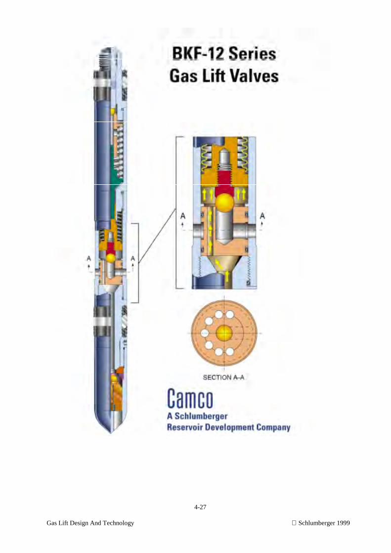
4-27
Gas Lift Design And Technology Schlumberger 1999
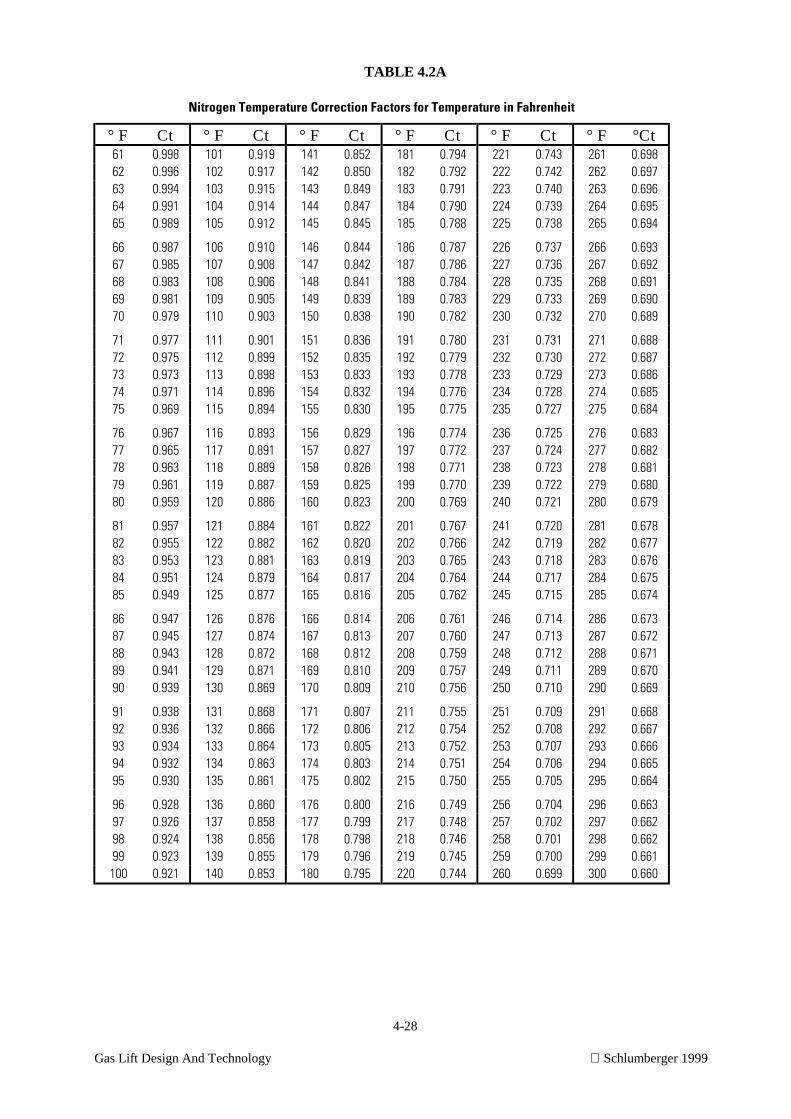
4-28
Gas Lift Design And Technology Schlumberger 1999
TABLE 4.2A
Nitrogen Temperature Correction Factors for Temperature in Fahrenheit
° F Ct ° F Ct ° F Ct ° F Ct ° F Ct ° F °Ct61 0.998 101 0.919 141 0.852 181 0.794 221 0.743 261 0.69862 0.996 102 0.917 142 0.850 182 0.792 222 0.742 262 0.69763 0.994 103 0.915 143 0.849 183 0.791 223 0.740 263 0.69664 0.991 104 0.914 144 0.847 184 0.790 224 0.739 264 0.69565 0.989 105 0.912 145 0.845 185 0.788 225 0.738 265 0.694
66 0.987 106 0.910 146 0.844 186 0.787 226 0.737 266 0.69367 0.985 107 0.908 147 0.842 187 0.786 227 0.736 267 0.69268 0.983 108 0.906 148 0.841 188 0.784 228 0.735 268 0.69169 0.981 109 0.905 149 0.839 189 0.783 229 0.733 269 0.69070 0.979 110 0.903 150 0.838 190 0.782 230 0.732 270 0.689
71 0.977 111 0.901 151 0.836 191 0.780 231 0.731 271 0.68872 0.975 112 0.899 152 0.835 192 0.779 232 0.730 272 0.68773 0.973 113 0.898 153 0.833 193 0.778 233 0.729 273 0.68674 0.971 114 0.896 154 0.832 194 0.776 234 0.728 274 0.68575 0.969 115 0.894 155 0.830 195 0.775 235 0.727 275 0.684
76 0.967 116 0.893 156 0.829 196 0.774 236 0.725 276 0.68377 0.965 117 0.891 157 0.827 197 0.772 237 0.724 277 0.68278 0.963 118 0.889 158 0.826 198 0.771 238 0.723 278 0.68179 0.961 119 0.887 159 0.825 199 0.770 239 0.722 279 0.68080 0.959 120 0.886 160 0.823 200 0.769 240 0.721 280 0.679
81 0.957 121 0.884 161 0.822 201 0.767 241 0.720 281 0.67882 0.955 122 0.882 162 0.820 202 0.766 242 0.719 282 0.67783 0.953 123 0.881 163 0.819 203 0.765 243 0.718 283 0.67684 0.951 124 0.879 164 0.817 204 0.764 244 0.717 284 0.67585 0.949 125 0.877 165 0.816 205 0.762 245 0.715 285 0.674
86 0.947 126 0.876 166 0.814 206 0.761 246 0.714 286 0.67387 0.945 127 0.874 167 0.813 207 0.760 247 0.713 287 0.67288 0.943 128 0.872 168 0.812 208 0.759 248 0.712 288 0.67189 0.941 129 0.871 169 0.810 209 0.757 249 0.711 289 0.67090 0.939 130 0.869 170 0.809 210 0.756 250 0.710 290 0.669
91 0.938 131 0.868 171 0.807 211 0.755 251 0.709 291 0.66892 0.936 132 0.866 172 0.806 212 0.754 252 0.708 292 0.66793 0.934 133 0.864 173 0.805 213 0.752 253 0.707 293 0.66694 0.932 134 0.863 174 0.803 214 0.751 254 0.706 294 0.66595 0.930 135 0.861 175 0.802 215 0.750 255 0.705 295 0.664
96 0.928 136 0.860 176 0.800 216 0.749 256 0.704 296 0.66397 0.926 137 0.858 177 0.799 217 0.748 257 0.702 297 0.66298 0.924 138 0.856 178 0.798 218 0.746 258 0.701 298 0.66299 0.923 139 0.855 179 0.796 219 0.745 259 0.700 299 0.661100 0.921 140 0.853 180 0.795 220 0.744 260 0.699 300 0.660
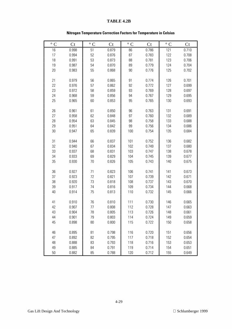
4-29
Gas Lift Design And Technology Schlumberger 1999
TABLE 4.2B
Nitrogen Temperature Correction Factors for Temperature in Celsius
° C Ct ° C Ct ° C Ct ° C Ct16 0.998 51 0.879 86 0.786 121 0.71017 0.994 52 0.876 87 0.783 122 0.70818 0.991 53 0.873 88 0.781 123 0.70619 0.987 54 0.870 89 0.779 124 0.70420 0.983 55 0.868 90 0.776 125 0.702
21 0.979 56 0.865 91 0.774 126 0.70122 0.976 57 0.862 92 0.772 127 0.69923 0.972 58 0.859 93 0.769 128 0.69724 0.968 59 0.856 94 0.767 129 0.69525 0.965 60 0.853 95 0.765 130 0.693
26 0.961 61 0.850 96 0.763 131 0.69127 0.958 62 0.848 97 0.760 132 0.68928 0.954 63 0.845 98 0.758 133 0.68829 0.951 64 0.842 99 0.756 134 0.68630 0.947 65 0.839 100 0.754 135 0.684
31 0.944 66 0.837 101 0.752 136 0.68232 0.940 67 0.834 102 0.749 137 0.68033 0.937 68 0.831 103 0.747 138 0.67834 0.933 69 0.829 104 0.745 139 0.67735 0.930 70 0.826 105 0.743 140 0.675
36 0.927 71 0.823 106 0.741 141 0.67337 0.923 72 0.821 107 0.739 142 0.67138 0.920 73 0.818 108 0.737 143 0.67039 0.917 74 0.816 109 0.734 144 0.66840 0.914 75 0.813 110 0.732 145 0.666
41 0.910 76 0.810 111 0.730 146 0.66542 0.907 77 0.808 112 0.728 147 0.66343 0.904 78 0.805 113 0.726 148 0.66144 0.901 79 0.803 114 0.724 149 0.65945 0.898 80 0.800 115 0.722 150 0.658
46 0.895 81 0.798 116 0.720 151 0.65647 0.892 82 0.795 117 0.718 152 0.65448 0.888 83 0.793 118 0.716 153 0.65349 0.885 84 0.791 119 0.714 154 0.65150 0.882 85 0.788 120 0.712 155 0.649
4-30
Gas Lift Design And Technology Schlumberger 1999
Frequently, production pressure operated valves use a spring to supply the closing forces as illustrated in
Figure below. This valves have an uncharged (14.7 psig) [101.32 kPa] bellows. In the force balance
equation, the spring pressure effect (Pst) is used in stead of the bellows charge pressure at well
temperature (Pbt). The force balance equation for these valves must include one additional value. Unlike
pressure charged valves, the load rate of the valve bellows should be included in the calculation of the
valve's opening pressure in a well. Load rate is a measure of the force required to compress or stretch the
bellows in a gas lift valve at its opening pressure. The measure of bellows load rate used for a gas lift
valve is the increase in pressure required to obtain a given stem travel (psi/in.) [kPa/mm] rather than the
units of force (lbs.)
To account for a valve's bellows load rate and insure adequate gas through-put, the valve's opening
pressure should be set lower than calculated with the above force balance equations. One design
technique used is to ignore the forces exerted by the injection pressure applied over the port area so that
the force balance equation is:
Pst = Pp x (1 - Ap/Ab)
Another "rule of thumb", which is particularly applicable to the higher load rate of the spring loaded
valve, is to subtract an arbitrary pressure difference (Pk) from the production pressure to yield the
following force balance equation:
Pst = (Pp - Pk) x (1 - Ap/Ab) + Pc x (Ap/Ab)
The value of Pk is a least 60 psi. [400 kPa] As a "rule of thumb", 60 psi [400 kPa] is used for 1-1/2"
valves and 75 psi [500 kPa] is used for 1" valves.
The tester for tubing pressure operated valve is designed to apply the opening pressure over the effective
bellows less the port in the same manner employed for a casing pressure operated valve
The equation below is for Test Rack Opening pressure for spring loaded valves:
TRO = Pst / (1 - Ap /.Ab)
No temperature correction is required for the spring loaded valve.

4-31
Gas Lift Design And Technology Schlumberger 1999
4-32
Gas Lift Design And Technology Schlumberger 1999
When a valve is placed in a bench tester only atmospheric pressure is applied over the small port area as
production pressure below the seat. The nitrogen pressure applied externally to the area of bellows less
seat area is used to cause the valve to open in order to set it. When the nitrogen pressure is shut off using
the needle valve on the test rack, the set pressure is "locked" in the bellows chamber (not the bellows)
because the ball is on the seat. In reality, a small amount of leakage from the valve is typical.
In order to determine why a small leak is expected, we can calculate the forces trying to open and close
the valve to find out what the force of the ball against the seat is at the time the valve closes in the tester.
First, let's assume the valve is set to 800 psi [5515 kPa]. This means that when we apply that pressure
from our supply on the test bench, the valve will begin to open and we can hear nitrogen escaping
through the nose of the valve. This means that we must have a lower pressure in the dome of the valve in
order to offset the effect of the seat area. If the bellows is a 0.31 sq. in. [1.99 sq. cm.] and the port is 0.25
inch [0.635 cm.] diameter, the area that the pressure is acting upon is 0.2609 sq. in. [0.6627 sq. cm.] and
the pressure in the bellows is acting over the full 0.31 sq. in. [0.7874 sq. cm.]. The ratio of these two
areas is approximately 0.8416, so the pressure in the bellows must be only 84.16% of the applied
pressure. This calculates to 674 psi [4649 kPa]. Under these conditions, the force of the ball against the
seat is 0 pounds [0 kg].
When we close the needle valve on the tester, the pressure is supposed to be trapped in the valve because
the ball is on the seat. It is true that the ball is on the seat, but at this moment the closing forces (pressure
in the bellows times the bellows area) are equal to the opening forces (the pressure trapped in the valve
outside of the bellows times the bellows area minus the area of the port). The net force (closing force
minus opening force) holding the ball against the seat is virtually nil. As a result of this fact, it is not
unusual to experience some leakage from the valve until the trapped pressure in the valve has dropped
sufficiently to create enough net closing force to effect a seal. Usually a drop of 50 psi [345 kPa] is
sufficient to accomplish this.
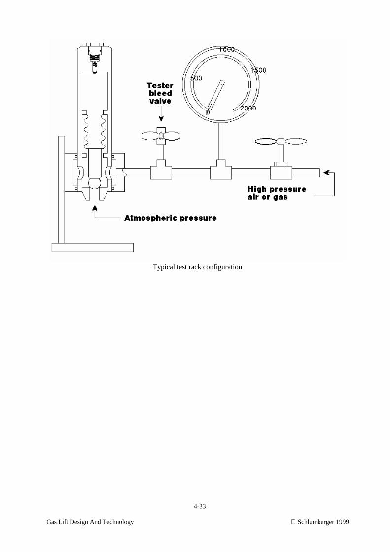
4-33
Gas Lift Design And Technology Schlumberger 1999
Typical test rack configuration
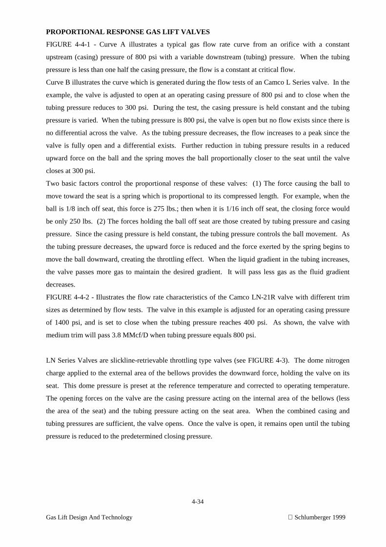
4-34
Gas Lift Design And Technology Schlumberger 1999
PROPORTIONAL RESPONSE GAS LIFT VALVES
FIGURE 4-4-1 - Curve A illustrates a typical gas flow rate curve from an orifice with a constant
upstream (casing) pressure of 800 psi with a variable downstream (tubing) pressure. When the tubing
pressure is less than one half the casing pressure, the flow is a constant at critical flow.
Curve B illustrates the curve which is generated during the flow tests of an Camco L Series valve. In the
example, the valve is adjusted to open at an operating casing pressure of 800 psi and to close when the
tubing pressure reduces to 300 psi. During the test, the casing pressure is held constant and the tubing
pressure is varied. When the tubing pressure is 800 psi, the valve is open but no flow exists since there is
no differential across the valve. As the tubing pressure decreases, the flow increases to a peak since the
valve is fully open and a differential exists. Further reduction in tubing pressure results in a reduced
upward force on the ball and the spring moves the ball proportionally closer to the seat until the valve
closes at 300 psi.
Two basic factors control the proportional response of these valves: (1) The force causing the ball to
move toward the seat is a spring which is proportional to its compressed length. For example, when the
ball is 1/8 inch off seat, this force is 275 lbs.; then when it is 1/16 inch off seat, the closing force would
be only 250 lbs. (2) The forces holding the ball off seat are those created by tubing pressure and casing
pressure. Since the casing pressure is held constant, the tubing pressure controls the ball movement. As
the tubing pressure decreases, the upward force is reduced and the force exerted by the spring begins to
move the ball downward, creating the throttling effect. When the liquid gradient in the tubing increases,
the valve passes more gas to maintain the desired gradient. It will pass less gas as the fluid gradient
decreases.
FIGURE 4-4-2 - Illustrates the flow rate characteristics of the Camco LN-21R valve with different trim
sizes as determined by flow tests. The valve in this example is adjusted for an operating casing pressure
of 1400 psi, and is set to close when the tubing pressure reaches 400 psi. As shown, the valve with
medium trim will pass 3.8 MMcf/D when tubing pressure equals 800 psi.
LN Series Valves are slickline-retrievable throttling type valves (see FIGURE 4-3). The dome nitrogen
charge applied to the external area of the bellows provides the downward force, holding the valve on its
seat. This dome pressure is preset at the reference temperature and corrected to operating temperature.
The opening forces on the valve are the casing pressure acting on the internal area of the bellows (less
the area of the seat) and the tubing pressure acting on the seat area. When the combined casing and
tubing pressures are sufficient, the valve opens. Once the valve is open, it remains open until the tubing
pressure is reduced to the predetermined closing pressure.
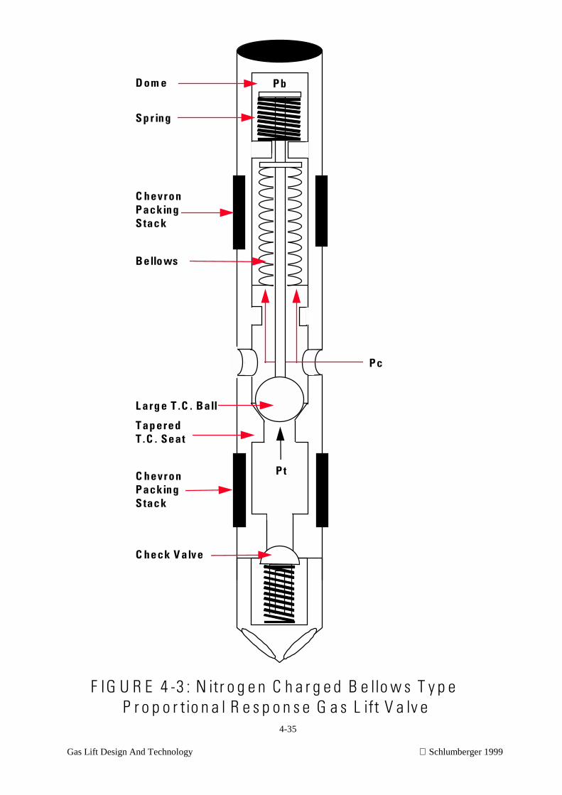
4-35
Gas Lift Design And Technology Schlumberger 1999
P t
P c
P bD om e
Bellows
T ap eredT .C . Seat
C heck V alve
C hevron P ackingS tack
F IG U R E 4 -3 : N itr o g e n C h a r g e d B e llo w s T y p e P r o p o r tio n a l R e s p o n s e G a s L ift V a lv e
C hevron P ackingS tack
S p r ing
L arg e T .C . Ball
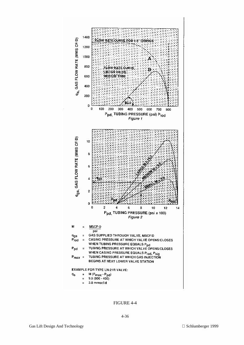
4-36
Gas Lift Design And Technology Schlumberger 1999
FIGURE 4-4
4-37
Gas Lift Design And Technology Schlumberger 1999
CAMCO SIDEPOCKET MANDRELS
Introduction
Camco's introduction of the sidepocket mandrel in 1954 revolutionized the world of gas lift and
completion technology by providing a more flexible, efficient alternative to conventional mandrels. Since
1954, Camco has continually improved and refined the sidepocket mandrel design to provide customers
with the most technologically advanced mandrels for a variety of applications.
Camco's KBG and MMRG round series sidepocket mandrels are made up as part of the tubing string
when preparing a well for gas lift production, chemical injection, or other special applications. The
mandrel can be located anywhere in the tubing string between the annular safety valve and the packer.
The KBG and MMRG sidepocket mandrel is available in various tubing sizes and reduced O.D. sizes.
Each KBG and MMRG series mandrel has eccentric swages on both ends and a "machined" type solid
sidepocket. This sidepocket serves as a receiver for 1” or 1-1/2" dummy and gas lift valves.
Description
The mandrel pocket consists of a latch lug and two polished bore packing sections straddling holes which
provide communication between the casing annulus and the tubing. Each slickline retrievable gas lift
valve has packing which seals in the polished bore sections, above and below the casing ports in the
mandrel pocket. The packing prevents leakage and ensures direct communication between the annulus
and the valve once the valve is secured in the mandrel pocket.
The KBG and MMRG series sidepocket mandrel incorporates additional design features which are
designated by the letter "G". These features include a guide or "orienting sleeve" for aligning sidepocket
accessories by receiving the "finger" on the OK or OM kickover tool and positively orienting the tool
with the pocket. This feature allows ease of installation and retrieval of gas lift valves even in high
deviations of up to 700.
A machined tool discriminator above the mandrel pocket guides the smaller sidepocket equipment into
the pocket, and automatically deflects larger diameter tools into the tubing bore. The latch recess in this
series of mandrel is the 'G' style profile. This takes a BK-2 style latch in the KBG series or an RK Latch
in the MMRG series.

4-38
Gas Lift Design And Technology Schlumberger 1999

4-39
Gas Lift Design And Technology Schlumberger 1999
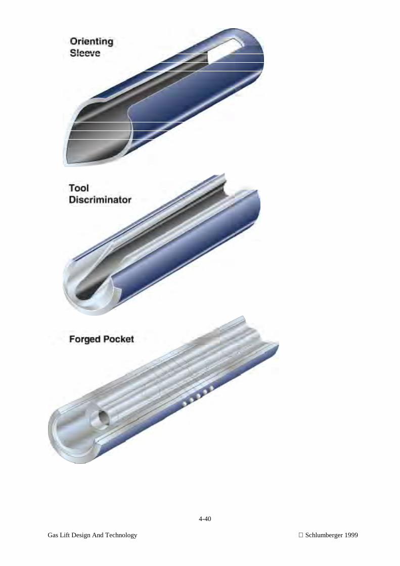
4-40
Gas Lift Design And Technology Schlumberger 1999
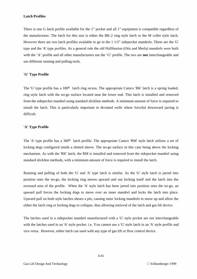
4-41
Gas Lift Design And Technology Schlumberger 1999
Latch Profiles
There is one G latch profile available for the 1” pocket and all 1” equipment is compatible regardless of
the manufacturer. The latch for this size is either the BK-2 ring style latch or the M collet style latch.
However there are two latch profiles available to go in the 1 1/2” sidepocket mandrels. These are the 'G'
type and the 'A' type profiles. As a general rule the old Halliburton (Otis and Merla) mandrels were built
with the ‘A’ profile and all other manufacturers use the ‘G’ profile. The two are not interchangeable and
use different running and pulling tools.
'G' Type Profile
The 'G' type profile has a 180o latch ring recess. The appropriate Camco 'RK' latch is a spring loaded,
ring style latch with the no-go surface located near the lower end. This latch is installed and removed
from the sidepocket mandrel using standard slickline methods. A minimum amount of force is required to
install the latch. This is particularly important in deviated wells where forceful downward jarring is
difficult.
'A' Type Profile
The 'A' type profile has a 360o latch profile. The appropriate Camco 'RM' style latch utilizes a set of
locking dogs configured inside a slotted sleeve. The no-go surface in this case being above the locking
mechanism. As with the 'RK' latch, the RM is installed and removed from the sidepocket mandrel using
standard slickline methods, with a minimum amount of force is required to install the latch.
Running and pulling of both the 'G' and 'A' type latch is similar. As the 'G' style latch is jarred into
position onto the no-go, the locking ring moves upward and out locking itself and the latch into the
recessed area of the profile. When the 'A' style latch has been jarred into position onto the no-go, an
upward pull forces the locking dogs to move over an inner mandrel and locks the latch into place.
Upward pull on both style latches shears a pin, causing inner locking mandrels to move up and allow the
either the latch ring or locking dogs to collapse, thus allowing retrieval of the latch and gas lift device.
The latches used in a sidepocket mandrel manufactured with a 'G' style pocket are not interchangeable
with the latches used in an 'A' style pocket. i.e. You cannot use a 'G' style latch in an 'A' style profile and
vice versa. However, either latch can used with any type of gas lift or flow control device.
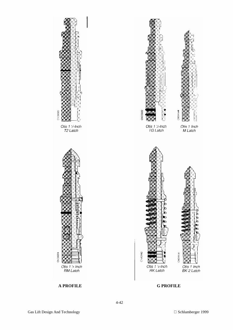
4-42
Gas Lift Design And Technology Schlumberger 1999
A PROFILE G PROFILE
4-43
Gas Lift Design And Technology Schlumberger 1999
Discussion on Latch Profiles
Camco manufactures sidepocket mandrels with both the 'G' and 'A' style profiles as well as the
appropriate latches. Often the question of preference and reliability is raised of one style verses another.
The simple answer to this is there does not appear to be any. Both style of latches are widely used
throughout the world. Aside from specific operational or downhole condition problems both have proved
reliable. Moreover, Camco has discussed this question with the engineers, slickline supervisors and
crews working for numerous North Sea operators. None have highlighted any specific problems with
either type of latch profile.
In recent years the 'G' style latch has progressively become the industry standard, this being especially
true in the North sea. Unless otherwise specified Camco will supply sidepocket mandrels with 'G' style
latch profiles and the appropriate latches.
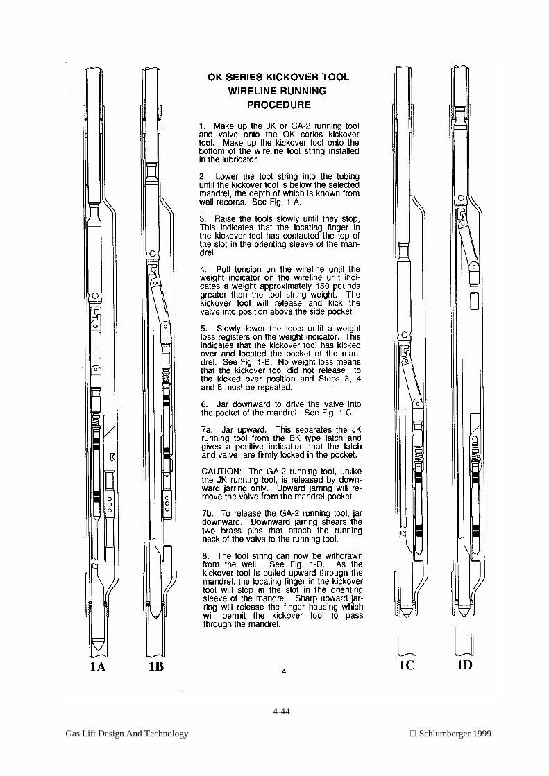
4-44
Gas Lift Design And Technology Schlumberger 1999
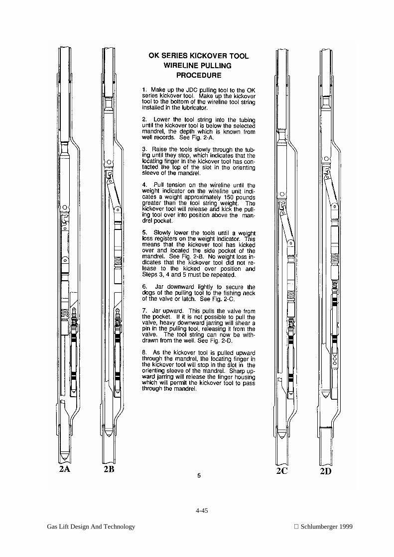
4-45
Gas Lift Design And Technology Schlumberger 1999
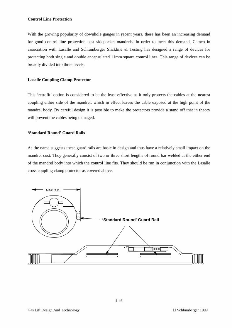
4-46
Gas Lift Design And Technology Schlumberger 1999
Control Line Protection
With the growing popularity of downhole gauges in recent years, there has been an increasing demand
for good control line protection past sidepocket mandrels. In order to meet this demand, Camco in
association with Lasalle and Schlumberger Slickline & Testing has designed a range of devices for
protecting both single and double encapsulated 11mm square control lines. This range of devices can be
broadly divided into three levels:
Lasalle Coupling Clamp Protector
This ‘retrofit’ option is considered to be the least effective as it only protects the cables at the nearest
coupling either side of the mandrel, which in effect leaves the cable exposed at the high point of the
mandrel body. By careful design it is possible to make the protectors provide a stand off that in theory
will prevent the cables being damaged.
‘Standard Round’ Guard Rails
As the name suggests these guard rails are basic in design and thus have a relatively small impact on the
mandrel cost. They generally consist of two or three short lengths of round bar welded at the either end
of the mandrel body into which the control line fits. They should be run in conjunction with the Lasalle
cross coupling clamp protector as covered above.
MAX O.D.
‘Standard Round’ Guard Rail
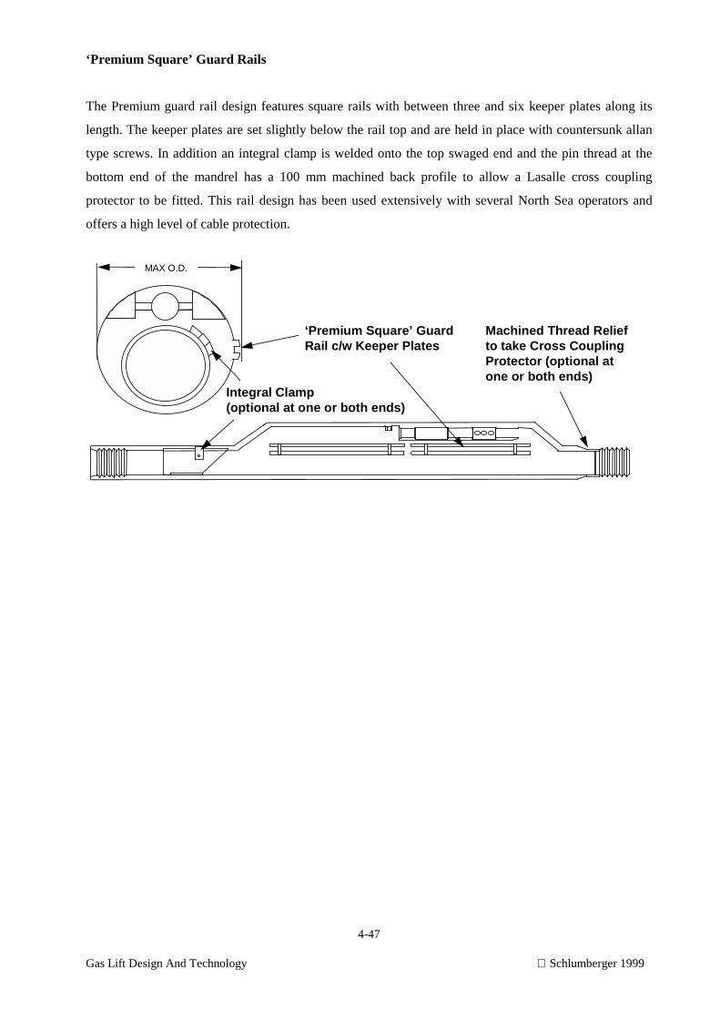
4-47
Gas Lift Design And Technology Schlumberger 1999
‘Premium Square’ Guard Rails
The Premium guard rail design features square rails with between three and six keeper plates along its
length. The keeper plates are set slightly below the rail top and are held in place with countersunk allan
type screws. In addition an integral clamp is welded onto the top swaged end and the pin thread at the
bottom end of the mandrel has a 100 mm machined back profile to allow a Lasalle cross coupling
protector to be fitted. This rail design has been used extensively with several North Sea operators and
offers a high level of cable protection.
MAX O.D.
‘Premium Square’ Guard Rail c/w Keeper Plates
Integral Clamp(optional at one or both ends)
Machined Thread Reliefto take Cross CouplingProtector (optional atone or both ends)
5-1
Gas Lift Design And Technology Schlumberger1999
GAS LIFT DESIGN AND TECHNOLOGY
5. Gas Lift Design
5-2
Gas Lift Design And Technology Schlumberger1999
5A. Manual Design of Continuous Flow Gas Lift Installations
CHAPTER OBJECTIVE: - Given all necessary well data, equations and charts, gas lift
design paper, and necessary equipment, you will design one gas lift installation using
injection pressure operated valves or one utilizing production fluid operated valves. The
design must include:
1. Correct calculation of injection pressure at total depth.
2. The selection of proper flowing gradient curves.
3. The selection of the correct unloading GLR for design.
4. The location of the first valve depth within 25 feet.
5. The use of the proper pressure drop from the injection pressure line.
6. The use of the correct static gradient to space valves to packer or until valve
spacing is less than 300 feet.
7. The use of the correct procedure to select the proper port size.
8. The use of the correct procedure to calculate valve set pressure.
.
INTRODUCTION
The most efficient operation of a gas lift installation depends on proper design. Although the selection of
the valves for the well has been discussed in a previous unit, the spacing of the valves and the
determination of proper pressure setting depends upon accurate design techniques.
Modern design procedures can be accomplished by computer, but gas lift personnel must understand
design fundamentals in order to use these tools effectively. The best method of achieving this
understanding is to personally design a system without computer assistance.
The procedures outlined in this unit are graphical and contain a margin of error. Extreme care must be
taken when reading the design paper and working with gradient curves.
A thorough understanding of design procedures is essential to the gas lift specialist and very helpful to all
others who work with gas lift equipment.
5-3
Gas Lift Design And Technology Schlumberger1999
DESIGN BIAS
The gas lift design process is composed of two stages. They include:
1) The spacing of mandrels and/or gas lift valves, and
2) The calculation of setting pressures for unloading valves.
The objective of the design process is to ensure that the unloading valves are closed when the well is
lifting from the designed operating point. Each of the design techniques presented in this manual has
been developed for the stated objective of achieving single-point injection.
With this in mind, it is often desirable to incorporate various forms of “design bias” into gas lift designs.
This bias is used to ensure that the design is successful in accomplishing the above stated objective. That
is, to ensure that the unloading valves are closed when the well is lifting from the designed operating
point. There are numerous forms of design bias. They include: design bias at the transfer point, casing
pressure bias, temperature bias, FWHP bias, available injection pressure bias and even selection of the
flowing gradient curves.
Transfer Point Bias
One of the most common forms of design bias involves the location of the transfer point (and,
accordingly, the spacing of the mandrels.) This bias is intended to account for uncertainty in the flowing
gradient as it pertains to the unloading process. The transfer point is located using the design bias added
to the tubing pressure at valve depth. There are several different approaches in taking this design bias,
based on different assumptions, as follow:
• A fixed percentage of the differential between the tubing and casing pressure
The rationalle for this approach is that it will bias the transfer point more at the top of the well than
at the bottom of the well. During unloading at the top of the well, we basically u-tube fluid around
from the casing at the top of the well. However, as we work down the well, we begin to get
drawdown on the formation, producing well fluids and formation gas, which aids in the unloading
process. For this reason, biasing the upper mandrels is believed by many to have a greater effect on
the unloading process than biasing the lower mandrels.
• A fixed percentage of the tubing pressure
For the upper unloading valves, there is a certain amount of design bias built-in when the objective
tubing gradient is chosen as the location for the transfer pressures. This is easily illustrated by
generating an equilibrium curve for the well. If we develop an equilibrium curve for the objective
production rate, we will find that the resulting pressures will be considerably less than those found
using the objective tubing gradient. Hense, we have built-in design bias when we use an objective
tubing gradient to design the system. As we move down the hole, the equilibrium curve and
5-4
Gas Lift Design And Technology Schlumberger1999
objective tubing gradient start to converge. Therefore, the greatest uncertainty is not at the upper
unloading valves; but, rather, is at the lower unloading valves. The ultimate result of this method is
that the spacing at the top of the well is relatively unaffected, while the mandrels at the bottom of the
well are forced closer together. A comparison of the various methodologies should also reveal that
this method would actually result in fewer mandrels being placed in the well. This is because the
differential pressure (and spacing) is widest at the top of the well.
• Constant value (50 psi)
This method is a simple and rough approach. It simply involves adding a fixed value to the tubing
pressure at depth to determine the transfer point of each valve.
Other forms of design bias
• FWHP – Engineers often choose to select a flowing wellhead pressure which is higher than what will
be seen in reality. This has the effect of moving the entire objective tubing gradient to the right, and
indirectly does the same thing as the transfer pressure bias discussed above. It may be desirable to
choose a slightly higher wellhead pressure than what is anticipated, so that the well can operate
effectively at higher than normal system pressures.
• Available injection pressure – It is often prudent to design a gas lift installation to operate at a
kickoff pressure which is less than the actual injection pressure available. This will allow the well to
unload even during situations such as compressor shut-downs, low gas sales line pressure, etc.
• Selection of flowing gradient – The selection of the flowing gradient curve can serve as yet another
form of bias. Often, engineers will select a flowing gradient that is “heavier” (or further to the right)
than what is anticipated. In most cases, this requires increasing either the water cut or rate associated
with the curve. However, in applications with complex PVT properties, a more rigorous analysis is
needed to know which gradient to select.
• Temperature bias – Another form of bias involves the selection of design temperatures for the
unloading valves. Since the objective of the gas lift design is to ensure that the upper unloading
valves are closed when the operating point is reached, it is often desirable to take additional
precautions to ensure that this happens. One way to ensure that the this objective is achieved, is to
“temperature lock” the upper unloading valves. This is accomplished by selecting temperatures for
the upper valves that are greater than the static temperature gradient, but less than the flowing
temperature gradient. Since these temperatures are greater than the static temperature gradient, the
valves will open while fluids are being u-tubed from the casing to the tubing. However, once draw-
down is achieved and the well starts to flow, the temperature at depth will be greater than what the
valves were calibrated for, forcing the valves to “lock” closed. When temperature locking valves, it
is important to select temperatures in such a way that the valves are not closed prematurely.
Otherwise, the unloading process will become stymied. For this reason, this is considered an
5-5
Gas Lift Design And Technology Schlumberger1999
advanced design technique and should not be attempted without a thorough understanding of the
processes involved.
Casing pressure (or operating pressure) bias
This is probably the most common form of bias used in a gas lift design and serves as the basis of most
design techniques. We know that in order to ensure that each unloading valve closes when the
successive valve opens, we must take a drop in casing pressure. However, the amount of pressure drop to
take is often in dispute. There are two basic design techniques (and numerous variations) which have
been developed to address this issue. They include the “fixed pressure drop” and “Ppmax – Ppmin”
methods. A summary of these methods and the rationalle behind them follows:
• Constant pressure drop method – This is a very simple method for choosing pressure drops, that is
based in large part on field experience. This method entails taking equal casing pressure drops for all
valves in the design. This pressure drop is generally 10 – 30 psi and is based in large part upon field
experience. An advantage of this method is that it allows the engineer to perform a less conservative
design. This means that an experienced engineer will be able to inject deeper with the same amount
of available injection pressure than they would be able to with the “Ppmax – Ppmin” method. A
draw-back of this method is that it is less technically rigorous than other methods and does not
necessarily incorporate valve mechanics into the design process. For this reason, it is strongly
recommended that individuals using this method double-check their work by back-calculating the
opening and closing pressures under design conditions. The proper application of this technique is
an iterative process involving both valve spacing and calculation of opening and closing pressures.
• “Ppmax-Ppmin“ method – This technique incorporates the relationship between valve mechanics
and spacing in a design. The rationalle and theory behind this design technique follows:
The amount of opening force supplied by production pressure to open the valve is a function of the port
size (PPEF). The effective amount of opening pressure (Peo) supplied by the production pressure is:
Peo = PPEF x Ppd
where Ppd is production pressure acting in valve. This means that pressure acting on the downstream (or
tubing) side of the valve is equivalent to or gives the same effect on the opening the valve as some
fraction of the pressure acting on upstream (or casing) side of the valve. Since the uncontrollable
variable is the production pressure, it is important to approximate the amount it could increase. The
maximum possible flowing production pressure (Ppmax), regardless of flow rate, occurs if the gradient
curve between the flowing wellhead pressure and the injection pressure on the next valve form a straight
line. In reality, this gradient would be curved, making “Ppmax “ greater than what would be seen in
5-6
Gas Lift Design And Technology Schlumberger1999
reality. Therefore this is a certain amount of design bias built into this method. The minimum possible
flowing production pressure (Ppmin) occurs when the well is lifted at the target point of injection. This is
also a conservative approach, because the gradient curve during unloading will never be the same as the
gradient curve during production. During the unloading process, the flowing production pressure will be
between Ppmin and Ppmax, regardless of fluctuations in the flow rate. Therefore any increase in
production pressure will not exceed the value of (Ppmax-Ppmin) and (Ppmax-Ppmin) can represent the
maximum possible increase in production pressure.
To prevent the opening of the valve, the possible increase in production pressure (Ppmax-Ppmin) must be
anticipated by reducing the injection pressure an equivalent value. With this in mind, the casing pressure
for each valve needs to be lowered by the amount of:
PD = PPEF x (Ppmax-Ppmin)
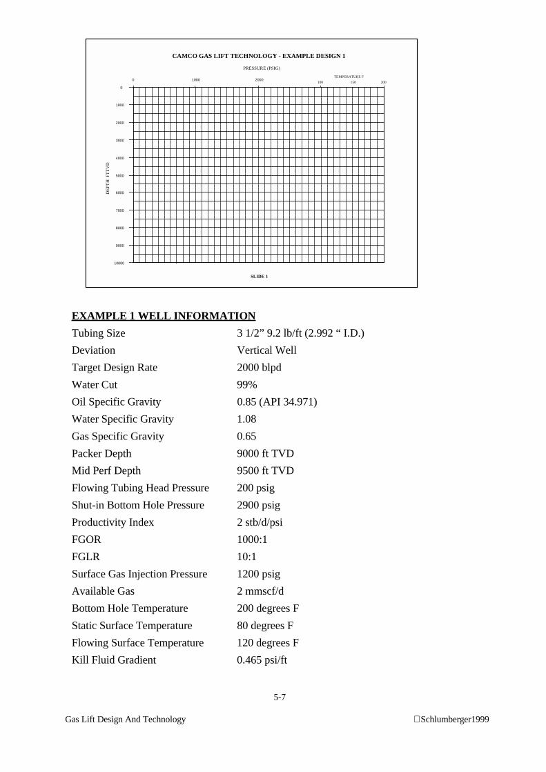
5-7
Gas Lift Design And Technology Schlumberger1999
EXAMPLE 1 WELL INFORMATION
Tubing Size 3 1/2” 9.2 lb/ft (2.992 “ I.D.)
Deviation Vertical Well
Target Design Rate 2000 blpd
Water Cut 99%
Oil Specific Gravity 0.85 (API 34.971)
Water Specific Gravity 1.08
Gas Specific Gravity 0.65
Packer Depth 9000 ft TVD
Mid Perf Depth 9500 ft TVD
Flowing Tubing Head Pressure 200 psig
Shut-in Bottom Hole Pressure 2900 psig
Productivity Index 2 stb/d/psi
FGOR 1000:1
FGLR 10:1
Surface Gas Injection Pressure 1200 psig
Available Gas 2 mmscf/d
Bottom Hole Temperature 200 degrees F
Static Surface Temperature 80 degrees F
Flowing Surface Temperature 120 degrees F
Kill Fluid Gradient 0.465 psi/ft
0 1000 2000
0
1000
2000
3000
4000
5000
6000
7000
8000
9000
10000
PRESSURE (PSIG)
DE
PTH
FT
TV
D
TEMPERATURE F
100 150 200
CAMCO GAS LIFT TECHNOLOGY - EXAMPLE DESIGN 1
SLIDE 1
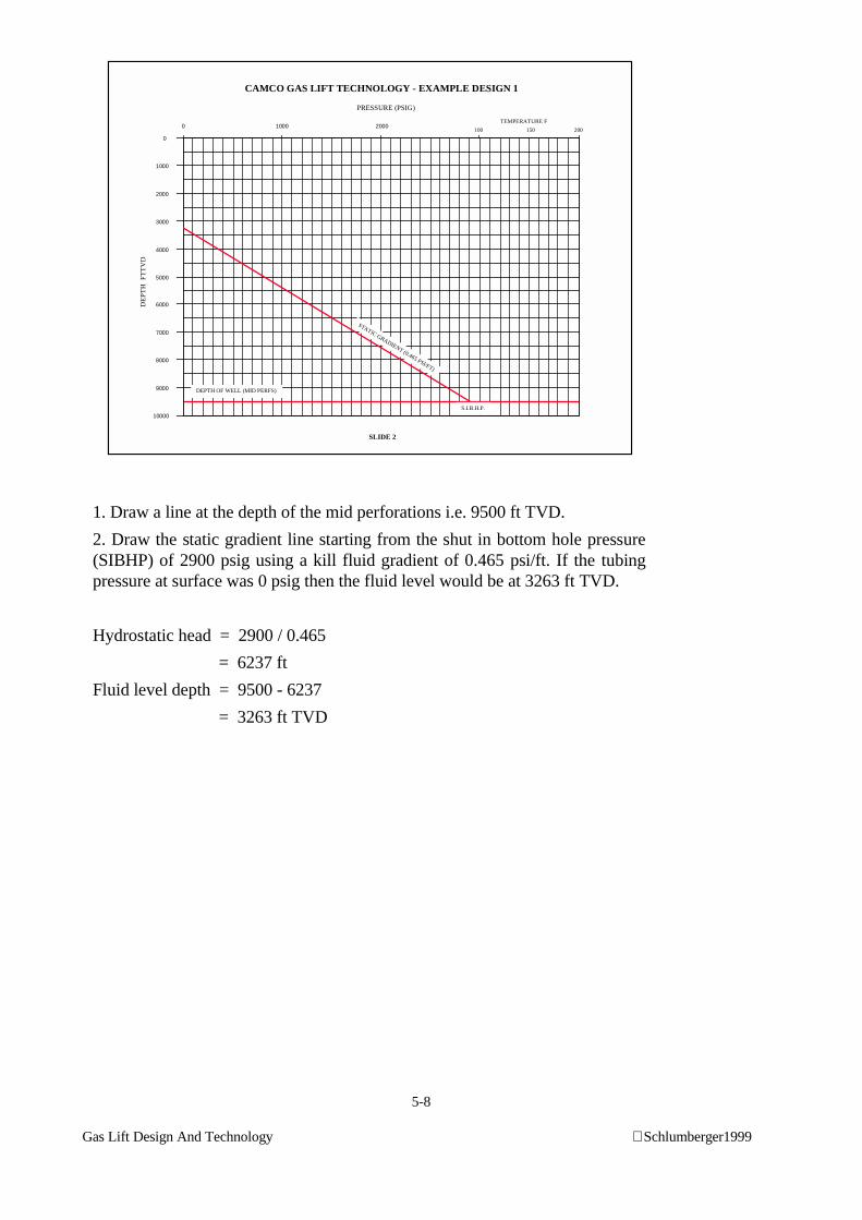
5-8
Gas Lift Design And Technology Schlumberger1999
1. Draw a line at the depth of the mid perforations i.e. 9500 ft TVD.
2. Draw the static gradient line starting from the shut in bottom hole pressure(SIBHP) of 2900 psig using a kill fluid gradient of 0.465 psi/ft. If the tubingpressure at surface was 0 psig then the fluid level would be at 3263 ft TVD.
Hydrostatic head = 2900 / 0.465
= 6237 ft
Fluid level depth = 9500 - 6237
= 3263 ft TVD
0 1000 2000
0
1000
2000
3000
4000
5000
6000
7000
8000
9000
10000
PRESSURE (PSIG)
DE
PT
H F
TT
VD
S.I.B.H.P.
DEPTH OF WELL (MID PERFS)
STATIC GRADIENT (0.465 PSI/FT)
TEMPERATURE F
100 150 200
CAMCO GAS LIFT TECHNOLOGY - EXAMPLE DESIGN 1
SLIDE 2
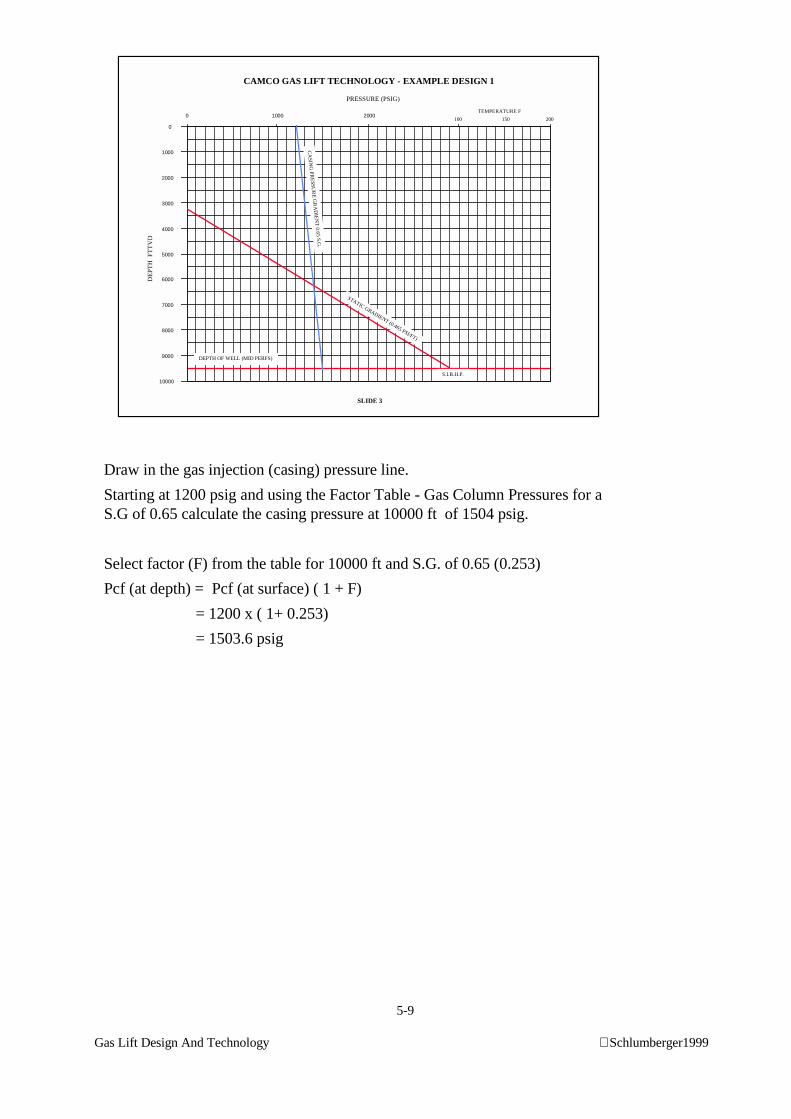
5-9
Gas Lift Design And Technology Schlumberger1999
Draw in the gas injection (casing) pressure line.
Starting at 1200 psig and using the Factor Table - Gas Column Pressures for aS.G of 0.65 calculate the casing pressure at 10000 ft of 1504 psig.
Select factor (F) from the table for 10000 ft and S.G. of 0.65 (0.253)
Pcf (at depth) = Pcf (at surface) ( 1 + F)
= 1200 x ( 1+ 0.253)
= 1503.6 psig
0 1000 2000
0
1000
2000
3000
4000
5000
6000
7000
8000
9000
10000
PRESSURE (PSIG)
DE
PT
H F
TT
VD
S.I.B.H.P.
DEPTH OF WELL (MID PERFS)
STATIC GRADIENT (0.465 PSI/FT)
TEMPERATURE F
100 150 200
CAMCO GAS LIFT TECHNOLOGY - EXAMPLE DESIGN 1
SLIDE 3
CA
SING
PR
ESS
UR
E G
RA
DIE
NT
0.65 S.G.
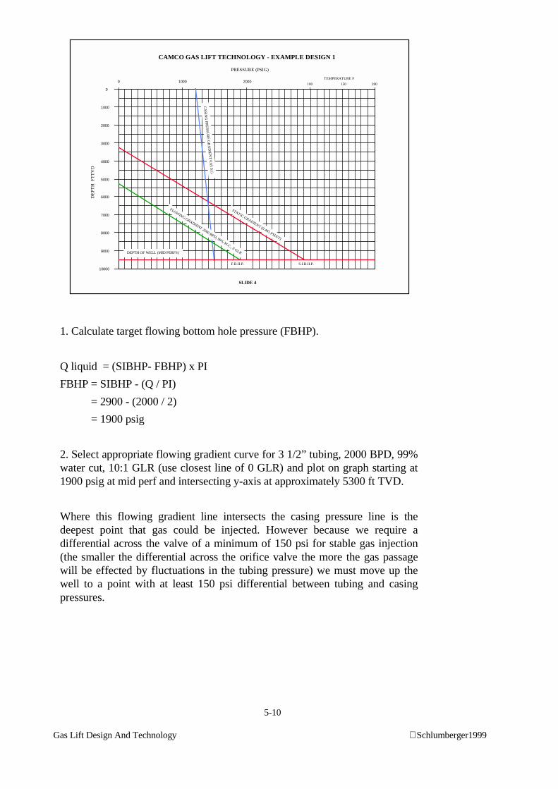
5-10
Gas Lift Design And Technology Schlumberger1999
1. Calculate target flowing bottom hole pressure (FBHP).
Q liquid = (SIBHP- FBHP) x PI
FBHP = SIBHP - (Q / PI)
= 2900 - (2000 / 2)
= 1900 psig
2. Select appropriate flowing gradient curve for 3 1/2” tubing, 2000 BPD, 99%water cut, 10:1 GLR (use closest line of 0 GLR) and plot on graph starting at1900 psig at mid perf and intersecting y-axis at approximately 5300 ft TVD.
Where this flowing gradient line intersects the casing pressure line is thedeepest point that gas could be injected. However because we require adifferential across the valve of a minimum of 150 psi for stable gas injection(the smaller the differential across the orifice valve the more the gas passagewill be effected by fluctuations in the tubing pressure) we must move up thewell to a point with at least 150 psi differential between tubing and casingpressures.
0 1000 2000
0
1000
2000
3000
4000
5000
6000
7000
8000
9000
10000
PRESSURE (PSIG)
DE
PT
H F
TT
VD
S.I.B.H.P.
DEPTH OF WELL (MID PERFS)
STATIC GRADIENT (0.465 PSI/FT)
F.B.H.P.
TEMPERATURE F
100 150 200
CAMCO GAS LIFT TECHNOLOGY - EXAMPLE DESIGN 1
SLIDE 4
FLOWING GRADIENT 2000 BPD, 99% W.C., 0 GLR
CA
SING
PR
ESS
UR
E G
RA
DIE
NT
0.65 S.G.
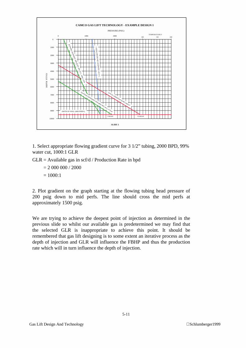
5-11
Gas Lift Design And Technology Schlumberger1999
1. Select appropriate flowing gradient curve for 3 1/2” tubing, 2000 BPD, 99%water cut, 1000:1 GLR
GLR = Available gas in scf/d / Production Rate in bpd
= 2 000 000 / 2000
= 1000:1
2. Plot gradient on the graph starting at the flowing tubing head pressure of200 psig down to mid perfs. The line should cross the mid perfs atapproximately 1500 psig.
We are trying to achieve the deepest point of injection as determined in theprevious slide so whilst our available gas is predetermined we may find thatthe selected GLR is inappropriate to achieve this point. It should beremembered that gas lift designing is to some extent an iterative process as thedepth of injection and GLR will influence the FBHP and thus the productionrate which will in turn influence the depth of injection.
0 1000 2000
0
1000
2000
3000
4000
5000
6000
7000
8000
9000
10000
PRESSURE (PSIG)
DE
PT
H F
TT
VD
S.I.B.H.P.
DEPTH OF WELL (MID PERFS)
STATIC GRADIENT (0.465 PSI/FT)
F.B.H.P.
FLOW
ING
GR
AD
IENT
2000 BL
PD, 99%
W.C
., 1000:1 GL
R
TEMPERATURE F
100 150 200
CAMCO GAS LIFT TECHNOLOGY - EXAMPLE DESIGN 1
SLIDE 5
FLOWING GRADIENT 2000 BPD, 99% W.C., 0 GLR
CA
SING
PR
ESS
UR
E G
RA
DIE
NT
0.65 S.G.
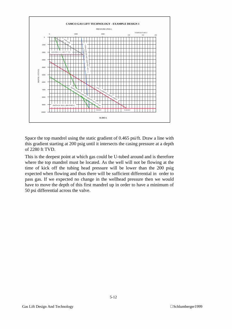
5-12
Gas Lift Design And Technology Schlumberger1999
Space the top mandrel using the static gradient of 0.465 psi/ft. Draw a line withthis gradient starting at 200 psig until it intersects the casing pressure at a depthof 2280 ft TVD.
This is the deepest point at which gas could be U-tubed around and is thereforewhere the top mandrel must be located. As the well will not be flowing at thetime of kick off the tubing head pressure will be lower than the 200 psigexpected when flowing and thus there will be sufficient differential in order topass gas. If we expected no change in the wellhead pressure then we wouldhave to move the depth of this first mandrel up in order to have a minimum of50 psi differential across the valve.
0 1000 2000
0
1000
2000
3000
4000
5000
6000
7000
8000
9000
10000
PRESSURE (PSIG)
DE
PT
H F
TT
VD
S.I.B.H.P.
DEPTH OF WELL (MID PERFS)
STATIC GRADIENT (0.465 PSI/FT)
F.B.H.P.
MANDREL #1, 2280 FT TVD
0.465 psi/ft
TEMPERATURE F
100 150 200
CAMCO GAS LIFT TECHNOLOGY - EXAMPLE DESIGN 1
SLIDE 6
FLOWING GRADIENT 2000 BPD, 99% W.C., 0 GLR
CA
SING
PR
ESS
UR
E G
RA
DIE
NT
0.65 S.G.
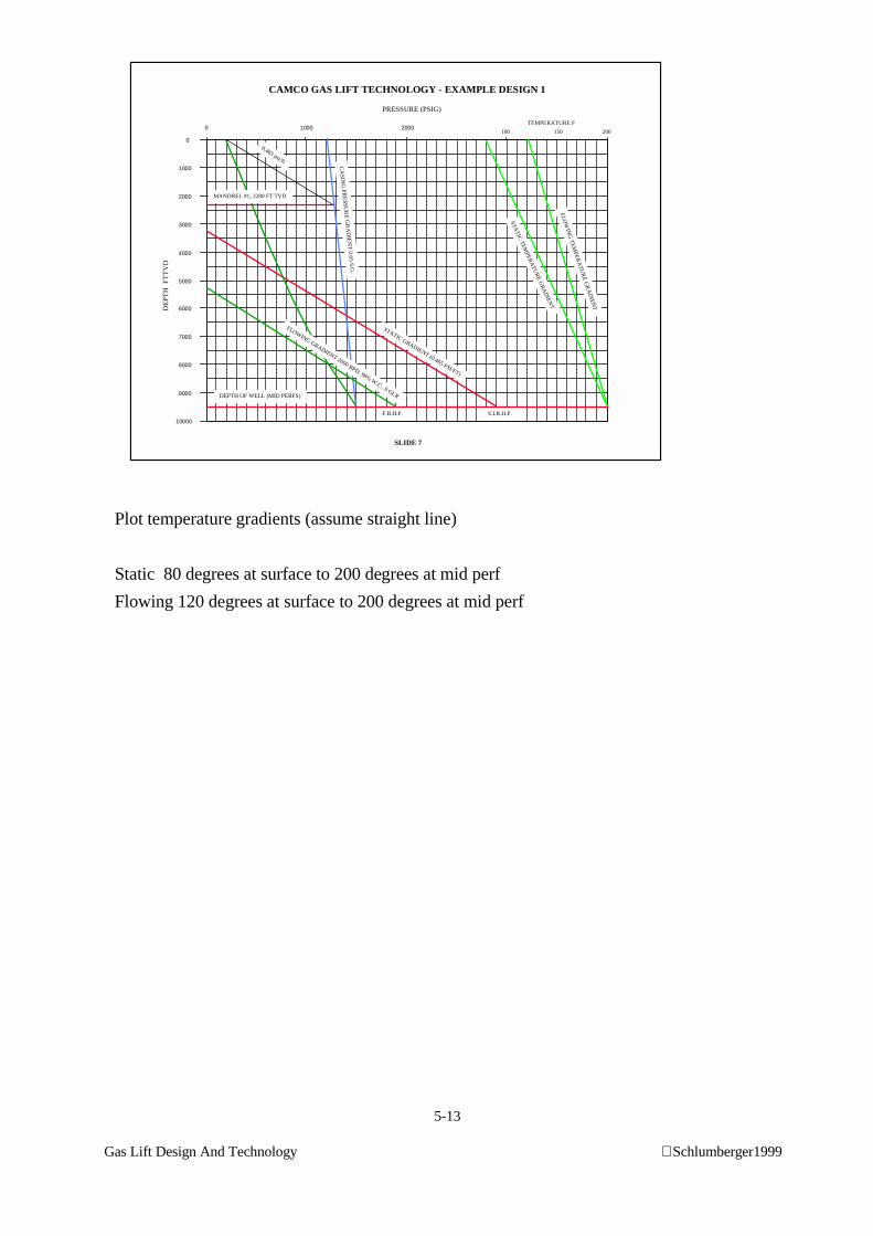
5-13
Gas Lift Design And Technology Schlumberger1999
Plot temperature gradients (assume straight line)
Static 80 degrees at surface to 200 degrees at mid perf
Flowing 120 degrees at surface to 200 degrees at mid perf
0 1000 2000
0
1000
2000
3000
4000
5000
6000
7000
8000
9000
10000
PRESSURE (PSIG)
DE
PT
H F
TT
VD
S.I.B.H.P.
DEPTH OF WELL (MID PERFS)
STATIC GRADIENT (0.465 PSI/FT)
F.B.H.P.
MANDREL #1, 2280 FT TVD
0.465 psi/ft
STAT
IC T
EM
PER
AT
UR
E G
RA
DIE
NT
FLOW
ING
TE
MPE
RA
TUR
E G
RA
DIEN
T
TEMPERATURE F
100 150 200
CAMCO GAS LIFT TECHNOLOGY - EXAMPLE DESIGN 1
SLIDE 7
FLOWING GRADIENT 2000 BPD, 99% W.C., 0 GLR
CA
SING
PR
ESS
UR
E G
RA
DIE
NT
0.65 S.G.
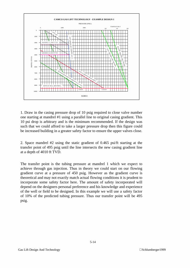
5-14
Gas Lift Design And Technology Schlumberger1999
1. Draw in the casing pressure drop of 10 psig required to close valve numberone starting at mandrel #1 using a parallel line to original casing gradient. This10 psi drop is arbitrary and is the minimum recommended. If the design wassuch that we could afford to take a larger pressure drop then this figure couldbe increased building in a greater safety factor to ensure the upper valves close.
2. Space mandrel #2 using the static gradient of 0.465 psi/ft starting at thetransfer point of 495 psig until the line intersects the new casing gradient lineat a depth of 4010 ft TVD.
The transfer point is the tubing pressure at mandrel 1 which we expect toachieve through gas injection. Thus in theory we could start on our flowinggradient curve at a pressure of 450 psig. However as the gradient curve istheoretical and may not exactly match actual flowing conditions it is prudent toincorporate some safety factor here. The amount of safety incorporated willdepend on the designers personal preference and his knowledge and experienceof the well or field to be designed. In this example we will use a safety factorof 10% of the predicted tubing pressure. Thus our transfer point will be 495psig.
0 1000 2000
0
1000
2000
3000
4000
5000
6000
7000
8000
9000
10000
PRESSURE (PSIG)
DE
PT
H F
TT
VD
S.I.B.H.P.
DEPTH OF WELL (MID PERFS)
STATIC GRADIENT (0.465 PSI/FT)
F.B.H.P.
MANDREL #1, 2280 FT TVD
0.465 psi/ft
MANDREL #2, 4010 FT TVD
TEMPERATURE F
100 150 200
STAT
IC T
EM
PER
AT
UR
E G
RA
DIE
NT
FLOW
ING
TE
MPE
RA
TUR
E G
RA
DIEN
T
CAMCO GAS LIFT TECHNOLOGY - EXAMPLE DESIGN 1
SLIDE 8
FLOWING GRADIENT 2000 BPD, 99% W.C., 0 GLR
CA
SING
PR
ESS
UR
E G
RA
DIE
NT
0.65 S.G.
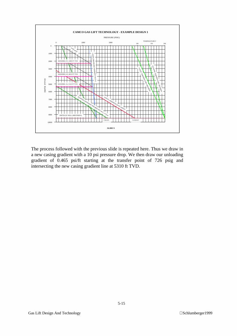
5-15
Gas Lift Design And Technology Schlumberger1999
The process followed with the previous slide is repeated here. Thus we draw ina new casing gradient with a 10 psi pressure drop. We then draw our unloadinggradient of 0.465 psi/ft starting at the transfer point of 726 psig andintersecting the new casing gradient line at 5310 ft TVD.
0 1000 2000
0
1000
2000
3000
4000
5000
6000
7000
8000
9000
10000
PRESSURE (PSIG)
DE
PT
H F
TT
VD
S.I.B.H.P.
DEPTH OF WELL (MID PERFS)
STATIC GRADIENT (0.465 PSI/FT)
F.B.H.P.
MANDREL #1, 2280 FT TVD
0.465 psi/ft
MANDREL #2, 4010 FT TVD
TEMPERATURE F
100 150 200
STAT
IC T
EM
PER
AT
UR
E G
RA
DIE
NT
FLOW
ING
TE
MPE
RA
TUR
E G
RA
DIEN
T
CAMCO GAS LIFT TECHNOLOGY - EXAMPLE DESIGN 1
SLIDE 9
MANDREL #3, 5310 FT TVD
FLOWING GRADIENT 2000 BPD, 99% W.C., 0 GLR
CA
SING
PR
ESS
UR
E G
RA
DIE
NT
0.65 S.G.
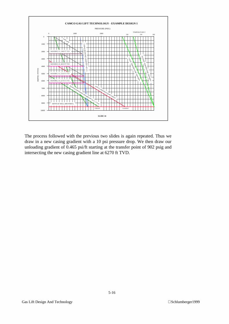
5-16
Gas Lift Design And Technology Schlumberger1999
The process followed with the previous two slides is again repeated. Thus wedraw in a new casing gradient with a 10 psi pressure drop. We then draw ourunloading gradient of 0.465 psi/ft starting at the transfer point of 902 psig andintersecting the new casing gradient line at 6270 ft TVD.
0 1000 2000
0
1000
2000
3000
4000
5000
6000
7000
8000
9000
10000
PRESSURE (PSIG)
DE
PT
H F
TT
VD
S.I.B.H.P.
DEPTH OF WELL (MID PERFS)
STATIC GRADIENT (0.465 PSI/FT)
F.B.H.P.
MANDREL #1, 2280 FT TVD
0.465 psi/ft
MANDREL #2, 4010 FT TVD
TEMPERATURE F
100 150 200
STAT
IC T
EM
PER
AT
UR
E G
RA
DIE
NT
FLOW
ING
TE
MPE
RA
TUR
E G
RA
DIEN
T
CAMCO GAS LIFT TECHNOLOGY - EXAMPLE DESIGN 1
SLIDE 10
MANDREL #3, 5310 FT TVD
MANDREL #4, 6270 FT TVD
FLOWING GRADIENT 2000 BPD, 99% W.C., 0 GLR
CA
SING
PR
ESS
UR
E G
RA
DIE
NT
0.65 S.G.
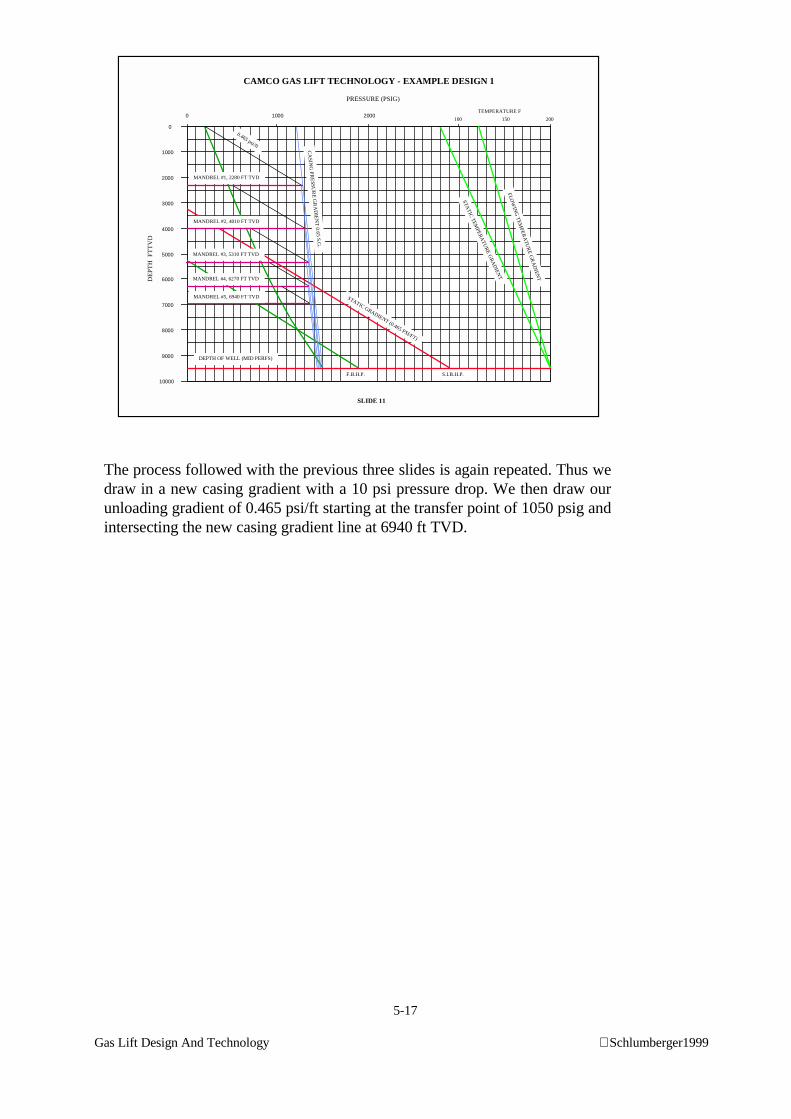
5-17
Gas Lift Design And Technology Schlumberger1999
The process followed with the previous three slides is again repeated. Thus wedraw in a new casing gradient with a 10 psi pressure drop. We then draw ourunloading gradient of 0.465 psi/ft starting at the transfer point of 1050 psig andintersecting the new casing gradient line at 6940 ft TVD.
0 1000 2000
0
1000
2000
3000
4000
5000
6000
7000
8000
9000
10000
PRESSURE (PSIG)
DE
PT
H F
TT
VD
S.I.B.H.P.
DEPTH OF WELL (MID PERFS)
STATIC GRADIENT (0.465 PSI/FT)
F.B.H.P.
MANDREL #1, 2280 FT TVD
0.465 psi/ft
MANDREL #2, 4010 FT TVD
TEMPERATURE F
100 150 200
STAT
IC T
EM
PER
AT
UR
E G
RA
DIE
NT
FLOW
ING
TE
MPE
RA
TUR
E G
RA
DIEN
T
CAMCO GAS LIFT TECHNOLOGY - EXAMPLE DESIGN 1
SLIDE 11
MANDREL #3, 5310 FT TVD
MANDREL #4, 6270 FT TVD
MANDREL #5, 6940 FT TVD
CA
SING
PR
ESS
UR
E G
RA
DIE
NT
0.65 S.G.
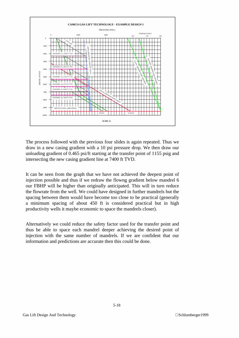
5-18
Gas Lift Design And Technology Schlumberger1999
The process followed with the previous four slides is again repeated. Thus wedraw in a new casing gradient with a 10 psi pressure drop. We then draw ourunloading gradient of 0.465 psi/ft starting at the transfer point of 1155 psig andintersecting the new casing gradient line at 7400 ft TVD.
It can be seen from the graph that we have not achieved the deepest point ofinjection possible and thus if we redraw the flowng gradient below mandrel 6our FBHP will be higher than originally anticipated. This will in turn reducethe flowrate from the well. We could have designed in further mandrels but thespacing between them would have become too close to be practical (generallya minimum spacing of about 450 ft is considered practical but in highproductivity wells it maybe economic to space the mandrels closer).
Alternatively we could reduce the safety factor used for the transfer point andthus be able to space each mandrel deeper achieving the desired point ofinjection with the same number of mandrels. If we are confident that ourinformation and predictions are accurate then this could be done.
0 1000 2000
0
1000
2000
3000
4000
5000
6000
7000
8000
9000
10000
PRESSURE (PSIG)
DE
PT
H F
TT
VD
S.I.B.H.P.
DEPTH OF WELL (MID PERFS)
STATIC GRADIENT (0.465 PSI/FT)
F.B.H.P.
MANDREL #1, 2280 FT TVD
0.465 psi/ft
MANDREL #2, 4010 FT TVD
TEMPERATURE F
100 150 200
STAT
IC T
EM
PER
AT
UR
E G
RA
DIE
NT
FLOW
ING
TE
MPE
RA
TUR
E G
RA
DIEN
T
CAMCO GAS LIFT TECHNOLOGY - EXAMPLE DESIGN 1
SLIDE 12
MANDREL #3, 5310 FT TVD
MANDREL #4, 6270 FT TVD
MANDREL #5, 6940 FT TVD
MANDREL #6, 7400 FT TVD
CA
SING
PR
ESS
UR
E G
RA
DIE
NT
0.65 S.G.
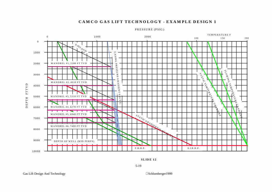
5-19
Gas Lift Design And Technology Schlumberger1999
0 1 00 0 2 00 0
0
1 00 0
2 00 0
3 00 0
4 00 0
5 00 0
6 00 0
7 00 0
8 00 0
9 00 0
1 00 0 0
P R E S S U R E (P S IG )D
EP
TH
F
TT
VD
S .I.B .H .P .
D E P T H O F W E L L (M ID P E R F S )
S T A T IC G R A D IE N T (0 .4 65 P S I/F T )
F .B .H .P .
M A N D R E L # 1 , 2 2 8 0 F T T V D
0 .465 p s i/f t
M A N D R E L # 2 , 4 0 1 0 F T T V D
T E M P E R A T U R E F
1 0 0 1 5 0 2 0 0
ST
AT
IC T
EM
PE
RA
TU
RE
GR
AD
IEN
T
FL
OW
ING
TE
MP
ER
AT
UR
E G
RA
DIE
NT
C A M C O G A S L IF T T E C H N O L O G Y - E X A M P L E D E S IG N 1
S L ID E 1 2
M A N D R E L # 3 , 5 3 1 0 F T T V D
M A N D R E L # 4 , 6 2 7 0 F T T V D
M A N D R E L # 5 , 6 9 4 0 F T T V D
M A N D R E L # 6 , 7 4 0 0 F T T V D
CA
SIN
G P
RE
SS
UR
E G
RA
DIE
NT
0.6
5 S
.G.
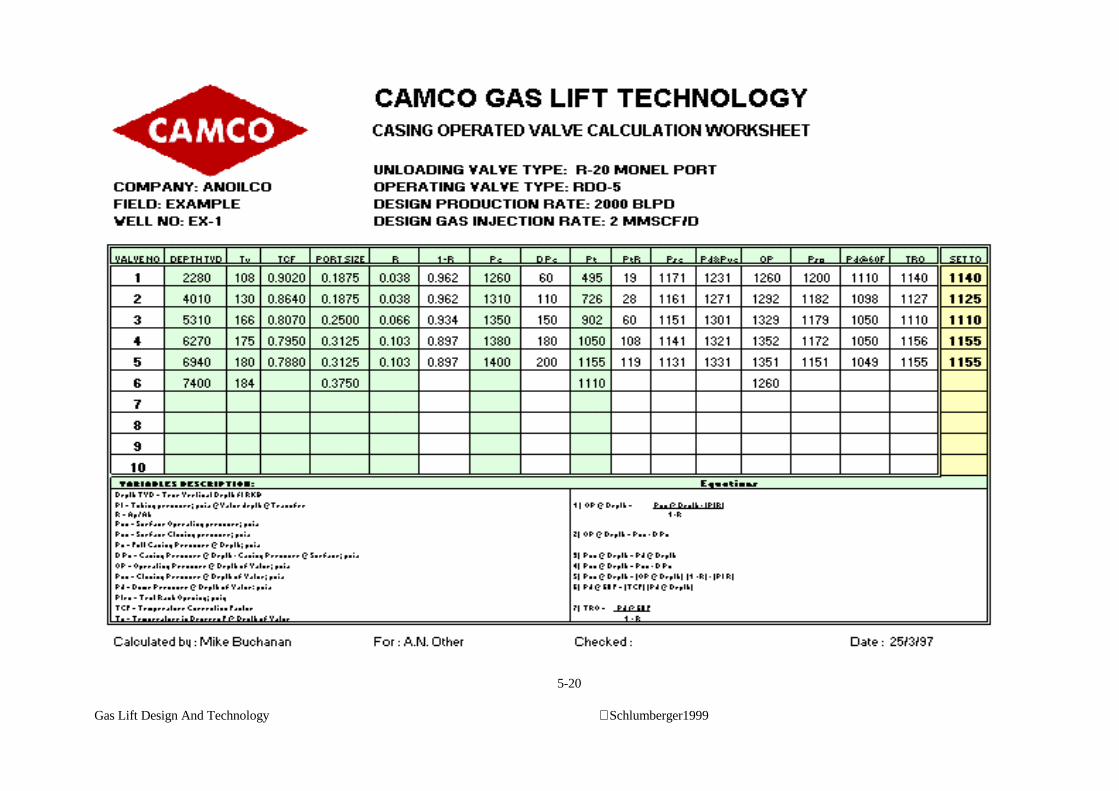
5-20
Gas Lift Design And Technology Schlumberger1999
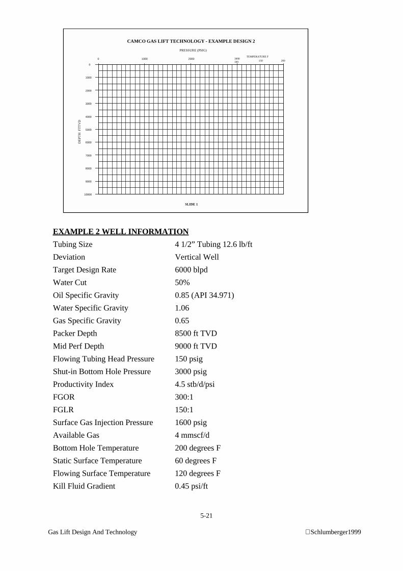
5-21
Gas Lift Design And Technology Schlumberger1999
0 1000 2000
0
1000
2000
3000
4000
5000
6000
7000
8000
9000
10000
PRESSURE (PSIG)
DE
PTH
FT
TV
D
TEMPERATURE F
150 200
CAMCO GAS LIFT TECHNOLOGY - EXAMPLE DESIGN 2
SLIDE 1
3000100
EXAMPLE 2 WELL INFORMATION
Tubing Size 4 1/2” Tubing 12.6 lb/ft
Deviation Vertical Well
Target Design Rate 6000 blpd
Water Cut 50%
Oil Specific Gravity 0.85 (API 34.971)
Water Specific Gravity 1.06
Gas Specific Gravity 0.65
Packer Depth 8500 ft TVD
Mid Perf Depth 9000 ft TVD
Flowing Tubing Head Pressure 150 psig
Shut-in Bottom Hole Pressure 3000 psig
Productivity Index 4.5 stb/d/psi
FGOR 300:1
FGLR 150:1
Surface Gas Injection Pressure 1600 psig
Available Gas 4 mmscf/d
Bottom Hole Temperature 200 degrees F
Static Surface Temperature 60 degrees F
Flowing Surface Temperature 120 degrees F
Kill Fluid Gradient 0.45 psi/ft
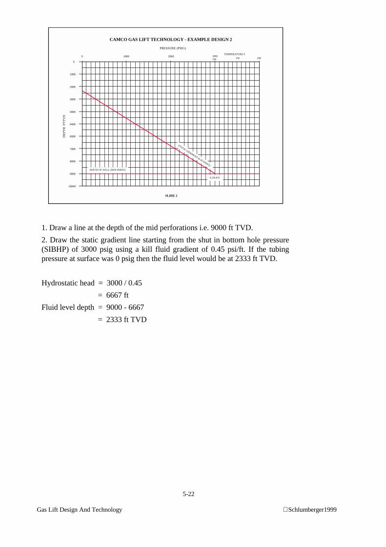
5-22
Gas Lift Design And Technology Schlumberger1999
0 1000 2000
0
1000
2000
3000
4000
5000
6000
7000
8000
9000
10000
PRESSURE (PSIG)
DE
PT
H F
TT
VD
TEMPERATURE F3000100 150 200
CAMCO GAS LIFT TECHNOLOGY - EXAMPLE DESIGN 2
SLIDE 2
S.I.B.H.P.
DEPTH OF WELL (MID PERFS)
STATIC GRADIENT (0.45 PSI/FT)
1. Draw a line at the depth of the mid perforations i.e. 9000 ft TVD.
2. Draw the static gradient line starting from the shut in bottom hole pressure(SIBHP) of 3000 psig using a kill fluid gradient of 0.45 psi/ft. If the tubingpressure at surface was 0 psig then the fluid level would be at 2333 ft TVD.
Hydrostatic head = 3000 / 0.45
= 6667 ft
Fluid level depth = 9000 - 6667
= 2333 ft TVD
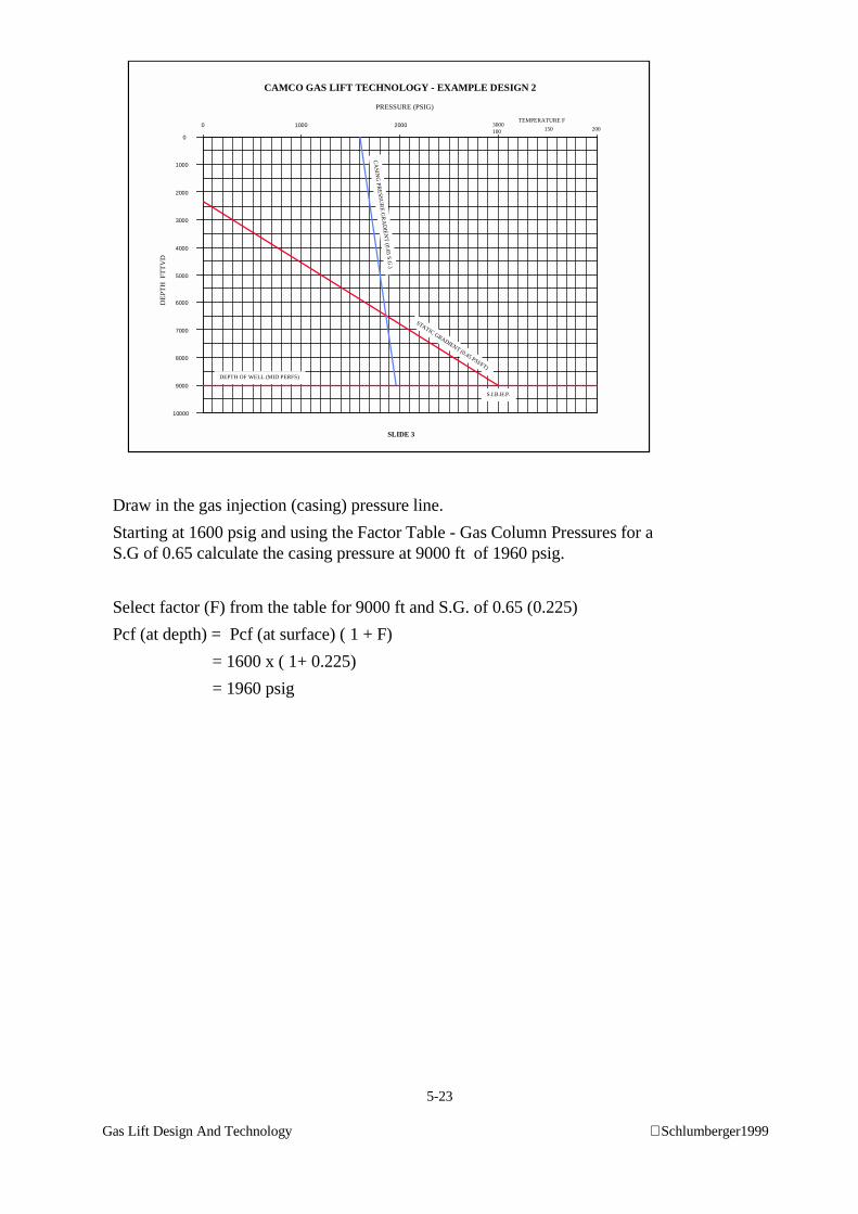
5-23
Gas Lift Design And Technology Schlumberger1999
0 1000 2000
0
1000
2000
3000
4000
5000
6000
7000
8000
9000
10000
PRESSURE (PSIG)
DE
PT
H F
TT
VD
TEMPERATURE F3000100 150 200
CAMCO GAS LIFT TECHNOLOGY - EXAMPLE DESIGN 2
SLIDE 3
S.I.B.H.P.
STATIC GRADIENT (0.45 PSI/FT)
DEPTH OF WELL (MID PERFS)
CA
SING
PR
ESS
UR
E G
RA
DIE
NT
(0.65 S.G
.)
Draw in the gas injection (casing) pressure line.
Starting at 1600 psig and using the Factor Table - Gas Column Pressures for aS.G of 0.65 calculate the casing pressure at 9000 ft of 1960 psig.
Select factor (F) from the table for 9000 ft and S.G. of 0.65 (0.225)
Pcf (at depth) = Pcf (at surface) ( 1 + F)
= 1600 x ( 1+ 0.225)
= 1960 psig
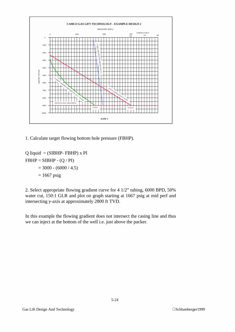
5-24
Gas Lift Design And Technology Schlumberger1999
0 1000 2000
0
1000
2000
3000
4000
5000
6000
7000
8000
9000
10000
PRESSURE (PSIG)
DE
PT
H F
TT
VD
TEMPERATURE F3000100 150 200
CAMCO GAS LIFT TECHNOLOGY - EXAMPLE DESIGN 2
SLIDE 4
S.I.B.H.P.
STATIC GRADIENT (0.45 PSI/FT)
DEPTH OF WELL (MID PERFS)
CA
SING
PR
ESS
UR
E G
RA
DIE
NT
(0.65 S.G
.)
FLOWING GRADIENT 6000 BPD, 50% W
.C., 150 GLR
F.B.H.P.
1. Calculate target flowing bottom hole pressure (FBHP).
Q liquid = (SIBHP- FBHP) x PI
FBHP = SIBHP - (Q / PI)
= 3000 - (6000 / 4.5)
= 1667 psig
2. Select appropriate flowing gradient curve for 4 1/2” tubing, 6000 BPD, 50%water cut, 150:1 GLR and plot on graph starting at 1667 psig at mid perf andintersecting y-axis at approximately 2800 ft TVD.
In this example the flowing gradient does not intersect the casing line and thuswe can inject at the bottom of the well i.e. just above the packer.
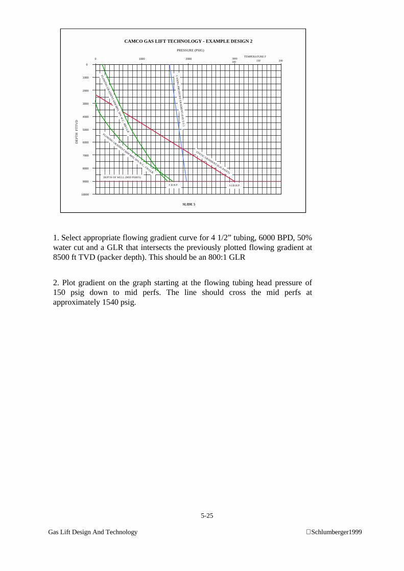
5-25
Gas Lift Design And Technology Schlumberger1999
0 1000 2000
0
1000
2000
3000
4000
5000
6000
7000
8000
9000
10000
PRESSURE (PSIG)
DE
PT
H F
TT
VD
TEMPERATURE F3000100 150 200
CAMCO GAS LIFT TECHNOLOGY - EXAMPLE DESIGN 2
SLIDE 5
S.I.B.H.P.
STATIC GRADIENT (0.45 PSI/FT)
DEPTH OF WELL (MID PERFS)
CA
SING
PR
ESS
UR
E G
RA
DIE
NT
(0.65 S.G
.)
F.B.H.P.
FLOWING GRADIENT 6000 BPD, 50% W
.C., 150 GLR
FLOW
ING
GR
AD
IENT
6000 BPD
, 50% W
.C., 800 G
LR
1. Select appropriate flowing gradient curve for 4 1/2” tubing, 6000 BPD, 50%water cut and a GLR that intersects the previously plotted flowing gradient at8500 ft TVD (packer depth). This should be an 800:1 GLR
2. Plot gradient on the graph starting at the flowing tubing head pressure of150 psig down to mid perfs. The line should cross the mid perfs atapproximately 1540 psig.
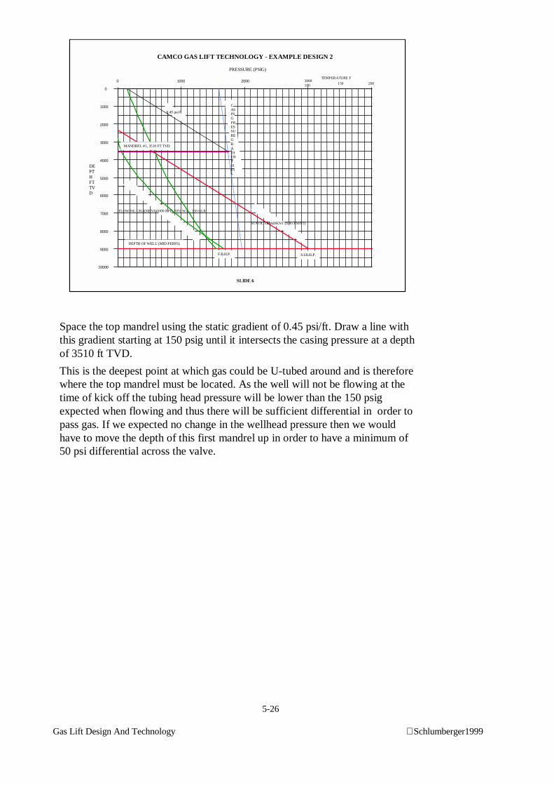
5-26
Gas Lift Design And Technology Schlumberger1999
0 1000 2000
0
1000
2000
3000
4000
5000
6000
7000
8000
9000
10000
PRESSURE (PSIG)
DEPTHFTTVD
TEMPERATURE F3000100 150 200
CAMCO GAS LIFT TECHNOLOGY - EXAMPLE DESIGN 2
SLIDE 6
S.I.B.H.P.
STATIC GRADIENT (0.45 PSI/FT)
DEPTH OF WELL (MID PERFS)
CASINGPRESSUREGRADIENT(0.65S.
F.B.H.P.
FLOWING GRADIENT 6000 BPD, 50% W.C., 150 GLR
0.45 psi/ft
MANDREL #1, 3510 FT TVD
Space the top mandrel using the static gradient of 0.45 psi/ft. Draw a line withthis gradient starting at 150 psig until it intersects the casing pressure at a depthof 3510 ft TVD.
This is the deepest point at which gas could be U-tubed around and is thereforewhere the top mandrel must be located. As the well will not be flowing at thetime of kick off the tubing head pressure will be lower than the 150 psigexpected when flowing and thus there will be sufficient differential in order topass gas. If we expected no change in the wellhead pressure then we wouldhave to move the depth of this first mandrel up in order to have a minimum of50 psi differential across the valve.
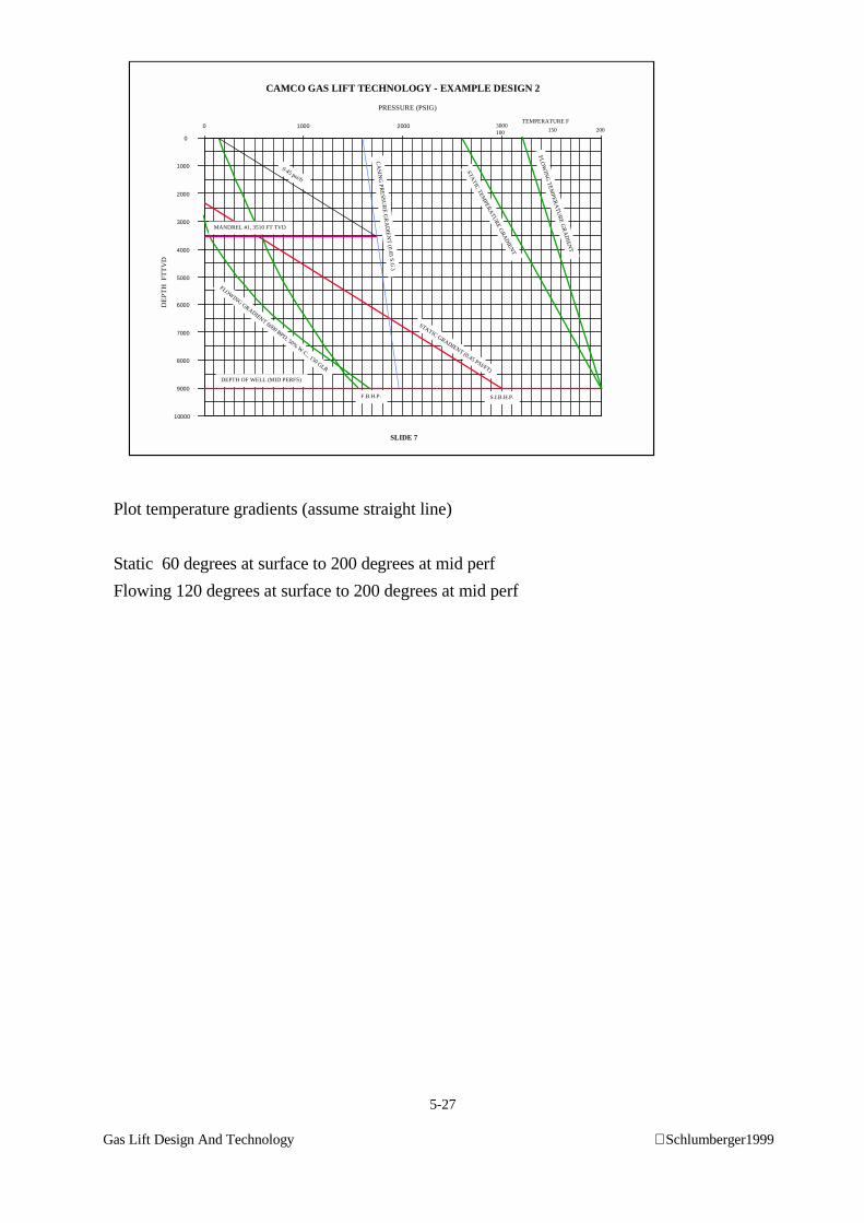
5-27
Gas Lift Design And Technology Schlumberger1999
0 1000 2000
0
1000
2000
3000
4000
5000
6000
7000
8000
9000
10000
PRESSURE (PSIG)
DE
PT
H F
TT
VD
TEMPERATURE F3000100 150 200
CAMCO GAS LIFT TECHNOLOGY - EXAMPLE DESIGN 2
SLIDE 7
S.I.B.H.P.
STATIC GRADIENT (0.45 PSI/FT)
DEPTH OF WELL (MID PERFS)
CA
SING
PR
ESS
UR
E G
RA
DIE
NT
(0.65 S.G
.)
F.B.H.P.
FLOWING GRADIENT 6000 BPD, 50% W
.C., 150 GLR
0.45 psi/ft
MANDREL #1, 3510 FT TVD
STAT
IC TEM
PER
AT
UR
E G
RA
DIE
NT
FL
OW
ING
TE
MP
ER
AT
UR
E G
RA
DIE
NT
Plot temperature gradients (assume straight line)
Static 60 degrees at surface to 200 degrees at mid perf
Flowing 120 degrees at surface to 200 degrees at mid perf
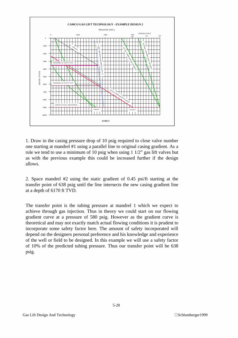
5-28
Gas Lift Design And Technology Schlumberger1999
0 1000 2000
0
1000
2000
3000
4000
5000
6000
7000
8000
9000
10000
PRESSURE (PSIG)
DE
PT
H F
TT
VD
TEMPERATURE F3000100 150 200
CAMCO GAS LIFT TECHNOLOGY - EXAMPLE DESIGN 2
SLIDE 8
S.I.B.H.P.
STATIC GRADIENT (0.45 PSI/FT)
DEPTH OF WELL (MID PERFS)
CA
SING
PR
ESS
UR
E G
RA
DIE
NT
(0.65 S.G
.)
F.B.H.P.
0.45 psi/ft
MANDREL #1, 3510 FT TVD
MANDREL #2, 6170 FT TVD
STAT
IC TEM
PER
AT
UR
E G
RA
DIE
NT
FL
OW
ING
TE
MP
ER
AT
UR
E G
RA
DIE
NT
1. Draw in the casing pressure drop of 10 psig required to close valve numberone starting at mandrel #1 using a parallel line to original casing gradient. As arule we tend to use a minimum of 10 psig when using 1 1/2” gas lift valves butas with the previous example this could be increased further if the designallows.
2. Space mandrel #2 using the static gradient of 0.45 psi/ft starting at thetransfer point of 638 psig until the line intersects the new casing gradient lineat a depth of 6170 ft TVD.
The transfer point is the tubing pressure at mandrel 1 which we expect toachieve through gas injection. Thus in theory we could start on our flowinggradient curve at a pressure of 580 psig. However as the gradient curve istheoretical and may not exactly match actual flowing conditions it is prudent toincorporate some safety factor here. The amount of safety incorporated willdepend on the designers personal preference and his knowledge and experienceof the well or field to be designed. In this example we will use a safety factorof 10% of the predicted tubing pressure. Thus our transfer point will be 638psig.
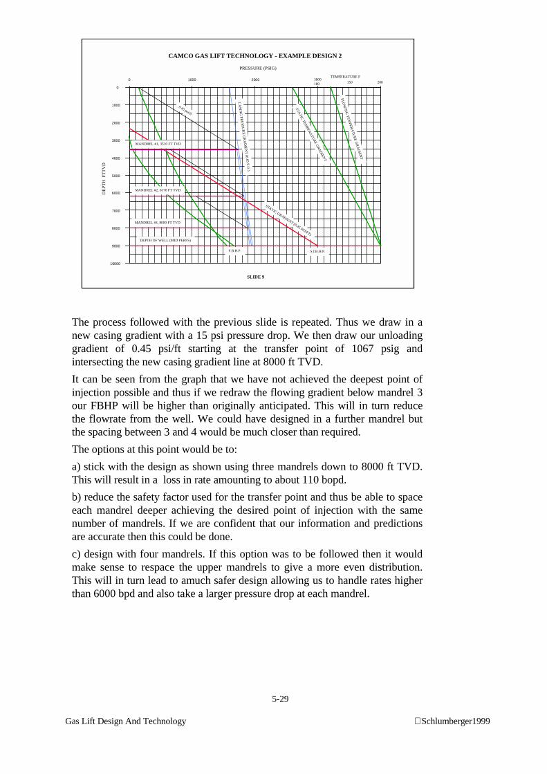
5-29
Gas Lift Design And Technology Schlumberger1999
0 1000 2000
0
1000
2000
3000
4000
5000
6000
7000
8000
9000
10000
PRESSURE (PSIG)
DE
PT
H F
TT
VD
TEMPERATURE F3000100 150 200
CAMCO GAS LIFT TECHNOLOGY - EXAMPLE DESIGN 2
SLIDE 9
S.I.B.H.P.
STATIC GRADIENT (0.45 PSI/FT)
DEPTH OF WELL (MID PERFS)
CA
SING
PR
ESS
UR
E G
RA
DIE
NT
(0.65 S.G
.)
F.B.H.P.
0.45 psi/ft
MANDREL #1, 3510 FT TVD
MANDREL #2, 6170 FT TVD
STAT
IC TEM
PER
AT
UR
E G
RA
DIE
NT
FL
OW
ING
TE
MP
ER
AT
UR
E G
RA
DIE
NT
MANDREL #3, 8000 FT TVD
The process followed with the previous slide is repeated. Thus we draw in anew casing gradient with a 15 psi pressure drop. We then draw our unloadinggradient of 0.45 psi/ft starting at the transfer point of 1067 psig andintersecting the new casing gradient line at 8000 ft TVD.
It can be seen from the graph that we have not achieved the deepest point ofinjection possible and thus if we redraw the flowing gradient below mandrel 3our FBHP will be higher than originally anticipated. This will in turn reducethe flowrate from the well. We could have designed in a further mandrel butthe spacing between 3 and 4 would be much closer than required.
The options at this point would be to:
a) stick with the design as shown using three mandrels down to 8000 ft TVD.This will result in a loss in rate amounting to about 110 bopd.
b) reduce the safety factor used for the transfer point and thus be able to spaceeach mandrel deeper achieving the desired point of injection with the samenumber of mandrels. If we are confident that our information and predictionsare accurate then this could be done.
c) design with four mandrels. If this option was to be followed then it wouldmake sense to respace the upper mandrels to give a more even distribution.This will in turn lead to amuch safer design allowing us to handle rates higherthan 6000 bpd and also take a larger pressure drop at each mandrel.
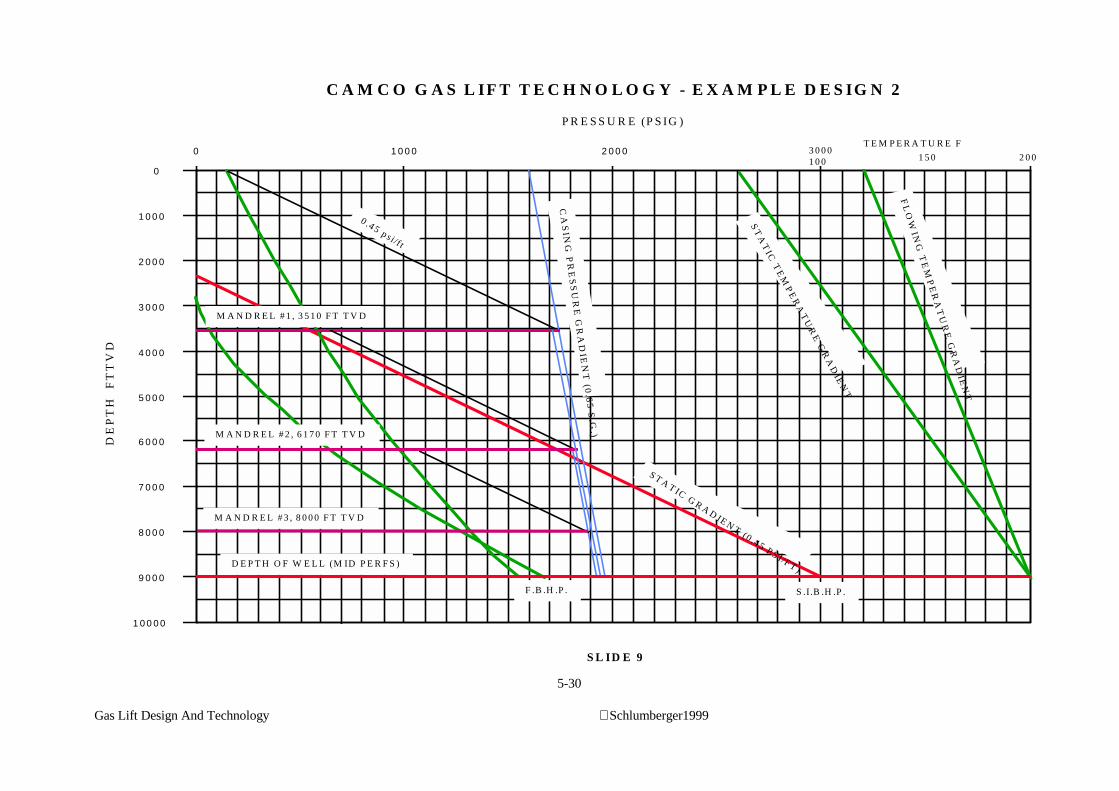
5-30
Gas Lift Design And Technology Schlumberger1999
0 1 0 0 0 2 0 0 0
0
1 0 0 0
2 0 0 0
3 0 0 0
4 0 0 0
5 0 0 0
6 0 0 0
7 0 0 0
8 0 0 0
9 0 0 0
1 0 0 0 0
P R E S S U R E (P S IG )D
EP
TH
F
TT
VD
T E M P E R A T U R E F3 0 0 01 0 0 1 5 0 2 0 0
C A M C O G A S L IF T T E C H N O L O G Y - E X A M P L E D E S IG N 2
S L ID E 9
S .I.B .H .P .
S T A T IC G R A D IE N T (0 .4 5 P S I/F T )D E P T H O F W E L L (M ID P E R F S )C
AS
ING
PR
ES
SU
RE
GR
AD
IEN
T (0
.65
S.G
.)
F .B .H .P .
0 .4 5 p s i /f t
M A N D R E L # 1 , 3 5 1 0 F T T V D
M A N D R E L # 2 , 6 1 7 0 F T T V D
ST
AT
IC T
EM
PE
RA
TU
RE
GR
AD
IEN
T
FL
OW
ING
TE
MP
ER
AT
UR
E G
RA
DIE
NT
M A N D R E L # 3 , 8 0 0 0 F T T V D
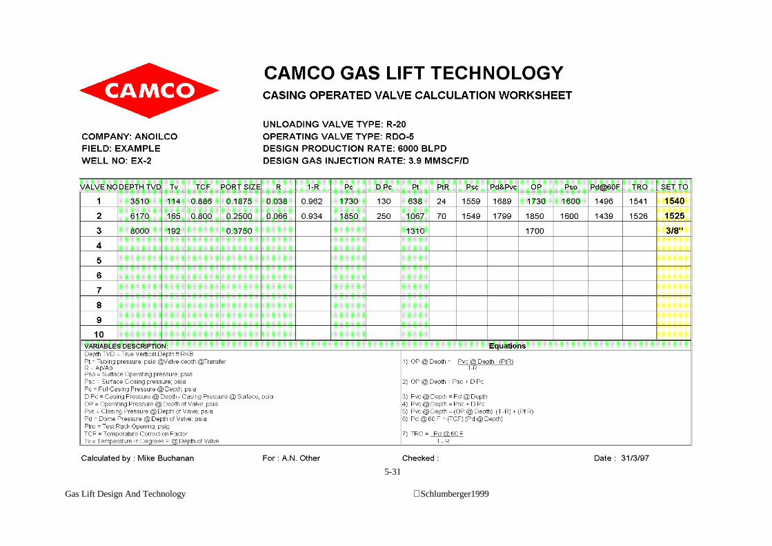
5-31
Gas Lift Design And Technology Schlumberger1999
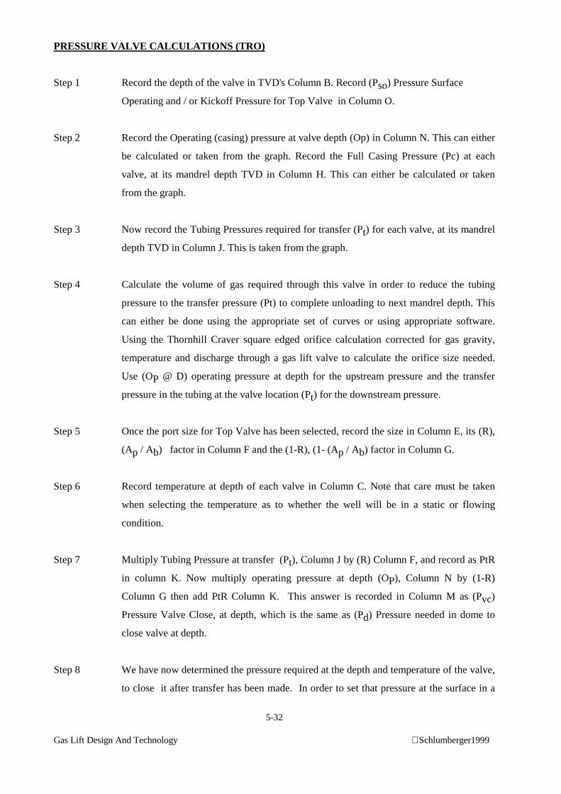
5-32
Gas Lift Design And Technology Schlumberger1999
PRESSURE VALVE CALCULATIONS (TRO)
Step 1 Record the depth of the valve in TVD's Column B. Record (Pso) Pressure Surface
Operating and / or Kickoff Pressure for Top Valve in Column O.
Step 2 Record the Operating (casing) pressure at valve depth (Op) in Column N. This can either
be calculated or taken from the graph. Record the Full Casing Pressure (Pc) at each
valve, at its mandrel depth TVD in Column H. This can either be calculated or taken
from the graph.
Step 3 Now record the Tubing Pressures required for transfer (Pt) for each valve, at its mandrel
depth TVD in Column J. This is taken from the graph.
Step 4 Calculate the volume of gas required through this valve in order to reduce the tubing
pressure to the transfer pressure (Pt) to complete unloading to next mandrel depth. This
can either be done using the appropriate set of curves or using appropriate software.
Using the Thornhill Craver square edged orifice calculation corrected for gas gravity,
temperature and discharge through a gas lift valve to calculate the orifice size needed.
Use (OP @ D) operating pressure at depth for the upstream pressure and the transfer
pressure in the tubing at the valve location (Pt) for the downstream pressure.
Step 5 Once the port size for Top Valve has been selected, record the size in Column E, its (R),
(Ap / Ab) factor in Column F and the (1-R), (1- (Ap / Ab) factor in Column G.
Step 6 Record temperature at depth of each valve in Column C. Note that care must be taken
when selecting the temperature as to whether the well will be in a static or flowing
condition.
Step 7 Multiply Tubing Pressure at transfer (Pt), Column J by (R) Column F, and record as PtR
in column K. Now multiply operating pressure at depth (OP), Column N by (1-R)
Column G then add PtR Column K. This answer is recorded in Column M as (Pvc)
Pressure Valve Close, at depth, which is the same as (Pd) Pressure needed in dome to
close valve at depth.
Step 8 We have now determined the pressure required at the depth and temperature of the valve,
to close it after transfer has been made. In order to set that pressure at the surface in a
5-33
Gas Lift Design And Technology Schlumberger1999
shop environment, we must now convert that pressure to 60oF from downhole flowing
temperature. In order to do this we must first determine the temperature correction factor
from the Correction Factor Chart and record in Column D. We then multiply the
appropriate temperature correction factor, Column D, by the (Pvc or Pd) Column M and
record the answer in Pd at 600F Column P.
Step 9 The pressure in Column P, Pd at 600 , only needs to be divided by the (1-R) Column G
to achieve final Test Rack Opening Pressure in psia. As the valve will be set up to psig
subtract 14.5 from this answer. This step converts the Pd at 600F in psia to the pressure
directed on the effective area that Pd at 600F is acting on.
Step 10 Subtract operating casing pressure at surface (Pso) Column O from full casing pressure
at depth (Pc) Column H to obtain the (Dpc) Column I.
Step 11 Subtract (Dpc) Column I from pressure valve closing or dome pressure (Pd & Pvc)
Column M to obtain surface closing pressure Column L.
Step 12 NOTE: PROCEED TO STEP 13 IF NO KICKOFF PRESSURE USED
If a kickoff pressure was used for valve #1 then valve #2 follows exactly the same steps 1
through 11, the only difference being the lower casing pressure.
Step 13 For the next valve we can now choose our surface closing pressure instead of it being
determined by the surface conditions as in valves #1 (and #2 if kick-off pressure used).
In order to ensure the valve above closes after this valve is uncovered, we must make
sure there is a 10-50 psi drop in surface closing pressure (Psc) Column L. Use 10 psi as
a minimum but remember the larger the pressure drop the safer the design. However this
pressure drop should be such that injection depth is not seriously compromised. So now
in order to calculate the rest of the valves, we will simply drop each surface closing
pressure 10 psi per valve station. Record this pressure in Column L.
Step 14 Subtract Surface Operating Pressure, Pso, Column O, from the Full Casing Pressure at
this valve Pc, Column H, and record as Dpc in Column I. Add this weight of gas to the
surface closing pressure (Psc) in Column L to give Pd&Pvc, Column M.
5-34
Gas Lift Design And Technology Schlumberger1999
Step 15 Calculate the volume of gas required as per step 4 and size port accordingly. Record R,
Column F, and (1-R), Column G.
Step 16 Multiply the appropriate temperature correction factor Column D by the Pvc Column M.
Record answer in Column P, Pd at 60oF.
Step 17 Divide Pd at 60oF, Column P by the (1-R) Column G, subtract 14.5 and record your
answer in TRO, Column Q.
Step 18 Now multiply Pt Column J by R Column F and record in Column K. Subtract this
number from Pd Column M, then divide that answer by (1-R) Column G. This answer is
the operating pressure at depth of this valve (Op). Record this number in Column N.
Step 19 To arrive at a surface operating pressure, simply back out gas weight Dpc Column I.
Record this answer in Column O, PsO.
Step 20 Continue this procedure until all valves' TRO are calculated.
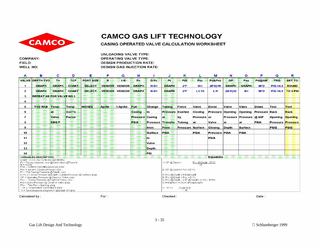
3 - 35Gas Lift Design And Technology Schlumberger 1999
6-1
Gas Lift Design And Technology Schlumberger 1999
GAS LIFT DESIGN AND TECHNOLOGY
6. Optimization
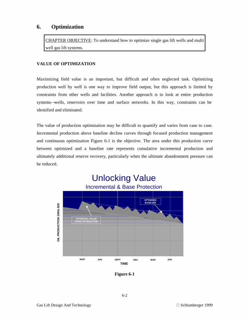
6-2
Gas Lift Design And Technology Schlumberger 1999
6. Optimization
CHAPTER OBJECTIVE: To understand how to optimize single gas lift wells and multi
well gas lift systems.
VALUE OF OPTIMIZATION
Maximizing field value is an important, but difficult and often neglected task. Optimizing
production well by well is one way to improve field output, but this approach is limited by
constraints from other wells and facilities. Another approach is to look at entire production
systems—wells, reservoirs over time and surface networks. In this way, constraints can be
identified and eliminated.
The value of production optimization may be difficult to quantify and varies from case to case.
Incremental production above baseline decline curves through focused production management
and continuous optimization Figure 6-1 is the objective. The area under this production curve
between optimized and a baseline rate represents cumulative incremental production and
ultimately additional reserve recovery, particularly when the ultimate abandonment pressure can
be reduced.
Figure 6-1
Unlocking ValueIncremental & Base Protection
OIL
PR
OD
UC
TIO
N 1
000s
B/D
TIME
MAR JUN SEPT DEC MAR JUN
OPTIMISEDBASELINE
POTENTIAL VALUEFROM OPTIMISATION
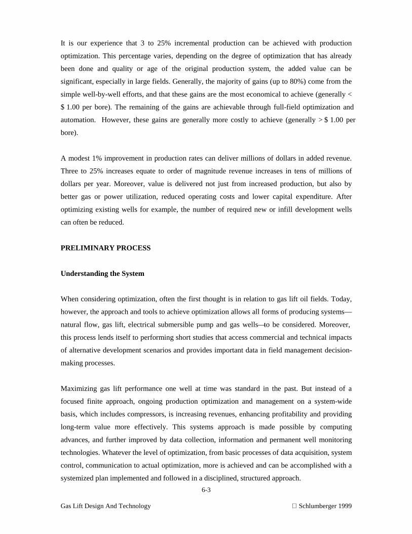
6-3
Gas Lift Design And Technology Schlumberger 1999
It is our experience that 3 to 25% incremental production can be achieved with production
optimization. This percentage varies, depending on the degree of optimization that has already
been done and quality or age of the original production system, the added value can be
significant, especially in large fields. Generally, the majority of gains (up to 80%) come from the
simple well-by-well efforts, and that these gains are the most economical to achieve (generally <
$1.00 per bore). The remaining of the gains are achievable through full-field optimization and
automation. However, these gains are generally more costly to achieve (generally >$1.00 per
bore).
A modest 1% improvement in production rates can deliver millions of dollars in added revenue.
Three to 25% increases equate to order of magnitude revenue increases in tens of millions of
dollars per year. Moreover, value is delivered not just from increased production, but also by
better gas or power utilization, reduced operating costs and lower capital expenditure. After
optimizing existing wells for example, the number of required new or infill development wells
can often be reduced.
PRELIMINARY PROCESS
Understanding the System
When considering optimization, often the first thought is in relation to gas lift oil fields. Today,
however, the approach and tools to achieve optimization allows all forms of producing systems—
natural flow, gas lift, electrical submersible pump and gas wells—to be considered. Moreover,
this process lends itself to performing short studies that access commercial and technical impacts
of alternative development scenarios and provides important data in field management decision-
making processes.
Maximizing gas lift performance one well at time was standard in the past. But instead of a
focused finite approach, ongoing production optimization and management on a system-wide
basis, which includes compressors, is increasing revenues, enhancing profitability and providing
long-term value more effectively. This systems approach is made possible by computing
advances, and further improved by data collection, information and permanent well monitoring
technologies. Whatever the level of optimization, from basic processes of data acquisition, system
control, communication to actual optimization, more is achieved and can be accomplished with a
systemized plan implemented and followed in a disciplined, structured approach.
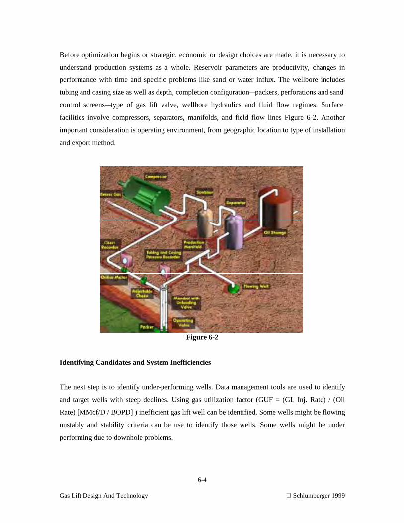
6-4
Gas Lift Design And Technology Schlumberger 1999
Before optimization begins or strategic, economic or design choices are made, it is necessary to
understand production systems as a whole. Reservoir parameters are productivity, changes in
performance with time and specific problems like sand or water influx. The wellbore includes
tubing and casing size as well as depth, completion configuration—packers, perforations and sand
control screens—type of gas lift valve, wellbore hydraulics and fluid flow regimes. Surface
facilities involve compressors, separators, manifolds, and field flow lines Figure 6-2. Another
important consideration is operating environment, from geographic location to type of installation
and export method.
Figure 6-2
Identifying Candidates and System Inefficiencies
The next step is to identify under-performing wells. Data management tools are used to identify
and target wells with steep declines. Using gas utilization factor (GUF = (GL Inj. Rate) / (Oil
Rate) [MMcf/D / BOPD] ) inefficient gas lift well can be identified. Some wells might be flowing
unstably and stability criteria can be use to identify those wells. Some wells might be under
performing due to downhole problems.
6-5
Gas Lift Design And Technology Schlumberger 1999
Poor production performance can also be contributed by system inefficiencies. Evaluating
gathering system and facilities is necessary to identify inefficiencies. Pressure restrictions in
flowlines are to be identified and eliminated. Thorough understanding about limitations of the
facilities –water handling capacity, oil handling capacity, gas compression capacity, gas sales
and/or dehydration capacity, lowest possible LP (low pressure) system pressure, gas sales
pressure and gaslift gas pressure & volumes available— aids in determining the maximum
production rate of the field at acceptable cost.
WELL-BY-WELL OPTIMIZATION
Data
Well-by-well optimization is prioritized to under-performing wells. It’s important to
understanding the well’s flowing condition by obtaining accurate single-rate or multi-rate well
tests using 2-pen recorders Figure 6-3 to measure tubing and casing pressures throughout test.
Where SCADA (System Control and Data Acquisition) is available, the need to collect 2-pen
charts is eliminated, as both this information and additional real-time information (manifold
pressures, etc.) is available at remote locations. These tools aid in understanding well
performance characteristics, as well as identifying, analyzing, and troubleshooting problems.
Figure 6-3
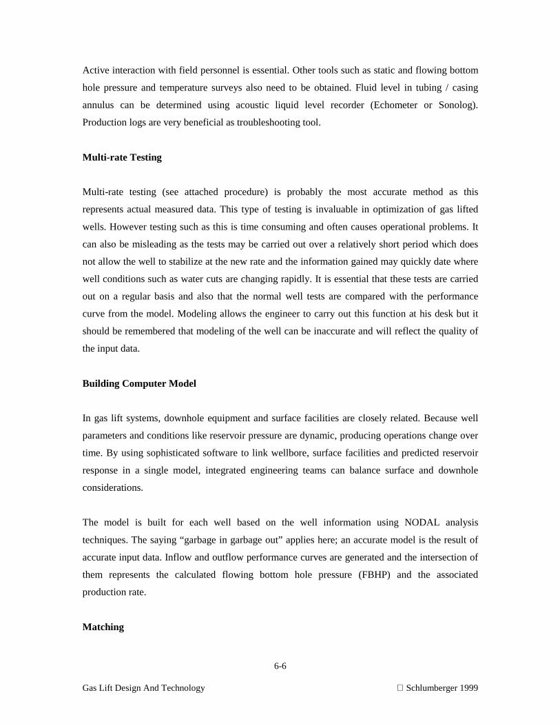
6-6
Gas Lift Design And Technology Schlumberger 1999
Active interaction with field personnel is essential. Other tools such as static and flowing bottom
hole pressure and temperature surveys also need to be obtained. Fluid level in tubing / casing
annulus can be determined using acoustic liquid level recorder (Echometer or Sonolog).
Production logs are very beneficial as troubleshooting tool.
Multi-rate Testing
Multi-rate testing (see attached procedure) is probably the most accurate method as this
represents actual measured data. This type of testing is invaluable in optimization of gas lifted
wells. However testing such as this is time consuming and often causes operational problems. It
can also be misleading as the tests may be carried out over a relatively short period which does
not allow the well to stabilize at the new rate and the information gained may quickly date where
well conditions such as water cuts are changing rapidly. It is essential that these tests are carried
out on a regular basis and also that the normal well tests are compared with the performance
curve from the model. Modeling allows the engineer to carry out this function at his desk but it
should be remembered that modeling of the well can be inaccurate and will reflect the quality of
the input data.
Building Computer Model
In gas lift systems, downhole equipment and surface facilities are closely related. Because well
parameters and conditions like reservoir pressure are dynamic, producing operations change over
time. By using sophisticated software to link wellbore, surface facilities and predicted reservoir
response in a single model, integrated engineering teams can balance surface and downhole
considerations.
The model is built for each well based on the well information using NODAL analysis
techniques. The saying “garbage in garbage out” applies here; an accurate model is the result of
accurate input data. Inflow and outflow performance curves are generated and the intersection of
them represents the calculated flowing bottom hole pressure (FBHP) and the associated
production rate.
Matching
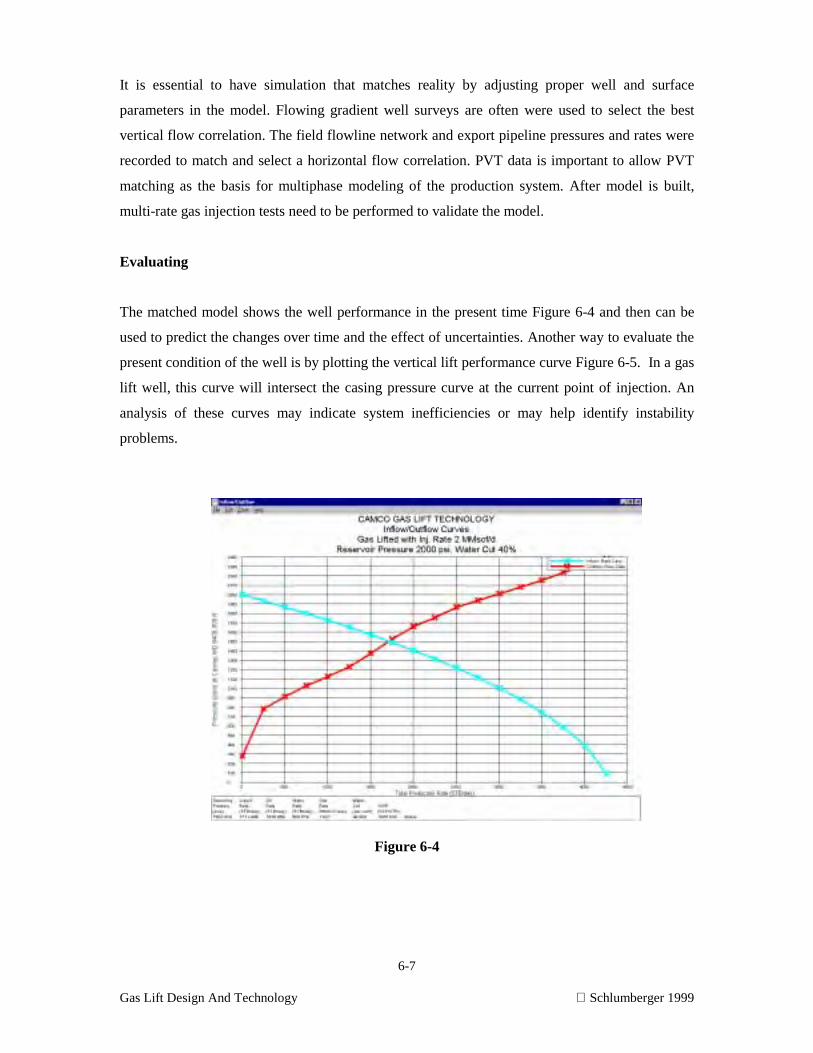
6-7
Gas Lift Design And Technology Schlumberger 1999
It is essential to have simulation that matches reality by adjusting proper well and surface
parameters in the model. Flowing gradient well surveys are often were used to select the best
vertical flow correlation. The field flowline network and export pipeline pressures and rates were
recorded to match and select a horizontal flow correlation. PVT data is important to allow PVT
matching as the basis for multiphase modeling of the production system. After model is built,
multi-rate gas injection tests need to be performed to validate the model.
Evaluating
The matched model shows the well performance in the present time Figure 6-4 and then can be
used to predict the changes over time and the effect of uncertainties. Another way to evaluate the
present condition of the well is by plotting the vertical lift performance curve Figure 6-5. In a gas
lift well, this curve will intersect the casing pressure curve at the current point of injection. An
analysis of these curves may indicate system inefficiencies or may help identify instability
problems.
Figure 6-4
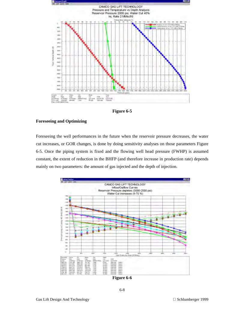
6-8
Gas Lift Design And Technology Schlumberger 1999
Figure 6-5
Foreseeing and Optimizing
Foreseeing the well performances in the future when the reservoir pressure decreases, the water
cut increases, or GOR changes, is done by doing sensitivity analyses on those parameters Figure
6-5. Once the piping system is fixed and the flowing well head pressure (FWHP) is assumed
constant, the extent of reduction in the BHFP (and therefore increase in production rate) depends
mainly on two parameters: the amount of gas injected and the depth of injection.
Figure 6-6
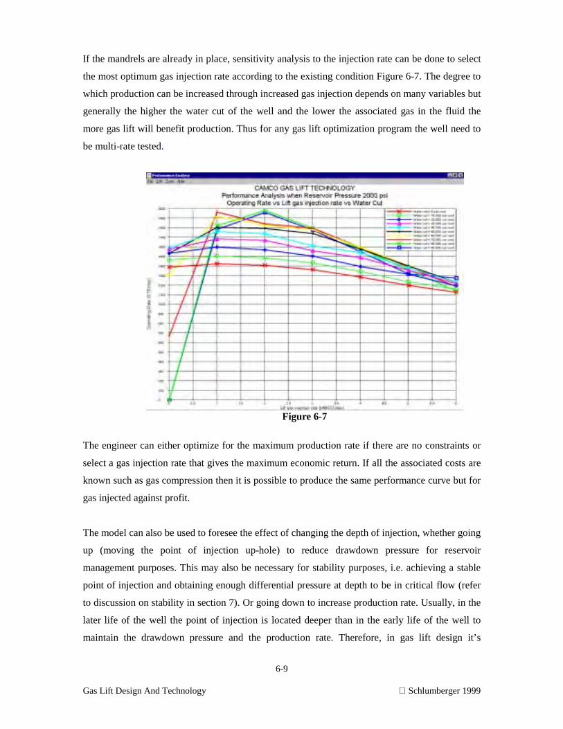
6-9
Gas Lift Design And Technology Schlumberger 1999
If the mandrels are already in place, sensitivity analysis to the injection rate can be done to select
the most optimum gas injection rate according to the existing condition Figure 6-7. The degree to
which production can be increased through increased gas injection depends on many variables but
generally the higher the water cut of the well and the lower the associated gas in the fluid the
more gas lift will benefit production. Thus for any gas lift optimization program the well need to
be multi-rate tested.
Figure 6-7
The engineer can either optimize for the maximum production rate if there are no constraints or
select a gas injection rate that gives the maximum economic return. If all the associated costs are
known such as gas compression then it is possible to produce the same performance curve but for
gas injected against profit.
The model can also be used to foresee the effect of changing the depth of injection, whether going
up (moving the point of injection up-hole) to reduce drawdown pressure for reservoir
management purposes. This may also be necessary for stability purposes, i.e. achieving a stable
point of injection and obtaining enough differential pressure at depth to be in critical flow (refer
to discussion on stability in section 7). Or going down to increase production rate. Usually, in the
later life of the well the point of injection is located deeper than in the early life of the well to
maintain the drawdown pressure and the production rate. Therefore, in gas lift design it’s
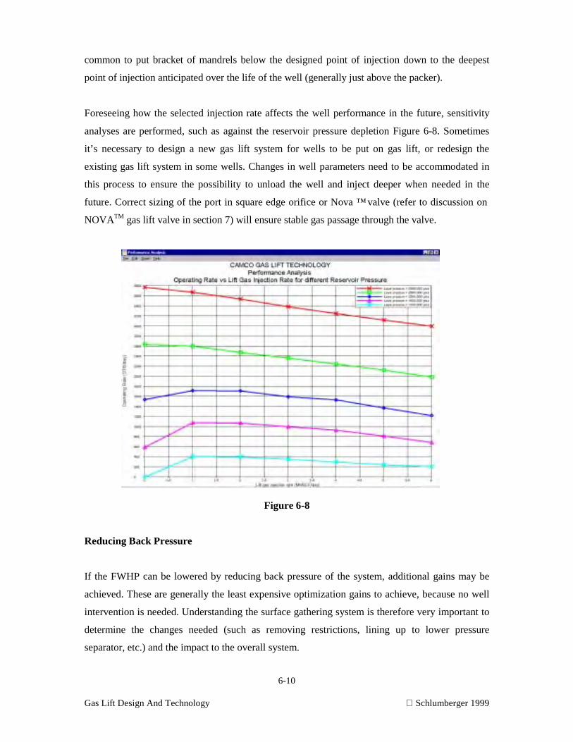
6-10
Gas Lift Design And Technology Schlumberger 1999
common to put bracket of mandrels below the designed point of injection down to the deepest
point of injection anticipated over the life of the well (generally just above the packer).
Foreseeing how the selected injection rate affects the well performance in the future, sensitivity
analyses are performed, such as against the reservoir pressure depletion Figure 6-8. Sometimes
it’s necessary to design a new gas lift system for wells to be put on gas lift, or redesign the
existing gas lift system in some wells. Changes in well parameters need to be accommodated in
this process to ensure the possibility to unload the well and inject deeper when needed in the
future. Correct sizing of the port in square edge orifice or Nova ™ valve (refer to discussion on
NOVATM gas lift valve in section 7) will ensure stable gas passage through the valve.
Figure 6-8
Reducing Back Pressure
If the FWHP can be lowered by reducing back pressure of the system, additional gains may be
achieved. These are generally the least expensive optimization gains to achieve, because no well
intervention is needed. Understanding the surface gathering system is therefore very important to
determine the changes needed (such as removing restrictions, lining up to lower pressure
separator, etc.) and the impact to the overall system.
6-11
Gas Lift Design And Technology Schlumberger 1999
Executing
The analysis process comes out with a list of works to execute, such as adjusting gas injection
rate, wireline intervention to change valves, etc. Interaction with field personnel is needed to
ensure all the works are done correctly.
FIELD-WIDE OPTIMIZATION
Field optimization would be fairly simple if there were no constraints in the system as the aim
would be to produce at the top of the curve. But it must be remembered that it is possible to over-
inject or restrict fluid production through injecting too much gas. However most fields are either
constrained by the available quantity of gas for injection or by the amount of fluid and gas that
can be processed through surface facilities. When this situation is encountered, optimization
becomes a much more complicated procedure as the return from each well will differ for the same
quantity of gas injected. The problem of field optimization has now been simplified with the
availability of allocation software.
Building the Model
For field-wide optimization it is necessary to have a field-wide model. Individual well models
generated before, together with data of compressors, separators, manifold, flowline network, and
export pipelines are used to build networked full-system model Figure 6-9. Once the basic full-
field model is built, all of the chokes, flowline dimensions, roughness and horizontal flow
correlations are then modified to ensure that the pressure drops that are estimated by the
simulation match those seen in reality.
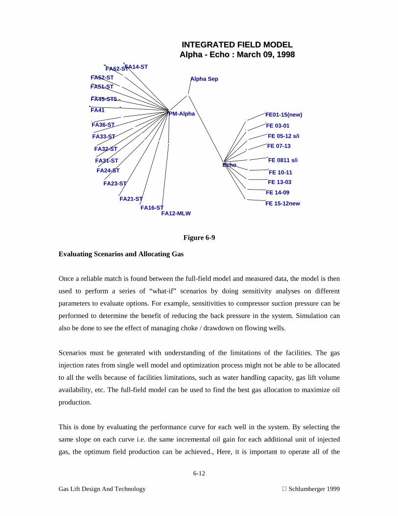
6-12
Gas Lift Design And Technology Schlumberger 1999
Figure 6-9
Evaluating Scenarios and Allocating Gas
Once a reliable match is found between the full-field model and measured data, the model is then
used to perform a series of “what-if” scenarios by doing sensitivity analyses on different
parameters to evaluate options. For example, sensitivities to compressor suction pressure can be
performed to determine the benefit of reducing the back pressure in the system. Simulation can
also be done to see the effect of managing choke / drawdown on flowing wells.
Scenarios must be generated with understanding of the limitations of the facilities. The gas
injection rates from single well model and optimization process might not be able to be allocated
to all the wells because of facilities limitations, such as water handling capacity, gas lift volume
availability, etc. The full-field model can be used to find the best gas allocation to maximize oil
production.
This is done by evaluating the performance curve for each well in the system. By selecting the
same slope on each curve i.e. the same incremental oil gain for each additional unit of injected
gas, the optimum field production can be achieved., Here, it is important to operate all of the
INTEGRATED FIELD MODELINTEGRATED FIELD MODELAlpha - Echo : March 09, 1998Alpha - Echo : March 09, 1998
Alpha Sep
PM-Alpha
FA52-ST
FA51-ST
FA45-ST5
FA41
FA36-ST
FA33-ST
FA32-ST
FA31-ST
FA24-ST
FA23-ST
FA21-ST
FA16-ST
FA14-ST
FA12-MLW
FA62-ST
Echo
FE 15-12new
FE 14-09
FE 13-03
FE 10-11
FE 0811 s/i
FE 07-13
FE 05-12 s/i
FE 03-01
FE01-15(new)
6-13
Gas Lift Design And Technology Schlumberger 1999
wells at the same injection pressure. This is necessary to prevent multi-point injection / instability
problems in adjacent wells.
Whilst this can be done by hand it is an extremely time consuming procedure and where gas
availability, process constraints and well performance curves may be constantly changing it is
almost impossible to maintain. With full-field model changes can be quickly evaluated and new
gas rates set. This operation can be taken a step further and fully automated.
Sometimes it’s necessary to do well stimulation or water shut-offs / conformance control to
enhance well performance. Well and full-field models can be used to screen and prioritize
candidates by predicting the benefit of those works to enhance production performance.
In some cases, several wells are fed with gas from compressor through a single gas line. In such
instance, it is difficult to provide the right volume of lift gas to each well. Even though the well is
equipped with choke, finding the right choke size is not an easy task. This problem is simplified
by having the full-field model, which helps in calculating the right choke size for each of the
well.
Maintaining the Model
The most important item to remember about optimization is that it is a continual process requiring
maintenance of models by doing regular scrutiny of surface data and well test information. Thus
the operator can be pro-active in maintaining his optimum production at all times both through
gas allocation and also through the early identification of problem and under-performing wells.
The result of optimization work is evaluated by comparing the predicted results to the actual
results. Performance is measured based on pre-determined criteria. Often the actual results are
still far from the prediction. Appropriate adjustments are made and the process is repeated. This is
a closed loop optimization process.
SUMMARY
In general, over the productive life of a field, optimization includes:
• well & field modeling and monitoring,
• data acquisition and management,
6-14
Gas Lift Design And Technology Schlumberger 1999
• continuous liaison contact with the onshore and offshore personnel to monitor the well
performance
• reconciling model predictions with measured data
• updating recommendations regularly for gas injection rates to ensure full field optimization
• training for both onshore and offshore staff to ensure a high level of gas lift awareness
amongst operations staff
• regular reporting of actual performance against targets
• equipment tracking (for reliable database)
• and equipment or system redesign if necessary
6-15
Gas Lift Design And Technology Schlumberger 1999
GENERAL PROCEDURES
FOR SINGLE OR MULTIRATE TESTING OF GAS LIFT WELLS
1. Before Test
• Check all surface gas injection facilities function and are calibrated correctly.
• Check there is full gas pressure from compressor.
• Ensure choke of well to be tested is fully open.
Note: Choke must be fully open at all times and never altered during testing.
• Connect chart recorders to the tubing and gas injection string at the wellhead. Tubing and
annulus pressure to be recorded for duration of test.
The following information is required:
• Test Separator Pressure & Temperature
• Oil and Gas Flow Rates from Test Separator
• WHFP / gage on tree
• WHFT
• Gas Injection Rate
• Gas Injection Pressure to Injection Header
• Gas Injection Pressure to Well at Wellhead
• Discharge Pressure and Temperature at Gas Compressor
• Water-cuts
• Choke Setting
2. Flow Well to (Test) Separator
• Set the desired gas injection rate.
• Flow well in test separator until it is stable.
• Ideally the well should be given at least a 6-12 hours stabilizing period, depending on the
mechanical configuration of the well i.e. highly deviated, horizontal well, long flowline,
etc. This should be extended if there is any sign of instability.
• Record stabilizing period start and end time.
6-16
Gas Lift Design And Technology Schlumberger 1999
• During stabilizing period monitor flow rate and record every hour. Every half an hour if
well shows signs of instability.
• Monitor and record wellhead flowing pressure (WHFP).
• Record wellhead flowing temperature (WHFT).
• Record test separator pressure and temperature.
• In later part of stabilizing period take water-cut sample and record result.
3. Commence Test
Once well is considered to be stable commence test. Test period at each gas injection
rate should be at least 6 hours, preferably 12 -18 hours.
• Record test start and end time.
• Monitor gas injection rate. Record any change that occurs during stabilizing period.
• Do not adjust choke or gas injection rate.
• If a chart can be connected to continuously record gas injection rate then do so.
• Record liquid flow rate from test separator every hour.
• Record gas flow rate from test separator every hour.
• Record totaliser readings at the start and at each hour of test
• Throughout test monitor separator pressure and temperature and note any changes.
• During test monitor separator pressure and temperature and note any changes.
• During test take water-cut sample and confirm this is consistent with earlier value.
• End test.
Note:
! Maximum injection rate is the maximum sustained gas rate which can be injected into the
well. This rate should be recorded.
! It is important that each well is tested and as good a spread of injection rates as possible
achieved.
7-1
Gas Lift Design And Technology Schlumberger 1999
GAS LIFT DESIGN AND TECHNOLOGY
7. Troubleshooting
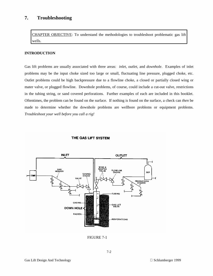
7-2
Gas Lift Design And Technology Schlumberger 1999
7. Troubleshooting
CHAPTER OBJECTIVE: To understand the methodologies to troubleshoot problematic gas lift
wells.
INTRODUCTION
Gas lift problems are usually associated with three areas: inlet, outlet, and downhole. Examples of inlet
problems may be the input choke sized too large or small, fluctuating line pressure, plugged choke, etc.
Outlet problems could be high backpressure due to a flowline choke, a closed or partially closed wing or
mater valve, or plugged flowline. Downhole problems, of course, could include a cut-out valve, restrictions
in the tubing string, or sand covered perforations. Further examples of each are included in this booklet.
Oftentimes, the problem can be found on the surface. If nothing is found on the surface, a check can then be
made to determine whether the downhole problems are wellbore problems or equipment problems.
Troubleshoot your well before you call a rig!
FIGURE 7-1
7-3
Gas Lift Design And Technology Schlumberger 1999
INLET PROBLEMS
Choke sized too large
Check for casing pressure at or above design operating pressure. This can cause reopening upper pressure
valves and/or excessive gas usage. Approximate gas usages for various flow rates are included in the section
on “tuning in” the well.
Choke sized too small
Check for reduced fluid production as a result of insufficient gas injection. This condition can sometimes
prevent the well from fully unloading. The design gas liquid ratio can often give an indication of the choke
size to use as a starting point.
Low casing pressure
This condition can occur due to the choke being sized too small or the choke being plugged or frozen up.
Choke freezing can often be eliminated by continuous injection of methanol in the gas lift gas. A check of
gas volume being injected will separate this case from low casing pressure due to a hole in the tubing or
cutout valve. Verify the gauge readings to be sure the problem is real.
High casing pressure
This condition can occur due to the choke being sized too large. Check for excessive gas usage due to
reopening upper pressure valves. If high-casing pressure is accompanied by low injection gas volumes, it is
possible that the operating valve may be partially plugged or high tubing pressure may be reducing the
differential between the tubing and casing. (Remove flowline choke and restriction). High casing pressure
accompanying low injection gas volumes may also be caused by higher than anticipated temperatures raising
the set pressures of pressure operated valves.
Verify gauges
Inaccurate gauges can cause false indications of high or low casing pressures. Always check the wellhead
casing and tubing pressures with a calibrated gauge.

7-4
Gas Lift Design And Technology Schlumberger 1999
Low gas volume
Check to insure that the gas lift line valve is fully open and that the casing choke is not too small, frozen or
plugged. Check to see if the available operating pressure is in the range required to open the valves. Be sure
that the gas volume is being delivered to the well, as nearby wells may be robbing the system - especially
intermittent wells. Sometimes a higher than anticipated producing rate and the resulting higher temperature
will cause the valve set pressure to increase and thereby restrict the gas input.
Excessive gas volume
This condition can be caused by the casing choke sized too large or excessive casing pressure. Check to see
if the casing pressure is above the design pressure causing upper pressure valves to be open. A tubing leak
or cut-out valve can also cause this symptom but they will generally also cause a low casing pressure.
7-5
Gas Lift Design And Technology Schlumberger 1999
OUTLET PROBLEMS
Valve restrictions
Check to insure that all valves at the tree and header are fully open or that an undersized valve is not in the
line (i.e. 1-inch valve in 2-inch flowline). Other restrictions may result from a smashed or crimped flowline.
For example, check places where the line crosses a road.
High back pressure
Wellhead pressure is transmitted to the bottom of the hole, reducing the differential into the wellbore and
thereby reducing production. Check to insure that no choke is in the flowline. Even with no choke bean in a
choke body, it is usually restricted to less than full I.D. Remove the choke body if possible. Excessive 90o
turns can cause high back pressure and should be removed where feasible. High backpressure can also result
from paraffin or scale buildup in the flowline. Hot oiling the line will generally remove paraffin. However,
scale may or may not be able to be removed depending on the type. Where high backpressure is due to long
flowlines, it may be possible to reduce the pressure by “looping” the flowline with an inactive line. The
same would apply to cases where the flowline I.D. is smaller than the tubing I.D. Sometimes a partially open
check valve in the flowline can cause excessive backpressure. Common flowlines can cause excessive
backpressure and should be avoided if possible. Check all possibilities and remove as many restrictions from
the system as possible.
Separator operating pressure
The separator pressure should be maintained as low as possible for gas lift wells. Often a well may be
flowing to a high or intermediate pressure system when it dies and is placed on gas lift. Insure that the well
is switched to the lowest pressure system available. Sometimes an undersized orifice plate in the meter at the
separator will cause high backpressure.
7-6
Gas Lift Design And Technology Schlumberger 1999
DOWNHOLE PROBLEMS
Hole in tubing
Indicators of a hole in the tubing include abnormally low casing pressure and excess gas usage. A hole in the
tubing can be confirmed by the following procedure: Equalize the tubing pressure and casing pressure by
closing the wing valve with the gas lift gas on. After the pressures are equalized, shut off the gas input valve
and rapidly bleed-off the casing pressure. If the tubing pressure bleeds as the casing pressure drops, then a
hole is indicated. The tubing pressure will hold if no hole is present since both the check valves and gas lift
valves will be in the closed position as the casing pressure bleeds to zero. A packer leak may also cause
symptoms similar to a hole in the tubing.
Operating pressure valve by surface closing pressure method
A pressure-operated valve will pass gas until the casing pressure drops to the closing pressure of the valve.
As a result, the operating valve can often be estimated by shutting off the input gas and observing the
pressure at which the casing holds. This pressure is the surface closing pressure of the operating valve.
Closing pressure analysis assumes the tubing pressure to be zero, and single point injection. These
assumptions limit the accuracy of this method since the tubing pressure at each valve is never zero, and
multipoint injection may be occurring. This method can be useful when used in combination with other data
to bracket the operating valve.
Well blowing dry gas
For pressure valves, check to insure that the casing pressure is not in excess of the design operating pressure,
thereby causing operating from the upper valves. Insure that no hole exists in the tubing by the previously
mentioned method. If the upper valves are not being held open by excess casing pressure and no hole exists,
then operation is probably from the bottom valve. Additional verification can be obtained by checking the
surface closing pressure as indicated above. In the case where the well is equipped with fluid valves and a
pressure valve on the bottom, blowing dry gas is a positive indication of operation from the bottom valve
after the possibility of a hole in the tubing has been eliminated. Operation from the bottom valve generally
indicates a lack of feed-in. Often it is advisable to tag bottom with wireline tools to see if the perforations
have been covered by sand. When the well is equipped with a standing valve, check to insure the standing
valve is not stuck in the closed position.
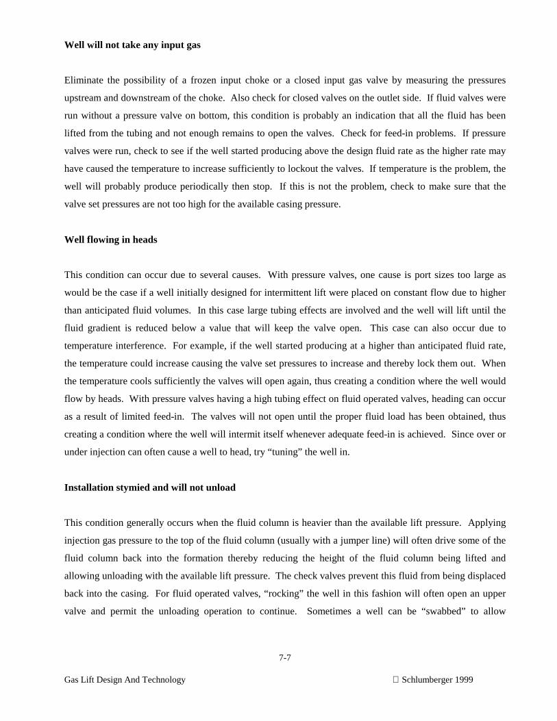
7-7
Gas Lift Design And Technology Schlumberger 1999
Well will not take any input gas
Eliminate the possibility of a frozen input choke or a closed input gas valve by measuring the pressures
upstream and downstream of the choke. Also check for closed valves on the outlet side. If fluid valves were
run without a pressure valve on bottom, this condition is probably an indication that all the fluid has been
lifted from the tubing and not enough remains to open the valves. Check for feed-in problems. If pressure
valves were run, check to see if the well started producing above the design fluid rate as the higher rate may
have caused the temperature to increase sufficiently to lockout the valves. If temperature is the problem, the
well will probably produce periodically then stop. If this is not the problem, check to make sure that the
valve set pressures are not too high for the available casing pressure.
Well flowing in heads
This condition can occur due to several causes. With pressure valves, one cause is port sizes too large as
would be the case if a well initially designed for intermittent lift were placed on constant flow due to higher
than anticipated fluid volumes. In this case large tubing effects are involved and the well will lift until the
fluid gradient is reduced below a value that will keep the valve open. This case can also occur due to
temperature interference. For example, if the well started producing at a higher than anticipated fluid rate,
the temperature could increase causing the valve set pressures to increase and thereby lock them out. When
the temperature cools sufficiently the valves will open again, thus creating a condition where the well would
flow by heads. With pressure valves having a high tubing effect on fluid operated valves, heading can occur
as a result of limited feed-in. The valves will not open until the proper fluid load has been obtained, thus
creating a condition where the well will intermit itself whenever adequate feed-in is achieved. Since over or
under injection can often cause a well to head, try “tuning” the well in.
Installation stymied and will not unload
This condition generally occurs when the fluid column is heavier than the available lift pressure. Applying
injection gas pressure to the top of the fluid column (usually with a jumper line) will often drive some of the
fluid column back into the formation thereby reducing the height of the fluid column being lifted and
allowing unloading with the available lift pressure. The check valves prevent this fluid from being displaced
back into the casing. For fluid operated valves, “rocking” the well in this fashion will often open an upper
valve and permit the unloading operation to continue. Sometimes a well can be “swabbed” to allow
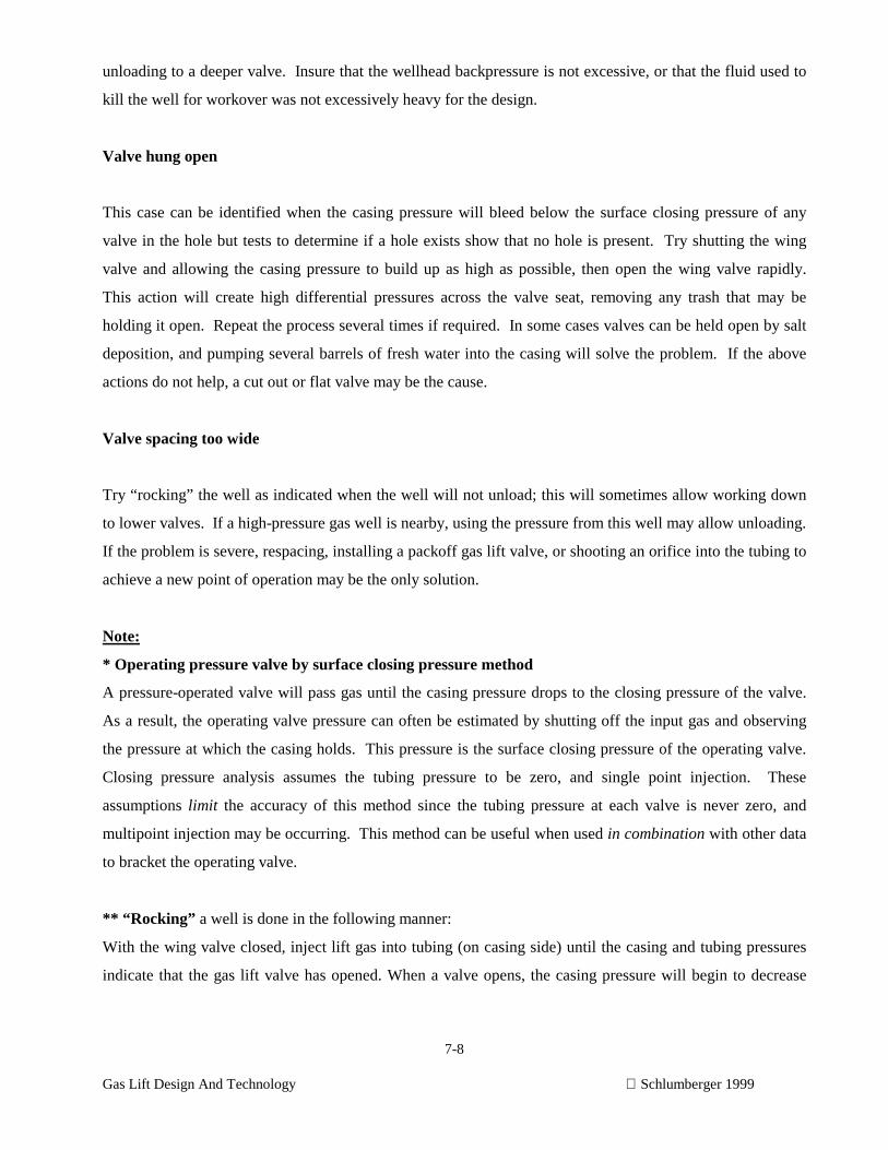
7-8
Gas Lift Design And Technology Schlumberger 1999
unloading to a deeper valve. Insure that the wellhead backpressure is not excessive, or that the fluid used to
kill the well for workover was not excessively heavy for the design.
Valve hung open
This case can be identified when the casing pressure will bleed below the surface closing pressure of any
valve in the hole but tests to determine if a hole exists show that no hole is present. Try shutting the wing
valve and allowing the casing pressure to build up as high as possible, then open the wing valve rapidly.
This action will create high differential pressures across the valve seat, removing any trash that may be
holding it open. Repeat the process several times if required. In some cases valves can be held open by salt
deposition, and pumping several barrels of fresh water into the casing will solve the problem. If the above
actions do not help, a cut out or flat valve may be the cause.
Valve spacing too wide
Try “rocking” the well as indicated when the well will not unload; this will sometimes allow working down
to lower valves. If a high-pressure gas well is nearby, using the pressure from this well may allow unloading.
If the problem is severe, respacing, installing a packoff gas lift valve, or shooting an orifice into the tubing to
achieve a new point of operation may be the only solution.
Note:
* Operating pressure valve by surface closing pressure method
A pressure-operated valve will pass gas until the casing pressure drops to the closing pressure of the valve.
As a result, the operating valve pressure can often be estimated by shutting off the input gas and observing
the pressure at which the casing holds. This pressure is the surface closing pressure of the operating valve.
Closing pressure analysis assumes the tubing pressure to be zero, and single point injection. These
assumptions limit the accuracy of this method since the tubing pressure at each valve is never zero, and
multipoint injection may be occurring. This method can be useful when used in combination with other data
to bracket the operating valve.
** “Rocking” a well is done in the following manner:
With the wing valve closed, inject lift gas into tubing (on casing side) until the casing and tubing pressures
indicate that the gas lift valve has opened. When a valve opens, the casing pressure will begin to decrease
7-9
Gas Lift Design And Technology Schlumberger 1999
and to equalize with the tubing pressure. The tubing pressure also should begin to increase at a faster rate
with injection gas entering the tubing through the valve and surface connection.
Stop the gas injection into the tubing and open the wing valve to lift the liquid slug above the valve into the
flowline as rapidly as possible. A flowline choke may be required to prevent venting injection gas through
the separator relief valve. Some surface facilities are overloaded easily and bleeding the tubing pressure must
be controlled carefully. The rocking process may be required several times until a lower gas lift valve has
been uncovered.
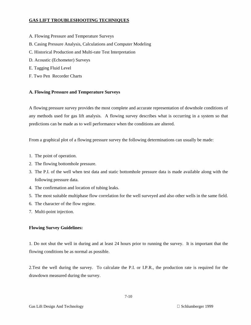
7-10
Gas Lift Design And Technology Schlumberger 1999
GAS LIFT TROUBLESHOOTING TECHNIQUES
A. Flowing Pressure and Temperature Surveys
B. Casing Pressure Analysis, Calculations and Computer Modeling
C. Historical Production and Multi-rate Test Interpretation
D. Acoustic (Echometer) Surveys
E. Tagging Fluid Level
F. Two Pen Recorder Charts
A. Flowing Pressure and Temperature Surveys
A flowing pressure survey provides the most complete and accurate representation of downhole conditions of
any methods used for gas lift analysis. A flowing survey describes what is occurring in a system so that
predictions can be made as to well performance when the conditions are altered.
From a graphical plot of a flowing pressure survey the following determinations can usually be made:
1. The point of operation.
2. The flowing bottomhole pressure.
3. The P.I. of the well when test data and static bottomhole pressure data is made available along with the
following pressure data.
4. The confirmation and location of tubing leaks.
5. The most suitable multiphase flow correlation for the well surveyed and also other wells in the same field.
6. The character of the flow regime.
7. Multi-point injection.
Flowing Survey Guidelines:
1. Do not shut the well in during and at least 24 hours prior to running the survey. It is important that the
flowing conditions be as normal as possible.
2.Test the well during the survey. To calculate the P.I. or I.P.R., the production rate is required for the
drawdown measured during the survey.
7-11
Gas Lift Design And Technology Schlumberger 1999
3.If a tubing leak is suspected, at least one stop should be made between each gas lift valve and additional
stops made in the area of the suspected leak.
4.The use of small diameter pressure instruments will minimize the restriction to flow and reduce the forces
acting to “blow the tools up the hole”.
5. If the well is being entered under flowing conditions, it is important to keep the tools from being “blown
up the hole”. In addition to using small diameter bombs, weighted stem and “no-flow latches” should be
used. Upward movement of the tool string activates a set of slips in the no-flow latch to prevent being
“blown up the hole”.
6. Running tandem pressure instruments can save valuable time, effort and money by providing a backup for
the event of a miss-run with the No. 1 instrument.
7. Running a flowing temperature survey in conjunction with flowing pressure surveys can often provide
very useful information. Temperature surveys can identify problems caused by miscalculations of test rack
opening pressure due to erroneous temperature data and leaking gas lift valves or tubing can sometimes be
located or confirmed with temperature surveys. When running a temperature survey, it is a good practice to
make a stop below the mud line in addition to the stop in the lubricator for offshore wells and several
hundred feed below the surface for wells in arctic or near arctic areas so that a more accurate flowing
geothermal gradient can be determined.
If it is not possible to run a temperature instrument, at the very least, a temperature measurement with a
maximum recording thermometer should be obtained.
8.For mechanical pressure instruments it is recommended that the maximum anticipated pressure in the well
not exceed 75 percent of the maximum pressure of the instrument.
9.In general, it is better to use the fastest clock possible to drive the chart and still provide the time required
to run the survey.
7-12
Gas Lift Design And Technology Schlumberger 1999
Plotting Survey Results:
The results of flowing pressure surveys are plotted on graph paper, along with other wellhead pressure data,
to produce gradient curves. The plotted gradients allow visual interpretation of all the data.
Procedures for Running Flowing Pressure Surveys:
Continuous flow gas lift wells:
1. Flow the well to a test separator for 24 hours to obtain a stabilized producing rate. (Test facilities should
duplicate as nearly as possible normal production facilities).
2. Place well on test before running the bottomhole pressure. The test should be long enough to provide a
representative daily rate. The duration of the test depends largely on the stability of the flow rate.
3. Record the pressure in the lubricator for ten minutes. Obtain a pressure reading of the lubricator pressure
with a dead weight tester for comparison. Run the pressure bomb down the tubing, making stops
approximately 50 feet below each gas lift valve. (Do not shut the well in while rigging up or running the
survey).
4. The pressure instrument should remain at bottom stop for an interval double that of the other stops.
5. The casing pressure should be recorded with a dead weight tester or a calibrated two-pen recorder.
6.If a static BHP is to be recorded, shut off lift gas and close the flow line wing valve. Leave the pressure
instrument on bottom for time interval necessary for build-up. This could necessitate running two bombs in
tandem with clocks having different speeds.
7-13
Gas Lift Design And Technology Schlumberger 1999
B. Casing Pressure Analysis, Calculations and Computer Modeling
One method of checking gas lift performance is by calculating the operating valve. This can be
accomplished by calculating surface closing pressures or by comparing the valve opening pressures with the
opening forces that exist at each valve downhole due to the operating tubing and casing pressures,
temperatures, etc. Although this method may not be as accurate as a flowing pressure survey due to
inaccuracies in the data used, it can still be a valuable tool in high grading the well selection for more
expensive types of diagnostic methods.
C. Historical Well Production and Multi-rate Test Interpretation
A well test report for troubleshooting as referred to in this text will provide the following data:
1. Gross fluid production.
2. Water cut.
3. Oil production.
4. Tubing head pressure.
5. Casing head pressure.
6. Produced gas. (total)
7. Lift gas.
8. Gas liquid ratio.
9. Lift gas choke bean size.
10. Flowline choke bean size. (if applicable)
The well test should be of sufficient duration to provide a representative average daily producing rate. If a
well is very unstable, it may require a test period of more than 24 hours to obtain a representative average
24-hour rate. Flowing pressure/temperature surveys or casing/tubing pressure recordings should be made
during the well test period.
The well test conditions should duplicate as nearly as possible the normal producing conditions.
7-14
Gas Lift Design And Technology Schlumberger 1999
D. Acoustic (Echometer) Well Sounding Devices
The fluid level in the annulus of a gas lift well will sometimes give an indication of the depth of lift. This
method involves firing a cartridge at the surface and utilizes the principle of sound waves to determine the
depth of the fluid level in the annulus. Acoustic devices are fairly inexpensive when compared to flowing
pressure surveys. It should be noted that for wells with packers, it is possible for the well to have lifted
down to a deeper valve while unloading, then returned to operation at a valve up the hole. The resulting
fluid level in the annulus will be below the actual point of operation.
E. Tagging Fluid Level
Tagging the fluid level in a well with wireline tools can sometimes give an estimation of the operating valve
subject to several limitations. Fluid feed-in will often raise the fluid level before the wireline tools can get
down the hole. In addition, fluid fallback will always occur after the gas lift gas has been shut off. Both of
these factors will cause the observed fluid level to be above the operating valve. Care should be taken to
insure that the input gas valve was closed prior to closing the wing valve or the gas pressure will drive the
fluid back down the hole and below the point of operation. This is certainly a questionable method.
F. Two Pen Recorder Charts
In order to calculate the operating valve, it is necessary to have accurate tubing and casing pressure data.
Two pen recorder charts give a continuous recording of these pressures, and can be quite useful if
accompanied by an accurate well test. The two pen recorder charts can be used to optimize surface controls,
locate surface problems, as well as identify downhole problems.
7-15
Gas Lift Design And Technology Schlumberger 1999
WHERE TO INSTALL A 2-PEN RECORDER
Connect casing pen line
1. At well; not at compressor or gas distribution header.
2. Down stream of input choke so that the true surface casing pressure is recorded.
Connect tubing pen line
1. At the well; not at the battery, separator, or production header.
2. Upstream of choke body or other restrictions. (Even with no choke bean, less than full opening is
found in most chokes).
INTERPRETATION OF 2-PEN RECORDER CHARTS ON GAS LIFT WELLS
The two most significant forces acting on any gas lift valve are the tubing pressure and the casing pressure.
The downhole values can be calculated and compared to the operating characteristics of the type gas lift
valves in service. From this information it is possible to estimate the point of operation. Observing the
surface pressures can also give valuable information on the efficiency of the system. Charts illustrating the
type of information to be gained by the use of 2-pen recorders are included.
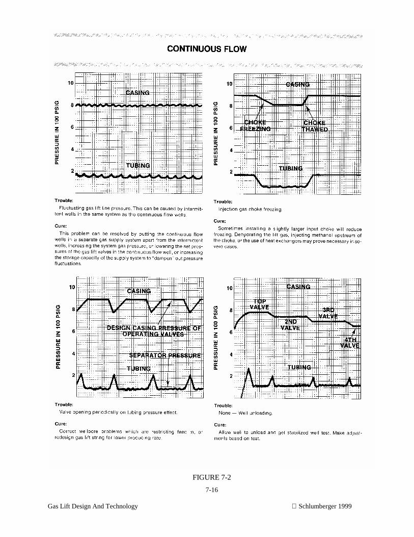
7-16
Gas Lift Design And Technology Schlumberger 1999
FIGURE 7-2
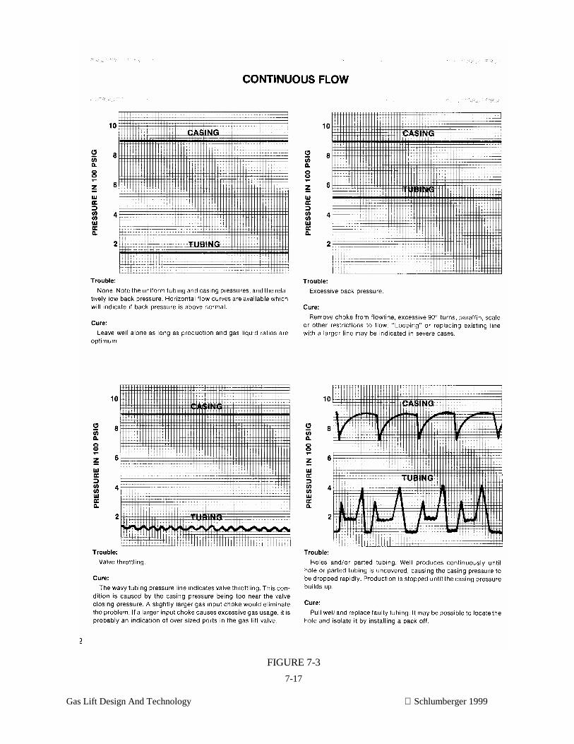
7-17
Gas Lift Design And Technology Schlumberger 1999
FIGURE 7-3
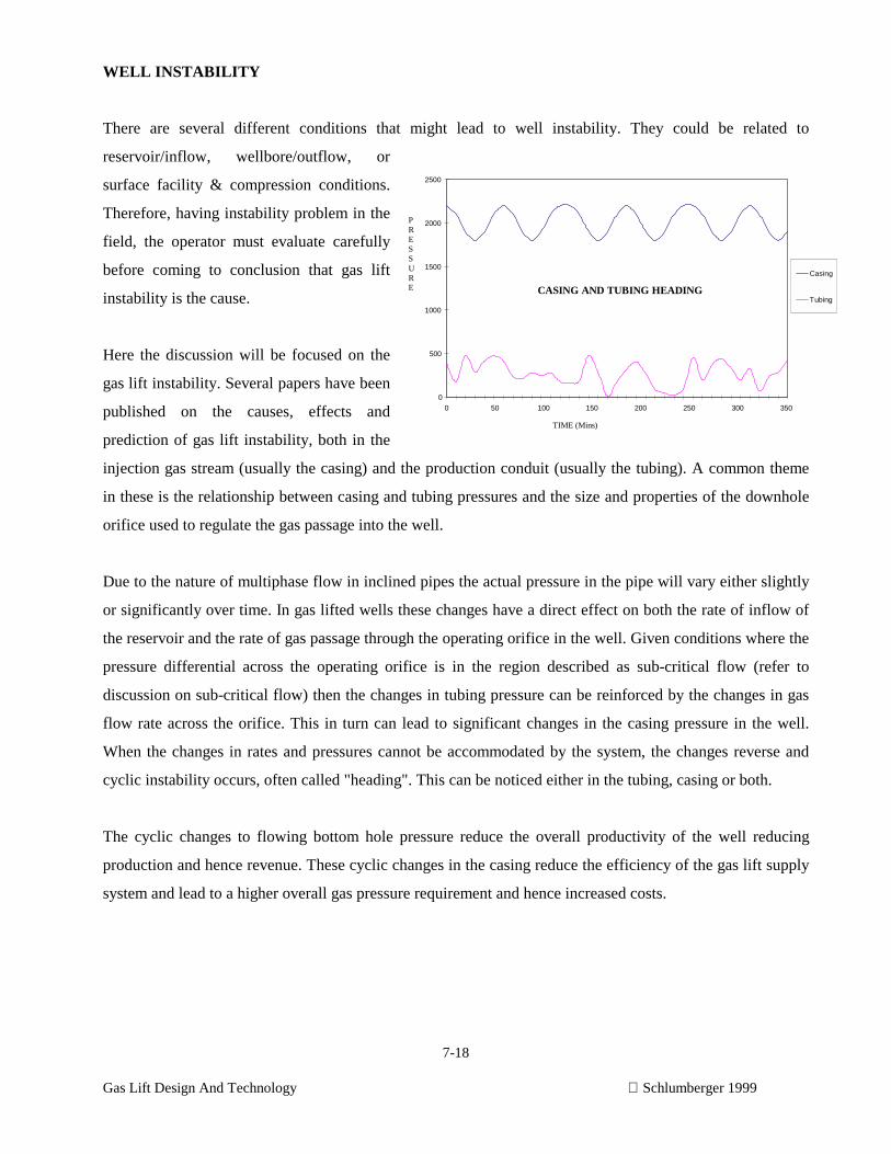
7-18
Gas Lift Design And Technology Schlumberger 1999
WELL INSTABILITY
There are several different conditions that might lead to well instability. They could be related to
reservoir/inflow, wellbore/outflow, or
surface facility & compression conditions.
Therefore, having instability problem in the
field, the operator must evaluate carefully
before coming to conclusion that gas lift
instability is the cause.
Here the discussion will be focused on the
gas lift instability. Several papers have been
published on the causes, effects and
prediction of gas lift instability, both in the
injection gas stream (usually the casing) and the production conduit (usually the tubing). A common theme
in these is the relationship between casing and tubing pressures and the size and properties of the downhole
orifice used to regulate the gas passage into the well.
Due to the nature of multiphase flow in inclined pipes the actual pressure in the pipe will vary either slightly
or significantly over time. In gas lifted wells these changes have a direct effect on both the rate of inflow of
the reservoir and the rate of gas passage through the operating orifice in the well. Given conditions where the
pressure differential across the operating orifice is in the region described as sub-critical flow (refer to
discussion on sub-critical flow) then the changes in tubing pressure can be reinforced by the changes in gas
flow rate across the orifice. This in turn can lead to significant changes in the casing pressure in the well.
When the changes in rates and pressures cannot be accommodated by the system, the changes reverse and
cyclic instability occurs, often called "heading". This can be noticed either in the tubing, casing or both.
The cyclic changes to flowing bottom hole pressure reduce the overall productivity of the well reducing
production and hence revenue. These cyclic changes in the casing reduce the efficiency of the gas lift supply
system and lead to a higher overall gas pressure requirement and hence increased costs.
0
500
1000
1500
2000
2500
0 50 100 150 200 250 300 350
Casing
Tubing
TIME (Mins)
PRESSURE CASING AND TUBING HEADING
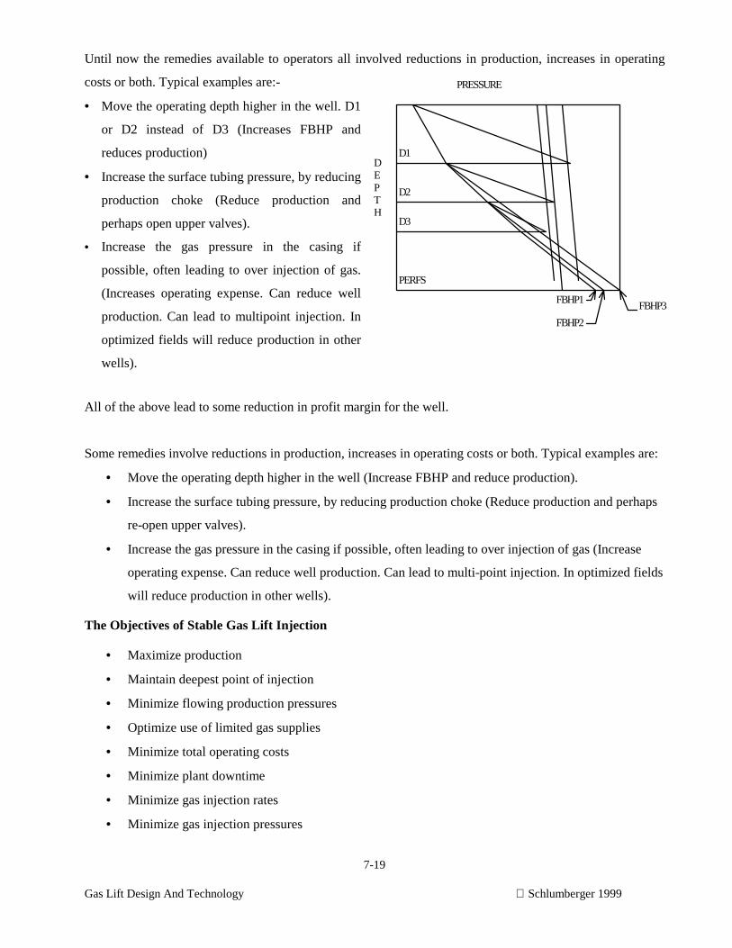
7-19
Gas Lift Design And Technology Schlumberger 1999
Until now the remedies available to operators all involved reductions in production, increases in operating
costs or both. Typical examples are:-
• Move the operating depth higher in the well. D1
or D2 instead of D3 (Increases FBHP and
reduces production)
• Increase the surface tubing pressure, by reducing
production choke (Reduce production and
perhaps open upper valves).
• Increase the gas pressure in the casing if
possible, often leading to over injection of gas.
(Increases operating expense. Can reduce well
production. Can lead to multipoint injection. In
optimized fields will reduce production in other
wells).
All of the above lead to some reduction in profit margin for the well.
Some remedies involve reductions in production, increases in operating costs or both. Typical examples are:
• Move the operating depth higher in the well (Increase FBHP and reduce production).
• Increase the surface tubing pressure, by reducing production choke (Reduce production and perhaps
re-open upper valves).
• Increase the gas pressure in the casing if possible, often leading to over injection of gas (Increase
operating expense. Can reduce well production. Can lead to multi-point injection. In optimized fields
will reduce production in other wells).
The Objectives of Stable Gas Lift Injection
• Maximize production
• Maintain deepest point of injection
• Minimize flowing production pressures
• Optimize use of limited gas supplies
• Minimize total operating costs
• Minimize plant downtime
• Minimize gas injection rates
• Minimize gas injection pressures
PRESSURE
DEPTH
FBHP1
FBHP2
D1
D2
D3
FBHP3
PERFS
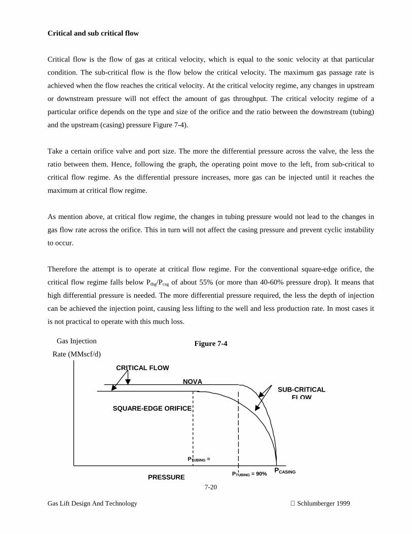
G
Critical and sub critical flow
Critical flow is the flow of gas at critical velocity, which is equal to the sonic velocity at that particular
condition. The sub-critical flow is the flow below the critical velocity. The maximum gas passage rate is
achieved when the flow reaches the critical velocity. At the critical velocity regime, any changes in upstream
or downstream pressure will not effect the amount of gas throughput. The critical velocity regime of a
particular orifice depends on the type and size of the orifice and the ratio between the downstream (tubing)
and the upstream (casing) pressure Figure 7-4).
Take a certain orifice valve and port size. The more the differential pressure across the valve, the less the
ratio between them. Hence, following the graph, the operating point move to the left, from sub-critical to
critical flow regime. As the differential pressure increases, more gas can be injected until it reaches the
maximum at critical flow regime.
As mention above, at critical flow regime, the changes in tubing pressure would not lead to the changes in
gas flow rate across the orifice. This in turn will not affect the casing pressure and prevent cyclic instability
to occur.
Therefore the attempt is to operate at critical flow regime. For the conventional square-edge orifice, the
critical flow regime falls below Ptbg/Pcsg of about 55% (or more than 40-60% pressure drop). It means that
high differential pressure is needed. The more differential pressure required, the less the depth of injection
can be achieved the injection point, causing less lifting to the well and less production rate. In most cases it
is not practical to operate with this much loss.
Figure 7-4
Gas InjectionRate (MMscf/d)
7-20
as Lift Design And Technology Schlumberger 1999
SUB-CRITICALFLOW
NOVA
PRESSUREPCASINGPTUBING = 90%
PTUBING =
SQUARE-EDGE ORIFICE
CRITICAL FLOW
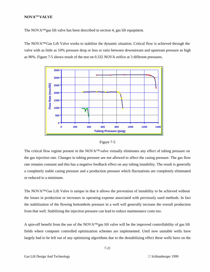
7-21
Gas Lift Design And Technology Schlumberger 1999
NOVATM VALVE
The NOVA™ gas lift valve has been described in section 4, gas lift equipment.
The NOVA™ Gas Lift Valve works to stabilize the dynamic situation. Critical flow is achieved through the
valve with as little as 10% pressure drop or less or ratio between downstream and upstream pressure as high
as 90%. Figure 7-5 shows result of the test on 0.332 NOVA orifice at 3 different pressures.
Figure 7-5
The critical flow regime present in the NOVA™ valve virtually eliminates any effect of tubing pressure on
the gas injection rate. Changes in tubing pressure are not allowed to affect the casing pressure. The gas flow
rate remains constant and this has a negative feedback effect on any tubing instability. The result is generally
a completely stable casing pressure and a production pressure which fluctuations are completely eliminated
or reduced to a minimum.
The NOVA™ Gas Lift Valve is unique in that it allows the prevention of instability to be achieved without
the losses in production or increases in operating expense associated with previously used methods. In fact
the stabilization of the flowing bottomhole pressure in a well will generally increase the overall production
from that well. Stabilizing the injection pressure can lead to reduce maintenance costs too.
A spin-off benefit from the use of the NOVA™ gas lift valve will be the improved controllability of gas lift
fields where computer controlled optimization schemes are implemented. Until now unstable wells have
largely had to be left out of any optimizing algorithms due to the destabilizing effect these wells have on the
0
500
1000
1500
2000
2500
3000
3500
0 200 400 600 800 1000 1200 1400
Tubing Pressure (psig)
Flo
w R
ate
(msc
f/D
)
0
500
1000
1500
2000
2500
3000
3500
0 200 400 600 800 1000 1200 1400
Tubing Pressure (psig)
Flo
w R
ate
(msc
f/D
)
7-22
Gas Lift Design And Technology Schlumberger 1999
measuring and feedback controls in such a system. With the NOVA™ gas lift valve even if a well is slightly
tubing unstable the gas rate will remain constant. Hence the gas measurement which is the control parameter
for these systems will remain stable. This should make it possible to include more wells than ever in
optimization schemes.
NOVA™ Gas Lift Valves and Dual Wells
Dual gas lift wells are discussed in Chapter 4, Gas Lift Equipment.
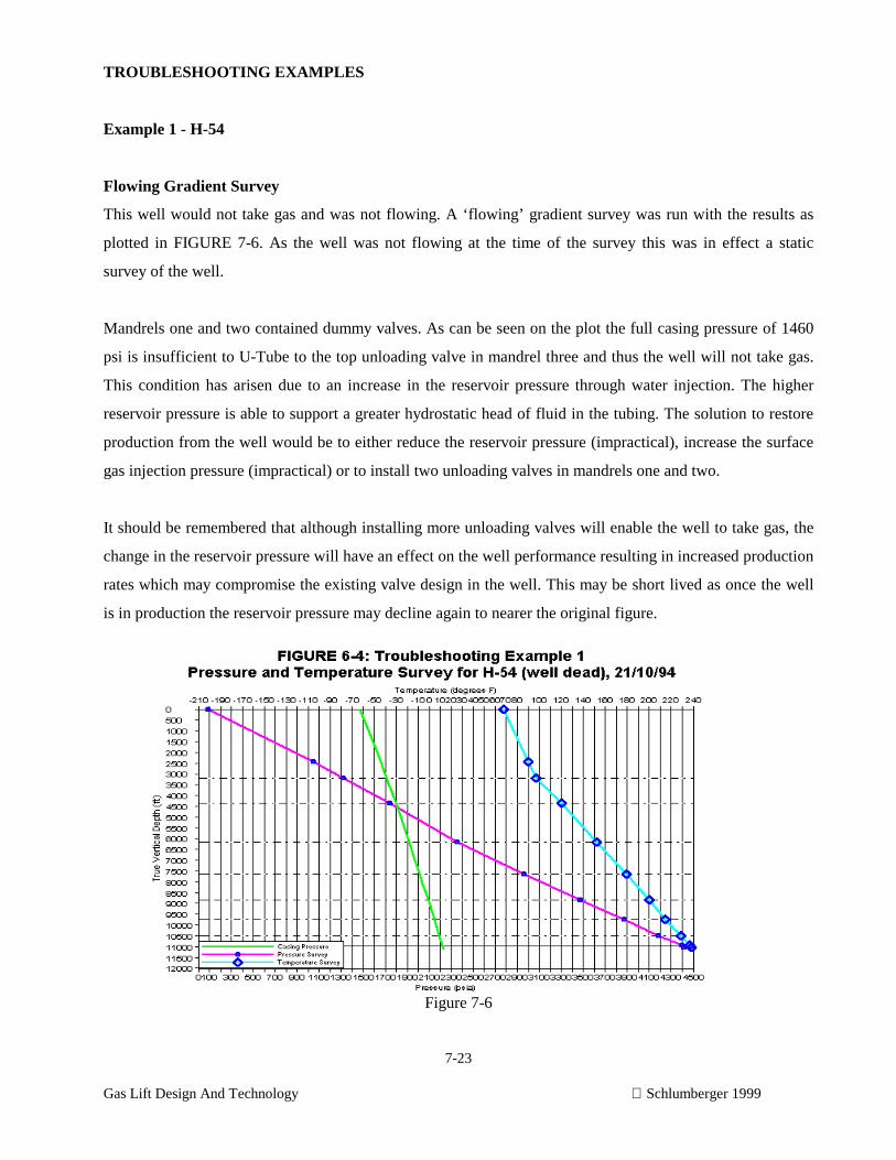
7-23
Gas Lift Design And Technology Schlumberger 1999
TROUBLESHOOTING EXAMPLES
Example 1 - H-54
Flowing Gradient Survey
This well would not take gas and was not flowing. A ‘flowing’ gradient survey was run with the results as
plotted in FIGURE 7-6. As the well was not flowing at the time of the survey this was in effect a static
survey of the well.
Mandrels one and two contained dummy valves. As can be seen on the plot the full casing pressure of 1460
psi is insufficient to U-Tube to the top unloading valve in mandrel three and thus the well will not take gas.
This condition has arisen due to an increase in the reservoir pressure through water injection. The higher
reservoir pressure is able to support a greater hydrostatic head of fluid in the tubing. The solution to restore
production from the well would be to either reduce the reservoir pressure (impractical), increase the surface
gas injection pressure (impractical) or to install two unloading valves in mandrels one and two.
It should be remembered that although installing more unloading valves will enable the well to take gas, the
change in the reservoir pressure will have an effect on the well performance resulting in increased production
rates which may compromise the existing valve design in the well. This may be short lived as once the well
is in production the reservoir pressure may decline again to nearer the original figure.
Figure 7-6
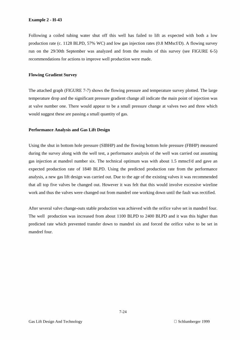
7-24
Gas Lift Design And Technology Schlumberger 1999
Example 2 - H-43
Following a coiled tubing water shut off this well has failed to lift as expected with both a low
production rate (c. 1128 BLPD, 57% WC) and low gas injection rates (0.8 MMscf/D). A flowing survey
run on the 29/30th September was analyzed and from the results of this survey (see FIGURE 6-5)
recommendations for actions to improve well production were made.
Flowing Gradient Survey
The attached graph (FIGURE 7-7) shows the flowing pressure and temperature survey plotted. The large
temperature drop and the significant pressure gradient change all indicate the main point of injection was
at valve number one. There would appear to be a small pressure change at valves two and three which
would suggest these are passing a small quantity of gas.
Performance Analysis and Gas Lift Design
Using the shut in bottom hole pressure (SIBHP) and the flowing bottom hole pressure (FBHP) measured
during the survey along with the well test, a performance analysis of the well was carried out assuming
gas injection at mandrel number six. The technical optimum was with about 1.5 mmscf/d and gave an
expected production rate of 1840 BLPD. Using the predicted production rate from the performance
analysis, a new gas lift design was carried out. Due to the age of the existing valves it was recommended
that all top five valves be changed out. However it was felt that this would involve excessive wireline
work and thus the valves were changed out from mandrel one working down until the fault was rectified.
After several valve change-outs stable production was achieved with the orifice valve set in mandrel four.
The well production was increased from about 1100 BLPD to 2400 BLPD and it was this higher than
predicted rate which prevented transfer down to mandrel six and forced the orifice valve to be set in
mandrel four.
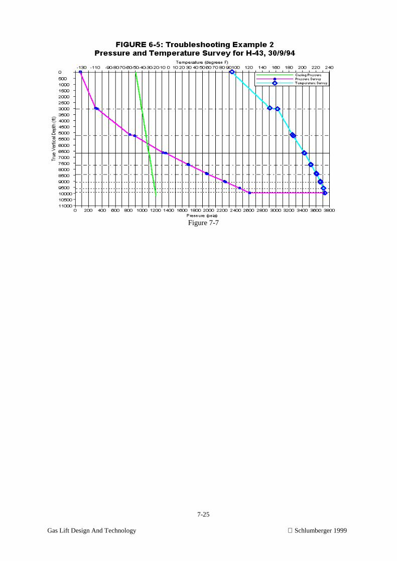
7-25
Gas Lift Design And Technology Schlumberger 1999
Figure 7-7
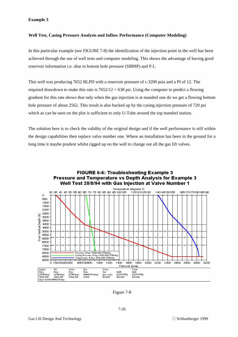
7-26
Gas Lift Design And Technology Schlumberger 1999
Example 3
Well Test, Casing Pressure Analysis and Inflow Performance (Computer Modeling)
In this particular example (see FIGURE 7-8) the identification of the injection point in the well has been
achieved through the use of well tests and computer modeling. This shows the advantage of having good
reservoir information i.e. shut in bottom hole pressure (SIBHP) and P.I..
This well was producing 7652 BLPD with a reservoir pressure of c.3200 psia and a PI of 12. The
required drawdown to make this rate is 7652/12 = 638 psi. Using the computer to predict a flowing
gradient for this rate shows that only when the gas injection is at mandrel one do we get a flowing bottom
hole pressure of about 2562. This result is also backed up by the casing injection pressure of 720 psi
which as can be seen on the plot is sufficient to only U-Tube around the top mandrel station.
The solution here is to check the validity of the original design and if the well performance is still within
the design capabilities then replace valve number one. Where an installation has been in the ground for a
long time it maybe prudent whilst rigged up on the well to change out all the gas lift valves.
Figure 7-8
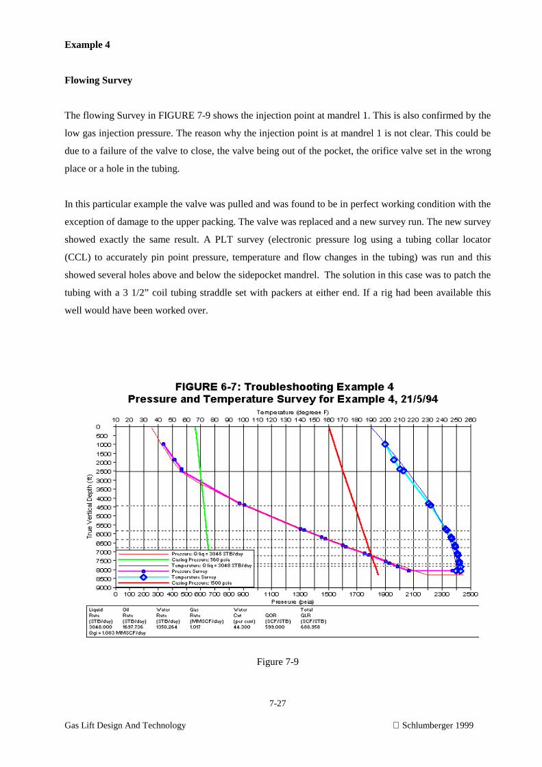
7-27
Gas Lift Design And Technology Schlumberger 1999
Example 4
Flowing Survey
The flowing Survey in FIGURE 7-9 shows the injection point at mandrel 1. This is also confirmed by the
low gas injection pressure. The reason why the injection point is at mandrel 1 is not clear. This could be
due to a failure of the valve to close, the valve being out of the pocket, the orifice valve set in the wrong
place or a hole in the tubing.
In this particular example the valve was pulled and was found to be in perfect working condition with the
exception of damage to the upper packing. The valve was replaced and a new survey run. The new survey
showed exactly the same result. A PLT survey (electronic pressure log using a tubing collar locator
(CCL) to accurately pin point pressure, temperature and flow changes in the tubing) was run and this
showed several holes above and below the sidepocket mandrel. The solution in this case was to patch the
tubing with a 3 1/2” coil tubing straddle set with packers at either end. If a rig had been available this
well would have been worked over.
Figure 7-9
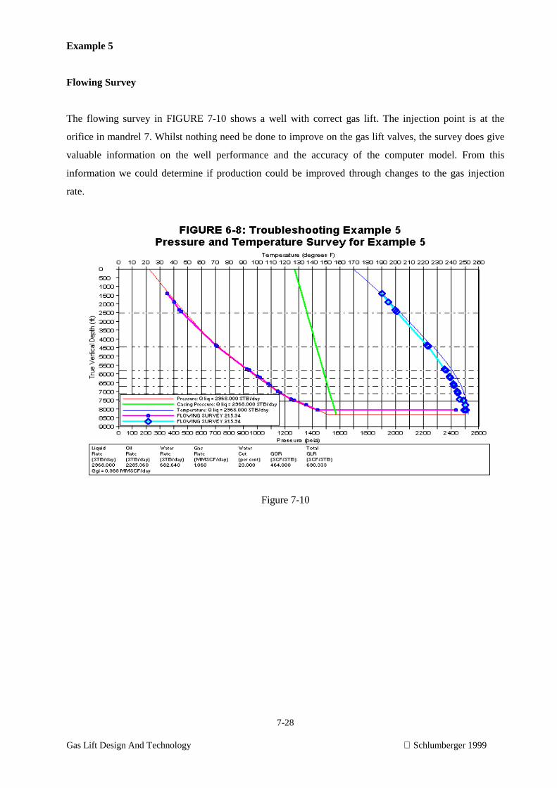
7-28
Gas Lift Design And Technology Schlumberger 1999
Example 5
Flowing Survey
The flowing survey in FIGURE 7-10 shows a well with correct gas lift. The injection point is at the
orifice in mandrel 7. Whilst nothing need be done to improve on the gas lift valves, the survey does give
valuable information on the well performance and the accuracy of the computer model. From this
information we could determine if production could be improved through changes to the gas injection
rate.
Figure 7-10
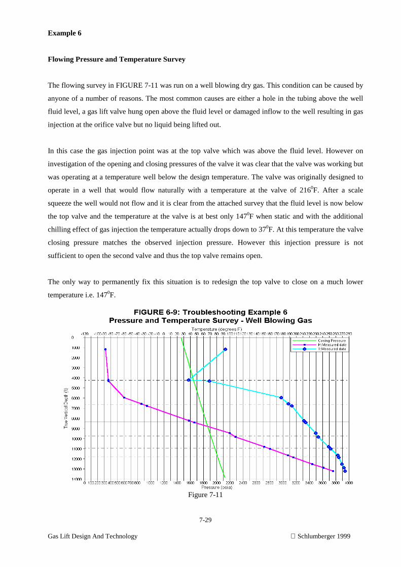
7-29
Gas Lift Design And Technology Schlumberger 1999
Example 6
Flowing Pressure and Temperature Survey
The flowing survey in FIGURE 7-11 was run on a well blowing dry gas. This condition can be caused by
anyone of a number of reasons. The most common causes are either a hole in the tubing above the well
fluid level, a gas lift valve hung open above the fluid level or damaged inflow to the well resulting in gas
injection at the orifice valve but no liquid being lifted out.
In this case the gas injection point was at the top valve which was above the fluid level. However on
investigation of the opening and closing pressures of the valve it was clear that the valve was working but
was operating at a temperature well below the design temperature. The valve was originally designed to
operate in a well that would flow naturally with a temperature at the valve of 2160F. After a scale
squeeze the well would not flow and it is clear from the attached survey that the fluid level is now below
the top valve and the temperature at the valve is at best only 1470F when static and with the additional
chilling effect of gas injection the temperature actually drops down to 370F. At this temperature the valve
closing pressure matches the observed injection pressure. However this injection pressure is not
sufficient to open the second valve and thus the top valve remains open.
The only way to permanently fix this situation is to redesign the top valve to close on a much lower
temperature i.e. 1470F.
Figure 7-11
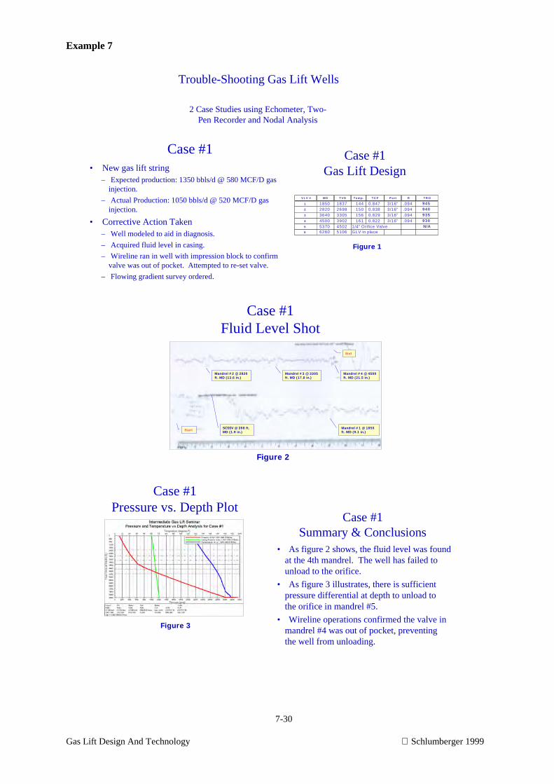
7-30
Gas Lift Design And Technology Schlumberger 1999
Example 7
Trouble-Shooting Gas Lift Wells
2 Case Studies using Echometer, Two-Pen Recorder and Nodal Analysis
Case #1• New gas lift string
– Expected production: 1350 bbls/d @ 580 MCF/D gasinjection.
– Actual Production: 1050 bbls/d @ 520 MCF/D gasinjection.
• Corrective Action Taken– Well modeled to aid in diagnosis.
– Acquired fluid level in casing.
– Wireline ran in well with impression block to confirmvalve was out of pocket. Attempted to re-set valve.
– Flowing gradient survey ordered.
Case #1Gas Lift Design
V LV # MD TV D Temp. TC F P ort R TR O
1 1850 1837 144 0.847 3/16" .094 945
2 2820 2698 150 0.838 3/16" .094 940
3 3640 3305 156 0.829 3/16" .094 935
4 4500 3902 161 0.822 3/16" .094 930
5 5370 4502 1/4" Orifice Valve N/A
6 6260 5106 GLV in place
Figure 1
Case #1Fluid Level Shot
Mandrel #1 @ 1850ft. MD (9.1 in.)Start
End
Mandrel #2 @ 2820ft. MD (13.6 in.)
Mandrel #3 @ 3305ft. MD (17.8 in.)
Mandrel #4 @ 4500ft. MD (21.5 in.)
SCSSV @ 398 ft.MD (1.9 in.)
Figure 2
Case #1Pressure vs. Depth Plot
Figure 3
Case #1Summary & Conclusions
• As figure 2 shows, the fluid level was foundat the 4th mandrel. The well has failed tounload to the orifice.
• As figure 3 illustrates, there is sufficientpressure differential at depth to unload tothe orifice in mandrel #5.
• Wireline operations confirmed the valve inmandrel #4 was out of pocket, preventingthe well from unloading.

7-31
Gas Lift Design And Technology Schlumberger 1999
Example 8
Case #2
• Well has been severely heading with tubingpressures ranging between 120 - 350 psi.Casing pressures have varied between 900 -1000 psi.
• Well believed to be multi-point injectingbetween 2 or more valves.
Case #2Gas Lift Design
VLV # MD TVD Tem p. TCF Port R TRO
1 1802 1802 105 0.912 3/16" .094 1005
2 3111 3110 121 0.884 3/16" .094 995
3 4105 4087 134 0.863 3/16" .094 980
4 4803 4747 1/4" Orifice Valve from #10 N/A
5 5418 5333 149 0.839 3/16" .094 960
6 5939 5805 156 0.829 3/16" .094 945
7 6491 6313 163 0.819 3/16" .094 930
8 7012 6794 170 0.809 3/16" .094 920
9 7563 7306 174 0.803 3/16" .094 910
10 8115 7829 N/A N/A 3/16" .094 970
Figure 4
Case #2Fluid Level Shot
Start
End
SCSSV @ 614 ft.MD (3.0 in.)
Mandrel #1 @ 1802 ft.MD (8.9 in.)
Mandrel #2 @ 3111 ft.MD (15.4 in.)
Mandrel #3 @ 4105 ft.MD (20.4 in.)
Mandrel #4 @ 4803ft. MD (23.8 in.)
Figure 5
Case #2Two-Pen Recorder Chart
Figure 6
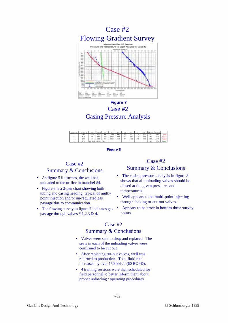
7-32
Gas Lift Design And Technology Schlumberger 1999
Case #2Flowing Gradient Survey
Figure 7
Case #2Casing Pressure Analysis
VALVE NO DEPTH TVD TRO Pd@ 60F Pt R 1-R PtR OP Tv TCF Op Force Cl Force
1 1802 1005 911 340 .0940 .9060 32 971 139 .855 912 1065 Closed
2 3110 995 901 587 .0940 .9060 55 995 147 .842 957 1071 Closed
3 4087 980 888 822 .0940 .9060 77 1020 158 .826 1001 1075 Closed
4 4747 1/4" BKO-3 Orifice Valve N/A N/A Open
Figure 8
Case #2Summary & Conclusions
• As figure 5 illustrates, the well hasunloaded to the orifice in mandrel #4.
• Figure 6 is a 2-pen chart showing bothtubing and casing heading, typical of multi-point injection and/or un-regulated gaspassage due to communication.
• The flowing survey in figure 7 indicates gaspassage through valves # 1,2,3 & 4.
Case #2Summary & Conclusions
• The casing pressure analysis in figure 8shows that all unloading valves should beclosed at the given pressures andtemperatures.
• Well appears to be multi-point injectingthrough leaking or cut-out valves.
• Appears to be error in bottom three surveypoints.
Case #2Summary & Conclusions
• Valves were sent to shop and replaced. Theseats in each of the unloading valves wereconfirmed to be cut out
• After replacing cut-out valves, well wasreturned to production. Total fluid rateincreased by over 150 bbls/d (60 BOPD).
• 4 training sessions were then scheduled forfield personnel to better inform them aboutproper unloading / operating procedures.
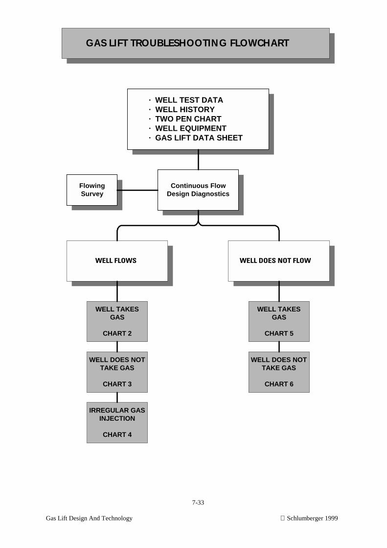
7-33
Gas Lift Design And Technology Schlumberger 1999
GAS LIFT TROUBLESHOOTING FLOWCHART
· WELL TEST DATA· WELL HISTORY· TWO PEN CHART· WELL EQUIPMENT· GAS LIFT DATA SHEET
FlowingSurvey
Continuous FlowDesign Diagnostics
WELL DOES NOT FLOW
WELL TAKESGAS
CHART 5
WELL DOES NOTTAKE GAS
CHART 6
WELL FLOWS
WELL TAKESGAS
CHART 2
WELL DOES NOTTAKE GAS
CHART 3
IRREGULAR GASINJECTION
CHART 4
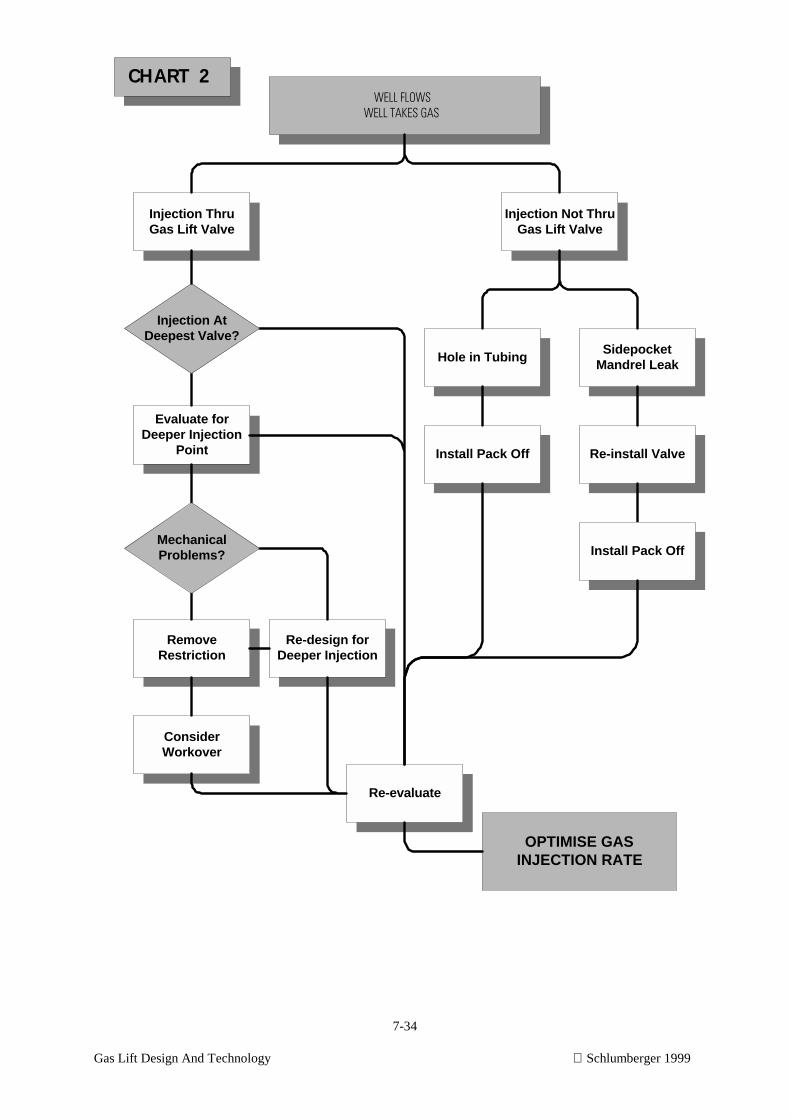
7-34
Gas Lift Design And Technology Schlumberger 1999
WELL FLOWSWELL TAKES GAS
Evaluate forDeeper Injection
Point
Injection ThruGas Lift Valve
Hole in TubingSidepocket
Mandrel Leak
Re-install ValveInstall Pack Off
Re-evaluate
Injection Not ThruGas Lift Valve
OPTIMISE GASINJECTION RATE
RemoveRestriction
ConsiderWorkover
Re-design forDeeper Injection
CHART 2
Injection AtDeepest Valve?
MechanicalProblems? Install Pack Off
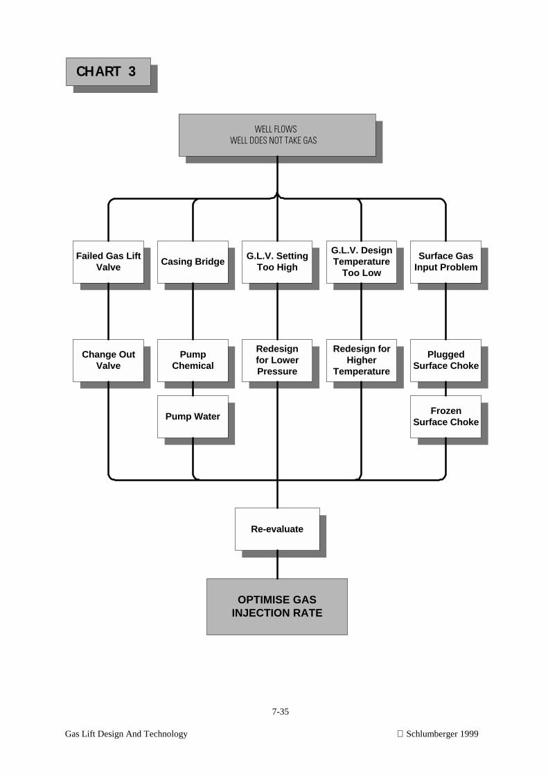
7-35
Gas Lift Design And Technology Schlumberger 1999
WELL FLOWSWELL DOES NOT TAKE GAS
Failed Gas LiftValve
Casing BridgeG.L.V. Setting
Too HighSurface Gas
Input Problem
G.L.V. DesignTemperature
Too Low
Re-evaluate
FrozenSurface Choke
Pump Water
PluggedSurface Choke
Redesign forHigher
Temperature
Redesignfor LowerPressure
PumpChemical
Change OutValve
CHART 3
OPTIMISE GASINJECTION RATE
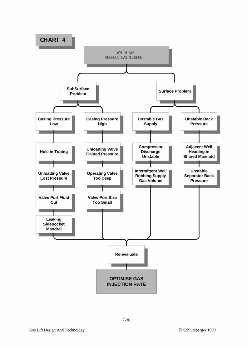
7-36
Gas Lift Design And Technology Schlumberger 1999
WELL FLOWSIRREGULAR GAS INJECTION
SubSurfaceProblem
Surface Problem
Intermittent WellRobbing Supply
Gas Volume
UnstableSeparator Back
Pressure
Re-evaluate
LeakingSidepocket
Mandrel
Valve Port FluidCut
Valve Port SizeToo Small
Operating ValveToo Deep
Unloading ValveGained Pressure
Unloading ValveLost Pressure
Hole in Tubing
Casing PressureHigh
CompressorDischargeUnstable
Adjacent WellHeading in
Shared Manifold
Unstable GasSupply
Unstable BackPressure
Casing PressureLow
CHART 4
OPTIMISE GASINJECTION RATE
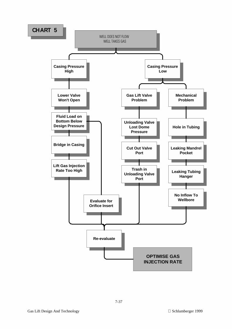
7-37
Gas Lift Design And Technology Schlumberger 1999
WELL DOES NOT FLOWWELL TAKES GAS
Casing PressureHigh
Unloading ValveLost DomePressure
Evaluate forOrifice Insert
Casing PressureLow
Hole in Tubing
Cut Out ValvePort
Trash inUnloading Valve
Port
Leaking MandrelPocket
Leaking TubingHanger
Re-evaluate
Lower ValveWon't Open
Fluid Load onBottom Below
Design Pressure
Bridge in Casing
Lift Gas InjectionRate Too High
CHART 5
OPTIMISE GASINJECTION RATE
Gas Lift ValveProblem
MechanicalProblem
No Inflow ToWellbore
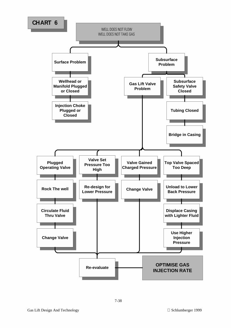
7-38
Gas Lift Design And Technology Schlumberger 1999
WELL DOES NOT FLOWWELL DOES NOT TAKE GAS
SubsurfaceProblem
SubsurfaceSafety Valve
Closed
Tubing Closed
Gas Lift ValveProblem
Bridge in Casing
Wellhead orManifold Plugged
or Closed
Injection ChokePlugged or
Closed
Surface Problem
PluggedOperating Valve
Rock The well
Circulate FluidThru Valve
Change Valve
Re-design forLower Pressure
Valve SetPressure Too
High
Valve GainedCharged Pressure
Change Valve
Top Valve SpacedToo Deep
Unload to LowerBack Pressure
Displace Casingwith Lighter Fluid
Use HigherInjectionPressure
Re-evaluate
CHART 6
OPTIMISE GASINJECTION RATE
8 - 1Gas Lift Design And Technology Schlumberger 1999
GAS LIFT DESIGN AND TECHNOLOGY
8. Reference Charts and Tables
8 - 2Gas Lift Design And Technology Schlumberger 1999
8. Reference Charts and Tables
CHAPTER OBJECTIVE: This section contains reference charts, tables and graphs
regularly used for gas lift design calculations.
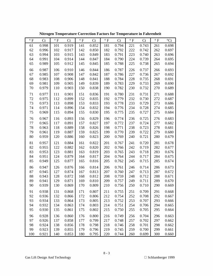
8 - 3Gas Lift Design And Technology Schlumberger 1999
Nitrogen Temperature Correction Factors for Temperature in Fahrenheit
° F Ct ° F Ct ° F Ct ° F Ct ° F Ct ° F °Ct61 0.998 101 0.919 141 0.852 181 0.794 221 0.743 261 0.69862 0.996 102 0.917 142 0.850 182 0.792 222 0.742 262 0.69763 0.994 103 0.915 143 0.849 183 0.791 223 0.740 263 0.69664 0.991 104 0.914 144 0.847 184 0.790 224 0.739 264 0.69565 0.989 105 0.912 145 0.845 185 0.788 225 0.738 265 0.694
66 0.987 106 0.910 146 0.844 186 0.787 226 0.737 266 0.69367 0.985 107 0.908 147 0.842 187 0.786 227 0.736 267 0.69268 0.983 108 0.906 148 0.841 188 0.784 228 0.735 268 0.69169 0.981 109 0.905 149 0.839 189 0.783 229 0.733 269 0.69070 0.979 110 0.903 150 0.838 190 0.782 230 0.732 270 0.689
71 0.977 111 0.901 151 0.836 191 0.780 231 0.731 271 0.68872 0.975 112 0.899 152 0.835 192 0.779 232 0.730 272 0.68773 0.973 113 0.898 153 0.833 193 0.778 233 0.729 273 0.68674 0.971 114 0.896 154 0.832 194 0.776 234 0.728 274 0.68575 0.969 115 0.894 155 0.830 195 0.775 235 0.727 275 0.684
76 0.967 116 0.893 156 0.829 196 0.774 236 0.725 276 0.68377 0.965 117 0.891 157 0.827 197 0.772 237 0.724 277 0.68278 0.963 118 0.889 158 0.826 198 0.771 238 0.723 278 0.68179 0.961 119 0.887 159 0.825 199 0.770 239 0.722 279 0.68080 0.959 120 0.886 160 0.823 200 0.769 240 0.721 280 0.679
81 0.957 121 0.884 161 0.822 201 0.767 241 0.720 281 0.67882 0.955 122 0.882 162 0.820 202 0.766 242 0.719 282 0.67783 0.953 123 0.881 163 0.819 203 0.765 243 0.718 283 0.67684 0.951 124 0.879 164 0.817 204 0.764 244 0.717 284 0.67585 0.949 125 0.877 165 0.816 205 0.762 245 0.715 285 0.674
86 0.947 126 0.876 166 0.814 206 0.761 246 0.714 286 0.67387 0.945 127 0.874 167 0.813 207 0.760 247 0.713 287 0.67288 0.943 128 0.872 168 0.812 208 0.759 248 0.712 288 0.67189 0.941 129 0.871 169 0.810 209 0.757 249 0.711 289 0.67090 0.939 130 0.869 170 0.809 210 0.756 250 0.710 290 0.669
91 0.938 131 0.868 171 0.807 211 0.755 251 0.709 291 0.66892 0.936 132 0.866 172 0.806 212 0.754 252 0.708 292 0.66793 0.934 133 0.864 173 0.805 213 0.752 253 0.707 293 0.66694 0.932 134 0.863 174 0.803 214 0.751 254 0.706 294 0.66595 0.930 135 0.861 175 0.802 215 0.750 255 0.705 295 0.664
96 0.928 136 0.860 176 0.800 216 0.749 256 0.704 296 0.66397 0.926 137 0.858 177 0.799 217 0.748 257 0.702 297 0.66298 0.924 138 0.856 178 0.798 218 0.746 258 0.701 298 0.66299 0.923 139 0.855 179 0.796 219 0.745 259 0.700 299 0.661
100 0.921 140 0.853 180 0.795 220 0.744 260 0.699 300 0.660
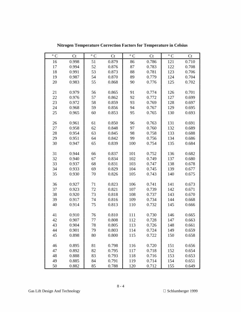
8 - 4Gas Lift Design And Technology Schlumberger 1999
Nitrogen Temperature Correction Factors for Temperature in Celsius
° C Ct ° C Ct ° C Ct ° C Ct16 0.998 51 0.879 86 0.786 121 0.71017 0.994 52 0.876 87 0.783 122 0.70818 0.991 53 0.873 88 0.781 123 0.70619 0.987 54 0.870 89 0.779 124 0.70420 0.983 55 0.868 90 0.776 125 0.702
21 0.979 56 0.865 91 0.774 126 0.70122 0.976 57 0.862 92 0.772 127 0.69923 0.972 58 0.859 93 0.769 128 0.69724 0.968 59 0.856 94 0.767 129 0.69525 0.965 60 0.853 95 0.765 130 0.693
26 0.961 61 0.850 96 0.763 131 0.69127 0.958 62 0.848 97 0.760 132 0.68928 0.954 63 0.845 98 0.758 133 0.68829 0.951 64 0.842 99 0.756 134 0.68630 0.947 65 0.839 100 0.754 135 0.684
31 0.944 66 0.837 101 0.752 136 0.68232 0.940 67 0.834 102 0.749 137 0.68033 0.937 68 0.831 103 0.747 138 0.67834 0.933 69 0.829 104 0.745 139 0.67735 0.930 70 0.826 105 0.743 140 0.675
36 0.927 71 0.823 106 0.741 141 0.67337 0.923 72 0.821 107 0.739 142 0.67138 0.920 73 0.818 108 0.737 143 0.67039 0.917 74 0.816 109 0.734 144 0.66840 0.914 75 0.813 110 0.732 145 0.666
41 0.910 76 0.810 111 0.730 146 0.66542 0.907 77 0.808 112 0.728 147 0.66343 0.904 78 0.805 113 0.726 148 0.66144 0.901 79 0.803 114 0.724 149 0.65945 0.898 80 0.800 115 0.722 150 0.658
46 0.895 81 0.798 116 0.720 151 0.65647 0.892 82 0.795 117 0.718 152 0.65448 0.888 83 0.793 118 0.716 153 0.65349 0.885 84 0.791 119 0.714 154 0.65150 0.882 85 0.788 120 0.712 155 0.649
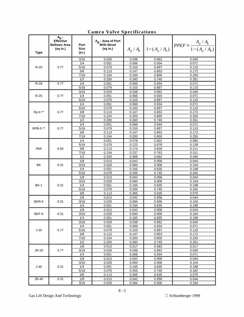
8 - 5Gas Lift Design And Technology Schlumberger 1999
Camco Valve Specifications
Type
Ab -Effective
Bellows Area(sq in.)
PortSize(in.)
Ap - Area of PortWith Bevel
(sq in.) A Ap b/ 1− ( / )A Ap b
PPEFA A
A Ap b
p b
=−
/
( / )1
3/16 0.029 0.038 0.962 0.0401/4 0.051 0.066 0.934 0.071
R-20 0.77 5/16 0.079 0.103 0.897 0.1153/8 0.113 0.147 0.853 0.1727/16 0.154 0.200 0.800 0.2501/2 0.200 0.260 0.740 0.351
R-28 0.77 1/4 0.051 0.066 0.934 0.0715/16 0.079 0.103 0.897 0.1153/16 0.029 0.038 0.962 0.040
R-25 0.77 1/4 0.051 0.066 0.934 0.0715/16 0.079 0.103 0.897 0.1151/4 0.051 0.066 0.934 0.0715/16 0.079 0.103 0.897 0.115
Rp-6 ** 0.77 3/8 0.113 0.147 0.853 0.1727/16 0.154 0.200 0.800 0.2501/2 0.200 0.260 0.740 0.3511/4 0.051 0.066 0.934 0.071
RPB-5 ** 0.77 5/16 0.079 0.103 0.897 0.1153/8 0.113 0.147 0.853 0.1727/16 0.154 0.200 0.800 0.2501/4 0.051 0.078 0.922 0.0855/16 0.079 0.122 0.878 0.139
RMI 0.65 3/8 0.113 0.174 0.826 0.2117/16 0.154 0.237 0.763 0.3111/2 0.200 0.308 0.692 0.4451/8 0.013 0.042 0.958 0.044
BK 0.31 3/16 0.029 0.094 0.906 0.1041/4 0.051 0.165 0.835 0.1985/16 0.079 0.255 0.745 0.3421/8 0.013 0.042 0.958 0.0443/16 0.029 0.094 0.906 0.104
BK-1 0.31 1/4 0.051 0.165 0.835 0.1985/16 0.079 0.255 0.745 0.3423/8 0.113 0.365 0.635 0.5751/8 0.013 0.042 0.958 0.044
BKR-5 0.31 3/16 0.029 0.094 0.906 0.1041/4 0.051 0.165 0.835 0.1981/8 0.013 0.042 0.958 0.044
BKF-6 0.31 3/16 0.029 0.094 0.906 0.1041/4 0.051 0.165 0.835 0.1983/16 0.029 0.038 0.962 0.0401/4 0.051 0.066 0.934 0.071
J-20 0.77 5/16 0.079 0.103 0.897 0.1153/8 0.113 0.147 0.853 0.1727/16 0.154 0.200 0.800 0.2501/2 0.200 0.260 0.740 0.3511/8 0.013 0.017 0.983 0.017
JR-20 0.77 3/16 0.029 0.038 0.962 0.0401/4 0.051 0.066 0.934 0.0711/8 0.013 0.042 0.958 0.0443/16 0.029 0.094 0.906 0.104
J-40 0.31 1/4 0.051 0.165 0.835 0.1985/16 0.079 0.255 0.745 0.3423/8 0.113 0.365 0.635 0.575
JR-40 0.31 1/8 0.013 0.042 0.958 0.0443/16 0.029 0.094 0.906 0.104

8 - 6Gas Lift Design And Technology Schlumberger 1999