Embed Size (px)
Citation preview
Fluid Dynamics Research 39 (2007) 98–120
Gauge principle and variational formulation for ideal fluids withreference to translation symmetry
Tsutomu Kambe
IDS, Higashi-yama 2-11-3, Meguro-ku, Tokyo 153-0043, Japan
Received 2 February 2006; received in revised form 11 June 2006; accepted 15 September 2006
Communicated by S. Kida
Abstract
Following the gauge principle in the field theory of physics, a new variational formulation is presented for flowsof an ideal fluid. In the present gauge-theoretical analysis, it is assumed that the field of fluid flow is character-ized by a translation symmetry (group) and in addition that the fluid itself is a material in motion characterizedthermodynamically by mass density and entropy (per unit mass). Local gauge transformation in the present case islocal Galilean transformation (without rotation) which is a subgroup of a generalized local Galilean transformationgroup between non-inertial frames. In complying with the requirement of local gauge invariance of Lagrangians, agauge-covariant derivative with respect to time is defined by introducing a gauge term. Galilean invariance requiresthat the covariant derivative should be the convective derivative, i.e. the so-called Lagrange derivative. Using thisgauge-covariant operator, a free-field Lagrangian and Lagrangians associated with gauge fields are defined underthe gauge symmetry. Euler’s equation of motion is derived from the action principle. Simutaneously, the equation ofcontinuity and equation of entropy conservation are derived from the variational principle. It is found that generalsolution thus obtained is equivalent to the classical Clebsch solution. If entropy of the fluid is non-uniform, the flowwill be rotational. However, if the entropy is uniform throughout the space (i.e. homentropic), then the flow fieldreduces to that of a potential flow. Discussions are given on the issue. From the gauge invariance with respect totranslational transformations, a differential conservation law of momentum is deduced as Noether’s theorem.© 2006 The Japan Society of Fluid Mechanics and Elsevier B.V. All rights reserved.
Keywords: Gauge principle; Variational principle; Ideal fluid; Translation symmetry; Covariant derivative; Clebsch solution
E-mail address: [email protected].
0169-5983/$32.00 © 2006 The Japan Society of Fluid Mechanics and Elsevier B.V. All rights reserved.doi:10.1016/j.fluiddyn.2006.09.002

T. Kambe / Fluid Dynamics Research 39 (2007) 98–120 99
1. Introduction
Fluid mechanics is a field theory in Newtonian mechanics, i.e. the field theory of mass flows subject toGalilean transformation. In the theory of gauge field, a guiding principle is that laws of physics should beexpressed in a form that is independent of any particular coordinate system. In the gauge theory of particlephysics (Weinberg, 1995/1996; Frankel, 1997;Aitchison and Hey, 1982), a free-particle Lagrangian is firstdefined for a charged particle in such a way as having an invariance under the Lorentz transformation.Next, a gauge principle is applied to the Lagrangian, requiring it to have a symmetry, i.e. the gaugeinvariance. In particular, requirement of local gauge invariance implies existence of a new gauge fieldwhich is associated with the electromagnetic field.
There are obvious differences between the fluid-flow field and the quantum field. Firstly, the field offluid flow is non-quantum, which however causes no problem since the gauge principle is independentof the quantization principle. In addition, the fluid flow is subject to the Galilean transformation insteadof the Lorentz transformation. This is not an obstacle because the former is a limiting transformation ofthe latter as the relative ratio of flow velocity to the light speed tends to an infinitesimal quantity. Thirdly,relevant gauge groups should be different. Certainly, we have to find appropriate gauge groups for fluidflows. A translation group and a rotation group would be such groups relevant to fluid flows.
Here, we seek a formulation of fluid flows which has a formal equivalence with the gauge theory inthe electromagnetism or quantum field theory. Following the scenario of the gauge principle, we defineat the outset a Galilei-invariant Lagrangian for a system of point masses which is known to have globalgauge invariance (in Mechanics by Landau and Lifshitz, 1976). We try to extend it to fluid flows. For acontinuous field such as a fluid, in addition to the global symmetry, local gauge invariance of Lagrangianis required. This is satisfied by introducing a new gauge term into time derivative term. Precise expressionsof the global and local invariance will be presented below, and explicit forms of the Lagrangian will begiven at each step of derivation.
In the present paper, we try to apply the above concept to the formulation of flows of an ideal fluid.This approach results in a unified description of flow fields and a reformulation on the basis of the gaugeprinciple, which discloses some new aspects. Usually, the convective derivative of the velocity (i.e. theLagrange derivative) is written down intuitively for the acceleration of a material particle and taken as anidentity without relying on any physical or mathematical principle. In the present formulation, the sameconvective derivative is derived as the covariant derivative in the framework of the gauge theory, which isan essential building block of the theory. Previous papers (Kambe, 2003a,b) tried to apply the concept ofthe gauge symmetry of rotational transformations to fluid flows, and found that the vorticity is the gaugefield associated with the rotational symmetry of fluid flows.
According to the traditional variational formulation referred to as Eulerian description, if the fluid ishomentropic (i.e. the fluid entropy is uniform throughout space), the action principle of an ideal fluidresults in potential flows. It is generally understood that, even in such a homentropic fluid, it shouldbe possible to have rotational flows. In fact, this is a long-standing problem (Serrin, 1959; Lin, 1963;Seliger and Whitham, 1968; Bretherton, 1970; Salmon, 1988). Lin (1963) tried to resolve this difficulty byintroducing the Lin’s constraint as a side condition, imposing invariance of Lagrangian particle coordinatesalong particle trajectories. The constraints for the variation are formulated by using Lagrange multipliers(functions of positions), which are called as potentials. In addition, the continuity equation and isentropiccondition are also taken into account by using Lagrange multipliers, where the isentropy means that eachfluid particle keeps its entropy value along its trajectory but that the fluid is not necessarily homentropic.

100 T. Kambe / Fluid Dynamics Research 39 (2007) 98–120
However, physical significance of those potentials introduced as the Lagrange multipliers is not clear.Mysteriously, the Lagrange multiplier for the continuity equation becomes the velocity potential for flowsof a homentropic fluid (without the Lin’s constraint).
The present gauge theory for fluid flows provides us a crucial key to resolve the above issues. This is themain theme of the present paper. Among the two symmetries of flows mentioned above, the present paperconcentrates on the translation symmetry, in order to focus on the theoretical framework of the gaugetheory applied to fluid flows and show its powerfulness. It is found that general solution in this formulationis equivalent to the classical Clebsch solution. The rotational symmetry will be considered elsewhere infuture, but its preliminary approach is already given in Kambe (2003a,b). Some consideration is given toscaling symmetry of the present system in Appendix C.1
Similar field-theoretic approach is taken in Jackiw (2002) by applying the ideas of particle physics tofluid mechanics in terms of Hamiltonians of canonical variables and Poisson brackets, both relativisti-cally and nonrelativistically, and extension to supersymmetry is also considered. In this monograph, thenonrelativistic part follows the traditional approach and gauge-theoretic consideration is not given to fluidmechanics. In a Galilean-invariant nonrelativistic case, symmetries of a specific model of the Chaplygingas with a particular equation of state are studied. In addition to the symmetries with respect to space–timetranslations and rotations of Galilean group, this model is shown to have a time rescaling symmetry anda space–time mixing symmetry. In addition, the Clebsch solution is featured to represent a vorticity field� = ∇ × v in terms of three scalar functions and investigate the helicity H (Chern–Simon term) for thevelocity v, where H is defined by a 3D space integral of � · v (see Appendix B for its definition).
Some backgrounds of the present theory are reviewed in the followings.
1.1. Lagrangian and symmetries
Lagrange already knew the conservation of momentum as a result of translation symmetry, which isnow understood as a global symmetry of Lagrangian. This property is generalized as the Noether theorem(Noether, 1918; Soper, 1976), and it is commonly known that all conservation laws are derived frominvariances of the Lagrangian under transformations, i.e. its symmetries. The symmetries considered inmechanics literatures are mostly global, i.e. independent of points in the space. The local symmetry whichwe are going to investigate here from the viewpoint of the gauge theory is not considered so far, at leastexplicitly in mechanics.
Schutz and Sorkin (1977) verified that any variational principle for an ideal fluid that leads to the Eulerequation of motion must be constrained. This is related to the property of fluid flows that the energy(including the mass energy) of a fluid at rest can be changed by adding entropy or adding particles (i.e.changing density) without violating the framework of the variational principle. In addition, adding auniform velocity to a uniform-flow state is again another state of uniform flow.
With regard to the gauge field, we must find an appropriate Lagrangian. In the case of the system ofcharged particles and electromagnetic field, the total Lagrangian density consists of three parts: Lp+Lpf +Lf . The part of Lagrangian associated with charged particles is Lp, while the Lf represents the Lagrangianthat depends on the electromagnetic fields only, i.e. the Lagrangian in the absence of charged particles,where Lpf is the part of interaction between the particle and fields. In order to obtain the equationsof motion of particles by the variational principle (e.g. The Classical Theory of Fields by Landau and
1 The Appendix C is added in the revised version as a response of the author to a comment of a referee.
T. Kambe / Fluid Dynamics Research 39 (2007) 98–120 101
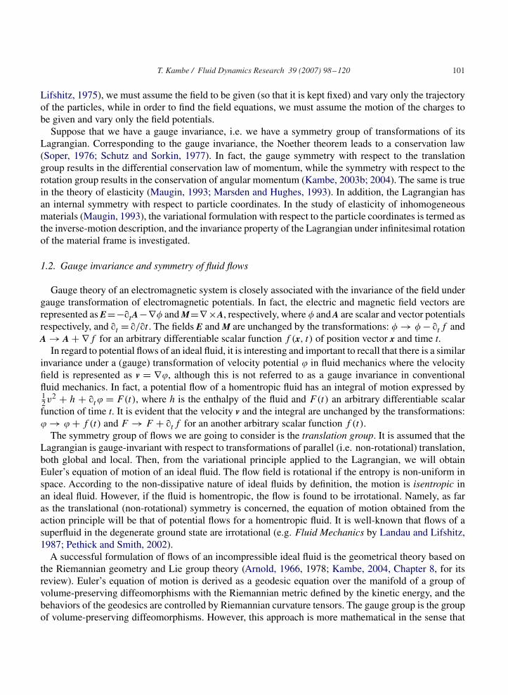
Lifshitz, 1975), we must assume the field to be given (so that it is kept fixed) and vary only the trajectoryof the particles, while in order to find the field equations, we must assume the motion of the charges tobe given and vary only the field potentials.
Suppose that we have a gauge invariance, i.e. we have a symmetry group of transformations of itsLagrangian. Corresponding to the gauge invariance, the Noether theorem leads to a conservation law(Soper, 1976; Schutz and Sorkin, 1977). In fact, the gauge symmetry with respect to the translationgroup results in the differential conservation law of momentum, while the symmetry with respect to therotation group results in the conservation of angular momentum (Kambe, 2003b; 2004). The same is truein the theory of elasticity (Maugin, 1993; Marsden and Hughes, 1993). In addition, the Lagrangian hasan internal symmetry with respect to particle coordinates. In the study of elasticity of inhomogeneousmaterials (Maugin, 1993), the variational formulation with respect to the particle coordinates is termed asthe inverse-motion description, and the invariance property of the Lagrangian under infinitesimal rotationof the material frame is investigated.
1.2. Gauge invariance and symmetry of fluid flows
Gauge theory of an electromagnetic system is closely associated with the invariance of the field undergauge transformation of electromagnetic potentials. In fact, the electric and magnetic field vectors arerepresented as E=−�tA−∇� and M=∇ ×A, respectively, where � and A are scalar and vector potentialsrespectively, and �t = �/�t . The fields E and M are unchanged by the transformations: � → � − �t f andA → A + ∇f for an arbitrary differentiable scalar function f (x, t) of position vector x and time t.
In regard to potential flows of an ideal fluid, it is interesting and important to recall that there is a similarinvariance under a (gauge) transformation of velocity potential � in fluid mechanics where the velocityfield is represented as v = ∇�, although this is not referred to as a gauge invariance in conventionalfluid mechanics. In fact, a potential flow of a homentropic fluid has an integral of motion expressed by12v2 + h + �t� = F(t), where h is the enthalpy of the fluid and F(t) an arbitrary differentiable scalarfunction of time t. It is evident that the velocity v and the integral are unchanged by the transformations:� → � + f (t) and F → F + �t f for an another arbitrary scalar function f (t).
The symmetry group of flows we are going to consider is the translation group. It is assumed that theLagrangian is gauge-invariant with respect to transformations of parallel (i.e. non-rotational) translation,both global and local. Then, from the variational principle applied to the Lagrangian, we will obtainEuler’s equation of motion of an ideal fluid. The flow field is rotational if the entropy is non-uniform inspace. According to the non-dissipative nature of ideal fluids by definition, the motion is isentropic inan ideal fluid. However, if the fluid is homentropic, the flow is found to be irrotational. Namely, as faras the translational (non-rotational) symmetry is concerned, the equation of motion obtained from theaction principle will be that of potential flows for a homentropic fluid. It is well-known that flows of asuperfluid in the degenerate ground state are irrotational (e.g. Fluid Mechanics by Landau and Lifshitz,1987; Pethick and Smith, 2002).
A successful formulation of flows of an incompressible ideal fluid is the geometrical theory based onthe Riemannian geometry and Lie group theory (Arnold, 1966, 1978; Kambe, 2004, Chapter 8, for itsreview). Euler’s equation of motion is derived as a geodesic equation over the manifold of a group ofvolume-preserving diffeomorphisms with the Riemannian metric defined by the kinetic energy, and thebehaviors of the geodesics are controlled by Riemannian curvature tensors. The gauge group is the groupof volume-preserving diffeomorphisms. However, this approach is more mathematical in the sense that
102 T. Kambe / Fluid Dynamics Research 39 (2007) 98–120
local translation and local rotation are not separated. Here we try to separate the two in order to get insightinto physics of flows.
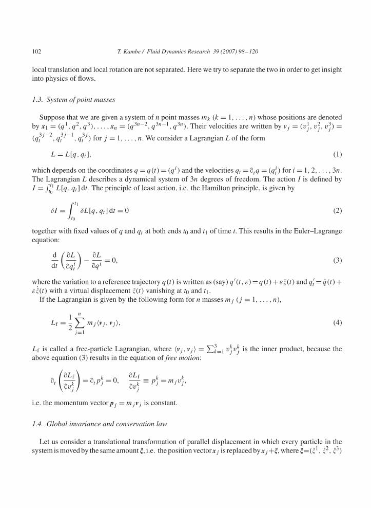
1.3. System of point masses
Suppose that we are given a system of n point masses mk (k = 1, . . . , n) whose positions are denotedby x1 = (q1, q2, q3), . . . , xn = (q3n−2, q3n−1, q3n). Their velocities are written by vj = (v1
j , v2j , v
3j ) =
(q3j−2t , q
3j−1t , q
3jt ) for j = 1, . . . , n. We consider a Lagrangian L of the form
L = L[q, qt ], (1)
which depends on the coordinates q = q(t) = (qi) and the velocities qt = �t q = (qit ) for i = 1, 2, . . . , 3n.
The Lagrangian L describes a dynamical system of 3n degrees of freedom. The action I is defined byI = ∫ t1
t0L[q, qt ] dt . The principle of least action, i.e. the Hamilton principle, is given by
�I =∫ t1
t0
�L[q, qt ] dt = 0 (2)
together with fixed values of q and qt at both ends t0 and t1 of time t. This results in the Euler–Lagrangeequation:
d
dt
(�L
�qit
)− �L
�qi= 0, (3)
where the variation to a reference trajectory q(t) is written as (say) q ′(t, ε)=q(t)+ε�(t) and q ′t = q̇(t)+
ε�̇(t) with a virtual displacement �(t) vanishing at t0 and t1.If the Lagrangian is given by the following form for n masses mj (j = 1, . . . , n),
Lf = 1
2
n∑j=1
mj 〈vj , vj 〉, (4)
Lf is called a free-particle Lagrangian, where 〈vj , vj 〉 = ∑3k=1 vk
j vkj is the inner product, because the
above equation (3) results in the equation of free motion:
�t
(�Lf
�vkj
)= �tp
kj = 0,
�Lf
�vkj
≡ pkj = mjv
kj ,
i.e. the momentum vector pj = mj vj is constant.
1.4. Global invariance and conservation law
Let us consider a translational transformation of parallel displacement in which every particle in thesystem is moved by the same amount �, i.e. the position vector xj is replaced by xj+�, where �=(�1, �2, �3)
T. Kambe / Fluid Dynamics Research 39 (2007) 98–120 103
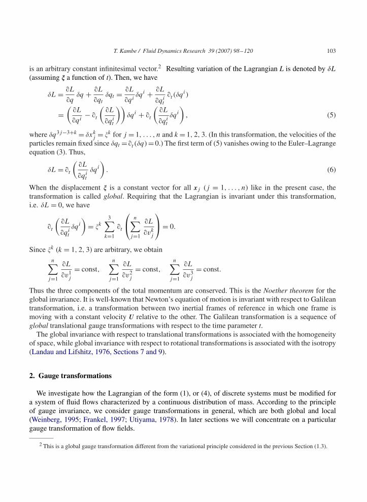
is an arbitrary constant infinitesimal vector.2 Resulting variation of the Lagrangian L is denoted by �L(assuming � a function of t). Then, we have
�L = �L
�q�q + �L
�qt
�qt = �L
�qi�qi + �L
�qit
�t (�qi)
=(
�L
�qi− �t
(�L
�qit
))�qi + �t
(�L
�qit
�qi
), (5)
where �q3j−3+k = �xkj = �k for j = 1, . . . , n and k = 1, 2, 3. (In this transformation, the velocities of the
particles remain fixed since �qt = �t (�q)=0.) The first term of (5) vanishes owing to the Euler–Lagrangeequation (3). Thus,
�L = �t
(�L
�qit
�qi
). (6)
When the displacement � is a constant vector for all xj (j = 1, . . . , n) like in the present case, thetransformation is called global. Requiring that the Lagrangian is invariant under this transformation,i.e. �L = 0, we have
�t
(�L
�qit
�qi
)= �k
3∑k=1
�t
⎛⎝ n∑
j=1
�L
�vkj
⎞⎠= 0.
Since �k (k = 1, 2, 3) are arbitrary, we obtainn∑
j=1
�L
�v1j
= const,n∑
j=1
�L
�v2j
= const,n∑
j=1
�L
�v3j
= const.
Thus the three components of the total momentum are conserved. This is the Noether theorem for theglobal invariance. It is well-known that Newton’s equation of motion is invariant with respect to Galileantransformation, i.e. a transformation between two inertial frames of reference in which one frame ismoving with a constant velocity U relative to the other. The Galilean transformation is a sequence ofglobal translational gauge transformations with respect to the time parameter t.
The global invariance with respect to translational transformations is associated with the homogeneityof space, while global invariance with respect to rotational transformations is associated with the isotropy(Landau and Lifshitz, 1976, Sections 7 and 9).
2. Gauge transformations
We investigate how the Lagrangian of the form (1), or (4), of discrete systems must be modified fora system of fluid flows characterized by a continuous distribution of mass. According to the principleof gauge invariance, we consider gauge transformations in general, which are both global and local(Weinberg, 1995; Frankel, 1997; Utiyama, 1978). In later sections we will concentrate on a particulargauge transformation of flow fields.
2 This is a global gauge transformation different from the variational principle considered in the previous Section (1.3).

104 T. Kambe / Fluid Dynamics Research 39 (2007) 98–120
Concept of local transformation is a generalization of the global transformation. When we considerlocal gauge transformation, the physical system under consideration must be modified so as to allow us toconsider a continuous field by extending the original discrete system. We replace the discrete variables qi
by continuous parameters a = (a1, a2, a3) to represent continuous distribution of particles in a sub-spaceM of three-dimensional Euclidean space E3. Spatial position x = (x1, x2, x3) of each massive particle ofthe name tag a (Lagrange parameter) is denoted by x = xa(t) ≡ X(a, t) = (Xk(a, t) ), a function of a aswell as time t. Conversely, the particle occupying the point x at a time t is denoted by a(x, t).
2.1. Continuous field and global invariance
Now, we consider a continuous distribution of mass (i.e. fluid) and its motion. The Lagrangian (1) or(4) must be modified to the following integral form:
L =∫
L(q, qt ) d3x, (7)
where L is a Lagrangian density. Suppose that an infinitesimal transformation is expressed by
q = x → q ′ = x + �x, �x = �(x, t),qt = v → q ′
t = v + �v, �v = �t (�x),
}(8)
where v = �tX(a, t), and the vector function �(x, t) is an arbitrary differentiable variation field. Resultingvariation of the Lagrangian density L(x, v) is
�L =(
�L
�x− �t
(�L
�v
))· �x + �t
(�L
�v· �x
). (9)
This does not vanish in general owing to the arbitrary function �x = �(x, t) depending on time t. In fact,assuming the Euler–Lagrange equation �L/�x − �t (�L/�v) = 0 (an extended form of (3)), we obtain
�L = �t
(�L
�v· �x
)= �t
(�L
�v
)· � + �L
�v· �t�. (10)
In the global transformation of � = const, we have �t� = 0. Then, global invariance of the Lagrangian(�L = 0) for arbitrary constant � requires
�t
∫�L
�vd3x = 0.
This states the conservation of total momentum defined by∫(�L/�v) d3x. The same result for the global
transformation (� = const and �v = �t� = 0) can be obtained directly from (7) since
�L =∫
� · �L
�xd3x = � ·
∫�t
(�L
�v
)d3x = 0, (11)
by using the above Euler–Lagrange equation. In the local transformation, however, the variation field �
depends on time t and space point x, and the variation �L = ∫�L d3x does not vanish in general.
T. Kambe / Fluid Dynamics Research 39 (2007) 98–120 105
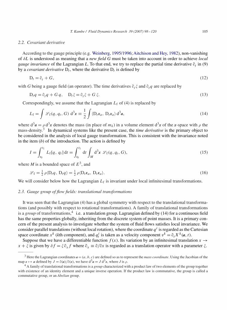
2.2. Covariant derivative
According to the gauge principle (e.g. Weinberg, 1995/1996; Aitchison and Hey, 1982), non-vanishingof �L is understood as meaning that a new field G must be taken into account in order to achieve localgauge invariance of the Lagrangian L. To that end, we try to replace the partial time derivative �t in (9)by a covariant derivative Dt , where the derivative Dt is defined by
Dt = �t + G, (12)
with G being a gauge field (an operator). The time derivatives �t� and �t q are replaced by
Dt q = �t q + Gq, Dt� = �t� + G �. (13)
Correspondingly, we assume that the Lagrangian Lf of (4) is replaced by
Lf =∫
Lf(q, qt , G) d3x ≡ 1
2
∫〈Dtxa, Dtxa〉 d3a, (14)
where d3a = � d3x denotes the mass (in place of mk) in a volume element d3x of the x-space with � themass-density.3 In dynamical systems like the present case, the time derivative is the primary object tobe considered in the analysis of local gauge transformation. This is consistent with the invariance notedin the item (b) of the introduction. The action is defined by
I =∫ t1
t0
Lf [q, qt ] dt =∫ t1
t0
dt
∫M
d3x Lf(q, qt , G), (15)
where M is a bounded space of E3, and
Lf = 12 �〈Dt q, Dt q〉 = 1
2 �〈Dtxa, Dtxa〉. (16)
We will consider below how the Lagrangian Lf is invariant under local infinitesimal transformations.
2.3. Gauge group of flow fields: translational transformations
It was seen that the Lagrangian (4) has a global symmetry with respect to the translational transforma-tions (and possibly with respect to rotational transformations). A family of translational transformationsis a group of transformations,4 i.e. a translation group. Lagrangian defined by (14) for a continuous fieldhas the same properties globally, inheriting from the discrete system of point masses. It is a primary con-cern of the present analysis to investigate whether the system of fluid flows satisfies local invariance. Weconsider parallel translations (without local rotation), where the coordinate qi is regarded as the Cartesianspace coordinate xk (kth component), and qi
t is taken as a velocity component vk = �tXk(a, t).
Suppose that we have a differentiable function f (x). Its variation by an infinitesimal translation x →x + � is given by �f = � �xf where �x ≡ �/�x is regarded as a translation operator with a parameter �.
3 Here the Lagrangian coordinates a = (a, b, c) are defined so as to represent the mass coordinate. Using the Jacobian of themap x �→ a defined by J = �(a)/�(x), we have d3a = J d3x, where J is �.
4 A family of translational transformations is a group characterized with a product law of two elements of the group togetherwith existence of an identity element and a unique inverse operation. If the product law is commutative, the group is called acommutative group, or an Abelian group.
106 T. Kambe / Fluid Dynamics Research 39 (2007) 98–120
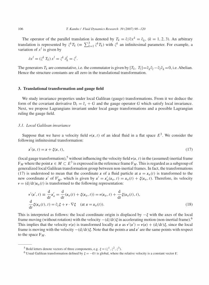
The operator of the parallel translation is denoted by Tk = �/�xk = �k , (k = 1, 2, 3). An arbitrarytranslation is represented by �kTk (≡ ∑3
k=1 �kTk) with �k an infinitesimal parameter. For example, avariation of xl is given by
�xl = (�k Tk) xl = �k �lk = �l .
The generators Tk are commutative, i.e. the commutator is given by [Tk, Tl]=�k�l −�l�k =0, i.e. Abelian.Hence the structure constants are all zero in the translational transformation.
3. Translational transformation and gauge field
We study invariance properties under local Galilean (gauge) transformations. From it we deduce theform of the covariant derivative Dt = �t + G and the gauge operator G which satisfy local invariance.Next, we propose Lagrangians invariant under local gauge transformations and a possible Lagrangianruling the gauge field.
3.1. Local Galilean invariance
Suppose that we have a velocity field v(x, t) of an ideal fluid in a flat space E3. We consider thefollowing infinitesimal transformation:
x′(x, t) = x + �(x, t), (17)
(local gauge transformation),5 without influencing the velocity field v(x, t) in the (assumed) inertial frameFM where the point x ∈ M ⊂ E3 is expressed in the reference frame FM . This is regarded as a subgroup ofgeneralized local Galilean transformation group between non-inertial frames. In fact, the transformations(17) is understood to mean that the coordinate x of a fluid particle at x = xa(t) is transformed to thenew coordinate x′ of F′
M , which is given by x′ = x′a(xa, t) = xa(t) + �(xa, t). Therefore, its velocity
v = (d/dt)xa(t) is transformed to the following representation:
v′(x′, t) ≡ d
dtx′a = d
dt(xa(t) + �(xa, t)) = v(xa, t) + d
dt�(xa(t), t),
d
dt�(xa(t), t) = �t� + v · ∇� (at x = xa(t)). (18)
This is interpreted as follows: the local coordinate origin is displaced by −� with the axes of the localframe moving (without rotation) with the velocity −(d/dt)� in accelerating motion (non-inertial frame).6
This implies that the velocity v(x) is transformed locally at x as v′(x′) = v(x) + (d/dt)�, since the localframe is moving with the velocity −(d/dt)�. Note that the points x and x′ are the same points with respectto the space FM .
5 Bold letters denote vectors of three components, e.g. � = (�1, �2, �3).6 Usual Galilean transformation defined by � = −Ut is global, where the relative velocity is a constant vector U.
T. Kambe / Fluid Dynamics Research 39 (2007) 98–120 107
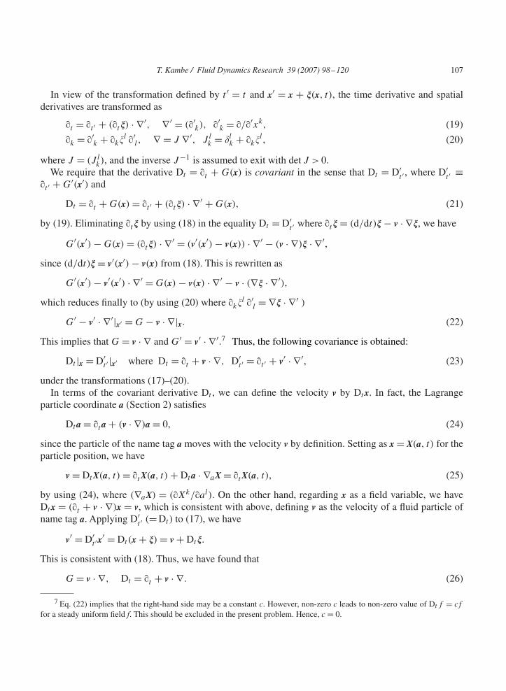
In view of the transformation defined by t ′ = t and x′ = x + �(x, t), the time derivative and spatialderivatives are transformed as
�t = �t ′ + (�t�) · ∇′, ∇′ = (�′k), �′
k = �/�′xk , (19)
�k = �′k + �k�
l �′l , ∇ = J ∇′, J l
k = �lk + �k�
l , (20)
where J = (J lk), and the inverse J−1 is assumed to exit with det J > 0.
We require that the derivative Dt = �t + G(x) is covariant in the sense that Dt = D′t ′ , where D′
t ′ ≡�t ′ + G′(x′) and
Dt = �t + G(x) = �t ′ + (�t�) · ∇′ + G(x), (21)
by (19). Eliminating �t� by using (18) in the equality Dt = D′t ′ where �t� = (d/dt)� − v · ∇�, we have
G′(x′) − G(x) = (�t�) · ∇′ = (v′(x′) − v(x)) · ∇′ − (v · ∇)� · ∇′,
since (d/dt)� = v′(x′) − v(x) from (18). This is rewritten as
G′(x′) − v′(x′) · ∇′ = G(x) − v(x) · ∇′ − v · (∇� · ∇′),
which reduces finally to (by using (20) where �k�l �′
l = ∇� · ∇′ )
G′ − v′ · ∇′|x′ = G − v · ∇|x. (22)
This implies that G = v · ∇ and G′ = v′ · ∇′.7 Thus, the following covariance is obtained:
Dt |x = D′t ′ |x′ where Dt = �t + v · ∇, D′
t ′ = �t ′ + v′ · ∇′, (23)
under the transformations (17)–(20).In terms of the covariant derivative Dt , we can define the velocity v by Dtx. In fact, the Lagrange
particle coordinate a (Section 2) satisfies
Dta = �ta + (v · ∇)a = 0, (24)
since the particle of the name tag a moves with the velocity v by definition. Setting as x = X(a, t) for theparticle position, we have
v = DtX(a, t) = �tX(a, t) + Dta · ∇aX = �tX(a, t), (25)
by using (24), where (∇aX) = (�Xk/�al). On the other hand, regarding x as a field variable, we haveDtx = (�t + v · ∇)x = v, which is consistent with above, defining v as the velocity of a fluid particle ofname tag a. Applying D′
t ′ (= Dt ) to (17), we have
v′ = D′t ′x
′ = Dt (x + �) = v + Dt�.
This is consistent with (18). Thus, we have found that
G = v · ∇, Dt = �t + v · ∇. (26)
7 Eq. (22) implies that the right-hand side may be a constant c. However, non-zero c leads to non-zero value of Dt f = cf
for a steady uniform field f. This should be excluded in the present problem. Hence, c = 0.
108 T. Kambe / Fluid Dynamics Research 39 (2007) 98–120
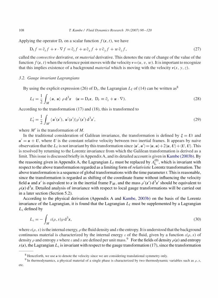
Applying the operator Dt on a scalar function f (x, t), we have
Dt f = �t f + v · ∇f = �t f + u �xf + v �yf + w �zf , (27)
called the convective derivative, or material derivative. This denotes the rate of change of the value of thefunction f (x, t) when the reference point moves with the velocity v=(u, v, w). It is important to recognizethat this implies existence of a background material which is moving with the velocity v(x, y, z).
3.2. Gauge invariant Lagrangians
By using the explicit expression (26) of Dt , the Lagrangian Lf of (14) can be written as8
Lf = 1
2
∫M
〈 u, u〉 � d3x (u = Dtx, Dt ≡ �t + u · ∇). (28)
According to the transformation (17) and (18), this is transformed to
L′f = 1
2
∫M ′
〈 u′(x′), u′(x′)〉�′(x′) d3x′, (29)
where M ′ is the transformation of M.In the traditional consideration of Galilean invariance, the transformation is defined by � = Ut and
u′ = u + U, where U is the constant relative velocity between two inertial frames. It appears by naiveobservation that the Lf is not invariant by this transformation since 〈u′, u′〉=〈u, u〉+2〈u, U〉+〈U, U〉. Thisis resolved by returning to the Lorentz invariance from which the Galilean transformation is derived as alimit. This issue is discussed briefly inAppendixA, and its detailed account is given in Kambe (2003b). Bythe reasoning given in Appendix A, the Lagrangian Lf must be replaced by �(0)
L , which is invariant withrespect to the above transformation regarded as a limiting form of relativistic Lorentz transformation. Theabove transformation is a sequence of global transformations with the time parameter t. This is reasonable,since the transformation is regarded as shifting of the coordinate frame without influencing the velocityfield u and x′ is equivalent to x in the inertial frame FM , and the mass �′(x′) d3x′ should be equivalent to�(x) d3x. Detailed analysis of invariance with respect to local gauge transformations will be carried outin a later section (Section 5.2).
According to the physical derivation (Appendix A and Kambe, 2003b) on the basis of the Lorentzinvariance of the Lagrangian, it is found that the Lagrangian Lf must be supplemented by a LagrangianL� defined by
L� = −∫
M
�(�, s)� d3x, (30)
where �(�, s) is the internal energy, � the fluid density and s the entropy. It is understood that the backgroundcontinuous material is characterized by the internal energy � of the fluid, given by a function �(�, s) ofdensity � and entropy s where � and s are defined per unit mass.9 For the fields of density �(x) and entropys(x), the Lagrangian L� is invariant with respect to the gauge transformation (17), since the transformation
8 Henceforth, we use u to denote the velocity since we are considering translational symmetry only.9 In thermodynamics, a physical material of a single phase is characterized by two thermodynamic variables such as �, s,
etc.
T. Kambe / Fluid Dynamics Research 39 (2007) 98–120 109
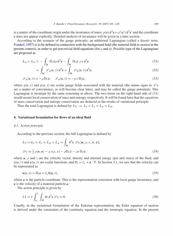
is a matter of the coordinate origin under the invariance of mass: �(x) d3x =�′(x′) d3x′ and the coordinatex does not appear explicitly. Detailed analysis of invariance will be given in a later section.
According to the scenario of the gauge principle, an additional Lagrangian (called a kinetic term,Frankel, 1997) is to be defined in connection with the background field (the material field in motion in thepresent context), in order to get non-trivial field equations (for � and s). Possible type of the Lagrangiansare proposed as
L� + L = −∫
M
Dt�� d3x −∫
M
Dt � s d3x (31)
=∫
M
L�(x, t) d3x +∫
M
L(x, t) d3x, (32)
L�(x, t) = −� Dt�, L(x, t) = −� s Dt, (33)
where �(x, t) and (x, t) are scalar gauge fields associated with the material (the minus signs in L’sare a matter of convenience, as will become clear later), and may be called the gauge potentials. ThisLagrangian is invariant by the same reasoning as above. The two terms on the right-hand side of (31)would assure local conservation of mass and entropy, respectively. It will be found later that the equationsof mass conservation and entropy conservation are deduced as the results of variational principle.
Thus the total Lagrangian is defined by LT := Lf + L� + L� + L.
4. Variational formulation for flows of an ideal fluid
4.1. Action principle
According to the previous section, the full Lagrangian is defined by
LT = Lf + L� + L� + L =∫
M
d3x LT [u, �, s, �, ],
LT ≡ 12 �〈u, u〉 − � �(�, s) − �Dt� − �s Dt, (34)
where u, � and � are the velocity vector, density and internal energy (per unit mass) of the fluid, and�(x, t) and (x, t) are scalar functions, and Dt = �t + u · ∇. In Section 3.1, we saw that the velocity canbe represented as
u(x, t) = Dtx = �tX(a, t), (35)
where a is the particle coordinate. This is the representation consistent with local gauge invariance, andu is the velocity of a material particle a.
The action principle is given by
� I = �
∫ t1
t0
∫M
dt d3xLT = 0. (36)
Usually, in the variational formulation of the Eulerian representation, the Euler equation of motionis derived under the constraints of the continuity equation and the isentropic equation. In the present
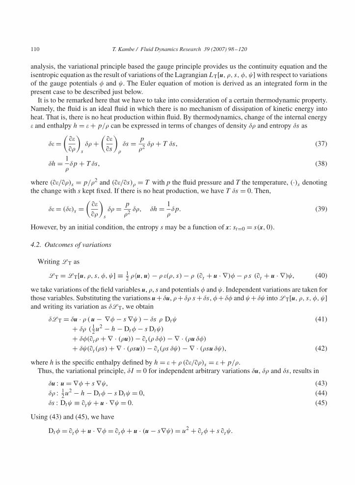
110 T. Kambe / Fluid Dynamics Research 39 (2007) 98–120
analysis, the variational principle based the gauge principle provides us the continuity equation and theisentropic equation as the result of variations of the Lagrangian LT[u, �, s, �, ] with respect to variationsof the gauge potentials � and . The Euler equation of motion is derived as an integrated form in thepresent case to be described just below.
It is to be remarked here that we have to take into consideration of a certain thermodynamic property.Namely, the fluid is an ideal fluid in which there is no mechanism of dissipation of kinetic energy intoheat. That is, there is no heat production within fluid. By thermodynamics, change of the internal energy� and enthalpy h = � + p/� can be expressed in terms of changes of density �� and entropy �s as
�� =(
��
��
)s
�� +(
��
�s
)�
�s = p
�2 �� + T �s, (37)
�h = 1
��p + T �s, (38)
where (��/��)s = p/�2 and (��/�s)� = T with p the fluid pressure and T the temperature, (·)s denotingthe change with s kept fixed. If there is no heat production, we have T �s = 0. Then,
�� = (��)s =(
��
��
)s
�� = p
�2 ��, �h = 1
��p. (39)
However, by an initial condition, the entropy s may be a function of x: st=0 = s(x, 0).
4.2. Outcomes of variations
Writing LT as
LT = LT[u, �, s, �, ] ≡ 12 �〈u, u〉 − � �(�, s) − � (�t + u · ∇)� − � s (�t + u · ∇), (40)
we take variations of the field variables u, �, s and potentials � and . Independent variations are taken forthose variables. Substituting the variations u+�u, �+�� s +�s, �+�� and +� into LT[u, �, s, �, ]and writing its variation as �LT, we obtain
�LT = �u · � ( u − ∇� − s ∇ ) − �s � Dt (41)+ �� (1
2u2 − h − Dt� − s Dt)
+ ��(�t� + ∇ · (�u)) − �t (� ��) − ∇ · (�u ��)
+ �(�t (�s) + ∇ · (�su)) − �t (�s �) − ∇ · (�su �), (42)
where h is the specific enthalpy defined by h = � + � (��/��)s = � + p/�.Thus, the variational principle, �I = 0 for independent arbitrary variations �u, �� and �s, results in
�u : u = ∇� + s ∇, (43)�� : 1
2u2 − h − Dt� − s Dt = 0, (44)�s : Dt ≡ �t + u · ∇ = 0. (45)
Using (43) and (45), we have
Dt� = �t� + u · ∇� = �t� + u · (u − s∇) = u2 + �t� + s �t.
T. Kambe / Fluid Dynamics Research 39 (2007) 98–120 111
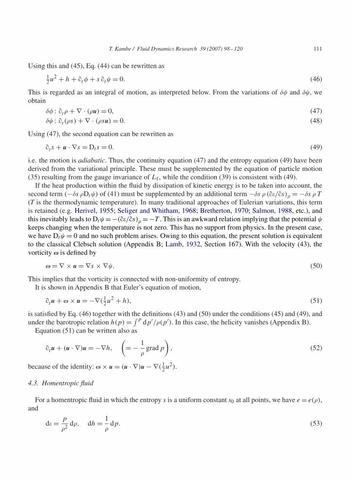
Using this and (45), Eq. (44) can be rewritten as
12u2 + h + �t� + s �t = 0. (46)
This is regarded as an integral of motion, as interpreted below. From the variations of �� and �, weobtain
�� : �t� + ∇ · (�u) = 0, (47)� : �t (�s) + ∇ · (�su) = 0. (48)
Using (47), the second equation can be rewritten as
�t s + u · ∇s = Dt s = 0. (49)
i.e. the motion is adiabatic. Thus, the continuity equation (47) and the entropy equation (49) have beenderived from the variational principle. These must be supplemented by the equation of particle motion(35) resulting from the gauge invariance of Lf , while the condition (39) is consistent with (49).
If the heat production within the fluid by dissipation of kinetic energy is to be taken into account, thesecond term (−�s �Dt) of (41) must be supplemented by an additional term −�s � (��/�s)� = −�s � T
(T is the thermodynamic temperature). In many traditional approaches of Eulerian variations, this termis retained (e.g. Herivel, 1955; Seliger and Whitham, 1968; Bretherton, 1970; Salmon, 1988, etc.), andthis inevitably leads to Dt=−(��/�s)� =−T . This is an awkward relation implying that the potential keeps changing when the temperature is not zero. This has no support from physics. In the present case,we have Dt = 0 and no such problem arises. Owing to this equation, the present solution is equivalentto the classical Clebsch solution (Appendix B; Lamb, 1932, Section 167). With the velocity (43), thevorticity � is defined by
� = ∇ × u = ∇s × ∇. (50)
This implies that the vorticity is connected with non-uniformity of entropy.It is shown in Appendix B that Euler’s equation of motion,
�tu + � × u = −∇(12u2 + h), (51)
is satisfied by Eq. (46) together with the definitions (43) and (50) under the conditions (45) and (49), andunder the barotropic relation h(p) = ∫ p dp′/�(p′). In this case, the helicity vanishes (Appendix B).
Equation (51) can be written also as
�tu + (u · ∇)u = −∇h,
(= − 1
�grad p
), (52)
because of the identity: � × u = (u · ∇)u − ∇(12u2).
4.3. Homentropic fluid
For a homentropic fluid in which the entropy s is a uniform constant s0 at all points, we have e = e(�),and
d� = p
�2 d�, dh = 1
�dp. (53)
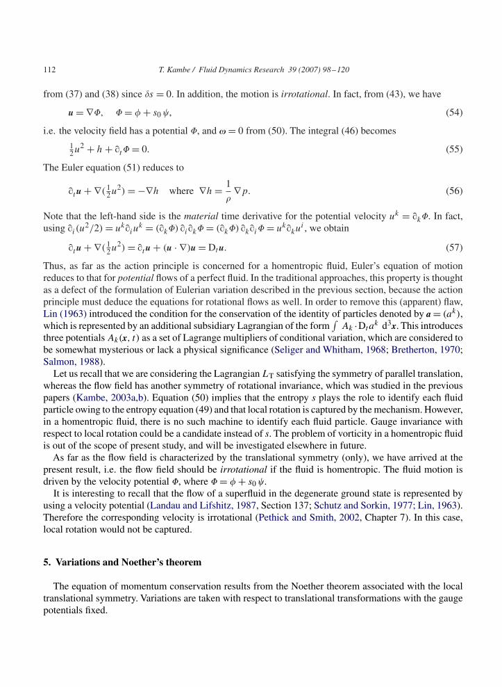
112 T. Kambe / Fluid Dynamics Research 39 (2007) 98–120
from (37) and (38) since �s = 0. In addition, the motion is irrotational. In fact, from (43), we have
u = ∇, = � + s0 , (54)
i.e. the velocity field has a potential , and � = 0 from (50). The integral (46) becomes
12u2 + h + �t = 0. (55)
The Euler equation (51) reduces to
�tu + ∇(12u2) = −∇h where ∇h = 1
�∇p. (56)
Note that the left-hand side is the material time derivative for the potential velocity uk = �k. In fact,using �i(u
2/2) = uk�iuk = (�k) �i�k = (�k) �k�i = uk�ku
i , we obtain
�tu + ∇(12u2) = �tu + (u · ∇)u = Dtu. (57)
Thus, as far as the action principle is concerned for a homentropic fluid, Euler’s equation of motionreduces to that for potential flows of a perfect fluid. In the traditional approaches, this property is thoughtas a defect of the formulation of Eulerian variation described in the previous section, because the actionprinciple must deduce the equations for rotational flows as well. In order to remove this (apparent) flaw,Lin (1963) introduced the condition for the conservation of the identity of particles denoted by a = (ak),which is represented by an additional subsidiary Lagrangian of the form
∫Ak ·Dt a
k d3x. This introducesthree potentials Ak(x, t) as a set of Lagrange multipliers of conditional variation, which are considered tobe somewhat mysterious or lack a physical significance (Seliger and Whitham, 1968; Bretherton, 1970;Salmon, 1988).
Let us recall that we are considering the Lagrangian LT satisfying the symmetry of parallel translation,whereas the flow field has another symmetry of rotational invariance, which was studied in the previouspapers (Kambe, 2003a,b). Equation (50) implies that the entropy s plays the role to identify each fluidparticle owing to the entropy equation (49) and that local rotation is captured by the mechanism. However,in a homentropic fluid, there is no such machine to identify each fluid particle. Gauge invariance withrespect to local rotation could be a candidate instead of s. The problem of vorticity in a homentropic fluidis out of the scope of present study, and will be investigated elsewhere in future.
As far as the flow field is characterized by the translational symmetry (only), we have arrived at thepresent result, i.e. the flow field should be irrotational if the fluid is homentropic. The fluid motion isdriven by the velocity potential , where = � + s0 .
It is interesting to recall that the flow of a superfluid in the degenerate ground state is represented byusing a velocity potential (Landau and Lifshitz, 1987, Section 137; Schutz and Sorkin, 1977; Lin, 1963).Therefore the corresponding velocity is irrotational (Pethick and Smith, 2002, Chapter 7). In this case,local rotation would not be captured.
5. Variations and Noether’s theorem
The equation of momentum conservation results from the Noether theorem associated with the localtranslational symmetry. Variations are taken with respect to translational transformations with the gaugepotentials fixed.
T. Kambe / Fluid Dynamics Research 39 (2007) 98–120 113
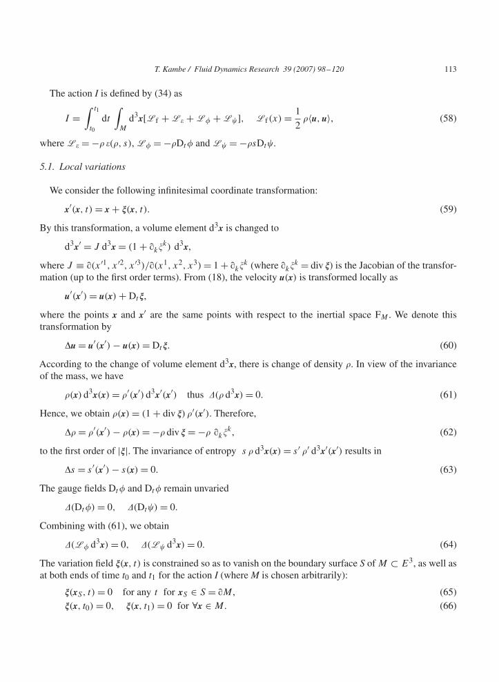
The action I is defined by (34) as
I =∫ t1
t0
dt
∫M
d3x[Lf + L� + L� + L], Lf(x) = 1
2�〈u, u〉, (58)
where L� = −� �(�, s), L� = −�Dt� and L = −�sDt.
5.1. Local variations
We consider the following infinitesimal coordinate transformation:
x′(x, t) = x + �(x, t). (59)
By this transformation, a volume element d3x is changed to
d3x′ = J d3x = (1 + �k�k) d3x,
where J ≡ �(x′1, x′2, x′3)/�(x1, x2, x3) = 1 + �k�k (where �k�
k = div �) is the Jacobian of the transfor-mation (up to the first order terms). From (18), the velocity u(x) is transformed locally as
u′(x′) = u(x) + Dt�,
where the points x and x′ are the same points with respect to the inertial space FM . We denote thistransformation by
�u = u′(x′) − u(x) = Dt�. (60)
According to the change of volume element d3x, there is change of density �. In view of the invarianceof the mass, we have
�(x) d3x(x) = �′(x′) d3x′(x′) thus �(� d3x) = 0. (61)
Hence, we obtain �(x) = (1 + div �) �′(x′). Therefore,
�� = �′(x′) − �(x) = −� div � = −� �k�k , (62)
to the first order of |�|. The invariance of entropy s � d3x(x) = s′ �′ d3x′(x′) results in
�s = s′(x′) − s(x) = 0. (63)
The gauge fields Dt� and Dt� remain unvaried
�(Dt�) = 0, �(Dt) = 0.
Combining with (61), we obtain
�(L� d3x) = 0, �(L d3x) = 0. (64)
The variation field �(x, t) is constrained so as to vanish on the boundary surface S of M ⊂ E3, as well asat both ends of time t0 and t1 for the action I (where M is chosen arbitrarily):
�(xS, t) = 0 for any t for xS ∈ S = �M , (65)�(x, t0) = 0, �(x, t1) = 0 for ∀x ∈ M . (66)
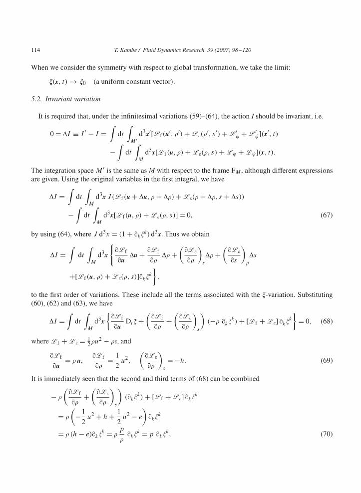
114 T. Kambe / Fluid Dynamics Research 39 (2007) 98–120
When we consider the symmetry with respect to global transformation, we take the limit:
�(x, t) → �0 (a uniform constant vector).
5.2. Invariant variation
It is required that, under the infinitesimal variations (59)–(64), the action I should be invariant, i.e.
0 = �I ≡ I ′ − I =∫
dt
∫M ′
d3x′[Lf(u′, �′) + L�(�′, s′) + L′
� + L′](x′, t)
−∫
dt
∫M
d3x[Lf(u, �) + L�(�, s) + L� + L](x, t).
The integration space M ′ is the same as M with respect to the frame FM , although different expressionsare given. Using the original variables in the first integral, we have
�I =∫
dt
∫M
d3x J (Lf(u + �u, � + ��) + L�(� + ��, s + �s))
−∫
dt
∫M
d3x[Lf(u, �) + L�(�, s)] = 0, (67)
by using (64), where J d3x = (1 + �k�k) d3x. Thus we obtain
�I =∫
dt
∫M
d3x
{�Lf
�u�u + �Lf
���� +
(�L�
��
)s
�� +(
�L�
�s
)��s
+[Lf(u, �) + L�(�, s)]�k�k
},
to the first order of variations. These include all the terms associated with the �-variation. Substituting(60), (62) and (63), we have
�I =∫
dt
∫M
d3x
{�Lf
�uDt� +
(�Lf
��+(
�L�
��
)s
)(−� �k�
k) + [Lf + L�] �k�k
}= 0, (68)
where Lf + L� = 12�u2 − ��, and
�Lf
�u= � u,
�Lf
��= 1
2u2,
(�L�
��
)s
= −h. (69)
It is immediately seen that the second and third terms of (68) can be combined
− �
(�Lf
��+(
�L�
��
)s
)(�k�
k) + [Lf + L�] �k�k
= �
(−1
2u2 + h + 1
2u2 − e
)�k�
k
= � (h − e)�k�k = �
p
��k�
k = p �k�k , (70)
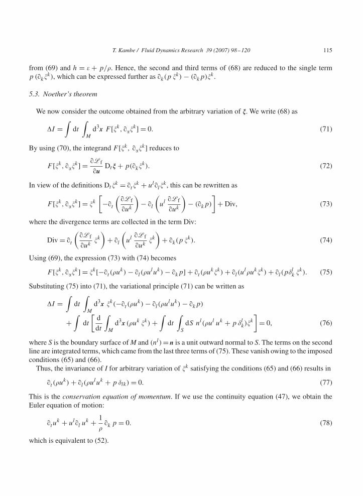
T. Kambe / Fluid Dynamics Research 39 (2007) 98–120 115
from (69) and h = � + p/�. Hence, the second and third terms of (68) are reduced to the single termp (�k�
k), which can be expressed further as �k(p �k) − (�kp)�k .
5.3. Noether’s theorem
We now consider the outcome obtained from the arbitrary variation of �. We write (68) as
�I =∫
dt
∫M
d3x F [�k, ���k] = 0. (71)
By using (70), the integrand F [�k, ���k] reduces to
F [�k, ���k] = �Lf
�uDt� + p(�k�
k). (72)
In view of the definitions Dt�k = �t�
k + ul�l�k , this can be rewritten as
F [�k, ���k] = �k
[−�t
(�Lf
�uk
)− �l
(ul �Lf
�uk
)− (�kp)
]+ Div, (73)
where the divergence terms are collected in the term Div:
Div = �t
(�Lf
�uk�k
)+ �l
(ul �Lf
�uk�k
)+ �k(p �k). (74)
Using (69), the expression (73) with (74) becomes
F [�k, ���k] = �k[−�t (�uk) − �l(�uluk) − �kp] + �t (�uk�k) + �l(u
l�uk�k) + �l(p�lk �k). (75)
Substituting (75) into (71), the variational principle (71) can be written as
�I =∫
dt
∫M
d3x �k(−�t (�uk) − �l(�uluk) − �kp)
+∫
dt
[d
dt
∫M
d3x (�uk �k) +∫
dt
∫S
dS nl(�ul uk + p �lk)�
k
]= 0, (76)
where S is the boundary surface of M and (nl)= n is a unit outward normal to S. The terms on the secondline are integrated terms, which came from the last three terms of (75). These vanish owing to the imposedconditions (65) and (66).
Thus, the invariance of I for arbitrary variation of �k satisfying the conditions (65) and (66) results in
�t (�uk) + �l(�uluk + p �lk) = 0. (77)
This is the conservation equation of momentum. If we use the continuity equation (47), we obtain theEuler equation of motion:
�tuk + ul�l u
k + 1
��k p = 0. (78)
which is equivalent to (52).
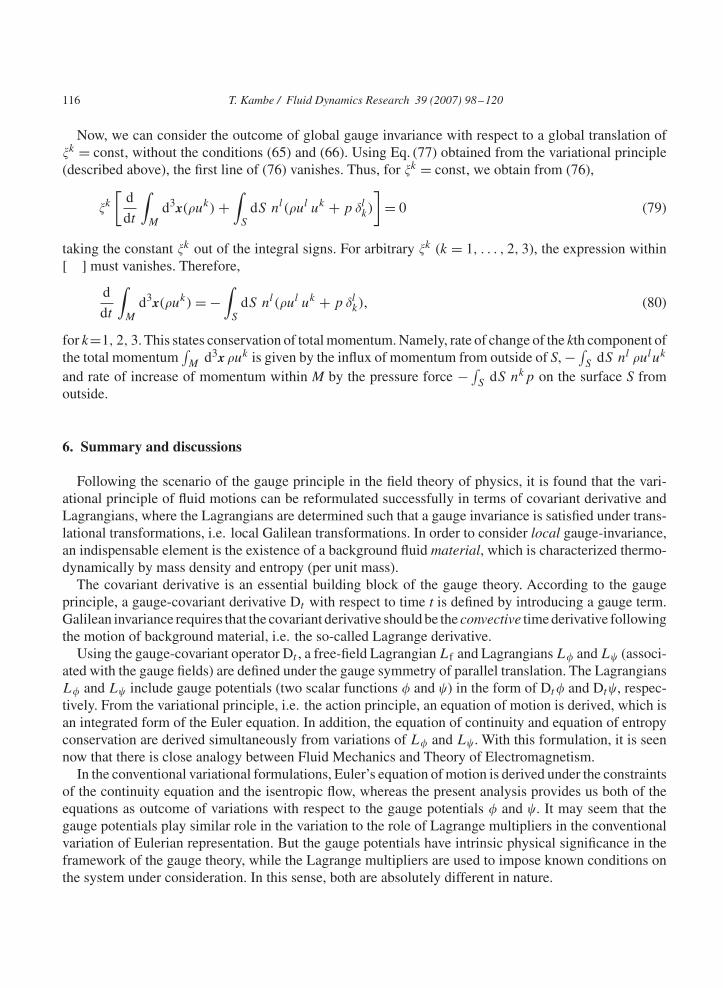
116 T. Kambe / Fluid Dynamics Research 39 (2007) 98–120
Now, we can consider the outcome of global gauge invariance with respect to a global translation of�k = const, without the conditions (65) and (66). Using Eq. (77) obtained from the variational principle(described above), the first line of (76) vanishes. Thus, for �k = const, we obtain from (76),
�k
[d
dt
∫M
d3x(�uk) +∫
S
dS nl(�ul uk + p �lk)
]= 0 (79)
taking the constant �k out of the integral signs. For arbitrary �k (k = 1, . . . , 2, 3), the expression within[ ] must vanishes. Therefore,
d
dt
∫M
d3x(�uk) = −∫
S
dS nl(�ul uk + p �lk), (80)
for k=1, 2, 3. This states conservation of total momentum. Namely, rate of change of the kth component ofthe total momentum
∫M
d3x �uk is given by the influx of momentum from outside of S, − ∫S
dS nl �uluk
and rate of increase of momentum within M by the pressure force − ∫S
dS nkp on the surface S fromoutside.
6. Summary and discussions
Following the scenario of the gauge principle in the field theory of physics, it is found that the vari-ational principle of fluid motions can be reformulated successfully in terms of covariant derivative andLagrangians, where the Lagrangians are determined such that a gauge invariance is satisfied under trans-lational transformations, i.e. local Galilean transformations. In order to consider local gauge-invariance,an indispensable element is the existence of a background fluid material, which is characterized thermo-dynamically by mass density and entropy (per unit mass).
The covariant derivative is an essential building block of the gauge theory. According to the gaugeprinciple, a gauge-covariant derivative Dt with respect to time t is defined by introducing a gauge term.Galilean invariance requires that the covariant derivative should be the convective time derivative followingthe motion of background material, i.e. the so-called Lagrange derivative.
Using the gauge-covariant operator Dt , a free-field Lagrangian Lf and Lagrangians L� and L (associ-ated with the gauge fields) are defined under the gauge symmetry of parallel translation. The LagrangiansL� and L include gauge potentials (two scalar functions � and ) in the form of Dt� and Dt, respec-tively. From the variational principle, i.e. the action principle, an equation of motion is derived, which isan integrated form of the Euler equation. In addition, the equation of continuity and equation of entropyconservation are derived simultaneously from variations of L� and L. With this formulation, it is seennow that there is close analogy between Fluid Mechanics and Theory of Electromagnetism.
In the conventional variational formulations, Euler’s equation of motion is derived under the constraintsof the continuity equation and the isentropic flow, whereas the present analysis provides us both of theequations as outcome of variations with respect to the gauge potentials � and . It may seem that thegauge potentials play similar role in the variation to the role of Lagrange multipliers in the conventionalvariation of Eulerian representation. But the gauge potentials have intrinsic physical significance in theframework of the gauge theory, while the Lagrange multipliers are used to impose known conditions onthe system under consideration. In this sense, both are absolutely different in nature.
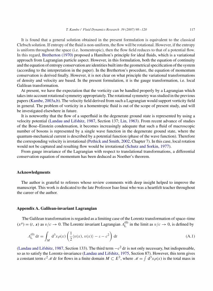
T. Kambe / Fluid Dynamics Research 39 (2007) 98–120 117
It is found that a general solution obtained in the present formulation is equivalent to the classicalClebsch solution. If entropy of the fluid is non-uniform, the flow will be rotational. However, if the entropyis uniform throughout the space (i.e. homentropic), then the flow field reduces to that of a potential flow.In this regard, Bretherton (1970) proposed a Hamilton’s principle for ideal fluids, which is a variationalapproach from Lagrangian particle aspect. However, in this formulation, both the equation of continuityand the equation of entropy conservation are identities built into the geometrical specification of the system(according to the interpretation in the paper). In the Bretherton’s procedure, the equation of momentumconservation is derived finally. However, it is not clear on what principle the variational transformationsof density and velocity are based. In the present formulation, it is the gauge transformation, i.e. localGalilean transformation.
At present, we have the expectation that the vorticity can be handled properly by a Lagrangian whichtakes into account rotational symmetry appropriately. The rotational symmetry was studied in the previouspapers (Kambe, 2003a,b). The velocity field derived from such a Lagrangian would support vorticity fieldin general. The problem of vorticity in a homentropic fluid is out of the scope of present study, and willbe investigated elsewhere in future.
It is noteworthy that the flow of a superfluid in the degenerate ground state is represented by using avelocity potential (Landau and Lifshitz, 1987, Section 137; Lin, 1963). From recent advance of studiesof the Bose–Einstein condensation, it becomes increasingly adequate that such a fluid of macroscopicnumber of bosons is represented by a single wave function in the degenerate ground state, where thequantum-mechanical current is described by a potential function (phase of the wave function). Thereforethe corresponding velocity is irrotational (Pethick and Smith, 2002, Chapter 7). In this case, local rotationwould not be captured and resulting flow would be irrotational (Schutz and Sorkin, 1977).
From gauge invariance of the Lagrangian with respect to translational transformations, a differentialconservation equation of momentum has been deduced as Noether’s theorem.
Acknowledgments
The author is grateful to referees whose review comments with deep insight helped to improve themanuscript. This work is dedicated to the late Professor Isao Imai who was a heartfelt teacher throughoutthe career of the author.
Appendix A. Galilean-invariant Lagrangian
The Galilean transformation is regarded as a limiting case of the Lorentz transformation of space–time(x ) = (t, x) as v/c → 0. The Lorentz invariant Lagrangian �(0)
L in the limit as v/c → 0, is defined by
�(0)L dt =
∫M
d3x�(x)
(1
2〈v(x), v(x)〉 − � − c2
)dt (A.1)
(Landau and Lifshitz, 1987, Section 133). The third term −c2 dt is not only necessary, but indispensable,so as to satisfy the Lorentz-invariance (Landau and Lifshitz, 1975, Section 87). However, this term givesa constant term c2M dt for flows in a finite domain M ⊂ E3, where M = ∫
d3x�(x) is the total mass in

118 T. Kambe / Fluid Dynamics Research 39 (2007) 98–120
the domain M. In carrying out variations, the total mass M is fixed to a constant. Only when we need toconsider the Galilean invariance, we must use this Lagrangian �(0)
L , rather than the LF of (28).
Appendix B. Clebsch solution
According to Lamb (1932, Section 167), the Euler equation of motion,
�tv + � × v = −∇(
1
2v2 +
∫ x dp
�
), (B.1)
with p = p(�), can be solved in general by
v = ∇� + � ∇, (B.2)1
2v2 + h + �t� + � �t = 0, h =
∫dp
�, (B.3)
Dt� = 0, Dt = 0, Dt = �t + v · ∇, (B.4)
where �, , are scalar functions of x. The continuity equation provides an equation for the potential �.This solution represents the vorticity � = ∇ × v in the form,
� = ∇� × ∇. (B.5)
In fact, using (B.2) and (B.5), we have
�tv + � × v = ∇(�t� + � �t) + (Dt�)∇ − (Dt)∇�,
where the last two terms vanish due to (B.4). Thus, Eq. (B.1) implies (B.3) where integration constant canbe absorbed in the function �. The vortex lines are the intersections of the families of surfaces � = constand = const. These surfaces are moving with the fluid by (B.4). If the scalar product � · v is integratedover a volume V including a number of closed vortex filaments, the helicity H [V ] vanishes
H [V ] ≡∫
V
� · v d3x =∫
V
(∇� × ∇) · ∇� d3x =∫
V
∇ · [� �] d3x = 0
(Bretherton, 1970). For a general velocity field, the helicity H is a measure of knottedness of the vortexlines and does not vanish in general.
Appendix C. Scale invariance
Suppose that we have an action functional defined by
I =∫ ∫
dt d3xL(t, x), L = 1
2� u2 − � �(�) − � Dt�, (C.1)
where the velocity u is irrotational and represented by u = ∇� and � is the internal energy per unit mass.This is the action for flows of a fluid of uniform entropy with the velocity potential � and in this case � isa function of density � only (Section 4.3). Consider the following scaling transformation:
t → t ′ = e2� t, x → x′ = e�x, (C.2)
T. Kambe / Fluid Dynamics Research 39 (2007) 98–120 119
where � is a parameter of transformation. Under this, the fields transform as
� → �′ = e−3��, � → �′ = e−2��, h → h′ = e−2�h,
u → u′ = e−�u, � → �′ = �, Dt → D′t = e−2�Dt ,
where D=�t +u ·∇. It is immediately checked that the action is invariant by this scaling transformation:L = L′.
Using the relation that Dt� = �t� + u · ∇� = �t� + u2, the Lagrangian density L can be written as
L = −��t� − H, H ≡ 12�u2 + V (�), V = � �, (C.3)
where H is a Hamiltonian density. Integrating by part, this is rewritten as
L = � �t − H,
where �t = �t� and the term �t (� �) is omitted in view of the time integral of (C.1). This implies that� and � are mutually-conjugate canonical variables with � a generalized coordinate and � its associatedmomentum.
Writing (C.2) as x′ = X (x, �) with t = x0 and x = (x1, x2, x3), the Noether theorem is given by theconservation equation � J
= 0, where the conserved current J ( = 0, 1, 2, 3) is defined by
J = L�X
��
∣∣∣∣�=0
+ �L
�(� �)
[��′
��− ���
�X�
��
]�=0
(Soper, 1976, Section 9.1). Using the explicit form of X , L and H given above, we obtain �X /��= x
and ��′/�� = −3� at � = 0. The current is given by Jk = xk L (k = 1, 2, 3) and
J0 = 2t L + � (−3� − 2t�t − xk�k�) = −2t H + xk �uk − �k(xk ��),
where �L/�(� �) = �. Thus, the conserved quantity is given by
J 0 = −2t H +∫
xk �uk d3x,
H =∫ (
1
2� u2 + V (�)
)d3x, V (�) = � �(�) =
∫ �
h(�′) d�′, (C.4)
where H is the total energy which is also conserved. In fact, we have
�tH =∫ (
1
2u2 + h
)�t� d3x +
∫�uk �tu
k = 0.
This can be verified by using the continuity equation (47) and the equation of motion (52). Similarly, wehave the invariance of J 0,
�t J0 = −2H +
∫xk �t (�uk) d3x = 0,
for a monoatomic gas of thermodynamic property V = c��/(�−1) and p = c�� with �= 53 (c: a constant),
by using the momentum conservation equation (77). See Jackiw (2002) for the conserved quantities ofthe Chaplygin gas.
120 T. Kambe / Fluid Dynamics Research 39 (2007) 98–120
Another example of scale invariance is given by Newtonian gravitational interaction in which theinteraction potential is described by
V = G
∫�(x) �(x′)|x − x′| d3x′, G: gravitation constant.
The scale invariance is obtained if the transformation law is as follows:
x → x′ = e�x, t → t ′ = e(3/2)� t ,
u → u′ = e−(1/2)�u, � → �′ = e−3��.
This implies Kepler’s third law.
References
Aitchison, I.J.R., Hey, A.J.G., 1982. Gauge Theories in Particle Physics. Adams Hilger, Bristol.Arnold, V.I., 1966/1978. Sur la géométrie différentielle des groupes de Lie de dimension infinie et ses applications a
l’hydrodynamique des fluides parfaits.Ann. Inst. Fourier (Grenoble) 16, 319–361; Mathematical Methods of Classical Physics,Appendix 2. Springer, Berlin.
Bretherton, F.P., 1970. A note on Hamilton’s principle for perfect fluids. J. Fluid Mech. 44, 19–31.Frankel, T., 1997. The Geometry of Physics an Introduction. Cambridge University Press, Cambridge.Herivel, J.W., 1955. The derivation of the equations of motion of an ideal fluid by Hamilton’s principle. Proc. Cambridge Phil.
Soc. 51, 344–349.Jackiw, R., 2002. Lectures on Fluid Dynamics: A Particle Theorist’s View of Supersymmetric, Non-Abelian, Noncommutative
Fluid Mechanics and D-Branes. Springer, Berlin.Kambe, T., 2003a. Gauge principle for flows of a perfect fluid. Fluid Dyn. Res. 32, 193–199.Kambe, T., 2003b. Gauge principle and variational formulation for flows of an ideal fluid. Acta Mech. Sin. 19, 437–452.Kambe, T., 2004. Geometrical Theory of Dynamical Systems and Fluid Flows. World Scientific Publishing, Singapore.Lamb, H., 1932. Hydrodynamics. Cambridge University Press, Cambridge.Landau, L.D., Lifshitz, E.M., 1975. The Classical Theory of Fields. fourth ed. Pergamon Press, New York.Landau, L.D., Lifshitz, E.M., 1976. Mechanics. third ed. Pergamon Press, New York.Landau, L.D., Lifshitz, E.M., 1987. Fluid Mechanics. second ed. Pergamon Press, New York.Lin, C.C., 1963. Hydrodynamics of helium II, in Liquid Helium. Proc. Int. Sch. Phys. Enrico Fermi XXI. Academic Press, NY,
pp. 93–146.Marsden, J.E., Hughes, T.J.R., 1993. Mathematical Foundations of Elasticity. Dover, New York.Maugin, G.A., 1993. Material Inhomogeneities in Elasticity. Chapman & Hall, London.Noether, E., 1918. Invariante Variationsproblem. Klg-Ges. Wiss. Nach. Göttingen, Math. Physik Kl, 2, 235.Pethick, C.J., Smith, H., 2002. Bose–Einstein condensation. Cambridge University Press, Cambridge.Salmon, R., 1988. Hamiltonian fluid mechanics. Ann. Rev. Fluid Mech. 20, 225–256.Schutz, B.F., Sorkin, R., 1977. Variational aspects of relativistic field theories, with application to perfect fluids. Ann. Phys. 107,
1–43.Seliger, R.L., Whitham, G.B., 1968. Variational principle in continuum mechanics. Proc. Roy. Soc. A 305, 1–25.Serrin, J., 1959. Mathematical principles of classical fluid mechanics. In: Flügge, Truesdell, C. (Eds.), Encyclopedia of Physics.
Springer, Berlin, pp. 125–263.Soper, D.E., 1976. Classical Field Theory. Wiley, New York.Utiyama, R., 1978. Theory of General Relativity [in Japanese], Syokabo (Tokyo, Japan); Utiyama R 1956. Invariant theoretical
interpretation of interaction. Phys. Rev. A 101, 1597–1607.Weinberg, S., 1995/1996. The Quantum Theory of Fields. vols. I and II. Cambridge University Press, Cambridge.