Gaussian Based Hue Descriptors - Computing Science ...funt/Mirzaei+Funt_GaussianHue_PAMI2015.pdfpseudo-color atlas as the representation of hue. Such Gaussian-like reflectances have

0162-8828 (c) 2015 IEEE. Personal use is permitted, but republication/redistribution requires IEEE permission. Seehttp://www.ieee.org/publications_standards/publications/rights/index.html for more information.

This article has been accepted for publication in a future issue of this journal, but has not been fully edited. Content may change prior to final publication. Citation information: DOI10.1109/TPAMI.2015.2420560, IEEE Transactions on Pattern Analysis and Machine Intelligence

1

Abstract— A robust and accurate hue descriptor that is useful

in modeling human color perception and for computer vision applications is explored. The hue descriptor is based on the peak wavelength of a Gaussian-like function (called a wraparound Gaussian) and is shown to correlate as well as CIECAM02 hue to the hue designators of papers from the Munsell and Natural Color System color atlases and to the hue names found in Moroney’s Color Thesaurus. The new hue descriptor is also shown to be significantly more stable under a variety of illuminants than CIECAM02. The use of wraparound Gaussians as a hue model is similar in spirit to the use of subtractive Gaussians proposed by Mizokami et al., but overcomes many of their limitations.

Index Terms—Color, hue, Gaussian reflectance, wraparound Gaussian, color atlas.

I. INTRODUCTION UE is an important component of color appearance. We explore a representation of hue

for object colors in which, for a given color stimulus arising from the light reflected by an object, its hue is represented in terms of the peak wavelength of a Gaussian-like reflectance function metameric to that stimulus. Conventionally, hue is represented in terms of the angular component of the polar representation of a color in an opponent color space such as CIELAB in which two of the axes are roughly orthogonal to lightness [1]. Although these color spaces may work well for a fixed illuminant, they can lead to unstable results when the illuminant is changed. The source of this instability is that CIELAB and related spaces account for the illumination via von Kries scaling, but von Kries scaling can be subject to very large errors [2]. This is a serious problem even when the scaling is applied in a ‘sharpened’ [3] basis as in CIECAM02 [4].

To overcome this problem, we explore [5][6]

This work was supported in part by the Natural Sciences and Engineering The authors are with the School of Computing Science, Simon Fraser

University, Burnaby, B.C. Canada V5A 1S6. (e-mails: [email protected] and [email protected]).

basing hue on the peak wavelength of a metameric Gaussian-like reflectance from Logvinenko’s pseudo-color atlas as the representation of hue. Such Gaussian-like reflectances have been used previously as a tool for predicting how a color signal (i.e., cone response triple) changes with a change in illumination [7]. Similar, but somewhat different, Gaussian-based representations of hue have been proposed previously by Mizokami et al. [8][9] and further explored by O’Neil et al. [10] and shown to explain the class of hue shifts known as the Abney effect. As well, Mizokami et al. have shown that Gaussian-like functions can be used to provide reasonable 3-dimensional models of reflectance spectra.

The tests reported below demonstrate that the proposed hue descriptor correlates well with the hue designators for the 1600 glossy Munsell papers and the Natural Color System samples. It also correlates well with the hue names used in Moroney’s Color Thesaurus. In addition, to correlating well with the hue categories in these datasets, we find that it is considerably more consistent under different illuminants than CIECAM02 hue. Given these features, we show that it is also useful for automatic hue classification in digital images.

II. BACKGROUND The Gaussian-like representation for hue used here

has its roots in Logvinenko’s illumination-invariant object-color atlas [11]. In contrast to CIELAB/CIECAM02, his object-color atlas provides a coordinate system that does not change with a change in illuminant. The atlas is defined in terms of a special set of optimal spectral reflectance functions, no pair of which becomes metameric under any strictly positive illuminant (p λ >0; 380 ≤ λ ≤ 780). For any sensor set and strictly positive illuminant spectral power distribution, any color stimulus (i.e., cone response triple) maps to a

Gaussian-Based Hue Descriptors Hamidreza Mirzaei and Brian Funt

H



2

unique element of the object-color atlas—in particular, to the element metameric to it under the given illuminant. The atlas’s rectangular reflectance functions are defined as a mixture of flat grey (constant reflectance of 0.5) and a rectangular optimal reflectance component taking only values 0 or 1, with at most 2 transitions between 0 and 1.

Given λ1 and λ2 as transition wavelengths, it is also possible to express the optimal reflectance functions by their central wavelength 𝜆 =(λ1 + λ2)/2 and spectral bandwidth 𝛿 = 𝜆2−𝜆1 (see [11] Eqs. (13) and (14) for complete definition). We will refer to the triple αδλ as ADL coordinates.

The 3-parameters of the atlas, α (chromatic purity), δ (spectral bandwidth) and λ (central wavelength) were shown [11] to be rough perceptual correlates of apparent purity, whiteness/blackness, and hue, respectively. When the illumination changes, the mapping of object colors to the rectangular atlas coordinates—and hence of the perceptual correlates too—is subject to a phenomenon referred to as color stimulus shift. Although the object-color atlas itself is illumination invariant, this does not mean that an object’s coordinate specification within the atlas will not change with the illumination. This is simply a consequence of the fact that two objects that are metameric under one illuminant may no longer be metameric under a different illuminant. In the case of the rectangular object color atlas, this means that the coordinates of the object may change as the object becomes metameric to a different one of the atlas’s rectangular functions.

The effect of color stimulus shift is exacerbated by the fact that, by their very nature, the rectangular functions include two very sudden jumps, one up and the other down. In a subsequent paper, Logvinenko [12] suggests a “wraparound” Gaussian parameterization of the rectangular color atlas. Since Gaussians are smooth, and hence more like natural reflectances, they may mitigate the effects of color stimulus shift.

Logvinenko’s wraparound Gaussian representation follows from, but also differs from, earlier such representations such as proposed by Weinberg [13] and Mizokami et al. [8]. The parameterization of the rectangular color atlas

involves reflectances defined in terms of 3-parameter wraparound Gaussian functions

defined as follows: If :

For (1)

For (2)

On the other hand when :

For (3)

For (4)

where are the ends of the visible spectrum, and . For ,

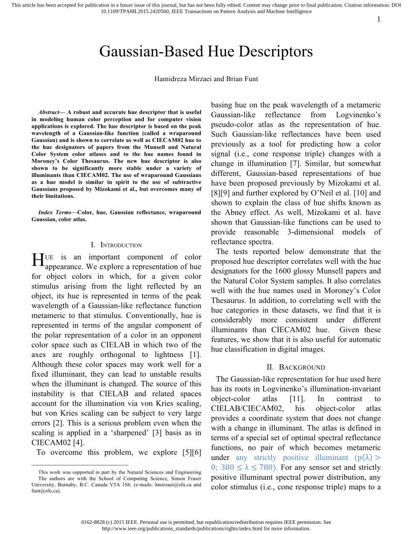
and positive , we have a Gaussian-like reflectance function (i.e., it is everywhere between 0 and 1). Although the function definitions are piecewise and a bit complex, intuitively they simply describe a Gaussian-like function centered at µ on the hue circle. We will refer to the triple kσµ as KSM coordinates, where σ stands for standard deviation, µ for peak wavelength, and k for scaling. Fig. 1 shows an example of a wraparound Gaussian metamer and a rectangular metamer for the spectral reflectance of Munsell paper 5 YR 5/6 under D65. In this, and all other cases below, the calculations are based on the 2-degree standard observer color matching functions [14]. The color matching functions are only available at finite number of discrete wavelengths (5nm spacing) so when calculating metamers values at intermediate wavelengths are interpolated.

Fig. 1. The spectral reflectance of Munsell 5 YR 5/6 (dashed black) illuminated

by D65 and its metameric rectangular (dashed blue), subtractive Gaussian (dashed green), and wraparound Gaussian (solid red) spectra. Results are for the 𝐶𝐼𝐸 1931 𝑥𝑦𝑧 2-degree standard observer.

Logvinenko parameterizes the rectangular object

( ; , , )g kλ σ µ

( )/2max minµ λ µ≤ +

/2minλ λ µ≤ ≤ +Λ 2( ; , , ) exp[ ( ) ]g k kλ θ µ θ λ µ= − −

/2 maxµ λ λ+Λ ≤ ≤ 2( ; , , ) exp[ ( ) ]g k kλ θ µ θ λ µ= − − −Λ

( )/2max minµ λ µ≥ +

/2minλ λ µ≤ ≤ −Λ 2( ; , , ) exp[ ( ) ]g k kλ θ µ θ λ µ= − − +Λ

/2 maxµ λ λ−Λ ≤ ≤ 2( ; , , ) exp[ ( ) ]g k kλ θ µ θ λ µ= − −

max minandλ λ

max minλ λΛ= − 21/θ σ= 0 1k≤ ≤

min maxλ µ λ≤ ≤ θ

CIE 1931 x y z



3

color atlas using the wraparound Gaussians as follows. “If for any rectangular metamer 𝑟 𝜆;𝛼, 𝛿, 𝜆 and a positive light 𝑝 𝜆 the equations (i=1,2,3)

𝑟 𝜆;𝛼, 𝛿, 𝜆 𝑝 𝜆 𝑠! 𝜆 𝑑𝜆

!!"#

!!"#

= 𝑔! 𝜆; 𝑘!, 𝜃!, µμ! 𝑝 𝜆 𝑠!(𝜆)𝑑𝜆

!!"!

!!"#

(5)

have a unique solution with respect to the triplet (𝑘!,𝜃!, µμ!), we will say that we have the Gaussian representation of the rectangle color atlas.” [12]. In other words, if the conditions are met then for illuminant p(λ) there is a one-to-one mapping between the kσµ and αδλ coordinate systems. Logvinenko does not provide a proof as to when these conditions will be met; however, numerical testing has not yet yielded a counterexample except along the achromatic, black-white axis, where a singularity is to be expected. Note that for the case of sampled data such as the CIE color matching functions a proof will not be possible without additional assumptions about the form of the color matching functions.

III. COMPARISON TO OTHER GAUSSIAN-LIKE MODELS

Note that Logvinenko’s wraparound Gaussians are neither the same as the “inverse Gaussians” defined by Weinberg [13] and later used by MacLeod et al. [15] nor the same as the “subtractive Gaussians” defined by Mizokami et al. [8]. In the inverse Gaussian representation, illuminant and reflectance spectra are characterized by three parameters: the spectral centroid, spectral curvature, and scaling factor. The inverse Gaussian spectrum P(λ) is defined as:

𝑃 𝜆 = γ. 𝑒!!(!!!)! (6) where γ is the scaling factor, C is the curvature and T is the centroid. Note that depending on the sign of the quadratic term these functions are either Gaussians or the reciprocals of Gaussians. In the subtractive Gaussian representation [6] the spectra

are specified in terms of the amplitude (𝛼), peak wavelength (𝜙), and standard deviation (σ) of the function:

𝑆 𝜆 = α𝑒!!.!(!!!! )! for α ≥ 0

1+ α𝑒!!.!(!!!! )! for α < 0

(7)

We will refer to these two cases as Gaussians of

type G+ and type G-, respectively. In a previous study [7] we compared (see Fig. 2 of

[7] page 1682) the gamuts of chromaticities in the CIE 1931 XYZ tri-stimulus space for subtractive Gaussians, inverse Gaussians, and wraparound Gaussians under illuminant CIE D65 and found that neither subtractive Gaussians nor inverse Gaussians can cover the entire chromaticity gamut when the functions are restricted to being reflectance functions (i.e., all values in [0,1]). On the other hand, wraparound Gaussians do cover the entire chromaticity gamut. Given an XYZ, the parameters of the subtractive and wraparound Gaussians can be found via a two-parameter optimization [7] that is independent of the scaling parameter; however, in the case of inverse Gaussians such a decomposition is not possible, so a much more difficult, three-parameter optimization is required. Given that inverse Gaussians are more difficult to compute and do not cover the chromaticity gamut, we do not consider them further here.

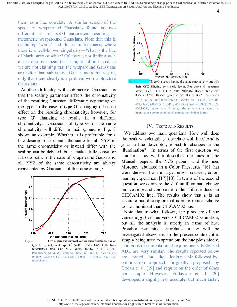
The work of Mizokami et al. [8][9] and O’Neil et al. [10] has shown that Gaussian spectra may provide a good model of hue in the case of lights. However, there are some difficulties that arise in applying Gaussians of the subtractive type as a descriptor of hue for objects. In particular, the G+ and G- chromaticity gamuts overlap (see Fig. 2(a) of [7]) or Fig. 8. (a) page 17 of [9]) quite significantly. For the wraparound Gaussian, however, there is no such overlap (see Fig. 2(c) of [7]). The overlap for the subtractive Gaussians implies that for a given XYZ we might find metameric Gaussians of both type G+ and G-. Searching for just such a case, we easily found the example shown in Fig. 2. The fact that there are two metameric (up to 4-digit precision) subtractive Gaussians differing significantly in their peak wavelengths (380nm versus 621nm) poses a serious impediment to using



4

them as a hue correlate. A similar search of the space of wraparound Gaussians found no two different sets of KSM parameters resulting in metameric wraparound Gaussians. Note that this is excluding ‘white’ and ‘black’ reflectances, where there is a well-known singularity—What is the hue of black, grey or white? Of course, not finding such a case does not mean that it might still not exist, so we are not claiming that the wraparound Gaussians are better than subtractive Gaussians in this regard, only that there clearly is a problem with subtractive Gaussians.

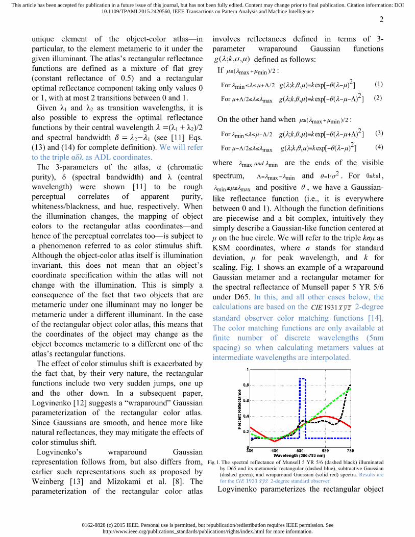
Another difficulty with subtractive Gaussians is that the scaling parameter affects the chromaticity of the resulting Gaussian differently depending on the type. In the case of type G+ changing α has no effect on the resulting chromaticity; however, for type G- changing α results in a different chromaticity. Gaussians of type G- of the same chromaticity will differ in their 𝜙 and σ. Fig. 3 shows an example. Whether it is preferable for a hue descriptor to remain the same for all XYZ of the same chromaticity or instead differ with the scaling can be debated, but it makes little sense for it to do both. In the case of wraparound Gaussians, all XYZ of the same chromaticity are always represented by Gaussians of the same σ and µ.

Fig. 2. Two metameric subtractive Gaussian functions, one of

type G+ (black) and type G- (red). Under D65, both these reflectances have CIE XYZ values (63.69, 64.97, 20.95). Parameters (α, 𝜎, 𝜙) defining these G+ and G- spectra are (0.8670, 93.5557, 621.1427) and (-1.0000, 118.4952, 380.0106), respectively.

Fig. 3. Three G- spectra having the same chromaticity but with

their XYZ differing by a scale factor. Red curve: G- spectrum having XYZ = (77.9114, 79.2585, 20.8546). Dotted blue curve: 0.95 x XYZ. Dashed green curve: 0.9 x XYZ. Parameters (α, 𝜎, 𝜙) defining these three G- spectra are (-1.0000, 38.5005, 469.9995), (-0.8835, 56.2495, 455.2326) and (-0.8922, 74.5022, 436.1658), respectively. Although the three curves appear to intersect at a common point in the plot, they in fact do not.

IV. TESTS AND RESULTS We address two main questions: How well does

the peak wavelength, µ, correlate with hue? And is µ, as a hue descriptor, robust to changes in the illumination? In terms of the first question we compare how well it describes the hues of the Munsell papers, the NCS papers, and the hues Moroney tabulated in a Color Thesaurus [16] that were derived from a large, crowd-sourced, color-naming experiment [17][18]. In terms of the second question, we compare the shift an illuminant change induces in µ and compare it to the shift it induces in CIECAM02 hue. The results show that µ is an accurate hue descriptor that is more robust relative to the illuminant than CIECAM02 hue.

Note that in what follows, the plots are of hue versus log(σ) or hue versus CIECAM02 saturation, but all the analysis is strictly in terms of hue. Possible perceptual correlates of σ will be investigated elsewhere. In the present context, it is simply being used to spread out the hue plots nicely.

In terms of computational requirements, KSM and ADL are very similar. The results reported below are based on the lookup-table-followed-by-optimization approach originally proposed by Godau et al. [19] and require on the order of 60ms per sample. However, Finlayson et al. [20] developed a slightly less accurate, but much faster,

380 480 580 680 7800

0.2

0.4

0.6

0.8

1

Wavelength (380-780 nm)

Perc

ent R

efle

ctan

ce



5

kd-tree method that requires only 0.1ms per sample and is fast enough to use with images.

A. Munsell Dataset As a comparison of KSM µ and CIECAM02 hue

correlates, we consider the set of 1600 papers of the Munsell glossy set. This follows a similar analysis by Logvinenko [11] of his ADL hue correlate λ. We synthesized the XYZ tristimulus values of all 1600 papers based on the Joensuu Color Group spectral measurements [21] under the illuminant C using the

2-degree color matching functions and then computed the corresponding KSM (µ), ADL (λ), and CIECAM02 hues. When calculating the CIECAM02 appearance attributes, we adopted the parameters suggested for the “average surround” condition and full adaptation.

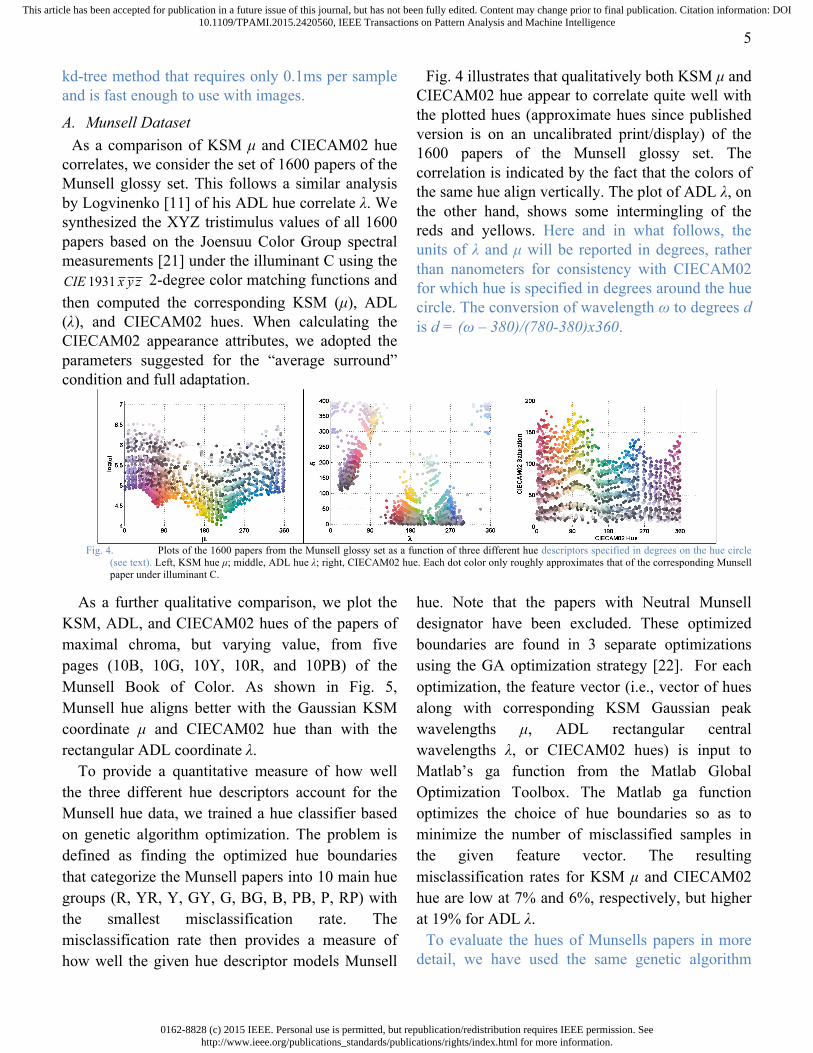
Fig. 4 illustrates that qualitatively both KSM µ and CIECAM02 hue appear to correlate quite well with the plotted hues (approximate hues since published version is on an uncalibrated print/display) of the 1600 papers of the Munsell glossy set. The correlation is indicated by the fact that the colors of the same hue align vertically. The plot of ADL λ, on the other hand, shows some intermingling of the reds and yellows. Here and in what follows, the units of λ and µ will be reported in degrees, rather than nanometers for consistency with CIECAM02 for which hue is specified in degrees around the hue circle. The conversion of wavelength ω to degrees d is d = (ω – 380)/(780-380)x360.

Fig. 4. Plots of the 1600 papers from the Munsell glossy set as a function of three different hue descriptors specified in degrees on the hue circle

(see text). Left, KSM hue µ; middle, ADL hue λ; right, CIECAM02 hue. Each dot color only roughly approximates that of the corresponding Munsell paper under illuminant C.

As a further qualitative comparison, we plot the

KSM, ADL, and CIECAM02 hues of the papers of maximal chroma, but varying value, from five pages (10B, 10G, 10Y, 10R, and 10PB) of the Munsell Book of Color. As shown in Fig. 5, Munsell hue aligns better with the Gaussian KSM coordinate µ and CIECAM02 hue than with the rectangular ADL coordinate λ.

To provide a quantitative measure of how well the three different hue descriptors account for the Munsell hue data, we trained a hue classifier based on genetic algorithm optimization. The problem is defined as finding the optimized hue boundaries that categorize the Munsell papers into 10 main hue groups (R, YR, Y, GY, G, BG, B, PB, P, RP) with the smallest misclassification rate. The misclassification rate then provides a measure of how well the given hue descriptor models Munsell

hue. Note that the papers with Neutral Munsell designator have been excluded. These optimized boundaries are found in 3 separate optimizations using the GA optimization strategy [22]. For each optimization, the feature vector (i.e., vector of hues along with corresponding KSM Gaussian peak wavelengths µ, ADL rectangular central wavelengths λ, or CIECAM02 hues) is input to Matlab’s ga function from the Matlab Global Optimization Toolbox. The Matlab ga function optimizes the choice of hue boundaries so as to minimize the number of misclassified samples in the given feature vector. The resulting misclassification rates for KSM µ and CIECAM02 hue are low at 7% and 6%, respectively, but higher at 19% for ADL λ.

To evaluate the hues of Munsells papers in more detail, we have used the same genetic algorithm

CIE 1931 x y z



6

optimization to determine the optimal hue boundaries for the intermediate Munsell hue classes and measured the corresponding misclassification rates. Fig. 6 shows the misclassification rates for the intermediate Munsell hue designators which are red (Munsell hues R, 2.5R, 5R, 7.5R, and 10R) yellow-red (YR, 2.5YR, …), yellow, green-yellow, green, blue-green, blue, purple-blue, purple, and red-purple papers. The average misclassification rate across all the hues combined is 31% for KSM µ versus 41% for CIECAM02 hue. B. NCS Dataset

The Natural Color System (NCS) [23] provides another set of hue data. In the NCS notation hue is defined in terms of the percentage of the distance between the neighboring pairs of the ‘elementary’

hues red, yellow, green, blue. The two other components of the NCS notation specify the blackness and chromaticness. We carried out a sequence of tests using the NCS data that are similar to those described above using the Munsell data. The plot of the 1950 NCS papers analogous to Fig. 4 is qualitatively very similar and therefore is not included here. As in the case of the Munsell papers, KSM µ and CIECAM02 hue show a very good correlation with NCS hue, while ADL correlates, but not as unambiguously.

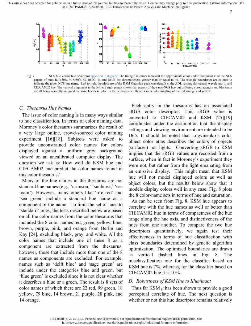
Fig. 7 plots the NCS papers of NCS hues R, Y50R, Y, G50Y, G, B50G, B, and R50B as a function of the KSM µ, ADL λ and CIECAM02 hue descriptors in a manner analogous to that of Fig. 5 for the Munsell papers.

Fig. 5. Munsell hue versus hue descriptor specified in degrees. The triangle interiors represent the approximate color under illuminant C of the

Munsell papers of different Munsell value, each at maximal chroma for the given value, for the five hues 10B, 10G, 10Y, 10R, and 10PB. The triangle boundaries are colored with the maximal chroma for the given Munsell hue. Left to right the plots are of the KSM Gaussian peak wavelength µ, the ADL rectangular central wavelength λ, and CIECAM02 hue. The vertical alignment in the left and right panels shows that papers of the same Munsell hue but differing value are all being assigned the same hue descriptor. In the central panel, there is some mingling of the red with the yellow and of the blue with the purple hues.

Fig. 6. Hue misclassification rate for KSM µ (grey) versus CIECAM hue (black) over papers of the intermediate Munsell hues. The average misclassification rate for all the hues combined is 31% for KSM µ versus 41% for CIECAM02 hue.

0.00%

10.00%

20.00%

30.00%

40.00%

50.00%

60.00%

70.00%

80.00%

90.00%

R R R R YR YR YR YR Y Y Y Y GY GY GY GY G G G G BG BG BG BG B B B B PB PB PB PB P P P P RP RP RP RP

2.5 5 7.5 10 2.5 5 7.5 10 2.5 5 7.5 10 2.5 5 7.5 10 2.5 5 7.5 10 2.5 5 7.5 10 2.5 5 7.5 10 2.5 5 7.5 10 2.5 5 7.5 10 2.5 5 7.5 10



7

Fig. 7. NCS hue versus hue descriptor specified in degrees. The triangle interiors represent the approximate color under illuminant C of the NCS

papers of hues R, Y50R, Y, G50Y, G, B50G, B, and R50B for chromaticness greater than or equal to 40. The triangle boundaries are colored to indicate the given NCS hue name. Left to right the plots are of the KSM Gaussian peak wavelength µ, the ADL rectangular central wavelength λ, and CIECAM02 hue. The vertical alignment in the left and right panels shows that papers of the same NCS hue but differing chromaticness and blackness are all being correctly assigned the same hue descriptor. In the central panel, there is some intermingling of the red, orange and yellow.

C. Thesaurus Hue Names The issue of color naming is in many ways similar

to hue classification. In terms of color naming data, Moroney’s color thesaurus summarizes the result of a very large online, crowd-sourced color naming experiment [16][18]. Subjects were asked to provide unconstrained color names for colors displayed against a uniform grey background viewed on an uncalibrated computer display. The question we ask is: How well do KSM hue and CIECAM02 hue predict the color names found in this color thesaurus?

Many of the hue names in the thesaurus are not standard hue names (e.g., ‘crimson,’ ‘sunburst,’ ‘sea foam’). However, many others like ‘fire red’ and ‘sea green’ include a standard hue name as a component of the name. To limit the set of hues to ‘standard’ ones, the tests described below are based on all the color names from the color thesaurus that included the 8 color names red, green, yellow, blue, brown, purple, pink, and orange from Berlin and Kay [24], excluding black, gray, and white. All the color names that include one of these 8 as a component are extracted from the thesaurus; however, those that include more than one of the 8 names as components are excluded. For example, names such as ‘delft blue’ and ‘sage green’ are include under the categories blue and green, but ‘blue green’ is excluded since it is not clear whether it describes a blue or a green. The result is 8 sets of color names of which there are 22 red, 99 green, 18 yellow, 79 blue, 14 brown, 21 purple, 28 pink, and 14 orange.

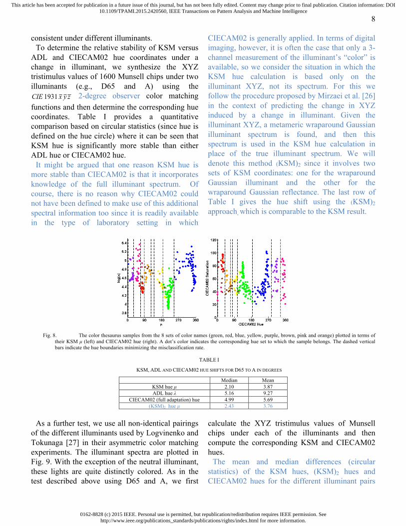
Each entry in the thesaurus has an associated sRGB color descriptor. This sRGB value is converted to CIECAM02 and KSM [25][19] coordinates under the assumption that the display settings and viewing environment are intended to be D65. It should be noted that Logvinenko’s color object color atlas describes the colors of objects (surfaces) not lights. Converting sRGB to KSM implies that the sRGB values are recorded from a surface, when in fact in Moroney’s experiment they were not, but rather from the light emanating from an emissive display. This might mean that KSM hue will not model displayed colors as well as object colors, but the results below show that it models display colors well in any case. Fig. 8 plots the 8 color-name sets in terms of hue and saturation.

As can be seen from Fig. 8, KSM hue appears to correlate with the hue names as well or better than CIECAM02 hue in terms of compactness of the hue range along the hue axis, and distinctiveness of the hues from one another. To compare the two hue descriptors quantitatively, we again test their effectiveness in terms of hue classification with class boundaries determined by genetic algorithm optimization. The optimized boundaries are drawn as vertical dashed lines in Fig. 8. The misclassification rate for the classifier based on KSM hue is 7%, whereas, for the classifier based on CIECAM02 hue it is 10%.

D. Robustness of KSM Hue to Illuminant Thus far KSM µ has been shown to provide a good

perceptual correlate of hue. The next question is whether or not this hue descriptor remains relatively



8

consistent under different illuminants. To determine the relative stability of KSM versus

ADL and CIECAM02 hue coordinates under a change in illuminant, we synthesize the XYZ tristimulus values of 1600 Munsell chips under two illuminants (e.g., D65 and A) using the

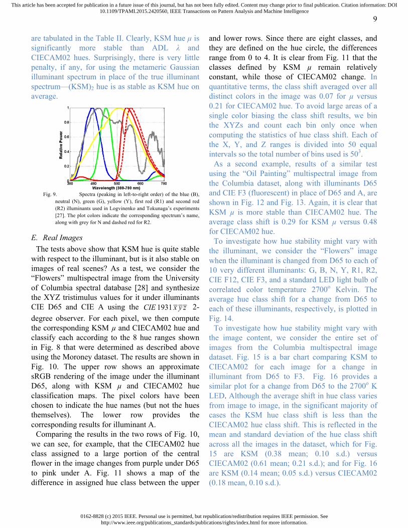
2-degree observer color matching functions and then determine the corresponding hue coordinates. Table I provides a quantitative comparison based on circular statistics (since hue is defined on the hue circle) where it can be seen that KSM hue is significantly more stable than either ADL hue or CIECAM02 hue.

It might be argued that one reason KSM hue is more stable than CIECAM02 is that it incorporates knowledge of the full illuminant spectrum. Of course, there is no reason why CIECAM02 could not have been defined to make use of this additional spectral information too since it is readily available in the type of laboratory setting in which

CIECAM02 is generally applied. In terms of digital imaging, however, it is often the case that only a 3-channel measurement of the illuminant’s “color” is available, so we consider the situation in which the KSM hue calculation is based only on the illuminant XYZ, not its spectrum. For this we follow the procedure proposed by Mirzaei et al. [26] in the context of predicting the change in XYZ induced by a change in illuminant. Given the illuminant XYZ, a metameric wraparound Gaussian illuminant spectrum is found, and then this spectrum is used in the KSM hue calculation in place of the true illuminant spectrum. We will denote this method (KSM)2 since it involves two sets of KSM coordinates: one for the wraparound Gaussian illuminant and the other for the wraparound Gaussian reflectance. The last row of Table I gives the hue shift using the (KSM)2

approach, which is comparable to the KSM result.

Fig. 8. The color thesaurus samples from the 8 sets of color names (green, red, blue, yellow, purple, brown, pink and orange) plotted in terms of

their KSM µ (left) and CIECAM02 hue (right). A dot’s color indicates the corresponding hue set to which the sample belongs. The dashed vertical bars indicate the hue boundaries minimizing the misclassification rate.

TABLE I

KSM, ADL AND CIECAM02 HUE SHIFTS FOR D65 TO A IN DEGREES

Median Mean KSM hue µ 2.10 3.87 ADL hue λ 5.16 9.27

CIECAM02 (full adaptation) hue 4.99 5.69 (KSM)2 hue µ 2.43 3.76

As a further test, we use all non-identical pairings

of the different illuminants used by Logvinenko and Tokunaga [27] in their asymmetric color matching experiments. The illuminant spectra are plotted in Fig. 9. With the exception of the neutral illuminant, these lights are quite distinctly colored. As in the test described above using D65 and A, we first

calculate the XYZ tristimulus values of Munsell chips under each of the illuminants and then compute the corresponding KSM and CIECAM02 hues.

The mean and median differences (circular statistics) of the KSM hues, (KSM)2 hues and CIECAM02 hues for the different illuminant pairs

CIE 1931 x y z



9

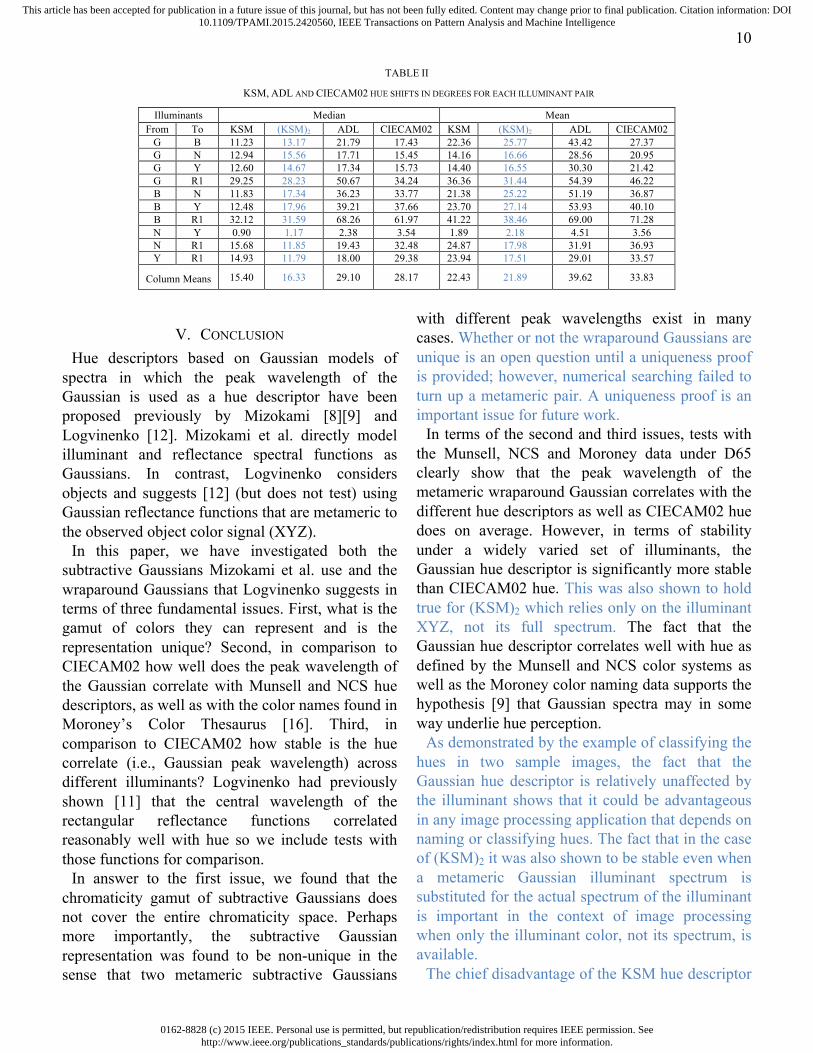
are tabulated in the Table II. Clearly, KSM hue µ is significantly more stable than ADL λ and CIECAM02 hues. Surprisingly, there is very little penalty, if any, for using the metameric Gaussian illuminant spectrum in place of the true illuminant spectrum—(KSM)2 hue is as stable as KSM hue on average.

Fig. 9. Spectra (peaking in left-to-right order) of the blue (B),

neutral (N), green (G), yellow (Y), first red (R1) and second red (R2) illuminants used in Logvinenko and Tokunaga’s experiments [27]. The plot colors indicate the corresponding spectrum’s name, along with grey for N and dashed red for R2.

E. Real Images The tests above show that KSM hue is quite stable

with respect to the illuminant, but is it also stable on images of real scenes? As a test, we consider the “Flowers” multispectral image from the University of Columbia spectral database [28] and synthesize the XYZ tristimulus values for it under illuminants CIE D65 and CIE A using the 2-degree observer. For each pixel, we then compute the corresponding KSM µ and CIECAM02 hue and classify each according to the 8 hue ranges shown in Fig. 8 that were determined as described above using the Moroney dataset. The results are shown in Fig. 10. The upper row shows an approximate sRGB rendering of the image under the illuminant D65, along with KSM µ and CIECAM02 hue classification maps. The pixel colors have been chosen to indicate the hue names (but not the hues themselves). The lower row provides the corresponding results for illuminant A.

Comparing the results in the two rows of Fig. 10, we can see, for example, that the CIECAM02 hue class assigned to a large portion of the central flower in the image changes from purple under D65 to pink under A. Fig. 11 shows a map of the difference in assigned hue class between the upper

and lower rows. Since there are eight classes, and they are defined on the hue circle, the differences range from 0 to 4. It is clear from Fig. 11 that the classes defined by KSM µ remain relatively constant, while those of CIECAM02 change. In quantitative terms, the class shift averaged over all distinct colors in the image was 0.07 for µ versus 0.21 for CIECAM02 hue. To avoid large areas of a single color biasing the class shift results, we bin the XYZs and count each bin only once when computing the statistics of hue class shift. Each of the X, Y, and Z ranges is divided into 50 equal intervals so the total number of bins used is 503.

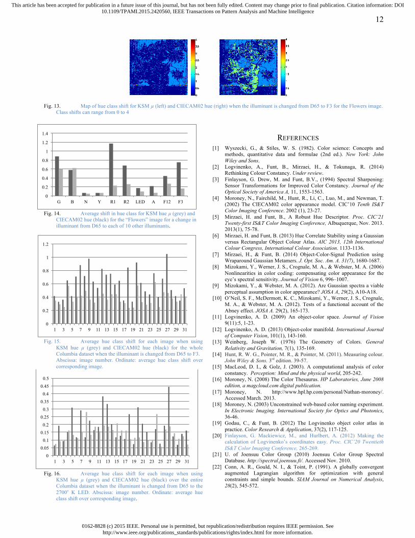
As a second example, results of a similar test using the “Oil Painting” multispectral image from the Columbia dataset, along with illuminants D65 and CIE F3 (fluorescent) in place of D65 and A, are shown in Fig. 12 and Fig. 13. Again, it is clear that KSM µ is more stable than CIECAM02 hue. The average class shift is 0.29 for KSM µ versus 0.48 for CIECAM02 hue.

To investigate how hue stability might vary with the illuminant, we consider the “Flowers” image when the illuminant is changed from D65 to each of 10 very different illuminants: G, B, N, Y, R1, R2, CIE F12, CIE F3, and a standard LED light bulb of correlated color temperature 2700o Kelvin. The average hue class shift for a change from D65 to each of these illuminants, respectively, is plotted in Fig. 14.

To investigate how hue stability might vary with the image content, we consider the entire set of images from the Columbia multispectral image dataset. Fig. 15 is a bar chart comparing KSM to CIECAM02 for each image for a change in illuminant from D65 to F3. Fig. 16 provides a similar plot for a change from D65 to the 2700o K LED. Although the average shift in hue class varies from image to image, in the significant majority of cases the KSM hue class shift is less than the CIECAM02 hue class shift. This is reflected in the mean and standard deviation of the hue class shift across all the images in the dataset, which for Fig. 15 are KSM (0.38 mean; 0.10 s.d.) versus CIECAM02 (0.61 mean; 0.21 s.d.); and for Fig. 16 are KSM (0.14 mean; 0.05 s.d.) versus CIECAM02 (0.18 mean, 0.10 s.d.).

CIE 1931 x y z



10

TABLE II

KSM, ADL AND CIECAM02 HUE SHIFTS IN DEGREES FOR EACH ILLUMINANT PAIR

Illuminants Median Mean From To KSM (KSM)2 ADL CIECAM02 KSM (KSM)2 ADL CIECAM02

G B 11.23 13.17 21.79 17.43 22.36 25.77 43.42 27.37 G N 12.94 15.56 17.71 15.45 14.16 16.66 28.56 20.95 G Y 12.60 14.67 17.34 15.73 14.40 16.55 30.30 21.42 G R1 29.25 28.23 50.67 34.24 36.36 31.44 54.39 46.22 B N 11.83 17.34 36.23 33.77 21.38 25.22 51.19 36.87 B Y 12.48 17.96 39.21 37.66 23.70 27.14 53.93 40.10 B R1 32.12 31.59 68.26 61.97 41.22 38.46 69.00 71.28 N Y 0.90 1.17 2.38 3.54 1.89 2.18 4.51 3.56 N R1 15.68 11.85 19.43 32.48 24.87 17.98 31.91 36.93 Y R1 14.93 11.79 18.00 29.38 23.94 17.51 29.01 33.57

Column Means 15.40 16.33 29.10 28.17 22.43 21.89 39.62 33.83

V. CONCLUSION Hue descriptors based on Gaussian models of

spectra in which the peak wavelength of the Gaussian is used as a hue descriptor have been proposed previously by Mizokami [8][9] and Logvinenko [12]. Mizokami et al. directly model illuminant and reflectance spectral functions as Gaussians. In contrast, Logvinenko considers objects and suggests [12] (but does not test) using Gaussian reflectance functions that are metameric to the observed object color signal (XYZ).

In this paper, we have investigated both the subtractive Gaussians Mizokami et al. use and the wraparound Gaussians that Logvinenko suggests in terms of three fundamental issues. First, what is the gamut of colors they can represent and is the representation unique? Second, in comparison to CIECAM02 how well does the peak wavelength of the Gaussian correlate with Munsell and NCS hue descriptors, as well as with the color names found in Moroney’s Color Thesaurus [16]. Third, in comparison to CIECAM02 how stable is the hue correlate (i.e., Gaussian peak wavelength) across different illuminants? Logvinenko had previously shown [11] that the central wavelength of the rectangular reflectance functions correlated reasonably well with hue so we include tests with those functions for comparison.

In answer to the first issue, we found that the chromaticity gamut of subtractive Gaussians does not cover the entire chromaticity space. Perhaps more importantly, the subtractive Gaussian representation was found to be non-unique in the sense that two metameric subtractive Gaussians

with different peak wavelengths exist in many cases. Whether or not the wraparound Gaussians are unique is an open question until a uniqueness proof is provided; however, numerical searching failed to turn up a metameric pair. A uniqueness proof is an important issue for future work.

In terms of the second and third issues, tests with the Munsell, NCS and Moroney data under D65 clearly show that the peak wavelength of the metameric wraparound Gaussian correlates with the different hue descriptors as well as CIECAM02 hue does on average. However, in terms of stability under a widely varied set of illuminants, the Gaussian hue descriptor is significantly more stable than CIECAM02 hue. This was also shown to hold true for (KSM)2 which relies only on the illuminant XYZ, not its full spectrum. The fact that the Gaussian hue descriptor correlates well with hue as defined by the Munsell and NCS color systems as well as the Moroney color naming data supports the hypothesis [9] that Gaussian spectra may in some way underlie hue perception.

As demonstrated by the example of classifying the hues in two sample images, the fact that the Gaussian hue descriptor is relatively unaffected by the illuminant shows that it could be advantageous in any image processing application that depends on naming or classifying hues. The fact that in the case of (KSM)2 it was also shown to be stable even when a metameric Gaussian illuminant spectrum is substituted for the actual spectrum of the illuminant is important in the context of image processing when only the illuminant color, not its spectrum, is available.

The chief disadvantage of the KSM hue descriptor



11

is that it is more costly to compute than CIECAM02 hue, a problem that can be easily addressed by appropriate use of lookup tables and kd-trees [20]. Although very important, hue is only one perceptual

dimension of color. Future work will involve using the other KSM parameters in modeling dimensions such as purity/saturation.

Fig. 10. Hue classification using KSM µ versus CIECAM02 hue of the Flowers image from the Columbia University spectral database [28]. First

and second rows depict the classification results for illuminants D65 and A, respectively. Left panel: Approximate sRGB rendering of the image. Middle: segmentation based on µ. Right: classification based on CIECAM02 hue. Each pixel is colored to roughly represent the hue name assigned to it.

Fig. 11. Map of hue class shift for µ (left) and CIECAM02 hue (right) when the illuminant is changed from D65 to A. Class shifts can range from 0

to 4.

Fig. 12. Hue classification using KSM µ versus CIECAM02 hue of the Flowers image from the Columbia University spectral database [28]. First

and second rows depict the classification results for illuminants D65 and F3, respectively. Left panel: Approximate sRGB rendering of the image. Middle: classification based on µ. Right: classification based on CIECAM02 hue. Each pixel is colored to roughly represent the hue name assigned to it.



12

Fig. 13. Map of hue class shift for KSM µ (left) and CIECAM02 hue (right) when the illuminant is changed from D65 to F3 for the Flowers image.

Class shifts can range from 0 to 4

Fig. 14. Average shift in hue class for KSM hue µ (grey) and

CIECAM02 hue (black) for the “Flowers” image for a change in illuminant from D65 to each of 10 other illuminants.

Fig. 15. Average hue class shift for each image when using

KSM hue µ (grey) and CIECAM02 hue (black) for the whole Columbia dataset when the illuminant is changed from D65 to F3. Abscissa: image number. Ordinate: average hue class shift over corresponding image.

Fig. 16. Average hue class shift for each image when using

KSM hue µ (grey) and CIECAM02 hue (black) over the entire Columbia dataset when the illuminant is changed from D65 to the 2700o K LED. Abscissa: image number. Ordinate: average hue class shift over corresponding image.

REFERENCES [1] Wyszecki, G., & Stiles, W. S. (1982). Color science: Concepts and

methods, quantitative data and formulae (2nd ed.). New York: John Wiley and Sons.

[2] Logvinenko, A., Funt, B., Mirzaei, H., & Tokunaga, R. (2014) Rethinking Colour Constancy. Under review.

[3] Finlayson, G. Drew, M. and Funt, B.V., (1994) Spectral Sharpening: Sensor Transformations for Improved Color Constancy. Journal of the Optical Society of America A, 11, 1553-1563.

[4] Moroney, N., Fairchild, M., Hunt, R., Li, C., Luo, M., and Newman, T. (2002) The CIECAM02 color appearance model. CIC’10 Tenth IS&T Color Imaging Conference. 2002 (1), 23-27.

[5] Mirzaei, H. and Funt, B., A Robust Hue Descriptor. Proc. CIC’21 Twenty-first IS&T Color Imaging Conference, Albuquerque, Nov. 2013. 2013(1), 75-78.

[6] Mirzaei, H. and Funt, B. (2013) Hue Correlate Stability using a Gaussian versus Rectangular Object Colour Atlas. AIC 2013, 12th International Colour Congress, International Colour Association. 1133-1136.

[7] Mirzaei, H., & Funt, B. (2014) Object-Color-Signal Prediction using Wraparound Gaussian Metamers. J. Opt. Soc. Am. A. 31(7), 1680-1687.

[8] Mizokami, Y., Werner, J. S., Crognale, M. A., & Webster, M. A. (2006) Nonlinearities in color coding: compensating color appearance for the eye’s spectral sensitivity. Journal of Vision 6, 996–1007.

[9] Mizokami, Y., & Webster, M. A. (2012). Are Gaussian spectra a viable perceptual assumption in color appearance? JOSA A, 29(2), A10-A18.

[10] O’Neil, S. F., McDermott, K. C., Mizokami, Y., Werner, J. S., Crognale, M. A., & Webster, M. A. (2012). Tests of a functional account of the Abney effect. JOSA A. 29(2), 165-173.

[11] Logvinenko, A. D. (2009) An object-color space. Journal of Vision 9(11):5, 1-23.

[12] Logvinenko, A. D. (2013) Object-color manifold. International Journal of Computer Vision, 101(1), 143-160.

[13] Weinberg, Joseph W. (1976) The Geometry of Colors. General Relativity and Gravitation, 7(1), 135-169.

[14] Hunt, R. W. G., Pointer, M. R., & Pointer, M. (2011). Measuring colour. John Wiley & Sons. 3rd edition. 39-57.

[15] MacLeod, D. I., & Golz, J. (2003). A computational analysis of color constancy. Perception: Mind and the physical world, 205-242.

[16] Moroney, N. (2008) The Color Thesaurus. HP Laboratories, June 2008 edition, a magcloud.com digital publication.

[17] Moroney, N. http://www.hpl.hp.com/personal/Nathan-moroney/. Accessed March. 2013.

[18] Moroney, N. (2003) Unconstrained web-based color naming experiment. In Electronic Imaging. International Society for Optics and Photonics, 36-46.

[19] Godau, C., & Funt, B. (2012) The Logvinenko object color atlas in practice. Color Research & Application, 37(2), 117-125.

[20] Finlayson, G. Mackiewicz, M., and Hurlbert, A. (2012) Making the calculation of Logvinenko’s coordinates easy. Proc. CIC’20 Twentieth IS&T Color Imaging Conference, 265-269.

[21] U. of Joensuu Color Group (2010) Joensuu Color Group Spectral Database. http://spectral.joensuu.fi/. Accessed Nov. 2010.

[22] Conn, A. R., Gould, N. I., & Toint, P. (1991). A globally convergent augmented Lagrangian algorithm for optimization with general constraints and simple bounds. SIAM Journal on Numerical Analysis, 28(2), 545-572.

0

0.2

0.4

0.6

0.8

1

1.2

1.4

G B N Y R1 R2 LED A F12 F3

0

0.2

0.4

0.6

0.8

1

1.2

1 3 5 7 9 11 13 15 17 19 21 23 25 27 29 31

0 0.05 0.1

0.15 0.2

0.25 0.3

0.35 0.4

0.45 0.5

1 3 5 7 9 11 13 15 17 19 21 23 25 27 29 31



13

[23] Hård, A., & Sivik, L. (1981). NCS—Natural Color System: a Swedish standard for color notation. Color Research & Application. 6(3), 129-138.

[24] Berlin, B., & Kay, P. (1991) Basic color terms: Their universality and evolution. Univ. of California Press.

[25] Funt, B., & Mirzaei, H. (2011) Intersecting Colour Manifolds. Proc. CIC’19 Nineteenth IS&T Color Imaging Conference. 2011(1), 166-170.

[26] Mirzaei, H. and Funt. B., (2014) Gaussian Illuminants and Reflectances for Colour Signal Prediction, Proc. CIC’22 Twenty Second IS&T Color Imaging Conference, 212-216.

[27] Logvinenko, A. D., & Tokunaga, R. (2011). Colour constancy as measured by least dissimilar matching. Seeing and Perceiving, 24(5), 407-452.

[28] Yasuma, F., Mitsunaga, T., Iso, D., & Nayar, S. K. (2010). Generalized assorted pixel camera: postcapture control of resolution, dynamic range, and spectrum. Image Processing, IEEE Transactions on, 19(9), 2241-2253.

Author Biographies Hamidreza Mirzaei received his M.Sc. from the School of Computing Science at Simon Fraser University (SFU) in 2011. He is currently a Ph.D. candidate in the computational vision lab at SFU where his research spans different areas of color vision. He has published several articles on color imaging and computational vision.

Brian Funt is Professor of Computing Science at Simon Fraser University where he has been since 1980. He obtained his Ph.D. from the University of British Columbia in 1976. His research focus is on computational approaches to modeling and understanding color.

Documents

Gaussian Based Hue Descriptors - Computing Science ...funt/Mirzaei+Funt_GaussianHue_PAMI2015.pdfpseudo-color atlas as the representation of hue. Such Gaussian-like reflectances have