Embed Size (px)
Citation preview
Gaussian Process Optimization in the Bandit Setting:No Regret and Experimental Design
Niranjan SrinivasCalifornia Institute of Technology
Andreas KrauseCalifornia Institute of Technology
Sham M. KakadeUniversity of Pennsylvania
Matthias SeegerSaarland University
Abstract
Many applications require optimizing an un-known, noisy function that is expensive toevaluate. We formalize this task as a multi-armed bandit problem, where the payoff functionis either sampled from a Gaussian process (GP)or has low RKHS norm. We resolve the impor-tant open problem of deriving regret bounds forthis setting, which imply novel convergence ratesfor GP optimization. We analyze GP-UCB, anintuitive upper-confidence based algorithm, andbound its cumulative regret in terms of maximalinformation gain, establishing a novel connectionbetween GP optimization and experimental de-sign. Moreover, by bounding the latter in termsof operator spectra, we obtain explicit sublinearregret bounds for many commonly used covari-ance functions. In some important cases, ourbounds have surprisingly weak dependence onthe dimensionality. In our experiments on realsensor data, GP-UCB compares favorably withother heuristical GP optimization approaches.
1. Introduction
In most stochastic optimization settings, evaluatingthe unknown function is expensive, and samplingis to be minimized. Examples include choosingadvertisements in sponsored search to maximizeprofit in a click-through model (Pandey & Olston,2007) or learning optimal control strategies for robots(Lizotte et al., 2007). Predominant approachesto this problem include the multi-armed banditparadigm (Robbins, 1952), where the goal is tomaximize cumulative reward by optimally balancingexploration and exploitation, and experimental design(Chaloner & Verdinelli, 1995), where the functionis to be explored globally with as few evaluationsas possible, for example by maximizing information
1This is the longer version of our paper in ICML 2010;see Srinivas et al. (2010)
gain. The challenge in both approaches is twofold: wehave to estimate an unknown function f from noisysamples, and we must optimize our estimate over somehigh-dimensional input space. For the former, muchprogress has been made in machine learning throughkernel methods and Gaussian process (GP) models(Rasmussen & Williams, 2006), where smoothnessassumptions about f are encoded through the choiceof kernel in a flexible nonparametric fashion. BeyondEuclidean spaces, kernels can be defined on diversedomains such as spaces of graphs, sets, or lists.
We are concerned with GP optimization in the multi-armed bandit setting, where f is sampled from a GPdistribution or has low “complexity” measured interms of its RKHS norm under some kernel. We pro-vide the first sublinear regret bounds in this nonpara-metric setting, which imply convergence rates for GPoptimization. In particular, we analyze the GaussianProcess Upper Confidence Bound (GP-UCB) algo-rithm, a simple and intuitive Bayesian method (Aueret al., 2002; Auer, 2002; Dani et al., 2008). Whileobjectives are different in the multi-armed banditand experimental design paradigm, our results drawa close technical connection between them: our regretbounds come in terms of an information gain quantity,measuring how fast f can be learned in an informationtheoretic sense. The submodularity of this functionallows us to prove sharp regret bounds for particularcovariance functions, which we demonstrate for com-monly used Squared Exponential and Matern kernels.
Related Work. Our work generalizes stochasticlinear optimization in a bandit setting, where theunknown function comes from a finite-dimensionallinear space. GPs are nonlinear random functions,which can be represented in an infinite-dimensionallinear space. For the standard linear setting, Daniet al. (2008) provide a near-complete characterization
1
arX
iv:0
912.
3995
v4 [
cs.L
G]
9 J
un 2
010

(also see Auer 2002; Dani et al. 2007; Abernethy et al.2008; Rusmevichientong & Tsitsiklis 2008), explicitlydependent on the dimensionality. In the GP setting,the challenge is to characterize complexity in a differ-ent manner, through properties of the kernel function.Our technical contributions are twofold: first, weshow how to analyze the nonlinear setting by focusingon the concept of information gain, and second, weexplicitly bound this information gain measure usingthe concept of submodularity (Nemhauser et al.,1978) and knowledge about kernel operator spectra.
Kleinberg et al. (2008) provide regret bounds un-der weaker and less configurable assumptions (onlyLipschitz-continuity w.r.t. a metric is assumed;Bubeck et al. 2008 consider arbitrary topologicalspaces), which however degrade rapidly with the di-
mensionality of the problem (Ω(Td+1d+2 )). In practice,
linearity w.r.t. a fixed basis is often too stringentan assumption, while Lipschitz-continuity can be toocoarse-grained, leading to poor rate bounds. AdoptingGP assumptions, we can model levels of smoothness ina fine-grained way. For example, our rates for the fre-quently used Squared Exponential kernel, enforcing ahigh degree of smoothness, have weak dependence onthe dimensionality: O(
√T (log T )d+1) (see Fig. 1).
There is a large literature on GP (response surface)optimization. Several heuristics for trading off explo-ration and exploitation in GP optimization have beenproposed (such as Expected Improvement, Mockuset al. 1978, and Most Probable Improvement, Mockus1989) and successfully applied in practice (c.f., Lizotteet al. 2007). Brochu et al. (2009) provide a comprehen-sive review of and motivation for Bayesian optimiza-tion using GPs. The Efficient Global Optimization(EGO) algorithm for optimizing expensive black-boxfunctions is proposed by Jones et al. (1998) and ex-tended to GPs by Huang et al. (2006). Little is knownabout theoretical performance of GP optimization.While convergence of EGO is established by Vazquez& Bect (2007), convergence rates have remained elu-sive. Grunewalder et al. (2010) consider the pure ex-ploration problem for GPs, where the goal is to find theoptimal decision over T rounds, rather than maximizecumulative reward (with no exploration/exploitationdilemma). They provide sharp bounds for this explo-ration problem. Note that this methodology would notlead to bounds for minimizing the cumulative regret.Our cumulative regret bounds translate to the firstperformance guarantees (rates) for GP optimization.
Summary. Our main contributions are:
• We analyze GP-UCB, an intuitive algorithm forGP optimization, when the function is either sam-
Kernel Linear kernel
RBF Matérn kernel Regret RT
T (log T )d+1
Tν+d(d+1)2ν+d(d+1)d
√T
Figure 1. Our regret bounds (up to polylog factors) for lin-ear, radial basis, and Matern kernels — d is the dimension,T is the time horizon, and ν is a Matern parameter.
pled from a known GP, or has low RKHS norm.
• We bound the cumulative regret for GP-UCB interms of the information gain due to sampling,establishing a novel connection between experi-mental design and GP optimization.
• By bounding the information gain for popularclasses of kernels, we establish sublinear regretbounds for GP optimization for the first time.Our bounds depend on kernel choice and param-eters in a fine-grained fashion.
• We evaluate GP-UCB on sensor network data,demonstrating that it compares favorably to ex-isting algorithms for GP optimization.
2. Problem Statement and Background
Consider the problem of sequentially optimizing an un-known reward function f : D → R: in each round t, wechoose a point xt ∈ D and get to see the function valuethere, perturbed by noise: yt = f(xt)+ εt. Our goal is
to maximize the sum of rewards∑Tt=1 f(xt), thus to
perform essentially as well as x∗ = argmaxx∈D f(x)(as rapidly as possible). For example, we might wantto find locations of highest temperature in a buildingby sequentially activating sensors in a spatial networkand regressing on their measurements. D consists ofall sensor locations, f(x) is the temperature at x, andsensor accuracy is quantified by the noise variance.Each activation draws battery power, so we want tosample from as few sensors as possible.
Regret. A natural performance metric in this con-text is cumulative regret, the loss in reward due to notknowing f ’s maximum points beforehand. Supposethe unknown function is f , its maximum point1
x∗ = argmaxx∈D f(x). For our choice xt in roundt, we incur instantaneous regret rt = f(x∗) − f(xt).The cumulative regret RT after T rounds is the sumof instantaneous regrets: RT =
∑Tt=1 rt. A desirable
asymptotic property of an algorithm is to be no-regret :limT→∞RT /T = 0. Note that neither rt nor RT areever revealed to the algorithm. Bounds on the averageregret RT /T translate to convergence rates for GPoptimization: the maximum maxt≤T f(xt) in the firstT rounds is no further from f(x∗) than the average.
1 x∗ need not be unique; only f(x∗) occurs in the regret.
2.1. Gaussian Processes and RKHS’s
Gaussian Processes. Some assumptions on f arerequired to guarantee no-regret. While rigid paramet-ric assumptions such as linearity may not hold in prac-tice, a certain degree of smoothness is often warranted.In our sensor network, temperature readings at closebylocations are highly correlated (see Figure 2(a)). Wecan enforce implicit properties like smoothness with-out relying on any parametric assumptions, modelingf as a sample from a Gaussian process (GP): a col-lection of dependent random variables, one for eachx ∈ D, every finite subset of which is multivariateGaussian distributed in an overall consistent way (Ras-mussen & Williams, 2006). A GP (µ(x), k(x,x′)) isspecified by its mean function µ(x) = E[f(x)] andcovariance (or kernel) function k(x,x′) = E[(f(x) −µ(x))(f(x′) − µ(x′))]. For GPs not conditioned ondata, we assume2 that µ ≡ 0. Moreover, we restrictk(x,x) ≤ 1, x ∈ D, i.e., we assume bounded variance.By fixing the correlation behavior, the covariance func-tion k encodes smoothness properties of sample func-tions f drawn from the GP. A range of commonly usedkernel functions is given in Section 5.2.
In this work, GPs play multiple roles. First, some ofour results hold when the unknown target function is asample from a known GP distribution GP(0, k(x,x′)).Second, the Bayesian algorithm we analyze generallyuses GP(0, k(x,x′)) as prior distribution over f . Amajor advantage of working with GPs is the exis-tence of simple analytic formulae for mean and co-variance of the posterior distribution, which allowseasy implementation of algorithms. For a noisy sam-ple yT = [y1 . . . yT ]T at points AT = x1, . . . ,xT ,yt = f(xt)+εt with εt ∼ N(0, σ2) i.i.d. Gaussian noise,the posterior over f is a GP distribution again, withmean µT (x), covariance kT (x,x′) and variance σ2
T (x):
µT (x) = kT (x)T (KT + σ2I)−1yT , (1)
kT (x,x′) = k(x,x′)− kT (x)T (KT + σ2I)−1kT (x′),
σ2T (x) = kT (x,x), (2)
where kT (x) = [k(x1,x) . . . k(xT ,x)]T and KT isthe positive definite kernel matrix [k(x,x′)]x,x′∈AT
.
RKHS. Instead of the Bayes case, where f is sam-pled from a GP prior, we also consider the more ag-nostic case where f has low “complexity” as measuredunder an RKHS norm (and distribution free assump-tions on the noise process). The notion of reproduc-ing kernel Hilbert spaces (RKHS, Wahba 1990) is in-timately related to GPs and their covariance func-tions k(x,x′). The RKHS Hk(D) is a complete sub-space of L2(D) of nicely behaved functions, with an
2This is w.l.o.g. (Rasmussen & Williams, 2006).
inner product 〈·, ·〉k obeying the reproducing property:〈f, k(x, ·)〉k = f(x) for all f ∈ Hk(D). It is literallyconstructed by completing the set of mean functionsµT for all possible T , xt, and yT . The inducedRKHS norm ‖f‖k =
√〈f, f〉k measures smoothness of
f w.r.t. k: in much the same way as k1 would generatesmoother samples than k2 as GP covariance functions,‖·‖k1 assigns larger penalties than ‖·‖k2 . 〈·, ·〉k can beextended to all of L2(D), in which case ‖f‖k < ∞ ifff ∈ Hk(D). For most kernels discussed in Section 5.2,members of Hk(D) can uniformly approximate anycontinuous function on any compact subset of D.
2.2. Information Gain & Experimental Design
One approach to maximizing f is to first choosepoints xt so as to estimate the function globallywell, then play the maximum point of our estimate.How can we learn about f as rapidly as possible?This question comes down to Bayesian ExperimentalDesign (henceforth “ED”; see Chaloner & Verdinelli1995), where the informativeness of a set of samplingpoints A ⊂ D about f is measured by the informationgain (c.f., Cover & Thomas 1991), which is the mutualinformation between f and observations yA = fA+εAat these points:
I(yA; f) = H(yA)−H(yA|f), (3)
quantifying the reduction in uncertainty about ffrom revealing yA. Here, fA = [f(x)]x∈A andεA ∼ N(0, σ2I). For a Gaussian, H(N(µ,Σ)) =12 log |2πeΣ|, so that in our setting I(yA; f) =I(yA;fA) = 1
2 log |I + σ−2KA|, where KA =[k(x,x′)]x,x′∈A. While finding the information gainmaximizer among A ⊂ D, |A| ≤ T is NP-hard (Koet al., 1995), it can be approximated by an efficientgreedy algorithm. If F (A) = I(yA; f), this algorithmpicks xt = argmaxx∈D F (At−1∪x) in round t, whichcan be shown to be equivalent to
xt = argmaxx∈D
σt−1(x), (4)
where At−1 = x1, . . . ,xt−1. Importantly, thissimple algorithm is guaranteed to find a near-optimalsolution: for the set AT obtained after T rounds, wehave that
F (AT ) ≥ (1− 1/e) max|A|≤T
F (A), (5)
at least a constant fraction of the optimal infor-mation gain value. This is because F (A) satisfiesa diminishing returns property called submodularity(Krause & Guestrin, 2005), and the greedy approxima-tion guarantee (5) holds for any submodular function(Nemhauser et al., 1978).
While sequentially optimizing Eq. 4 is a provably goodway to explore f globally, it is not well suited for func-

tion optimization. For the latter, we only need to iden-tify points x where f(x) is large, in order to concen-trate sampling there as rapidly as possible, thus exploitour knowledge about maxima. In fact, the ED rule(4) does not even depend on observations yt obtainedalong the way. Nevertheless, the maximum informa-tion gain after T rounds will play a prominent rolein our regret bounds, forging an important connectionbetween GP optimization and experimental design.
3. GP-UCB AlgorithmFor sequential optimization, the ED rule (4) can bewasteful: it aims at decreasing uncertainty globally,not just where maxima might be. Another idea is topick points as xt = argmaxx∈D µt−1(x), maximizingthe expected reward based on the posterior so far.However, this rule is too greedy too soon and tendsto get stuck in shallow local optima. A combinedstrategy is to choose
xt = argmaxx∈D
µt−1(x) + β1/2t σt−1(x), (6)
where βt are appropriate constants. This latter objec-tive prefers both points x where f is uncertain (largeσt−1(·)) and such where we expect to achieve highrewards (large µt−1(·)): it implicitly negotiates theexploration–exploitation tradeoff. A natural interpre-tation of this sampling rule is that it greedily selectspoints x such that f(x) should be a reasonable upperbound on f(x∗), since the argument in (6) is an upperquantile of the marginal posterior P (f(x)|yt−1). Wecall this choice the Gaussian process upper confidencebound rule (GP-UCB), where βt is specified dependingon the context (see Section 4). Pseudocode forthe GP-UCB algorithm is provided in Algorithm 1.Figure 2 illustrates two subsequent iterations, whereGP-UCB both explores (Figure 2(b)) by sampling aninput x with large σ2
t−1(x) and exploits (Figure 2(c))by sampling x with large µt−1(x).
The GP-UCB selection rule Eq. 6 is motivated by theUCB algorithm for the classical multi-armed banditproblem (Auer et al., 2002; Kocsis & Szepesvari,2006). Among competing criteria for GP optimization(see Section 1), a variant of the GP-UCB rule hasbeen demonstrated to be effective for this application(Dorard et al., 2009). To our knowledge, strongtheoretical results of the kind provided for GP-UCB inthis paper have not been given for any of these searchheuristics. In Section 6, we show that in practiceGP-UCB compares favorably with these alternatives.
If D is infinite, finding xt in (6) may be hard: theupper confidence index is multimodal in general.However, global search heuristics are very effective inpractice (Brochu et al., 2009). It is generally assumed
Algorithm 1 The GP-UCB algorithm.
Input: Input space D; GP Prior µ0 = 0, σ0, kfor t = 1, 2, . . . do
Choose xt = argmaxx∈D
µt−1(x) +√βtσt−1(x)
Sample yt = f(xt) + εtPerform Bayesian update to obtain µt and σt
end for
that evaluating f is more costly than maximizing theUCB index.
UCB algorithms (and GP optimization techniquesin general) have been applied to a large number ofproblems in practice (Kocsis & Szepesvari, 2006;Pandey & Olston, 2007; Lizotte et al., 2007). Theirperformance is well characterized in both the finitearm setting and the linear optimization setting, butno convergence rates for GP optimization are known.
4. Regret Bounds
We now establish cumulative regret bounds for GPoptimization, treating a number of different settings:f ∼ GP(0, k(x,x′)) for finite D, f ∼ GP(0, k(x,x′))for general compact D, and the agnostic case of arbi-trary f with bounded RKHS norm.
GP optimization generalizes stochastic linear opti-mization, where a function f from a finite-dimensionallinear space is optimized over. For the linear case, Daniet al. (2008) provide regret bounds that explicitly de-pend on the dimensionality3 d. GPs can be seen asrandom functions in some infinite-dimensional linearspace, so their results do not apply in this case. Thisproblem is circumvented in our regret bounds. Thequantity governing them is the maximum informationgain γT after T rounds, defined as:
γT := maxA⊂D:|A|=T
I(yA;fA), (7)
where I(yA;fA) = I(yA; f) is defined in (3). Recallthat I(yA;fA) = 1
2 log |I + σ−2KA|, where KA =[k(x,x′)]x,x′∈A is the covariance matrix of fA =[f(x)]x∈A associated with the samples A. Our regretbounds are of the form O∗(
√TβT γT ), where βT is the
confidence parameter in Algorithm 1, while the boundsof Dani et al. (2008) are of the form O∗(
√TβT d) (d
the dimensionality of the linear function space). Hereand below, the O∗ notation is a variant of O, wherelog factors are suppressed. While our proofs – all pro-vided in the Appendix – use techniques similar to thoseof Dani et al. (2008), we face a number of additional
3 In general, d is the dimensionality of the input spaceD, which in the finite-dimensional linear case coincideswith the feature space.

010
2030
40 010
2030
4015
20
25
Tem
pera
ture
(C
)
(a) Temperature data
−6 −4 −2 0 2 4 6−5
−4
−3
−2
−1
0
1
2
3
4
5
(b) Iteration t
−6 −4 −2 0 2 4 6−5
−4
−3
−2
−1
0
1
2
3
4
5
(c) Iteration t+ 1
Figure 2. (a) Example of temperature data collected by a network of 46 sensors at Intel Research Berkeley. (b,c) Twoiterations of the GP-UCB algorithm. It samples points that are either uncertain (b) or have high posterior mean (c).
significant technical challenges. Besides avoiding thefinite-dimensional analysis, we must handle confidenceissues, which are more delicate for nonlinear randomfunctions.
Importantly, note that the information gain is a prob-lem dependent quantity — properties of both the ker-nel and the input space will determine the growth ofregret. In Section 5, we provide general methods forbounding γT , either by efficient auxiliary computa-tions or by direct expressions for specific kernels ofinterest. Our results match known lower bounds (upto log factors) in both the K-armed bandit and thed-dimensional linear optimization case.
Bounds for a GP Prior. For finite D, we obtainthe following bound.
Theorem 1 Let δ ∈ (0, 1) and βt =2 log(|D|t2π2/6δ). Running GP-UCB with βt fora sample f of a GP with mean function zero andcovariance function k(x,x′), we obtain a regret boundof O∗(
√TγT log |D|) with high probability. Precisely,
PrRT ≤
√C1TβT γT ∀T ≥ 1
≥ 1− δ.
where C1 = 8/ log(1 + σ−2).
The proof methodology follows Dani et al. (2007) inthat we relate the regret to the growth of the logvolume of the confidence ellipsoid — a novelty in ourproof is showing how this growth is characterized bythe information gain.
This theorem shows that, with high probability oversamples from the GP, the cumulative regret is boundedin terms of the maximum information gain, forging anovel connection between GP optimization and exper-imental design. This link is of fundamental technicalimportance, allowing us to generalize Theorem 1 toinfinite decision spaces. Moreover, the submodularityof I(yA;fA) allows us to derive sharp a priori bounds,
depending on choice and parameterization of k (seeSection 5). In the following theorem, we generalizeour result to any compact and convex D ⊂ Rd undermild assumptions on the kernel function k.
Theorem 2 Let D ⊂ [0, r]d be compact and convex,d ∈ N, r > 0. Suppose that the kernel k(x,x′) satisfiesthe following high probability bound on the derivativesof GP sample paths f : for some constants a, b > 0,
Pr supx∈D |∂f/∂xj | > L ≤ ae−(L/b)2
, j = 1, . . . , d.
Pick δ ∈ (0, 1), and define
βt = 2 log(t22π2/(3δ)) + 2d log(t2dbr
√log(4da/δ)
).
Running the GP-UCB with βt for a sample f of aGP with mean function zero and covariance functionk(x,x′), we obtain a regret bound of O∗(
√dTγT ) with
high probability. Precisely, with C1 = 8/ log(1 + σ−2)we have
PrRT ≤
√C1TβT γT + 2 ∀T ≥ 1
≥ 1− δ.
The main challenge in our proof (provided in the Ap-pendix) is to lift the regret bound in terms of theconfidence ellipsoid to general D. The smoothnessassumption on k(x,x′) disqualifies GPs with highlyerratic sample paths. It holds for stationary kernelsk(x,x′) = k(x − x′) which are four times differen-tiable (Theorem 5 of Ghosal & Roy (2006)), such as theSquared Exponential and Matern kernels with ν > 2(see Section 5.2), while it is violated for the Ornstein-Uhlenbeck kernel (Matern with ν = 1/2; a stationaryvariant of the Wiener process). For the latter, sam-ple paths f are nondifferentiable almost everywherewith probability one and come with independent in-crements. We conjecture that a result of the form ofTheorem 2 does not hold in this case.
Bounds for Arbitrary f in the RKHS. Thus far,we have assumed that the target function f is sampled

from a GP prior and that the noise is N(0, σ2) withknown variance σ2. We now analyze GP-UCB in anagnostic setting, where f is an arbitrary functionfrom the RKHS corresponding to kernel k(x,x′).Moreover, we allow the noise variables εt to be an ar-bitrary martingale difference sequence (meaning thatE[εt | ε<t] = 0 for all t ∈ N), uniformly bounded by σ.Note that we still run the same GP-UCB algorithm,whose prior and noise model are misspecified in thiscase. Our following result shows that GP-UCB attainssublinear regret even in the agnostic setting.
Theorem 3 Let δ ∈ (0, 1). Assume that the trueunderlying f lies in the RKHS Hk(D) correspondingto the kernel k(x,x′), and that the noise εt has zeromean conditioned on the history and is bounded by σalmost surely. In particular, assume ‖f‖2k ≤ B andlet βt = 2B + 300γt log3(t/δ). Running GP-UCB withβt, prior GP (0, k(x,x′)) and noise model N(0, σ2),we obtain a regret bound of O∗(
√T (B√γT +γT )) with
high probability (over the noise). Precisely,
PrRT ≤
√C1TβT γT ∀T ≥ 1
≥ 1− δ,
where C1 = 8/ log(1 + σ−2).
Note that while our theorem implicitly assumes thatGP-UCB has knowledge of an upper bound on ‖f‖k,standard guess-and-doubling approaches suffice if nosuch bound is known a priori. Comparing Theorem 2and Theorem 3, the latter holds uniformly over allfunctions f with ‖f‖k <∞, while the former is a prob-abilistic statement requiring knowledge of the GP thatf is sampled from. In contrast, if f ∼ GP(0, k(x,x′)),then ‖f‖k = ∞ almost surely (Wahba, 1990): samplepaths are rougher than RKHS functions. NeitherTheorem 2 nor 3 encompasses the other.
5. Bounding the Information Gain
Since the bounds developed in Section 4 depend on theinformation gain, the key remaining question is how tobound the quantity γT for practical classes of kernels.
5.1. Submodularity and Greedy Maximization
In order to bound γT , we have to maximize the infor-mation gain F (A) = I(yA; f) over all subsets A ⊂ D ofsize T : a combinatorial problem in general. However,as noted in Section 2, F (A) is a submodular function,which implies the performance guarantee (5) for max-imizing F sequentially by the greedy ED rule (4). Di-viding both sides of (5) by 1−1/e, we can upper-boundγT by (1 − 1/e)−1I(yAT
; f), where AT is constructedby the greedy procedure. Thus, somewhat counterin-tuitively, instead of using submodularity to prove thatF (AT ) is near-optimal, we use it in order to show that
γT is “near-greedy”. As noted in Section 2, the EDrule does not depend on observations yt and can berun without evaluating f .
The importance of this greedy bound is twofold.First, it allows us to numerically compute highlyproblem-specific bounds on γT , which can be pluggedinto our results in Section 4 to obtain high-probabilitybounds on RT . This being a laborious procedure, onewould prefer a priori bounds for γT in practice whichare simple analytical expressions of T and parametersof k. In this section, we sketch a general procedurefor obtaining such expressions, instantiating them fora number of commonly used covariance functions,once more relying crucially on the greedy ED ruleupper bound. Suppose that D is finite for now, andlet f = [f(x)]x∈D, KD = [k(x,x′)]x,x′∈D. Samplingf at xt, we obtain yt ∼ N(vTt f , σ
2), where vt ∈ R|D|is the indicator vector associated with xt. We canupper-bound the greedy maximum once more, byrelaxing this constraint to ‖vt‖ = 1 in round t of thesequential method. For this relaxed greedy procedure,all vt are leading eigenvectors of KD, since successivecovariance matrices of P (f |yt−1) share their eigenba-sis with KD, while eigenvalues are damped accordingto how many times the corresponding eigenvector isselected. We can upper-bound the information gainby considering the worst-case allocation of T samplesto the minT, |D| leading eigenvectors of KD:
γT ≤1/2
1− e−1max(mt)
∑|D|
t=1log(1 + σ−2mtλt), (8)
subject to∑tmt = T , and spec(KD) = λ1 ≥ λ2 ≥
. . . . We can split the sum into two parts in orderto obtain a bound to leading order. The followingTheorem captures this intuition:
Theorem 4 For any T ∈ N and any T∗ = 1, . . . , T :
γT ≤ O(σ−2[B(T∗)T + T∗(log nTT )]
),
where nT =∑|D|t=1 λt and B(T∗) =
∑|D|t=T∗+1 λt.
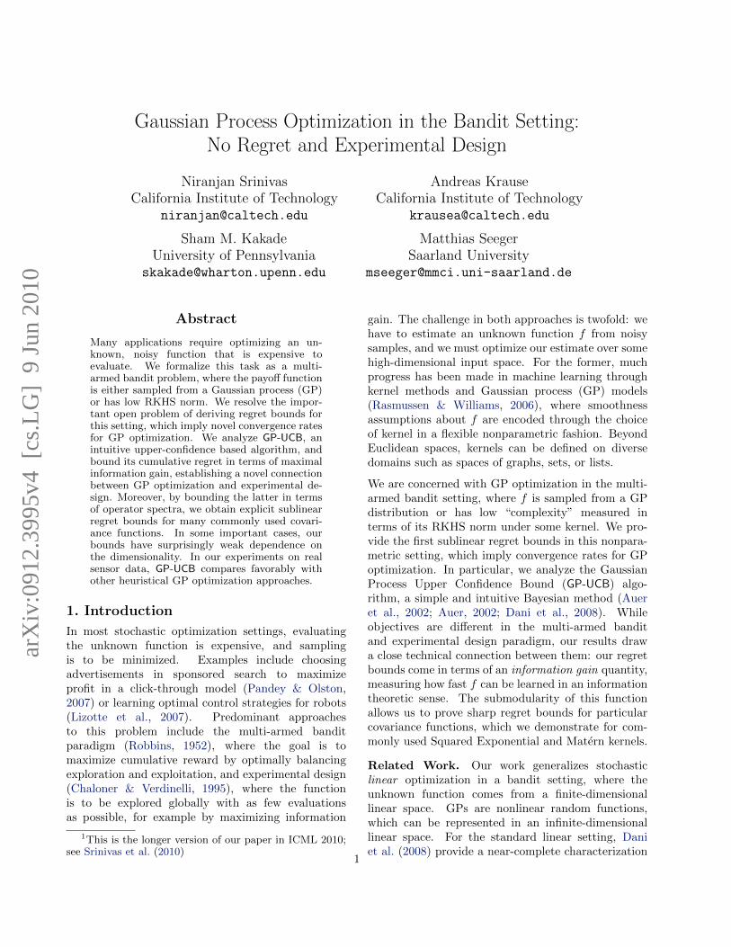
Therefore, if for some T∗ = o(T ) the first T∗ eigenval-ues carry most of the total mass nT , the informationgain will be small. The more rapidly the spectrumof KD decays, the slower the growth of γT . Figure 3illustrates this intuition.
5.2. Bounds for Common Kernels
In this section we bound γT for a range of commonlyused covariance functions: finite dimensional linear,Squared Exponential and Matern kernels. Togetherwith our results in Section 4, these imply sublinearregret bounds for GP-UCB in all cases.

5 10 15 200
5
10
15
Eigenvalue rank
Eig
enva
lue
Independent
Matern (ν = 2.5)
Squared exponential
Linear (d=4)
10 20 30 40 500
50
100
150
200
250
T
Bou
nd o
n γ T
Linear (d=4)
Independent
Matern
Squaredexponential
Figure 3. Spectral decay (left) and information gain bound (right) for independent (diagonal), linear, squared exponentialand Matern kernels (ν = 2.5.) with equal trace.
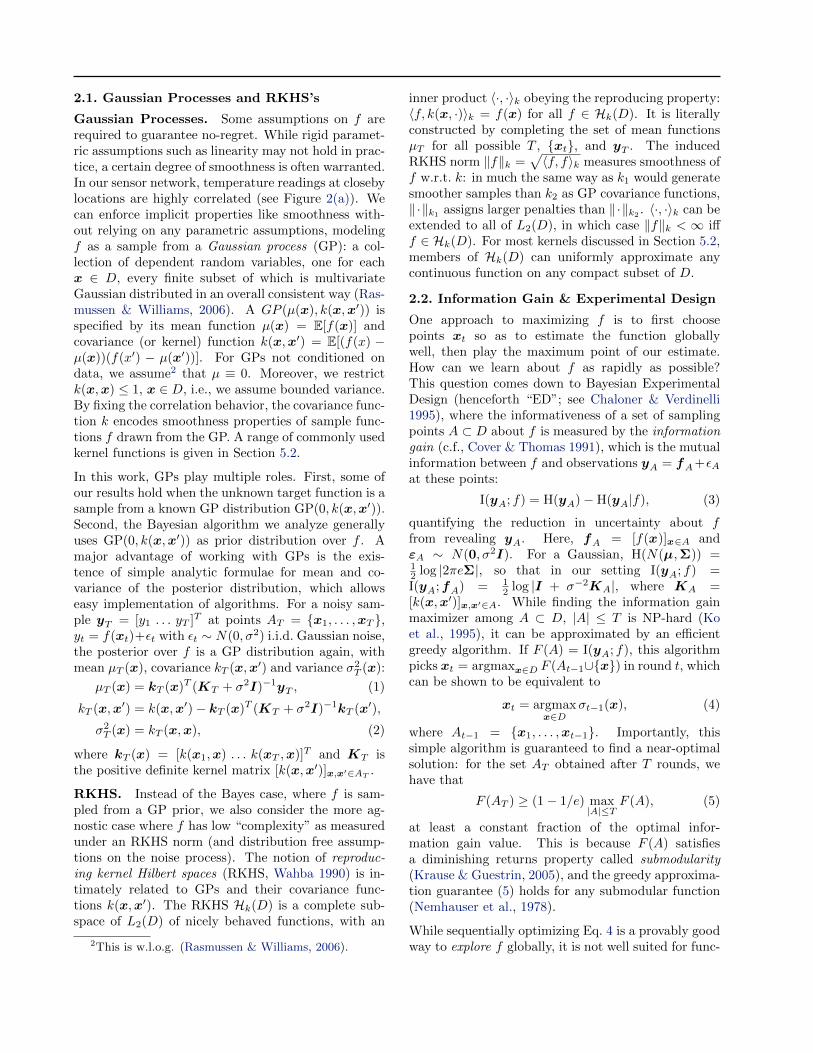
Finite dimensional linear kernels have the formk(x,x′) = xTx′. GPs with this kernel correspond torandom linear functions f(x) = wTx, w ∼ N(0, I).
The Squared Exponential kernel is k(x,x′) =exp(−(2l2)−1‖x − x′‖2), l a lengthscale parameter.Sample functions are differentiable to any orderalmost surely (Rasmussen & Williams, 2006).
The Matern kernel is given by k(x,x′) =(21−ν/Γ(ν))rνBν(r), r = (
√2ν/l)‖x − x′‖, where ν
controls the smoothness of sample paths (the smaller,the rougher) and Bν is a modified Bessel function.Note that as ν → ∞, appropriately rescaled Maternkernels converge to the Squared Exponential kernel.
Figure 4 shows random functions drawn from GP dis-tributions with the above kernels.
Theorem 5 Let D ⊂ Rd be compact and convex, d ∈N. Assume the kernel function satisfies k(x,x′) ≤ 1.
1. Finite spectrum. For the d-dimensional Bayesianlinear regression case: γT = O
(d log T
).
2. Exponential spectral decay. For the SquaredExponential kernel: γT = O
((log T )d+1
).
3. Power law spectral decay. For Matern kernelswith ν > 1: γT = O
(T d(d+1)/(2ν+d(d+1))(log T )
).
A proof of Theorem 5 is given in the Appendix, , weonly sketch the idea here. γT is bounded by Theo-rem 4 in terms the eigendecay of the kernel matrixKD. If D is infinite or very large, we can use theoperator spectrum of k(x,x′), which likewise decaysrapidly. For the kernels of interest here, asymptoticexpressions for the operator eigenvalues are givenin Seeger et al. (2008), who derived bounds on theinformation gain for fixed and random designs (incontrast to the worst-case information gain consideredhere, which is substantially more challenging tobound). The main challenge in the proof is to ensure
the existence of discretizations DT ⊂ D, dense in thelimit, for which tail sums B(T∗)/nT in Theorem 4 areclose to corresponding operator spectra tail sums.
Together with Theorems 2 and 3, this result guaran-tees sublinear regret of GP-UCB for any dimension(see Figure 1). For the Squared Exponential kernel,the dimension d appears as exponent of log T only, so
that the regret grows at most as O∗(√T (log T )
d+12 )
– the high degree of smoothness of the sample pathseffectively combats the curse of dimensionality.
6. Experiments
We compare GP-UCB with heuristics such as theExpected Improvement (EI) and Most ProbableImprovement (MPI), and with naive methods whichchoose points of maximum mean or variance only,both on synthetic and real sensor network data.
For synthetic data, we sample random functions from asquared exponential kernel with lengthscale parameter0.2. The sampling noise variance σ2 was set to 0.025 or5% of the signal variance. Our decision set D = [0, 1]is uniformly discretized into 1000 points. We runeach algorithm for T = 1000 iterations with δ = 0.1,averaging over 30 trials (samples from the kernel).While the choice of βt as recommended by Theorem 1leads to competitive performance of GP-UCB, wefind (using cross-validation) that the algorithm isimproved by scaling βt down by a factor 5. Note thatwe did not optimize constants in our regret bounds.
Next, we use temperature data collected from 46 sen-sors deployed at Intel Research Berkeley over 5 days at1 minute intervals, pertaining to the example in Sec-tion 2. We take the first two-thirds of the data set tocompute the empirical covariance of the sensor read-ings, and use it as the kernel matrix. The functions ffor optimization consist of one set of observations fromall the sensors taken from the remaining third of the

0 0.2 0.4 0.6 0.8 1−4
−2
0
2
4
6
(a) Bayesian Linear Regression
0 0.2 0.4 0.6 0.8 1−2
−1
0
1
2
(b) Squared Exponential
0 0.2 0.4 0.6 0.8 1−2
−1
0
1
2
(c) Matern
Figure 4. Sample functions drawn from a GP with linear, squared exponential and Matern kernels (ν = 2.5.)
0 20 40 60 80 1000
0.2
0.4
0.6
0.8
1
Iterations
Mea
n A
vera
ge R
egre
t
Var only
Mean only
MPI
EI
UCB
(a) Squared exponential
0 10 20 30 400
1
2
3
4
5
Iterations
Mea
n A
vera
ge R
egre
t
Var only
Mean onlyMPI
EIUCB
(b) Temperature data
0 100 200 3000
5
10
15
20
25
30
35
Iterations
Mea
n A
vera
ge R
egre
t
EI
MPI
Var onlyMean only
UCB
(c) Traffic data
Figure 5. Comparison of performance: GP-UCB and various heuristics on synthetic (a), and sensor network data (b, c).
data set, and the results (for T = 46, σ2 = 0.5 or 5%noise, δ = 0.1) were averaged over 2000 possiblechoices of the objective function.
Lastly, we take data from traffic sensors deployed alongthe highway I-880 South in California. The goal was tofind the point of minimum speed in order to identifythe most congested portion of the highway; we usedtraffic speed data for all working days from 6 AM to11 AM for one month, from 357 sensors. We againuse the covariance matrix from two-thirds of the dataset as kernel matrix, and test on the other third. Theresults (for T = 357, σ2 = 4.78 or 5% noise, δ = 0.1)were averaged over 900 runs.
Figure 5 compares the mean average regret incurredby the different heuristics and the GP-UCB algorithmon synthetic and real data. For temperature data,the GP-UCB algorithm and EI heuristic clearlyoutperform the others, and do not exhibit significantdifference between each other. On synthetic and traf-fic data MPI does equally well. In summary, GP-UCBperforms at least on par with the existing approacheswhich are not equipped with regret bounds.
7. Conclusions
We prove the first sublinear regret bounds for GPoptimization with commonly used kernels (see Fig-ure 1), both for f sampled from a known GP and f oflow RKHS norm. We analyze GP-UCB, an intuitive,
Bayesian upper confidence bound based sampling rule.Our regret bounds crucially depend on the informationgain due to sampling, establishing a novel connectionbetween bandit optimization and experimental design.We bound the information gain in terms of the kernelspectrum, providing a general methodology for obtain-ing regret bounds with kernels of interest. Our exper-iments on real sensor network data indicate that GP-UCB performs at least on par with competing criteriafor GP optimization, for which no regret bounds areknown at present. Our results provide an interestingstep towards understanding exploration–exploitationtradeoffs with complex utility functions.
Acknowledgements
We thank Marcus Hutter for insightful comments onan earlier version of this paper. This research waspartially supported by ONR grant N00014-09-1-1044,NSF grant CNS-0932392, a gift from Microsoft Cor-poration and the Excellence Initiative of the Germanresearch foundation (DFG).
References
Abernethy, J., Hazan, E., and Rakhlin, A. An efficientalgorithm for linear bandit optimization, 2008. COLT.
Auer, P. Using confidence bounds for exploitation-exploration trade-offs. JMLR, 3:397–422, 2002.
Auer, P., Cesa-Bianchi, N., and Fischer, P. Finite-time

analysis of the multiarmed bandit problem. Mach.Learn., 47(2-3):235–256, 2002.
Brochu, E., Cora, M., and de Freitas, N. A tutorial onBayesian optimization of expensive cost functions, withapplication to active user modeling and hierarchical re-inforcement learning. In TR-2009-23, UBC, 2009.
Bubeck, S., Munos, R., Stoltz, G., and Szepesvari, C. On-line optimization in X-armed bandits. In NIPS, 2008.
Chaloner, K. and Verdinelli, I. Bayesian experimental de-sign: A review. Stat. Sci., 10(3):273–304, 1995.
Cover, T. M. and Thomas, J. A. Elements of InformationTheory. Wiley Interscience, 1991.
Dani, V., Hayes, T. P., and Kakade, S. The price of banditinformation for online optimization. In NIPS, 2007.
Dani, V., Hayes, T. P., and Kakade, S. M. Stochastic linearoptimization under bandit feedback. In COLT, 2008.
Dorard, L., Glowacka, D., and Shawe-Taylor, J. Gaussianprocess modelling of dependencies in multi-armed banditproblems. In Int. Symp. Op. Res., 2009.
Freedman, D. A. On tail probabilities for martingales. Ann.Prob., 3(1):100–118, 1975.
Ghosal, S. and Roy, A. Posterior consistency of Gaussianprocess prior for nonparametric binary regression. Ann.Stat., 34(5):2413–2429, 2006.
Grunewalder, S., Audibert, J-Y., Opper, M., and Shawe-Taylor, J. Regret bounds for gaussian process banditproblems. In AISTATS, 2010.
Huang, D., Allen, T. T., Notz, W. I., and Zeng, N. Globaloptimization of stochastic black-box systems via sequen-tial kriging meta-models. J Glob. Opt., 34:441–466,2006.
Jones, D. R., Schonlau, M., and Welch, W. J. Efficientglobal optimization of expensive black-box functions. JGlob. Opti., 13:455–492, 1998.
Kleinberg, R., Slivkins, A., and Upfal, E. Multi-armedbandits in metric spaces. In STOC, pp. 681–690, 2008.
Ko, C., Lee, J., and Queyranne, M. An exact algorithmfor maximum entropy sampling. Ops Res, 43(4):684–691,1995.
Kocsis, L. and Szepesvari, C. Bandit based monte-carloplanning. In ECML, 2006.
Krause, A. and Guestrin, C. Near-optimal nonmyopic valueof information in graphical models. In UAI, 2005.
Lizotte, D., Wang, T., Bowling, M., and Schuurmans, D.Automatic gait optimization with Gaussian process re-gression. In IJCAI, pp. 944–949, 2007.
McDiarmid, C. Concentration. In Probabilistiic Methodsfor Algorithmic Discrete Mathematics. Springer, 1998.
Mockus, J. Bayesian Approach to Global Optimization.Kluwer Academic Publishers, 1989.
Mockus, J., Tiesis, V., and Zilinskas, A. Toward GlobalOptimization, volume 2, chapter Bayesian Methods forSeeking the Extremum, pp. 117–128. 1978.
Nemhauser, G., Wolsey, L., and Fisher, M. An analysisof the approximations for maximizing submodular setfunctions. Math. Prog., 14:265–294, 1978.
Pandey, S. and Olston, C. Handling advertisements of un-known quality in search advertising. In NIPS. 2007.
Rasmussen, C. E. and Williams, C. K. I. Gaussian Pro-cesses for Machine Learning. MIT Press, 2006.
Robbins, H. Some aspects of the sequential design of ex-periments. Bul. Am. Math. Soc., 58:527–535, 1952.
Rusmevichientong, P. and Tsitsiklis, J. N. Linearly param-eterized bandits. abs/0812.3465, 2008.
Seeger, M. W., Kakade, S. M., and Foster, D. P. Infor-mation consistency of nonparametric Gaussian processmethods. IEEE Tr. Inf. Theo., 54(5):2376–2382, 2008.
Shawe-Taylor, J., Williams, C., Cristianini, N., and Kan-dola, J. On the eigenspectrum of the Gram matrix andthe generalization error of kernel-PCA. IEEE Trans. Inf.Theo., 51(7):2510–2522, 2005.
Srinivas, N., Krause, A., Kakade, S., and Seeger, M. Gaus-sian process optimization in the bandit setting: No re-gret and experimental design. In ICML, 2010.
Stein, M. Interpolation of Spatial Data: Some Theory forKriging. Springer, 1999.
Vazquez, E. and Bect, J. Convergence properties of theexpected improvement algorithm, 2007.
Wahba, G. Spline Models for Observational Data. SIAM,1990.
A. Regret Bounds for Target FunctionSampled from GP
In this section, we provide details for the proofs ofTheorem 1 and Theorem 2. In both cases, the strategy
is to show that |f(x)−µt−1(x)| ≤ β1/2t σt−1(x) for all
t ∈ N and all x ∈ D, or in the infinite case, all x ina discretization of D which becomes dense as t getslarge.
A.1. Finite Decision Set
We begin with the finite case, |D| <∞.
Lemma 5.1 Pick δ ∈ (0, 1) and set βt =2 log(|D|πt/δ), where
∑t≥1 π
−1t = 1, πt > 0. Then,
|f(x)− µt−1(x)| ≤ β1/2t σt−1(x) ∀x ∈ D ∀t ≥ 1
holds with probability ≥ 1− δ.

Proof Fix t ≥ 1 and x ∈ D. Conditioned on yt−1 =(y1, . . . , yt−1), x1, . . . ,xt−1 are deterministic, andf(x) ∼ N(µt−1(x), σ2
t−1(x)). Now, if r ∼ N(0, 1),then
Prr > c = e−c2/2(2π)−1/2
∫e−(r−c)
2/2−c(r−c) dr
≤ e−c2/2 Prr > 0 = (1/2)e−c
2/2
for c > 0, since e−c(r−c) ≤ 1 for r ≥ c. Therefore,
Pr|f(x) − µt−1(x)| > β1/2t σt−1(x) ≤ e−βt/2, using
r = (f(x)−µt−1(x))/σt−1(x) and c = β1/2t . Applying
the union bound,
|f(x)− µt−1(x)| ≤ β1/2t σt−1(x) ∀x ∈ D
holds with probability ≥ 1 − |D|e−βt/2. Choosing|D|e−βt/2 = δ/πt and using the union bound fort ∈ N, the statement holds. For example, we can useπt = π2t2/6.
Lemma 5.2 Fix t ≥ 1. If |f(x) − µt−1(x)| ≤β1/2t σt−1(x) for all x ∈ D, then the regret rt is
bounded by 2β1/2t σt−1(xt).
Proof By definition of xt: µt−1(xt)+β1/2t σt−1(xt) ≥
µt−1(x∗) + β1/2t σt−1(x∗) ≥ f(x∗). Therefore,
rt = f(x∗)− f(xt) ≤ β1/2t σt−1(xt) + µt−1(xt)− f(xt)
≤ 2β1/2t σt−1(xt).
Lemma 5.3 The information gain for the points se-lected can be expressed in terms of the predictive vari-ances. If fT = (f(xt)) ∈ RT :
I(yT ;fT ) =1
2
∑T
t=1log(1 + σ−2σ2
t−1(xt)).
Proof Recall that I(yT ;fT ) = H(yT ) −(1/2) log |2πeσ2I|. Now, H(yT ) = H(yT−1) +H(yT |yT−1) = H(yT−1) + log(2πe(σ2 + σ2
t−1(xT )))/2.Here, we use that x1, . . . ,xT are deterministic con-ditioned on yT−1, and that the conditional varianceσ2T−1(xT ) does not depend on yT−1. The result fol-
lows by induction.
Lemma 5.4 Pick δ ∈ (0, 1) and let βt be defined as inLemma 5.1. Then, the following holds with probability≥ 1− δ:∑T
t=1r2t ≤ βTC1I(yT ;fT ) ≤ C1βT γT ∀T ≥ 1,
where C1 := 8/ log(1 + σ−2) ≥ 8σ2.
Proof By Lemma 5.1 and Lemma 5.2, we have thatr2t ≤ 4βtσ
2t−1(xt) ∀t ≥ 1 with probability ≥ 1 − δ.
Now, βt is nondecreasing, so that
4βtσ2t−1(xt) ≤ 4βTσ
2(σ−2σ2t−1(xt))
≤ 4βTσ2C2 log(1 + σ−2σ2
t−1(xt))
with C2 = σ−2/ log(1 + σ−2) ≥ 1, sinces2 ≤ C2 log(1 + s2) for s ∈ [0, σ−2], andσ−2σ2
t−1(xt) ≤ σ−2k(xt,xt) ≤ σ−2. Noting thatC1 = 8σ2C2, the result follows by plugging in therepresentation of Lemma 5.3.
Finally, Theorem 1 is a simple consequence ofLemma 5.4, since R2
T ≤ T∑Tt=1 r
2t by the Cauchy-
Schwarz inequality.
A.2. General Decision Set
Theorem 2 extends the statement of Theorem 1 tothe general case of D ⊂ Rd compact. We cannotexpect this generalization to work without any as-sumptions on the kernel k(x,x′). For example, ifk(x,x′) = e−‖x−x
′‖ (Ornstein-Uhlenbeck), while sam-ple paths f are a.s. continuous, they are still very er-ratic: f is a.s. nondifferentiable almost everywhere,and the process comes with independent increments, astationary variant of Brownian motion. The additionalassumption on k in Theorem 2 is rather mild and issatisfied by several common kernels, as discussed inSection 4.
Recall that the finite case proof is based on Lemma 5.1paving the way for Lemma 5.2. However, Lemma 5.1does not hold for infinite D. First, let us observe thatwe have confidence on all decisions actually chosen.
Lemma 5.5 Pick δ ∈ (0, 1) and set βt = 2 log(πt/δ),where
∑t≥1 π
−1t = 1, πt > 0. Then,
|f(xt)− µt−1(xt)| ≤ β1/2t σt−1(xt) ∀t ≥ 1
holds with probability ≥ 1− δ.
Proof Fix t ≥ 1 and x ∈ D. Conditioned onyt−1 = (y1, . . . , yt−1), x1, . . . ,xt−1 are determin-istic, and f(x) ∼ N(µt−1(x), σ2
t−1(x)). As before,
Pr|f(xt) − µt−1(xt)| > β1/2t σt−1(xt) ≤ e−βt/2.
Since e−βt/2 = δ/πt and using the union bound fort ∈ N, the statement holds.
Purely for the sake of analysis, we use a set of dis-cretizations Dt ⊂ D, where Dt will be used at time

t in the analysis. Essentially, we use this to obtain avalid confidence interval on x∗. The following lemmaprovides a confidence bound for these subsets.
Lemma 5.6 Pick δ ∈ (0, 1) and set βt =2 log(|Dt|πt/δ), where
∑t≥1 π
−1t = 1, πt > 0. Then,
|f(x)− µt−1(x)| ≤ β1/2t σt−1(x) ∀x ∈ Dt, ∀t ≥ 1
holds with probability ≥ 1− δ.
Proof The proof is identical to that in Lemma 5.1,except now we use Dt at each timestep.
Now by assumption and the union bound, we have that
Pr ∀j, ∀x ∈ D, |∂f/(∂xj)| < L ≥ 1− dae−L2/b2 .
which implies that, with probability greater than 1 −dae−L
2/b2 , we have that
∀x ∈ D, |f(x)− f(x′)| ≤ L‖x− x′‖1 . (9)
This allows us to obtain confidence on x? as follows.
Now let us choose a discretization Dt of size (τt)d so
that for all x ∈ Dt
‖x − [x]t‖1 ≤ rd/τt
where [x]t denotes the closest point in Dt to x. A suf-ficient discretization has each coordinate with τt uni-formly spaced points.
Lemma 5.7 Pick δ ∈ (0, 1) and set βt =2 log(2πt/δ) + 4d log(dtbr
√log(2da/δ)), where∑
t≥1 π−1t = 1, πt > 0. Let τt = dt2br
√log(2da/δ)
Let [x∗]t denotes the closest point in Dt to x∗. Hence,Then,
|f(x∗)− µt−1([x∗]t)| ≤ β1/2t σt−1([x∗]t) +
1
t2∀t ≥ 1
holds with probability ≥ 1− δ.
Proof Using (9), we have that with probabilitygreater than 1− δ/2,
∀x ∈ D, |f(x)− f(x′)| ≤ b√
log(2da/δ)‖x− x′‖1 .
Hence,
∀x ∈ Dt, |f(x)− f([x]t)| ≤ rdb√
log(2da/δ)/τt .
Now by choosing τt = dt2br√
log(2da/δ), we have that
∀x ∈ Dt, |f(x)− f([x]t)| ≤1
t2
This implies that |Dt| = (dt2br√
log(2da/δ))d. Usingδ/2 in Lemma 5.6, we can apply the confidence boundto [x∗]t (as this lives in Dt) to obtain the result.
Now we are able to bound the regret.
Lemma 5.8 Pick δ ∈ (0, 1) and set βt =2 log(4πt/δ) + 4d log(dtbr
√log(4da/δ)), where∑
t≥1 π−1t = 1, πt > 0. Then, with probability greater
than 1 − δ, for all t ∈ N, the regret is bounded asfollows:
rt ≤ 2β1/2t σt−1(xt) +
1
t2.
Proof We use δ/2 in both Lemma 5.5 and Lemma 5.7,so that these events hold with probability greaterthan 1 − δ. Note that the specification of βt in theabove lemma is greater than the specification used inLemma 5.5 (with δ/2), so this choice is valid.
By definition of xt: µt−1(xt) + β1/2t σt−1(xt) ≥
µt−1([x∗]t)+β1/2t σt−1([x∗]t). Also, by Lemma 5.7, we
have that µt−1([x∗]t)+β1/2t σt−1([x∗]t)+1/t2 ≥ f(x∗),
which implies µt−1(xt)+β1/2t σt−1(xt) ≥ f(x∗)−1/t2.
Therefore,
rt = f(x∗)− f(xt)
≤ β1/2t σt−1(xt) + 1/t2 + µt−1(xt)− f(xt)
≤ 2β1/2t σt−1(xt) + 1/t2 .
which completes the proof.
Now we are ready to complete the proof of Theorem 2.As shown in the proof of Lemma 5.4, we have that withprobability greater than 1− δ,∑T
t=14βtσ
2t−1(xt) ≤ C1βT γT ∀T ≥ 1,
so that by Cauchy-Schwarz:∑T
t=12β
1/2t σt−1(xt) ≤
√C1TβT γT ∀T ≥ 1,
Hence,∑T
t=1rt ≤
√C1TβT γT + π2/6 ∀T ≥ 1,
(since∑
1/t2 = π2/6). Theorem 2 now follows.
Finally, we now discuss the additional assumption onk in Theorem 2. For samples f of the GP, considerpartial derivatives ∂f/(∂xj) of this sample path forj = 1, . . . , d. Theorem 5 of Ghosal & Roy (2006)

states that if derivatives up to fourth order existsfor (x,x′) 7→ k(x,x′), then f is almost surely con-tinuously differentiable, with ∂f/(∂xj) distributed asGaussian processes again. Moreover, there are con-stants a, bj > 0 such that
Pr
supx∈D|∂f/(∂xj)| > L
≤ ae−bjL
2
. (10)
Picking L = [log(da2/δ)/minj bj ]1/2, we have that
ae−bjL2 ≤ δ/(2d) for all j = 1, . . . , d, so that for
K1 = d1/2L, by the mean value theorem, we havePr|f(x)−f(x′)| ≤ K1‖x−x′‖ ∀ x,x′ ∈ D ≥ 1−δ/2.
Also, note that K1 = O((log δ−1)1/2).
This statement is about the joint distribution of f(·)and its partial derivatives w.r.t. each component. Fora certain event in this sample space, all ∂f/(∂xj) ex-ist, are continuous, and the complement of (10) holdsfor all j. Theorem 5 of Ghosal & Roy (2006), togetherwith the union bound, implies that this event has prob-ability ≥ 1− δ/2. Derivatives up to fourth order existfor the Gaussian covariance function, and for Maternkernels with ν > 2 (Stein, 1999).
B. Regret Bound for Target Functionin RKHS
In this section, we detail a proof of Theorem 3. Recallthat in this setting, we do not know the generator ofthe target function f , but only a bound on its RKHSnorm ‖f‖k.
Recall the posterior mean function µT (·) and posteriorcovariance function kT (·, ·) from Section 2, conditionedon data (xt, yt), t = 1, . . . , T . It is easy to see that theRKHS norm corresponding to kT is given by
‖f‖2kT = ‖f‖2k + σ−2∑T
t=1f(xt)
2.
This implies that Hk(D) = HkT (D) for any T , whilethe RKHS inner products are different: ‖f‖kT ≥ ‖f‖k.Since 〈f(·), kT (·,x)〉kT = f(x) for any f ∈ HkT (D) bythe reproducing property, then
|µt(x)− f(x)| ≤ kT (x,x)1/2‖µt − f‖kT= σT (x)‖µt − f‖kT
(11)
by the Cauchy-Schwarz inequality.
Compared to our other results, Theorem 3 is an agnos-tic statement, in that the assumptions the BayesianUCB algorithm bases its predictions on differ fromhow f and data yt are generated. First, f is notdrawn from a GP, but can be an arbitrary function
from Hk(D). Second, while the UCB method assumesthat the noise εt = yt − f(xt) is drawn independentlyfrom N(0, σ2), the true sequence of noise variables εtcan be a uniformly bounded martingale difference se-quence: εt ≤ σ for all t ∈ N. All we have to do in orderto lift the proof of Theorem 1 to the agnostic settingis to establish an analogue to Lemma 5.1, by way ofthe following concentration result.
Theorem 6 Let δ ∈ (0, 1). Assume the noise vari-ables εt are uniformly bounded by σ. Define:
βt = 2‖f‖2k + 300γt ln3(t/δ),
Then
Pr∀T, ∀x ∈ D, |µT (x)− f(x)| ≤ β1/2
T+1σT (x)≥ 1−δ.
B.1. Concentration of Martingales
In our analysis, we use the following Bernstein-typeconcentration inequality for martingale differences,due to Freedman (1975) (see also Theorem 3.15 of Mc-Diarmid 1998).
Theorem 7 (Freedman) Suppose X1, . . . , XT is amartingale difference sequence, and b is an uniformupper bound on the steps Xi. Let V denote the sum ofconditional variances,
V =∑n
i=1Var (Xi |X1, . . . , Xi−1).
Then, for every a, v > 0,
Pr∑
Xi ≥ a and V ≤ v≤ exp
(−a2
2v + 2ab/3
).
B.2. Proof of Theorem 6
We will show that:
Pr∀T, ‖µT − f‖2kT ≤ βT+1
≥ 1− δ.
Theorem 6 then follows from (11). Recall that εt =yt − f(xt). We will analyze the quantity ZT =‖µT − f‖2kT , measuring the error of µT as approxi-mation to f under the RKHS norm of HkT (D). Thefollowing lemma provides the connection with the in-formation gain. This lemma is important since ourconcentration argument is an inductive argument —roughly speaking, we condition on getting concentra-tion in the past, in order to achieve good concentrationin the future.
Lemma 7.1 We have that∑T
t=1minσ−2σ2
t−1(xt), α ≤2α
log(1 + α)γT , α > 0.

Proof We have that minr, α ≤ (α/ log(1 +α)) log(1+r). The statement follows from Lemma 5.3.
The next lemma bounds the growth of ZT . It is for-mulated in terms of normalized quantities: εt = εt/σ,
f = f/σ, µt = µt/σ, σt = σt/σ. Also, to ease nota-tion, we will use µt−1, σt−1 as shorthand for µt−1(xt),σt−1(xt).
Lemma 7.2 For all T ∈ N,
ZT ≤ ‖f‖2k + 2∑T
t=1εtµt−1 − f(xt)
1 + σ2t−1
+∑T
t=1ε2t
σ2t−1
1 + σ2t−1
.
Proof If αt = (Kt + σ2I)−1yt, then µt(x) =αTt kt(x). Then, 〈µT , f〉k = fTTαT , ‖µT ‖2k =yTTαT − σ2‖αT ‖2. Moreover, for t ≤ T , µT (xt) =
δTt KT (KT + σ2I)−1yT = yt − σ2αt. Since ZT =‖µT −f‖k+σ−2
∑t≤T (µT (xt)−f(xt))
2, we have that
ZT = ‖f‖2k − 2fTTαT + yTTαT − σ2‖αT ‖2
+ σ−2∑T
t=1(εt − σ2αt)
2 = ‖f‖2k− yTT (KT + σ2I)−1yT + σ−2‖εT ‖2.
Now, −yTT (KT +σ2I)−1yT.= 2 logP (yT ), where “
.=”
means that we drop determinant terms, thus con-centrate on quadratic functions. Since logP (yT ) =∑t logP (yt|y<t) =
∑t logN(yt|µt−1(xt), σ
2t−1(xt) +
σ2), we have that
− yTT (KT + σ2I)−1yT = −∑
t
(yt − µt−1)2
σ2 + σ2t−1
= 2∑
tεtµt−1 − f(xt)
σ2 + σ2t−1
−∑
t
ε2t σ2t−1
σ2 + σ2t−1−R
with R =∑t(µt−1 − f(xt))
2/(σ2 + σ2t−1) ≥ 0.
Dropping −R and changing to normalized quantitiesconcludes the proof.
We now define a useful martingale difference sequence.First, it is convenient to define an “escape event” ETas:
ET = IZt ≤ βt+1 for all t ≤ Twhere I· is the indicator function. Define the randomvariables Mt by
Mt = 2εtEt−1µt−1 − f(xt)
1 + σ2t−1
.
Now, since εt is a martingale difference sequence withrespect to the histories H<t and Mt/εt is determinis-tic given H<t, Mt is a martingale difference sequenceas well. Next, we show that with high probability,the associated martingale
∑Tt=1Mt does not grow too
large.
Lemma 7.3 Given δ ∈ (0, 1) and βt as defined in inTheorem 6, we have that
Pr
∀T,
T∑t=1
Mt ≤ βT+1/2
≥ 1− δ,
The proof is given below in Section B.3. Equippedwith this lemma, we can prove Theorem 6.
Proof [of Theorem 6] It suffices to show that the high-probability event described in Lemma 7.3 is containedin the support of ET for every T . We prove the latterby induction on T .
By Lemma 7.2 and the definition of β1, we know thatZ0 ≤ ‖f‖k ≤ β1. Hence E0 = 1 always. Now supposethe high-probability event of Lemma 7.3 holds, in par-ticular
∑Tt=1Mt ≤ βT+1/2. For the inductive hypoth-
esis, assume ET−1 = 1. Using this and Lemma 7.2:
ZT ≤ ‖f‖2k + 2
T∑t=1
εt(µt−1 − f(xt))
1 + σ2t−1
+
T∑t=1
ε2t σ2t−1
1 + σ2t−1
= ‖f‖2k +
T∑t=1
Mt +
T∑t=1
ε2tσ2t−1
1 + σ2t−1
≤ ‖f‖2k + βT+1/2 +
T∑t=1
minσ2t−1, 1
≤ ‖f‖2k + βT+1/2 + (2/ log 2)γT ≤ βT+1.
The equality in the second step uses the inductivehypothesis. Thus we have shown ET = 1, completingthe induction.
B.3. Concentration
What remains to be shown is Lemma 7.3. While thestep sizes |Mt| are uniformly bounded, a standard ap-plication of the Hoeffding-Azuma inequality leads toa bound of T 3/4, too large for our purpose. We usethe more specific Theorem 7 instead, which requiresto control the conditional variances rather than themarginal variances which can be much larger.
Proof [of Lemma 7.3] Let us first obtain upper bounds
on the step sizes of our martingale.
|Mt| = 2|εt|Et−1|µt−1 − f(xt)|
1 + σ2t−1
≤ 2|εt|Et−1β1/2t σt−1
1 + σ2t−1
≤ 2|εt|Et−1β1/2t minσt−1, 1/2, (12)
where the first inequality follows from the definitionof Et. Moreover, r/(1 + r2) ≤ minr, 1/2 for r ≥ 0.
Therefore, |Mt| ≤ β1/2T , since |εt| ≤ 1 and βt in nonde-
creasing. Next, we bound the sum of the conditionalvariances of the martingale:
VT :=∑T
t=1Var (Mt |M1 . . .Mt−1)
≤∑T
t=14|εt|2Et−1βt minσ2
t−1, 1/4
≤ 4βT∑T
t=1Et−1 minσ2
t−1, 1/4 |εt| ≤ 1
≤ 9βT γT .
In the last line, we used Lemma 7.1 with α = 1/4, not-ing that 8α/ log(1 +α) ≤ 9. Since we have establishedthat the sum of conditional variances, VT , is alwaysbounded by 9βT γT , we can apply Theorem 7 with pa-
rameters a = βT+1/2, b = β1/2T+1 and v = 9βT γT to
get
Pr
∑T
t=1Mt ≥ βT+1/2
= Pr
∑T
t=1Mt ≥ βT+1/2 and VT ≤ 9βT γT
≤ exp
(−(βT+1/2)2
2(9βT γT ) + 23 (βT+1/2)β
1/2T+1
)
= exp
(−βT+1
72γT + 43β
1/2T+1
)
≤ max
exp
(−βT+1
144γT
), exp
(−3β
1/2T+1
8
).
Note that our choice of βT+1 satisfies:
max
144γT log(T 2/δ),((8/3) log(T 2/δ)
)2 ≤ βT+1.
Therefore, the previous probability is bounded byδ/T 2, whereas the last inequality follows from the def-inition of βT+1. With a final application of the union
bound:
Pr
∑T
t=1Mt ≥ βT+1/2 for some T
≤∑
T≥1Pr
∑T
t=1Mt ≥ βT+1/2
≤∑
T≥2δ/T 2 ≤ δ(π2/6− 1) ≤ δ,
completing the proof of Lemma 7.3.
C. Bounds on Information Gain
In this section, we show how to bound γT , the max-imum information gain after T rounds, for compactD ⊂ Rd (assumptions of Theorem 2) and several com-monly used covariance functions. In this section, weassume4 that k(x,x) = 1 for all x ∈ D.
The plan of attack is as follows. First, we note that theargument of γT , I(yA;fA) is a submodular function,so γT can be bounded by the value obtained by greedymaximization. Next, we use a discretization DT ⊂ Dwith nT = |DT | = T τ with nearest neighbour distanceo(1), consider the kernel matrix KDT
∈ RnT×nT , andbound γT by an expression involving the eigenvaluesλt of this matrix, which is done by a further re-laxation of the greedy procedure. Finally, we boundthis empirical expression in terms of the kernel opera-tor eigenvalues of k w.r.t. the uniform distribution onD. Asymptotic expressions for the latter are reviewedin Seeger et al. (2008), which we plug in to obtainour results. A key step in this argument is to ensurethe existence of a discretization DT , for which tailsof the empirical spectrum can be bounded by tails ofthe process spectrum. We will invoke the probabilisticmethod for that.
C.1. Greedy Maximization and Discretization
In this section, we fix T ∈ N and assume the existenceof a discretization DT ⊂ D, nT = |DT | on the orderof T τ , such that:
∀x ∈ D ∃[x]T ∈ DT : ‖x− [x]T ‖ = O(T−τ/d). (13)
We come back to the choice of DT below. We restrictthe information gain to subsets A ⊂ DT :
γT = maxA⊂DT ,|A|=T
I(yA;fA).
Of course, γT ≤ γT , but we can bound the slack.
4 Without loss in generality. We use this assumptionbelow to ensure that n−1
T trKDT =∫k(x,x) dx. If k(x,x)
is not constant, this is approximately true by the law oflarge numbers, and our result below remains valid.

Lemma 7.4 Under the assumptions of Theorem 2,the information gain FT (xt) = (1/2) log |I +σ−2Kxt| is uniformly Lipschitz-continuous in eachcomponent xt ∈ D.
Proof The assumptions of Theorem 2 imply thatthe kernel K(x,x′) is continuously differentiable.The result follows from the fact that FT (xt) iscontinuously differentiable in the kernel matrixKxt.
Lemma 7.5 Let DT be a discretization of D such that(13) holds. Under the assumptions of Theorem 2, wehave that
0 ≤ γT − γT = O(T 1−τ/d).
Proof Fix T ∈ N, and let A = x1, . . . ,xT be amaximizer for γT . Consider neighbours [xt]T ∈ DT
according to (13), [A]T = [xt]T . Then,
0 ≤ γT−γT ≤ γT−I(y[A]T ;f [A]T ) = FT (A)−FT ([A]T ),
where FT (xt) = (1/2) log |I + σ−2Kxt|. ByLemma 7.4, FT is uniformly Lipschitz-continuousin each component, so that |γT − I(y[A]T ;f [A]T )| =
O(T maxt ‖xt − [xt]T ‖) = O(T 1−τ/d) by (13) and themean value theorem.
We concentrate on γT in the sequel. Let KDT=
[k(x,x′)]x,x′∈DTbe the kernel matrix over the en-
tire DT , and KDT= U ΛUT its eigendecomposi-
tion, with λ1 ≥ λ2 ≥ · · · ≥ 0 and U = [u1 u2 . . . ]
orthonormal. Here, if T > nT , define λt = 0 fort = nT + 1, . . . , T . Information gain maximizationover a finite DT can be described in terms of a sim-ple linear-Gaussian model over the unknown f ∈ RnT ,with prior P (f ) = N(0,KDT
) and likelihood poten-tials P (yt|f ) = N(vTt f , σ
2) with unit-norm features,‖vt‖ = 1. With the following lemma, we upper-boundγT by way of two relaxations.
Lemma 7.6 For any T ≥ 1, we have that
γT ≤1/2
1− e−1max
m1,...,mT
∑T
t=1log(1 + σ−2mtλt),
subject to mt ∈ N,∑tmT = T , where λ1 ≥ λ2 ≥ . . .
is the spectrum of the kernel matrix KDT. Here, if
T > nT , then mt = 0 for t > nT .
Proof As shown by Krause & Guestrin (2005),the function F (A) = I(yA;f ) is submodular. In
the particular case considered here, this can be seenas follows: F (A) = H(yA) − H(yA | f ), wherethe entropy H(yA) is a (not-necessarily monotonic)submodular function in A, and since the noise isconditionally independent given f , H(yA | f ) isan additive (modular) function in A. Subtractinga modular function preserves submodularity, thusF (A) is submodular. Furthermore, the informationgain is monotonic in A (i.e., F (A) ≤ F (B) wheneverA ⊆ B) (Cover & Thomas, 1991). Thus, we canapply the result of Nemhauser et al. (1978)5 whichguarantees that γT is upper-bounded by 1/(1 − 1/e)times the value the greedy maximization algorithmattains. The latter chooses features of the formvt = δxt = [Ix=xt] in each round, xt ∈ DT . Weupper-bound the greedy maximum once more byrelaxing these constraints to ‖vt‖ = 1 only. In theremainder of the proof, we concentrate on this relaxedgreedy procedure. Suppose that up to round t, it chosev1, . . . ,vt−1. The posterior P (f |yt−1) has inverse
covariance matrix Σ−1t−1 = K−1DT+ σ−2V t−1V
Tt−1,
V t−1 = [v1 . . . vt−1], and the greedy procedureselects v so to maximize the variance vTΣt−1v : theeigenvector corresponding to Σt−1’s largest eigenvalue(by the Rayleigh-Ritz theorem). Since Σ0 = KDT
,then v1 = u1. Moreover, if all vt′ , t
′ < t, havebeen chosen among U ’s columns, then by the inversecovariance expression just given, KDT
and Σt−1 havethe same eigenvectors, so that vt is a column of U aswell. For example, if vt = uj , then comparing Σt−1and Σt, all eigenvalues other than the j-th remainthe same, while the latter is shrunk. Therefore,after T rounds of the relaxed greedy procedure:vt ∈ u1, . . . ,uminT,nT , t = 1, . . . , T : at most theleading T eigenvectors of KDT
can have been selected(possibly multiple times). If mt denotes the numberthat the t-th column of U has been selected, we ob-tain the theorem statement by a final bounding step.
C.2. From Empirical to Process Eigenvalues
The final step will be to relate the empirical spec-trum λt to the kernel operator spectrum. Since
log(1 + σ−2mtλt) ≤ σ−2mtλt in Theorem 7.6, we willmainly be interested in relating the tail sums of thespectra. Let µ(x) = V(D)−1Ix∈D be the uniformdistribution on D, V(D) =
∫x∈D dx, and assume that
k is continuous. Note that∫k(x,x)µ(x) dx = 1 by
our assumption k(x,x) = 1, so that k is Hilbert-
5While the result of Nemhauser et al. (1978) is statedin terms of finite sets, it extends to infinite sets as long asthe greedy selection can be implemented efficiently.

Schmidt on L2(µ). Then, Mercer’s theorem (Wahba,1990) states that the corresponding kernel operatorhas a discrete eigenspectrum (λs, φs(·)), and
k(x,x′) =∑
s≥1λsφs(x)φs(x
′),
where λ1 ≥ λ2 ≥ · · · ≥ 0, and Eµ[φs(x)φt(x)] =δs,t. Moreover,
∑s≥1 λ
2s < ∞, and the expan-
sion of k converges absolutely and uniformly on D ×D. Note that
∑s≥1 λs =
∑s≥1 λs Eµ[φs(x)2] =∫
K(x,x)µ(x) dx = 1. In order to proceed from The-orem 7.6, we have to pick a discretization DT for which(13) holds, and for which
∑t>T∗
λt is not much largerthan
∑t>T∗
λt. With the following lemma, we deter-mine sizes nT for which such discretizations exist.
Lemma 7.7 Fix T ∈ N, δ > 0 and ε > 0. Thereexists a discretization DT ⊂ D of size
nT = V(D)(ε/√d)−d[log(1/δ)+d log(
√d/ε)+logV(D)]
which fulfils the following requirements:
• ε-denseness: For any x ∈ D, there exists [x]T ∈DT such that ‖x − [x]T ‖ ≤ ε.
• If spec(KDT) = λ1 ≥ λ2 ≥ . . . , then for any
T∗ = 1, . . . , nT :
n−1T∑T∗
t=1λt ≥
∑T∗
t=1λt − δ.
Proof First, if we draw nT samples xj ∼ µ(x) in-dependently at random, then DT = xj is ε-densewith probability ≥ 1 − δ. Namely, cover D withN = V(D)(ε/
√d)−d hypercubes of sidelength ε/
√d,
within which the maximum Euclidean distance is ε.The probability of not hitting at least one cell is upper-bounded by N(1 − 1/N)nT . Since log(1 − 1/N) ≤−1/N , this is upper-bounded by δ if nT ≥ N log(N/δ).
Now, let S = n−1T∑T∗t=1 λt. Shawe-Taylor et al.
(2005) show that E[S] ≥∑T∗t=1 λt. If C is the
event DT is ε−dense , then Pr(C) ≥ 1 − δ. SinceS ≤ n−1T trKDT
= 1 in any case, we have that
E[S|C] ≥ E[S] − Pr(Cc) ≥∑T∗t=1 λt − δ. By the
probabilistic method, there must exist some DT forwhich C and the latter inequality holds.
The following lemma, the equivalent of Theorem 4 inthe context here, is a direct consequence of Lemma 7.6.
Lemma 7.8 Let DT be some discretization of D,
nT = |DT |. Then, for any T∗ = 1, . . . ,minT, nT :
γT ≤1/2
1− e−1max
r=1,...,T
(T∗ log(rnT /σ
2)
+ (T − r)σ−2∑nT
t=T∗+1λt
).
Proof We split the right hand side in Lemma 7.6at t = T∗. Let r =
∑t≤T∗ mt. For t ≤ T∗:
log(1 + mtλt/σ2) ≤ log(rnT /σ
2), since λt ≤ nT . For
t > T∗: log(1+mtλt/σ2) ≤ mtλt/σ
2 ≤ (T−r)λt/σ2.
The following theorem describes our “recipe” for ob-taining bounds on γT for a particular kernel k, giventhat tail bounds on Bk(T∗) =
∑s>T∗
λs are known.
Theorem 8 Suppose that D ⊂ Rd is compact, andk(x,x′) is a covariance function for which the ad-ditional assumption of Theorem 2 holds. Moreover,let Bk(T∗) =
∑s>T∗
λs, where λs is the operatorspectrum of k with respect to the uniform distributionover D. Pick τ > 0, and let nT = C4T
τ (log T ) withC4 = 2V(D)(2τ + 1). Then, the following bound holdstrue:
γT ≤1/2
1− e−1max
r=1,...,T
(T∗ log(rnT /σ
2)
+ C4σ−2(1− r/T )(log T )
(T τ+1Bk(T∗) + 1
))+O(T 1−τ/d)
for any T∗ ∈ 1, . . . , nT .
Proof Let ε = d1/2T−τ/d and δ = T−(τ+1).Lemma 7.7 provides the existence of a dis-cretization DT of size nT which is ε-dense,and for which n−1T
∑T∗t=1 λt ≥
∑T∗t=1 λt − δ.
Since n−1T∑nT
t=1 λt = 1 =∑t≥1 λt, then∑
t>T∗λt ≤ Bk(T∗) + δ. The statement follows
by using Lemma 7.8 with these bounds, and finallyemploying Lemma 7.5.
C.3. Proof of Theorem 5
In this section, we instantiate Theorem 8 in order toobtain bounds on γT for Squared Exponential andMatern kernels, results which are summarized in The-orem 5.
Squared Exponential Kernel
For the Squared Exponential kernel k, Bk(T∗) is givenby Seeger et al. (2008). While µ(x) was Gaussian

there, the same decay rate holds for λs w.r.t. uniformµ(x), while constants might change. In hindsight, itturns out that τ = d is the optimal choice for thediscretization size, rendering the second term in The-orem 5 to be O(1), which is subdominant and will be
neglected in the sequel. We have that λs ≤ cBs1/d
with B < 1. Following their analysis,
Bk(T∗) ≤ c(d!)α−de−β∑d−1
j=0(j!)−1βj ,
where α = − logB, β = αT1/d∗ . Therefore, Bk(T∗) =
O(e−β βd−1), β = αT1/d∗ .
We have to pick T∗ such that e−β is not much largerthan (TnT )−1. Suppose that T∗ = [log(TnT )/α]d, sothat e−β = (TnT )−1, β = log(TnT ). The bound be-comes
maxr=1,...,T
(T∗ log(rnT /σ
2)
+ σ−2(1− r/T )(C5βd−1 + C4(log T ))
)with nT = C4T
d(log T ). The first part dominates,so that r = T and γT = O([log(T d+1(log T ))]d+1) =O((log T )d+1). This should be compared withE[I(yT ;fT )] = O((log T )d+1) given by Seeger et al.(2008), where the xt are drawn independently froma Gaussian base distribution. At least restricted toa compact set D, we obtain the same expression toleading order for maxxt I(yT ;fT ).
Matern Kernels
For Matern kernels k with roughness parameter ν,Bk(T∗) is given by Seeger et al. (2008) for the uni-form base distribution µ(x) on D. Namely, λs ≤cs−(2ν+d)/d for almost all s ∈ N, and Bk(T∗) =
O(T1−(2ν+d)/d∗ ). To match terms in the γT bound,
we choose T∗ = (TnT )d/(2ν+d)(log(TnT ))κ (κ chosenbelow), so that the bound becomes
maxr=1,...,T
(T∗ log(rnT /σ
2) + σ−2(1− r/T )
× (C5T∗(log(TnT ))−κ(2ν+d)/d + C4(log T )))
+O(T 1−τ/d)
with nT = C4Tτ (log T ). For κ = −d/(2ν + d), we ob-
tain that the maximum over r is O(T∗ log(TnT )) =O(T (τ+1)d/(2ν+d)(log T )). Finally, we choose τ =2νd/(2ν+d(d+1)) to match this term withO(T 1−τ/d).Plugging this in, we have γT = O(T 1−2η(log T )),η = ν
2ν+d(d+1) . Together with Theorem 2 (for ν > 2),
we have that RT = O∗(T 1−η) (suppressing log fac-tors): for any ν > 2 and any dimension d, the GP-
UCB algorithm is guaranteed to be no-regret in thiscase with arbitrarily high probability.
How does this bound compare to the bound onE[I(yT ;fT )] given by Seeger et al. (2008)? Here, γT =O(T d(d+1)/(2ν+d(d+1))(log T )), while E[I(yT ;fT )] =O(T d/(2ν+d)(log T )2ν/(2ν+d)).
Linear Kernel
For linear kernels k(x,x′) = xTx′, x ∈ Rd with ‖x‖ ≤1, we can bound γT directly. LetXT = [x1 . . . , xT ] ∈Rd×T with all ‖xt‖ ≤ 1. Now,
log |I + σ−2XTTXT | = log |I + σ−2XTX
TT |
≤ log |I + σ−2D|
with D = diag diag−1(XTXTT ), by Hadamard’s in-
equality. The largest eigenvalue λ1 of XTXTT is O(T ),
so that
log |I + σ−2XTTXT | ≤ d log(1 + σ−2λ1),
and γT = O(d log T ).