Embed Size (px)
Citation preview

8/10/2019 GBCo Market Conditions Spring 2012
http://slidepdf.com/reader/full/gbco-market-conditions-spring-2012 1/48
MARKET CONDITIONS IN CONSTRUCTION
GILBANE BUILDING COMPANY
Q2 MAY 2012
C O N S T R U C T I O N E C O N O M I C S

8/10/2019 GBCo Market Conditions Spring 2012
http://slidepdf.com/reader/full/gbco-market-conditions-spring-2012 2/48
© 2012 by Gilbane Building Company
Gilbane and Cost Advisor are trademarks of Gilbane Building Company
All other trademarks are the property of their respective companies

8/10/2019 GBCo Market Conditions Spring 2012
http://slidepdf.com/reader/full/gbco-market-conditions-spring-2012 3/48
Gilbane Building Company
Market Conditions In Construction – May 2012
iiiT A B L E O F C O N T E N T S
Summary 1
Construction Starts 3
Construction Spending 5
Inflation Adjusted Volume 11
Jobs/Unemployment 12
Jobs/Productivity 15
Construction Costs General 18
Material Price Movement 18
Cement / Concrete 20
Structural Steel 21
Copper 23
Producer Price Index 24The Baltic Dry Index 26
Architectural Billings Index 27
Consumer Inflation / Deflation 28
Construction Inflation Forecast 29
Some Signs Ahead 29
ENR Index 30
Indexing by Location – City Indices 33
Selling Price 34
Indexing – Addressing the Fluctuation in Margins 36
Escalation – What Should We Carry? 39Data Sources: 44
8/10/2019 GBCo Market Conditions Spring 2012
http://slidepdf.com/reader/full/gbco-market-conditions-spring-2012 4/48
T A B L E O F C O N T E N T S
Gilbane Building Company
Market Conditions In Construction – May 2012
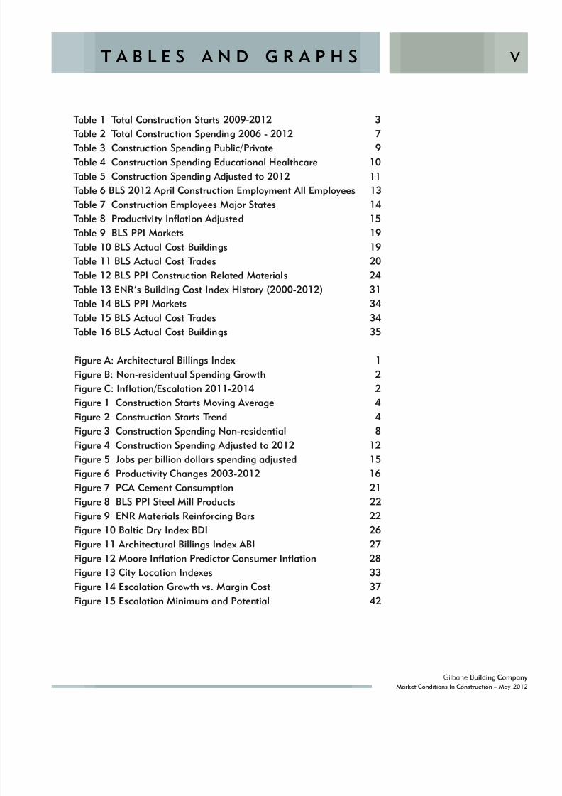
v T A B L E S A N D G R A P H S
Table 1 Total Construction Starts 2009-2012 3
Table 2 Total Construction Spending 2006 - 2012 7
Table 3 Construction Spending Public/Private 9
Table 4 Construction Spending Educational Healthcare 10
Table 5 Construction Spending Adjusted to 2012 11
Table 6 BLS 2012 April Construction Employment All Employees 13
Table 7 Construction Employees Major States 14
Table 8 Productivity Inflation Adjusted 15
Table 9 BLS PPI Markets 19
Table 10 BLS Actual Cost Buildings 19
Table 11 BLS Actual Cost Trades 20
Table 12 BLS PPI Construction Related Materials 24Table 13 ENR’s Building Cost Index History (2000-2012) 31
Table 14 BLS PPI Markets 34
Table 15 BLS Actual Cost Trades 34
Table 16 BLS Actual Cost Buildings 35
Figure A: Architectural Billings Index 1
Figure B: Non-residentual Spending Growth 2
Figure C: Inflation/Escalation 2011-2014 2
Figure 1 Construction Starts Moving Average 4
Figure 2 Construction Starts Trend 4Figure 3 Construction Spending Non-residential 8
Figure 4 Construction Spending Adjusted to 2012 12
Figure 5 Jobs per billion dollars spending adjusted 15
Figure 6 Productivity Changes 2003-2012 16
Figure 7 PCA Cement Consumption 21
Figure 8 BLS PPI Steel Mill Products 22
Figure 9 ENR Materials Reinforcing Bars 22
Figure 10 Baltic Dry Index BDI 26
Figure 11 Architectural Billings Index ABI 27
Figure 12 Moore Inflation Predictor Consumer Inflation 28Figure 13 City Location Indexes 33
Figure 14 Escalation Growth vs. Margin Cost 37
Figure 15 Escalation Minimum and Potential 42
8/10/2019 GBCo Market Conditions Spring 2012
http://slidepdf.com/reader/full/gbco-market-conditions-spring-2012 5/48
Gilbane Building Company
Market Conditions In Construction – May 2012
1
SUMMARY
SOME
ECONOMIC
FACTORS
AND
MARKET
FACTORS
SPECIFIC
TO
CONSTRUCTION
ARE
POSITIVE
: The Architectural Billing Indicator (ABI) accurately predicted a drop in spending from Q4 2011 through Q
2012. That may be ending. The ABI has been predicting growth starting in May’2012.
Even with the current decline in spending, the rate is still 9% above a year ago and 4% above last summe
Construction Spending should increase over 5% for 2012, more than 6% for non-residential buildings.
Contractors building costs for 2011 were much closer to labor and material cost increases, signaling amovement towards more normalized margins.
Sageworks Financial report on the construction industry shows contractor’s margins improved by 1% in2011, from 0.8% to 1.8%.
Industrial production related to construction is up 5 months in a row and 7.5% in 12 months
SOME ECONOMIC OR SPECIFIC MARKET FACTORS ARE STILL DECIDEDLY NEGATIVE:
Construction Employment increased seven times since February 2010, but dropped 6 times.
In 3 months since December we’ve gained only 5,000 jobs.
The 9 states with the most construction jobs lost 137,000 jobs over the last 4 months.
The Construction Starts trend since October is one of decline, hitting a 15-month low in February 2012.
Construction spending on public jobs is below the levels of a year ago.
After inflation adjustment we see construction volume has decreased 5 years in a row.
Portland Cement Association predicts cement consumption will increase only 0.5% in 2012. B ASED ON THE NEWEST DATA RELEASED SINCE THIS REPORT WAS COMPILED:
March Construction Starts were extremely high, emphasizing the volatility of this indicator.
Revised employment data for April shows jobs nearly flat since January 2012.
Our model shows spending below average in March 2012, as expected by the ABI indicator.
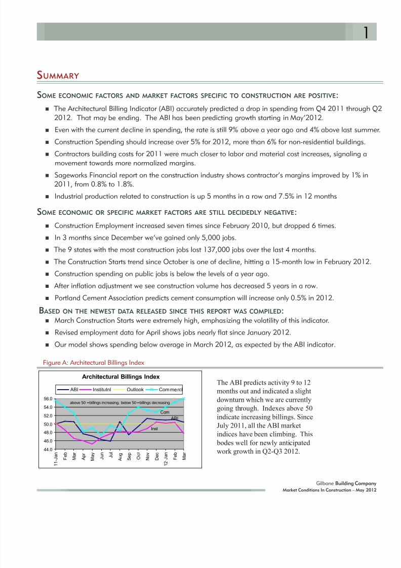
Figure A: Architectural Billings Index
Architectural Billings Index
ABI
Inst
Com
44.0
46.0
48.0
50.0
52.0
54.0
56.0
1 1 - J a n
F e b
M a r
A p r
M a y
J u n
J u l
A u g
S e p
O c t
N o v
D e c
1 2 - J a n
F e b
M a r
above 50 =billings increasing, below 50 =billings decreasing
ABI Institutnl Outlook Com mercl
The ABI predicts activity 9 to 12
months out and indicated a slight
downturn which we are currentlygoing through. Indexes above 50
indicate increasing billings. Since
July 2011, all the ABI market
indices have been climbing. This
bodes well for newly anticipated
work growth in Q2-Q3 2012.
8/10/2019 GBCo Market Conditions Spring 2012
http://slidepdf.com/reader/full/gbco-market-conditions-spring-2012 6/48
2
Gilbane Building Company
Market Conditions In Construction – May 2012
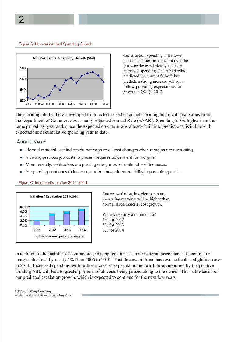
Figure B: Non-residentual Spending Growth
NonResidential Spending Growth ($bil)
520
540
560
580
J an-11 Mar-11 May-11 J ul-11 Sep-11 Nov-11 J an-12 Mar-12
The spending plotted here, developed from factors based on actual spending historical data, varies from
the Department of Commerce Seasonally Adjusted Annual Rate (SAAR). Spending is 8% higher than thesame period last year and, since the expected downturn was already built into predictions, is in line with
expectations of cumulative spending year to date.
A DDITIONALLY :
Normal material cost indices do not capture all cost changes when margins are fluctuating
Indexing previous job costs to present requires adjustment for margins.
More recently, contractors are passing along most of material cost increases.
As spending continues to increase, contractors gain more ability to pass along costs.
Figure C: Inflation/Escalation 2011-2014
Inflation / Escalation 2011-2014
0.0%
2.0%
4.0%
6.0%
8.0%
2011 2012 2013 2014
minimum and potential range
In addition to the inability of contractors and suppliers to pass along material price increases, contractor
margins declined by nearly 4% from 2006 to 2010. That downward trend has reversed with a slight increase
in 2011. Increased spending, with further increases expected in the near future, supported by the positive
trending ABI, will lead to greater portions of all costs being passed along to the owner. This is the basis for
our predicted escalation growth, which is expected to continue for the next few years.
Construction Spending still shows
inconsistent performance but over thelast year the trend clearly has been
increased spending. The ABI decline
predicted the current fall-off, but
predicts a strong increase will soon
follow, providing expectations for
growth in Q2-Q3 2012.
Future escalation, in order to capture
increasing margins, will be higher than
normal labor/material cost growth.
We advise carry a minimum of
4% for 2012
5% for 2013
6% for 2014

8/10/2019 GBCo Market Conditions Spring 2012
http://slidepdf.com/reader/full/gbco-market-conditions-spring-2012 7/48
3
Gilbane Building Company
Market Conditions In Construction – May 2012
CONSTRUCTION STARTS
Construction Starts published data gives monthly actual data and a seasonal adjusted annual rate (SAAR)
for each set of monthly Starts values. But the monthly values for Starts uctuate wildly. In fact, one ofthe most important things we can say about Construction Starts is that they can be extremely variable from
month to month, presumably dependent on the exact date that any new project gets listed.
SAAR based on monthly data in 2011 had variation from $380 billion to $470 billion (2010 varied from
$380billion to $450 billion). And yet, 2010 and 2011 nished within 2% of each other at $412 billion vs.
$421 billion. Any given month of data is far too volatile to predict the annual total. In the last two years of
data there have been at least 4 occasions when consecutive months have varied by an average 20% and as
high a difference as 25%. This causes unrealistic peaks and valleys in the data. Therefore, we do not use
month to month data to predict annual outcome.
One way to look at the data is to calculate a forecast based on the latest month, last 3 months and last 6months. One month trend data is always too volatile to predict the year, but shows the current monthly
trend; 3-month trends smooth out the data and give a near term trend and better prediction; and 6-month
trends atten the data even more and show a smoothed long-term trend.
Historically, we see only 7% of annual Starts in some months while we nd other months have 10% of
the annual Starts for the year. We see lowest Starts in November through February and highest Starts in
Jun through October It is not unusual to see huge increases or decreases in volume from month to month.
Historically, for non-residential buildings, there are 20% more Starts in Jun than in May and 30% more
Starts in October than November The SAAR factors are weakest during these periods and therefore at times
during the year the SAAR report can produce signicant variation from actual data and historical averages.
Our forecasting model is based on the actual data and historical averages.
Table 1 Total Construction Starts 2009-2012
TOTAL CONSTRUCTION STARTS Forecast 2012 based on
Actual Actual Actual 1 month 3 month Trend2009 2010 2011 actuals actuals predicion
Non-residential Buildings $ 167,955 $ 152,033 $ 154,782 $ 135,716 $ 141,140 $ 160,000
-9.5% 1.8% -12.3% -8.8% 3.4%
Residential Buildings $ 111,851 $ 119,360 $ 123,444 $ 146,499 $ 141,234 $ 145,000
6.7% 3.4% 18.7% 14.4% 17.5%
Non-building Construction $ 141,899 $ 141,078 $ 143,195 $ 117,342 $ 117,817 $ 120,000
-0.6% 1.5% -18.1% -17.7% -16.2%
Total Construction $ 421,705 $ 412,471 $ 421,421 $ 399,557 $ 400,191 $ 425,000
percent change yoy -2.2% 2.2% -5.2% -5.0% 0.8%
dollars in millions Feb’2012 Dec/Jan/Febforecast based on historical cumulative factors
8/10/2019 GBCo Market Conditions Spring 2012
http://slidepdf.com/reader/full/gbco-market-conditions-spring-2012 8/48
4
Gilbane Building Company
Market Conditions In Construction – May 2012
EXPECTATIONS AS OF A PRIL 2, 2012 BASED ON DATA THROUGH FEBRUARY : In the early part of the year Starts will seem to indicate no more than a $400,000 annual rate for the year
Non-building Construction, Infrastructure work may continue to decline
Total Starts will probably remain low due to steep declines in Non-building Infrastructure work
by May data we should see stable but slow growth in non-residential buildings.
The recent months of upward movement in the Architectural Billings Index should lead to growth in non-
residential Starts. Non-residential building Starts (our primary market) should end the year near $160 billion,
representing approximately 3% growth over 2011.
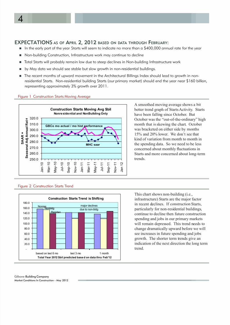
Figure 1 Construction Starts Moving Average
Construction Starts Moving Avg $bil
Nonresidential and NonBuilding Only
MHC saar
250.0
260.0
270.0
280.0
290.0
300.0
310.0
320.0
J a n - 1 0
M
a r - 1 0
M
a y - 1 0
J
u l - 1 0
S e p - 1 0
N o v - 1 0
J a n - 1 1
M
a r - 1 1
M
a y - 1 1
J
u l - 1 1
S e p - 1 1
N o v - 1 1
J a n 1 2
GBCo mo actual / mo hist performance
S A A R =
S e a s o n a l A d j A n n u a l R a t
Figure 2 Construction Starts Trend
Construction Starts Trend is Shifting
NonresNonbldg
major declines
due to non-bldgResiden
-
20.0
40.0
60.0
80.0
100.0
120.0
140.0
160.0
180.0
based on last 6 mo last 3 mo 1 month
Total Year 2012 $bil predicted base d on data thru Feb'12
A smoothed moving average shows a bit
better trend graph of Starts Activity. Starts
have been falling since October. ButOctober was the “out-of-the-ordinary” high
month that is skewing the chart. October
was bracketed on either side by months
15% and 20% lower. We don’t see that
kind of variation from month to month in
the spending data. So we need to be less
concerned about monthly uctuations in
Starts and more concerned about long-term
trends.
This chart shows non-building (i.e.,
infrastructure) Starts are the major factor
in recent declines. If construction Starts,
particularly for non-residential buildings,
continue to decline then future construction
spending and jobs in our primary markets
will remain depressed. This trend needs to
change dramatically upward before we willsee increases in future spending and jobs
growth. The shorter term trends give an
indication of the next direction the long term
trend.

8/10/2019 GBCo Market Conditions Spring 2012
http://slidepdf.com/reader/full/gbco-market-conditions-spring-2012 9/48
5
Gilbane Building Company
Market Conditions In Construction – May 2012
Inationary inuences have the effect of reducing the value of new Starts, and so, Starts at a rate lower than
the real ination rate would mean construction Starts in terms of building volume (not in terms of revenue)
are actually falling. If ination for the year comes in at 4%, then Starts need to be greater than 4% to realize
any growth.
CONSTRUCTION SPENDING
WHAT SHOULD WE EXPECT FOR 2012? HOW ARE WE DOING SO FAR ?
DOESN’T SOUND GOOD, DOES IT? OK, ’LET’S TAKE A LOOK .
Quoted from a February 7, 2012 post in my Gilbane blog
“it is widely agreed by many expert economists that we may experience a slowdown in the coming months…
(note- at this point December spending data had just been released).”
Quoted from a March 5, 2012 post in my Gilbane blog
“Earlier in 2011 the Architectural Billings Index showed work on the (architect’s) books declining. That
signaled an expected drop in construction 9 to 12 months out. We may be currently seeing this in the
declining new Starts….that could continue through April 2012….last year’s declining ABI billings indicated
Starts and spending would be lower for a period.”
Quoted from my Q4’2011 economics report
“The Architectural Billings Index has been signaling all year that we should expect further declines in
spending. A reliable indicator of work 9 to 12 months out, new Starts and spending results will always lag
the ABI.”
8/10/2019 GBCo Market Conditions Spring 2012
http://slidepdf.com/reader/full/gbco-market-conditions-spring-2012 10/48
Gilbane Building Company
Market Conditions In Construction – May 2012
6
First: It cannot be said this drop was UNEXPECTED. I’ve been
predicting the drop for a few months. Two leading indicators showed
an expected decline in Q1’ 2012 and previously reported jobs movement
followed suit. Now if the drop continues for 4 to 6 more months, that’s
unexpected.
Second: the Department of Commerce SAAR factor for January appears
to give a somewhat “too high” expectation for that month. On top of that,
December was an unusually strong month. So this is skewing the data
upon which all other news services report.
Third: January and February were the ONLY months that showed declines
in the last 7 months, and that’s undoubtedly because Q4’ 2011 was so
unusually strong and set a very high comparable. Furthermore, January
and February show spending at almost exactly the same rate, and bothstill show spending at a rate comfortably above Q3’ 2011.
My statistical monthly averages show from January to February the
monthly decline was only 0.2%, spending combined is 8% higher than the
same period last year and is within 0.1% of expectations cumulative year
to date. Since the bottom, spending has increased 9 out of 12 months and
the current rate for Jan-February is well above the rate last June, July, and
-August On an ination-adjusted basis, we’ve just had the best December,
January, and February period since ‘2008-’2009. It would appear so far
we are right on track.
The recently release CIRT (Construction Industry Round table) SentimentIndex Report, issued by FMI, representing collective input from
approximately 100 non-residential construction executives, includes these
data and responses: 42% of executives expect spending to improve only
modestly, from 0.5% to 2.5%, 26% expect little to no growth and 27%
expect spending declines. I do not share that sentiment.
I PRECICT THAT 2012 SPENDING FOR ALL CONSTRUCTION WILL BE $832 BILLION, A GROWTH OF 5.4%.
Given the most recent trends that take into consideration the 2011
midyear downturn in the ABI and a Q4 drop in new Starts, but thatmonthly spending rates increased in 9 out of the last 12 months,after factoring in an expected slowdown in the first quarter, my modelpredicts total spending will climb slowly for the remainder of the year,reflecting a growing ABI and slightly stronger economy, and will end the year 2012 at $832 billion spending for all construction, 5.4%above 2011. That represents a growth of only 2.2% after inflation.

8/10/2019 GBCo Market Conditions Spring 2012
http://slidepdf.com/reader/full/gbco-market-conditions-spring-2012 11/48
7
Gilbane Building Company
Market Conditions In Construction – May 2012
Table 2 Total Construction Spending 2006 - 2012
U.S. Total Construction Spending Summarytotals in billions U.S. dollars
Actual Forecast
2006 2007 2008 2009 2010 2011 2012
Non-residential Buildings 339.4 403.7 438.0 375.5 288.5 277.8 294.9
% change year over year 12.5% 18.9% 8.5% -14.3% -23.2% -3.7% 6.2%
Non-building heavy engr 207.9 248.3 271.8 273.3 266.4 266.6 274.9
12.4% 19.4% 9.5% 0.6% -2.5% 0.1% 3.1%
Residential 619.9 500.3 357.7 254.3 248.7 244.9 262.4
0.4% -19.3% -28.5% -28.9% -2.2% -1.5% 7.1%
Total 1167.2 1152.3 1067.5 903.1 803.6 789.2 832.2
5.7% -1.3% -7.4% -15.4% -11.0% -1.8% 5.4%
Residential includes new, remodeling, renovation and replacement work.
Source: U.S. Census Bureau, Department of Commerce.
Forecast 2012 - GBCo
Historically, the period of June through October shows the highest monthly rates of spending during the
year, all 5 months each over 9% of annual volume, with the highest monthly volume being reached in
August. Long-term averages show that spending in December, January and February each account for only
±7% of the annual volume. For example, in January and Feb, the lowest activity months of the year, history
leads us to expect to spend 7.0% of the total for the year. In August we expect to spend 9.5% of the total for
the year. If we see spending of $70 billion in January and $95 billion in August, this increase by $25 billion per month from January to August is seasonal, not an indication of growth. It simply indicates the rate
of spending in each of those months has reached the expected seasonal average rate for that month. Both
monthly values would predict the same year end total. We must use caution to not consider these increases
as an improvement in the rate of spending. The monthly rate-of-spending trends are holding through this
winter.
The months November through March have a high standard deviation from average and can produce wide
uctuations in year end data predicted from monthly data. However, the months of May through September
have a very low standard deviation and monthly data from that period gives a much more reliable year-end
prediction. Unfortunately, that means the current data for the past 4 months is among the least reliable to
predict the entire year.
Historical monthly activity can also be used to develop cumulative year-to-date data activity. This
eliminates some of the monthly uctuations and the total annual prediction gains more weight each month.
By September each year for 10 years, we had realized on average 75% total annual spending, with a
standard deviation of less than ±1%.
8/10/2019 GBCo Market Conditions Spring 2012
http://slidepdf.com/reader/full/gbco-market-conditions-spring-2012 12/48
8
Gilbane Building Company
Market Conditions In Construction – May 2012
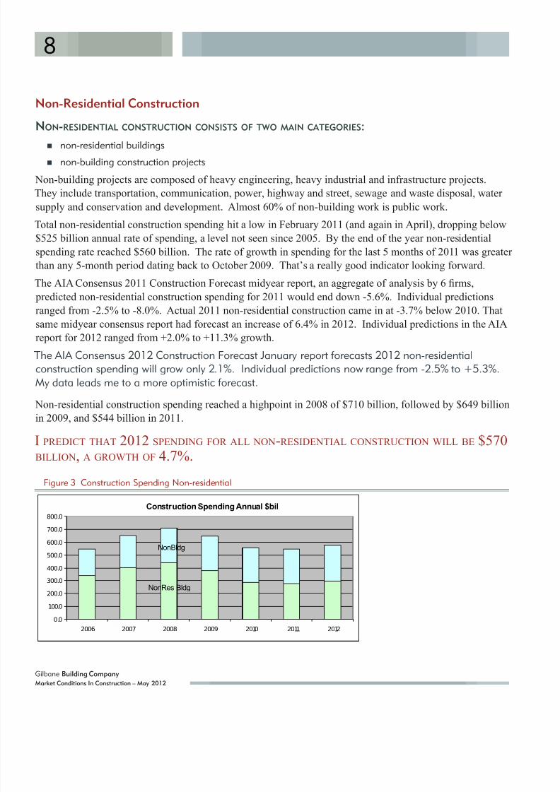
Non-Residential Construction
NON-RESIDENTIAL CONSTRUCTION CONSISTS OF TWO MAIN CATEGORIES:
non-residential buildings
non-building construction projects
Non-building projects are composed of heavy engineering, heavy industrial and infrastructure projects.
They include transportation, communication, power, highway and street, sewage and waste disposal, water
supply and conservation and development. Almost 60% of non-building work is public work.
Total non-residential construction spending hit a low in February 2011 (and again in April), dropping below
$525 billion annual rate of spending, a level not seen since 2005. By the end of the year non-residential
spending rate reached $560 billion. The rate of growth in spending for the last 5 months of 2011 was greater
than any 5-month period dating back to October 2009. That’s a really good indicator looking forward.
The AIA Consensus 2011 Construction Forecast midyear report, an aggregate of analysis by 6 rms,
predicted non-residential construction spending for 2011 would end down -5.6%. Individual predictions
ranged from -2.5% to -8.0%. Actual 2011 non-residential construction came in at -3.7% below 2010. That
same midyear consensus report had forecast an increase of 6.4% in 2012. Individual predictions in the AIA
report for 2012 ranged from +2.0% to +11.3% growth.
The AIA Consensus 2012 Construction Forecast January report forecasts 2012 non-residentialconstruction spending will grow only 2.1%. Individual predictions now range from -2.5% to +5.3%.My data leads me to a more optimistic forecast.
Non-residential construction spending reached a highpoint in 2008 of $710 billion, followed by $649 billion
in 2009, and $544 billion in 2011.
I PREDICT THAT 2012 SPENDING FOR ALL NON-RESIDENTIAL CONSTRUCTION WILL BE $570BILLION, A GROWTH OF 4.7%.
Figure 3 Construction Spending Non-residential
Construction Spending Annual $bil
NonRes Bldg
NonBldg
0.0
100.0
200.0
300.0
400.0
500.0
600.0
700.0
800.0
2006 2007 2008 2009 2010 2011 2012

8/10/2019 GBCo Market Conditions Spring 2012
http://slidepdf.com/reader/full/gbco-market-conditions-spring-2012 13/48
9
Gilbane Building Company
Market Conditions In Construction – May 2012
THE RECENTLY RELEASED CIRT SENTIMENT INDEX REPORT, REPRESENTING COLLECTIVE INPUT FROM NON-RESIDENTIAL CONSTRUCTION EXECUTIVES INCLUDES THESE RESPONSES:
More than 70% of executives expect the strongest increase of the year in Industrial/Petrochemical. Approx. 50% expect next strongest yearly increases in manufacturing and healthcare, but approximately
50% expect manufacturing and healthcare to remain the same or decline.
The educational sector still has the worst overall outlook 1 and 3 years out.
Non-Residential Buildings
Non-residential “buildings” construction spending reached a highpoint in 2008 at $438 billion, followed by
$376 billion in 2009, and $278 billion for 2011.
I PREDICT THAT 2012 SPENDING FOR NON-RESIDENTIAL BUILDINGS WILL BE $295 BILLION,
A GROWTH OF 6.2%.Private construction is predominantly residential. 97% of all residential work is private and constitutes
just under half of all private work. (A historical note: in 2005-2006, residential work constituted 70% of all
private work and more than half of all construction spending. For the last 3 years residential comprises
just less than 50% of private work and only 30% of all construction). Manufacturing (8%) and Commercial
(7.5%) are the next largest private “buildings” sectors. Non-buildings make up a large portion of private
work; ALL Power (17%) and Communication work (3.5%) is private work.
Private Construction spending reached a highpoint in 2006 at $912 billion and in 2011 was $506 billion.
I PREDICT THAT 2012 PRIVATE CONSTRUCTION SPENDING WILL BE $555 BILLION, AN INCREASE OF 9.8%, BUT STILL 40% BELOW THE PEAK .
Table 3 Construction Spending Public/Private
U.S. Total Construction Spendingtotals in billions U.S. dollars
Actual Forecast
2006 2007 2008 2009 2010 2011 2012
Private 911.8 863.4 758.8 588.1 500.4 505.7 555.0
% change year over year 4.8% -5.3% -12.1% -22.5% -14.9% 1.1% 9.8%
Public 255.4 288.9 308.7 315.0 303.2 283.5 277.2
9.0% 13.1% 6.9% 2.0% -3.7% -6.5% -2.2%
Total 1167.2 1152.3 1067.5 903.1 803.6 789.2 832.2
5.7% -1.3% -7.4% -15.4% -11.0% -1.8% 5.4%
Source: U.S. Census Bureau, Department of Commerce.
Forecast 2012 - GBCo
8/10/2019 GBCo Market Conditions Spring 2012
http://slidepdf.com/reader/full/gbco-market-conditions-spring-2012 14/48
10
Gilbane Building Company
Market Conditions In Construction – May 2012
The largest public construction markets are Highway and Educational. Those two markets alone represent
more than half of all public construction, followed by Transportation, a distant third, and Waste Disposal
fourth. All other markets together make up less than 30% of public work. Slight increases show up
in Highway from September through January, and Waste Disposal from October through February
Educational has been showing a steady decline for 6 months and Transportation, after deep drops since
2010, has been at since August.
Public Construction spending reached a highpoint in 2009 at $315 billion and in 2011 was $284 billion.
I PREDICT THAT 2012 PUBLIC CONSTRUCTION SPENDING WILL BE $277 BILLION, A DROP OF 2.2%, 12% BELOW THE 2009 PEAK .
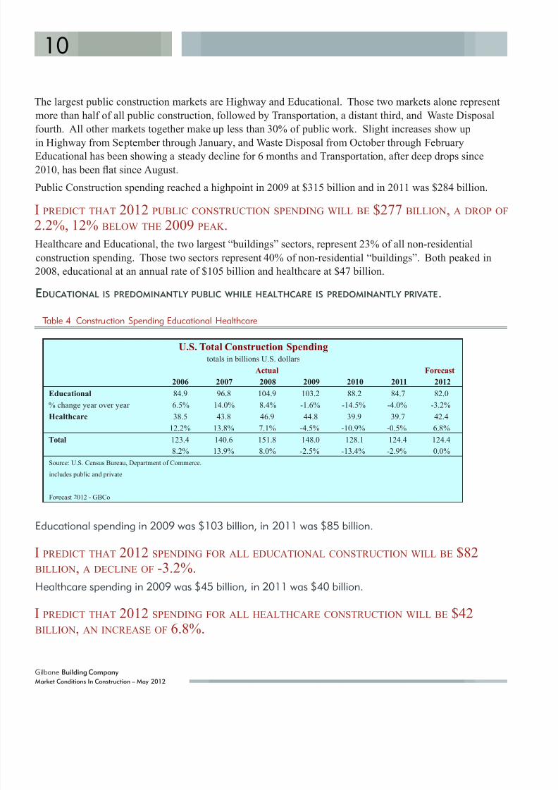
Healthcare and Educational, the two largest “buildings” sectors, represent 23% of all non-residential
construction spending. Those two sectors represent 40% of non-residential “buildings”. Both peaked in
2008, educational at an annual rate of $105 billion and healthcare at $47 billion.EDUCATIONAL IS PREDOMINANTLY PUBLIC WHILE HEALTHCARE IS PREDOMINANTLY PRIVATE.
Table 4 Construction Spending Educational Healthcare
U.S. Total Construction Spendingtotals in billions U.S. dollars
Actual Forecast
2006 2007 2008 2009 2010 2011 2012
Educational 84.9 96.8 104.9 103.2 88.2 84.7 82.0
% change year over year 6.5% 14.0% 8.4% -1.6% -14.5% -4.0% -3.2%
Healthcare 38.5 43.8 46.9 44.8 39.9 39.7 42.4
12.2% 13.8% 7.1% -4.5% -10.9% -0.5% 6.8%
Total 123.4 140.6 151.8 148.0 128.1 124.4 124.4
8.2% 13.9% 8.0% -2.5% -13.4% -2.9% 0.0%
Source: U.S. Census Bureau, Department of Commerce.
includes public and private
Forecast 2012 - GBCo
Educational spending in 2009 was $103 billion, in 2011 was $85 billion.
I PREDICT THAT 2012 SPENDING FOR ALL EDUCATIONAL CONSTRUCTION WILL BE $82BILLION, A DECLINE OF -3.2%.
Healthcare spending in 2009 was $45 billion, in 2011 was $40 billion.
I PREDICT THAT 2012 SPENDING FOR ALL HEALTHCARE CONSTRUCTION WILL BE $42BILLION, AN INCREASE OF 6.8%.
8/10/2019 GBCo Market Conditions Spring 2012
http://slidepdf.com/reader/full/gbco-market-conditions-spring-2012 15/48
11
Gilbane Building Company
Market Conditions In Construction – May 2012
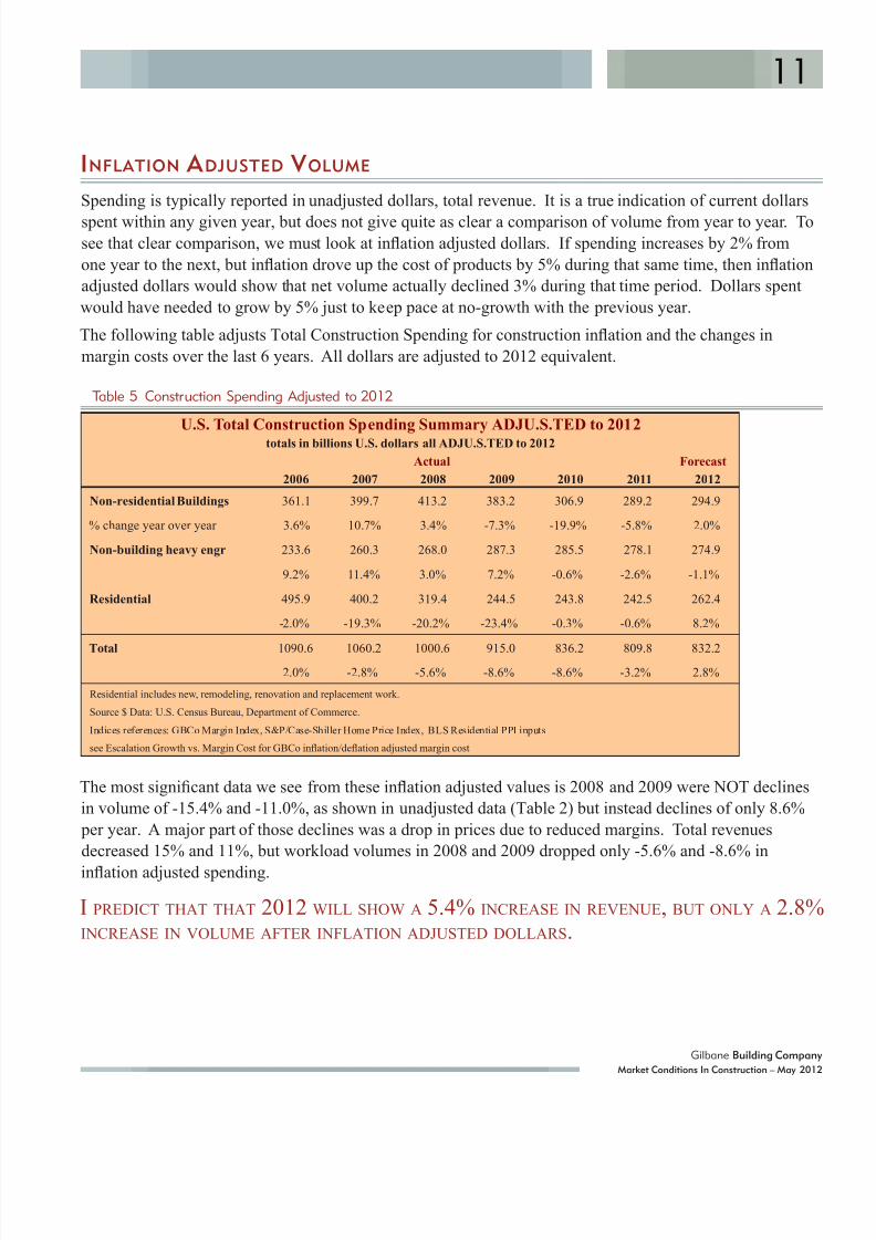
INFLATION A DJUSTED V OLUME
Spending is typically reported in unadjusted dollars, total revenue. It is a true indication of current dollars
spent within any given year, but does not give quite as clear a comparison of volume from year to year. Tosee that clear comparison, we must look at ination adjusted dollars. If spending increases by 2% from
one year to the next, but ination drove up the cost of products by 5% during that same time, then ination
adjusted dollars would show that net volume actually declined 3% during that time period. Dollars spent
would have needed to grow by 5% just to keep pace at no-growth with the previous year.
The following table adjusts Total Construction Spending for construction ination and the changes in
margin costs over the last 6 years. All dollars are adjusted to 2012 equivalent.
Table 5 Construction Spending Adjusted to 2012
U.S. Total Construction Spending Summary ADJU.S.TED to 2012totals in billions U.S. dollars all ADJU.S.TED to 2012
Actual Forecast
2006 2007 2008 2009 2010 2011 2012
Non-residential Buildings 361.1 399.7 413.2 383.2 306.9 289.2 294.9
% change year over year 3.6% 10.7% 3.4% -7.3% -19.9% -5.8% 2.0%
Non-building heavy engr 233.6 260.3 268.0 287.3 285.5 278.1 274.9
9.2% 11.4% 3.0% 7.2% -0.6% -2.6% -1.1%
Residential 495.9 400.2 319.4 244.5 243.8 242.5 262.4
-2.0% -19.3% -20.2% -23.4% -0.3% -0.6% 8.2%
Total 1090.6 1060.2 1000.6 915.0 836.2 809.8 832.2
2.0% -2.8% -5.6% -8.6% -8.6% -3.2% 2.8%
Residential includes new, remodeling, renovation and replacement work.
Source $ Data: U.S. Census Bureau, Department of Commerce.
Indices references: GBCo Margin Index, S&P/Case-Shiller Home Price Index, BLS Residential PPI inputs
see Escalation Growth vs. Margin Cost for GBCo ination/deation adjusted margin cost
The most signicant data we see from these ination adjusted values is 2008 and 2009 were NOT declines
in volume of -15.4% and -11.0%, as shown in unadjusted data (Table 2) but instead declines of only 8.6%
per year. A major part of those declines was a drop in prices due to reduced margins. Total revenues
decreased 15% and 11%, but workload volumes in 2008 and 2009 dropped only -5.6% and -8.6% in
ination adjusted spending.
I PREDICT THAT THAT 2012 WILL SHOW A 5.4% INCREASE IN REVENUE, BUT ONLY A 2.8%INCREASE IN VOLUME AFTER INFLATION ADJUSTED DOLLARS.
8/10/2019 GBCo Market Conditions Spring 2012
http://slidepdf.com/reader/full/gbco-market-conditions-spring-2012 16/48
12
Gilbane Building Company
Market Conditions In Construction – May 2012
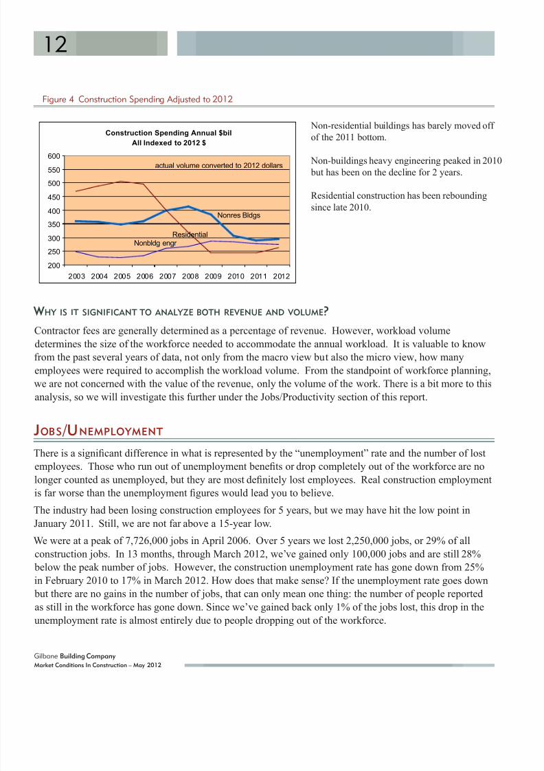
Figure 4 Construction Spending Adjusted to 2012
Construction Spending Annual $bilAll Indexed to 2012 $
Nonres Bldgs
Nonbldg engr Residential
200
250
300
350
400
450
500
550
600
2003 2004 2005 2006 2007 2008 2009 2010 2011 2012
actual volume converted to 2012 dollars
WHY IS IT SIGNIFICANT TO ANALYZE BOTH REVENUE AND VOLUME?
Contractor fees are generally determined as a percentage of revenue. However, workload volume
determines the size of the workforce needed to accommodate the annual workload. It is valuable to know
from the past several years of data, not only from the macro view but also the micro view, how many
employees were required to accomplish the workload volume. From the standpoint of workforce planning,
we are not concerned with the value of the revenue, only the volume of the work. There is a bit more to this
analysis, so we will investigate this further under the Jobs/Productivity section of this report.
JOBS /UNEMPLOYMENT
There is a signicant difference in what is represented by the “unemployment” rate and the number of lost
employees. Those who run out of unemployment benets or drop completely out of the workforce are no
longer counted as unemployed, but they are most denitely lost employees. Real construction employment
is far worse than the unemployment gures would lead you to believe.
The industry had been losing construction employees for 5 years, but we may have hit the low point in
January 2011. Still, we are not far above a 15-year low.
We were at a peak of 7,726,000 jobs in April 2006. Over 5 years we lost 2,250,000 jobs, or 29% of allconstruction jobs. In 13 months, through March 2012, we’ve gained only 100,000 jobs and are still 28%
below the peak number of jobs. However, the construction unemployment rate has gone down from 25%
in February 2010 to 17% in March 2012. How does that make sense? If the unemployment rate goes down
but there are no gains in the number of jobs, that can only mean one thing: the number of people reported
as still in the workforce has gone down. Since we’ve gained back only 1% of the jobs lost, this drop in the
unemployment rate is almost entirely due to people dropping out of the workforce.
Non-residential buildings has barely moved off
of the 2011 bottom.
Non-buildings heavy engineering peaked in 2010
but has been on the decline for 2 years.
Residential construction has been rebounding
since late 2010.
8/10/2019 GBCo Market Conditions Spring 2012
http://slidepdf.com/reader/full/gbco-market-conditions-spring-2012 17/48
13
Gilbane Building Company
Market Conditions In Construction – May 2012
While many workers are lost, the rst workers to be lost are typically those that represent the least value
to an organization, however, not all of the lost workers are “wanted turnover”. As the workload dwindled,
some of the workers that were let go or dropped out of the workforce had many years experience and were
highly trained. As a result, when work volume picks up there are going to be both general worker shortages
and as well as at least some shortage of these more valuable skilled workers. Over the next few years, when
work volume does pick up, this industry is going to be faced with a lack of available workers and shortage
of skilled, experienced workers. Both of those issues are going to DRIVE COSTS UP and QUALITY
DOWN due to the need to pay a premium for skilled workers and the necessity of training new workers in
their job and company procedures.
Table 6 BLS 2012 April Construction Employment All Employees
Industry: Construction Employment DataType:
ALL EMPLOYEES, THOU.S.ANDS
Year Jan Feb Mar Apr May Jun Jul Aug Sep Oct Nov Dec
2006 7601 7664 7689 7726 7713 7699 7712 7720 7718 7682 7666 7685
2007 7725 7626 7706 7686 7673 7687 7660 7610 7577 7565 7523 7490
2008 7481 7435 7401 7331 7282 7216 7161 7115 7042 6965 6810 6705
2009 6558 6448 6295 6151 6094 6007 5925 5846 5775 5717 5687 5654
2010 5593 5529 5552 5559 5518 5507 5491 5511 5492 5499 5488 5477
2011 5456 5489 5496 5495 5498 5495 5508 5498 5528 5519 5520 5546
2012 5564 5563 5560 5558
U.S. Bureau of labor Statistics
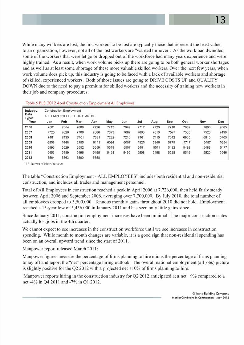
The table “Construction Employment - ALL EMPLOYEES” includes both residential and non-residential
construction, and includes all trades and management personnel.
Total of All Employees in construction reached a peak in April 2006 at 7,726,000, then held fairly steady
between April 2006 and September 2006, averaging over 7,700,000. By July 2010, the total number of
all employees dropped to 5,500,000. Tenuous monthly gains throughout 2010 did not hold. Employment
reached a 15-year low of 5,456,000 in January 2011 and has seen only little gains since.
Since January 2011, construction employment increases have been minimal. The major construction states
actually lost jobs in the 4th quarter.
We cannot expect to see increases in the construction workforce until we see increases in construction
spending. While month to month changes are variable, it is a good sign that non-residential spending has
been on an overall upward trend since the start of 2011.Manpower report released March 2011:
Manpower gures measure the percentage of rms planning to hire minus the percentage of rms planning
to lay off and report the “net” percentage hiring outlook. The overall national employment (all jobs) picture
is slightly positive for the Q2 2012 with a projected net +10% of rms planning to hire.
Manpower reports hiring in the construction industry for Q2 2012 anticipated at a net +9% compared to a
net -4% in Q4 2011 and -7% in Q1 2012.

8/10/2019 GBCo Market Conditions Spring 2012
http://slidepdf.com/reader/full/gbco-market-conditions-spring-2012 18/48
14
Gilbane Building Company
Market Conditions In Construction – May 2012
Manpower survey gures released in September 2011 indicated construction employment would decrease in
the fourth quarter That prediction was on target, with the top 9 states losing over 150,000 during the fourth
quarter.
Table 7 Construction Employees Major States
State Construction Employment # of Jobs
Four states account for 33% of ALL construction jobs.
current 12 mo last 4 mo
Texas 563,000 3,000 (41,000)
California 567,000 (3,000) (18,000)
Florida 319,000 (22,000) (15,000)
New York 301,000 (1,000) (25,000)
1,750,000 (23,000) (99,000)
Only ve other states have more than 150,000 construction jobs:current 12 mo last 4 mo
Pennsylvania 231,000 13,000 -
Illinios 190,000 (9,000) (29,000)
Virginia 182,000 500 (1,000)
North Carolina 177,000 6,000 1,000
Ohio 177,000 5,000 (9,000)
957,000 15,500 (38,000)
Where are the jobs?
Together these top 9 states make up 50%
of the national construction workforce.
The last (winter) report showed these
nine states combined had 39,000 more
jobs than a year ago. That has reversed
dramatically, showing the weakness in
jobs growth. Now they have 8,000 LESS
jobs than a year ago. And one year ago
total construction jobs had reached a 15
year low. The bad news is this group of
9 states lost 137,000 jobs in the 4 months
from Sep 2011 through Jan 2012. The
good news is the losses appear to have
been stemmed with the addition of 20,000
jobs in January.The big drop most probably reects the expected downturn
that was previously signaled by the falling ABI “work on the
boards” and construction Starts, among other indicators inthe middle of last year. National construction employment
totals increased by only 100,000 jobs during the same one year
period. Texas, which had been a jobs leader for the later half
of 2011, took the biggest drop.

8/10/2019 GBCo Market Conditions Spring 2012
http://slidepdf.com/reader/full/gbco-market-conditions-spring-2012 19/48
15
Gilbane Building Company
Market Conditions In Construction – May 2012
JOBS /PRODUCTIVITY
A long-term trend in productivity can be found by comparing the annual spending to the annual average
workforce. For this purpose we must use the ination adjusted spending, which will eliminate material,wage and margin ination/deation from the equation. Productivity is a measure of units per worker, not $
put in place per worker. This adjustment gives total spending in constant dollars and allows a comparison
to equal units. Therefore the following productivity analysis is based on put-in-place revenues, ination
adjusted to 2012 dollars, compared to actual manpower.
Table 8 Productivity Inflation Adjusted
Productivity Infation Adjusted 2002 2003 2004 2005 2006 2007 2008 2009 2010 2011 2012
Total Unadjusted $ Spending
848891 991 1,104 1,167 1,152 1,068 903 804 789 832
5.1% 11.2% 11.4% 5.7% -1.3% -7.4% -15% -11% -1.8% 5.4%
Total Spending 2012 $ 1,071 1,080 1,077 1,083 1,091 1,060 1,001 915 836 810 832
0.8% -0.2% 0.5% 0.7% -2.8% -5.6% -8.6% -8.6% -3.2% 2.8%
# jobs avg / yr mil lions 6,715 6,736 6,973 7,333 7,690 7,627 7,162 6,013 5,518 5,504 5,666
# jobs per billion$ unadjusted 7,919 7,558 7,033 6,641 6,588 6,619 6,709 6,658 6,867 6,974 6,808
# jobs per billion 2012 $ 6,268 6,238 6,472 6,774 7,051 7,194 7,158 6,572 6,599 6,797 6,808
productivity change 0.5% -3.6% -4.5% -3.9% -2.0% 0.5% 8.9% -0.4% -2.9% -0.2%
At rst glance, Figure 5 seems to indicate the number of jobs supported by $1 billion dollars of spending
declined from 2002 to 2006 (the thin black line). Fewer workers to perform the same unit volume of work
would indicate an increase in productivity. If productivity was increasing, then each succeeding year it
would take fewer workers to produce the same work volume and the number of jobs would be declining.But you can see that line would go counter to expectations. It shows increasing productivity in times
of increasing workload. What’s missing in that analysis is the dollar volume of work put in place is not
ination adjusted, so it indicates work $ value, but not true work unit volume.
Figure 5 Jobs per billion dollars spending adjusted
JOBS per $bil ajusted to 2012$
#jobs per$bi
unadjustedl #jobs per $bil
in 2012$
5,500
6,000
6,500
7,000
7,500
8,000
2002 2003 2004 2005 2006 2007 2008 2009 2010 2011 2012
# of Jobs needed to support $1 billion spending
To get the real picture of
productivity changes we must
adjust all dollars to the same
point in time, here adjusted to
2012$. Once we’ve done that,we see the adjusted data in Figure
5 (the thicker blue line) shows
productivity declining in lock-step
with rapid volume growth and
improving as work volume drops.
8/10/2019 GBCo Market Conditions Spring 2012
http://slidepdf.com/reader/full/gbco-market-conditions-spring-2012 20/48
16
Gilbane Building Company
Market Conditions In Construction – May 2012
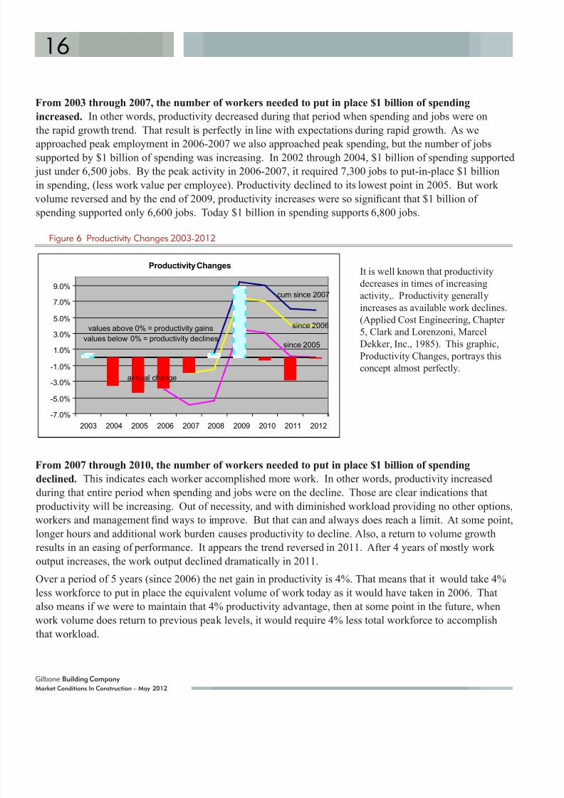
From 2003 through 2007, the number of workers needed to put in place $1 billion of spending
increased. In other words, productivity decreased during that period when spending and jobs were on
the rapid growth trend. That result is perfectly in line with expectations during rapid growth. As we
approached peak employment in 2006-2007 we also approached peak spending, but the number of jobs
supported by $1 billion of spending was increasing. In 2002 through 2004, $1 billion of spending supported
just under 6,500 jobs. By the peak activity in 2006-2007, it required 7,300 jobs to put-in-place $1 billion
in spending, (less work value per employee). Productivity declined to its lowest point in 2005. But work
volume reversed and by the end of 2009, productivity increases were so signicant that $1 billion of
spending supported only 6,600 jobs. Today $1 billion in spending supports 6,800 jobs.
Figure 6 Productivity Changes 2003-2012
Productivity Changes
annual change
cum since 2007
since 2005
since 2006
-7.0%
-5.0%
-3.0%
-1.0%
1.0%
3.0%
5.0%
7.0%
9.0%
2003 2004 2005 2006 2007 2008 2009 2010 2011 2012
values above 0% = productivity gains
values below 0% = productivity declines
From 2007 through 2010, the number of workers needed to put in place $1 billion of spending
declined. This indicates each worker accomplished more work. In other words, productivity increased
during that entire period when spending and jobs were on the decline. Those are clear indications that
productivity will be increasing. Out of necessity, and with diminished workload providing no other options,
workers and management nd ways to improve. But that can and always does reach a limit. At some point,
longer hours and additional work burden causes productivity to decline. Also, a return to volume growth
results in an easing of performance. It appears the trend reversed in 2011. After 4 years of mostly work
output increases, the work output declined dramatically in 2011.
Over a period of 5 years (since 2006) the net gain in productivity is 4%. That means that it would take 4%
less workforce to put in place the equivalent volume of work today as it would have taken in 2006. That
also means if we were to maintain that 4% productivity advantage, then at some point in the future, when
work volume does return to previous peak levels, it would require 4% less total workforce to accomplish
that workload.
It is well known that productivity
decreases in times of increasing
activity,. Productivity generally
increases as available work declines.
(Applied Cost Engineering, Chapter
5, Clark and Lorenzoni, Marcel
Dekker, Inc., 1985). This graphic,
Productivity Changes, portrays this
concept almost perfectly.
8/10/2019 GBCo Market Conditions Spring 2012
http://slidepdf.com/reader/full/gbco-market-conditions-spring-2012 21/48
17
Gilbane Building Company
Market Conditions In Construction – May 2012
As workload begins to increase in coming years, net productivity gains will decline somewhat. This net
affect cannot go unaddressed. The results of productivity declines are either decreased total output (if
workforce remains constant) or increased workforce needed (if total workload remains constant). Even with
the drop in 2011, fewer workers are needed currently to accomplish the same work volume as compared to
any time since 2005. However, that is already changing.
Realistically, I would expect that over the next few years, each year work volume increases we will
experience some slight erosion from the productivity gains. That means when we do once again recover to
the spending levels of years past, we will not recover to the number of jobs in years past. This erosion can
be offset by signicant technological and process advancements. I expect some of what we saw in 2009 can
be attributed to those two issues.
Earlier I asked, Why is it significant to analyze both revenue and volume?
Contractor fees are often determined as a percentage of revenue. However, workload volume is used for
planning the size of the workforce needed to accommodate the annual workload. It is valuable to know
from the past several years of data how many employees were required to accomplish the workload volume.
From the viewpoint of workforce determination, we should not be concerned with the value of the revenue,
only the volume of the work.
A S AN EXAMPLE:
At the peak of construction, a building cost $12 million and took 100 men/yr to build. Today that samebuilding could potentially cost as little as $10 million to build. Does it take 20% less men/yr to build it? No,certainly not. That would be the fallacy of trying to determine jobs needed based on revenue.
The building has not changed, only its cost changed. It still has the same amount of steel and concrete and
brick and windows. The only thing we can say is we’ve had an improvement of 4% in productivity. Therefore the workforce today will be 4% lower. Using revenue as a basis we might be led to think we need 20% fewerworkers. That points to the value to base workers needed on inflation adjusted volume, not direct annualrevenue.
How quickly can we recover from a 30% decline in the workforce?
The most rapid expansion in the workforce during the last 10 years was the period from mid-2003 to
mid-2006. In that 36-month period, the construction labor workforce expanded by 1,000,000 jobs, 15%.
Therefore, during the strongest period of expansion in the last 10 years, the workforce expanded by only
15% over 3 years, or an average of 28,000 jobs per month. What’s signicant is that ination adjusted
volume increased by only 10%. Such a signicant workforce expansion led to measurable lost productivity.Even if we could realize a similar rate of growth, which was associated with a high rate of economic
expansion, it would take 6 years to recover more than 2 million lost jobs. At this accelerated rate the
workforce would not return to previous levels before 2017. That is a very unlikely scenario, since it would
require uninterrupted elevated economic expansion. It is highly unlikely we will see the workforce return
to previous levels within 6 years. Furthermore, if we experience uninterrupted economic expansion at this
level for the next 6 years, productivity is going to plummet erasing all of the gains realized in the last few
years and more.
8/10/2019 GBCo Market Conditions Spring 2012
http://slidepdf.com/reader/full/gbco-market-conditions-spring-2012 22/48
18
Gilbane Building Company
Market Conditions In Construction – May 2012
The rate of employment growth may be a valid concern for the following reason; if spending and jobs are
to remain balanced and return to normal, then both the rate of expansion in construction spending and the
rate of growth in the workforce needs to be approximately equal in the coming years. If the rate of spending
growth exceeds a normal the rate of growth, it will produce an extremely active market, there will be worker
shortages and productivity will drop. Also, when that occurs, it leads to rapidly increasing prices and
elevated margins.
CONSTRUCTION COSTS GENERAL
Industrial production related to construction is up 5 months in a row and is up over 7.5% in 12 months since
February 2011.
Fabricated metal products industry reported production is up, prices paid are lower and Backlog of
Orders is up.
Of items used in construction, copper, copper wire, copper pipe, aluminum, diesel fuel and plastics are all
still UP in price over the last 3 months. Structural shapes are down in price over 3 months.
Concrete and steel, the major drivers of building structure cost, are both experiencing low cost increases.
Concrete contractor pricing is up less than 1.5% over the year and more recently is down. Fabricated
structural products are up less than 2.5% over the year.
In March, Ken Simonson, AGC Chief Economist, said he expects materials prices to range from 4% to 9%
during the year, but to end at 5% to 6% increases for the year 2012. Labor is expected to nish the year up
1.5% to 2.5%.
Manufacturing capacity utilization had been uctuating between 76% and 77% since November 2010. In
July it increased just above 77%, by October it was approaching 78% and since December it has been near
79%. Typically, the capacity utilization index needs to be consistently above 80 before we see an expansion
of construction spending in the manufacturing sector. Spending in this sector is still down 23% from last
year. That will keep prices in that sector depressed.
M ATERIAL PRICE MOVEMENT
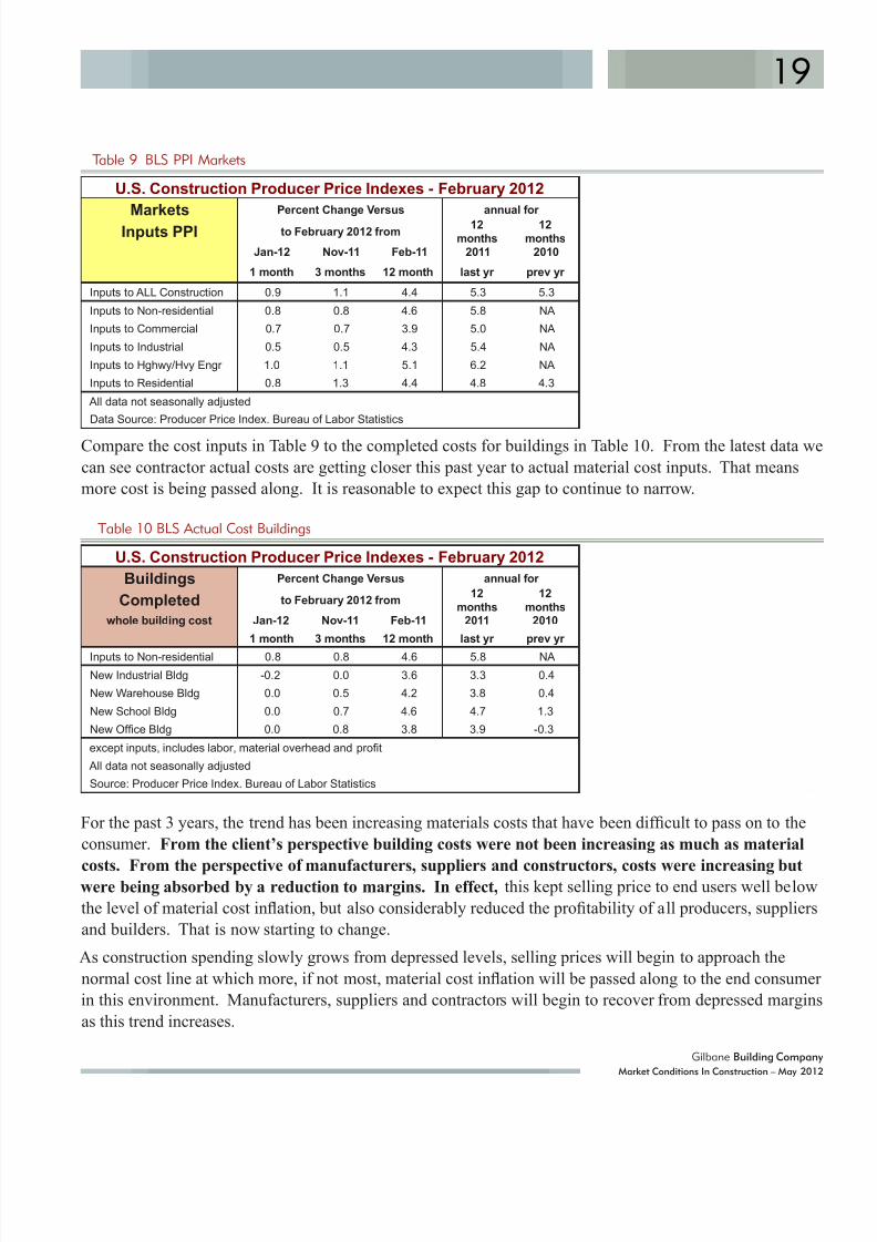
The overall Producer Price Index (PPI) for February 2012 shows cost for construction materials are up 4.4%
in the last 12 months. Costs for material inputs to non-residential construction are up 4.6% in the last 12months. Prices for completed buildings are up on average 4.0%.
8/10/2019 GBCo Market Conditions Spring 2012
http://slidepdf.com/reader/full/gbco-market-conditions-spring-2012 23/48
19
Gilbane Building Company
Market Conditions In Construction – May 2012
Table 9 BLS PPI Markets
U.S. Construction Producer Price Indexes - February 2012
MarketsPercent Change Versus annual for
Inputs PPI to February 2012 from12
months12
months Jan-12 Nov-11 Feb-11 2011 2010
1 month 3 months 12 month last yr prev yr
Inputs to ALL Construction 0.9 1.1 4.4 5.3 5.3
Inputs to Non-residential 0.8 0.8 4.6 5.8 NA
Inputs to Commercial 0.7 0.7 3.9 5.0 NA
Inputs to Industrial 0.5 0.5 4.3 5.4 NA
Inputs to Hghwy/Hvy Engr 1.0 1.1 5.1 6.2 NA
Inputs to Residential 0.8 1.3 4.4 4.8 4.3
All data not seasonally adjusted
Data Source: Producer Price Index. Bureau of Labor Statistics
Compare the cost inputs in Table 9 to the completed costs for buildings in Table 10. From the latest data we
can see contractor actual costs are getting closer this past year to actual material cost inputs. That means
more cost is being passed along. It is reasonable to expect this gap to continue to narrow.
Table 10 BLS Actual Cost Buildings
U.S. Construction Producer Price Indexes - February 2012
Buildings Percent Change Versus annual for
Completed to February 2012 from12
months12
monthswhole building cost Jan-12 Nov-11 Feb-11 2011 2010
1 month 3 months 12 month last yr prev yr
Inputs to Non-residential 0.8 0.8 4.6 5.8 NA
New Industrial Bldg -0.2 0.0 3.6 3.3 0.4
New Warehouse Bldg 0.0 0.5 4.2 3.8 0.4
New School Bldg 0.0 0.7 4.6 4.7 1.3
New Ofce Bldg 0.0 0.8 3.8 3.9 -0.3
except inputs, includes labor, material overhead and prot
All data not seasonally adjusted
Source: Producer Price Index. Bureau of Labor Statistics
For the past 3 years, the trend has been increasing materials costs that have been difcult to pass on to the
consumer. From the client’s perspective building costs were not been increasing as much as material
costs. From the perspective of manufacturers, suppliers and constructors, costs were increasing butwere being absorbed by a reduction to margins. In effect, this kept selling price to end users well below
the level of material cost ination, but also considerably reduced the protability of all producers, suppliers
and builders. That is now starting to change.
As construction spending slowly grows from depressed levels, selling prices will begin to approach the
normal cost line at which more, if not most, material cost ination will be passed along to the end consumer
in this environment. Manufacturers, suppliers and contractors will begin to recover from depressed margins
as this trend increases.

8/10/2019 GBCo Market Conditions Spring 2012
http://slidepdf.com/reader/full/gbco-market-conditions-spring-2012 24/48
20
Gilbane Building Company
Market Conditions In Construction – May 2012
Table 11 BLS Actual Cost Trades
U.S. Construction Producer Price Indexes - February 2012
TradesPercent Change Versus annual for
Non-residential to February 2012 from12
months12
monthswhole trade bid cost Jan-12 Nov-11 Feb-11 2011 2010
1 month 3 months 12 month last yr prev yr
Inputs to Non-residential 0.8 0.8 4.6 5.8 NA
Concrete -0.2 -0.5 1.1 1.3 0.4
Roong 0.0 0.7 4.2 4.3 -1.9
Electrical 0.8 1.2 4.1 3.8 1.1
Plumbing / HVAC -0.1 0.8 4.3 3.6 1.7
except inputs, includes labor, material overhead and prot
All data not seasonally adjusted
Source: Producer Price Index. Bureau of Labor Statistics
I expect whole building costs to rise, but a bit slower than material/labor ination.
Indicators are pointing to growth signs and that will eventually lead to a more normal bidding environment.
That in turn will allow builders to pass along ever greater percentages of cost increases. Concrete trades
over the last year increased prices only about 1%, but Roong Electrical and Plumbing / HVAC trades all
increased prices on average 4%.
NOTABLE MATERIALS CHANGES OVER THE LAST 12 MONTHS THROUGH FEBRUARY :
diesel fuel +14%
gypsum products +15%
copper and brass shapes -11%
steel pipe +10%
asphalt paving +11%
CEMENT / CONCRETE
Portland Cement Association (PCA) reports the volume of cement demand as an indicator of economic
activity. It is a reliable coincident indicator.
Nearly two-thirds of U.S. cement consumption occurs in the six months between May and October. Rising
consumption and prices leading into summer can lead to large shifts in demand and seasonal pricing andis not an indicator of long term growth but only reects periodic seasonal uc0tuating consumption rates.
Look at total annual volumes for trends.
Cement ProductionIn 2008 U.S. cement plants were operating at a capacity utilization of 82%. In Fall 2011, cement plant
capacity utilization, considered depressed, was 60%. The rate of decline in consumption helps explain the
60% capacity utilization. In 2010, cement production and consumption hit a 28-year low.
8/10/2019 GBCo Market Conditions Spring 2012
http://slidepdf.com/reader/full/gbco-market-conditions-spring-2012 25/48
21
Gilbane Building Company
Market Conditions In Construction – May 2012
Figure 7 PCA Cement Consumption
millions
metric tons
2010 = 28yr
low
0
20
40
60
80
100
120
140
2005 2007 2009 2011 2013
Cement Consumption
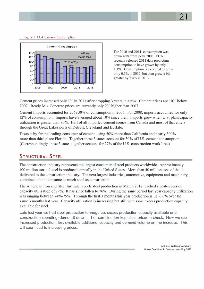
Cement prices increased only 1% in 2011 after dropping 3 years in a row. Cement prices are 10% below2007. Ready Mix Concrete prices are currently only 2% higher than 2007.
Cement Imports accounted for 25%-30% of consumption in 2006. For 2008, imports accounted for only
12% of consumption. Imports have averaged about 10% since then. Imports grow when U.S. plant capacity
utilization is greater than 80%. Half of all imported cement comes from Canada and most of that enters
through the Great Lakes ports of Detroit, Cleveland and Buffalo.
Texas is by far the leading consumer of cement, using 50% more than California and nearly 300%
more than third place Florida. Together these 3 states account for 30% of U.S. cement consumption.
(Correspondingly, these 3 states together account for 27% of the U.S. construction workforce).
STRUCTURAL STEEL
The construction industry represents the largest consumer of steel products worldwide. Approximately
100 million tons of steel is produced annually in the United States. More than 40 million tons of that is
delivered to the construction industry. The next largest industries, automotive, equipment and machinery,
combined do not consume as much steel as construction.
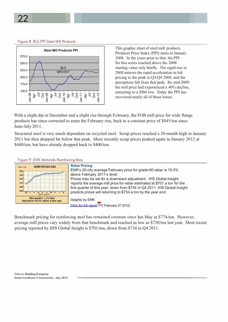
The American Iron and Steel Institute reports steel production in March 2012 reached a post-recession
capacity utilization of 79%. It has since fallen to 76%. During the same period last year capacity utilization
was ranging between 74%-75%. Through the rst 3 months this year production is UP 6.6% over the
same 3 months last year. Capacity utilization is increasing but still with some excess production capacityavailable for steel.
Late last year we had steel production tonnage up, excess production capacity available andconstruction spending (demand) down. That combination kept steel prices in check. Now we seeincreased production, less available additional capacity and demand volume on the increase. Thiswill soon lead to increasing prices.
For 2010 and 2011, consumption wasdown 46% from peak 2008. PCA
recently released 2011 data predicting
consumption to have grown by only
1.1%. Consumption is expected to grow
only 0.5% in 2012, but then grow a bit
greater by 7.4% in 2013.
8/10/2019 GBCo Market Conditions Spring 2012
http://slidepdf.com/reader/full/gbco-market-conditions-spring-2012 26/48
8/10/2019 GBCo Market Conditions Spring 2012
http://slidepdf.com/reader/full/gbco-market-conditions-spring-2012 27/48
23
Gilbane Building Company
Market Conditions In Construction – May 2012
COPPER
Copper material prices hit an all-time high of $4.60/lb in February 2011, up 25% from October 2010. By
September 2011 the price dropped back to $3.10/lb. The price as of April 4, 2012 was just under $3.85/lb,15% below where it was a year ago.
WHAT MAKES COPPER SO IMPORTANT TO WATCH?
Copper is a leading economic indicator that has rarely (if ever) failed to indicate the direction of world
economies. When copper rises in price, world economies are leading into expansion. When copper drops
in price, a decline in world economies very quickly follows. Copper prices and the U.S. workforce move
almost perfectly together. Also, because copper is so widely used in buildings, and manufacturing facilities
must be built to see a big increase in production, copper demand precedes and is an excellent predictor of
industrial production 12 months out.
For a visual representation of the copper prices, visit:
http://metalprices.com/PubCharts/PublicCharts.aspx?metal=cu&type=L&weight=LB&days=60&size=M&bg=&cs=1011&cid=0
What drives copper prices up or down? Unlike some other metals, it is not speculation. Quite often it is
demand. Increasing demand = increasing prices. When demand wanes, prices drop. Analysts predict
copper will average $4.00/lb in 2012.
WHAT AFFECT DO COPPER PRICE CHANGES HAVE ON THE COST OF OUR PROJECTS?
ROUGHLY SPEAKING, COPPER MATERIAL IS ABOUT:
10% of an Electrical contract or 1% of cost of project
5% of an HVAC contract or 0.6% of cost of project
10% of a Plumbing contract or 0.3% of cost of project
So, for an average project, copper material can represent approximately 2% of the total cost of the project.
Therefore, a 25% increase in the cost of copper will increase the cost of a project by 0.5%.
There may be exceptions. For example, if copper is 2% of the total cost of the typical project, it is probably
4% to 5% of total cost on a heavy mechanical/electrical project, like a data center. So a 25% increase in the
cost of copper increases the total cost of a data center by 1% to 1.5%. For a copper roof, material is 65% of
total cost and can represent ~1% of typical project cost.

8/10/2019 GBCo Market Conditions Spring 2012
http://slidepdf.com/reader/full/gbco-market-conditions-spring-2012 28/48
24
Gilbane Building Company
Market Conditions In Construction – May 2012
PRODUCER PRICE INDEX
The February 2012 2011 Producer Price Index for Material Inputs to Construction increased 1.1% over the
last 3 months and is up 4.4% over the past 12 months.
The February 2012 PPI for Material Inputs to Non-residential Construction decreased 0.8% over the last 3months and is up 4.6% over the past 12 months.
PPI for Trade Contractors nal costs and Whole Building nal costs is UP, but up only about 4% in 12
months. See Materials Price Movement for Contractor Installed Prices and Finished Building Prices.
Table 12 BLS PPI Construction Related Materials
U.S. Construction Producer Price Indexes - February 2012
Materials Percent Change Versus annual for
to February 2012 from12
months
12
months Jan-12 Nov-11 Feb-11 2011 2010
1 month 3 months 12 month last yr prev yr
Summary
Inputs to ALL Construction 0.9 1.1 4.4 5.3 5.3
Inputs to Non-residential 0.8 0.8 4.6 5.8 NA
Commodities
Cement -2.4 1.3 2.2 1.1 -6.0
Iron & Steel Scrap -6.2 3.5 -4.5 11.1 38.9
Manufactured Materials
Diesel Fuel 3.0 -2.0 14.5 20.2 26.4
Asphalt Paving 2.5 4.3 11.3 8.4 4.4
Asphalt Roong -0.5 -2.4 -1.9 2.6 1.9
Ready Mix Concrete -0.2 1.0 1.5 0.6 -1.2
Concrete Block & Brick -0.1 0.3 1.8 1.1 -1.1
Precast Conc Products 0.1 0.2 0.1 2.6 1.0
Building Brick 0.2 -3.4 -2.9 -2.6 -0.3
Copper / Brass Mill Shapes 5.9 4.7 -11.2 -9.3 11.8
Aluminum Mill Shapes 1.9 -0.8 -0.8 0.1 11.6
Steel Mill Products 0.6 1.3 4.0 11.3 12.5
Steel Pipe and Tube -0.8 4.9 10.0 12.1 19.6
Fab. Structural Steel 1.9 1.2 2.5 4.4 1.9
Fab. Bar Joists and Rebar 2.4 0.7 1.4 2.8 -0.3
Gypsum Products 5.1 12.0 15.2 -1.5 3.2
Insulation Materials 0.4 3.3 5.0 5.4 4.6Lumber and Plywood 1.7 2.3 -0.7 -0.8 5.7
Sheet Metal Products -0.5 -2.1 2.4 5.8 4.0
All data not seasonally adjusted
Source: Producer Price Index. Bureau of Labor Statistics
The primary factor keeping total costs down right now is high level of competition for a slowly increasing
volume of new work. The price asked for subcontract work and for nished buildings is slowly starting to
catch up with the rate of material cost increases.

8/10/2019 GBCo Market Conditions Spring 2012
http://slidepdf.com/reader/full/gbco-market-conditions-spring-2012 29/48
25
Gilbane Building Company
Market Conditions In Construction – May 2012
THE PPI FOR ITEMS THAT CONTRIBUTED THE MOST TO THE 3 MONTH AND YEARLY CHANGE INCLUDED:
Diesel fuel prices dropped 2% recently but climbed 14% over the last year Asphalt paving is up 4% in 3 months and up 11% over the year
Gypsum products rose 12% in 3 months and 15% over the year
Steel pipe and tube rose 5% in 3 months and but rose 10% over the year
Is the PPI for Construction Materials = Escalation? NO!
IS THE MOVEMENT OF THE PPI A GOOD INDICATOR OF FUTURE ESCALATION? NO!
Indexes like the PPI MTRLS deal ONLY with materials costs or prices charged at the producer level. They
do not include delivery, equipment, installation, or markups. In fact, they do not even reect the retail pricecharged to contractors. Nor do they reect the cost of services provided by the GC or CM.
Total project cost encompasses all of these other costs. Trade Contractor PPI and Whole Building PPI
doesn’t give us any details about the retail price of the materials used, but it does include all of the
contractors costs incurred for delivery, equipment for installation, labor for installation and markups on the
nal product delivered to the consumer, the building.
The PPI for construction materials IS NOT an indicator of construction ination. It is missing the selling
price. In 2010, the PPI for construction inputs was up 5.3% but the selling price was at. In 2009 PPI for
Inputs was at but construction ination as measured by cost of buildings was down 8%-10%.
Construction Starts and construction spending are still near 10-year lows, and therefore there is little workavailable out for bid, forcing contractors to remain extremely competitive. As a result, they areunable
to pass on all cost increases to clients. This has the effect of keeping selling price low, reducing both
contractors and producers margins. In some cases margins may be reduced to a loss just to get work.
Construction cost escalation is moving closer to track in line with the PPI for construction materials. But it
will take continued increases in the levels of activity to enforce the narrowing of the gap between the two.
I do not expect cost escalation to track in-line with PPI for at least 1 to 2 years. Until then, do notbase building cost growth on the increase in construction materials PPI.
8/10/2019 GBCo Market Conditions Spring 2012
http://slidepdf.com/reader/full/gbco-market-conditions-spring-2012 30/48
26
Gilbane Building Company
Market Conditions In Construction – May 2012
THE B ALTIC DRY INDEX
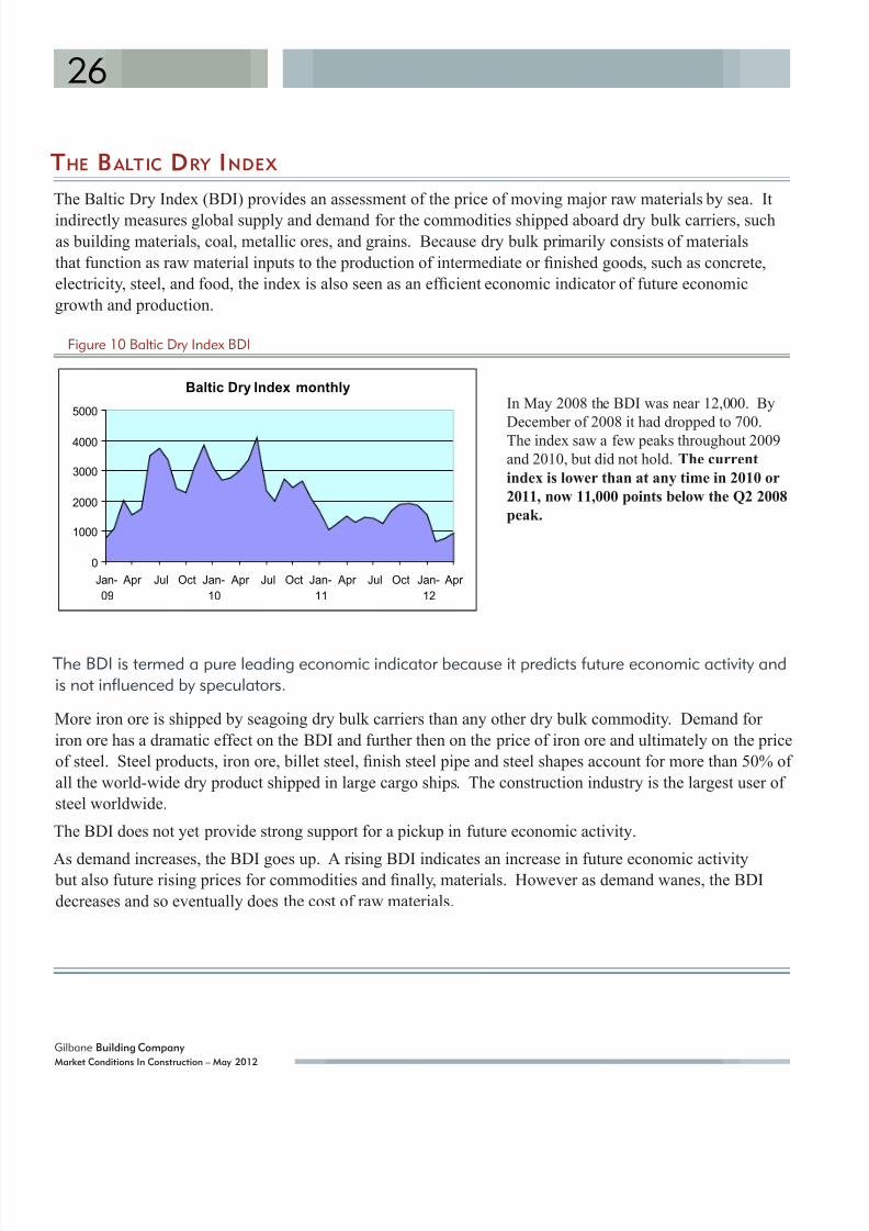
The Baltic Dry Index (BDI) provides an assessment of the price of moving major raw materials by sea. It
indirectly measures global supply and demand for the commodities shipped aboard dry bulk carriers, suchas building materials, coal, metallic ores, and grains. Because dry bulk primarily consists of materials
that function as raw material inputs to the production of intermediate or nished goods, such as concrete,
electricity, steel, and food, the index is also seen as an efcient economic indicator of future economic
growth and production.
Figure 10 Baltic Dry Index BDI
Baltic Dry Index monthly
0
1000
2000
3000
4000
5000
Jan-
09
Apr Jul Oct Jan-
10
Apr Jul Oct Jan-
11
Apr Jul Oct Jan-
12
Apr
The BDI is termed a pure leading economic indicator because it predicts future economic activity andis not influenced by speculators.
More iron ore is shipped by seagoing dry bulk carriers than any other dry bulk commodity. Demand for
iron ore has a dramatic effect on the BDI and further then on the price of iron ore and ultimately on the price
of steel. Steel products, iron ore, billet steel, nish steel pipe and steel shapes account for more than 50% of
all the world-wide dry product shipped in large cargo ships. The construction industry is the largest user of
steel worldwide.
The BDI does not yet provide strong support for a pickup in future economic activity.
As demand increases, the BDI goes up. A rising BDI indicates an increase in future economic activity but also future rising prices for commodities and nally, materials. However as demand wanes, the BDI
decreases and so eventually does the cost of raw materials.
In May 2008 the BDI was near 12,000. By
December of 2008 it had dropped to 700.
The index saw a few peaks throughout 2009
and 2010, but did not hold. The current
index is lower than at any time in 2010 or
2011, now 11,000 points below the Q2 2008
peak.
8/10/2019 GBCo Market Conditions Spring 2012
http://slidepdf.com/reader/full/gbco-market-conditions-spring-2012 31/48
27
Gilbane Building Company
Market Conditions In Construction – May 2012
A RCHITECTURAL B ILLINGS INDEX
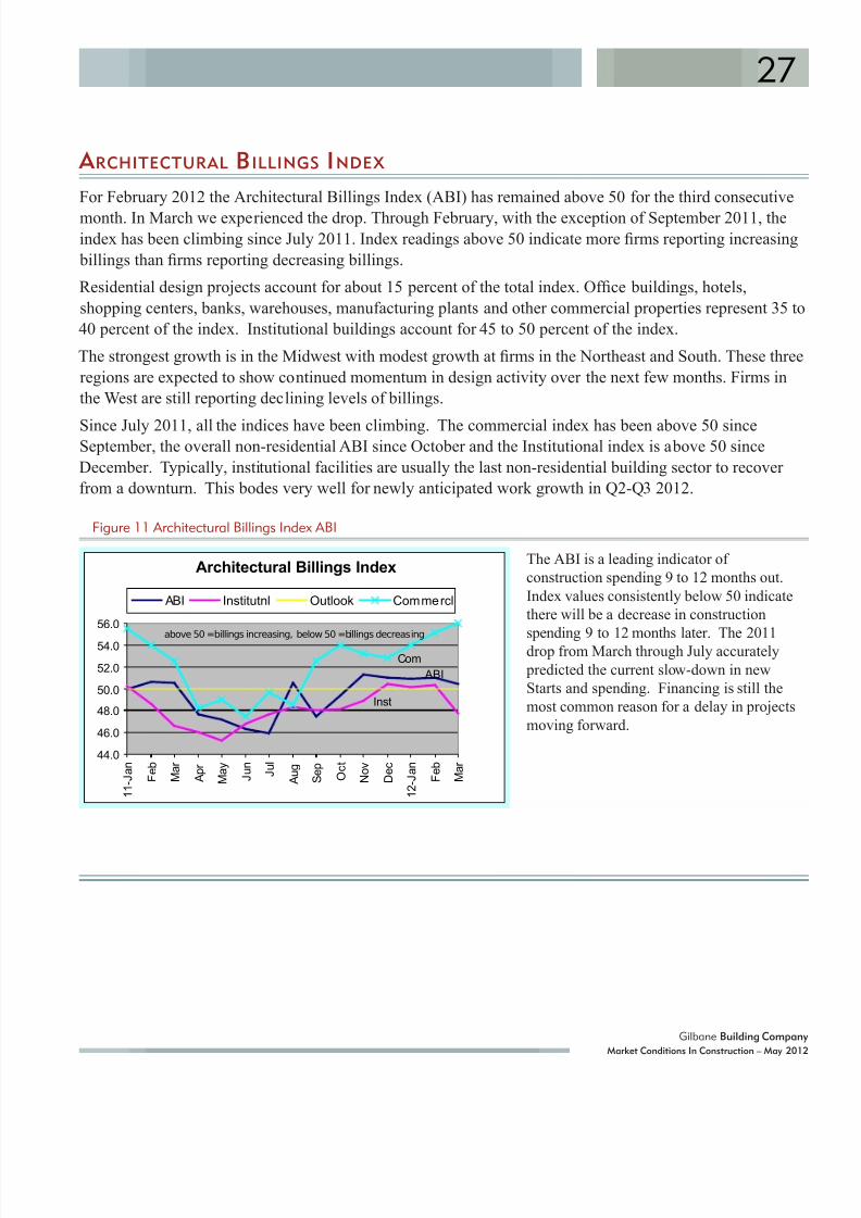
For February 2012 the Architectural Billings Index (ABI) has remained above 50 for the third consecutive
month. In March we experienced the drop. Through February, with the exception of September 2011, theindex has been climbing since July 2011. Index readings above 50 indicate more rms reporting increasing
billings than rms reporting decreasing billings.
Residential design projects account for about 15 percent of the total index. Ofce buildings, hotels,
shopping centers, banks, warehouses, manufacturing plants and other commercial properties represent 35 to
40 percent of the index. Institutional buildings account for 45 to 50 percent of the index.
The strongest growth is in the Midwest with modest growth at rms in the Northeast and South. These three
regions are expected to show continued momentum in design activity over the next few months. Firms in
the West are still reporting declining levels of billings.
Since July 2011, all the indices have been climbing. The commercial index has been above 50 sinceSeptember, the overall non-residential ABI since October and the Institutional index is above 50 since
December. Typically, institutional facilities are usually the last non-residential building sector to recover
from a downturn. This bodes very well for newly anticipated work growth in Q2-Q3 2012.
Figure 11 Architectural Billings Index ABI
Architectural Billings Index
ABI
Inst
Com
44.0
46.0
48.0
50.0
52.0
54.0
56.0
1 1 - J a n
F e b
M a r
A p r
M a y
J u n
J u l
A u g
S e p
O c t
N o v
D e c
1 2 - J a n
F e b
M a r
above 50 =billings increasing, below 50 =billings decreasing
ABI Institutnl Outlook Commercl
The ABI is a leading indicator of
construction spending 9 to 12 months out.
Index values consistently below 50 indicate
there will be a decrease in construction
spending 9 to 12 months later. The 2011drop from March through July accurately
predicted the current slow-down in new
Starts and spending. Financing is still the
most common reason for a delay in projects
moving forward.
8/10/2019 GBCo Market Conditions Spring 2012
http://slidepdf.com/reader/full/gbco-market-conditions-spring-2012 32/48
28
Gilbane Building Company
Market Conditions In Construction – May 2012
CONSUMER INFLATION / DEFLATION
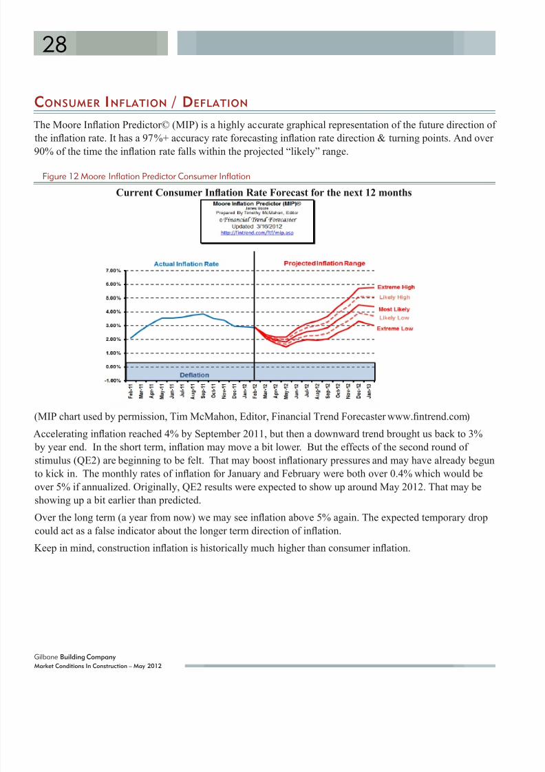
The Moore Ination Predictor© (MIP) is a highly accurate graphical representation of the future direction of
the ination rate. It has a 97%+ accuracy rate forecasting ination rate direction & turning points. And over90% of the time the ination rate falls within the projected “likely” range.
Figure 12 Moore Inflation Predictor Consumer Inflation
Current Consumer Ination Rate Forecast for the next 12 months
(MIP chart used by permission, Tim McMahon, Editor, Financial Trend Forecaster www.ntrend.com)
Accelerating ination reached 4% by September 2011, but then a downward trend brought us back to 3%
by year end. In the short term, ination may move a bit lower. But the effects of the second round of
stimulus (QE2) are beginning to be felt. That may boost inationary pressures and may have already begun
to kick in. The monthly rates of ination for January and February were both over 0.4% which would be
over 5% if annualized. Originally, QE2 results were expected to show up around May 2012. That may be
showing up a bit earlier than predicted.
Over the long term (a year from now) we may see ination above 5% again. The expected temporary drop
could act as a false indicator about the longer term direction of ination.
Keep in mind, construction ination is historically much higher than consumer ination.

8/10/2019 GBCo Market Conditions Spring 2012
http://slidepdf.com/reader/full/gbco-market-conditions-spring-2012 33/48
29
Gilbane Building Company
Market Conditions In Construction – May 2012
CONSTRUCTION INFLATION FORECAST
Construction ination, based on several decades of trends, is double consumer ination. Since mid-2009that long term trend has not held up. Recent construction ination continues to be inuenced primarily by
bid margins which have been low due to low work volume. If it holds true that long-term trends eventually
return to the norm, we may be headed for some serious construction ination down the road.
From January through April 2011 consumer ination shot up to 3%. At that time expectations were that
consumer ination would continue to climb through the year, potentially to a range just above 5% with a
drop back to 3% expected by May 2012. We see now that it reached near 4% by September and returned to
3% by year end and may go lower by May. But that short-term downward trend should then turn upwards
and move closer to 5% a year from now.
Normally we would expect construction ination to come in near double that range. Construction materials
currently are below that trend. However, keep in mind, because of current low demand, prices are being
held down. Construction materials ination is low year to date, but increased signicantly in the latest
month. As demand increases in coming months, construction ination may climb rapidly.
Until construction spending returns to normal, I expect total construction escalation cost passed on to
owners might be somewhat subdued, perhaps no more than 4%. Subdued nished building prices will be
inuenced by aggressive bidding. This will change quickly as bidding volume increases.
SOME S IGNS A HEAD
The Institute for Supply Management (ISM) report released April 2, 2012, shows the national Purchasing
Manager’s Index (PMI) is 53.4%. It is growing stronger. PMI values above 42.5 indicate overall economic
expansion. Index values above 50 indicate expansion in the manufacturing sector. Fabricated metal
products industry reported production is up, prices paid are lower and Backlog of Orders is up.
The ISM Non Manufacturing Index (NMI) measures economic activity in several industries (including
construction) not covered in the manufacturing sector. The NMI for March is 56.0, down from February,
but still growing, although at a slower rate. The New Orders and Backlog Indexes declined for the month.
A respondent from the construction industry commented, “We are starting to see the private sector building
again.”
Industrial production related to construction is up 5 months in a row and is up over 7.5% in 12 months since
February 2011.
The Conference Board Leading Economic Index (LEI) is up 5 months in a row through February. After 5
months of strong growth, the Employment Trend Index (ETI) turned down slightly in March.
The Economic Cycle Research Institute (ECRI) U.S. Weekly Leading Index of economic growth predicts
8/10/2019 GBCo Market Conditions Spring 2012
http://slidepdf.com/reader/full/gbco-market-conditions-spring-2012 34/48
30
Gilbane Building Company
Market Conditions In Construction – May 2012
economic activity 2 to 3 quarters out. This index was positive from December 2010 through August 2011,
when it turned mildly negative. It turned stronger negative in October. But since November the WLI has
been on the increase and since January has been increasing strongly.
The Architectural Billings Index (ABI) is a leading indicator of construction spending 9 to 12 months out.
Since July 2011, all the ABI market indices have been climbing. The commercial index has been above 50
since September, the overall non-residential ABI since October and the Institutional index is above 50 since
December. Typically, institutional facilities are usually the last non-residential building sector to recover
from a downturn. This bodes very well for newly anticipated work growth in Q2-Q3 2012.
Manpower reports hiring in the construction industry for Q2 2012 anticipated at a net +9% compared to a
net -4% in Q4 2011 and -7% in Q1 2012.
Construction Starts hit a 12-month low in September, but hit an unusual high in October, likely reecting
volatility from month to month. Starts have trended downward since October hitting a 15 month low in
February. This may be strongly inuenced by a sharp drop in non-building Starts.
The FMI rst quarter Non-residential Construction Index Report (NRCI) is now 58.1, is up almost 8 points
from the previous quarter. FMI’s index of the overall economy provided the strongest improvement in the
overall index.
ENR INDEX
The March 2012 Engineering News Record Building Cost Index (ENR-BCI) is 5144, up 0.6% year to
date. However, the winter months historically show very low growth while the summer months show rapid
growth. In times of 4% annual escalation expect the winter rate to be -2% to +2%, while the summer rate
will be +6% to +7%. The ENR BCI index increased 3.7% in 2010 and 2.8% in 2011.
THE ENR-BCI IS ONE OF THE MOST WELL-KNOWN AND MOST WIDELY USED BUILDING COST INDICES.HOWEVER, ITS LONG-TERM STRENGTHS CAN ALSO BE WEAKNESSES, PARTICULARLY IN TIMES OF FLUCTUATING SELLING PRICES BECAUSE:
It is made up of a small shopping basket of labor and materials. Therefore it is not always the bestrepresentation of all building types, which can vary considerably in composition.
That shopping basket includes no representation for any Mechanical, Electrical or Plumbing items, whichcan comprise 30%-50% of the cost of the building. In many cases the shopping basket comprises less than 20% of the building cost.
Building materials differ widely in rate and timing of cost growth and can dramatically affect the costof projects. In 2009 while structural steel products declined in price by -10% to -15%, copper productsincreased in price by 40%+.
ENR-BCI does not take into consideration bid prices, so it often does not represent the final cost ofbuildings. Bid prices are referred to as Selling Price, and this is not included in the ENR-BCI. Sellingprices show increased or reduced margin bids due to market activity.
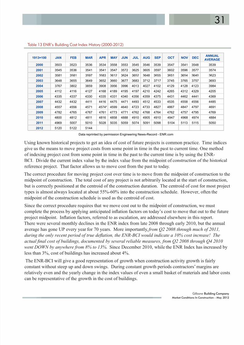
8/10/2019 GBCo Market Conditions Spring 2012
http://slidepdf.com/reader/full/gbco-market-conditions-spring-2012 35/48
31
Gilbane Building Company
Market Conditions In Construction – May 2012
Table 13 ENR’s Building Cost Index History (2000-2012)
1913=100 JAN FEB MAR APR MAY JUN JUL AUG SEP OCT NOV DECANNUAL
AVERAGE2000 3503 3523 3536 3534 3558 3553 3545 3546 3539 3547 3541 3548 3539
2001 3545 3536 3541 3541 3547 3572 3625 3605 3597 3602 3596 3577 3574
2002 3581 3581 3597 3583 3612 3624 3652 3648 3655 3651 3654 3640 3623
2003 3648 3655 3649 3652 3660 3677 3683 3712 3717 3745 3765 3757 3693
2004 3767 3802 3859 3908 3956 3996 4013 4027 4102 4129 4128 4123 3984
2005 4112 4116 4127 4168 4189 4195 4197 4210 4242 4265 4312 4329 4205
2006 4335 4337 4330 4335 4331 4340 4356 4359 4375 4431 4462 4441 4369
2007 4432 4432 4411 4416 4475 4471 4493 4512 4533 4535 4558 4556 4485
2008 4557 4556 4571 4574* 4599 4640 4723 4733 4827 4867 4847 4797 4691
2009 4782 4765 4767 4761 4773 4771 4762 4768 4764 4762 4757 4795 4769
2010 4800 4812 4811 4816 4858 4888 4910 4905 4910 4947 4968 4974 4884
2011 4969 5007 5010 5028 5035 5059 5074 5091 5098 5104 5113 5115 5050
2012 5120 5122 5144
Data reprinted by permission Engineering News-Record - ENR.com
Using known historical projects to get an idea of cost of future projects is common practice. Time indices
give us the means to move project costs from some point in time in the past to current time. One method
of indexing project cost from some point in time in the past to the current time is by using the ENR-
BCI. Divide the current index value by the index value from the midpoint of construction of the historical
reference project. That factor allows us to move cost from the past to today.
The correct procedure for moving project cost over time is to move from the midpoint of construction to the
midpoint of construction. The total cost of any project is not arbitrarily located at the start of construction, but is correctly positioned at the centroid of the construction duration. The centroid of cost for most projec
types is almost always located at about 55%-60% into the construction schedule. However, often the
midpoint of the construction schedule is used as the centroid of cost.
Since the correct procedure requires that we move cost out to the midpoint of construction, we must
complete the process by applying anticipated ination factors on today’s cost to move that out to the future
project midpoint. Ination factors, referred to as escalation, are addressed elsewhere in this report.
There were several monthly declines in the ENR index from late 2008 through early 2010, but the annual
average has gone UP every year for 70 years. More importantly, from Q2 2008 through much of 2011,
during the only recent period of true deation, the ENR-BCI would indicate a 10% cost increase! The
actual nal cost of buildings, documented by several reliable measures, from Q2 2008 through Q4 2010went DOWN by anywhere from 8% to 13%. Since December 2010, while the ENR Index has increased by
less than 3%, cost of buildings has increased about 4%.
The ENR-BCI will give a good representation of growth when construction activity growth is fairly
constant without steep up and down swings. During constant growth periods contractors’ margins are
relatively even and the yearly change in the index values of even a small basket of materials and labor costs
can be representative of the growth in the cost of buildings.

8/10/2019 GBCo Market Conditions Spring 2012
http://slidepdf.com/reader/full/gbco-market-conditions-spring-2012 36/48
32
Gilbane Building Company
Market Conditions In Construction – May 2012
Whenever we have very active periods or very depressed periods of construction activity, contractor
selling prices rise or fall accordingly and the ENR-BCI, since it does not track selling price, cannot reect
accurately what affect selling price had on the cost of buildings during those periods. Nonetheless, the
ENR-BCI is often relied upon as an indicator of cost movement over time.
We’ve just gone through a period of three to four years during which margins were rst inated and then
deeply depressed, transitioning dramatically from peak to trough. If you rely solely on the ENR-BCI to
index the cost of buildings from, during or across that period of time, you may end up with indexed cost
results that are grossly in error. If you were to select a time period between Q2 2008 and today, you could
be overstating the future cost of a building by approximately 15% to 20%. You must at the very least take
into consideration the selling price of buildings, past and present.
Selling prices are not captured in the ENR Index. For a procedure to adjust for actual selling prices see the
Indexing – Addressing the Fluctuation in Margins section of this report, and refer to the graph Escalation
Growth vs. Margin Cost. This is particularly important for those of you using cost modeling tools suchas Gilbane’s CostAdvisor.
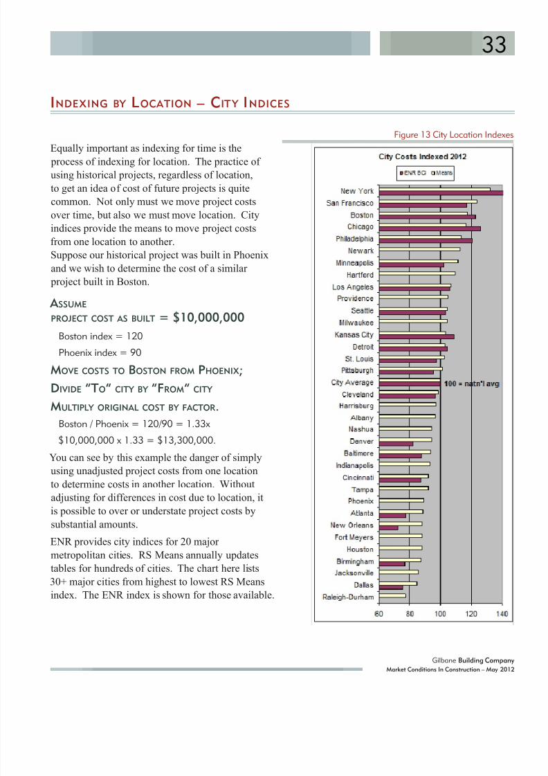
8/10/2019 GBCo Market Conditions Spring 2012
http://slidepdf.com/reader/full/gbco-market-conditions-spring-2012 37/48
33
Gilbane Building Company
Market Conditions In Construction – May 2012
INDEXING BY LOCATION – CITY INDICES
Equally important as indexing for time is the
process of indexing for location. The practice of
using historical projects, regardless of location,
to get an idea of cost of future projects is quite
common. Not only must we move project costs
over time, but also we must move location. City
indices provide the means to move project costs
from one location to another.
Suppose our historical project was built in Phoenix
and we wish to determine the cost of a similar project built in Boston.
A SSUME PROJECT COST AS BUILT = $10,000,000
Boston index = 120
Phoenix index = 90
MOVE COSTS TO BOSTON FROM PHOENIX;
DIVIDE “TO” CITY BY “FROM” CITY
MULTIPLY ORIGINAL COST BY FACTOR.Boston / Phoenix = 120/90 = 1.33x
$10,000,000 x 1.33 = $13,300,000.
You can see by this example the danger of simply
using unadjusted project costs from one location
to determine costs in another location. Without
adjusting for differences in cost due to location, it
is possible to over or understate project costs by
substantial amounts.
ENR provides city indices for 20 majormetropolitan cities. RS Means annually updates
tables for hundreds of cities. The chart here lists
30+ major cities from highest to lowest RS Means
index. The ENR index is shown for those available.
Figure 13 City Location Indexes

8/10/2019 GBCo Market Conditions Spring 2012
http://slidepdf.com/reader/full/gbco-market-conditions-spring-2012 38/48
34
Gilbane Building Company
Market Conditions In Construction – May 2012
SELLING PRICE
Selling price is the total price at which a contractor is willing to bid to win a project, even if that selling
price eliminates all prot from the bid.
Few ination or material/labor cost predictors address the issue of bidders lowering margins to win work
and hence lowering what is known as Selling Price. Selling price is dramatically affected by economic
conditions such as market volume and contractor booked revenue. When market volume is low, contractor’s
margin, or Selling Price, comes down. As business volume picks up, and once contractors secure more work,
even if material prices stay low, contractors begin to increase their selling price.
Table 14 BLS PPI Markets
U.S. Construction Producer Price Indexes - February 2012
Markets Percent Change Versus annual for
Inputs PPI to February 2012 from12
months12
months Jan-12 Nov-11 Feb-11 2011 2010
1 month 3 months 12 month last yr prev yr
Inputs to ALL Construction 0.9 1.1 4.4 5.3 5.3
Inputs to Non-residential 0.8 0.8 4.6 5.8 NA
Inputs to Commercial 0.7 0.7 3.9 5.0 NA
Inputs to Industrial 0.5 0.5 4.3 5.4 NA
Inputs to Hghwy/Hvy Engr 1.0 1.1 5.1 6.2 NA
Inputs to Residential 0.8 1.3 4.4 4.8 4.3
All data not seasonally adjusted
Data Source: Producer Price Index. Bureau of Labor Statistics
We are currently in a slow period predicted by both the Construction Starts gures reported by McGraw Hill
and the Architectural Billings Index published by the AIA. Both indices in Q4 2011 indicated declining
construction activity for the next 6 to 9 months. However, monthly rate of spending is still well above
levels of the last 18 months. Although it may be several years before building markets return to pre-
recession levels, at least we can say the rate of activity is increasing.
Table 15 BLS Actual Cost Trades
U.S. Construction Producer Price Indexes - February 2012
Trades Percent Change Versus annual for
Non-residential to February 2012 from 12 months 12 months
whole trade bid cost Jan-12 Nov-11 Feb-11 2011 2010 1 month 3 months 12 month last yr prev yr
Inputs to Non-residential 0.8 0.8 4.6 5.8 NA
Concrete -0.2 -0.5 1.1 1.3 0.4
Roong 0.0 0.7 4.2 4.3 -1.9
Electrical 0.8 1.2 4.1 3.8 1.1
Plumbing / HVAC -0.1 0.8 4.3 3.6 1.7
except inputs, includes labor, material overhead and prot
All data not seasonally adjusted | Source: Producer Price Index. Bureau of Labor Statistics
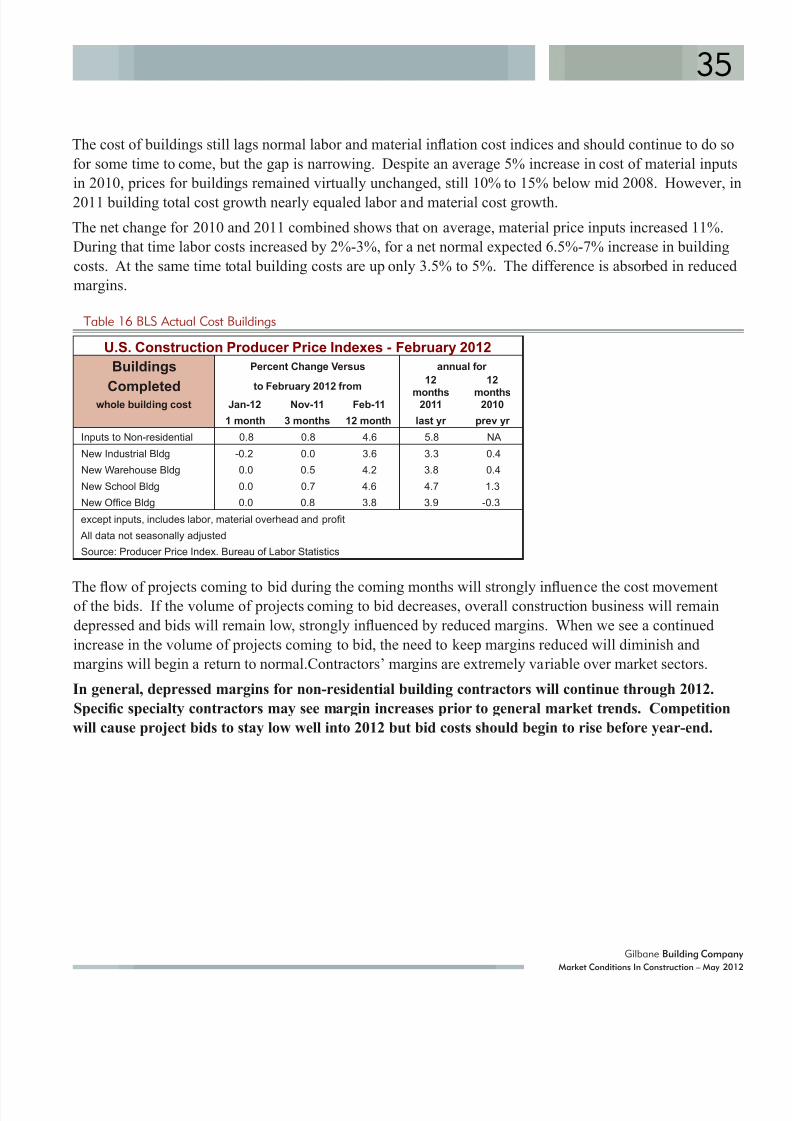
8/10/2019 GBCo Market Conditions Spring 2012
http://slidepdf.com/reader/full/gbco-market-conditions-spring-2012 39/48
35
Gilbane Building Company
Market Conditions In Construction – May 2012
The cost of buildings still lags normal labor and material ination cost indices and should continue to do so
for some time to come, but the gap is narrowing. Despite an average 5% increase in cost of material inputs
in 2010, prices for buildings remained virtually unchanged, still 10% to 15% below mid 2008. However, in
2011 building total cost growth nearly equaled labor and material cost growth.
The net change for 2010 and 2011 combined shows that on average, material price inputs increased 11%.
During that time labor costs increased by 2%-3%, for a net normal expected 6.5%-7% increase in building
costs. At the same time total building costs are up only 3.5% to 5%. The difference is absorbed in reduced
margins.
Table 16 BLS Actual Cost Buildings
U.S. Construction Producer Price Indexes - February 2012
Buildings Percent Change Versus annual for
Completedto February 2012 from
12
months
12
monthswhole building cost Jan-12 Nov-11 Feb-11 2011 2010
1 month 3 months 12 month last yr prev yr
Inputs to Non-residential 0.8 0.8 4.6 5.8 NA
New Industrial Bldg -0.2 0.0 3.6 3.3 0.4
New Warehouse Bldg 0.0 0.5 4.2 3.8 0.4
New School Bldg 0.0 0.7 4.6 4.7 1.3
New Ofce Bldg 0.0 0.8 3.8 3.9 -0.3
except inputs, includes labor, material overhead and prot
All data not seasonally adjusted
Source: Producer Price Index. Bureau of Labor Statistics
The ow of projects coming to bid during the coming months will strongly inuence the cost movementof the bids. If the volume of projects coming to bid decreases, overall construction business will remain
depressed and bids will remain low, strongly inuenced by reduced margins. When we see a continued
increase in the volume of projects coming to bid, the need to keep margins reduced will diminish and
margins will begin a return to normal.Contractors’ margins are extremely variable over market sectors.
In general, depressed margins for non-residential building contractors will continue through 2012.
Specic specialty contractors may see margin increases prior to general market trends. Competition
will cause project bids to stay low well into 2012 but bid costs should begin to rise before year-end.

8/10/2019 GBCo Market Conditions Spring 2012
http://slidepdf.com/reader/full/gbco-market-conditions-spring-2012 40/48
36
Gilbane Building Company
Market Conditions In Construction – May 2012
INDEXING – A DDRESSING THE FLUCTUATION IN M ARGINS
We often look at the cost of previously built buildings as a historical guide for what to expect in the future. Escalation indices allow us to move the cost of buildings over time. City indices allow us to move for
location. NOW we need also direct our attention to the baseline project cost upon which future escalation is
applied and where that baseline cost stands with respect to normal indices.
For all of 2009 and continuing through 2010, project bids came in at perhaps 10% to 20% under normal
budget estimating. Average costs of buildings from Q2 2008 through Q4’2010 fell by 13% to 15%. We
cannot account for all that drop with individual material cost, wages or productivity changes. It is in part
due to depressed margins.
In the last 6 years, material costs increased or remained constant (see BLS-PPI) and labor costs due to wage
freezes and lack of jobs in some cases decreased. In times of increasing activity, productivity decreased,
but as activity waned from 2006 to 2010, productivity increased. Materials resulted in no lowered costs tocontractors, but producers, suppliers and contractors absorbed some of the material cost increases. Wages
varied by trade, location and labor contractor requirements. Productivity changes, over and above wage
changes, may help account for approximately a 10% reduction in labor cost or about 4% reduction in project
costs. In 2011 productivity declined by 2%. Much of the remaining difference in cost was reduced margins.
A financial study of private companies in the construction industry, prepared by Sageworks, providesinformation on contractor margins. Margins declined from 2006 (5.2%) to 2010 (0.8%). The trendhas reversed and margins are starting to improve. Margins for non-residential contractors increased+1% in 2011 over 2010. 2011 shows average sales increases of about 10%, but more importantlyshows contractor margins reversed a 4 year decline and increased from the 2010 low of 0.8% to
1.8% in 2011. (source = Sageworks Financial report on construction industry)
Margins are now increasing and as workload continues to grow so will margins. In addition, out of
necessity, contractors need to include the normal cost of labor and material escalation. It will take several
years for contractor’s margins to complete the return to normal, but for the next several years escalation, due
to returning growth of margins, will outpace normal labor and material cost growth.
Standard labor and material index tables will not address the inection points in this unusual time period,
nor will standard labor and material ination factors address the return of margin growth. Figure 14 below,
Escalation Growth vs. Margin Cost, illustrates this unusual period and provides a means to properly account
for these unusual occurances
The Blue line = ENR BCI actual values through November 2011 and predicted escalation ranging from 3%to 6% over the next two years, increasing at a rate of 0.5% per quarter. The plotted values are three month
moving average to smooth out the line.
The Red line = Contractor Bid Price Movement or Reduced Margin Cost representative of bids received.
Very low margin cost in mid-2010 reects contractor bids at low cost to secure a dramatically reduced
amount of available work. Predicted future cost shows long term cost growth which accounts for both
normal labor/material escalation equal to escalation outlined above AND a very slow but steady 0.5% per
quarter recovery of margins over the next few years.

8/10/2019 GBCo Market Conditions Spring 2012
http://slidepdf.com/reader/full/gbco-market-conditions-spring-2012 41/48
37
Gilbane Building Company
Market Conditions In Construction – May 2012
Figure 14 Escalation Growth vs. Margin Cost
Escalation Growth vs Margin Cost Illustration Only
Actual Cost =
Margin ReducedCost
ENR Index 3mo
move avg =
Escalation
G a p = n e e d e d
< - - - - - - - - - - - - - - - >
% a
d j u s t m e n t
90.0
95.0
100.0
105.0
110.0
115.0
120.0
125.0
130.0
135.0
2 0 0 6 Q 1
Q 2
Q 3
Q 4
2 0 0 7 Q 1
Q 2
Q 3
Q 4
2 0 0 8 Q 1
Q 2
Q 3
Q 4
2 0 0 9 Q 1
Q 2
Q 3
Q 4
2 0 1 0 Q 1
Q 2
Q 3
Q 4
2 0 1 1 Q 1
Q 2
Q 3
Q 4
2 0 1 2 Q 1
Q 2
Q 3
Q 4
2 0 1 3 Q 1
Q 2
Q 3
Q 4
2 0 1 4 Q 1
when margin cost is lower then index
then indexed cost must be adjusted downward
I n d e x v a l u e
HOW TO USE THE A BOVE GRAPH: Pick the date for midpoint of the historical reference project.
At that date, draw a vertical line so it passes through both curves.
Now pick today’s date.
At that date, draw a vertical line so it passes through both curves.
Record the ENR Index at the historical reference date and today
Record the Margin Cost Index at the historical reference date and today.
Subtract historical ENR index from today’s ENR index. Label that value A
Subtract historical Margin index from today’s Margin index. Label that value B Pay attention to sign (+ or -).
The difference between the movement due to the ENR index and the Margin Cost Index is the neededcorrection factor. Use the differences from the ENR Index (A) and the Margin Index (B) to develop anadjustment factor for your project. Since baseline is 100, all factors are the same as percentages.
B minus A = Margin Adjustment factor. Pay attention to signs (+ or -).
Cost Advisor users can record the Margin Adjustment value determined here into the Similarity Adjustment factor field. Treat all system indexing and future escalation as you would normally.

8/10/2019 GBCo Market Conditions Spring 2012
http://slidepdf.com/reader/full/gbco-market-conditions-spring-2012 42/48
38
Gilbane Building Company
Market Conditions In Construction – May 2012
This will be a period of conceptual project budget preparation unlike any we have ever experienced. The
critical issue is consideration of project time-period being used as the baseline for a future projection.
A NY BASELINE PROJECT FROM EITHER THE INFLATED OR THE DEPRESSED MARGIN PRICING ERA WILL NEED SPECIAL ATTENTION TO REFLECT AN ACCURATE PREDICTION OF THAT PROJECT INTO FUTURE COST.
COSTADVISOR USERS MUST BE PARTICULARLY VIGILANT OF THIS POTENTIAL ESCALATION / INDEXING ISSUE.
EXAMPLE 1:
Historical project midpoint = Q2 2008 to today’s date = Q2 2012
ENR Index value at midpoint = 107, ENR Index value today = 122,
Subtract historical ENR index from today’s ENR index. Label that value A
122 – 107 = 15 = A
Margin Cost at midpoint = 115, Margin Cost today = 108
Subtract historical Margin index from today’s Margin index. Label that value B
108 – 115 = (-)7 = B
Pay attention to signs (+ or -).
ENR Index would have moved cost up from 107 to 122 = +15 = A
But Real cost needs to move from 115 down to 108 = -7 = B
Adjustment Factor = B – A = (-7) – (+15) = -22
Adjustment factor of -22 corrects for indexing error
EXAMPLE 2:
Historical project midpoint = Q3 2010. Today’s date = Q2 2012
ENR Index value at midpoint = 113, ENR Index value today = 122,
Subtract historical ENR index from today’s ENR index. Label that value A
122 – 113 = 9 = A
Margin Cost at midpoint = 102, Margin Cost today = 108
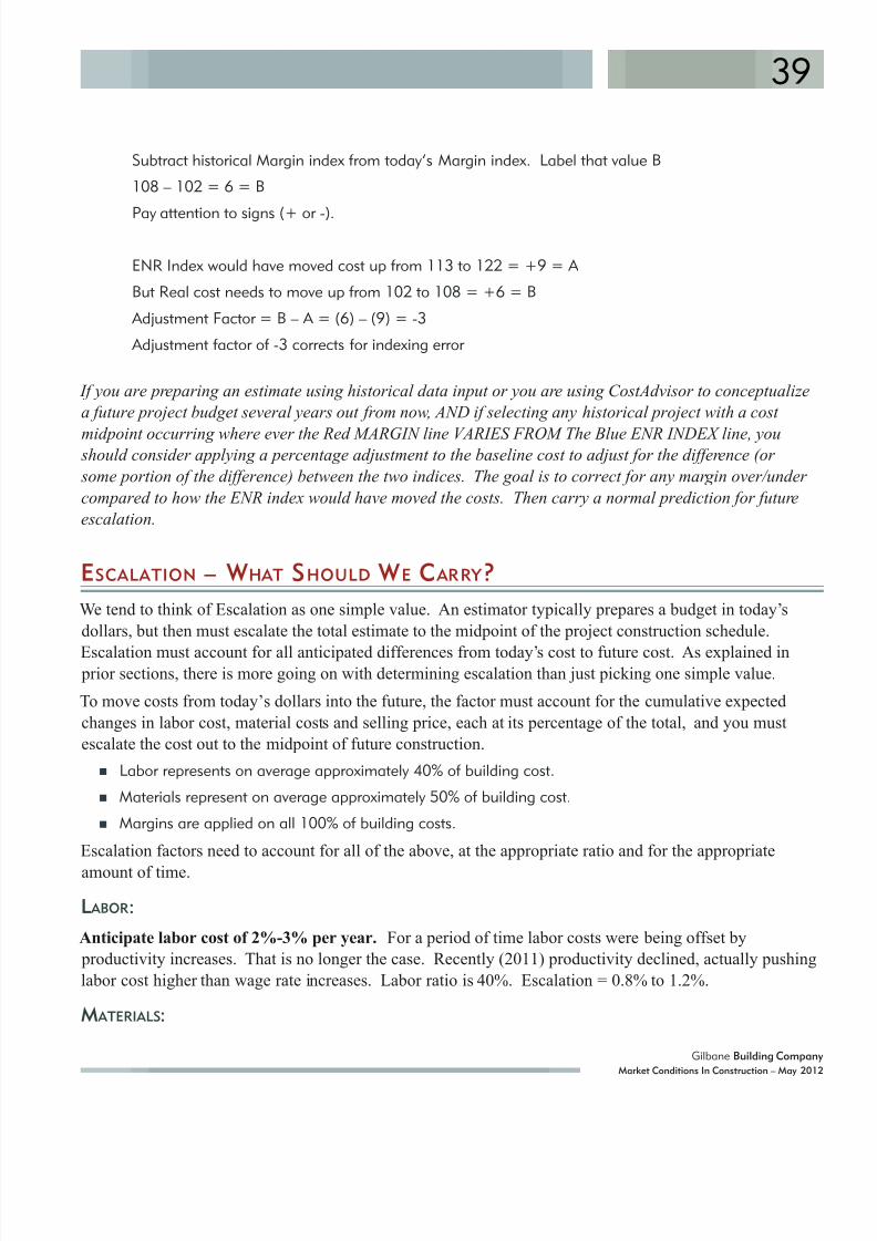
8/10/2019 GBCo Market Conditions Spring 2012
http://slidepdf.com/reader/full/gbco-market-conditions-spring-2012 43/48
39
Gilbane Building Company
Market Conditions In Construction – May 2012
Subtract historical Margin index from today’s Margin index. Label that value B
108 – 102 = 6 = B
Pay attention to signs (+ or -).
ENR Index would have moved cost up from 113 to 122 = +9 = A
But Real cost needs to move up from 102 to 108 = +6 = B
Adjustment Factor = B – A = (6) – (9) = -3
Adjustment factor of -3 corrects for indexing error
If you are preparing an estimate using historical data input or you are using CostAdvisor to conceptualize
a future project budget several years out from now, AND if selecting any historical project with a cost
midpoint occurring where ever the Red MARGIN line VARIES FROM The Blue ENR INDEX line, you should consider applying a percentage adjustment to the baseline cost to adjust for the difference (or
some portion of the difference) between the two indices. The goal is to correct for any margin over/under
compared to how the ENR index would have moved the costs. Then carry a normal prediction for future
escalation.
ESCALATION – WHAT SHOULD WE C ARRY ?
We tend to think of Escalation as one simple value. An estimator typically prepares a budget in today’s
dollars, but then must escalate the total estimate to the midpoint of the project construction schedule.
Escalation must account for all anticipated differences from today’s cost to future cost. As explained in prior sections, there is more going on with determining escalation than just picking one simple value.
To move costs from today’s dollars into the future, the factor must account for the cumulative expected
changes in labor cost, material costs and selling price, each at its percentage of the total, and you must
escalate the cost out to the midpoint of future construction.
Labor represents on average approximately 40% of building cost.
Materials represent on average approximately 50% of building cost.
Margins are applied on all 100% of building costs.
Escalation factors need to account for all of the above, at the appropriate ratio and for the appropriate
amount of time.
L ABOR:
Anticipate labor cost of 2%-3% per year. For a period of time labor costs were being offset by
productivity increases. That is no longer the case. Recently (2011) productivity declined, actually pushing
labor cost higher than wage rate increases. Labor ratio is 40%. Escalation = 0.8% to 1.2%.
M ATERIALS:

8/10/2019 GBCo Market Conditions Spring 2012
http://slidepdf.com/reader/full/gbco-market-conditions-spring-2012 44/48
40
Gilbane Building Company
Market Conditions In Construction – May 2012
Anticipate material costs passed along to only reach 5% to 6%, even though the PPI for construction
materials in 2012 may reach 6%-9%. Material ratio is 50%. Escalation = 2.5% to 3%.
For 2011, PPI for material inputs to non-residential construction increased 5.8%. For that same period totalcosts passed on to the owner were less than 3%, so only half of material cost was reaching the end consumer.
Current economic conditions lead to expectations of ination. However demand, or lack of it, will inuence
the cost of materials. Slow (but steady) growth in spending indicates continued slow demand growth.
Anticipate on average only moderate material price increases. As demand increases, costs passed on will
increase.
M ARGINS:
Anticipate 1% to 1.5%/yr increase to margins unless activity picks up dramatically, then increase rate
of margin growth to 2%/year. Margins are applied on all costs, therefore the ratio is 100%. Escalation =
1% to 2%.
Selling price represents contractor margins and is market activity dependent. Competition will cause project
bid margins to stay low in early 2012 but margins have already been on the increase. Bid costs will show
greater rate of increase before year-end. When we nally see substantial growth in the volume of projects
coming to bid, the need to keep margins reduced will diminish and margins will begin a return to normal.
There is no room left for depressed market activity to move margins lower. Expect margins to increase slowly
over time.
Selling prices are still depressed and it will take time before workload volumes increase to a point that
contractors see a return to normal margins. Nearly 75% of contractors lowered margins in 2010 bids. More
than 75% kept margins the same in 2011 or lowered them even more. Both the New Construction Starts
gures reported by McGraw Hill in the last several months and the March to July 2011 Architectural BillingsIndex published by the AIA are currently proving the delayed increase in construction activity. This should
turn stronger in Q2 2012. The FMI Q1 CIRT Sentiment report indicates 40% of rms anticipate modest
growth in 2012, however the recent AGC March Outlook report indicates only 12% of contractors expect
construction to improve in 2012. It may be several years before the construction workforce and building
markets return to pre-recession levels.
CUMULATIVE COSTS AFFECTING ESCALATION FACTOR:
Labor = 0.8% to 1.2%
Materials = 2.5% to 3%
Margins = 1% to 2%
Potential range of escalation (rounded off) from low of 4% to high of 6%. This could be considered a range
for escalation for the next few years. The 2012 baseline prediction noted here is using the low end of the
range.

8/10/2019 GBCo Market Conditions Spring 2012
http://slidepdf.com/reader/full/gbco-market-conditions-spring-2012 45/48
41
Gilbane Building Company
Market Conditions In Construction – May 2012
TOTAL ESCALATION FOR 2012 = 4% MINIMUM
Assumes slow but continued growth in activity which allows passing along only some labor and material
costs and potentially increasing margins 1%.If construction activity increases rapidly, we would quickly reach the high end of 6%, but unlikely.
I anticipate growth accelerating in the second half and potentially pushing escalation to 5%.
Consider your market. If you are in a market area that has expectations of a huge volume of work that
may start within a narrow window of time, then market pricing can turn rapidly for you. In this specic
condition, it would reasonable to assume 6% annual escalation as a conservative approach in a rapidly
growing market. All labor and material cost will get passed along and margins will increase dramatically.
Let’s not forget that building construction real cost escalation was 8%-10% in 2006 and 7%-8% in 2008.
For 2013
There has been some discussion that immediately following this deationary period we could experience
hyper-ination. Contrary to what some economists think, I have read and share numerous opinions that
construction markets are so deeply depressed it will take more like 2 to 3 years to return to active markets
with normal margins and truly inated labor and material costs. If this does occur, I believe it will not
appear before the end of 2013. I expect there will still be some discount bidding well into next year. But
there is no room left to reduce margins further. Margins will not be reduced as much as they had been.
More of the labor and material cost increases will very likely be passed along.
Potential range of escalation from low of 5% to high of 7%. I believe the potential range of 5% to 6%
escalation may accompany a period of unusual ination in construction. The 2013 baseline prediction noted
here is using the low end of the range.
TOTAL ESCALATION FOR 2013 = 5%
Assumes moderately greater rate of growth in activity which allows passing along most labor andmaterial costs and increasing margins 1% to 1.5%.
If construction activity increases rapidly, we would quickly reach the high end of 7%, but unlikely.
Steady growth greater than anticipated could potentially push escalation to 6%.
TOTAL ESCALATION FOR 2014 = 6%
Assumes greater rate of growth in activity than 2013 which allows passing along all potentially
inflationary labor and material costs and increasing margins 1%-2%.
Looking out to 2014, normal construction activity growth and a path of return to normal margins indicate
we will probably approach the higher end of the escalated cost range. By this time contractors may
potentially increase margins 2%. Inationary pressures may push the rate of material costs increases higher
than the 2%-3% range. All material cost increases from the manufacturer through the supplier may be
passed along. It’s difcult to reach any conclusion that total costs within the year would not be escalated to
at least 6%-7% over the previous year. Any assumption that escalation growth would be less requires that

8/10/2019 GBCo Market Conditions Spring 2012
http://slidepdf.com/reader/full/gbco-market-conditions-spring-2012 46/48
42
Gilbane Building Company
Market Conditions In Construction – May 2012
market activity does not continue to grow and that contractors will not be able to grow margins, even though
still only 60% of the way back from the margins lost since 2006.
Figure 15 Escalation Minimum and Potential
Inflation / Escalation
-9.0%
-6.0%
-3.0%
0.0%
3.0%
6.0%
9.0%
2000 2002 2004 2006 2008 2010 2012 2014
minimum and potential range
The ABI predicts activity 9 to 12 months
out and indicated a slight downturn which
we are currently going through. Indexes
above 50 indicate increasing billings. Since
July 2011, all the ABI market indices have
been climbing. This bodes well for newly
anticipated work growth in Q2-Q3 2012.
8/10/2019 GBCo Market Conditions Spring 2012
http://slidepdf.com/reader/full/gbco-market-conditions-spring-2012 47/48
43
Gilbane Building Company
Market Conditions In Construction – May 2012
Gilbane Inc., is a full service construction and real estate development
company, composed of Gilbane Building Company, Gilbane Development
Company, and ITSI Gilbane. The company (www.gilbaneco. com) is one
of the nation’s largest construction and program managers providing a full
slate of facilities related services for clients in educational, healthcare, life
sciences, mission critical, corporate, sports and recreation, criminal justice,
public and aviation markets. Gilbane has ofces in ten regions of the
country, with corporate ofces located in Providence, Rhode Island. The
information in this report is not specic to any one region.
Author Ed Zarenski is a 40-year construction veteran and a member of the
Gilbane team for more than 30 years. Ed is an Estimating Executive who
has managed multimillion dollar project budgeting, owner capital plan
cost control, value engineering and life cycle cost analysis. He compiles
economic information and provides data analysis and opinion for this
quarterly report.
QUESTIONS REGARDING THIS REPORT CAN BE ADDRESSED TO:
Edward R. Zarenski
Estimating Executive - NENG
Gilbane Building Company
Providence, Rhode Island
8/10/2019 GBCo Market Conditions Spring 2012
http://slidepdf.com/reader/full/gbco-market-conditions-spring-2012 48/48
44
D ATA SOURCES:
Among countless news articles, these sources are used for data in this report
American Institute of Architects – www.aia.org/practicing/economics/index.htmAmerican Iron and Steel Institute - steel.org
American Recycler - americanrecycler.com
Associated Builders and Contractors - abc.org
Associated General Contractors of America - agc.org
Bloomberg L.P. Financial News - Bloomberg.com
Bureau of Labor Statistics - Stats.BLS.gov
Census Bureau - census.gov
Construction Industry Round Table – www.cirt.org
Data Digest – agc.org/datadigest
Economic Cycle Research Institute businesscycle.comEnergy Information Administration - Eia.doe.gov
Engineering News Record - ENR.com
Financial Times - FT.com
Financial Trend Forecaster - Fintrend.com
FMI Management Consulting - FMINET.com
IHS Global Insight - ihs.com
Institute for Supply Management - ism.ws
International Iron and Steel Institute - Worldsteel.org
McGraw Hill – Dodge – construction.com/about-us/press
Metal Miner - agmetalminer.comMetal Prices – metalprices.com
Producer Price Indexes - bls.gov/ppi/
Reed Construction Data - reedconstructiondata.com
RS Means - rsmeans.reedconstructiondata.com
Sageworks – sageworksinc.com
Engineering News Record materials graphics and BCI table reprinted by permission
Financial Trend Forecaster Moore Ination Predictor graph reprinted by permission
U. S. Census Bureau data tables reprinted from public domain
U. S. Bureau of Labor Statistics data tables reprinted from public domainMetalprices material cost data charts from free metalprices.com
All other graphs and tables created by E Zarenski, Gilbane Building Company
Graphs and Tables reprinted by permission may not be reproduced outside this report.