Today’s Agenda

• GPS• Imagery (optical and radar)• Topography

For more info on Remote Sensing, there is a class:Introduction to the Physics of Remote Sensing (EE/Ge 157 abc)

GPS

Our use of GPS:

• Location of surveys O(m)• Topographic corrections for gravity surveys O(cm)• Could make a high res DEM (not needed)

We will use both hand held GPS and RTK GPSRTK = real time kinematic, a form of differential GPS

GPS constellation• 28 GPS satellites

– Designated by PRN (1-33) or SVN/GPS number (currenlty, 1-59)

• Each GPS satellite is in a 26,000 km orbit

• Each satellite broadcasts unique ranging codes and ephemeris information for the entire constellation

• Each satellite has its own response to non-gravitational forces such as solar pressure and commanded maneuvers

• Position in the orbit is known to about 2 cm (eventually)

• Civilian and other uses require only 1-10 meter orbit knowledge

• Scientific users demand much more

What is GPS?

• GPS is a timing system– Clocks– Ranging based on time of flight of signal

from transmitter to receiver– Plus

• Media delays• Instrument delays• Physical models

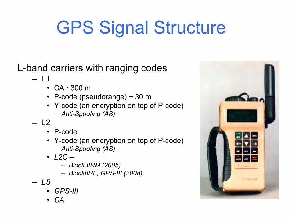
GPS Signal Structure

L-band carriers with ranging codes– L1

• CA ~300 m • P-code (pseudorange) ~ 30 m• Y-code (an encryption on top of P-code)

Anti-Spoofing (AS)– L2

• P-code• Y-code (an encryption on top of P-code)

Anti-Spoofing (AS)• L2C –

– Block IIRM (2005)– BlockIIRF, GPS-III (2008)

– L5• GPS-III• CA

Low Precision Users• Simple receivers

– Track L1– Minimum of 4 satellites tracked– Use ranging code and broadcast

ephemeris to triangulate• Precision limited by

– Orbit error– Clock error

• Selective Availability (SA)– Ranging errors– Propagation delays

• Typical civilian user– Hiker– Automobiles– Etc.

High Precision User• More complex receivers

– Track phase of L1, L2, and ranging codes

– Sophisticated tracking loops– Cross correlated observations for

minimizing Y-code– Track all satellites visible (8-12)– Collect carrier phase, ranging

codes, and broadcast ephemeris• Better antennas

– Multi-path is an issue• Post processing

– Determine position and other parameters using observations and precise ephemeris

GPS Satellite / Orbits / Clocks

APPLICATION: 3-D Crustal MotionTectonic motionOcean tidesSolid earth tidesSubsidenceGlacial isostatic adjustmentMonument stability

PropagationIonosphereTroposphere(wet & dry)

GLOBAL POSITIONING SYSTEM

GPS Receiver• Clocks• Multipath• Antenna phase

center variation

24 Total SatellitesMinimum 4 necessary to correct receiver clock errors

Geometric dilution of precision (GDOP)

CONTINUOUS (PERMANENT) GPS

Give daily/sub-daily positions

Provide significantly more precise data:• No errors in setting up equipment and

reoccupying sites• Stable monuments• More positions to constrain secular rates

Can observe transient signals such as due to earthquake

Early Mobile GPS Technology

JPL’s SERIES Codeless Receiver c. 1981(Satellite Emission Radio Interferometric Earth Surveying)

Remote Sensing

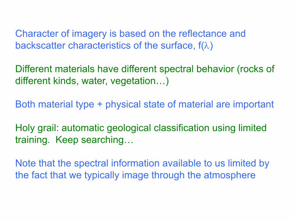
Character of imagery is based on the reflectance and backscatter characteristics of the surface, f(l)

Different materials have different spectral behavior (rocks of different kinds, water, vegetation…)

Both material type + physical state of material are important

Holy grail: automatic geological classification using limited training. Keep searching…

Note that the spectral information available to us limited by the fact that we typically image through the atmosphere

Spectra of common rocks/minerals

Atmospheric absorption

Spectra of common vegetation +

Critical questions to ask when using imagery

1. Spatial resolution (pixel size)2. Image extent (General rule: target is always on the boundary)3. Wavelength4. $$$$

Common systems

Platform Pixel (m) Extent (km) Cost ($)Aster 15/30 60 FREE!!!!!!Landsat 4,5,7 15/30 180 $400+*Landsat 8 5/30 180 FREE!!!!!!Sentinel-2ab 10/60 290 FREE!!!!!! (5 day repeat, 13 bands)SPOT** 5/10 60 O(1000)Ikonos*** 1/4 10 O(1000)Planes/Helicopter O(10cm) 10**** ----

+ Quickbird, Worldview,…

* Perhaps now free** French*** Military**** Camera + height above ground

Landsat:Only 7 spectral bands, not very useful for discerning material types

But because of large image spatial extent and reasonable resolution, good for overview

Instrument VNIR SWIR TIRBands 1-3 4-9 10-14Spatial resolution 15m 30m 90mSwath width 60km 60km 60kmCross track pointing ±318km(± 24°) ±116km(± 8.6°) ±116km(± 8.6°))Quantization (bits) 8 8 12

Note: Band 3 has nadir and backward telescopes for stereo pairs from a single orbit.

ASTER (14 bands)

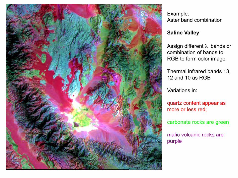
Example:Aster band combination

Saline Valley

Assign different l bands or combination of bands to RGB to form color image

Thermal infrared bands 13, 12 and 10 as RGB

Variations in:

quartz content appear as more or less red;

carbonate rocks are green

mafic volcanic rocks are purple

Sentinel 2 ab

Band number Central wavelength (nm)

Band width (nm) Lref (Wm− 2 sr− 1 μm− 1) SNR @ Lref

1 443 20 129 129

2 490 65 128 154

3 560 35 128 168

4 665 30 108 142

5 705 15 74.5 117

6 740 15 68 89

7 783 20 67 105

8 842 115 103 174

8b 865 20 52.5 72

9 945 20 9 114

10 1380 30 6 50

11 1610 90 4 100

12 2190 180 1.5 100

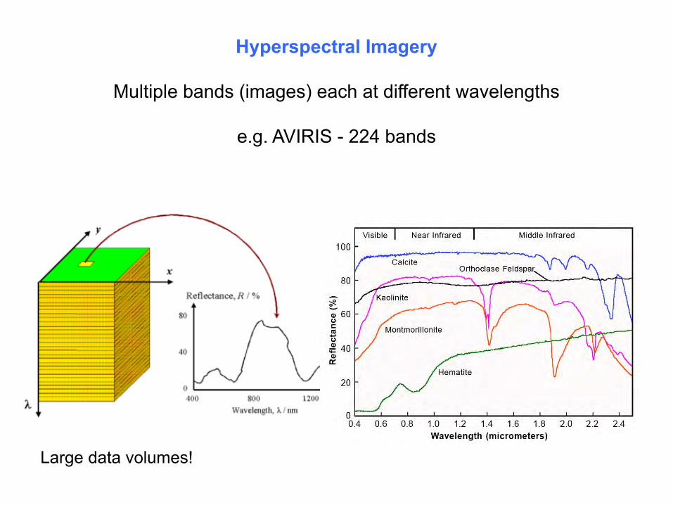
Hyperspectral Imagery

Multiple bands (images) each at different wavelengths

e.g. AVIRIS - 224 bands

Large data volumes!

At radar wavelengths, the atmosphere is transparent

Frequencies and Wavelength of the IEEE Radar Band designation

Band Frequency (GHz) Wavelength (cm)L 1-2 30-15S 2-4 15-7.5C 4-8 7.5-3.75X 8-12 3.75-2.50Ku 12-18 2.5-1.67K 18-27 1.67-1.11Ka 27-40 1.11-0.075

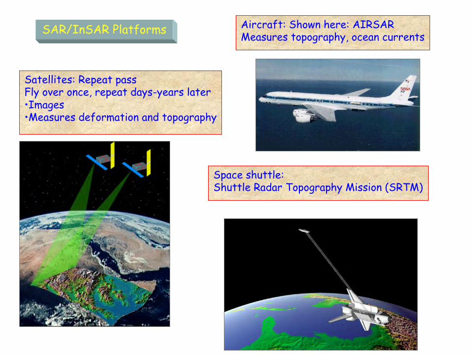
SAR/InSAR Platforms

Both from: JPLFrom: H. Zebker

Satellites: Repeat passFly over once, repeat days-years later•Images•Measures deformation and topography

Space shuttle:Shuttle Radar Topography Mission (SRTM)

Aircraft: Shown here: AIRSARMeasures topography, ocean currents

Radar is active imaging

Natural image coordinates are in units of time: along track (azimuth direction) & line-of-sight (LOS) (range direction)

• foreshortening

• layover

• shadows

Imaging radar is side looking (why?)

Achieve resolution by clever combination of consecutive radar images: Synthetic Aperture Radar (SAR)

Mapping timeàspace

Methods

•Land surveys (now GPS)•Radar altimeter•Air or space borne laser (LIDAR) - point or swath mapping altimeter•Stereo imagery (air photos, now satellite)•Radar interferometry a.k.a. InSAR (plane, shuttle, satellite)

Practical availability

•U.S.: 10-30 m/px (USGS, SRTM) on the net0.5-15 m (Airborne InSAR, optical, LIDAR) - e.g., TOPSAR

•Foreign: 90 m/px (SRTM 60S-60N), 30-60 m/px by begging (classified)900 m/px open access

•Make your own (InSAR, optical) 1-20 m/px

Topography (DEM, DTM, DTED, topo, height,…)

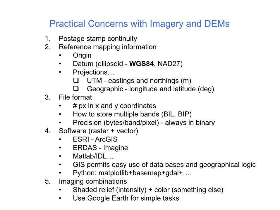
Practical Concerns with Imagery and DEMs1. Postage stamp continuity2. Reference mapping information

• Origin• Datum (ellipsoid - WGS84, NAD27)• Projections…

q UTM - eastings and northings (m)q Geographic - longitude and latitude (deg)

3. File format• # px in x and y coordinates• How to store multiple bands (BIL, BIP)• Precision (bytes/band/pixel) - always in binary

4. Software (raster + vector)• ESRI - ArcGIS• ERDAS - Imagine• Matlab/IDL…• GIS permits easy use of data bases and geographical logic• Python: matplotlib+basemap+gdal+….

5. Imaging combinations• Shaded relief (intensity) + color (something else)• Use Google Earth for simple tasks

What is shaded relief?

Directional gradient mapped to grey scale

Cajon Pass I-15 Fault Crossing

Getting LIDAR data• http://www.opentopography.org/• Get an account• Click on data – select with map• Choose B4 and/or Dragons Back (what’s the difference?)• Select point cloud and have it make the DEM. You probably

want shaded relief KMZ as well as geotiff/img for ARC.• May need to download in overlapping tiles because of file size

limits and odd shape of target area• Submit and wait for email

GIS Homework (due in 2 weeks!)Construct basemaps of the Carrizo Plain region. Your map should be annotated with any geologically interesting features (faults, major geomorphic structures, place names, roads etc.) and include scale bars and geographic reference (ticks or something) as well as legends for any colors or symbols that you use. All annotations should be useful (choose units appropriately) and legible.

Your basemap(s) can use any useful combination of DEMs and imagery. Feel free to experiment! Make it clear what imagery you are using and how you chose your colors.

You will use these maps in 111b to orient yourself in the field, to document where we went, and even possibly to do some geology…

Feel free to use the GIS lab on the 3rd floor of South Mudd as much as you need for this assignment. Lisa Christensen, the Lab manager, will provide an overview on the use of ARC GIS if you have not used it before.

Extract and plot a 1-km-long topographic profile perpendicular to the SAF near our proposed field area. Make sure the profile is nicely annotated. Show the location of the profile on your map.

Measure offset features along the fault. Is there any obvious pattern? Indicate which features you are measuring on one of your maps.