Geant4 simulations of neutron flux using automatedweight windows with applications to ESS

John Stenander

Spring 2015Master’s thesis

Department of PhysicsDivision of Nuclear Physics

Supervisor: Douglas Di JulioCo-supervisor: Joakim Cederkall

Abstract

This thesis investigates the use of two automated weight window methods forvariance reduction of flux in particle transport simulations. The methods are im-plemented in the Geant4 simulation software. Both methods are based on pre-simulations, using flux or relative error information as input. The methods areintended for use in shielding and instrumental background applications and aretested on flux and spectrum calculations using two versions of an European Spalla-tion Source (ESS) instrument shielding target model. For each model, the methodswere implemented by defining a parallel geometry mesh grid which overlaid themass geometry. In each mesh cell the number of tracks in the cell and the relativeerror of the number of tracks were scored. This information was used to update theweight windows.

Two figures of merit were introduced to assess the methods. The first figure ofmerit is inversely proportional to the square of the relative errors and the simu-lation time. The second figure of merit is the standard deviation of the relativeerrors. Both figures of merit showed improvement for the two methods and almostall simulation times. Compared to the analog simulation, the first figure of meritincreased by a factor of 2.17 to 3.10 when applying the relative error based methodand by a factor ranging from 2.10 to 14.60 when applying the flux based method.The second figure of merit decreased by a factor ranging from 1.33 to 2.89 when ap-plying the relative error based method and increased by a factor ranging from 1.58to 3.15 when applying the flux based method. The improvement depends on thesimulation time and the simulated model. The methods showed improved figuresof merit, reduced the parts of the simulated geometry that saw few Monte Carloparticles and reduced the error significantly in almost all spatial regions.

i

Contents

Contents ii

Acknowledgements iii

List of Abbreviations iv

1 Introduction 11.1 General overview . . . . . . . . . . . . . . . . . . . . . . . . . . . . . . . . 11.2 Aim and limitations . . . . . . . . . . . . . . . . . . . . . . . . . . . . . . . 11.3 ESS . . . . . . . . . . . . . . . . . . . . . . . . . . . . . . . . . . . . . . . 21.4 Monte Carlo particle transport simulation software . . . . . . . . . . . . . 21.5 Applications . . . . . . . . . . . . . . . . . . . . . . . . . . . . . . . . . . . 3

1.5.1 Instrument backgrounds . . . . . . . . . . . . . . . . . . . . . . . . 31.5.2 Medical isotopes . . . . . . . . . . . . . . . . . . . . . . . . . . . . 3

2 Theory and background 42.1 Physics overview . . . . . . . . . . . . . . . . . . . . . . . . . . . . . . . . 4

2.1.1 General neutron physics . . . . . . . . . . . . . . . . . . . . . . . . 42.1.2 Spallation physics . . . . . . . . . . . . . . . . . . . . . . . . . . . . 52.1.3 Moderators . . . . . . . . . . . . . . . . . . . . . . . . . . . . . . . 72.1.4 Background & shielding . . . . . . . . . . . . . . . . . . . . . . . . 8

2.2 Monte Carlo methods . . . . . . . . . . . . . . . . . . . . . . . . . . . . . . 102.2.1 Overview of Monte Carlo methods . . . . . . . . . . . . . . . . . . 102.2.2 Error calculation in Monte Carlo methods . . . . . . . . . . . . . . 10

2.3 Variance reduction methods . . . . . . . . . . . . . . . . . . . . . . . . . . 112.3.1 Importance sampling . . . . . . . . . . . . . . . . . . . . . . . . . . 122.3.2 Weight windows . . . . . . . . . . . . . . . . . . . . . . . . . . . . . 122.3.3 Some particular weight window generator methods . . . . . . . . . 142.3.4 An easy to implement global variance reduction procedure . . . . . 16

3 Simulation analysis 173.1 Realization of the method in Geant4 . . . . . . . . . . . . . . . . . . . . . 173.2 Results . . . . . . . . . . . . . . . . . . . . . . . . . . . . . . . . . . . . . . 23

4 Conclusion 314.1 Conclusion . . . . . . . . . . . . . . . . . . . . . . . . . . . . . . . . . . . . 314.2 Outlook and further work . . . . . . . . . . . . . . . . . . . . . . . . . . . 31

References 32

ii

Acknowledgements

I would like to thank my supervisor, Douglas Di Julio, for providing great support duringthe work with the thesis and always pushing me forward. He has been most helpful duringall stages of work and has given me ample opportunities to find an audience for my work.Furthermore, I would like to thank ESS for providing funding for me during the projectand also for giving me a hospitable working environment. A thank you also to JoakimCederkall, for giving me this opportunity and providing comments on the thesis towardsthe end of the work.

iii

List of Abbreviations

ADS - Accelerator Driven SystemCERN - Conseil Europeen pour la Recherche NucleaireESS - European Spallation SourceESS TDR - ESS Technical Design ReportFLUKA - FLUktuierende KAskadeFOM - Figure Of MeritFW-CADIS - Forward Weighted-Consistent Adjoint Driven Importance SamplingGeant4 - GEometry ANd TrackingGFWW - Global Flux Weight WindowsGRWW - Global Response Weight WindowsGVR - Global Variance ReductionHP - High Precision neutron modeli.i.d. - Independent and Identically DistributedINC - Intra-Nuclear CascadeLVR - Local Variance ReductionMCNP - Monte Carlo N-Particle Transport CodePDF - Probability Density FunctionPHITS - Particle and Heavy Ion Transport code SystemTS - Thermal ScatteringS/N - Signal to noise ratioQGSP - Quark-Gluon String Precompound

iv

1 Introduction

1.1 General overview

Monte Carlo simulation (section 1.4) is a great tool to use in many of the quantitativesciences, ranging from economics to biology and of course physics. These simulations arecomputationally intensive and there is a need to work with complex systems and problemsin an efficient way. This thesis will provide a method for efficient computer simulationsfor use in neutron transport problems in spallation source applications.

A computer can only handle just so many particles thus a simulation will inevitablywork with less particles than a real life experiment. Such a simulation may not catch allrare events, and it will produce unreliable statistics for spatial or energy regions that showlow or non-existent particle flux. This problem can in principle be solved by increasingthe simulation time, but it is often so that the values which initially have a good precisionare the ones that gain from this, while the values that need precision improvement do notgain as much. The methods presented in this thesis will provide a way to allocate com-puter resources more efficiently (section 2.3). In a complex simulation there is a tangibleprobability that this poses a real problem. The complex model that is the subject of thisthesis is the ESS target model1. This model was constructed previous to this work inGeant4 [1], a particle transport simulation toolkit. The method that is used is a weightwindow method with windows set using flux and the relative errors of the flux as a basis[2] for the simulation bias.

This thesis will begin with an introduction to the tools of science it will consider, in-cluding both the ESS facility and the simulation software available. Furthermore, anintroduction to the physics of the problem, spallation sources and background radiationwill be given a brief overview as well as Monte Carlo methods in general and a more indepth discussion about variance reduction techniques. The results are presented in thefinal section where it is shown that this method does work as an efficient simulation bias toproduce reliable statistics everywhere without with reduced simulation times. The meth-ods are compared using figures of merit and data for calculated fluxes and the relativeerrors are presented.

1.2 Aim and limitations

The goal of this work is to present a usable non-deterministic weight window (section2.3.2) method to be used in calculations of neutron flux in Geant4. Furthermore, someapplications of this as well as the physics behind spallation (section 2.1.2) sources areexplored.

The model to be used is fixed and so is the implementing platform. While no alterna-tives are considered for use, other methods are described and reviewed in this thesis. Allapplications considered will be taken using the ESS target model (in different forms). Amethod like this would have applications in many different particle transport simulations,

1The ESS target model here and here after refer to the ESS target model for instrument shielding,constructed in Geant4.

1

but only this model is considered in this thesis.

1.3 ESS

ESS is a neutron production facility being constructed in Lund and it is expected to beoperational in 2019. ESS will be the world’s most powerful and modern spallation neutronsource when it reaches full capacity in 2025 [3].

The ESS facility will be a pulsed neutron spallation source with 125 MW peak power[4]. In general, spallation is a process where neutrons are released from a material as aresult of bombardment with medium energy range particles (section 2.1.1). In the partic-ular case of ESS, protons are used with a tungsten target [5].

The primary use of the facility will be the possibility to probe into condensed matterobjects [3]. This is one of the largest research fields of physics as everything around us ismade of condensed matter and the study of it has given us everything from cell phonesto sturdy materials as well as a deeper insight into the structure of the universe. ESSwill act as a large scale powerful microscope, but instead of using photons (light) as theprobing particle, neutrons are to be used. Besides working as an effective microscope itwill provide ways to probe matter in a non-intrusive way. This is useful, for example, tostudy old paintings or running engines [3]. Furthermore, it will be possible to conductfundamental physics experiments at ESS [3].

The ESS facility will be of use for physicists, medical scientists, chemists and archae-ologists amongst others. ESS will also aid the study and improvement of drugs, electroniccomponents and new materials. It will give new ways to investigate historical artifactsand the properties of space.

1.4 Monte Carlo particle transport simulation software

There are many software solutions available for particle transport simulations. The frame-work being used for this project is Geant4, an open source CERN developed package [1].It is important to make it possible for scientists to communicate ideas and to build upontheir peers work. A closed source code makes this harder. Having these models available inGeant4 (or any other open source code) is important for the scientific community in large.

MCNP is another popular software for radiation transport and is available under propri-etary license [6]. The methods that are being used in this project have been implementedusing MCNP [2] and the challenge is to do the same in Geant4.

Geant4 is mainly used for high energy physics simulations while MCNP is developedfor nuclear science problems. Both contain weight window algorithms (section 2.3.2) andwhat is missing in Geant4 is the method to set the weights.

Apart from the two code packages discussed above, one must also mention FLUKA [7]and PHITS [8]. FLUKA is - like the ones mentioned above - a tool for calculations regard-ing particle transport. FLUKA is distributed in binaries but the source code is available

2

under license agreement. PHITS is a Fortran based general purpose particle transportcode and it is distributed as source packages.

While the proximate cause to use Geant4 in this thesis is that the ESS target modelis already implemented and is used among scientists working in the ESS project, thereis a more interesting ultimate cause. Geant4 is written in a modern language (C++), isopen-source and may be modified, it is available freely in source format and is supportedand tested on a number of platforms.

1.5 Applications

1.5.1 Instrument backgrounds

In a spallation source, higher neutron energies than those in a traditional nuclear reac-tor are observed. These can be in the GeV range, compared to ≈ 20 MeV for reactorsources. Shielding is used to lower the background, that would otherwise be detectedby instruments and provide a noise for all measurements. Different shielding materialshave different properties (2.1.4), differing in for example transparency, price and effi-ciency for different types of radiation. Thus, for design purposes, it is important to beable to evaluate the different shielding options. For higher energies, there is still room forimprovements in calculations regarding shielding material properties [9]. The paper byCherkashyna et al. [9] has made tentative Geant4 simulations of some possible shieldingmaterials.

For a spallation source, shielding is important to reduce the high energy backgroundon instruments. Cherkashyna et al. states that shielding may be the best way to re-duce backgrounds. High energy backgrounds have an adverse effect on the S/N (signal tonoise) ratio in instruments and reduce the functionality of the neutron scattering instru-ments. The contributions to the background can arise from deep penetration of neutrons,sky- or groundshine (neutrons scattered from the atmosphere or ground) and streamingalong neutron guides (background radiation that follows neutron guides in the shielding).These are all computationally expensive and warrant a method to perform faster fluxcalculations. For further investigation of these shielding materials in large scale models,a method like the one in this thesis would improve the results.

1.5.2 Medical isotopes

While the primary use of ESS will be neutron scattering experiments, some alternativeuses might be considered. One of these uses is the production of medical radioisotopes.There are many different isotopes in use that are possible for production at ESS and oneof the more interesting is technetium-99m (99mTc). This is a short-lived metastable (hencethe m) isomer of technetium-99 (99Tc). 99mTc is produced by the reaction 99Mo→99m Tc[10]. This can be, and is, produced in nuclear reactors by neutron irradiation of 235U and98Mo. This has some drawbacks. First of all it produces nuclear waste. Second, thereis a predicted shortage and even an almost complete halt in production, as observed bythe trend in historical production, with previous dips in production to set an example [11].

If production of medical isotopes is to be possible, the neutron spectrum has to be known

3

at certain places. A variance reduction method would be of good use to populate thoseregions properly.

2 Theory and background

2.1 Physics overview

2.1.1 General neutron physics

In this chapter - and further physics sections - some aspects of neutron physics are dis-cussed. For this an outline of neutron naming conventions and categorization is needed.Neutrons are categorized and named based on their energy ranges. This nomenclaturewill be used in this thesis and is summarized in table 1.

Table 1: Used neutron naming conventions [12].

Energy range NameUp to 0.025 eV Cold neutronsAround 0.025 eV Thermal neutrons1 to 10 eV Slow neutrons1 to 20 MeV Fast neutrons> 20 MeV Relativistic neutrons

Neutron transport is governed by the neutron transport equation [13]. The solution andapplications of this equation are not considered here as this work will implement a non-deterministic Monte Carlo method.

Two important concepts in neutron physics are the cross section and the mean freepath. The cross section (σ) is a factor measured in the unit of barn, 1 b = 10−24 cm2.The cross section characterizes the probability that a given reaction occurs. The macro-scopic cross section (Σ) is the cross section of a nuclide times the number of atoms percm3. The macroscopic cross section (Σ) can be defined as Nσ = Σ where N is the den-sity of nuclei and thus gives the probability for reaction per travelled distance (cm−1) [14].

Related to cross sections is the mean free path (λ). Take p(x) as the probability that aneutron has not had a reaction while traveling the distance x in a homogeneous medium.It follows that

dp = Σpdx⇔ p(x) = e−Σx ⇒ dp

dx= Σe−Σx, (1)

which is the probability of a reaction when a neutron travels over the distance dx. Theexpected value of x is called the mean free path and given as

λ =

∫ ∞0

= xΣe−Σxdx =1

Σ, (2)

where λ is a measure of how far we expect a neutron to travel before a reaction [13].

4

2.1.2 Spallation physics

A theory of spallation

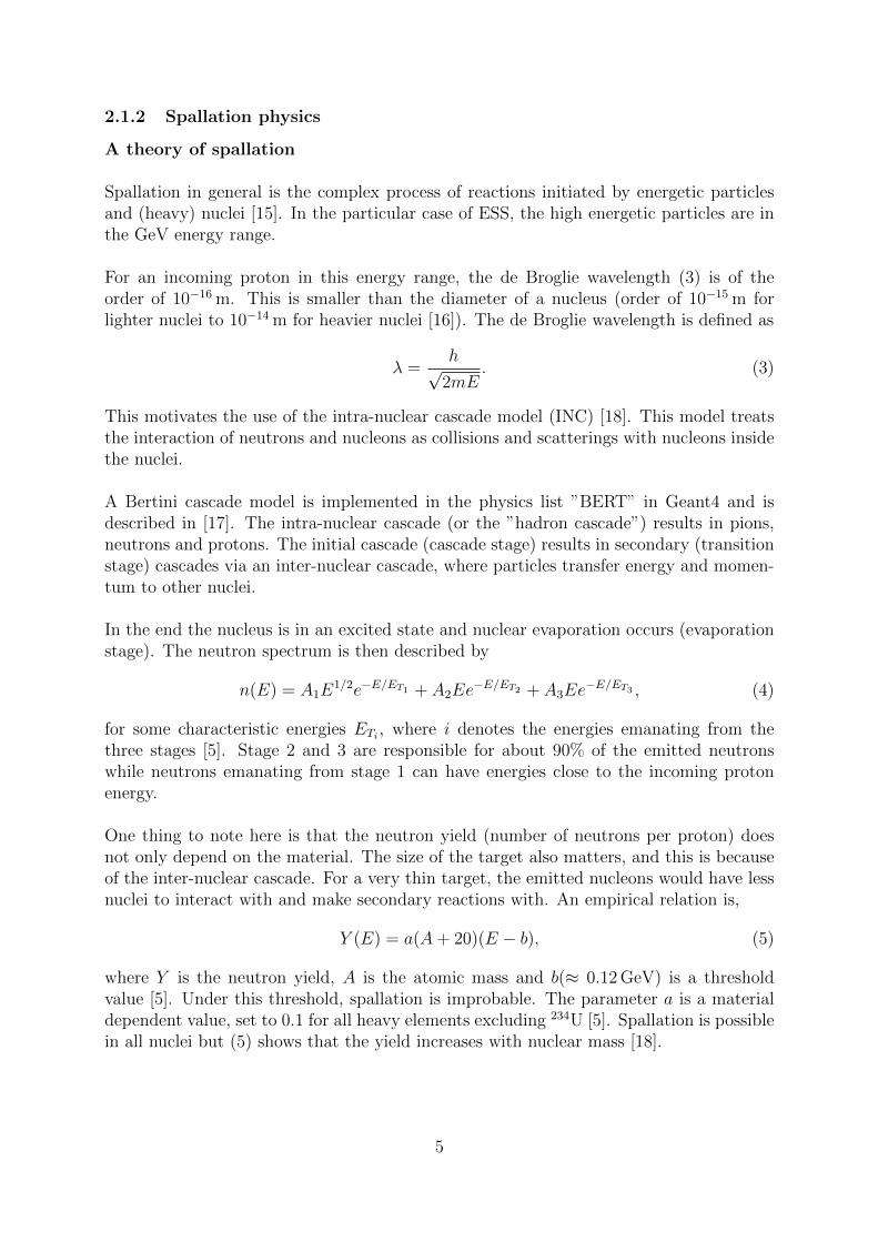
Spallation in general is the complex process of reactions initiated by energetic particlesand (heavy) nuclei [15]. In the particular case of ESS, the high energetic particles are inthe GeV energy range.

For an incoming proton in this energy range, the de Broglie wavelength (3) is of theorder of 10−16 m. This is smaller than the diameter of a nucleus (order of 10−15 m forlighter nuclei to 10−14 m for heavier nuclei [16]). The de Broglie wavelength is defined as

λ =h√

2mE. (3)

This motivates the use of the intra-nuclear cascade model (INC) [18]. This model treatsthe interaction of neutrons and nucleons as collisions and scatterings with nucleons insidethe nuclei.

A Bertini cascade model is implemented in the physics list ”BERT” in Geant4 and isdescribed in [17]. The intra-nuclear cascade (or the ”hadron cascade”) results in pions,neutrons and protons. The initial cascade (cascade stage) results in secondary (transitionstage) cascades via an inter-nuclear cascade, where particles transfer energy and momen-tum to other nuclei.

In the end the nucleus is in an excited state and nuclear evaporation occurs (evaporationstage). The neutron spectrum is then described by

n(E) = A1E1/2e−E/ET1 + A2Ee

−E/ET2 + A3Ee−E/ET3 , (4)

for some characteristic energies ETi , where i denotes the energies emanating from thethree stages [5]. Stage 2 and 3 are responsible for about 90% of the emitted neutronswhile neutrons emanating from stage 1 can have energies close to the incoming protonenergy.

One thing to note here is that the neutron yield (number of neutrons per proton) doesnot only depend on the material. The size of the target also matters, and this is becauseof the inter-nuclear cascade. For a very thin target, the emitted nucleons would have lessnuclei to interact with and make secondary reactions with. An empirical relation is,

Y (E) = a(A+ 20)(E − b), (5)

where Y is the neutron yield, A is the atomic mass and b(≈ 0.12 GeV) is a thresholdvalue [5]. Under this threshold, spallation is improbable. The parameter a is a materialdependent value, set to 0.1 for all heavy elements excluding 234U [5]. Spallation is possiblein all nuclei but (5) shows that the yield increases with nuclear mass [18].

5

Spallation in practice

Spallation is one method to release neutrons. There are other sources for neutron emissionwith the most common man-made sources using fission and fusion. There are still othernatural occurring sources stemming from spontaneous fission or radioactive decay [19].Unlike the two other methods - fission and fusion - spallation is endothermal and doesnot currently find any direct use in the energy industry (but it would be possible to use aspallation source to drive a fission reactor, such a solution is called an accelerator drivensystem (ADS) [20]).

Spallation reactions are induced and maintained with an energetic beam. At ESS a 2 GeVproton beam will be used [3]. Furthermore, spallation sources generate a hard neutronspectrum (high neutron population at higher energies). See Figure 1 for a comparisonbetween a fission neutron spectrum and a spallation neutron spectrum generated usingan 800 MeV proton beam [5]. The neutron yield is ≈ 20 in practical applications [15] andcan be calculated using (5).

So far, the described spallation source consists of two components, a proton source and atarget (tungsten in the ESS case [3]). Further components include the moderators, shields,beam tubes and reflectors. The moderators and shielding will be discussed in some detailin sections 2.1.3 and 2.1.4. An outline of the ESS target target region is shown in Figure2.

Figure 1: Calculated fission (◦) and spallation (·) neutron spectra [5]2.

2Reprinted from Nuclear instruments & methods in physics research, 463(3):505-543, G.S. Bauer,Physics and technology of spallation neutron sources, 39., 2001, with permission from Elsevier.

6

Figure 2: Outline of the ESS target region based on figures in Ref. [3]. In this figurethe most important components are shown. The components that are discussed in thefollowing sections in particular are the moderators, shielding and reflectors.

2.1.3 Moderators

In neutron scattering experiments, mainly neutrons in the cold or thermal ranges areuseful (that is in the meV to eV range). Neutrons from a spallation reaction can be in thefast or even relativistic ranges [18]. This gives rise to the need of moderation as well asmoderation with other characteristics than those in fission reactors. The primary purposeof the moderator is to lower the velocity of high energy neutrons and place them in athermal or cold spectrum. For scattering experiments, long wave-length or cold neutronsare preferred.

Furthermore, the primary beam at ESS as well as in similar constructions, is pulsed.This puts an extra demand on the moderator as it has to preserve the time structure andneutron brightness. For this reason, moderators designed for spallation sources will besmaller than their counterparts in fission reactors. The energy loss of neutrons are due toelastic scattering (collisions without excitation) with the moderator nuclei [13, 21].

Another factor is how often these collisions occur, which is dependent on the mean freepath (see section 2.1.1). If the energy loss per collision and expected number of collisionsper traveled distance is known then it is possible to calculate the total energy loss fora certain volume of the medium. The mean free path is inversely proportional to thescattering cross section, hence a large value for Σ is desired to give a small mean free path[5].

The fraction of energy lost in each collision is constant (E1

E2= const.) and the logarithm

of this is given by

ζ = lnE1 − lnE2 = 1− (α0ε

1− α0ε), (6)

using ε = ln( 1α0

) and α0 = (A−1)2

(A+1)2and atomic number A [5]. ζ is one for A = 1 and

decreases with A, making hydrogen the most efficient moderator element.

To make the loss independent of initial energy it is useful to adopt another scale forenergy. Let u = ln E0

Ewith E0 = 10 MeV, chosen so that u > 0 for most relevant neu-

7

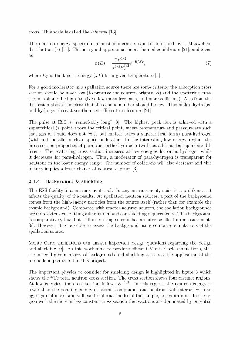
trons. This scale is called the lethargy [13].

The neutron energy spectrum in most moderators can be described by a Maxwelliandistribution (7) [15]. This is a good approximation at thermal equilibrium [21], and givenas

n(E) =2E1/2

π1/2E3/2T

e−E/ET , (7)

where ET is the kinetic energy (kT ) for a given temperature [5].

For a good moderator in a spallation source there are some criteria; the absorption crosssection should be made low (to preserve the neutron brightness) and the scattering crosssections should be high (to give a low mean free path, and more collisions). Also from thediscussion above it is clear that the atomic number should be low. This makes hydrogenand hydrogen derivatives the most efficient moderators [21].

The pulse at ESS is ”remarkably long” [3]. The highest peak flux is achieved with asupercritical (a point above the critical point, where temperature and pressure are suchthat gas or liquid does not exist but matter takes a supercritical form) para-hydrogen(with anti-parallel nuclear spin) moderator. In the interesting low energy region, thecross section properties of para- and ortho-hydrogen (with parallel nuclear spin) are dif-ferent. The scattering cross section increases at low energies for ortho-hydrogen whileit decreases for para-hydrogen. Thus, a moderator of para-hydrogen is transparent forneutrons in the lower energy range. The number of collisions will also decrease and thisin turn implies a lower chance of neutron capture [3].

2.1.4 Background & shielding

The ESS facility is a measurement tool. In any measurement, noise is a problem as itaffects the quality of the results. At spallation neutron sources, a part of the backgroundcomes from the high-energy particles from the source itself (rather than for example thecosmic background). Compared with reactor neutron sources, the spallation backgroundsare more extensive, putting different demands on shielding requirements. This backgroundis comparatively low, but still interesting since it has an adverse effect on measurements[9]. However, it is possible to assess the background using computer simulations of thespallation source.

Monte Carlo simulations can answer important design questions regarding the designand shielding [9]. As this work aims to produce efficient Monte Carlo simulations, thissection will give a review of backgrounds and shielding as a possible application of themethods implemented in this project.

The important physics to consider for shielding design is highlighted in figure 3 whichshows the 56Fe total neutron cross section. The cross section shows four distinct regions.At low energies, the cross section follows E−1/2. In this region, the neutron energy islower than the bonding energy of atomic compounds and neutrons will interact with anaggregate of nuclei and will excite internal modes of the sample, i.e. vibrations. In the re-gion with the more or less constant cross section the reactions are dominated by potential

8

Figure 3: Total neutron reaction cross sec-tion for 56Fe [25]

Figure 4: Total neutron reaction cross sec-tion for 1H [25]

scattering and the cross section is more or less the geometric cross section of the nuclei.The spiked region is because of the resonance structure and can be described by (8). Inthe highest energy region the cross section drops off, this follows the energy dependentwavelength drop (3). The reaction probability will decrease with this wavelength [22].

Of particular importance are materials, like mild-steel for example, which show a pro-nounced resonance structure for given neutron frequencies [23]. These show up as thepeaks in the cross section, as discussed above for Figure 3. This can be compared withhydrogen (Figure 4) which does not exhibit a resonance structure for any energy ranges.The peak is described by the Breit-Wigner formula [23], as E → 0, given by

σn,γ(E) ≈ π(λ

2π)2 ΓnΓγ

E2R

. (8)

This formula gives a good predictive relation between cross section and the neutron en-ergy, where λ is the de Broglie wavelength, Γn/γ ∝ 1

τis the resonance width and ER

is the resonance energy. The resonance discussed here is a metastable state formed byan incoming particle. In general a resonance is defined as a short-lived particle state.The dips in the cross section are a result of interference between potential and resonancescattering. A mathematical despription of this (see Ref. [23]) involves three terms, onedescribing potential scattering, one describing resonance scattering and one describingthe interference. With E < ER the last term is negative, thus showing destructive in-terference. This destructive interference give rise to the dips in the cross section. A lowcross section implies a long mean free path, that is neutrons travel longer distances beforereacting with the shielding material.

For neutron scattering there are four primary materials to use as shielding.

� Concrete - A cheap hydrogen containing material. Used to shield high energyphotons and to moderate fast neutrons.

� Steel - A cheap material. Used to stop fast neutrons. Some steels show neutrontransparency for some energy ranges.

� Plastic - Slow fast neutrons, i.e. moderation.

9

� Boron-containing substance - A material to capture slow and thermal neutrons.

All of these materials have relevant cross section properties for neutron shielding. How-ever, they may not be ideal for other types of radiation, such as photons. Often a com-bination of the materials is useful when constructing shielding for neutron sources. Ko-privnikar and Schachinger [24] have studied multi-layered and sandwich designs for theESS and stressed the need of Monte Carlo simulations with variance reduction (section2.3).

2.2 Monte Carlo methods

2.2.1 Overview of Monte Carlo methods

The name Monte Carlo is given to members of a class of simulation techniques that utilizerepeated and random sampling to achieve the convergence to a true distribution. This canbe contrasted to traditional methods that use ”abstract thinking” [26] that often resultin a neat closed form expression that can give the answer to what will happen in a sys-tem under all circumstances. The prime example here would be Newton’s laws of motionbut even these laws will have problems making predictions already with three bodies. Inparticle transport problems, the real problem would have to consider millions of particles(or more). This stresses the need of a Monte Carlo method, a method to take randomsamples of particles to make predictions.

One of the questions considered in this thesis is how to take the samples. It mightbe that the analog simulation - the direct simulation of real physical events - is the best[27]. Another possibility is to sample different geometrical regions more or less. In theanalog simulation, particles would be produced with a uniform weight of one and unevenlyspread over the geometry of the simulation. In a biased simulation one goal may be tospread particles evenly over the simulated geometry. Of course it is impossible to find amethod to make the geometrical spread of particles perfect, but this thesis is concernedwith the problem of finding a good spread.

In a computer simulation, one would either want some specific tallies (measurementsover the mesh grid) or a good distribution with low relative errors over the entire grid[28]. In this thesis both cases will be considered but the method presented is best suitedfor the latter case.

2.2.2 Error calculation in Monte Carlo methods

In all statistical models and simulations of physical processes the error is an importantcharacteristic. The error quantifies the uncertainty of an experiment, measurement orsimulation. The uncertainties in a Monte Carlo simulation arise not from instrumentaldifficulties but only from a limited sampling process. In this thesis, the relative error isused to quantify the end result and to compare the quality of simulation runs and also asa basis to set the weight windows.

The error is given by (9) for a random variable X with measurements i. Assuming a

10

normal distributed variable, the error in a given mesh cell is given by

error =σ√N, (9)

where

σ =

√√√√ 1

N(N∑i=1

X2i −

1

N(N∑i=1

Xi)2). (10)

The relative error is the error relative to the the variable X itself, as in

Re =error

X∝ 1√

N. (11)

The relative error will decrease with the square of N , i.e. the number of measurements.This means that the more events, the lower the relative error will be. This measure is notto be confused with the accuracy of the simulation. It is possible to be off the mark by alarge distance, for example if the model is faulty or completely wrong, while still havinga low error. A low error only refers to the precision in the Monte Carlo simulation [29].A guideline to interpreting the relative errors can be found in table 2.

Table 2: Guidlines for interpreting relative error [29].

Range of Re Quality0.5 to 1 Not meaningful0.2 to 0.5 Factor of a few0.1 to 0.2 Questionable<0.1 Generally meaningful

2.3 Variance reduction methods

This thesis will consider the weight window method which is a member of a broader classof variance reduction methods. These methods can be divided in two; local variance re-duction (LVR) or global variance reduction (GVR). This thesis will consider GVR, wherethe task is to reduce the variance in all parts of a geometry. These are methods used withMonte Carlo simulations in physics to increase computational efficiency. The aim of GVRis to transport particles everywhere in a model, to catch as many events as possible and togive statistically relevant data everywhere. This has to be done while being conservativewith computational power [2, 30].

The general idea will be to weight particles according to some rule. In real life or inthe analog simulation all particles will be weighed as one. With a GVR method particleswill have a weight ≤ 1. A GVR method lets events happen in a spatial-energy regionwhere they would otherwise be non-existent or rare with a computationally feasible analogrun. The question now is how to find a method to weight particles in proper ways to letthem propagate through the model without sacrificing computational time.

11

This section gives an overview of importance sampling, as well as the weight windowmethod itself along with a review of some common methods to set weight windows. Oneof the methods, Van Wijk’s method [2] is used in all simulations carried out in this work.

2.3.1 Importance sampling

While this thesis will concentrate on the weight window method, importance sampling isthe most commonly used method for simulation of rare events. Instead of sampling thedirect distribution (p(·)), to estimate the expected value of f(X) for the random variableX, the sample is taken from

E[f(X)] =1

k

k∑i=1

f(Yi)p(Yi)

q(Yi), (12)

where p(·) is the PDF for X, q(·) is the importance distribution, Y are i.i.d. (independentand identically distributed) random numbers and k is the number of sampling points [31].(12) is an unbiased estimate of the expected value of X3.

It is reasonable to ask why this is useful. Different choices of q(·) result in differentvariances. There is an optimal choice of q(·) but this is unattainable for any practicalpurpose. The general idea would be to choose this distribution to hit the rare events moreoften [32].

For the particular problem of particle transport, the sampled distribution is the neu-tron flux in the geometry where some regions are more populated and some less. In thisgeometry, importance sampling of the distribution is formed by dividing the geometricalregions in cells and assigning an importance to each one of them. When a particle crossesthe boundary between a cell A and another cell B, then r = IB

IA, where I is the importance

of the cells. This fraction may be exactly one, in which case the particle carries on. Ifr < 1 tracks are ’killed’ (their track is removed from the simulation) with probability 1−rand weights of the remaining particles are adjusted to compensate for this. If r > 1 andr is an integer the particle tracks are split into r tracks and particle weights are adjustedto keep the simulation results physical. If r is not an integer then the particle is splitinto int(r) + 1 tracks with probability r − int(r) and into int(r) tracks with probability1+int(r)−r [1]. The int() function truncates its input value to the integer value. This willcreate an unbiased distribution with a lower variance according to (12). The discussionof how to set the importance is beyond the scope of this thesis.

2.3.2 Weight windows

A sophisticated variance reduction method - and the one that is going to be used - isthe weight window method [1]. This method works on cells created in the spatial-energydimensions, hence the cells are four dimensional and stretch out in energy and in the threespatial dimensions.

3At least this holds true if supp(p · f) ⊂ supp(q · p) where, in general, supp(g(x)) = {x ∈ X|g(x) 6= 0}.

12

The basic idea is to split4 the particles that are higher weighted than the window and toRussian roulette particles that are below the window. The split particle results in multipleparticles with a weight lower than the mother particle. The particles that have to playthe game of Russian roulette are either killed or they survive and are moved up to thesurvival weight. The point with this is to produce a computer simulation that gives fluxinformation over the whole system rather than just some cells [33].

Having particles with weights equal to one would result in too many particles in regionswith high flux and too few particles in regions with lower flux. Too many would mean thatunnecessary computer power is diverted to a problem that already has significant results.Too few would mean that not enough particles are sampled to give meaningful results.Instead of - as in the analog case - having varying numbers of Monte Carlo particles overthe system, the GVR method aims to even out the number of Monte Carlo particles butstill keeps the ’real’ particle proportions by varying the particle weights [33]. In summary,a particle entering a cell in the simulation will follow one of these three rules:

� The particle weight is higher than the weight window, in this case the particle willbe split and weighted to be inside the window.

� The particle weight is in the weight window, this is fine and nothing happens.

� The particle weight is below the weight window. In this case Russian roulette isplayed to either kill the particle or move it to the survival weight.

Figure 5: The principle behind weight windows. Particles with a high weight are splitto particles inside the window. Particles with a low weight are either removed from thesimulation or moved inside the window [1].

Figure 5 shows a summary of this. This can also be illustrated using a simple example,consider Figure 6. This simulation consists of one weight one particle and one weight

4The Geant4 manual states that particles are split to the survival weight. However, in theG4WeightWindowAlgorithm the line that would perform this is commented out and replaced with aline that splits to the upper weight bound [1].

13

0.7 particle entering a first cell. The weight window is set with lower boundary 0.3 andhigher boundary 0.8 and the survival weight at 0.5. The particle weighted 0.7 is insidethe window and nothing will happen to it. The particle above the window will split intwo particles now weighted 0.5. The three particles will enter the second cell that hasanother window set, with the lower boundary at 0.6, and the higher boundary at 1.1and the survival weight at 0.8. The particle with weight 0.7 is still in the window andnothing happens. The two particles with weight 0.5 are under the window and will eitherbe removed from the simulation or moved to the survival weight (0.8). In figure it isassumed that one survives and that the other one is killed.

Figure 6: An example of two particles traveling in a two cell weight window mesh. Thisfigure shows splitting and killing of particles traveling through a very simple system ofcells.

This method is built in Geant4 and requires the user to set a lower weight bound for thewhole problem as well as upper weight factors and survival factors, so that

WU = CU ·WL (13)

WS = CS ·WL. (14)

The user also has to define a mesh of cells. In Geant4 this mesh will be set in a parallelgeometry, that is the cells will exist in a parallel world to the simulation geometry. In thesimulation, particles are transported through the simulation geometry and then also theparallel geometry, which is a grid of cells overlapping with the mass geometry.

In (13) the upper weight bound is constructed from the user given parameters and in(14) the survival weight is constructed. The upper limit factor and the survival factor(CU and CS) are set for all windows and are used to calculate the upper weight and thesurvival weight (WU and WS). The lower weight (WL) is set for each cell. This results inequally sized windows that are just being higher or lower over the mesh grid [5].

2.3.3 Some particular weight window generator methods

The previous section discussed what weight windows are and how they are used. Whatwas not discussed was how to set the weights. For this a generator method is needed,which provides a rule to set the windows in all the cells in the mesh. This could beperformed manually but is a tedious task and not a very reliable method. Instead it isuseful to have an automated method. The following section will discuss some alternative

14

weight window generators, described in [28].

The first of these method is Cooper’s method. The ideas of Cooper and Larsen [33]are based on the following reasoning; for each cell i the density of particles (Ni) is propor-tional to the fraction total weight (Wi) of all Monte Carlo particles in i over the volumeof the cell (Vi), as in (15). But the density of particles is just the mean weight of thoseparticles (fi) times the number of Monte Carlo particles in that cell (Mi), i.e.

Ni ∝Wi

Vi=fiMi

Vi. (15)

Then choose the center of the weight window (= fi) to be proportional to Ni to get

fi ∝ Ni ⇒Mi

Vi= constant, (16)

or in more useful terms (with flux related to the number of particles and the weight tothe mean weight), let the weights of the particles be proportional to the flux in the cellas in

w(~r) ∝ φ(~r). (17)

This means that the density of Monte Carlo particles is evenly spread over the system,because the center of the weight window is proportional to the density of particles, whichin turn implies a good distribution of computational power. Also note that this method isa hybrid deterministic method, i.e. a method that uses an algebraically estimated flux as abasis for the weight windows. This is in contrast to, for example, Van Wijk’s method thatuses pre-simulations to calculate flux and hence is a non-deterministic method [28, 33].

Van Wijk’s method [2] is the primary method used in this work. It builds upon Cooper’smethod and is a non-deterministic method to use flux or the relative error of the flux toset windows in an iterative sequence. The method is described in detail in section 2.3.4[28].

GFWW (Global Flux Weight Windows) and GRWW (Global Response Weight Win-dows) are two extensions of Cooper’s method. Cooper’s method works on spatial cells,whereas the GFWW and GRWW methods give windows as a function of spatial and en-ergy positions. The GFWW method will give an even distribution of non-analog particlesover energy and space. The weight window is set proportional to the forward scalar flux -as before - but is energy dependent. Windows are hence set as in (17) but with an energydependence.

The GRWW methods are to be used when one wants a response (biological dose is givenas an example [34]) over the whole geometry integrated over all energy regions. The prob-lems considered in this thesis aim to calculate neutron flux, hence the GFWW would bethe potential alternative. There are also an important group of hybrid methods, includingthe FW-CADIS (Forward Weighted-Consistent Adjoint Driven Importance Sampling) asthe most known [28].

In [28] there is a comparison of these methods. The conclusion there is that Van Wijk’s

15

performs worse on the harder problems (the problems with higher flux differences overspatial regions) and that overall FW-CADIS has the best performance. In this paperonly the relative error based method is tested. FW-CADIS is however more complex toimplement than for example van Wijk’s method.

2.3.4 An easy to implement global variance reduction procedure

In the previous section, the general weight window method was described, and was fol-lowed by a short overview of methods on how to set weight windows. This section providesa deeper description of one of these methods. Furthermore, none of these methods areimplemented in Geant4 and to explore this is one of the main points with this thesis.

The ideas in this section are based on two papers; one by Cooper and Larsen [33] and theother by Van Wijk, Van den Eynde and Hoogenboom [2]. The first paper shows that itis indeed possible to use the forward scalar flux (see section 2.3.3) to set weight windowthresholds and the other one gives an - in MCNP - implemented method to use.

This method will take one of two paths, either we give birth to particles in regions withthe highest forward scalar flux according to

WL = (CU + 1

2)−1 Min( ~Re)

Rei, (18)

or in the cells with the lowest relative error according to

WL = (CU + 1

2)−1 φi

Max(~φ). (19)

In equation (18) and (19) φ refers to the flux, Re the relative error (with their respective

vectors ~φ and ~Re), W to the lower weight threshold and CU to the upper limit factordefined in section 2.3.2.

The WL are thus proportional to flux or inversely proportional to the relative error. Tomotivate the factor (CU+1

2)−1 1

Max(~φ)take the region with the highest flux. In this region

particles are born and their weights are equal to one. Let those particles be born in themiddle between the weight window boundaries. Then the particles will not be split orkilled. The factor places the weight window for the highest flux cells with one in themiddle, because for the highest flux cells; it is set to

WL = (CU + 1

2)−1, (20)

and the midpoint can be expressed as

WU −WL

2+WL =

CU ·WL +WL

2=

CUCU + 1

+1

CU + 1=CU + 1

CU + 1= 1. (21)

Hence, using this factor the windows will - according to (20) and (21) - have the midpointat one for the cell(s) with the highest flux. The same reasoning is applied to the case ofthe relative error of the flux.

16

The flux in these equations is given by an analog run, that is a run without any weightwindows. This simulation runs with only ’real’ particles, i.e. particles with a weight ofone. The flux based weight window generating method can however be used iteratively.That is, one analog run generates the flux for a first weight window run that in turn gen-erates flux for a second run and so on. This can be repeated until a proper distributionof relative errors is reached. The relative error based method will flatten out and is notpossible to use in this manner.

If a cell has flux exactly equal to zero, the method described so far has no rule to han-dle this. There are two suggested strategies to solve this. For the method based on therelative error, the cells without particles are set to have a relative error at 100%. For theflux based method, the cells are skipped and no window is set. This will mean that allparticles move through it without any splitting or killing.

The efficiency is to be quantified in two ways, using two different figures of merit (FOM).The first one (22) is calculated using the mean of the squared relative errors of the cellsand the computational time. These are quantities that should be minimized and sincethe expression is inverted the FOM should be made as large as possible using the weightwindow procedure. The second FOM (23) will simply be the standard deviation of therelative errors, a figure that should be made small using this procedure. FOM1 is definedas

FOM1 = (N∑i=1

Re2i

N· T )−1, (22)

and FOM2 is defined as

σre = FOM2 =

√√√√ 1

N(N∑i=1

Re2i −

1

N(N∑i=1

Rei)2). (23)

This method is implemented in MCNP by the authors of the paper and the goal is to dothe same in Geant4. The above gives a strategy to set the weight windows for each cell,shows how to handle cells with a zero flux in the analog run and gives a figure of meritto use for testing and comparing the model [2].

3 Simulation analysis

3.1 Realization of the method in Geant4

The method described in the previous sections was implemented and tested in Geant4.First using a test geometry with particles traveling in two dimensions and with cells inone dimension and then with the two models of the ESS target. Most of the relevant codeis within one class, ImportanceDetectorConstruction. The method was tested and madesure to give reasonable and good results before being applied to the target model itself.

Some useful terminology in this context is track, event, run and hit. A track is in thiscontext the current information about the particle (see Ref. [1], G4Track). An event in

17

this simulation refers to the actions of one primary particle and its secondaries. A run isa collection of events. A hit is a detector registration [1].

In a Geant4 model there is at least one tracking or mass geometry containing the ob-jects to be modeled. Besides this there can exist a parallel geometry. In this geometry,it is possible to define overlapping objects (otherwise forbidden), sensitive regions (i.e.detectors) or weight maps [1].

Included in the target model with the weight window method are the following classes:

� EventAction - Contains two methods, beginOfEventAction() and endOfEventAc-tion(). They are invoked at the beginning and end of each event. This class containscalculations done on a per event basis, for example the error calculations and writingto histograms are done here.

� ImportanceDetectorConstruction - This class sets up a parallel geometry andweight windows when created.

� TrackerHit - For each event many hit objects are processed. In this simulation thisclass handles output based on hits and draws tracks in the visualization manager.

� TrackerSD - This class determines the behavior of the detectors. For a user ofbiased simulations, it is important to take care and make the detectors sensitive toparticle weight.

� ActionInitialization - This class initializes the run and creates objects of theclasses that are used.

� DetectorConstruction - This class sets up the mass geometry.

� PrimaryGeneratorAction - Gives the parameters for each event, i.e. sets up theproton beam.

� PVolumeStore - A registry that contains a list of all physical objects in the sim-ulation.

� Run - Initializes maps and collections needed during a run and records events.

� RunAction - This is similar to EventAction but handles calculations performed ona per run basis.

� QGSP BERT HP TS - This is a physics list based on the QGSP BERT HPlist and determines what physics models Geant4 will use in the simulation. Thisparticular list uses thermal scattering data under 4 eV, high precision neutron databelow 20 MeV, the Bertini cascade model for energies up to ≈ 10 GeV and the QGSmodel for higher energies. This list is suitable for shielding problems and is a goodchoice when modeling a spallation source process [1].

As a part of this project all of these classes except for ActionInitialization, PVolumeStoreand Run have been modified. ImportanceDetectorConstruction has been fully imple-mented and major changes where made to both RunAction (to keep track errors and

18

store information between runs) and also to DetectorConstruction (the model were mod-ified to that of Figure 9).

The above classes are derived from other classes in Geant4, for example the EventAc-tion derives from G4UserEventAction and TrackerHit derives from G4VHit [1].

The relevant code from the ImportanceDetectorConstruction class (Code 1) places a givennumber of rectangles in a parallel geometry. This can be adapted to any geometrical sizeof a model and uses this size as well as the number of cells in the three spatial dimensionsas parameters.

Code 1 gives an example of how physical objects are created in Geant4. G4Box is one ofthe solids and contains the dimensional information. The logical volume takes the solidand a material to create an object that can be placed [1]. This is done in line 11. Lines30-36 place this volume in the world at the given coordinates.

Code 1 Set up of mesh grid, in ImportanceDetectorConstruction

1

2 G4double BoxX=worldXY/ c e l l s X /2 ;3 G4double BoxY=worldXY/ c e l l s Y /2 ;4 G4double BoxZ=worldZ/ c e l l s Z /2 ;5

6 //Box s o l i d7 G4Box * aSh i e ld = new G4Box( ” aSh i e ld ” , BoxX, BoxY, BoxZ) ;8

9

10 // Creat ing the l o g i c a l volume11 G4LogicalVolume * aSh i e ld l og imp =12 new G4LogicalVolume ( aShie ld , dummyMat, ” aSh i e ld l og imp ” ) ;13 fLogicalVolumeVector . push back ( aSh i e ld l og imp ) ;14

15 // p h y s i c a l p a r a l l e l c e l l s16 G4String name = ”none” ;17 G4String Detectorce l lname=”none” ;18 G4int i =1, j =1,k=1, i j k =0;19 G4double s t a r t x = −worldXY/2+BoxX ;20 G4double s t a r t y = −worldXY/2+BoxY ;21 G4double s t a r t z = −worldZ/2+BoxZ ;22 // f o r ( i =1; i <=18; ++i ) {23 f o r ( i =1; i<=c e l l s X ; i++) {24 f o r ( j =1; j<=c e l l s Y ; j++) {25 f o r ( k=1; k<=c e l l s Z ; k++) {26 name = GetCellName ( i j k ) ;27 G4double pos x = s t a r t x + BoxX*( i −1) *2 ;28 G4double pos y = s t a r t y + BoxY*( j−1) *2 ;29 G4double pos z = s t a r t z + BoxZ*(k−1) *2 ;30 G4VPhysicalVolume *pvol =31 new G4PVPlacement (0 ,32 G4ThreeVector ( pos x , pos y , pos z ) ,33 aSh ie ld log imp ,34 name ,35 worldLogica l ,36 f a l s e ,

19

37 i j k ) ;38 G4GeometryCell c e l l (* pvol , i j k ) ;39 fPVolumeStore . AddPVolume( c e l l ) ;40 i j k ++;41 }42 }43 }

The loop in code 2, which is given in method CreateWeightWindowStore() in the classImportanceDetectorConstruction, iterates over the created cell geometry and sets theweights of all the cells according to (18) and (19). The commented lines are the relativeerror based method and the corresponding active lines are used for the flux based method.

Code 2 The weight window procedure, in ImportanceDetectorConstruction

1 f o r ( c e l l =0; c e l l <=noCel l s −1; c e l l ++) {2 G4GeometryCell gCe l l = GetGeometryCell ( c e l l ) ;3 lowerWeight =(2./( beta +1.) ) * prev iousFlux [ c e l l ] / maxFlux ;4 // lowerWeight =(2./( beta +1.) ) *minError/ r e l a t i v e E r r o r [ c e l l ] ;5 i f ( ! lowerWeight | | i s i n f ( lowerWeight ) ) {6 lowerWeight =(2./( beta +1.) ) *minFlux/maxFlux ;7 // lowerWeight =(2./( beta +1.) ) *minError/maxError ;8 }9 lowerWeights . c l e a r ( ) ;

10 lowerWeights . push back ( lowerWeight ) ;11 wwstore−>AddLowerWeights ( G4GeometryCell ( gCe l l . GetPhysicalVolume ( ) , c e l l )

, lowerWeights ) ;

The error calculations in section 2.2.2 are not implemented by default in Geant4. This hasto be done manually for the weight window procedure to work properly and is especiallytrue for the relative error method as this method uses the error as input.

Calculations are done both on a per run (one full iteration of the simulation) basis anda per event basis, as shown in codes 3 and 4. Any user of the weight window methodthat needs the error calculations would have to insert this in the pre-existing code. Onemight choose to exclude these on reasons of computing time, however when applying therelative error based method the error calculations must be included.

Code 3 Error calculation, in RunAction

1 G4int nofEvents = aRun−>GetNumberOfEvent ( ) ;2 i f ( nofEvents == 0) re turn ;3 G4double s q r t n = std : : s q r t ( nofEvents ) ;4 std : : map<G4int , G4double> RsumTE = B2EventAction : : In s tance ( )−>sumTE; //

sum in RunAction5 std : : map<G4int , G4double> Rsum2TE = B2EventAction : : In s tance ( )−>sum2TE ;6 std : : map<G4int , G4double> RsumWE = B2EventAction : : In s tance ( )−>sumWE; //

sum in RunAction7 std : : map<G4int , G4double> Rsum2WE = B2EventAction : : In s tance ( )−>sum2WE;8 std : : map<G4int , G4double> sigma2TE , sigma2WE , sigma2tot , errorTE , errorWE ,

e r r o r ;9 std : : map<G4int , G4double > : : i t e r a t o r itrTE = RsumTE. begin ( ) ;

10 // std : : o f s tream o f i l e (” e r r o r . txt ”) ;11 // i f ( ! o f i l e ) r e turn ;12 f o r ( ; itrTE != RsumTE. end ( ) ; itrTE++) {13 i = itrTE−> f i r s t ;

20

14 sigma2TE [ i ] = Rsum2TE[ i ] / nofEvents−(RsumTE[ i ] / nofEvents ) * (RsumTE[ i ] / nofEvents ) ;

15 sigma2WE [ i ] = Rsum2WE[ i ] / nofEvents−(RsumWE[ i ] / nofEvents ) *(RsumWE[ i ] /nofEvents ) ;

16 G4double *WeightEnterre = (*WeightEnter ) [ i ] ; //TAKING WEIGHT ENTERIN EACH CELL

17 i f ( ! WeightEnterre ) WeightEnterre = new G4double ( 0 . 0 ) ;18 G4double *TrackEnterre = (*TrackEnter ) [ i ] ; //TAKING TRACK ENTER IN

EACH CELL19 i f ( ! TrackEnterre ) TrackEnterre = new G4double ( 0 . 0 ) ;20 i f ( sigma2TE [ i ] > 0 . ) sigma2TE [ i ] = std : : s q r t ( sigma2TE [ i ] ) ; //Going

from sigma ˆ2 to sigma21 e l s e sigma2TE [ i ] = 0 . ;22 errorTE [ i ] = sigma2TE [ i ] / s q r t n ; // Applying e r r o r formula23 errorTE [ i ] = errorTE [ i ] /RsumTE[ i ]* nofEvents ;24

25 i f ( sigma2WE [ i ] > 0 . ) sigma2WE [ i ] = std : : s q r t (sigma2WE [ i ] ) ; //Goingfrom sigma ˆ2 to sigma

26 e l s e sigma2WE [ i ] = 0 . ;27 errorWE [ i ] = sigma2WE [ i ] / s q r t n ; // Applying e r r o r formula x* sigma/

s q r t (n)28 errorWE [ i ] = errorWE [ i ] /RsumWE[ i ]* nofEvents ;29 }

Code 4 Error calculation in EventAction

1 G4int colIDTE = SDMan−>GetCol lect ionID ( ”ConcreteSD/TrackEnter” ) ;2 G4int colIDWE = SDMan−>GetCol lect ionID ( ”ConcreteSD/WeightEnter” ) ;3 G4THitsMap<G4double>* evtMapTE = (G4THitsMap<G4double>*) (HCE−>GetHC(

colIDTE ) ) ;4 G4THitsMap<G4double>* evtMapWE = (G4THitsMap<G4double>*) (HCE−>GetHC(

colIDWE) ) ;5

6 std : : map<G4int , G4double *> : : i t e r a t o r itrTE = evtMapTE−>GetMap ( )−>begin ( ) ;7 f o r ( ; itrTE != evtMapTE−>GetMap ( )−>end ( ) ; itrTE++)8 {9 sumTE[ itrTE−> f i r s t ] += *( itrTE−>second ) ;

10 sum2TE [ itrTE−> f i r s t ] += (* ( itrTE−>second ) ) * (* ( itrTE−>second ) ) ;11 }12 std : : map<G4int , G4double *> : : i t e r a t o r itrWE = evtMapWE−>GetMap ( )−>begin ( ) ;13 f o r ( ; itrWE != evtMapWE−>GetMap ( )−>end ( ) ; itrWE++)14 {15 sumWE[ itrWE−> f i r s t ] += *( itrWE−>second ) ;16 sum2WE[ itrWE−> f i r s t ] += (* ( itrWE−>second ) ) * (* ( itrWE−>second ) ) ;17 }

When changing the geometry, the problem remains similar, except for the scale and thedimensions. The number of cells increases exponentially with dimensions as there will beNd cells where N is the number of cells along an axis and d is the number of dimensions.A map of the geometry with a replica of the mesh grid is shown in Figure 7. The methodwas used on two target models. For the first one, Figure 8, the radius of the cylinder is3 m. Figure 9 shows the second model which has a radius of 5.5 m and a ring of concretesurrounding the inner geometry. This ring is 0.5 m thick.

The models include a water filled pre-moderator, a liquid hydrogen moderator, a beryllium

21

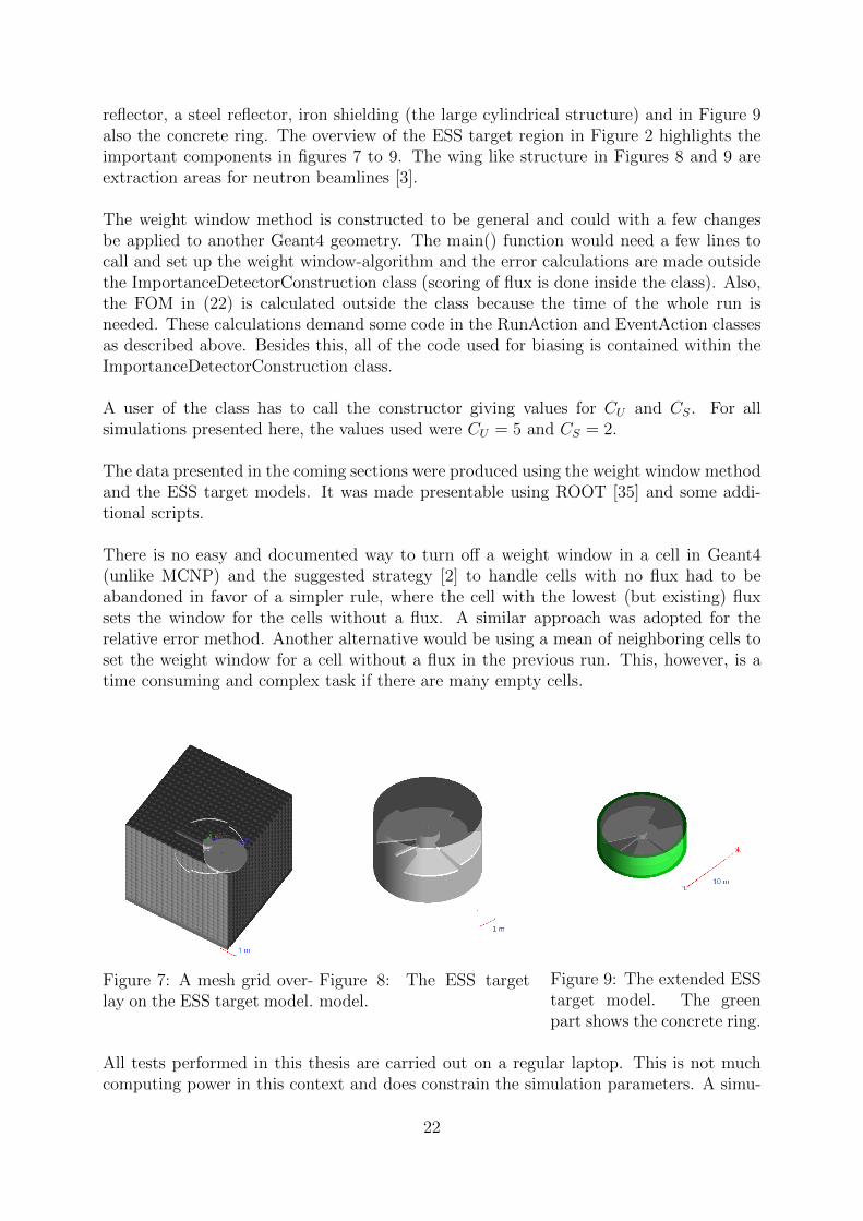
reflector, a steel reflector, iron shielding (the large cylindrical structure) and in Figure 9also the concrete ring. The overview of the ESS target region in Figure 2 highlights theimportant components in figures 7 to 9. The wing like structure in Figures 8 and 9 areextraction areas for neutron beamlines [3].

The weight window method is constructed to be general and could with a few changesbe applied to another Geant4 geometry. The main() function would need a few lines tocall and set up the weight window-algorithm and the error calculations are made outsidethe ImportanceDetectorConstruction class (scoring of flux is done inside the class). Also,the FOM in (22) is calculated outside the class because the time of the whole run isneeded. These calculations demand some code in the RunAction and EventAction classesas described above. Besides this, all of the code used for biasing is contained within theImportanceDetectorConstruction class.

A user of the class has to call the constructor giving values for CU and CS. For allsimulations presented here, the values used were CU = 5 and CS = 2.

The data presented in the coming sections were produced using the weight window methodand the ESS target models. It was made presentable using ROOT [35] and some addi-tional scripts.

There is no easy and documented way to turn off a weight window in a cell in Geant4(unlike MCNP) and the suggested strategy [2] to handle cells with no flux had to beabandoned in favor of a simpler rule, where the cell with the lowest (but existing) fluxsets the window for the cells without a flux. A similar approach was adopted for therelative error method. Another alternative would be using a mean of neighboring cells toset the weight window for a cell without a flux in the previous run. This, however, is atime consuming and complex task if there are many empty cells.

Figure 7: A mesh grid over-lay on the ESS target model.

Figure 8: The ESS targetmodel.

[t][][b]

Figure 9: The extended ESStarget model. The greenpart shows the concrete ring.

All tests performed in this thesis are carried out on a regular laptop. This is not muchcomputing power in this context and does constrain the simulation parameters. A simu-

22

lation like this would benefit from running on a computer cluster, as this would increasethe simulation times and produce results faster. The principle would not change and allresults would carry over to such a simulation..

The setup of the cells and weight windows take about 5 min using this configuration.This number is dependent on the number of cells. The comparatively low number of cellsis chosen with this in regard. This time is excluded from all run times, figures of merit andsuch. This is because this would make it harder to extrapolate results to longer run times.Using relatively short simulations, as many of the cases in this thesis, the additional fiveminutes would be a small fraction of the total time for a longer simulation.

3.2 Results

Figures 10 to 19 show the flux per primary proton and the relative error of the flux for thesimulations. The maps in Figures 10 to 13 are based on data generated from an analogsimulation with run times of 955 s and 47 385 s. These are to be compared with Figures14 to 17 showing the same data but for a simulation using the flux based method. Figures18 and 19 show the relative error results from the relative error based method.

These figures are generated using a 31×31×31 mesh grid. The figures show a plane withdata taken from the middle (cell number 16 in the z direction) cells of the x-y-plane in thetarget model. The axes represent spatial coordinates and the color bars show particle fluxand the calculated error respectively. The figures also show an overlay of a 2D projectionof the geometry of the simulation (compare to Figure 2). N.B. the scales for the figuresshowing flux are shown in logarithmic scale.

The analog method does not populate the whole geometry in the alloted simulation time.Both of the weight window methods manage to do that. The flux based method showsvery little spread of relative errors after the simulation is complete.

The evolution of flux using the flux based method shows that all cells in this plane get aflux after about 7000 s, which is not the case for the analog maps, where there is no fluxin some cells during the whole simulation. A comparison between the flux based methodand the relative error based method shows that the flux based method leads to overallimprovement of the relative error in the cells. In particular, for cells in the outer parts ofthe geometry, there are lower relative errors. One could also note that in the center of thegeometry, the relative error is actually higher than in the analog case. This is a patternalso mentioned in [2].

Figure 20 shows the number of cells without any flux after a given time for the threemethods. The flux based method has no zeros after just two iterations. For a more com-plex model, the shape is more similar to the analog case (see figure 35).

In Figures 22 and 21 the average track weight in a typical outer region cell is shown.For the flux based method, the initial update for the wight window overshoots and thewindow is slightly updated during the whole simulation. One hypothesis would be thatit grows asymptotically to a value where it would be stable. The error based weights are

23

updated more rarely and show a flat pattern between updates.

Figure 10: Flux map of an early analog sim-ulation (955 s).

Figure 11: Relative error map of an earlyanalog simulation (955 s).

Figure 12: Flux map of a late analog simu-lation (47 385 s).

Figure 13: Relative error map of a late ana-log simulation (47 385 s).

Figure 14: Flux map of first weight windowsimulation (896 s).

Figure 15: Relative error map of first weightwindow simulation (896 s).

24

Figure 16: Flux map of the ninth weightwindow simulation (47 394 s).

Figure 17: Relative error map of the ninthweight window simulation (47 394 s).

Figure 18: Relative error map of third rela-tive error based run (17 511 s).

Figure 19: Relative error map of eight rela-tive error based run (46 532 s).

Figure 20: The number of cells that see no flux in the small target model using the twomethods as well as in the analog simulation plotted against the simulation time.

25

In figures 23 and 24, the figures of merit are given for some run times. For the weightwindow methods all measured points are marked. The analog run is shown as a linewithout marks. For the analog run there are 209 points spaced around 300 s apart. Bothmethods show improvements over the analog simulation. FOM1 decreases steadily; withan increasing number of events there is less chance to hit the cells that would give payoffin terms of reduced error. Hence, the more computer time that is diverted to the problem,the less the payoff. The weight window methods show a higher and more stable FOM1.

The second figure of merit is lower for the flux based method and both this and theanalog case show fluctuating figures of merit but without trend. For the relative errorbased method, the trend in the figure of merit is decreasing.

The improvements in the figures of merit are shown in table 3. The figure of merit that hasthe highest time dependence is FOM1 for the analog method. Table 3 show comparisonsof the weight window method with the FOM for the analog case. The difference in theresults in this table are mostly a result of changes in the FOM for the analog case. Thefigure of merit for the flux method is stable while it is steadily decreasing for the analogsimulation (as well as for the relative error based simulation). After the whole simulation,the flux method shows the highest increase in FOM1 relative to the analog simulationwhile the relative error based method decreases FOM2 relative to the analog simulationthe most. FOM1 would be the preferred measure as this takes computing time intoconsideration and is more stable; at least after some time when the shape of the analogFOM1 graph is sufficiently flat. This also shows that the flux based method is better atactually producing lower errors over all.

Table 3: Improvements compared to the analog simulation in FOM1 and FOM2 for thetwo methods for some simulation times.

Flux methodTime FOM1 FOM2

14092 ×(5.62± 0.04) ×(3.15± 0.01)32112 ×(11.50± 0.01) ×(2.54± 0.01)44087 ×(14.60± 0.02) ×(2.64± 0.01)

Relative error methodTime FOM1 FOM2

17510 ×(2.17± 0.01) ×(1.33± 0.01)35763 ×(3.11± 0.01) ×(2.33± 0.01)46532 ×(3.08± 0.01) ×(2.89± 0.01)

Figure 21: The average track weight of atypical cell in the small geometry’s outer re-gions using flux based method.

Figure 22: The average track weight of atypical cell in the small geometry’s outer re-gions using relative error based method.

26

Figure 23: A comparison of the methods ef-ficiency when applied to the small model us-ing FOM1.

Figure 24: A comparison of the methods ef-ficiency when applied to the small model us-ing FOM2.

Figure 25 show the cumulative histogram of the relative errors in the cells. The flat profileof the flux based method is pronounced, most of the cells are in the same error range.The analog simulation has cells that see just a few particles, the steps are longer for thehigh error range. Figure 26 shows the time evolution number of cells with an error ≤ 0.1for the different methods. The number of cells with a reasonable error will increase withrun time. It is clear that the flux based method performs best for runs longer than about40 000 s and improves much faster than its counterpart.

Figure 25: A cumulative histogram of thefraction of cells with a given relative errorwhen applying the two methods, as well asthe analog simulation, on the small mode.

Figure 26: Time evolution of cells with rel-ative error ≤ 0.1, when applying the twomethods on the small model.

As one possible application of the method is to calculate energy spectra, the energy spec-trum produced using the method were compared to the spectrum produced by the analogsimulation. The energy spectrum in Figure 27 is generated from the four detectors shownas bent stripes in Figure 7. The detector is located at a distance of 2 m from the moderator.

The lower section ranging from 10−10 MeV to 10−6 MeV are the moderated spectra. Peaksin this range can be related to the Maxwellian distribution (7). These are neutrons slowed

27

Figure 27: A comparison between the analog and biased spectra in the detectors. Thefigure shows neutron hits in all the detectors with consideration to particle weight. Thespectra are normalized (by setting the maximum peak for the weight window spectrumto to maximum value for the analog spectrum) for easy comparison.

down by the liquid hydrogen and water moderators. The higher peaks come from thetransparency in the steel and iron shielding. Figure 3 shows the cross section of iron andits transparent part can be related to the peaks in Figure 27. The higher energy neutronsin the spectrum come from direct spallation products. These may be in the range up tothe incident proton beam, see section 2.1.2.

The flux of the small model spanned 5 orders of magnitude. The flux in the large modelspans 11 orders of magnitude. The problem remains the same, even if the geometry isslightly changed, but this would be considered a ”hard” problem [28]. It is clear thatthe simulation has to be run longer in this case to produce relevant results, even if usingweight windows.

Figures 28 and 29 show the relative errors of the analog simulation and the flux basedmethod. The flux based method produces a flatter map of relative errors but it is notevident that the errors are generally lower than in the analog case. Close to the center ofthe model the analog case shows lower relative errors. The analog simulation however, hasmany empty cells, which is not the case for the simulation run with the weight windowmethod.

The shape of FOM1 for the flux method now visibly follows the analog shape, as seenin Figure 30. The improvements in the figures of merit are smaller. Table 4 shows theimprovements in the two figures of merit. FOM1 shows a trend to a relatively higherfigure for the weight window method. It is plausible that this trend will go on as in thecase of the smaller model. For FOM2, in Figure 31 it is possible that it follows the same

28

Table 4: Improvements compared to the analog simulation in FOM1 and FOM2 for onemethod for some simulation times.

Flux methodTime FOM1 FOM2

19046 ×(2.10± 0.10) ×(1.58± 0.01)76687 ×(2.43± 0.01) ×(1.58± 0.01)119643 ×(3.98± 0.01) ×(1.79± 0.03)

pattern as in the large model. The trend is downward sloping, but this might change witha longer simulation time.

The qualitative results remain the same and the weights in this model are still updatedafter 150× 103 s (Figure 33). Figures 32 and 33 show the average track weight for sometypical cells in the geometry’s outer regions. The figures show that some cells peak andthen find a low weight window while some others peak and then trend upwards. Thepeak can be explained by the same reasoning as in the small model, the window is settoo high at the first iteration. Some cells will then find an immediate stability while someare still updated when the simulation is finished. These cells are still updated when thesimulation is finished. Both of these cells see no flux in the analog run and gets a weightthat is higher than what would be the result if it had some flux already. This is thencorrected in the following iterations. The cell in Figure 33 is still updated even after thesimulation is finished.

Figure 34 is the cumulative histogram of relative errors for the large model and hasthe same shape as the smaller model (Figure 25) but is shifted to the right. Most cellshave a relative error ≤ 0.4 using the weight window method but very few have an error≤ 0.1. It is clear, however, that the spread in the errors are significantly lowered usingthis method even if the simulation time is short. Figure 35 shows the number of emptycells as a function of time and in this simulation the weight window method needs someiterations to fill all the cells.

Figure 28: Relative error map of the119 927 s long analog run.

Figure 29: Relative error map of the119 643 s long weight window run.

29

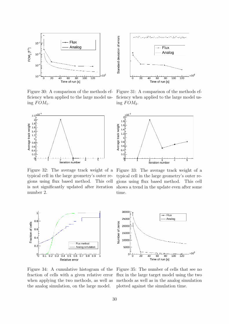
Figure 30: A comparison of the methods ef-ficiency when applied to the large model us-ing FOM1.

Figure 31: A comparison of the methods ef-ficiency when applied to the large model us-ing FOM2.

Figure 32: The average track weight of atypical cell in the large geometry’s outer re-gions using flux based method. This cellis not significantly updated after iterationnumber 2.

Figure 33: The average track weight of atypical cell in the large geometry’s outer re-gions using flux based method. This cellshows a trend in the update even after sometime.

Figure 34: A cumulative histogram of thefraction of cells with a given relative errorwhen applying the two methods, as well asthe analog simulation, on the large model.

Figure 35: The number of cells that see noflux in the large target model using the twomethods as well as in the analog simulationplotted against the simulation time.

30

In practice, a simulation can be run until a sufficient relative error is reached in the leastsampled cell and then invoking a break condition. The update of the weight windows, ifusing the iterative approach, can also be stopped on a condition regarding average trackweight. If this is stable for the whole grid there is no need to update the weight windows.

4 Conclusion

4.1 Conclusion

The methods discussed in this thesis both give an improvement in flux simulations of theESS TDR target region. Less computation time has to be spent to get relevant statistics.For this thesis the simulations have been run for relatively short times on a regular laptop.To get a better simulation results, longer run times or more computer power is needed.

The flux based method dominates the relative error based method with regards to theirrespective figures of merit, hence this is the method primarily suggested for use.

Furthermore, the method is indeed easy to use and implement in principle. There isstill some user judgment needed, but it is possible to implement this as a ’black-box’method taking only the grid and previously generated flux information as input. Theresults presented here are consistent with results presented in [2].

4.2 Outlook and further work

The choice of how to set cells with zero previous flux is based on what was possible withinthe time frame of the thesis work. This could be investigated further as there are someoptions. One considered possibility was to set weight in cells as a mean of neighboringcells. Another option is the one presented by Van Wijk [2]. The best choice for the cellswith no flux is an uninvestigated topic. This is connected to the flux based method asthere is a straightforward way to set the zero flux cells using the relative error method.

There is room for improvement and optimization. For example, the time it takes to setup the mesh grid and give all cells their weights is about 5 min for a 31× 31× 31 on theused computer. This is a property of Geant4 since this time is recorded even when doingno calculations and using the importance sampling algorithm to set all importances to one.

The program was also tested on a multicore computer but does not yet produce properresults. With some corrections it could work in such an environment. Furthermore themethod does not perform any energy dependent weighting. This would be a good additionto the procedure.

The method shows good improvement of flux calculations on the ESS target model. Itproduces correct spectra for neutron energies and is indeed easy to use and implementwithout much further consideration on any geometry. These methods should be able tofind use in practical neutron flux simulations. With some further work this method orsomething like it could be included in the Geant4 framework.

31

References

[1] Geant4 Collaboration. Geant4 User’s Guide for Application Developers Version:10.1. Geant4 Collaboration, 2014.

[2] AJ Van Wijk, Gert Van den Eynde, and JE Hoogenboom. An easy to imple-ment global variance reduction procedure for MCNP. Annals of Nuclear Energy,38(11):2496–2503, 2011.

[3] Steve Peggs, R Kreier, C Carlile, R Miyamoto, A Pahlsson, M Trojer, andJG Weisend II. ESS technical design report. European Spallation Source ESS AB,2013.

[4] Konstantin Batkov, Alan Takibayev, Luca Zanini, and Ferenc Mezei. Unperturbedmoderator brightness in pulsed neutron sources. Nuclear Instruments and Methods inPhysics Research Section A: Accelerators, Spectrometers, Detectors and AssociatedEquipment, 729:500–505, 2013.

[5] Gunter Siegfried Bauer. Physics and technology of spallation neutron sources. Nu-clear Instruments and Methods in Physics Research Section A: Accelerators, Spec-trometers, Detectors and Associated Equipment, 463(3):505–543, 2001.

[6] R Arthur Forster, Lawrence J Cox, Richard F Barrett, Thomas E Booth, Judith FBriesmeister, Forrest B Brown, Jeffrey S Bull, Gregg C Geisler, John T Goorley,Russell D Mosteller, et al. MCNP� version 5. Nuclear Instruments and Methods inPhysics Research Section B: Beam Interactions with Materials and Atoms, 213:82–86,2004.

[7] FLUKA Collaboration et al. FLUKA manual. ASCII or. pdf file available fromFLUKA website and contained in FLUKA package, 2011.

[8] Tatsuhiko Sato, Koji Niita, Norihiro Matsuda, Shintaro Hashimoto, Yosuke Iwamoto,Shusaku Noda, Tatsuhiko Ogawa, Hiroshi Iwase, Hiroshi Nakashima, Tokio Fukahori,et al. Particle and heavy ion transport code system, PHITS, version 2.52. Journalof Nuclear Science and Technology, 50(9):913–923, 2013.

[9] Nataliia Cherkashyna, Richard J Hall-Wilton, Douglas D DiJulio, Anton Khaplanov,Dorothea Pfeiffer, Julius Scherzinger, Carsten P Cooper-Jensen, Kevin G Fissum,Stuart Ansell, Erik B Iverson, et al. Overcoming high energy backgrounds at pulsedspallation sources. arXiv preprint arXiv:1501.02364, 2015.

[10] JE Beaver and HB Hupf. Production of 99mtc on a medical cyclotron: a feasibilitystudy. Journal of Nuclear Medicine, 12(11):739–741, 1971.

[11] Richard Van Noorden. The medical testing crisis. Nature, 504(7479):202–204, 2013.

[12] Neal Jay Carron. An introduction to the passage of energetic particles through matter.CRC Press, Boca Raton, first edition, 2006.

[13] Alvin M Weinberg and Eugene Paul Wigner. The physical theory of neutron chainreactors. Chicago Univ. Press, Chicago, first edition, 1958.

32

[14] John R Lamarsh and Anthony John Baratta. Introduction to nuclear engineering.Prentice Hall, Upper Saddle River, third edition, 2001.

[15] JM Carpenter. Neutron production, moderation, and characterization of sources.Argonne National Laboratory, 2004.

[16] Kenneth S Krane. Introductory nuclear physics. John Wiley and Sons Inc., NewYork, second edition, 1987.

[17] Aatos Heikkinen, Nikita Stepanov, and Johannes Peter Wellisch. Bertini intra-nuclearcascade implementation in geant4. arXiv preprint nucl-th/0306008, 2003.

[18] Gunter Siegfried Bauer. Neutron sources. INIS collection, 30(47), 1999.

[19] Norbert Ensslin. The origin of neutron radiation, chapter 11, passive nondestructiveassay nuclear materials. Technical report, NUREG/CR-5550, 1991.

[20] JW Boldeman. Accelerator driven nuclear energy systems. Energy For Ever: Techno-logical Challenges of Sustainable Growth, Australian Academy of Technological Sci-ences and Engineering, Academy Symposium, 1998.

[21] Bertram Terence Martin Willis and Colin J Carlile. Experimental neutron scattering.Oxford Univ. Press, Oxford, first edition, 2009.

[22] James J Duderstadt and Louis J Hamilton. Nuclear reactor analysis. John Wileyand Sons, Inc., New York, first edition, 1976.

[23] KH Beckurts and K Wirtz. Production and nuclear interaction of neutrons. InNeutron Physics, pages 1–21. Springer, 1964.

[24] Igor Koprivnikar and E Schachinger. The biological shield of a high-intensity spal-lation source: a monte carlo design study. Nuclear Instruments and Methods inPhysics Research Section A: Accelerators, Spectrometers, Detectors and AssociatedEquipment, 487(3):571–584, 2002.

[25] National nuclear data center. http://www.nndc.bnl.gov/sigma/. Accessed: 2015-05-21.

[26] Roger Eckhardt. Stan Ulam, John von Neumann, and the monte carlo method. LosAlamos Science, 15:131–136, 1987.

[27] Ivan Lux and Laszlo Koblinger. Monte Carlo particle transport methods: neutronand photon calculations, volume 102. CRC press, Boca Ration, first edition, 1991.

[28] Douglas E Peplow. Comparison of hybrid methods for global variance reduction inshielding calculations. Transactions of the American Nuclear Society, 107:512, 2012.

[29] Monte Carlo Team. MCNP–a general Monte Carlo N-particle transport code, version5. Book MCNP-A General Monte Carlo N-Particle Transport Code Version, 5, 2003.

[30] Andrew Davis and Andrew Turner. Comparison of global variance reduction tech-niques for Monte Carlo radiation transport simulations of ITER. Fusion Engineeringand Design, 86(9):2698–2700, 2011.

33

[31] James Bucklew. Introduction to rare event simulation. Springer Science & BusinessMedia, New York, first edition, 2004.

[32] Pierre L’Ecuyer and Bruno Tuffin. Splitting with weight windows to control the likeli-hood ratio in importance sampling. In Proceedings of the 1st international conferenceon Performance evaluation methodolgies and tools, page 21. ACM, 2006.

[33] Marc A Cooper and Edward W Larsen. Automated weight windows for global montecarlo particle transport calculations. Nuclear science and engineering, 137(1):1–13,2001.

[34] TL Becker and EW Larsen. The application of weight windows to “global” montecarlo problems. In Proc. Conf. Advances in Mathematics, Computational Methods,and Reactor Physics. American Nuclear Society Saratoga Springs, New York, 2009.

[35] Rene Brun and Fons Rademakers. ROOT—an object oriented data analysis frame-work. Nuclear Instruments and Methods in Physics Research Section A: Accelerators,Spectrometers, Detectors and Associated Equipment, 389(1):81–86, 1997.

34