Forschungsinstitut zur Zukunft der ArbeitInstitute for the Study of Labor

DI

SC

US

SI

ON

P

AP

ER

S

ER

IE

S

Gender Gaps in the Effects of Childhood Family Environment: Do They Persist into Adulthood?

IZA DP No. 10313

October 2016

Anne Ardila BrenøeShelly Lundberg

Gender Gaps in the Effects of

Childhood Family Environment: Do They Persist into Adulthood?

Anne Ardila Brenøe University of Copenhagen

Shelly Lundberg

University of California, Santa Barbara and IZA

Discussion Paper No. 10313 October 2016

IZA

P.O. Box 7240 53072 Bonn

Germany

Phone: +49-228-3894-0 Fax: +49-228-3894-180

E-mail: iza@iza.org

Any opinions expressed here are those of the author(s) and not those of IZA. Research published in this series may include views on policy, but the institute itself takes no institutional policy positions. The IZA research network is committed to the IZA Guiding Principles of Research Integrity. The Institute for the Study of Labor (IZA) in Bonn is a local and virtual international research center and a place of communication between science, politics and business. IZA is an independent nonprofit organization supported by Deutsche Post Foundation. The center is associated with the University of Bonn and offers a stimulating research environment through its international network, workshops and conferences, data service, project support, research visits and doctoral program. IZA engages in (i) original and internationally competitive research in all fields of labor economics, (ii) development of policy concepts, and (iii) dissemination of research results and concepts to the interested public. IZA Discussion Papers often represent preliminary work and are circulated to encourage discussion. Citation of such a paper should account for its provisional character. A revised version may be available directly from the author.

IZA Discussion Paper No. 10313 October 2016

ABSTRACT

Gender Gaps in the Effects of Childhood Family Environment: Do They Persist into Adulthood?

We examine the differential effects of family disadvantage on the education and adult labor market outcomes of men and women using high-quality administrative data on the entire population of Denmark born between 1966 and 1995. We link parental education and family structure during childhood to male-female and brother-sister differences in teenage outcomes, educational attainment, and adult earnings and employment. Our results are consistent with U.S. findings that boys benefit more from an advantageous family environment than do girls in terms of the behavior and grade-school outcomes. Father’s education, which has not been examined in previous studies, is particularly important for sons. However, we find a very different pattern of parental influence on adult outcomes. The gender gaps in educational attainment, employment, and earnings are increasing in maternal education, benefiting daughters. Paternal education decreases the gender gaps in educational attainment (favoring sons) and labor market outcomes (favoring daughters). We conclude that differences in the behavior of school-aged boys and girls are a poor proxy for differences in skills that drive longer-term outcomes. JEL Classification: I20, J1, J2, J3 Keywords: gender gap, parental education, family structure, education,

labor market outcomes Corresponding author: Anne Ardila Brenøe Department of Economics University of Copenhagen Øster Farimagsgade 5, Building 26 1353 Copenhagen K Denmark E-mail: aab@econ.ku.dk

1 Introduction

Over the past century, the barriers to women’s educational and employment opportu-

nities have been dramatically lowered in most of the developed world. Women continue

to have lower rates of labor force participation and earn lower pay than men, but new

gender gaps that favor women have opened up in education. Young men lag behind

young women in academic achievement, and contributing factors include less engage-

ment in school, a gap in homework hours and the substitution of time spent playing

video games for time spent reading (OECD, 2015). Women are now more likely than

men to complete secondary education and to graduate from college in almost all OECD

countries. In the United States, 39 percent of women aged 25 to 29 have a Bachelor’s

degree or more, compared to 32 percent of men (U.S. Census Bureau, 2015).

Recent studies have focused on the behavioral differences between school-aged boys

and girls, arguing that a gender gap in “non-cognitive skills” contributes to the scholas-

tic underperformance of boys by increasing the costs of school persistence and perfor-

mance (Goldin et al., 2006; Becker et al., 2010). Family disadvantage is strongly neg-

atively associated with early social and behavioral skills for both boys and girls, and

it has been suggested that trends in family structure, and in particular the increasing

prevalence of single parent families, may have a particularly deleterious effect on the

skill development of boys (Bertrand and Pan, 2013; Autor and Wasserman, 2013). If

exposure to father absence, povery, or poor neighborhoods harm boys more than girls,

then changes in the living arrangements of children over time may explain part of the

growing gender gap in educational attainment. Put differently, these recent studies ad-

vance the hypothesis that boys benefit more from an advantageous family environment

than do girls.

Autor et al. (2016) examine this hypothesis using sibling fixed-effects models and

a sample of students in Florida, and find that early family structure and mother’s

education do have significantly larger effects on a variety of school outcomes for boys

than for their sisters. However, there is also evidence that the greater impact of family

1

background on boys is most relevant for school-age behavior in the United States, and

does not extend to longer-term outcomes such as educational attainment (Lundberg,

2016). With our analysis, we contribute to this literature in three important ways.

First, we re-examine and confirm gender differences in the impacts of family envi-

ronment on school-age outcomes for Denmark, another OECD country with different

social institutions and lower poverty prevalence, especially among single-parent fami-

lies.1 Second, our main contribution is to examine a broad range of adult outcomes for

the total population as well as for large samples of full siblings. Third, the richness of

the data makes it possible to study potential differences in family environment effects

across cohorts. Administrative data on the entire population of Denmark from 1980

to 2011 with cohorts born from 1966 to 1995 enables us to link parental education and

family structure during childhood to male-female differences in adolescent outcomes,

educational attainment, and adult earnings and employment. A significant advantage

of the Danish administrative data is that we are able to add paternal education, which

is not available for large subsets of the American samples, to our indicators of family

background.

Denmark has experienced trends in relative male and female educational attain-

ment and single-parent households that are similar to those in the U.S., though the

educational and labor market environments are distinct.2 The more comprehensive

social safety net may moderate the impacts of family disadvantage on child outcomes.

Though female labor force participation rates in Denmark are high, women are more

likely to work part-time than in the U.S. and also more likely to work in the public

sector. On the other hand, we expect that any developmental process that renders

boys more vulnerable to adverse family environments should be a very general one

that is manifest in diverse institutional environments. For instance, Landersø and

Heckman (2016) find that despite great social policy differences, the influence of family

background on educational attainment is similar in Denmark and the U.S.

1See e.g. Rossin-Slater and Wust (2014) on child support obligations in Denmark.2Appendix Figure A1 illustrates the reversal in the gender gap in highest completed education by age 29

for Denmark.

2

We find, as do Autor et al. (2016) and Lundberg (2016), that adolescent boys

appear to be more sensitive than girls to family environment. However, we find a

very different pattern of parental influence on adult outcomes such as educational

attainment, college graduation, employment, and earnings. Gender differences in the

effects of family structure are weak and when we do find significant differential effects

they show greater responsiveness for women. Maternal education consistently has a

greater impact on the education and employment of daughters relative to sons and

this effect is stable across cohorts. Paternal education has some significant, though

smaller, effects on the gender education gap that favor sons (and that decline over

time), but has larger positive effects on the employment and earnings of daughters.

Estimates based on the total population are similar to those obtained from a sample

of full siblings controlling for family fixed effects. This suggests that the selection of

boys and girls across different family types is not biasing our estimates of the gender

gap in the effects of family environment in the full sample.

We conclude that, although there are gender differences in responses to parental

resources and family structure, they do not conform to the simple story that the skill

development of boys is particularly vulnerable to family disadvantage. Nor is there

any evidence, in the Danish context, that changes in family structure have played any

role in the growing education gap in favor of girls. Our results are consistent with an

alternative hypothesis in which maternal education and other family resources have a

strong moderating effect on behavioral problems in school that are much more typical

of boys than girls. These parental influences become less important as the children

become adults, and there is no indication that these early behavior gaps imply less long-

term skill acquisition by boys, relative to girls. Instead, the determinants of educational

attainment include positive effects of same-sex parental education that may reflect role-

modelling. The greater responsiveness, in turn, of women’s employment and earnings

to parental education than the labor market outcomes of adult men, indicates that

female labor market behavior in Denmark is more elastic than men’s with respect to

early influences.

3

2 Family Background and Child Outcomes: Is

There a Gender Dimension?

Boys begin school with less-developed social and behavioral skills than girls, and these

gaps persist through elementary school and explain much of the gender differential

in early academic outcomes (DiPrete and Jennings, 2012). Girls consistently receive

higher grades, are less likely to repeat grades or to be placed in special education

classes, and are less likely to get in trouble at school. There are clear behavioral

patterns underlying these disparate outcomes—girls spend more time on homework,

are more likely to read for pleasure, and exhibit a greater degree of self-discipline in

school.3 Attempts to explain the emergence of a gender gap favoring women in col-

lege attendance and completion have appealed to these gender differences in academic

achievement and school discipline as evidence of a “non-cognitive skill” deficit that in-

creases the effective costs of attending and succeeding in school for boys (Goldin et al.,

2006; Becker et al., 2010).

In addition to this gender skill gap, there are also strong socioeconomic gradients in

early social skills, attention, and school engagement. These skill differences can explain

a portion of the socioeconomic differences in young adult outcomes such as arrests and

high school completion (Duncan and Magnuson, 2011). Autor and Wasserman (2013)

suggest a new explanation for the trend in the relative educational attainment of men

and women based on these socioeconomic skill differentials and trends in family struc-

ture. They hypothesize that, as the prevalence of single parent families has increased in

the U.S. (and elsewhere), economic stresses have increased for children in lower income

households and their access to paternal time and attention has decreased. If the skill

development of boys is affected more by father absence or family disadvantage than

the skill development of girls, then changes in the living arrangements of children over

time may play a role in the growing education gender gap. Bertrand and Pan (2013)

3Duckworth and Seligman (2006) use several measures of self-discipline to document this gender difference,including self-reports, teacher and parent reports, and a delay of gratification test.

4

provide supportive empirical evidence, showing that living with a single mother or a

young mother has a much larger effect on externalizing behavior and school suspen-

sions for boys than for girls. They interpret the negative behavioral impact of father

absence and young mothers as evidence that the non-cognitive skills development of

boys is particularly sensitive to family disadvantage.

It is not clear what the mechanisms might be that make boys more vulnerable to

adverse environments in childhood. One possibility is that gender differences in de-

velopmental trajectories may make girls, who enter school more mature in language

skills and emotional regulation, inherently more resilient to disadvantage. Alterna-

tively, there may be socioeconomic differences in the way that parents invest in young

boys and girls. Baker and Milligan (2013) find that parents in three countries, includ-

ing the U.S., spend more time in teaching activities with girls than with boys at very

young ages. Bertrand and Pan (2013) find that single mothers spend more time with

daughters than with sons and report less emotional closeness with sons. Finally, there

may be cultural factors that lead boys, in particular, to develop negative attitudes to

school in low income or single parent families or that inhibit the educational aspirations

of boys relative to girls (DiPrete and Buchmann, 2013). Fortin et al. (2015) find that

much of the gender divergence in high school GPA distributions can be attributed to

the increasingly ambitious post-school plans of girls relative to boys.

Autor et al. (2016) re-examine this “vulnerable boys” hypothesis using data for

a large sample of children in Florida that links birth certificates with academic and

health records. Using a variety of measures of family environment (including mother’s

education, marital status at birth, father presence, and an SES index), neighborhood

income and school quality, they find that early family structure and mother’s education

do have significantly larger effects on a variety of school outcomes for boys than for their

sisters, including school suspensions and absences, in both OLS and family fixed effects.

There is a larger payoff for boys to having a college graduate mother for a broad set

of academic outcomes, including kindergarten readiness and grades. They find similar

patterns of differential gender impacts of low-income neighborhoods and poor-quality

5

schools, and conclude that family disadvantage has larger impacts on the outcomes

of boys relative to girls throughout school. Though they are unable to examine later

outcomes, including college attainment, earnings, and labor force participation, Autor

et al. (2016) suggest that early gender differences in behavioral and school outcomes

are likely to have implications for adult outcomes.

Other studies cast some doubt on this final speculation, however. Riphahn and

Schwientek (2015) examine the growth of the gender education gap in Germany, and

find that the reversal of this gap has been most pronounced in disadvantaged groups.

However, they find no link between family background and gender differences in edu-

cational attainment in the individual data. Lundberg (2016), using the National Lon-

gitudinal Study of Adolescent to Adult Health (Add Health), finds that father absence

is associated with more negative outcomes for school-age boys when the measures are

similar to those used in previous studies—problems in school and school suspensions.

Girls, on the other hand, are more likely to score higher on indicators of depression

when their father is absent, and particularly when they are in a stepfather household.

Differential vulnerability to father absence appears to depend on whether the outcomes

are related to externalizing behavior, which is more typical for boys, or internalizing

behavior, which is a more common response to stress for girls. Lundberg (2016) finds

that neither of these patterns of adolescent response have any significant implications

for educational outcomes, however: father absence has no differential impact on college

graduation in cross-sectional or sibling fixed-effects models. The effects of school qual-

ity follow a similar pattern: the gender gap in suspensions and educational aspirations

is higher in low quality schools than in high quality schools, but there is no differential

gender impact of school quality on educational attainment.4

Consequently, it is not clear whether gender differences in the effects of childhood

environment persist into adulthood. Using Danish administrative data, we will test

4Fan et al. (2015) take a different approach to the emerging gender gap, postulating that boys maybe more adversely affected by mother’s employment in childhood. They find evidence for a more positiveassociation between mother’s work and girl’s education in Norwegian administrative data using family fixed-effect models. They do not, however, control for mother’s education, which we find is a stronger predictorof daughters’ outcomes than of sons’.

6

the hypothesis that males benefit more from mother’s and father’s education and from

having married parents at birth than do females in terms of adult outcomes. For

outcomes with a gender gap favoring women, the relevant hypothesis is that the gender

gap is smaller for individuals from advantageous family backgrounds. We also test

whether any differential effects of family disadvantage by gender have varied across

cohorts in ways that could explain trends in the gender gap in education.

3 Data

We use Danish administrative data covering the entire population born in Denmark be-

tween 1966 and 1995 to examine both outcomes during adolescence and the longer-term

consequences of parental resources and family structure in early life. One important

feature of this dataset is that we are able to link each child to his or her biological

parents (both mother and father) and siblings. Moreover, we observe educational and

labor market outcomes for each year, and can track with whom each individual lives.

3.1 Family Childhood Environment

We measure three dimensions of childhood family environment: parental education,

marital status at birth, and immigrant status. In the administrative data, we observe

the father’s as well as the mother’s education for almost all children, and are able to

track family structure from birth through childhood.

We group each parent’s education into three categories: less than 12 years of edu-

cation (<HS ) corresponding to high school dropouts in the U.S.; high school graduate

(HS ) which may include some vocational training or 2 year college; and bachelor’s

degree graduate or more (BA) corresponding to a degree from a four year college in

the U.S. The latter category covers professional bachelor degrees (e.g. school teacher,

nursing, physiotherapist, social worker) as well as university and business school de-

grees.

Our primary measure of family structure is parental marital status at birth. For

7

models using our sample of full siblings, we use parents’ marital status at the birth of

the youngest of their joint children. We choose this alternative definition of marital

status because it is very common in Denmark to marry after the birth of the first

child and eventual marital status seems to provide a better indicator of the parental

relationship as shared by siblings. As almost all parents with more than one child are

either married or cohabiting at the time of the youngest of their joint children, we only

distinguish between having married and non-married parents.5.

For the models of adult outcomes we consider family structure measured at age

12 as well as parental marital status at birth.6 For childhood family structure, we

distinguish between three types: traditional families where children live with both

biological parents (Trad), with no distinction between married and cohabiting parents;

step-families in which children live with one biological parent and a step-parent (Step);

and single parent families (Single). Using childhood family structure, though it may

be endogenous with respect to child outcomes, allows us to include birth cohorts going

back to 1966, while marital status at birth is observed only in the medical birth registry

which begins in 1973. Family structure at birth and at age 12 are strongly correlated,7

and results using both measures are quantitatively similar.

Finally, we consider the immigrant background of both parents separately. The

composition of immigrants to Denmark has changed considerably over time. For our

earliest cohorts, immigration flows are small and mainly from Western countries (pre-

dominantly other Scandinavian countries, Germany, Great Britain, and the U.S.).8

Later, immigration expanded to include guest workers and refugees from non-Western

countries (with the majority from Turkey, Pakistan, Lebanon, Iraq, and former Yu-

5Less than two percent of the sibling sample have parents who never cohabit and who are never marriedat any of the childbirths

6More precisely, family structure at age 12 is measured on January 1st of the year the child turns 13. Wealso considered family structure at age 16 with very similar results.

7Of those last born children who were born to married (non-married) parents, 80.88 (60.69) percent livein a traditional family at age 12, while 7.48 (14.46) percent live in a step family and 11.64 (24.85) percentlive with a single parent.

8Statistics Denmark defines “Western” countries as European Union countries by 1995, Andorra, Aus-tralia, Canada, Iceland, Liechtenstein, Monaco, New Zealand, Norway, San Marino, Switzerland, USA, andVatican City.

8

goslavia). Of the cohort born in 1966, 3.2 (2.6) percent have an immigrant mother

(father) of whom 64.4 (54.4) percent originate from a Western country. For the last

birth cohort in our sample (born in 1995), 13.8 (13.6) percent have an immigrant

mother (father) of whom only 20.1 (22.8) percent come from a Western country.

3.2 Outcome Variables: From Adolescence through Adult-

hood

The outcomes of interest fall into two groups: 1) School and behavioral outcomes

measured in adolescence and 2) Educational attainment and labor market outcomes,

primarily measured at age 27. Since these outcomes span from age 16 through age

27 (and in some specifications through age 40) and come from several administrative

registers, different birth cohorts will be used in analyses of outcomes in adolescence

and adulthood; Appendix Table A1 summarizes the cohorts used for each part of the

analysis.9 We have one outcome that is available for all cohorts, completion of grade

9 on time, and we use this outcome to examine whether the gender gap in the effects

of family environment has changed over time.

In Denmark, the first nine years of schooling constitute primary school and are

mandatory. Children are required to start first grade the year they turn 7, though

parents are able to apply for an exemption such that their child starts school a year

earlier or later. Boys are about twice as likely to delay school start compared to girls

(Dee and Sievertsen, 2015). Grade repetition is very rare; Simonsen et al. (2015) show

that on average less than 0.5 percent are retained or delayed for each grade level from

grade 1 to 9. Whether the child completes grade 9 on time is a marker of academic

achievement that reflects a combination of early school readiness and success in school

progression, and is strongly correlated with final educational attainment.

At the end of primary school, students take the final grade 9 exam, which is the

9When we refer to outcomes at a certain age, we always refer to the age the individual turns during theparticular year. Thus, grade 9 outcomes are measured at age 15 for about half of the sample, since the schoolyear ends in June.

9

same across the country and is required for all students who continue to academic

high school.10 Our second school outcome is the overall GPA obtained at the end of

grade 9 (based on all grades received both from teacher assessment and final exams).11

Other early outcomes include indicators of having received a diagnosis for behavioral

and emotional disorders at a hospital12 and attending special education during grade

9.13 Since the administrative data on grade 9 GPA begins in 2002, we consider birth

cohorts born from 1986 to 1995 for this part of the analysis.

After primary school, students can choose to continue to academic high school,

which takes three years, or vocational training programs of differing lengths (predom-

inantly 13 or 13.5 years). A diploma from the academic high school is necessary to

apply for university. A bachelor’s degree from university takes three years (i.e. 15 years

of completed education) and a master’s degree takes two additional years. Instead of

university, it is possible for academic high school graduates to take a two year college

degree or to enter vocational training.

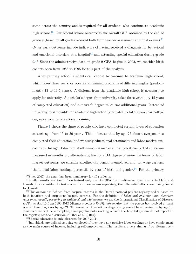
Figure 1 shows the share of people who have completed certain levels of education

at each age from 15 to 30 years. This indicates that by age 27 almost everyone has

completed their education, and we study educational attainment and labor market out-

comes at this age. Educational attainment is measured as highest completed education

measured in months or, alternatively, having a BA degree or more. In terms of labor

market outcomes, we consider whether the person is employed and, for wage earners,

the annual labor earnings percentile by year of birth and gender.14 For the primary

10Since 2007, the exam has been mandatory for all students.11Similar results are found if we instead only use the GPA from written national exams in Math and

Danish. If we consider the test scores from these exams separately, the differential effects are mainly foundfor Danish.

12This outcome is defined from hospital records in the Danish national patient registry and is based onboth inpatient and outpatient hospital records. For the definition of behavioral and emotional disorderswith onset usually occurring in childhood and adolescence, we use the International Classification of Diseases(ICD) version 10 from 1994-2012 (diagnosis codes F90-98). We require that the person has received at leastone of these diagnoses by age 21; 92 percent of those with a diagnosis by age 21 have received it by age 16.This measure will be incomplete, since psychiatrists working outside the hospital system do not report tothe registry; see the discussion in Obel et al. (2015).

13Special education is only observed for 2007-2011.14Individuals are defined as being employed if they have any positive labor earnings or have employment

as the main source of income, including self-employment. The results are very similar if we alternatively

10

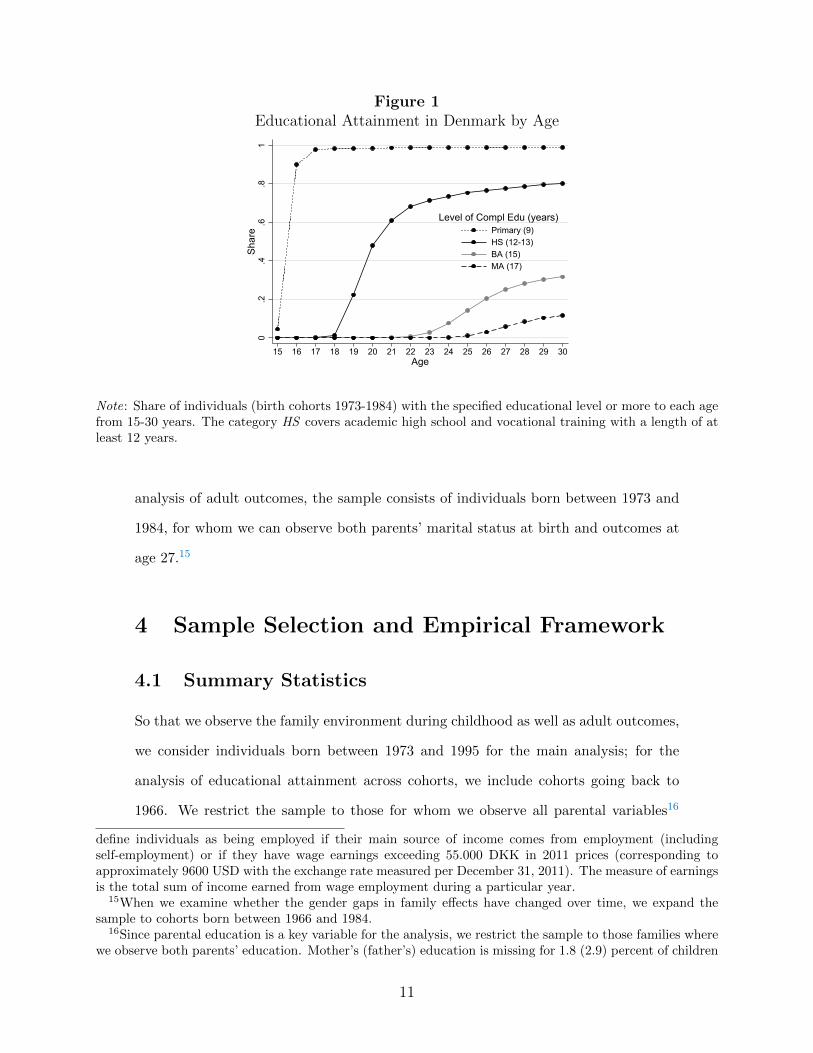
Figure 1Educational Attainment in Denmark by Age

0.2

.4.6

.81

Shar

e

15 16 17 18 19 20 21 22 23 24 25 26 27 28 29 30Age

Primary (9)HS (12-13)BA (15)MA (17)

Level of Compl Edu (years)

Note: Share of individuals (birth cohorts 1973-1984) with the specified educational level or more to each agefrom 15-30 years. The category HS covers academic high school and vocational training with a length of atleast 12 years.

analysis of adult outcomes, the sample consists of individuals born between 1973 and

1984, for whom we can observe both parents’ marital status at birth and outcomes at

age 27.15

4 Sample Selection and Empirical Framework

4.1 Summary Statistics

So that we observe the family environment during childhood as well as adult outcomes,

we consider individuals born between 1973 and 1995 for the main analysis; for the

analysis of educational attainment across cohorts, we include cohorts going back to

1966. We restrict the sample to those for whom we observe all parental variables16

define individuals as being employed if their main source of income comes from employment (includingself-employment) or if they have wage earnings exceeding 55.000 DKK in 2011 prices (corresponding toapproximately 9600 USD with the exchange rate measured per December 31, 2011). The measure of earningsis the total sum of income earned from wage employment during a particular year.

15When we examine whether the gender gaps in family effects have changed over time, we expand thesample to cohorts born between 1966 and 1984.

16Since parental education is a key variable for the analysis, we restrict the sample to those families wherewe observe both parents’ education. Mother’s (father’s) education is missing for 1.8 (2.9) percent of children

11

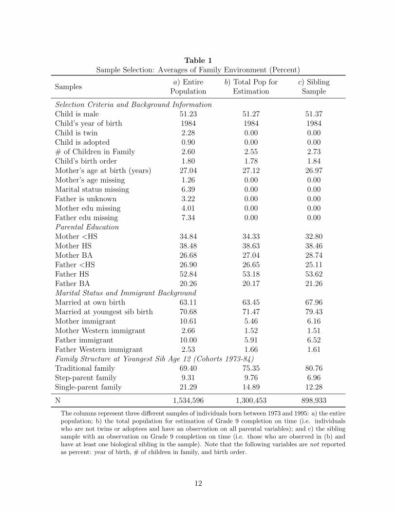
Table 1Sample Selection: Averages of Family Environment (Percent)

Samplesa) Entire

Populationb) Total Pop for

Estimationc) SiblingSample

Selection Criteria and Background InformationChild is male 51.23 51.27 51.37Child’s year of birth 1984 1984 1984Child is twin 2.28 0.00 0.00Child is adopted 0.90 0.00 0.00# of Children in Family 2.60 2.55 2.73Child’s birth order 1.80 1.78 1.84Mother’s age at birth (years) 27.04 27.12 26.97Mother’s age missing 1.26 0.00 0.00Marital status missing 6.39 0.00 0.00Father is unknown 3.22 0.00 0.00Mother edu missing 4.01 0.00 0.00Father edu missing 7.34 0.00 0.00Parental EducationMother <HS 34.84 34.33 32.80Mother HS 38.48 38.63 38.46Mother BA 26.68 27.04 28.74Father <HS 26.90 26.65 25.11Father HS 52.84 53.18 53.62Father BA 20.26 20.17 21.26Marital Status and Immigrant BackgroundMarried at own birth 63.11 63.45 67.96Married at youngest sib birth 70.68 71.47 79.43Mother immigrant 10.61 5.46 6.16Mother Western immigrant 2.66 1.52 1.51Father immigrant 10.00 5.91 6.52Father Western immigrant 2.53 1.66 1.61Family Structure at Youngest Sib Age 12 (Cohorts 1973-84)Traditional family 69.40 75.35 80.76Step-parent family 9.31 9.76 6.96Single-parent family 21.29 14.89 12.28

N 1,534,596 1,300,453 898,933

The columns represent three different samples of individuals born between 1973 and 1995: a) the entirepopulation; b) the total population for estimation of Grade 9 completion on time (i.e. individualswho are not twins or adoptees and have an observation on all parental variables); and c) the siblingsample with an observation on Grade 9 completion on time (i.e. those who are observed in (b) andhave at least one biological sibling in the sample). Note that the following variables are not reportedas percent: year of birth, # of children in family, and birth order.

12

and include only families without adopted children and only singleton births.17 For

the main analysis, we consider this sample (referred to as the total population) as well

as the subsample of families with at least two full siblings (i.e. children with the same

mother and same father; referred to as the sibling sample).

Figure 2Gender Gap in Highest Completed Education (in Months) at 27

-6-4

-20

Boy-

Girl

Gap

in C

ompl

Edu

by

27 (M

onth

s)

1966-70 71-74 75-78 79-84Birth Cohort

Mom <HS Mom HS Mom BAMean by

(a) By Maternal Education

-6-4

-20

Boy-

Girl

Gap

in C

ompl

Edu

by

27 (M

onth

s)

1966-70 71-74 75-78 79-84Birth Cohort

Single 12 Step 12 Trad 12Mean by

(b) By Family Structure

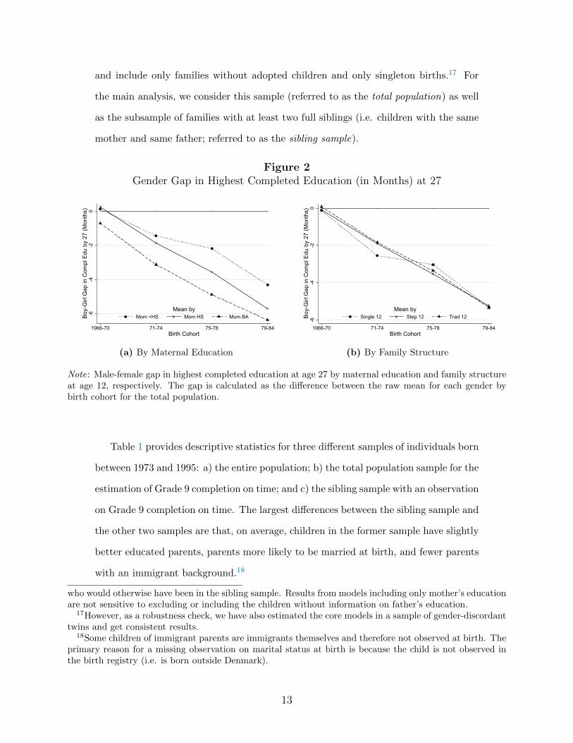
Note: Male-female gap in highest completed education at age 27 by maternal education and family structureat age 12, respectively. The gap is calculated as the difference between the raw mean for each gender bybirth cohort for the total population.

Table 1 provides descriptive statistics for three different samples of individuals born

between 1973 and 1995: a) the entire population; b) the total population sample for the

estimation of Grade 9 completion on time; and c) the sibling sample with an observation

on Grade 9 completion on time. The largest differences between the sibling sample and

the other two samples are that, on average, children in the former sample have slightly

better educated parents, parents more likely to be married at birth, and fewer parents

with an immigrant background.18

who would otherwise have been in the sibling sample. Results from models including only mother’s educationare not sensitive to excluding or including the children without information on father’s education.

17However, as a robustness check, we have also estimated the core models in a sample of gender-discordanttwins and get consistent results.

18Some children of immigrant parents are immigrants themselves and therefore not observed at birth. Theprimary reason for a missing observation on marital status at birth is because the child is not observed inthe birth registry (i.e. is born outside Denmark).

13

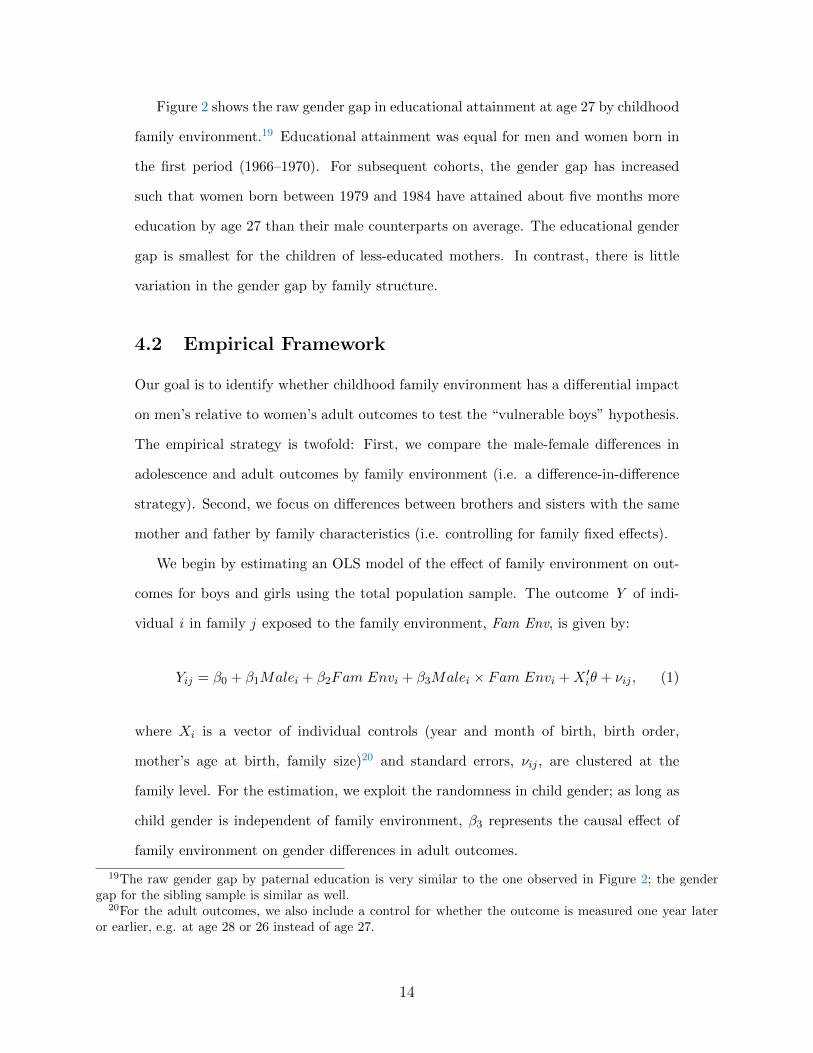
Figure 2 shows the raw gender gap in educational attainment at age 27 by childhood

family environment.19 Educational attainment was equal for men and women born in

the first period (1966–1970). For subsequent cohorts, the gender gap has increased

such that women born between 1979 and 1984 have attained about five months more

education by age 27 than their male counterparts on average. The educational gender

gap is smallest for the children of less-educated mothers. In contrast, there is little

variation in the gender gap by family structure.

4.2 Empirical Framework

Our goal is to identify whether childhood family environment has a differential impact

on men’s relative to women’s adult outcomes to test the “vulnerable boys” hypothesis.

The empirical strategy is twofold: First, we compare the male-female differences in

adolescence and adult outcomes by family environment (i.e. a difference-in-difference

strategy). Second, we focus on differences between brothers and sisters with the same

mother and father by family characteristics (i.e. controlling for family fixed effects).

We begin by estimating an OLS model of the effect of family environment on out-

comes for boys and girls using the total population sample. The outcome Y of indi-

vidual i in family j exposed to the family environment, Fam Env, is given by:

Yij = β0 + β1Malei + β2Fam Envi + β3Malei × Fam Envi +X ′iθ + νij , (1)

where Xi is a vector of individual controls (year and month of birth, birth order,

mother’s age at birth, family size)20 and standard errors, νij , are clustered at the

family level. For the estimation, we exploit the randomness in child gender; as long as

child gender is independent of family environment, β3 represents the causal effect of

family environment on gender differences in adult outcomes.

19The raw gender gap by paternal education is very similar to the one observed in Figure 2; the gendergap for the sibling sample is similar as well.

20For the adult outcomes, we also include a control for whether the outcome is measured one year lateror earlier, e.g. at age 28 or 26 instead of age 27.

14

However, these estimates may be biased if family structure and child gender are

not independent. Sex-selective abortion, which might generate a correlation between

marital status and child gender, is not expected to be an important consideration in

the Danish context, but there is considerable evidence from a number of countries

that fathers are more likely to co-reside with, seek custody of, and marry the mothers

of their sons rather than daughters (Lundberg and Rose, 2003; Dahl and Moretti,

2008; Lundberg, 2005). There is also increasing evidence that the Trivers-Willard

hypothesis, which suggests that females in advantaged circumstances are more likely

to bear male offspring, may apply to human populations through the impact of stress

on the mortality of male and female fetuses (Almond and Edlund, 2007; Hamoudi and

Nobles, 2014; Norberg, 2004; Trivers and Willard, 1973); though the effects of even

extreme events are small. If these factors generate systematic selection of boys and

girls across family types, cross-sectional models of the effects of family environment

will be misleading.

To consider whether selection into specific family types by gender might be a prob-

lem, Table 2 reports the means of the family environment variables for girls and boys

separately and tests whether we can reject that these means are equal [Columns (1)

to (3)]. There are few significant differences, even with these large samples: at a five

percent level, we can reject that fathers of boys and girls are equally likely to have

at least a BA degree and that boys and girls are equally likely to live in a traditional

family at age 12 . Columns (4–6) show the same analysis for children from families

with only girls and only boys. There are more significant differences, with boys from

only-boy families more likely to have parents who are immigrants, married at birth,

and live together at age 12 than are girls from only-girl families. These differences

suggest that boys and girls are not randomly distributed across different family types,

but the differences in means are extremely small.

As an alternative empirical approach, we focus on differences between brothers and

15

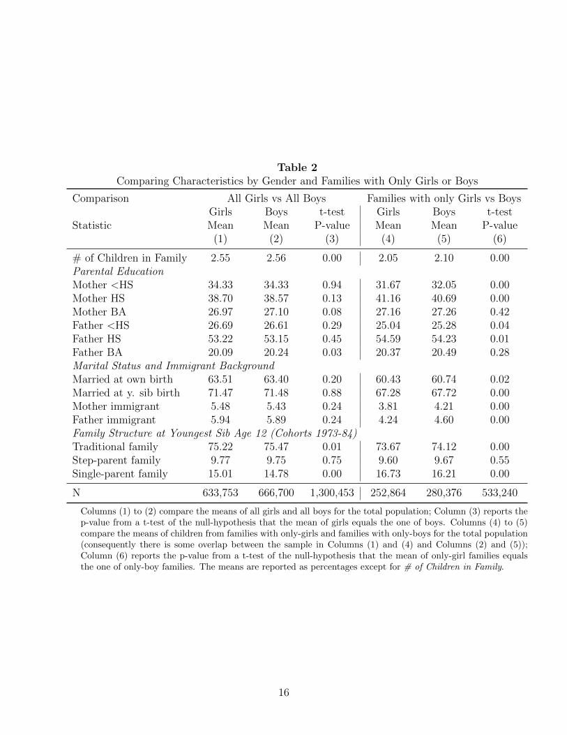
Table 2Comparing Characteristics by Gender and Families with Only Girls or Boys

Comparison All Girls vs All Boys Families with only Girls vs BoysGirls Boys t-test Girls Boys t-test

Statistic Mean Mean P-value Mean Mean P-value(1) (2) (3) (4) (5) (6)

# of Children in Family 2.55 2.56 0.00 2.05 2.10 0.00Parental EducationMother <HS 34.33 34.33 0.94 31.67 32.05 0.00Mother HS 38.70 38.57 0.13 41.16 40.69 0.00Mother BA 26.97 27.10 0.08 27.16 27.26 0.42Father <HS 26.69 26.61 0.29 25.04 25.28 0.04Father HS 53.22 53.15 0.45 54.59 54.23 0.01Father BA 20.09 20.24 0.03 20.37 20.49 0.28Marital Status and Immigrant BackgroundMarried at own birth 63.51 63.40 0.20 60.43 60.74 0.02Married at y. sib birth 71.47 71.48 0.88 67.28 67.72 0.00Mother immigrant 5.48 5.43 0.24 3.81 4.21 0.00Father immigrant 5.94 5.89 0.24 4.24 4.60 0.00Family Structure at Youngest Sib Age 12 (Cohorts 1973-84)Traditional family 75.22 75.47 0.01 73.67 74.12 0.00Step-parent family 9.77 9.75 0.75 9.60 9.67 0.55Single-parent family 15.01 14.78 0.00 16.73 16.21 0.00

N 633,753 666,700 1,300,453 252,864 280,376 533,240

Columns (1) to (2) compare the means of all girls and all boys for the total population; Column (3) reports thep-value from a t-test of the null-hypothesis that the mean of girls equals the one of boys. Columns (4) to (5)compare the means of children from families with only-girls and families with only-boys for the total population(consequently there is some overlap between the sample in Columns (1) and (4) and Columns (2) and (5));Column (6) reports the p-value from a t-test of the null-hypothesis that the mean of only-girl families equalsthe one of only-boy families. The means are reported as percentages except for # of Children in Family.

16

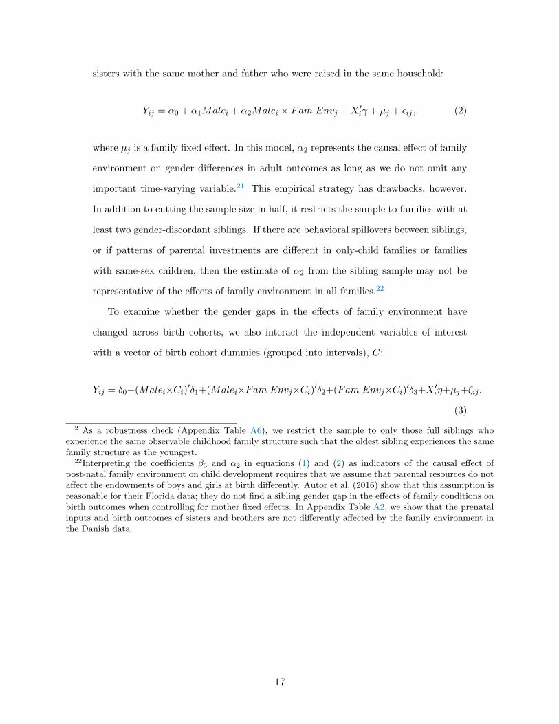
sisters with the same mother and father who were raised in the same household:

Yij = α0 + α1Malei + α2Malei × Fam Envj +X ′iγ + µj + εij , (2)

where µj is a family fixed effect. In this model, α2 represents the causal effect of family

environment on gender differences in adult outcomes as long as we do not omit any

important time-varying variable.21 This empirical strategy has drawbacks, however.

In addition to cutting the sample size in half, it restricts the sample to families with at

least two gender-discordant siblings. If there are behavioral spillovers between siblings,

or if patterns of parental investments are different in only-child families or families

with same-sex children, then the estimate of α2 from the sibling sample may not be

representative of the effects of family environment in all families.22

To examine whether the gender gaps in the effects of family environment have

changed across birth cohorts, we also interact the independent variables of interest

with a vector of birth cohort dummies (grouped into intervals), C:

Yij = δ0+(Malei×Ci)′δ1+(Malei×Fam Envj×Ci)

′δ2+(Fam Envj×Ci)′δ3+X ′iη+µj+ζij .

(3)

21As a robustness check (Appendix Table A6), we restrict the sample to only those full siblings whoexperience the same observable childhood family structure such that the oldest sibling experiences the samefamily structure as the youngest.

22Interpreting the coefficients β3 and α2 in equations (1) and (2) as indicators of the causal effect ofpost-natal family environment on child development requires that we assume that parental resources do notaffect the endowments of boys and girls at birth differently. Autor et al. (2016) show that this assumption isreasonable for their Florida data; they do not find a sibling gender gap in the effects of family conditions onbirth outcomes when controlling for mother fixed effects. In Appendix Table A2, we show that the prenatalinputs and birth outcomes of sisters and brothers are not differently affected by the family environment inthe Danish data.

17

5 Results

5.1 Outcomes in Adolescence

Table 3 reports key coefficients from the models of Grade 9 outcomes, using both the

total population and sibling samples. Column (1) shows that, for the total popula-

tion, boys are 9.2 percentage points less likely to complete grade 9 on time than girls,

conditional on year and month of birth, birth order, maternal age at birth, and family

size.23 Column (2) adds mother’s education, immigrant background, and marital status

at birth as well as interaction terms between these variables and a male dummy. Boys

benefit more from having a high educated mother (HS and BA degree) compared to

girls; the male disadvantage is reduced by 1.0 and 2.0 percentage points for boys of HS

and BA educated mothers, respectively. Males also benefit from having an immigrant

mother and from being born to married parents. Column (3) adds father’s education

and highlights one advantage of our data (i.e. that we observe fathers’ characteristics

for almost all children): the benefit of mother’s education for boys diminishes substan-

tially when father’s education is included and father’s education further reduces the

gender gap within families with better educated fathers. For highly educated fathers,

the gender gap is reduced by 2.6 percentage points (23 percent compared to children

with less than HS educated fathers). Column (4) estimates the same model as in Col-

umn (3) but on the sibling sample rather than the total population with very similar

point estimates and significance levels. Finally, Column (5) includes family fixed effects

for the sibling sample, which again give very similar results compared to using the total

population without fixed effects.

The gender gap in grade 9 GPA is large – almost 0.30 of a standard deviation [Col-

umn (6)]. The results for this outcome are somewhat different from other adolescent

outcomes in that some indicators of parental resources increase, rather than decrease,

the gender gap and there are some discrepancies between the results from the total and

23This number is 8.7 percentage points for the sibling sample without controlling for family fixed effectsand 8.9 percentage points with fixed effects, see Columns (3) and (6) in Panel A in Appendix Table A7.

18

the sibling samples. Paternal college education reduces the gender gap in grade 9 GPA

[Columns (8) to (10)]; this is true for all model versions and the effect nearly doubles

in the fixed-effect model. However, having married parents at birth increases the gap.

Maternal education and father’s HS education also increase the gender gap in the OLS

estimates, for the total population, but are insignificant in all other models. Overall,

differential gender impacts of family advantage do not explain much of the gender gap

in grade 9 achievement.

Table 4 examines sibling differences in diagnosis for behavioral and emotional dis-

order and attending special education during 9th grade. From Columns (1) and (6),

it is clear that these outcomes are more prevalent among boys: 63 percent of those

with behavioral and emotional problems and 67 percent of those attending special ed-

ucation are male. 24 The OLS models of behavioral and emotional disorder indicate

that higher parental education reduces the gender gap [Columns (2) to (4)] in the total

sample. Only father’s BA is still significant in the sibling model with fixed effects.

However, both maternal and paternal education decrease the probability of attending

special education much more for boys than girls [Columns (5) to (6)].

We observe on-time completion of grade 9 consistently across cohorts, and therefore

use this outcome to look at whether the gender gap in the effects of family environment

has changed over time. Since we examine adult outcomes as well, we want to know

whether potential varying effects between childhood and adult outcomes are due to

different ages at observation or due to different birth cohorts. For this analysis, we

estimate equation (3).

24Kristoffersen et al. (2015) find a strong association between behavioral problems and school outcomesfor Danish children, but the behavioral gender gap explains only a fraction of the gender difference in testscores.

19

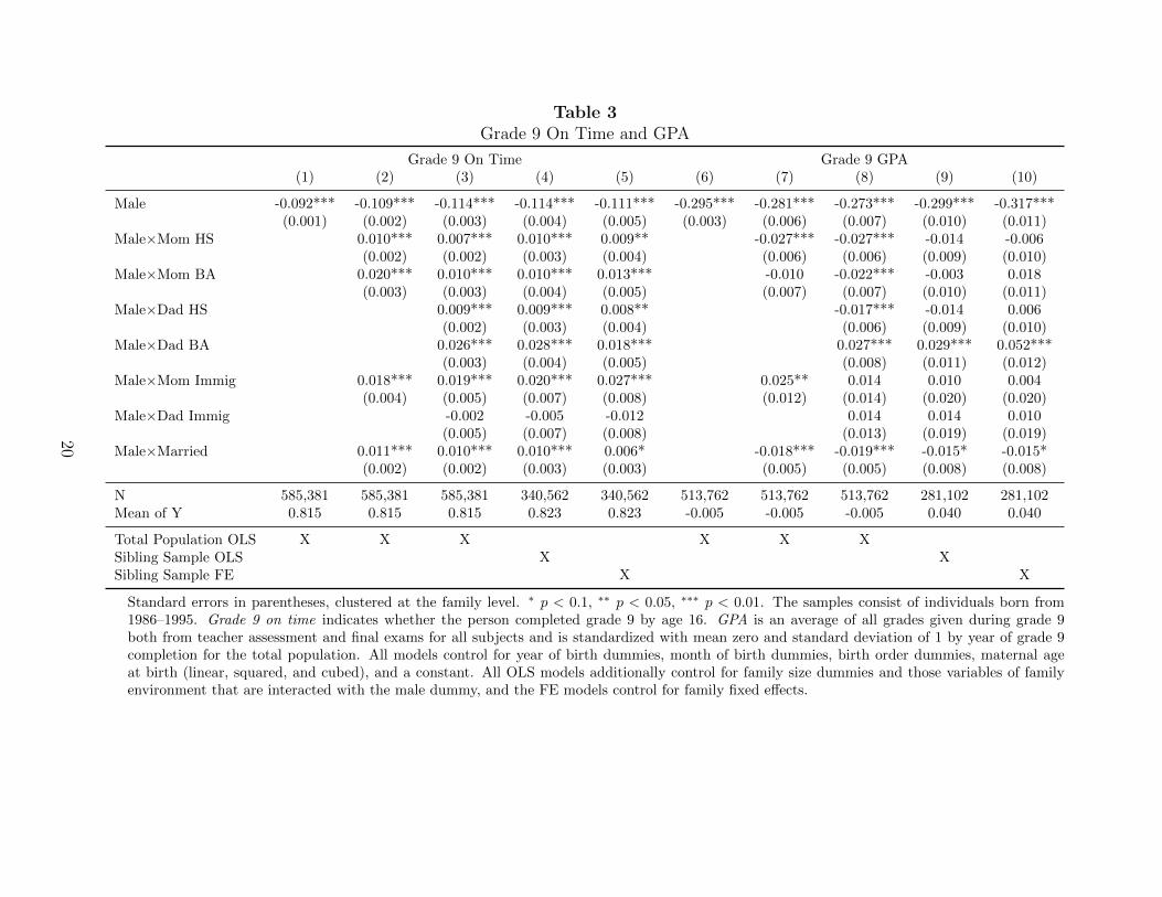
Table 3Grade 9 On Time and GPA

Grade 9 On Time Grade 9 GPA(1) (2) (3) (4) (5) (6) (7) (8) (9) (10)

Male -0.092*** -0.109*** -0.114*** -0.114*** -0.111*** -0.295*** -0.281*** -0.273*** -0.299*** -0.317***(0.001) (0.002) (0.003) (0.004) (0.005) (0.003) (0.006) (0.007) (0.010) (0.011)

Male×Mom HS 0.010*** 0.007*** 0.010*** 0.009** -0.027*** -0.027*** -0.014 -0.006(0.002) (0.002) (0.003) (0.004) (0.006) (0.006) (0.009) (0.010)

Male×Mom BA 0.020*** 0.010*** 0.010*** 0.013*** -0.010 -0.022*** -0.003 0.018(0.003) (0.003) (0.004) (0.005) (0.007) (0.007) (0.010) (0.011)

Male×Dad HS 0.009*** 0.009*** 0.008** -0.017*** -0.014 0.006(0.002) (0.003) (0.004) (0.006) (0.009) (0.010)

Male×Dad BA 0.026*** 0.028*** 0.018*** 0.027*** 0.029*** 0.052***(0.003) (0.004) (0.005) (0.008) (0.011) (0.012)

Male×Mom Immig 0.018*** 0.019*** 0.020*** 0.027*** 0.025** 0.014 0.010 0.004(0.004) (0.005) (0.007) (0.008) (0.012) (0.014) (0.020) (0.020)

Male×Dad Immig -0.002 -0.005 -0.012 0.014 0.014 0.010(0.005) (0.007) (0.008) (0.013) (0.019) (0.019)

Male×Married 0.011*** 0.010*** 0.010*** 0.006* -0.018*** -0.019*** -0.015* -0.015*(0.002) (0.002) (0.003) (0.003) (0.005) (0.005) (0.008) (0.008)

N 585,381 585,381 585,381 340,562 340,562 513,762 513,762 513,762 281,102 281,102Mean of Y 0.815 0.815 0.815 0.823 0.823 -0.005 -0.005 -0.005 0.040 0.040

Total Population OLS X X X X X XSibling Sample OLS X XSibling Sample FE X X

Standard errors in parentheses, clustered at the family level. ∗ p < 0.1, ∗∗ p < 0.05, ∗∗∗ p < 0.01. The samples consist of individuals born from1986–1995. Grade 9 on time indicates whether the person completed grade 9 by age 16. GPA is an average of all grades given during grade 9both from teacher assessment and final exams for all subjects and is standardized with mean zero and standard deviation of 1 by year of grade 9completion for the total population. All models control for year of birth dummies, month of birth dummies, birth order dummies, maternal ageat birth (linear, squared, and cubed), and a constant. All OLS models additionally control for family size dummies and those variables of familyenvironment that are interacted with the male dummy, and the FE models control for family fixed effects.

20

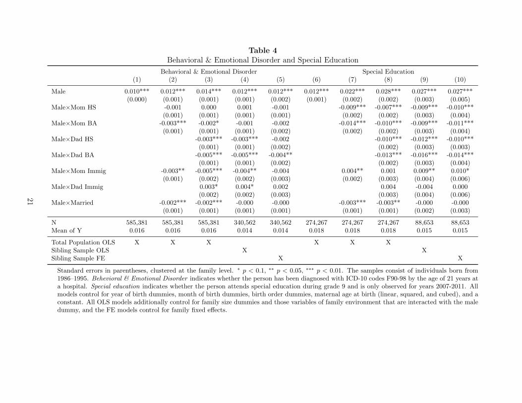
Table 4Behavioral & Emotional Disorder and Special Education

Behavioral & Emotional Disorder Special Education(1) (2) (3) (4) (5) (6) (7) (8) (9) (10)

Male 0.010*** 0.012*** 0.014*** 0.012*** 0.012*** 0.012*** 0.022*** 0.028*** 0.027*** 0.027***(0.000) (0.001) (0.001) (0.001) (0.002) (0.001) (0.002) (0.002) (0.003) (0.005)

Male×Mom HS -0.001 0.000 0.001 -0.001 -0.009*** -0.007*** -0.009*** -0.010***(0.001) (0.001) (0.001) (0.001) (0.002) (0.002) (0.003) (0.004)

Male×Mom BA -0.003*** -0.002* -0.001 -0.002 -0.014*** -0.010*** -0.009*** -0.011***(0.001) (0.001) (0.001) (0.002) (0.002) (0.002) (0.003) (0.004)

Male×Dad HS -0.003*** -0.003*** -0.002 -0.010*** -0.012*** -0.010***(0.001) (0.001) (0.002) (0.002) (0.003) (0.003)

Male×Dad BA -0.005*** -0.005*** -0.004** -0.013*** -0.016*** -0.014***(0.001) (0.001) (0.002) (0.002) (0.003) (0.004)

Male×Mom Immig -0.003** -0.005*** -0.004** -0.004 0.004** 0.001 0.009** 0.010*(0.001) (0.002) (0.002) (0.003) (0.002) (0.003) (0.004) (0.006)

Male×Dad Immig 0.003* 0.004* 0.002 0.004 -0.004 0.000(0.002) (0.002) (0.003) (0.003) (0.004) (0.006)

Male×Married -0.002*** -0.002*** -0.000 -0.000 -0.003*** -0.003** -0.000 -0.000(0.001) (0.001) (0.001) (0.001) (0.001) (0.001) (0.002) (0.003)

N 585,381 585,381 585,381 340,562 340,562 274,267 274,267 274,267 88,653 88,653Mean of Y 0.016 0.016 0.016 0.014 0.014 0.018 0.018 0.018 0.015 0.015

Total Population OLS X X X X X XSibling Sample OLS X XSibling Sample FE X X

Standard errors in parentheses, clustered at the family level. ∗ p < 0.1, ∗∗ p < 0.05, ∗∗∗ p < 0.01. The samples consist of individuals born from1986–1995. Behevioral & Emotional Disorder indicates whether the person has been diagnosed with ICD-10 codes F90-98 by the age of 21 years ata hospital. Special education indicates whether the person attends special education during grade 9 and is only observed for years 2007-2011. Allmodels control for year of birth dummies, month of birth dummies, birth order dummies, maternal age at birth (linear, squared, and cubed), and aconstant. All OLS models additionally control for family size dummies and those variables of family environment that are interacted with the maledummy, and the FE models control for family fixed effects.

21

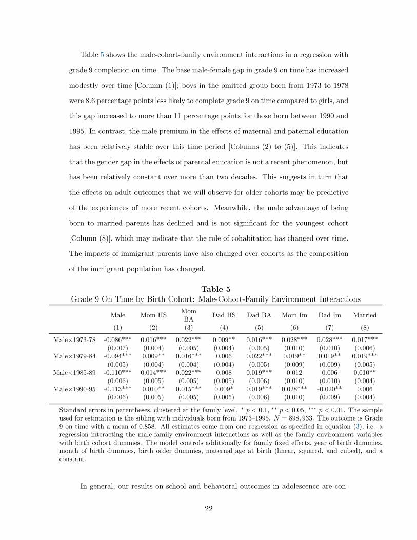
Table 5 shows the male-cohort-family environment interactions in a regression with

grade 9 completion on time. The base male-female gap in grade 9 on time has increased

modestly over time [Column (1)]; boys in the omitted group born from 1973 to 1978

were 8.6 percentage points less likely to complete grade 9 on time compared to girls, and

this gap increased to more than 11 percentage points for those born between 1990 and

1995. In contrast, the male premium in the effects of maternal and paternal education

has been relatively stable over this time period [Columns (2) to (5)]. This indicates

that the gender gap in the effects of parental education is not a recent phenomenon, but

has been relatively constant over more than two decades. This suggests in turn that

the effects on adult outcomes that we will observe for older cohorts may be predictive

of the experiences of more recent cohorts. Meanwhile, the male advantage of being

born to married parents has declined and is not significant for the youngest cohort

[Column (8)], which may indicate that the role of cohabitation has changed over time.

The impacts of immigrant parents have also changed over cohorts as the composition

of the immigrant population has changed.

Table 5Grade 9 On Time by Birth Cohort: Male-Cohort-Family Environment Interactions

Male Mom HSMomBA

Dad HS Dad BA Mom Im Dad Im Married

(1) (2) (3) (4) (5) (6) (7) (8)

Male×1973-78 -0.086*** 0.016*** 0.022*** 0.009** 0.016*** 0.028*** 0.028*** 0.017***(0.007) (0.004) (0.005) (0.004) (0.005) (0.010) (0.010) (0.006)

Male×1979-84 -0.094*** 0.009** 0.016*** 0.006 0.022*** 0.019** 0.019** 0.019***(0.005) (0.004) (0.004) (0.004) (0.005) (0.009) (0.009) (0.005)

Male×1985-89 -0.110*** 0.014*** 0.022*** 0.008 0.019*** 0.012 0.006 0.010**(0.006) (0.005) (0.005) (0.005) (0.006) (0.010) (0.010) (0.004)

Male×1990-95 -0.113*** 0.010** 0.015*** 0.009* 0.019*** 0.028*** -0.020** 0.006(0.006) (0.005) (0.005) (0.005) (0.006) (0.010) (0.009) (0.004)

Standard errors in parentheses, clustered at the family level. ∗ p < 0.1, ∗∗ p < 0.05, ∗∗∗ p < 0.01. The sampleused for estimation is the sibling with individuals born from 1973–1995. N = 898, 933. The outcome is Grade9 on time with a mean of 0.858. All estimates come from one regression as specified in equation (3), i.e. aregression interacting the male-family environment interactions as well as the family environment variableswith birth cohort dummies. The model controls additionally for family fixed effects, year of birth dummies,month of birth dummies, birth order dummies, maternal age at birth (linear, squared, and cubed), and aconstant.

In general, our results on school and behavioral outcomes in adolescence are con-

22

sistent with previous studies finding that boys benefit more from a good family back-

ground than girls in terms of outcomes indicative of learning and developmental prob-

lems (Bedard and Witman, 2015; Bertrand and Pan, 2013; Autor et al., 2016). Using

Danish data, we are able to support the overall finding for the U.S. that boys seem more

vulnerable to a disadvantageous family environment than their sisters when looking at

adolescent outcomes. Notably, we find that boys benefit differentially from high pa-

ternal education, and that the effects of parental education have been relatively stable

over time.

5.2 Adult Outcomes

When we turn to educational attainment, employment, and earnings at age 27 we find,

in contrast to school-age outcomes, that women benefit more from higher maternal ed-

ucation than men. This is true for both samples and is robust to the inclusion of family

fixed effects. For the total population, men complete less education than women with

a raw gender gap of 4.0 months [Table 6, Column (1)]. This gap is strongly increasing

in maternal education [Column (2)]. The gender gap in educational attainment rises

from 3.3 months for children of less than HS mothers to 4.6 and 6.1 months in families

with, respectively, HS and BA educated mothers [Column (3)]; these results are insen-

sitive to the inclusion of family fixed effects [Column (4)]. Paternal education, on the

other hand, seems to benefit sons more than daughters, though the effects are smaller

than those of maternal education, especially for the total population. Having a HS or

BA educated father reduces the gender gap by only about 0.6 months [Column (5)].25

Neither marital status at birth nor childhood family structure significantly affect the

gender gap in educational attainment, while having an immigrant father differentially

benefits daughters.26 Consequently, these results do not support the hypothesis that

men are more vulnerable to a disadvantageous family background than women.

25In results not reported here, we have also considered the natural logarithm of educational attainmentto examine whether we would find a similar pattern when looking at relative instead of absolute differences.Those results are in line with the ones reported here on educational attainment.

26In results not reported here, we find that this effect is limited to non-Western immigrant fathers.

23

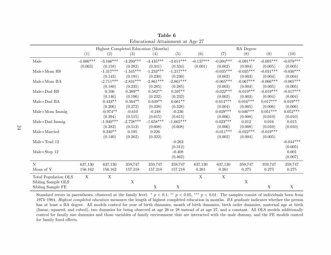
Table 6Educational Attainment at Age 27

Highest Completed Education (Months) BA Degree(1) (2) (3) (4) (5) (6) (7) (8) (9) (10)

Male -4.000*** -3.166*** -3.293*** -3.435*** -3.011*** -0.137*** -0.094*** -0.091*** -0.095*** -0.079***(0.063) (0.158) (0.282) (0.341) (0.334) (0.001) (0.002) (0.004) (0.005) (0.005)

Male×Mom HS -1.317*** -1.345*** -1.233*** -1.217*** -0.035*** -0.035*** -0.031*** -0.030***(0.143) (0.191) (0.230) (0.230) (0.002) (0.003) (0.004) (0.004)

Male×Mom BA -2.711*** -2.831*** -2.861*** -2.861*** -0.065*** -0.067*** -0.066*** -0.065***(0.180) (0.235) (0.285) (0.285) (0.003) (0.004) (0.005) (0.005)

Male×Dad HS 0.106 0.389** 0.582** 0.597** -0.022*** -0.019*** -0.019*** -0.017***(0.146) (0.196) (0.232) (0.232) (0.002) (0.003) (0.004) (0.004)

Male×Dad BA 0.433** 0.564** 0.649** 0.661** 0.014*** 0.016*** 0.017*** 0.019***(0.206) (0.272) (0.328) (0.328) (0.004) (0.005) (0.006) (0.006)

Male×Mom Immig -0.974** -0.610 -0.248 -0.236 0.029*** 0.046*** 0.051*** 0.052***(0.394) (0.515) (0.615) (0.615) (0.006) (0.008) (0.010) (0.010)

Male×Dad Immig -1.940*** -2.728*** -1.658*** -1.665*** 0.023*** 0.012 0.016 0.015(0.383) (0.513) (0.608) (0.608) (0.006) (0.008) (0.010) (0.010)

Male×Married 0.340** 0.195 0.226 -0.011*** -0.022*** -0.019***(0.140) (0.262) (0.322) (0.002) (0.004) (0.005)

Male×Trad 12 -0.263 -0.044***(0.312) (0.005)

Male×Step 12 -0.408 0.001(0.462) (0.007)

N 637,130 637,130 359,747 359,747 359,747 637,130 637,130 359,747 359,747 359,747Mean of Y 156.162 156.162 157.218 157.218 157.218 0.261 0.261 0.275 0.275 0.275

Total Population OLS X X X XSibling Sample OLS X XSibling Sample FE X X X X

Standard errors in parentheses, clustered at the family level. ∗ p < 0.1, ∗∗ p < 0.05, ∗∗∗ p < 0.01. The samples consist of individuals born from1973–1984. Highest completed education measures the length of highest completed education in months. BA graduate indicates whether the personhas at least a BA degree. All models control for year of birth dummies, month of birth dummies, birth order dummies, maternal age at birth(linear, squared, and cubed), two dummies for being observed at age 26 or 28 instead of at age 27, and a constant. All OLS models additionallycontrol for family size dummies and those variables of family environment that are interacted with the male dummy, and the FE models controlfor family fixed effects.

24

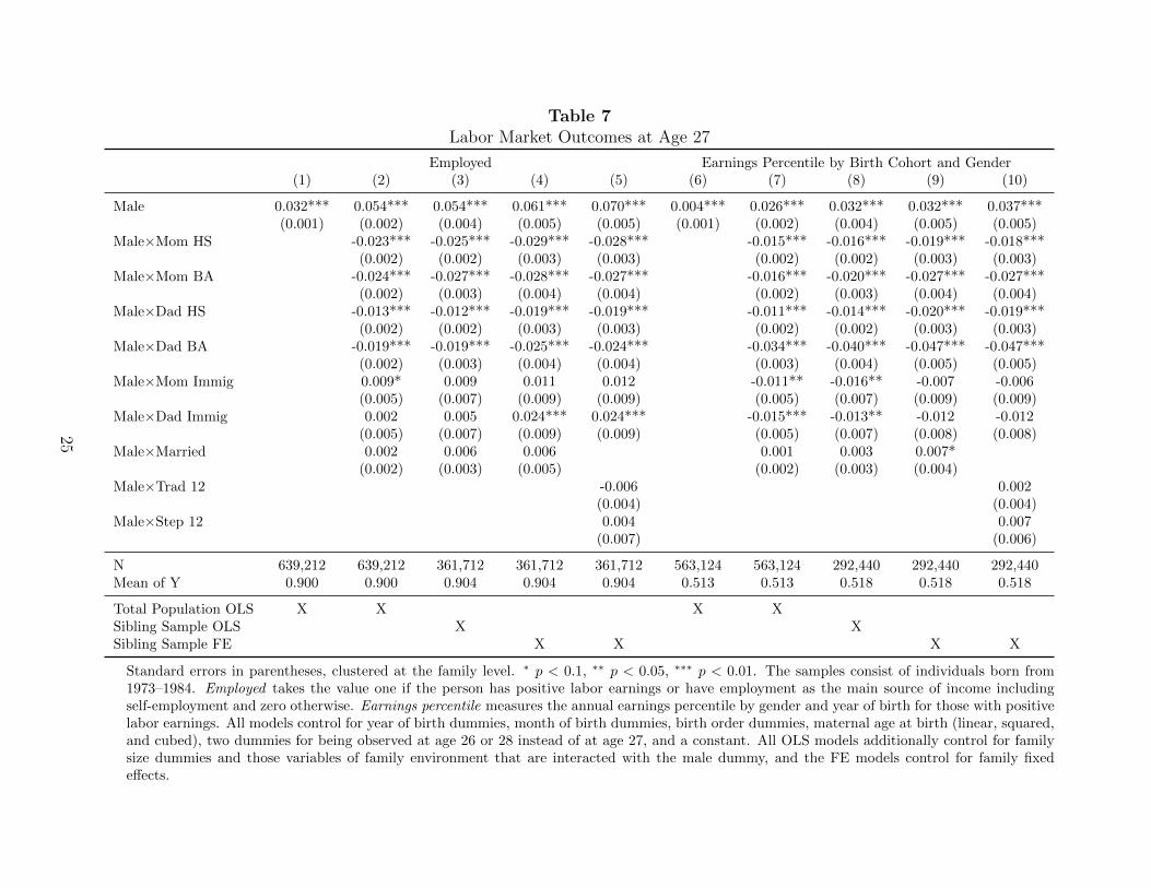
Table 7Labor Market Outcomes at Age 27

Employed Earnings Percentile by Birth Cohort and Gender(1) (2) (3) (4) (5) (6) (7) (8) (9) (10)

Male 0.032*** 0.054*** 0.054*** 0.061*** 0.070*** 0.004*** 0.026*** 0.032*** 0.032*** 0.037***(0.001) (0.002) (0.004) (0.005) (0.005) (0.001) (0.002) (0.004) (0.005) (0.005)

Male×Mom HS -0.023*** -0.025*** -0.029*** -0.028*** -0.015*** -0.016*** -0.019*** -0.018***(0.002) (0.002) (0.003) (0.003) (0.002) (0.002) (0.003) (0.003)

Male×Mom BA -0.024*** -0.027*** -0.028*** -0.027*** -0.016*** -0.020*** -0.027*** -0.027***(0.002) (0.003) (0.004) (0.004) (0.002) (0.003) (0.004) (0.004)

Male×Dad HS -0.013*** -0.012*** -0.019*** -0.019*** -0.011*** -0.014*** -0.020*** -0.019***(0.002) (0.002) (0.003) (0.003) (0.002) (0.002) (0.003) (0.003)

Male×Dad BA -0.019*** -0.019*** -0.025*** -0.024*** -0.034*** -0.040*** -0.047*** -0.047***(0.002) (0.003) (0.004) (0.004) (0.003) (0.004) (0.005) (0.005)

Male×Mom Immig 0.009* 0.009 0.011 0.012 -0.011** -0.016** -0.007 -0.006(0.005) (0.007) (0.009) (0.009) (0.005) (0.007) (0.009) (0.009)

Male×Dad Immig 0.002 0.005 0.024*** 0.024*** -0.015*** -0.013** -0.012 -0.012(0.005) (0.007) (0.009) (0.009) (0.005) (0.007) (0.008) (0.008)

Male×Married 0.002 0.006 0.006 0.001 0.003 0.007*(0.002) (0.003) (0.005) (0.002) (0.003) (0.004)

Male×Trad 12 -0.006 0.002(0.004) (0.004)

Male×Step 12 0.004 0.007(0.007) (0.006)

N 639,212 639,212 361,712 361,712 361,712 563,124 563,124 292,440 292,440 292,440Mean of Y 0.900 0.900 0.904 0.904 0.904 0.513 0.513 0.518 0.518 0.518

Total Population OLS X X X XSibling Sample OLS X XSibling Sample FE X X X X

Standard errors in parentheses, clustered at the family level. ∗ p < 0.1, ∗∗ p < 0.05, ∗∗∗ p < 0.01. The samples consist of individuals born from1973–1984. Employed takes the value one if the person has positive labor earnings or have employment as the main source of income includingself-employment and zero otherwise. Earnings percentile measures the annual earnings percentile by gender and year of birth for those with positivelabor earnings. All models control for year of birth dummies, month of birth dummies, birth order dummies, maternal age at birth (linear, squared,and cubed), two dummies for being observed at age 26 or 28 instead of at age 27, and a constant. All OLS models additionally control for familysize dummies and those variables of family environment that are interacted with the male dummy, and the FE models control for family fixedeffects.

25

Turning to the binary outcome of having received a BA degree by age 27, we find

results quite similar to those in the educational attainment model, with two exceptions.

First, women of HS educated fathers benefit more than their brothers, though boys

benefit more from a college-educated father. Second, women also benefit more than

their brothers from having parents who were married when they were born [Columns

(7) to (9)] and living in a traditional family during childhood [Column (10)]. These

results are sharply at odds with those we saw for school outcomes at age 16: on most

dimensions, women benefit more from a favorable childhood family environment than

their brothers in terms of higher educational attainment in adulthood.

Table 7 presents results for labor market outcomes at age 27. Column 1 shows that

men are 3.2 percentage points more likely to be employed than women. However, we

again see the pattern that women benefit more than their brothers from having parents

with at least HS education, with effects of maternal and paternal education that are

significant and of similar magnitudes. The employment gap is larger for families with an

immigrant father when comparing sisters and brothers in fixed effects models [Columns

(4) and (5)], which may be a reflection of more traditional gender norms.27

For individuals with positive labor earnings, parental education differentially in-

creases the earnings percentile of women relative to their brothers. Women whose

parents have at least a HS degree earn more than their brothers relative to their birth

cohort and gender, and the effect of paternal college education is particularly strong

(4.7 percentage points). We find no gender gap in the effects of childhood family struc-

ture on either employment or earnings except for a small borderline significant effect

on earnings (favoring boys) of married parents at birth.

5.3 Adult Outcomes Across Cohorts

We have found that women consistently benefit more from high maternal education

than their brothers in terms of educational attainment and labor market outcomes at

age 27. In this section, we examine whether these gender differences in the effects of

27The immigrant effect is limited to families in which one or both parents is of non-Western origin.

26

parental education have changed across cohorts.

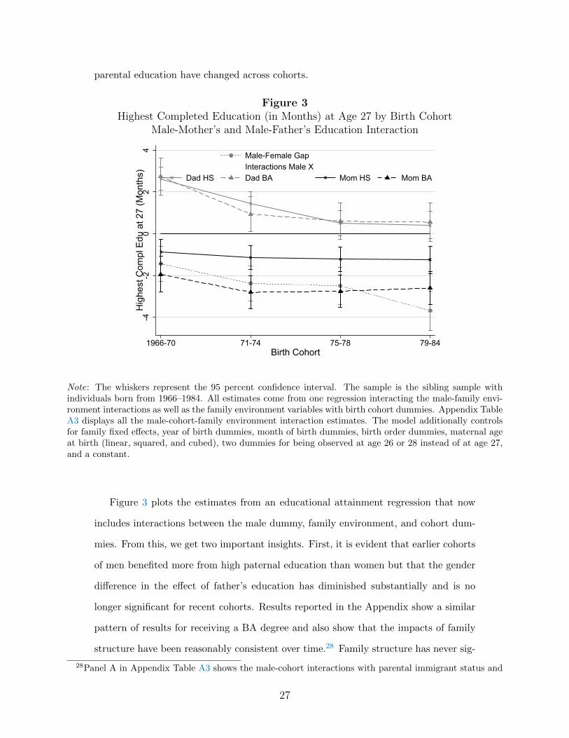
Figure 3Highest Completed Education (in Months) at Age 27 by Birth Cohort

Male-Mother’s and Male-Father’s Education Interaction

-4-2

02

4H

ighe

st C

ompl

Edu

at 2

7 (M

onth

s)

1966-70 71-74 75-78 79-84Birth Cohort

Male-Female Gap Interactions Male X Dad HS Dad BA Mom HS Mom BA

Note: The whiskers represent the 95 percent confidence interval. The sample is the sibling sample withindividuals born from 1966–1984. All estimates come from one regression interacting the male-family envi-ronment interactions as well as the family environment variables with birth cohort dummies. Appendix TableA3 displays all the male-cohort-family environment interaction estimates. The model additionally controlsfor family fixed effects, year of birth dummies, month of birth dummies, birth order dummies, maternal ageat birth (linear, squared, and cubed), two dummies for being observed at age 26 or 28 instead of at age 27,and a constant.

Figure 3 plots the estimates from an educational attainment regression that now

includes interactions between the male dummy, family environment, and cohort dum-

mies. From this, we get two important insights. First, it is evident that earlier cohorts

of men benefited more from high paternal education than women but that the gender

difference in the effect of father’s education has diminished substantially and is no

longer significant for recent cohorts. Results reported in the Appendix show a similar

pattern of results for receiving a BA degree and also show that the impacts of family

structure have been reasonably consistent over time.28 Family structure has never sig-

28Panel A in Appendix Table A3 shows the male-cohort interactions with parental immigrant status and

27

nificantly affected the gender gap in educational attainment, though living in a stable

family during childhood has consistently favored women for all cohorts in terms of the

likelihood of receiving a BA. Consequently, this evidence does not support the hypoth-

esis that the increasing prevalence of non-traditional family arrangements explain the

growing education gap in favor of girls.

Finally, Table 8 examines whether the gender gap in the effects of childhood family

environment on labor market outcomes has changed across cohorts (1973–1978 vs 1966–

1971) and how they vary across ages (27, 33, and 40). The raw employment gap

between men and women narrows as they age such that men in the older cohort are

only 1.9 percentage points more likely to be employed than women at age 40, compared

to a gap of 5.0 percentage points at age 27 [Columns (3) and (5), Panel A]. The

gender differences in the effects of parental education on employment at the same age

are similar across cohorts though, as siblings age, the differential impact of parental

education on men and women in employment falls and has essentially disappeared by

age 40.

The age pattern of parental education effects on the earnings percentile is different.

At age 27, both maternal and paternal education have more positive effects on women’s

earnings. By age 40, maternal education no longer has a differential effect on sons and

daughters, and paternal education has a stronger impact on sons. This change may

reflect the different career lifecycles of men and women, especially related to childbirth

(Kleven et al. (2015)).

childhood family structure from this model. The impacts of immigrant parents have changed across cohorts,perhaps as a consequence of changing composition of this group. The results in Figure 3 are basicallyidentical when only considering traditional families. Though we do not report the results here, if we excludethe male-paternal education interactions, the gender gap in the effects of maternal education appear to beincreasing over time, indicating a spurious trend in the impact of mother’s education.

28

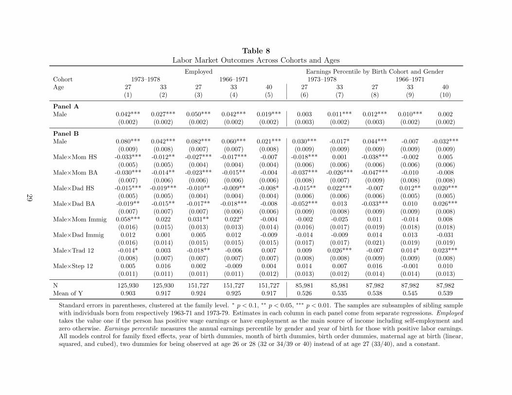
Table 8Labor Market Outcomes Across Cohorts and Ages

Employed Earnings Percentile by Birth Cohort and GenderCohort 1973–1978 1966–1971 1973–1978 1966–1971Age 27 33 27 33 40 27 33 27 33 40

(1) (2) (3) (4) (5) (6) (7) (8) (9) (10)

Panel AMale 0.042*** 0.027*** 0.050*** 0.042*** 0.019*** 0.003 0.011*** 0.012*** 0.010*** 0.002

(0.002) (0.002) (0.002) (0.002) (0.002) (0.003) (0.002) (0.003) (0.002) (0.002)

Panel BMale 0.080*** 0.042*** 0.082*** 0.060*** 0.021*** 0.030*** -0.017* 0.044*** -0.007 -0.032***

(0.009) (0.008) (0.007) (0.007) (0.008) (0.009) (0.009) (0.009) (0.009) (0.009)Male×Mom HS -0.033*** -0.012** -0.027*** -0.017*** -0.007 -0.018*** 0.001 -0.038*** -0.002 0.005

(0.005) (0.005) (0.004) (0.004) (0.004) (0.006) (0.006) (0.006) (0.006) (0.006)Male×Mom BA -0.030*** -0.014** -0.023*** -0.015** -0.004 -0.037*** -0.026*** -0.047*** -0.010 -0.008

(0.007) (0.006) (0.006) (0.006) (0.006) (0.008) (0.007) (0.009) (0.008) (0.008)Male×Dad HS -0.015*** -0.019*** -0.010** -0.009** -0.008* -0.015** 0.022*** -0.007 0.012** 0.020***

(0.005) (0.005) (0.004) (0.004) (0.004) (0.006) (0.006) (0.006) (0.005) (0.005)Male×Dad BA -0.019** -0.015** -0.017** -0.018*** -0.008 -0.052*** 0.013 -0.033*** 0.010 0.026***

(0.007) (0.007) (0.007) (0.006) (0.006) (0.009) (0.008) (0.009) (0.009) (0.008)Male×Mom Immig 0.058*** 0.022 0.031** 0.022* -0.004 -0.002 -0.025 0.011 -0.014 0.008

(0.016) (0.015) (0.013) (0.013) (0.014) (0.016) (0.017) (0.019) (0.018) (0.018)Male×Dad Immig 0.012 0.001 0.005 0.012 -0.009 -0.014 -0.009 0.014 0.013 -0.031

(0.016) (0.014) (0.015) (0.015) (0.015) (0.017) (0.017) (0.021) (0.019) (0.019)Male×Trad 12 -0.014* 0.003 -0.018** -0.006 0.007 0.009 0.026*** -0.007 0.014* 0.023***

(0.008) (0.007) (0.007) (0.007) (0.007) (0.008) (0.008) (0.009) (0.009) (0.008)Male×Step 12 0.005 0.016 0.002 -0.009 0.004 0.014 0.007 0.016 -0.001 0.010

(0.011) (0.011) (0.011) (0.011) (0.012) (0.013) (0.012) (0.014) (0.014) (0.013)

N 125,930 125,930 151,727 151,727 151,727 85,981 85,981 87,982 87,982 87,982Mean of Y 0.903 0.917 0.924 0.925 0.917 0.526 0.535 0.538 0.545 0.539

Standard errors in parentheses, clustered at the family level. ∗ p < 0.1, ∗∗ p < 0.05, ∗∗∗ p < 0.01. The samples are subsamples of sibling samplewith individuals born from respectively 1963-71 and 1973-79. Estimates in each column in each panel come from separate regressions. Employedtakes the value one if the person has positive wage earnings or have employment as the main source of income including self-employment andzero otherwise. Earnings percentile measures the annual earnings percentile by gender and year of birth for those with positive labor earnings.All models control for family fixed effects, year of birth dummies, month of birth dummies, birth order dummies, maternal age at birth (linear,squared, and cubed), two dummies for being observed at age 26 or 28 (32 or 34/39 or 40) instead of at age 27 (33/40), and a constant.

29

The results in this section show that gender differences in the effects of parental

education have been fairly constant across cohorts in terms of educational attainment,

with the exception that the differentially positive effect of father’s education on boys

has decreased over time. The same is true of labor market outcomes: the gender

specific responses to childhood family environment have been consistent across cohorts,

though the more positive effects of both maternal and paternal education on women’s

employment and earnings tends to diminish with age.

5.4 Sensitivity Analyses

In this subsection, we study the robustness of our findings in three different ways.

First, we examine whether different aspects of childhood family environment interact in

important ways by gender. Second, we check the robustness of our measure of childhood

family structure. Since the main results were quite similar for the different models,

we perform these two robustness analyses on the sibling sample including family fixed

effects. Third, we compare our main results (estimated on the total population and

the sibling sample) to the estimated effects for one-child families and subsamples of the

sibling sample divided by the gender composition of the siblings in the sample without

family fixed effects.

Appendix Table A4 includes interactions between mother’s and father’s education

in several key models of school and adult outcomes.29 We find some heterogeneity in

the effects of parents’ education on educational attainment at age 27.30 The results

suggest that in families where the mother has at least HS education, men do not benefit

differently than their sisters from father’s HS education in terms of highest completed

education. For college graduation, the excess female advantage from parental BA edu-

cation is smaller in families where both parents have at least HS education. Appendix

Table A5 expands the main model by interacting the family environment-male inter-

29The correlation between mother’s and father’s length of education is around 0.40 and approximately 50percent of parents have the same educational level.

30Formally, we test this with an F-test of whether the additional Male×Mom Edu×Dad Edu interactionterms are jointly equal to zero.

30

actions with marital status at birth, but we find little evidence of heterogeneity.

Appendix Table A6 tests the sensitivity of our definition of childhood family struc-

ture for the sibling sample, which is based on the experience of the youngest sibling.

Column (1) (and every second column) uses family structure defined for the oldest

sibling instead; the results are very robust to this change in our measure of childhood

family structure. In Column (2) (and every second column), we restrict the sample

to those families with children with the same observed family structure at age 12; the

results are again very similar to the main results.

Finally, Appendix Tables A7 and A8 compare OLS models of key outcomes for

alternative samples—the total population, children from one-child families, and the

sample of full siblings (which we also split by gender composition for the OLS esti-

mations [Columns (4) and (5)]). Overall, the estimates for the different subsamples

and for the total population and the sibling sample without fixed effects are similar

(both in terms of magnitude and significance), though fewer estimates are significant

in smaller samples.

6 Conclusion

Motivated by previous findings showing that school-aged boys appear more vulnerable

to family disadvantage than school-aged girls, we examine whether such differences

persist into adulthood. We use Danish administrative register data, allowing us to

examine a broad range of school and adult outcomes for complete cohorts, as well as

large samples of full siblings. An advantage compared to previous studies is that we

observe both mother’s and father’s education as well as family structure at birth and

during childhood.

In line with findings from the U.S. (Autor et al., 2016; Lundberg, 2016), we first

show that in the Danish context boys also appear to be generally more sensitive than

girls to family environment in terms of observable outcomes during school. We find

the opposite for adult outcomes, including educational attainment, college graduation,

31

employment, and earnings. Women consistently benefit more from maternal education

relative to their brothers in terms of education and employment. Paternal education

decreases the gender gap in education (favoring sons), though the impact is small. In

contrast, paternal education has larger positive effects on the employment and earn-

ings of daughters. A gender gap in the effects of family structure only exists for college

graduation and favors women. Similar results in OLS models using the entire popula-

tion and family fixed-effect models using a sample of full siblings indicate that selection

of boys and girls across family types is not a serious source of bias.

Moreover, we show the gender gap in the effects of parental education on complet-

ing grade 9 on time has been relatively constant over more than two decades. This

indicates that the gender difference in the effects of maternal education on primary

school completion is not a recent phenomenon. In terms of educational attainment

in adulthood, we find that men used to benefit more from paternal education than

women but that the gender difference in the effect of father’s education disappeared

for cohorts born after the mid-1970s. The female premium in the effects of mother’s

education has been constant for all cohorts.

Although boys respond differently to parental resources and family structure than

do girls, the evidence shows that such gender differences do not conform to the simple

story that the skill development of boys is particularly sensitive to family environ-

ment. Neither can the changes in family structure, in the Danish context, explain the

growing education gap in favor of girls. Our findings are compatible with a story in

which parental education and other family resources have a strong moderating effect

on behavioral problems in school that are much more typical of boys than girls. These

controlling forces may become less effective as the children become adults, and the

results show no indication that long-term skill acquisition, and therefore educational

attainment or adult earnings, is affected. These results fail to support a particular

targeting of boys in programs designed to assist students from disadvantaged families.

32

Acknowledgements

We are thankful for helpful comments and suggestions from Edward Samuel Jones,

Torben Heien Nielsen, Hans Henrik Sievertsen, Dick Startz, and Miriam Wust, as well

as seminar participants at University of California, Santa Barbara, at the DAEiNA

conference at Aarhus University, and at the Copenhagen Education Network Workshop.

Funding Sources

This research did not receive any specific grant from funding agencies in the public,

commercial, or not-for-profit sectors.

References

Almond, D. and L. Edlund (2007). Trivers–willard at birth and one year: evidence

from us natality data 1983–2001. Proceedings of the Royal Society of London B:

Biological Sciences 274 (1624), 2491–2496.

Autor, D., D. Figlio, K. Karbownik, J. Roth, and M. Wasserman (2016). Family

disadvantage and the gender gap in behavioral and educational outcomes. NBER

Working Paper Series.

Autor, D. and M. Wasserman (2013). Wayward sons: The emerging gender gap in

labor markets and education. Third Way Report 20013.

Baker, M. and K. Milligan (2013). Boy-girl differences in parental time investments:

Evidence from three countries. NBER Working Paper Series.

Becker, G. S., W. H. Hubbard, and K. M. Murphy (2010). Explaining the worldwide

boom in higher education of women. Journal of Human Capital 4 (3), 203–241.

Bedard, K. and A. Witman (2015). Family structure and the gender gap in adhd.

33

Bertrand, M. and J. Pan (2013). The trouble with boys: Social influences and the

gender gap in disruptive behavior. American Economic Journal: Applied Eco-

nomics 5 (1), 32–64.

Dahl, G. B. and E. Moretti (2008). The demand for sons. The Review of Economic

Studies 75 (4), 1085–1120.

Dee, T. S. and H. H. Sievertsen (2015). The gift of time? school starting age and

mental health. NBER Working Paper Series.

DiPrete, T. A. and C. Buchmann (2013). The rise of women: The growing gender gap

in education and what it means for American schools. Russell Sage Foundation.

DiPrete, T. A. and J. L. Jennings (2012). Social and behavioral skills and the gender

gap in early educational achievement. Social Science Research 41 (1), 1–15.

Duckworth, A. L. and M. E. Seligman (2006). Self-discipline gives girls the edge:

Gender in self-discipline, grades, and achievement test scores. Journal of educational

psychology 98 (1), 198.

Duncan, G. J. and K. Magnuson (2011). The nature and impact of early achievement

skills, attention skills, and behavior problems. Whither opportunity , 47–70.

Fan, X., H. Fang, and S. Markussen (2015). Mothers’ employment and children’s

educational gender gap. NBER Working Paper Series.

Fortin, N. M., P. Oreopoulos, and S. Phipps (2015). Leaving boys behind gender

disparities in high academic achievement. Journal of Human Resources 50 (3), 549–

579.

Goldin, C., L. F. Katz, and I. Kuziemko (2006). The homecoming of american college

women: The reversal of the college gender gap. NBER Working Paper Series.

Hamoudi, A. and J. Nobles (2014). Do daughters really cause divorce? stress, preg-

nancy, and family composition. Demography 51 (4), 1423–1449.

34

Kleven, H. J., C. Landais, and J. E. Søgaard (2015). Parenthood and the gender gap:

Evidence from denmark.

Kristoffersen, J. H., C. Obel, and N. Smith (2015). Gender differences in behavioral

problems and school outcomes. Journal of Economic Behavior & Organization 115,

75–93.

Landersø, R. and J. J. Heckman (2016). The scandinavian fantasy: The sources of in-

tergenerational mobility in denmark and the us. IZA Discussion Paper, forthcoming

in the Scandinavian Journal of Economics.

Lundberg, S. (2005). Sons, daughters, and parental behaviour. Oxford Review of

Economic Policy 21 (3), 340–356.

Lundberg, S. (2016). Father absence and the gender gap in college graduation.

Lundberg, S. and E. Rose (2003). Child gender and the transition to marriage. De-

mography 40 (2), 333–349.

Norberg, K. (2004). Partnership status and the human sex ratio at birth. Proceedings

of the Royal Society of London B: Biological Sciences 271 (1555), 2403–2410.

Obel, C., J. L. Zhu, J. Olsen, S. Breining, J. Li, T. K. Grønborg, M. Gissler, and

M. Rutter (2015). The risk of attention deficit hyperactivity disorder in children ex-

posed to maternal smoking during pregnancy–a reexamination using a sibling design.

Journal of Child Psychology and Psychiatry .

OECD (2015). The abc of gender equality in education.

Riphahn, R. T. and C. Schwientek (2015). What drives the reversal of the gender

education gap? evidence from germany. Applied Economics 47 (53), 5748–5775.

Rossin-Slater, M. and M. Wust (2014). Child support obligations and family outcomes:

Causal evidence from administrative data. SFI The Danish National Centre For

Social Research.

35

Simonsen, M., H. S. Nielsen, and R. Landersø (2015). School starting age and the

crime-age profile. Economic Journal .

Trivers, R. L. and D. E. Willard (1973). Natural selection of parental ability to vary

the sex ratio of offspring. Science 179 (4068), 90–92.

U.S. Census Bureau (2015). Cps historical time series tables.

36

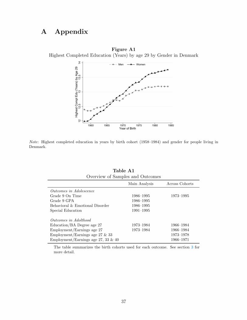
A Appendix

Figure A1Highest Completed Education (Years) by age 29 by Gender in Denmark

1212

.513

13.5

14H

ighe

st C

ompl

Edu

(Yea

rs) b

y A

ge 2

9

1960 1965 1970 1975 1980 1985Year of Birth

Men Women

Note: Highest completed education in years by birth cohort (1958–1984) and gender for people living inDenmark.

Table A1Overview of Samples and Outcomes

Main Analysis Across Cohorts

Outcomes in AdolescenceGrade 9 On Time 1986–1995 1973–1995Grade 9 GPA 1986–1995Behavioral & Emotional Disorder 1986–1995Special Education 1991–1995

Outcomes in AdolthoodEducation/BA Degree age 27 1973–1984 1966–1984Employment/Earnings age 27 1973–1984 1966–1984Employment/Earnings age 27 & 33 1973–1978Employment/Earnings age 27, 33 & 40 1966–1971

The table summarizes the birth cohorts used for each outcome. See section 3 formore detail.

37

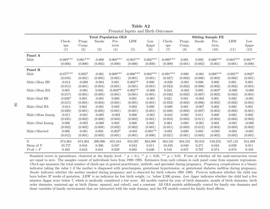
Table A2Prenatal Inputs and Birth Outcomes

Total Population OLS Sibling Sample FECheck- Pregn. Smoke Pre- LBW Low Check- Pregn. Smoke Pre- LBW Low

ups Comp. term Apgar ups Comp. term Apgar(1) (2) (3) (4) (5) (6) (7) (8) (9) (10) (11) (12)

Panel AMale -0.093*** 0.001*** -0.000 0.008*** -0.004*** 0.002*** -0.080*** 0.001 0.003 0.006*** -0.004*** 0.001**

(0.006) (0.000) (0.002) (0.000) (0.000) (0.000) (0.009) (0.001) (0.002) (0.001) (0.001) (0.000)

Panel BMale -0.077*** 0.002* -0.001 0.009*** -0.006*** 0.002*** -0.091*** 0.000 -0.001 0.008*** -0.005** 0.002*

(0.016) (0.001) (0.005) (0.001) (0.001) (0.001) (0.027) (0.002) (0.006) (0.002) (0.002) (0.001)Male×Mom HS -0.014 -0.000 -0.004 0.001 0.003** 0.000 -0.020 -0.001 0.006 0.000 0.001 0.001

(0.015) (0.001) (0.004) (0.001) (0.001) (0.001) (0.023) (0.002) (0.006) (0.002) (0.002) (0.001)Male×Mom BA 0.005 -0.001 0.002 -0.003** 0.002** -0.000 0.023 -0.002 0.005 -0.003* -0.000 -0.000

(0.017) (0.001) (0.005) (0.001) (0.001) (0.001) (0.026) (0.002) (0.007) (0.002) (0.002) (0.001)Male×Dad HS -0.026* 0.001 -0.001 0.000 0.001 -0.001 0.021 0.001 -0.003 0.001 0.002 -0.001

(0.015) (0.001) (0.004) (0.001) (0.001) (0.001) (0.023) (0.002) (0.006) (0.002) (0.002) (0.001)Male×Dad BA -0.014 0.001 -0.001 0.002 0.002 0.000 -0.008 0.001 -0.007 0.002 0.002 0.001

(0.020) (0.001) (0.005) (0.001) (0.001) (0.001) (0.030) (0.002) (0.007) (0.002) (0.002) (0.001)Male×Mom Immig -0.011 -0.001 -0.005 -0.003 0.000 -0.001 -0.044 0.002 0.011 0.000 0.002 0.002

(0.035) (0.002) (0.008) (0.003) (0.002) (0.001) (0.053) (0.003) (0.011) (0.004) (0.004) (0.002)Male×Dad Immig 0.006 -0.002 -0.000 0.002 0.000 0.002 0.064 0.000 -0.001 0.002 -0.001 -0.000

(0.032) (0.002) (0.008) (0.002) (0.002) (0.001) (0.051) (0.003) (0.012) (0.004) (0.003) (0.002)Male×Married 0.008 -0.001 0.004 -0.002* -0.001 -0.001** -0.001 0.000 0.004 -0.003 -0.001 -0.001

(0.012) (0.001) (0.003) (0.001) (0.001) (0.000) (0.021) (0.001) (0.005) (0.002) (0.002) (0.001)

N 874,364 874,364 290,990 855,344 853,207 864,998 564,531 564,531 95,853 549,252 547,131 554,489Mean of Y 10.757 0.044 0.306 0.047 0.043 0.011 10.835 0.040 0.271 0.043 0.039 0.011Prob > F 0.483 0.643 0.641 0.029 0.092 0.626 0.516 0.857 0.707 0.374 0.874 0.458

Standard errors in parentheses, clustered at the family level. ∗ p < 0.1, ∗∗ p < 0.05, ∗∗∗ p < 0.01. F-test of whether all the male-interaction termsare equal to zero. The samples consist of individuals born from 1980–1995. Estimates from each column in each panel come from separate regressions.Check-ups measures the total number of check-ups at general practitioner, midwife, and specialist during pregnancy. Pregnancy complications is a binaryindicator taking the value 1 if the mother is diagnosed with preeclampsia, gestational hypertension, or gestational diabetes mellitus during pregnancy.Smoke indicates whether the mother smoked during pregnancy and is observed for birth cohorts 1991–1995. Preterm indicates whether the child wasborn before 37 weeks of gestation. LBW is an indicator for low birth weight, i.e. below 2,500 grams. Low Apgar indicates whether the child had a fiveminutes Apgar score below 7, which is medically considered a low score. All models control for year of birth dummies, month of birth dummies, birthorder dummies, maternal age at birth (linear, squared, and cubed), and a constant. All OLS models additionally control for family size dummies andthose variables of family environment that are interacted with the male dummy, and the FE models control for family fixed effects.

38

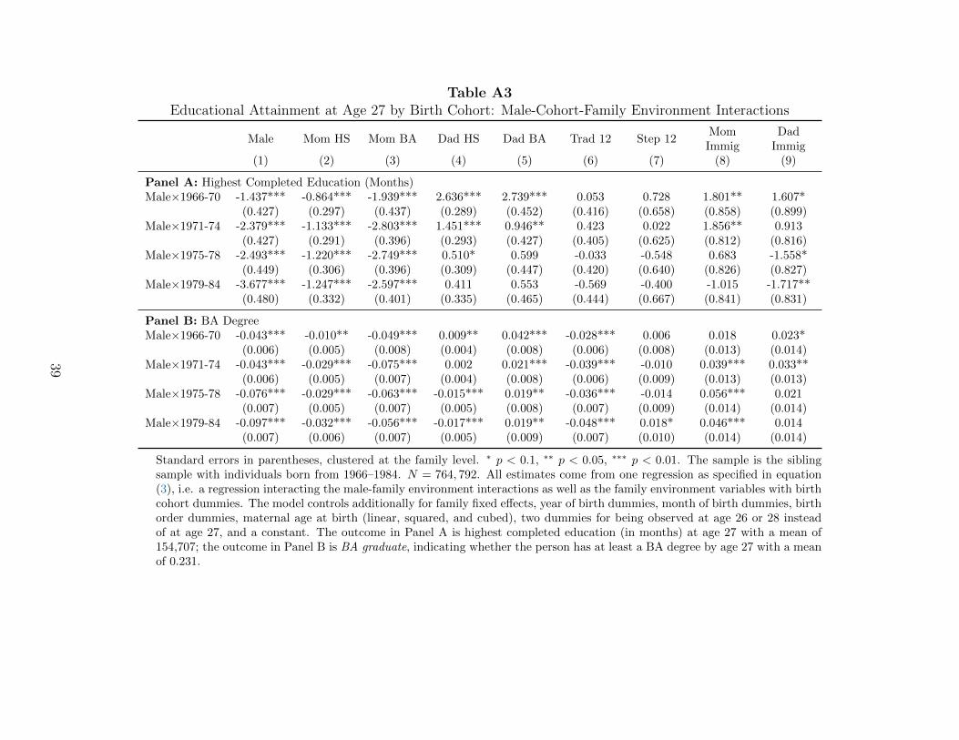
Table A3Educational Attainment at Age 27 by Birth Cohort: Male-Cohort-Family Environment Interactions

Male Mom HS Mom BA Dad HS Dad BA Trad 12 Step 12MomImmig

DadImmig

(1) (2) (3) (4) (5) (6) (7) (8) (9)

Panel A: Highest Completed Education (Months)Male×1966-70 -1.437*** -0.864*** -1.939*** 2.636*** 2.739*** 0.053 0.728 1.801** 1.607*

(0.427) (0.297) (0.437) (0.289) (0.452) (0.416) (0.658) (0.858) (0.899)Male×1971-74 -2.379*** -1.133*** -2.803*** 1.451*** 0.946** 0.423 0.022 1.856** 0.913

(0.427) (0.291) (0.396) (0.293) (0.427) (0.405) (0.625) (0.812) (0.816)Male×1975-78 -2.493*** -1.220*** -2.749*** 0.510* 0.599 -0.033 -0.548 0.683 -1.558*

(0.449) (0.306) (0.396) (0.309) (0.447) (0.420) (0.640) (0.826) (0.827)Male×1979-84 -3.677*** -1.247*** -2.597*** 0.411 0.553 -0.569 -0.400 -1.015 -1.717**

(0.480) (0.332) (0.401) (0.335) (0.465) (0.444) (0.667) (0.841) (0.831)

Panel B: BA DegreeMale×1966-70 -0.043*** -0.010** -0.049*** 0.009** 0.042*** -0.028*** 0.006 0.018 0.023*

(0.006) (0.005) (0.008) (0.004) (0.008) (0.006) (0.008) (0.013) (0.014)Male×1971-74 -0.043*** -0.029*** -0.075*** 0.002 0.021*** -0.039*** -0.010 0.039*** 0.033**

(0.006) (0.005) (0.007) (0.004) (0.008) (0.006) (0.009) (0.013) (0.013)Male×1975-78 -0.076*** -0.029*** -0.063*** -0.015*** 0.019** -0.036*** -0.014 0.056*** 0.021

(0.007) (0.005) (0.007) (0.005) (0.008) (0.007) (0.009) (0.014) (0.014)Male×1979-84 -0.097*** -0.032*** -0.056*** -0.017*** 0.019** -0.048*** 0.018* 0.046*** 0.014

(0.007) (0.006) (0.007) (0.005) (0.009) (0.007) (0.010) (0.014) (0.014)

Standard errors in parentheses, clustered at the family level. ∗ p < 0.1, ∗∗ p < 0.05, ∗∗∗ p < 0.01. The sample is the siblingsample with individuals born from 1966–1984. N = 764, 792. All estimates come from one regression as specified in equation(3), i.e. a regression interacting the male-family environment interactions as well as the family environment variables with birthcohort dummies. The model controls additionally for family fixed effects, year of birth dummies, month of birth dummies, birthorder dummies, maternal age at birth (linear, squared, and cubed), two dummies for being observed at age 26 or 28 insteadof at age 27, and a constant. The outcome in Panel A is highest completed education (in months) at age 27 with a mean of154,707; the outcome in Panel B is BA graduate, indicating whether the person has at least a BA degree by age 27 with a meanof 0.231.

39

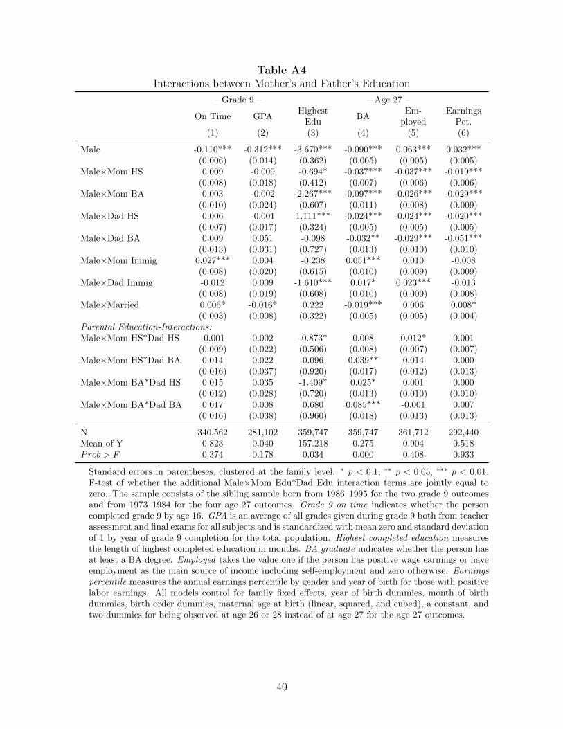
Table A4Interactions between Mother’s and Father’s Education

– Grade 9 – – Age 27 –

On Time GPAHighest

EduBA

Em-ployed

EarningsPct.

(1) (2) (3) (4) (5) (6)

Male -0.110*** -0.312*** -3.670*** -0.090*** 0.063*** 0.032***(0.006) (0.014) (0.362) (0.005) (0.005) (0.005)

Male×Mom HS 0.009 -0.009 -0.694* -0.037*** -0.037*** -0.019***(0.008) (0.018) (0.412) (0.007) (0.006) (0.006)

Male×Mom BA 0.003 -0.002 -2.267*** -0.097*** -0.026*** -0.029***(0.010) (0.024) (0.607) (0.011) (0.008) (0.009)

Male×Dad HS 0.006 -0.001 1.111*** -0.024*** -0.024*** -0.020***(0.007) (0.017) (0.324) (0.005) (0.005) (0.005)

Male×Dad BA 0.009 0.051 -0.098 -0.032** -0.029*** -0.051***(0.013) (0.031) (0.727) (0.013) (0.010) (0.010)

Male×Mom Immig 0.027*** 0.004 -0.238 0.051*** 0.010 -0.008(0.008) (0.020) (0.615) (0.010) (0.009) (0.009)

Male×Dad Immig -0.012 0.009 -1.610*** 0.017* 0.023*** -0.013(0.008) (0.019) (0.608) (0.010) (0.009) (0.008)

Male×Married 0.006* -0.016* 0.222 -0.019*** 0.006 0.008*(0.003) (0.008) (0.322) (0.005) (0.005) (0.004)

Parental Education-Interactions:Male×Mom HS*Dad HS -0.001 0.002 -0.873* 0.008 0.012* 0.001

(0.009) (0.022) (0.506) (0.008) (0.007) (0.007)Male×Mom HS*Dad BA 0.014 0.022 0.096 0.039** 0.014 0.000

(0.016) (0.037) (0.920) (0.017) (0.012) (0.013)Male×Mom BA*Dad HS 0.015 0.035 -1.409* 0.025* 0.001 0.000

(0.012) (0.028) (0.720) (0.013) (0.010) (0.010)Male×Mom BA*Dad BA 0.017 0.008 0.680 0.085*** -0.001 0.007

(0.016) (0.038) (0.960) (0.018) (0.013) (0.013)

N 340,562 281,102 359,747 359,747 361,712 292,440Mean of Y 0.823 0.040 157.218 0.275 0.904 0.518Prob > F 0.374 0.178 0.034 0.000 0.408 0.933

Standard errors in parentheses, clustered at the family level. ∗ p < 0.1, ∗∗ p < 0.05, ∗∗∗ p < 0.01.F-test of whether the additional Male×Mom Edu*Dad Edu interaction terms are jointly equal tozero. The sample consists of the sibling sample born from 1986–1995 for the two grade 9 outcomesand from 1973–1984 for the four age 27 outcomes. Grade 9 on time indicates whether the personcompleted grade 9 by age 16. GPA is an average of all grades given during grade 9 both from teacherassessment and final exams for all subjects and is standardized with mean zero and standard deviationof 1 by year of grade 9 completion for the total population. Highest completed education measuresthe length of highest completed education in months. BA graduate indicates whether the person hasat least a BA degree. Employed takes the value one if the person has positive wage earnings or haveemployment as the main source of income including self-employment and zero otherwise. Earningspercentile measures the annual earnings percentile by gender and year of birth for those with positivelabor earnings. All models control for family fixed effects, year of birth dummies, month of birthdummies, birth order dummies, maternal age at birth (linear, squared, and cubed), a constant, andtwo dummies for being observed at age 26 or 28 instead of at age 27 for the age 27 outcomes.

40

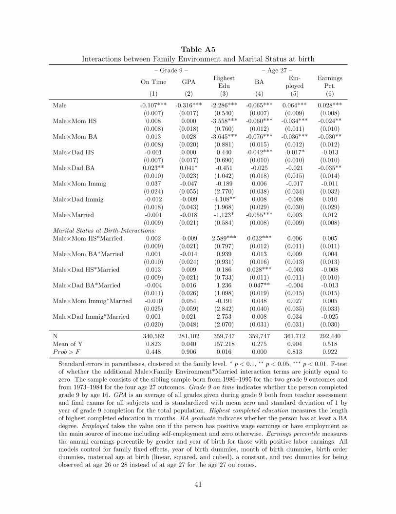
Table A5Interactions between Family Environment and Marital Status at birth

– Grade 9 – – Age 27 –

On Time GPAHighest

EduBA

Em-ployed

EarningsPct.

(1) (2) (3) (4) (5) (6)

Male -0.107*** -0.316*** -2.286*** -0.065*** 0.064*** 0.028***(0.007) (0.017) (0.540) (0.007) (0.009) (0.008)

Male×Mom HS 0.008 0.000 -3.558*** -0.060*** -0.034*** -0.024**(0.008) (0.018) (0.760) (0.012) (0.011) (0.010)

Male×Mom BA 0.013 0.028 -3.645*** -0.076*** -0.036*** -0.030**(0.008) (0.020) (0.881) (0.015) (0.012) (0.012)

Male×Dad HS -0.001 0.000 0.440 -0.042*** -0.017* -0.013(0.007) (0.017) (0.690) (0.010) (0.010) (0.010)

Male×Dad BA 0.023** 0.041* -0.451 -0.025 -0.021 -0.035**(0.010) (0.023) (1.042) (0.018) (0.015) (0.014)

Male×Mom Immig 0.037 -0.047 -0.189 0.006 -0.017 -0.011(0.024) (0.055) (2.770) (0.038) (0.034) (0.032)

Male×Dad Immig -0.012 -0.009 -4.108** 0.008 -0.008 0.010(0.018) (0.043) (1.968) (0.029) (0.030) (0.029)

Male×Married -0.001 -0.018 -1.123* -0.055*** 0.003 0.012(0.009) (0.021) (0.584) (0.008) (0.009) (0.008)

Marital Status at Birth-Interactions:Male×Mom HS*Married 0.002 -0.009 2.589*** 0.032*** 0.006 0.005

(0.009) (0.021) (0.797) (0.012) (0.011) (0.011)Male×Mom BA*Married 0.001 -0.014 0.939 0.013 0.009 0.004

(0.010) (0.024) (0.931) (0.016) (0.013) (0.013)Male×Dad HS*Married 0.013 0.009 0.186 0.028*** -0.003 -0.008

(0.009) (0.021) (0.733) (0.011) (0.011) (0.010)Male×Dad BA*Married -0.004 0.016 1.236 0.047** -0.004 -0.013

(0.011) (0.026) (1.098) (0.019) (0.015) (0.015)Male×Mom Immig*Married -0.010 0.054 -0.191 0.048 0.027 0.005

(0.025) (0.059) (2.842) (0.040) (0.035) (0.033)Male×Dad Immig*Married 0.001 0.021 2.753 0.008 0.034 -0.025

(0.020) (0.048) (2.070) (0.031) (0.031) (0.030)

N 340,562 281,102 359,747 359,747 361,712 292,440Mean of Y 0.823 0.040 157.218 0.275 0.904 0.518Prob > F 0.448 0.906 0.016 0.000 0.813 0.922

Standard errors in parentheses, clustered at the family level. ∗ p < 0.1, ∗∗ p < 0.05, ∗∗∗ p < 0.01. F-testof whether the additional Male×Family Environment*Married interaction terms are jointly equal tozero. The sample consists of the sibling sample born from 1986–1995 for the two grade 9 outcomes andfrom 1973–1984 for the four age 27 outcomes. Grade 9 on time indicates whether the person completedgrade 9 by age 16. GPA is an average of all grades given during grade 9 both from teacher assessmentand final exams for all subjects and is standardized with mean zero and standard deviation of 1 byyear of grade 9 completion for the total population. Highest completed education measures the lengthof highest completed education in months. BA graduate indicates whether the person has at least a BAdegree. Employed takes the value one if the person has positive wage earnings or have employment asthe main source of income including self-employment and zero otherwise. Earnings percentile measuresthe annual earnings percentile by gender and year of birth for those with positive labor earnings. Allmodels control for family fixed effects, year of birth dummies, month of birth dummies, birth orderdummies, maternal age at birth (linear, squared, and cubed), a constant, and two dummies for beingobserved at age 26 or 28 instead of at age 27 for the age 27 outcomes.

41

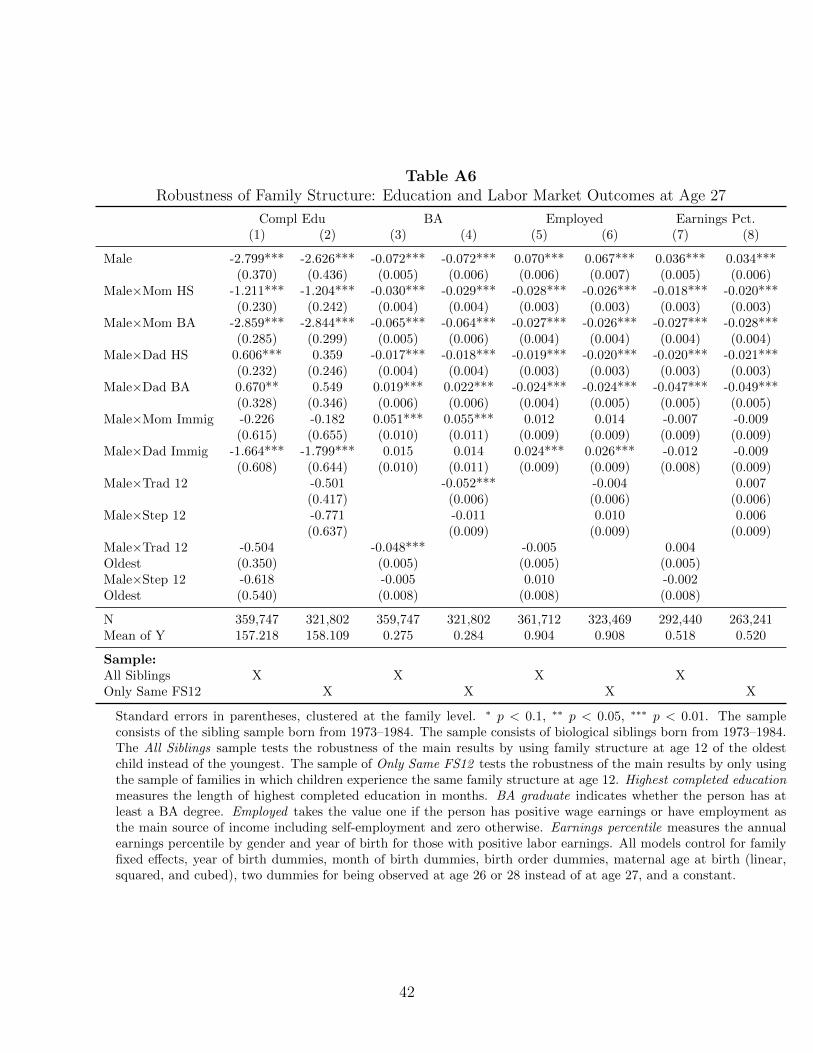
Table A6Robustness of Family Structure: Education and Labor Market Outcomes at Age 27

Compl Edu BA Employed Earnings Pct.(1) (2) (3) (4) (5) (6) (7) (8)

Male -2.799*** -2.626*** -0.072*** -0.072*** 0.070*** 0.067*** 0.036*** 0.034***(0.370) (0.436) (0.005) (0.006) (0.006) (0.007) (0.005) (0.006)

Male×Mom HS -1.211*** -1.204*** -0.030*** -0.029*** -0.028*** -0.026*** -0.018*** -0.020***(0.230) (0.242) (0.004) (0.004) (0.003) (0.003) (0.003) (0.003)

Male×Mom BA -2.859*** -2.844*** -0.065*** -0.064*** -0.027*** -0.026*** -0.027*** -0.028***(0.285) (0.299) (0.005) (0.006) (0.004) (0.004) (0.004) (0.004)

Male×Dad HS 0.606*** 0.359 -0.017*** -0.018*** -0.019*** -0.020*** -0.020*** -0.021***(0.232) (0.246) (0.004) (0.004) (0.003) (0.003) (0.003) (0.003)

Male×Dad BA 0.670** 0.549 0.019*** 0.022*** -0.024*** -0.024*** -0.047*** -0.049***(0.328) (0.346) (0.006) (0.006) (0.004) (0.005) (0.005) (0.005)

Male×Mom Immig -0.226 -0.182 0.051*** 0.055*** 0.012 0.014 -0.007 -0.009(0.615) (0.655) (0.010) (0.011) (0.009) (0.009) (0.009) (0.009)

Male×Dad Immig -1.664*** -1.799*** 0.015 0.014 0.024*** 0.026*** -0.012 -0.009(0.608) (0.644) (0.010) (0.011) (0.009) (0.009) (0.008) (0.009)

Male×Trad 12 -0.501 -0.052*** -0.004 0.007(0.417) (0.006) (0.006) (0.006)

Male×Step 12 -0.771 -0.011 0.010 0.006(0.637) (0.009) (0.009) (0.009)

Male×Trad 12 -0.504 -0.048*** -0.005 0.004Oldest (0.350) (0.005) (0.005) (0.005)Male×Step 12 -0.618 -0.005 0.010 -0.002Oldest (0.540) (0.008) (0.008) (0.008)

N 359,747 321,802 359,747 321,802 361,712 323,469 292,440 263,241Mean of Y 157.218 158.109 0.275 0.284 0.904 0.908 0.518 0.520

Sample:All Siblings X X X XOnly Same FS12 X X X X

Standard errors in parentheses, clustered at the family level. ∗ p < 0.1, ∗∗ p < 0.05, ∗∗∗ p < 0.01. The sampleconsists of the sibling sample born from 1973–1984. The sample consists of biological siblings born from 1973–1984.The All Siblings sample tests the robustness of the main results by using family structure at age 12 of the oldestchild instead of the youngest. The sample of Only Same FS12 tests the robustness of the main results by only usingthe sample of families in which children experience the same family structure at age 12. Highest completed educationmeasures the length of highest completed education in months. BA graduate indicates whether the person has atleast a BA degree. Employed takes the value one if the person has positive wage earnings or have employment asthe main source of income including self-employment and zero otherwise. Earnings percentile measures the annualearnings percentile by gender and year of birth for those with positive labor earnings. All models control for familyfixed effects, year of birth dummies, month of birth dummies, birth order dummies, maternal age at birth (linear,squared, and cubed), two dummies for being observed at age 26 or 28 instead of at age 27, and a constant.

42

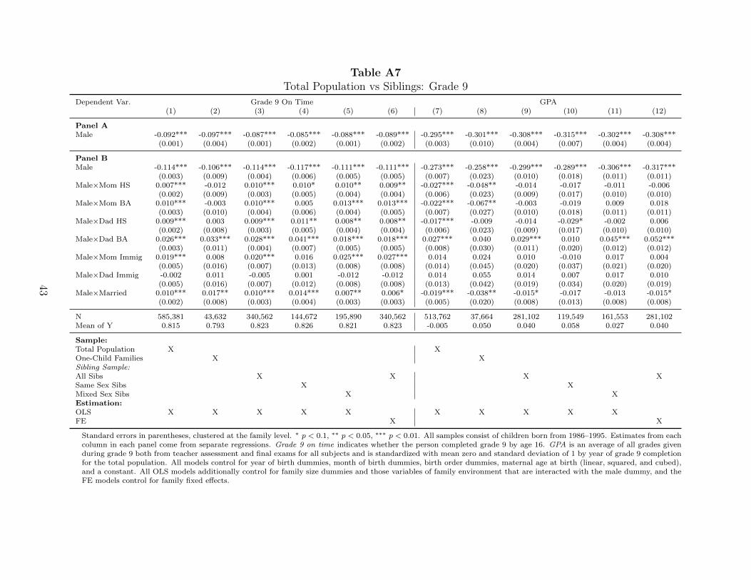
Table A7Total Population vs Siblings: Grade 9

Dependent Var. Grade 9 On Time GPA(1) (2) (3) (4) (5) (6) (7) (8) (9) (10) (11) (12)

Panel AMale -0.092*** -0.097*** -0.087*** -0.085*** -0.088*** -0.089*** -0.295*** -0.301*** -0.308*** -0.315*** -0.302*** -0.308***

(0.001) (0.004) (0.001) (0.002) (0.001) (0.002) (0.003) (0.010) (0.004) (0.007) (0.004) (0.004)

Panel BMale -0.114*** -0.106*** -0.114*** -0.117*** -0.111*** -0.111*** -0.273*** -0.258*** -0.299*** -0.289*** -0.306*** -0.317***

(0.003) (0.009) (0.004) (0.006) (0.005) (0.005) (0.007) (0.023) (0.010) (0.018) (0.011) (0.011)Male×Mom HS 0.007*** -0.012 0.010*** 0.010* 0.010** 0.009** -0.027*** -0.048** -0.014 -0.017 -0.011 -0.006

(0.002) (0.009) (0.003) (0.005) (0.004) (0.004) (0.006) (0.023) (0.009) (0.017) (0.010) (0.010)Male×Mom BA 0.010*** -0.003 0.010*** 0.005 0.013*** 0.013*** -0.022*** -0.067** -0.003 -0.019 0.009 0.018

(0.003) (0.010) (0.004) (0.006) (0.004) (0.005) (0.007) (0.027) (0.010) (0.018) (0.011) (0.011)Male×Dad HS 0.009*** 0.003 0.009*** 0.011** 0.008** 0.008** -0.017*** -0.009 -0.014 -0.029* -0.002 0.006

(0.002) (0.008) (0.003) (0.005) (0.004) (0.004) (0.006) (0.023) (0.009) (0.017) (0.010) (0.010)Male×Dad BA 0.026*** 0.033*** 0.028*** 0.041*** 0.018*** 0.018*** 0.027*** 0.040 0.029*** 0.010 0.045*** 0.052***

(0.003) (0.011) (0.004) (0.007) (0.005) (0.005) (0.008) (0.030) (0.011) (0.020) (0.012) (0.012)Male×Mom Immig 0.019*** 0.008 0.020*** 0.016 0.025*** 0.027*** 0.014 0.024 0.010 -0.010 0.017 0.004

(0.005) (0.016) (0.007) (0.013) (0.008) (0.008) (0.014) (0.045) (0.020) (0.037) (0.021) (0.020)Male×Dad Immig -0.002 0.011 -0.005 0.001 -0.012 -0.012 0.014 0.055 0.014 0.007 0.017 0.010

(0.005) (0.016) (0.007) (0.012) (0.008) (0.008) (0.013) (0.042) (0.019) (0.034) (0.020) (0.019)Male×Married 0.010*** 0.017** 0.010*** 0.014*** 0.007** 0.006* -0.019*** -0.038** -0.015* -0.017 -0.013 -0.015*

(0.002) (0.008) (0.003) (0.004) (0.003) (0.003) (0.005) (0.020) (0.008) (0.013) (0.008) (0.008)

N 585,381 43,632 340,562 144,672 195,890 340,562 513,762 37,664 281,102 119,549 161,553 281,102Mean of Y 0.815 0.793 0.823 0.826 0.821 0.823 -0.005 0.050 0.040 0.058 0.027 0.040

Sample:Total Population X XOne-Child Families X XSibling Sample:All Sibs X X X XSame Sex Sibs X XMixed Sex Sibs X XEstimation:OLS X X X X X X X X X XFE X X

Standard errors in parentheses, clustered at the family level. ∗ p < 0.1, ∗∗ p < 0.05, ∗∗∗ p < 0.01. All samples consist of children born from 1986–1995. Estimates from eachcolumn in each panel come from separate regressions. Grade 9 on time indicates whether the person completed grade 9 by age 16. GPA is an average of all grades givenduring grade 9 both from teacher assessment and final exams for all subjects and is standardized with mean zero and standard deviation of 1 by year of grade 9 completionfor the total population. All models control for year of birth dummies, month of birth dummies, birth order dummies, maternal age at birth (linear, squared, and cubed),and a constant. All OLS models additionally control for family size dummies and those variables of family environment that are interacted with the male dummy, and theFE models control for family fixed effects.

43

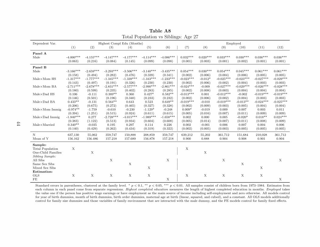
Table A8Total Population vs Siblings: Age 27

Dependent Var. Highest Compl Edu (Months) Employed(1) (2) (3) (4) (5) (6) (7) (8) (9) (10) (11) (12)

Panel AMale -4.000*** -4.155*** -4.147*** -4.177*** -4.114*** -4.086*** 0.032*** 0.020*** 0.033*** 0.030*** 0.036*** 0.036***

(0.063) (0.216) (0.084) (0.145) (0.099) (0.098) (0.001) (0.003) (0.001) (0.002) (0.001) (0.001)

Panel BMale -3.166*** -2.659*** -3.293*** -3.506*** -3.140*** -3.435*** 0.054*** 0.030*** 0.054*** 0.045*** 0.061*** 0.061***

(0.158) (0.494) (0.282) (0.476) (0.339) (0.341) (0.002) (0.006) (0.004) (0.006) (0.005) (0.005)Male×Mom HS -1.317*** -1.777*** -1.345*** -1.339*** -1.343*** -1.233*** -0.023*** -0.012* -0.025*** -0.023*** -0.027*** -0.029***

(0.143) (0.497) (0.191) (0.326) (0.230) (0.230) (0.002) (0.006) (0.002) (0.004) (0.003) (0.003)Male×Mom BA -2.711*** -2.678*** -2.831*** -2.577*** -2.990*** -2.861*** -0.024*** -0.009 -0.027*** -0.029*** -0.026*** -0.028***

(0.180) (0.599) (0.235) (0.402) (0.283) (0.285) (0.002) (0.008) (0.003) (0.004) (0.004) (0.004)Male×Dad HS 0.106 -0.111 0.389** 0.360 0.427* 0.582** -0.013*** 0.001 -0.012*** -0.002 -0.019*** -0.019***

(0.146) (0.501) (0.196) (0.340) (0.233) (0.232) (0.002) (0.006) (0.002) (0.004) (0.003) (0.003)Male×Dad BA 0.433** -0.131 0.564** 0.643 0.523 0.649** -0.019*** -0.010 -0.019*** -0.013** -0.024*** -0.025***

(0.206) (0.675) (0.272) (0.465) (0.327) (0.328) (0.002) (0.009) (0.003) (0.005) (0.004) (0.004)Male×Mom Immig -0.974** -1.759 -0.610 -0.230 -1.129* -0.248 0.009* -0.019 0.009 0.007 0.003 0.011

(0.394) (1.251) (0.515) (0.924) (0.611) (0.615) (0.005) (0.016) (0.007) (0.011) (0.009) (0.009)Male×Dad Immig -1.940*** 0.277 -2.728*** -4.015*** -1.989*** -1.658*** 0.002 0.000 0.005 -0.020* 0.018** 0.024***

(0.383) (1.122) (0.513) (0.934) (0.604) (0.608) (0.005) (0.014) (0.007) (0.011) (0.008) (0.009)Male×Married 0.340** -0.035 0.195 0.297 0.114 0.226 0.002 -0.001 0.006 0.007 0.004 0.006

(0.140) (0.429) (0.262) (0.434) (0.319) (0.322) (0.002) (0.005) (0.003) (0.005) (0.005) (0.005)

N 637,130 55,062 359,747 150,888 208,859 359,747 639,212 55,202 361,712 151,684 210,028 361,712Mean of Y 156.162 156.486 157.218 157.689 156.878 157.218 0.900 0.888 0.904 0.908 0.901 0.904

Sample:Total Population X XOne-Child Families X XSibling Sample:All Sibs X X X XSame Sex Sibs X XMixed Sex Sibs X XEstimation:OLS X X X X X X X X X XFE X X

Standard errors in parentheses, clustered at the family level. ∗ p < 0.1, ∗∗ p < 0.05, ∗∗∗ p < 0.01. All samples consist of children born from 1973–1984. Estimates fromeach column in each panel come from separate regressions. Highest completed education measures the length of highest completed education in months. Employed takesthe value one if the person has positive wage earnings or have employment as the main source of income including self-employment and zero otherwise. All models controlfor year of birth dummies, month of birth dummies, birth order dummies, maternal age at birth (linear, squared, and cubed), and a constant. All OLS models additionallycontrol for family size dummies and those variables of family environment that are interacted with the male dummy, and the FE models control for family fixed effects.

44