Embed Size (px)
Citation preview

Gender Gaps in Unemployment Rates in Argentina*
Ana Carolina Ortega Masagué**
March 2006
* I am grateful to Juan Francisco Jimeno, Daniel Kotzer, Raquel Carrasco and José María Labeaga for their helpful suggestions. I also thank Cristina Fernández, Emma García and Juan Ramón García for their comments. The usual disclaimer applies.
** Universidad de Alcalá de Henares and FEDEA.

Abstract The gender gap in unemployment rates in Argentina increased noticeably during
the nineties. The aim of this paper is to study the reasons why women, once they have
decided to participate in the labor market, have lower probabilities of being employed
than men. The results indicate that the larger women’s unemployment rate derives from
their lower probability of transition from unemployment to employment, which is
explained by differences in the effects of men’s and women’s characteristics.
JEL Code: J16, J64 Keywords: gender gap, unemployment rates.
1

1. Introduction
The literature that studies gender gaps in labor force participation rates and
wages, as well as the literature that analyzes occupational segregation by gender cover
differents countries and time periods and are by now very large.1 On the contrary, the
studies that examine gender gaps in unemployment rates are much more scarce. Lately,
however, there has been a growing concern about the factors that may contribute to
explain these gaps.
As seen in Table 1, developed countries such as Greece, Spain, Italy, France and
Portugal show important gender gaps in unemployment rates. Developing countries
have not kept apart from this phenomenon. Table 2 shows that in some Latin American
countries gender gaps in unemployment rates are even more important than in
developed countries.
The evolution of the gender gap in unemployment rates in Argentina, from the
beginning of the 1980s to the present days, has showed some notable peculiarities that
make the Argentinian labor market an interesting case of study. Figure 1 presents the
evolution of male and female unemployment rates in the Great Buenos Aires between
1980 and 2002. As can be seen in it, in the 1980s female unemployment rates were a
little bit higher than male unemployment rates (except in 1985). However, from 1992 to
2000, the differential between both rates increased noticeably. In particular, in 1996 the
gender gap in unemployment rates reached more than 5 percentage points. Later, it
decreased and in 2002 women’s unemployment rate was simitar to men’s.2
1 For an introduction to these topics see Altonji and Blank (1999). Some of the most recent articles that study gender wage gaps are Blau and Kahn (2004) for the United States, Beblo et. al (2003) for the European Union (EU) countries, Dolado and Llorens (2004) for Spain, Saavedra for some Latin American countries and Esquivel and Paz (2003) and Paz (2000) for Argentina. Among the papers that analyze occupational segregation by gender we stand out Petrongolo (2004) for the EU countries and Dolado et al. (2002) for the EU countries and the United States. All these topics are also analyzed in a study of the Organization for Economic Co-operation and Development (OECD, 2002) and in a paper of the Internacional Labor Organization (ILO, 2003) 2 The equality of men’s and women’s unemployment rates in 2002 can be basically explained by two reasons. Firstly, at the beginning of that year the government implemented the Household Head Plan, which main objective is providing economic help to unemployed household heads. In addition, the Household Head Plan seeks to achieve the labor reinsertion of its beneficiaries by means of training courses, productive work for the State and/or agreements with firms. Then, most of the beneficiaries of the plan are working. (For a more detailed description of the Household Head Plan, see López Zadicoff and Paz (2003)). Considering the individuals that receives benefits from the Household Head Plan as employed rose men’s unemployment rate above women’s. On the contrary, if the beneficiaries of the plan
2
In response to the above evidence, the aim of this paper is to study the factors
that determined the gender gaps in unemployment rates in Argentina during the 1995-
2001 period. In other words, we are interested in studying the reasons why women, once
they have decided they want a job, have lower probabilities of being employed than
men.
The economic theory suggests that there are lot of possible explanations for the
gender gaps in unemployment rates. On the demand side, discrimination has been
pointed out as one of the factors that would explain the higher female unemployment
rate. The economic models distinguish two main sources of discrimination. The first
one, formulated by Becker, refers to the prejuices that, at least, part of the employers
might have against women. The second one refers to the so called statistical
discrimination. It arises as a consequence that employers, in the presence of imperfect
information, assume that women, on average, have a lower level of labour market
attachment and are less qualified than men. On the supply side, the increase in the
female labor force participation combined with the existence of bottlenecks in the
economy’s capacity to absorb new labor force entrants, the lower attachment of women
to the labor force, reflected in higher movements into and out of the labor force and a
lower job search intensity, as well as their different characteristics have been some of
the factors mentioned as possible causes of the gender gaps in unemployment rates.
Political measures intended for eliminating women’s inferiority in the labor
market will depend on the causes of the gender gap in unemployment rates. These
measures will not only improve women’s relative position in the labor market, but also
will contribute to mitigate the serious problem of unemployment, increasing the
employment opportunities of an important part of the labour force.
were classified as unemployed, women’s unemployment rate would be approximately 6,6 percentage points higher than men’s. Given the lower women’s labor force participation rate, it is probable that a high percentage of those that were inactive before the plan’s implementation entered the labor force to receive its benefits. Secondly, the sudden reduction in the level of activity and the collapse of the Convertibility Plan at the end of 2001 affected the degree of stability of employment of different sectors in different ways. In particular, the manufacturing sector, in which men constitute a relatively large proportion of total employment, experienced higher employment destruction rates than the service sector, dominated by women.
3

The rest of the paper is structured as follows. In section 2 we review the existing
literature on gender gaps in unemployment rates. In section 3 we present some
indicators of women’s situation in the argentinian labor market during the last two
decades. In section 4 we study the determinants of the unemployment probability. As
we will see in more detail, gender plays an important rol, with women having a higher
unemployment probability than men. This difference seems to be explained not by
differences in the characteristics of men and women but by differences in the market
returns to these characteristics for both groups. In section 5 we examine the differences
in the flows between labor market states of men and women that contribute to determine
the gender gaps in unemployment rates. The larger women’s unemployment rate is the
result of their larger probability of moving from employment to inactivity and their
lower probability of moving from unemployment to employment. However, results
suggest that, for some reason, flows involving inactivity are similar to direct flows
between employment and unemployment. Therefore, in section 6 we focus on studying
the differences in the flows from employment to unemployment and from
unemployment to employment between men and women. On the one hand, women’s
probablity of moving from employment to unemployment is lower than men’s. An
important part of this difference is explained by differences in the characteristics of both
groups. On the other hand, the probability of transition from unemployment to
employment is higher among men than among women. Such difference is explained
almost exclusively by differences in the effects of men’s and women’s characteristics.
Finally, section 7 concludes.
2. Literature Review
The economic literature has devoted little efforts to the study of gender gaps in
unemployments rates. From 1950 to 1980, women’s unemployment rate was higher
than men’s in the United States. In order to study this phenomenon, Johnson (1983)
redefines the female unemployment rate considering domestic production as an
employment. Using data from the Current Population Survey (CPS), she obtains that
women’s unemployment rate so defined is lower than men’s. In addition, she finds that
the gender gap in unemployment rates varies procyclically, which is not the expected
result if the gender gap in unemployment rates is due to differences in the productive
opportunities of men and women. Finally, she presents evidence that a woman has a
4

lower unemployment probability than a man with equal characteristics. Thus, she
concludes that an important part of the observed differential could be attributed to the
definition and methodology used to calculate unemployment rates rather than to
discrimination of employers against women.
However, in the 1980s the difference between male and female unemployment
rates in the United States virtually disappeared. Then, the economic literature focuses on
analizing the possible causes of the equality of both rates. DeBoer and Seeborg (1989)
study the changes in the probabilities of transition between different labor market states.
Using data from the Bureau of Labor Statistics (BLS), the authors find that about half of
the narrowing of the unemployment rate differential during the 1968-1985 period was
due to the increasing labor force attachment of women and the decreasing attachment of
men. The other half reflects changes in men’s and women’s tendencies to move between
employment and unemployment, attributed primarily to the decline of male-dominated
industries. Using data from the CPS, Mohanty (1998) obtains that the disappearance of
the gap between male and female unemployment rates results partly from a considerable
decline in hiring discrimination against females during the last two decades. This study
also finds that the growth of employment in government and in the service sector, and
migration of workers from the South to other regions have contributed significantly to
the convergence of male and female unemployment rates. More recently, using the same
database, Mohanty (2003) establishes that the ability of employers to pay lower wages
to women raises average female employment probabilities which, in turn, yields lower
female unemploymet rates. Then, wage discrimination, among other factors, would be
explaining the equality between male and female unemploymet rates. Therefore, the
equality of male and female unemploymet rates should not be confused with absence of
discrimination against women.
Using macro data for the Canadian economy, Myatt and Murrell (1990) find that
bottlenecks in the economy’s ability to absorb new labor force entrants do not explain
the gap between male and female unemployment rates. According to these authors,
the most important determinant of the differential between male and female
unemployment rates is the level of the minimum wage. The lower attachment of
women to the labor force explains only one-quarter of this differential.
5

In the OECD framework, using data from the ECHP, Azmat, Güell and Manning
(2004) show that in countries where there is a large gender gap in unemployment
rates, particularly the Mediterranean countries, there is a gender gap in both flows
from employment to unemployment and from unemployment to employment. They
investigate different hypotheses about the sources of these gaps. Most hypotheses find
little support in the data. However, the gender gap in unemployment rates does seem
to correlate with attitudes on whether men are more deserving of work than women.
Thus, discrimination against women may explain part of the gender gap in
unemployment rates in the Mediterranean countries.
Using data from the European Community Household Panel (ECHP) for the
1994-1998 period, Eusamio (2004) studies the causes of the large differential that
exists between male and female unemployment rates in Spain, extending the analysis
to the Portugal’s case. When studying the empirical determinants of the hazard rates
from employment and unemployment of men and women, she finds that women have
more difficulties to leave unemployment and a higher probability of leaving
employment, at least during the first year in each state. Finally, using a non-linear
Oaxaca decomposition, she obtains evidence that men and women have similar
characteristics that, nonetheless, are rewarded differently.
Regarding less developed countries, Ham, Svejnar and Terrell (1999) investigate
the reasons why women’s unemployment rate is above men’s in the Czech and Slovak
Republics. They find that the differences between men’s and women’s probabilities of
leaving unemployment are explained more by differences in returns to characteristics
than by differences in observed characteristics. Therefore, they conclude that
differences in men’s and women’s behaviour and the practices of employers and
institutions towards gender are dominating the differences between men’s and
women’s exit rates from unemployment in both countries. Finally, Lauerová and
Terrell (2002) analyze the determinants of the gender differences in unemployment
rates in post-communist economies, specially the Czech Republic. When analysing
the flows between labor market states, they find that an important part of the gender
gap in unemployment rates results from married women’s lower probability of
moving from unemployment to employment and from single women’s lower
probability of moving from inactivity to employment.
6
3. Women’s Situation in the Argentinian Labor Market
Argentinian legislation, as the one of most democratic western countries,
recognizes the fundamental principle of equity between men and women at work. The
National Constitution establishes equity of all inhabitants in the admission to
employment, without any other condition but suitability, and equal remuneration for
equal job. Moreover, international relevant norms in the field of gender discrimination,
such as the United Nations’ Convention for the Elimination of All Forms of
Discrimination against Women and the ILO’s agreements related to women’s
employment, are supported by Argentina. At the national level, the employment
relationships in the private sector are regulated by the Work Contract Law (Ley de
Contrato de Trabajo Nº 20744), while public sector workers are protected by the
National Public Employment Regulation Law (Ley Marco de Regulación del Empleo
Público Nacional Nº 25164). These laws clearly express the need to defend equity
between men and women workers. Finally, this general legislation is complemented by
other numerous detailed regulations.3
During the last two decades, women’s situation in the Argentinian labor market
has been characterized by two important facts: (i) women’s unemployment was larger
than men’s, and (ii) female labor force participation increased noticeably.
Figures 2 to 5 present male and female unemployment rates in the Great Buenos
Aires from 1980 to 2002 for groups between 15 and 19 years, 20 and 34 years, 35 and
49 years and 50 and 64 years, respectively. For the first three age groups, the gender
gaps in unemployment rates were small in the 1980s and widened considerably in the
1990s. Those under 19 years present the largest gender gaps in unemployment rates. On
the contrary, the gender gaps in unemployment rates for those over 50 years were, in
general, very small and, sometimes, even favorable to women.
Figures 6 to 10 present male and female labor force participation rates in the
Great Buenos Aires from 1980 to 2002 for the population between 15 and 64 years, as
3 Based on this legislation, in December 2002 a judicial sentence, without precedents in the country, condemned Freddo ice-cream shop to employ women exclusively for considering it discriminated them. The sentence was based in the fundamental fact that, in December 1999, the firm had 646 men and 35 women workers.
7

well as for the age groups mentioned above. As can be seen in the first of them,
following a world trend, female labor force participation rates have risen noticeably
during the last two decades. From 1983 to 2002, female participation rate in the Great
Buenos Aires has increased from 23% to 37%. In particular, its increase was more
intense during the 1990s, which may be explained, among others, by the following two
factors: (i) the notable decrease of the fertility rate, that falled from around 3,1 children
per women in the 1980s to 2,7 children per women in the 1990s; and (ii) the so called
added worker effect, by which some women, in view of the unemployment situation of
their husbands, decided to participe actively in the labor market.4 The participation rates
of women between 20 and 34 years, 35 and 49 years and 50 and 64 years have shown a
similar behaviour. In particular, the participation rate of the cohort between 50 and 64
years has shown the most pronounced growth. On the contrary, the participation rate of
those under 19 years has showed a decreasing trend. This is due to the higher levels of
education of the younger cohorts that, as a consequence, delay their entrance to the
labour market. Their participation rate was lower than that of the other cohorts (except
for the first years of the 1980s when the participation rate of women over 50 was
lower).
4. Unemployment Probability
4.1 Probit Models
The economic literature points out the importance of taking into account the
different characteristics of men and women when comparing their labor market
outcomes. In other words, it is probable that, al least, part of the gender gap in
unemployment rates is explained by differences in the characteristics of both groups. In
order to investigate this hypothesis, we use a discrete choice model.
Let yi be the dependent variable that takes value one if the individual is
unemployed and zero if she is employed. We model the unemployment probability
conditional to a group of exogenous variables, xi, obtaining
( ) ( )| Pr 1| ( ´i i i i iE y x y x F xβ= = = )
4 For an analysis of the added worker effect among married women in Argentina, see Díaz-Bonilla (2004).
8

where β represents a group of parameters and ( )F ⋅ is a cumulated density function. For
an N individuals random sample, the likelihood function of this model is written as
1
1
( ) (1 ( ))i i
Ny y
i ii
L F x F xβ β −
=
= −∏
In the empirical implementation F is specified as a normal distribution 2(0, )uN σ ,
resulting in a probit model of the form
´
Pr( 1) ( ) ( ´ )ix
i iy t dtβ
φ β−∞
= = = Φ∫ x
which is estimated by maximum likelihood.
4.2 Decomposition of the gap in unemployment probability
The decomposition presented in this section consists in an extension of the well-
known Oaxaca’s (1973) and Blinder’s (1973) decomposition.5 Let xM and xF be the
characteristics of men and women, respectively and let βM and βF be the returns to these
characteristics. The gender gap in the average unemployment probability can be
decomposed in the following way
´ ´ ´ ´ ´ ´( ) ( ) ( ) ( ) ( ) (F F M M F F F M F M M Mx x x x xβ β β β β β⎡ ⎤ ⎡Φ −Φ = Φ −Φ + Φ −Φ⎣ ⎦ ⎣ )x ⎤⎦
or alternatively,
´ ´ ´ ´ ´ ´( ) ( ) ( ) ( ) ( ) (F F M M M F M M F F M F )x x x x xβ β β β β β⎡ ⎤ ⎡Φ −Φ = Φ −Φ + Φ −Φ⎣ ⎦ ⎣ x ⎤⎦
where Φ represents the average unemployment probability. In the first (second)
equality it is assumed that βF (βM) is the vector of coefficients that would prevail in
absence of discrimination. The first term on the right-hand side of the above equalities
5 For a detailed description of the gender wage gaps decomposition methods, see Beblo et al. (2003).
9

measures the difference in the average unemployment probability that is explained by
differences in the observed characteristics, whereas the second term gathers the
differences due to different returns to those characteristics. This second term is
associated with the discriminatory component of the gap. However, as not all the
characteristics that affect the unemployment probability can be taken into account,
because information about them is not available or because they are unobservable, this
term it is not an accurate measure of discrimination and its magnitude will be
overestimated. Nonetheless, when it represents a large percentage of the total gap, the
possibility that discrimination exists cannot be ruled out.6
The general methodology proposed by Yun (2004) allows us to obtain the
individual contribution of each variable when applying the Oaxaca-Blinder
decomposition to a non-linear function. Then, the detailed decomposition of the above
equalities can be written as
´ ´ ´ ´ ´ ´
1 1( ) ( ) ( ) ( ) ( ) (
i i
K KF F M M F F F M F M M M
xi i
x x W x x W xββ β β β β β∆ ∆= =
⎡ ⎤ ⎡Φ −Φ = Φ −Φ + Φ −Φ⎣ ⎦ ⎣∑ ∑ )x ⎤⎦
where
( )( )i
F M Fi i
x F M F
x xWx x
ββ
∆−
=−
, (( )i
M F Mi i iM F M
xWx
β)β β
β β∆
−=
− y
1 1
1i i
K K
xi i
W W β∆ ∆= =
= =∑ ∑
or alternatively,
´ ´ ´ ´ ´ ´
1 1( ) ( ) ( ) ( ) ( ) (
i i
K KF F M M M F M M F F M F
xi i
x x W x x W x xββ β β β β β∆ ∆= =
⎡ ⎤ ⎡Φ −Φ = Φ −Φ + Φ −Φ⎣ ⎦ ⎣∑ ∑ )⎤⎦
where
( )( )i
F M Mi i i
x F M M
x xWx x
ββ
∆−
=−
, (( )i
F F Mi i iF F M
xWx
β)β β
β β∆
−=
− y
1 1
1i i
K K
xi i
W W β∆ ∆= =
= =∑ ∑
6 Neumark (1988) assumes that the vector of coefficients that would prevail in absence of discrimination is the one that results from combining men and women in a single estimation. In this case, the gender gap in the average unemployment probability is decomposed in three parts. The first term, as before, measures the difference in productivity of both groups. The second term, estimates the discrimination in favor of one of the groups, whereas the third term gathers the discrimination against the other group.
10

where K is the number of explanatory variables and , M Fx x are the average
characteristics of men and women, respectively.
4.3 The data
To investigate the hypothesis that differences in the characteristics of men and
women can explain the gap in their unemployment rates we use data drawn from the
Permanent Household Survey (Encuesta Permanente de Hogares). This survey is carried
out by the National Institute of Statistics and Censuses twice a year (in May and
October) since 1974.7
The sample used comprises 28 Argentinean cities from May 1995 to October
2001.8 Given the evidence presented above, only the individuals between 15 and 54
years were included in the sample. The sample contains a total of 357.662 observations,
including salaried workers and unemployed workers that search actively for a job and
for which there is no missing information.
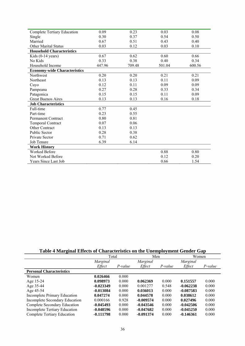
Table 3 presents some descriptive statistics of employed and unemployed men
and women. Regarding individual characteristics, unemployed women tend to be
younger than unemployed men, whereas employed men tend to be younger than
employed women. A higher proportion of women are divorced, separated or widow,
whereas a larger percentage of men are married. A higher (lower) proportion of
employed (unemployed) women are single. In addition, women have higher education
levels than men in the same labor market state. Regarding household characteristics, in
percentage terms, there are more unemployed women than men that have children under
14 years, whereas there are fewer employed women than men that have children under
14. The geographical distribution of men and women is very similar. Finally, women’s
household income is higher than men’s.
7 In 1998 and 1999 a third survey was carried out in August. 8 Up to May 1995 the survey comprised 25 cities. In October 1995 three more cities were incorporated into the survey.
11

4.4 The gender gap
The explanatory variables included in the model comprise individual
characteristics (gender, age, education, marital status), family characteristics (presence
of children at home, rest of the family income) and economy-wide characteristics
(region, year). All variables are dummies, except the income that is continuous.9 Given
the inexistence of a general unemployment protection system in Argentina, it is
interesting to study the influence of the rest of the family income on the unemployment
probability. In absence of unemployment subsidies, the rest of the family income
becomes the only source of income of the unemployed individuals. In this case, income
may have two opposite signed effects on the unemployment probability. On the one
hand, a higher family income rises the reservation wage of the individual, which implies
a larger probability of rejecting a job offer. On the other hand, a larger family income
improves the job search conditions, which favors the arrival of job offers. Specifying
the relationship between the unemployment probability and the rest of the family
income as a cuadratic function allows us to capture the net effect for the different levels
of income.10
When only the gender dummy is included in the model, its marginal effect is
equal to 0.009674, being significant at a one percent level.11 This marginal effect is
comparable to the gender gap in the aggregate unemployment rates. When the rest of
the variables are included in the model (first and second columns of Table 4) the
marginal effect of the gender variable increases noticeably.12 Therefore, the individual
characteristics do not contribute to explain the gender gap in unemployment rates.
Columns 3-6 of Table 4 present the results of estimating separate regressions for
men and women. As pointed out above, from these estimations it is possible to
decompose the differencial between the average unemployment probability of men and
women into two parts. Table 5 presents the results of such decomposition. The sign of
9 For a more detailed description of the variables definition, see Appendix C. 10 For more details, see Arranz et al. 11 In the case of a probit model, the coefficients cannot be interpreted as the partial derivative of the unemployment probability with respect to the independent variables. Then, in this section we present, instead, the marginal effects. 12 The results are very similar if, instead of using region and year dummy variables to measure the state of the business cycle, we used regional unemployment rates.
12

the first term is negative which implies that women have larger productive
characteristics than men. The second term is positive which means that the market
returns to men’s characteristics are larger than the returns to women’s characteristics.
Moreover, given that women are more productive than men, this second component is
higher than the observed differential between the average unemployment probabilities.
Thus, its magnitude results very high, varying between 173% and 343% of the observed
differential.13 Considering βF as the coefficient that would prevail in absence of
discrimination leads to a larger differential due to differencies in the treatment of men
and women and to a smaller differential explained by different characteristics of both
groups than when using βM.14
The detailed decomposition shows that an important part of the difference
between men’s and women’s average unemployment probabilities is explained by
differences in the returns associated with marital status. 15
4.5 Other variables
In this section we briefly analyze the influence of the rest of the explanatory
variables included in the model on the unemployment probability. In the case of men,
the relationship between unemployment probability and age has a U shape, reaching a
minimum for the 25-34 years group. In the case of women, unemployment probability
decreases with age. In both cases, unemployment probability is higher among young
people. Educational level has a negative influence on the unemployment probability.
Single, divorced or widow individuals, as well as those that have children under 14
years, have higher possibilities of being unemployed. When considering all individuals,
the relationship between unemployment probability and family income is not lineal, 13 The results obtained when using Neumark’s decomposition are between those obtained when considering βF and βM as the returns that would prevail in absence of discrimination. 14 Oaxaca and Ramson (1984) also find this difference when using βF and βM. 15 It is probable that unobserved characteristics are also important when explaining the differences between men’s and women’s unemployment probabilities. As we have panel data, one possibility in the framework of the fixed effects approach that would allow us to take into account unobserved heterogenity is to estimate a conditional logit model. However, for doing this it is necessary that the explanatory variables have enough time variation and the key variable here is time invariant. Also, it would be possible to use a random effects approach. The problem is that the assumptions required to apply this method are very restrictive. In any case, as Azmat et al. (2004) suggest, it is probable that unobserved characteristics related to labor force participation widen the differential between men’s and women’s unemployment probabilities rather than contributing to explain it.
13

with an inverted U shape.16 Unemployment probability is higher during recession years
and in the more important regions of the country where a significant fraction of the
labor force is concentrated.
In sum, in this section we have showed that the gender gaps in unemployment
rates cannot be explained by differences in the characteristics of men and women. In the
next section we analyze if the gender gap in unemployment rates is the result of
differences in the flows between labor market states.
5. Flows between Labor Market States: Transition Probabilities
Considering three labor market states (employment, e, unemployment, u, and
inactivity, i), the transition probability from state k to state j (hkj) is defined as:
kjkj
k
Flowh
Stock= , ,k j e u i,=
where is the number of individuals that at time t were in state k and in time t+∆
are in state j, and is the number of individuals that at time t were in state k.
kjFlow
kStock
If the labor market is in a steady state, then the unemployment rate (UR) can be
expressed as a function of transition probabilities between the three labor market states17
/(1 )( / ) ( / )
eu eu ui
eu hue ei ui ie iu
h h hURh h h h
α α+
= − ++ h
where
( ) (ie ui iu ei
ie ui eu ue iu ei eu ue
h h h hh h h h h h h h
α)
+=
+ + + + +
)
16 The turning point or minimum of this curve is around 263 Argentinian pesos. 17 The labor market is in a steady state when the flows into and out of employment are equal ( ), as are the flows into and out of unemployment
( ).
(ue ie eu eih U h I h h E+ = +
( )eu iu ue uih E h I h h U+ = +
14
According to this equation, the overall unemployment rate can be interpreted as
a weighted average of two unemployment rates. The first term on the right-hand side is
the unemployment rate that would prevail if there were no flows into and out of
inactivity. The second term on the right-hand side is the unemployment rate that would
prevail if there were no directs flows between employment and unemployment and there
were only indirect flows through inactivity. The weight α is a measure of the relative
importance of flows via inactivity in generating unemployment.
The above equation implies that increases in , and lead to decreases in
the unemployment rate, while increases in , and lead to increases in the
unemployment rate. Therefore, the gender gaps in unemployment rates are due to
differences in these probabilities.
ueh uih ieh
euh eih iuh
Table 6 presents the average transition probabilities between labor market states
for the considered period (1995-2001). From these probabilities, we calculate the
different components of the above equation for men and women. The probabilities are
multiplied by 100 so that they can be interpreted as the percentage of individuals that
moves from one labor market state to another. The data used result from matching those
individuals that are present in the sample in two consecutive waves. Each semester one
quarter of the households is renewed, enabling us to follow individuals for a period of
up to four consecutive semesters. As the interval between two observations are six
months, multiple transitions can take place between them. However, we assume that if a
transition has taken place this is unique.
Since the Argentinian economy has faced enormous structural changes within
the last years, it is difficult to argue that its labor market is in a steady state.
Nevertheless, as seen in the last two rows of the table, male and female unemployment
rates calculated according to the above equation are quite similar to unemployment rates
calculated using the convential formula U/(U+E).
The higher women’s unemployment rate is the result of their larger probability
of moving from employment to inactivity (11.91% vs. 3.35%) and their lower
15

probability of moving from unemployment to employment (27.50% vs. 49.17%)18
which, in turn, leads to a longer average duration of their unemployment spells. 19
As the weight α is small and the two components of the unemployment rate are
similar, the labor market state of inactivity does not seem to be relevant when
determining men’s unemployment rate. In the case of women, the weight α is higher.
However, as the two components of the unemployment rate are quite similar, ignoring
the labor market state of inactivity will not lead to seriously misleading conclusions.
The results do not suggest that flows involving inactivity are not important to explain
the gender gaps in unemploymet rates, but, for some reason, they are similar to direct
flows between employment and unemployment. Then, in the following sections the
interest will focus on flows between employment and unemployment, ignoring flows
involving inactivity.20
6. Flows between Employment and Unemployment
6.1 Duration Models21
Suppose an individual i enters a labor market state at time t=0. The probability
that this person leaves that state at time t>0 is given by a proportional hazard model of
the form
( , ) ( ) exp( ´ )i it x t xθ λ β=
where xi is a vector of time-invariant explanatory variables, ( )tλ is the baseline hazard
function and β is a vector of parameters to be estimated. The continuous survivor
function at time t is22
( )0 0
( , ) exp ( , ) exp ( )exp( ´ ) exp exp ´ ( )i i
t ti iduS t x u x u x du x u duθ λ β β⎡ ⎤ ⎡ ⎤ ⎡
⎢ ⎥ ⎢ ⎥ ⎢⎣ ⎦ ⎣ ⎦ ⎣= − = − = −∫ ∫ ∫0
tλ ⎤
⎥⎦
18 The results are similar to those obtain by Pessino and Andrés (2000). 19 In October 2001, the percentage of unemployed women that has been in this situation for more than 6 (12) months was 39.29% (11.3%) versus 23.37% (6.3%) of men. 20 Also, we do not have enough statistic information to analyze the labor market state of inactivity. 21 Some of the papers that use duration models to analyze flows between labor market states in Argentina are Arranz et al. (2000), Beccaria and Mauricio (2003), Cerimedo (2004), Galiani and Hopenhayn (2001), Hopenhayn (2001) and Pessino and Andrés (2003)
22 By definition ln ( , )
( , ) ii
d S t xt x
dtθ
−= .
16

Although durations are continuous, they are observed at discrete time intervals.
To simplify, intervals are assumed to be of unit lenght. Given a discrete random
variable that represents the time at which the end of the spell of individual
i occurs, the survivor function at the start of the t
)1,i i iT t t∈ −⎡⎣
i-th interval is given by
{ }1 ( 1,i i i i )prob T t S t x≥ − = −
and the probability of exit in the ti-th interval is
){ }1, ( 1, ) ( , )i i i i i i iprob T t t S t x S t x∈ − = − −⎡⎣
Thus, the hazard of exit in the ti-th interval, defined as the probabilty of leaving a
state in the ti-th interval, given that it was not left until the ti-1-th interval, is
){ } ){ }{ }
1, ( , )( , ) 1, / 1 11 ( 1
i i i i ii i i i i i i
i i i i
prob T t t S t xh t x prob T t t T t, )prob T t S t x
∈ −⎡⎣= ∈ − ≥ − = = −⎡⎣ ≥ − −
Substituting the expression obtained
( )( ) exp exp, 1 ´ ( )i i ih t ix x tβ γ= − − +⎡ ⎤⎣ ⎦
where is constant within duration intervals and varies between
them. This feature of the baseline hazard function allows us to introduce duration
dependence, that is, that the probability of moving from one state to another depends on
the duration of the original state. In particular, we chose a non-parametric specification
for the baseline hazard function, based in a group of dummy variables that indicates the
duration of the original state.
1( ) log ( )i
i
t
i ttγ λ
−= ∫ u du
While some persons leave the state during an interval, others remain in the state.
The former group, that is not censured, is identified using a censoring indicator 1ic = .
17

For the latter group, whose observations are right-censored, . Given these
assumptions, the likelihood function can be written as
0ic =
[{ } { }{ }1
1, ) (1 )N
i i i i i ii
iL c prob T t t c prob T t=
= ∈ − + −∑ ≥
i
where N is the number of individuals. Taking logarithms and replacing above
expressions
[ ]{ }1
log log ( 1, ) ( , ) (1 ) log ( , )N
i i i i i i ii
L c S t x S t x c S t x=
= − − + −∑
This expression can be written in terms of the hazard function as
[ ] [ ]1
1 1 1
log log ( , ) 1 ( , ) (1 ) log 1 ( , )i it tN
i i i i i ii s s
L c h t x h s x c h s x−
= = =
⎧ ⎫⎧ ⎫ ⎧⎪ ⎪= − + − −⎨ ⎨ ⎬ ⎨⎪ ⎪⎩ ⎭ ⎩⎩ ⎭
∑ ∏ ∏⎫⎬⎬⎭
( )1 1 1
( , )log log log 1 ( , )1 ( , )
itN Ni i
i ii i si i
h t xL c h s xh t x= = =
⎡ ⎤= +⎢ ⎥−⎣ ⎦∑ ∑∑ −
Discrete time duration models can be regarded as a sequence of binary choice
equations defined on the survivor population at each duration.23 In this model, the exits
or stays at each period are considered as an observation. Let be an indicator variable
that takes value one if individual exits the state during the interval and zero
otherwise. Thus, for individuals that do not exit the state
ity
i )1,i it t−⎡⎣
0ity = in all periods, while for
individuals that exit the state 0ity = in all periods, except the one in which the exit
produces. Then, the logarithm of the likelihood function is written as
( ){ }1 1
log log ( , ) (1 ) log 1 ( , )itN
i i ii s
L y h s x y h s x= =
= + − −∑∑ i
In order to have access to longer spells and since we can only observe
individuals for a maximum of 4 semesters, we include in our sample individuals whose
23 See Jenkins (1995), Carrasco (2001) and Bover et al. (2002).
18

spells had already started before they were first interviewed. Therefore, we have to
condition exit rates on the probability of the spell surviving up to the time of the first
interview. For doing this, we use the retrospective information reported in it. Suppose
that at the time of the first interview the individual i has remained ji periods in the state
and remains in it for another ki periods. Then, total duration is i it j ki= + . The log-
likelihood function is rewritten as
( ) ( )1
1 1 1
log log 1 ( , ) log ( , ) (1 ) log 1 ( , )i i i i
i i
j k j kN
i i i i i ii s j s j
L c h s x h j k x c h s x+ − +
= = + = +
⎧ ⎫⎡ ⎤⎪ ⎪= − + + + − −⎨ ⎬⎢ ⎥⎪ ⎪⎣ ⎦⎩ ⎭
∑ ∑ ∑ i
i
In order to capture unobserved heterogenity between individuals, we incorporate
a random variable to the model. Then, the instantaneous hazard rate is now specified as
( , ) ( ) exp( ´ ) ( )exp[ ´ log( )]i i i it x t x t xθ λ ε β λ β ε= = +
where iε is a random variable with unit mean and variante 2 vσ = . Following Jenkins
(2002), we assume that iε follows a Gamma distribution function. The discrete-time
hazard function is now
( )( ) exp exp, 1 ´ ( ) log( )i i i ih t x x tβ γ ε= − − + + i⎡ ⎤⎣ ⎦
and the log-likelihood function then becomes
1
log log[(1 ) ]N
i i i ii
L c A c B=
= − +∑
where
2 (
1
[1 exp( ´ ( )]i i
i
j kv
i is j
A xσ β γ+
−
= +
= + +∑ 1/ )s
i+ >
2 (1/ )
1
[1 exp( ´ ( )] si 1
1 si 1
i i
i
j kv
i i is ji
i i i
x s A j kB
A j k
σ β γ+
−
= +
⎧+ + −⎪= ⎨
⎪ − + =⎩
∑
19

6.2 Decomposition of the gap in flows between employment and unemployment
As in section 4, it is possible to apply an extension of the Oaxaca-Blinder
decomposition to the gender gap in average hazard rates. In order to simplify, hazard
rates are redefined as
( , ) ( ´ )i i ih t x h xφ=
where φ is the vector of estimated parameters. Then, the gender gap in average hazard
rates can be decomposed as
´ ´ ´ ´ ´ ´( ) ( ) ( ) ( ) ( ) (F F M M F F F M F M M Mh x h x h x h x h x h xφ φ φ φ φ φ⎡ ⎤ ⎡− = − + −⎣ ⎦ ⎣ )⎤⎦
or alternatively, ´ ´ ´ ´ ´ ´( ) ( ) ( ) ( ) ( ) (F F M M M F M M F F M Fh x h x h x h x h x h xφ φ φ φ φ φ⎡ ⎤ ⎡− = − + −⎣ ⎦ ⎣ )⎤⎦
where h represents the average hazard rate, the first term on the right-hand side of the
above equations refers to differences caused by different men’s and women’s
characteristics and the second term refers to differences in the effects of the same
variables on men and women.
Following Yun (2004), the detailed decomposition of the above equations allows
us to obtain the individual contribution of each variable
´ ´ ´ ´ ´ ´
1 1
( ) ( ) ( ) ( ) ( ) (i i
K KF F M M F F F M F M M M
xi i
h x h x W h x h x W h x h xφφ φ φ φ φ φ∆ ∆= =
⎡ ⎤ ⎡− = − + −⎣ ⎦ ⎣∑ ∑ )⎤⎦
where
( )( )i
F M Fi i i
x F M F
x xWx x
φφ
∆−
=−
, (( )i
M F Mi i iM F M
xWx
φ)φ φ
φ φ∆
−=
− y
1 11
i i
K K
xi i
W W φ∆ ∆= =
= =∑ ∑
20

or alternatively,
´ ´ ´ ´ ´ ´
1 1
( ) ( ) ( ) ( ) ( ) (i i
K KF F M M M F M M F F M F
xi i
h x h x W h x h x W h x h xφφ φ φ φ φ φ∆ ∆= =
⎡ ⎤ ⎡− = − + −⎣ ⎦ ⎣∑ ∑ )⎤⎦
where
( )( )i
F M Mi i i
x F M M
x xWx x
φφ
∆
−=
−, (
( )i
F F Mi i iF F M
xWx
φ)φ φ
φ φ∆
−=
− y
1 1
1i i
K K
xi i
W W φ∆ ∆= =
= =∑ ∑
and K is the number of explanatory variables.
6.3 The data
The survey provides information on relevant variables such as labor market
state, employment and unemploymet (not inactivity) spell duration and different
socioeconomic characteristics of individuals. This information and the longitudinal
character of the survey will allow us to determine the spell duration for those
individuals who leave it.
Suppose that an individual is interviewed at two consecutive points of time, t
and t+6. At the time of the first interview, this individual was employed (unemployed),
while at the time of the second interview she was unemployed (employed). From the
first interview, we have information on the duration of the employment (unemploymet)
spell, et. From the second interview, we have information on the duration of the
unemployment (employmet) spell, 6 6td + ≤ . Therefore, if only one transition has taken
place, total duration of the employment (unemployment) spell is 66t te d ++ − .
The sample of employment spells covers the individuals that complete, at least,
two consecutive interviews, in the first interview reported to be employed as salaried
workers for less than five years and in the following interviews reported to be
unemployed or employed in the same job. Also, we excluded the unemployed
individuals that do not answer to the question How long has it been since your last
21

occupation?, as well as the individuals with missing information. After filtering the
sample we obtain 35.876 employment spells (20.869 men and 15.007 women) of which
4.268 are not censured.
The sample of unemployment spells covers the individuals that complete, at
least, two consecutive interviews, in the first interview reported to be unemployed for
less than eight years and in the following interviews reported to be employed as
salaried workers or to remain unemployed. Also, we excluded the employed individuals
that do not answer to the question How long have you been in this occupation?, as well
as the individuals with missing information. After filtering the sample we obtain 11.209
unemployment spells (6.679 men and 4.530 women) of which 4.582 are not censured.
The explanatory variables that refer to individual characteristics, household
characteristics and job characteristics are taken at their values at the time of the first
interview.
6.4 Flows from employment to unemployment
6.4.1 The gender gap
As observed in Table 6, women’s probability of moving from employment to
unemployment is lower than men’s. This is confirmed by the results presented in Table
7, in which we investigate if differences in men’s and women’s characteristics
contribute to explain the gender gaps in flows from employment to unemployment.
In the first two columns of the table, we report the estimates of a model for the
transition from employment to unemployment that includes only duration and gender
variables. The coefficient of the female dummy is negative, which implies that women
have lower rates of transition from employment to unemployment than men. In
particular, women’s rate of transition from employment to unemployment is 25% lower
than men’s.24 The second and third columns report the estimates that result from
including individual, household and economy-wide characteristics as additional
explanatory variables. The effect of introducing these extra variables on the female
24 The percentage change in a hazard rate as a result of a dichotomic variable is given by 100*[1-exponencial(β)], where β is the coefficient associated to the dummy variable.
22

dummy is small. The next two columns report the results when we also include job
characteristics (full-/part- time, type of contract, public/private firm, sector of activity,
size of firm and qualification level) in the model. The inclusion of these variables, that
may be endogenous, does not alter the value of the coefficient of the female dummy
significantly. Figure 11 shows the predicted hazard rates from employment for the
representative men and women.25
Table 8 reports men’s and women’s hazard rates from employment when these
are estimated separetly. As mentioned above, this allows us to analyze to what extent
the gender gap in average hazard rates from employment is due to differences in the
characteristics of both groups or to differences in the effects derived for both groups.
The results of the decomposition are reported in Table 9 where we see that between
33% and 47% of the gender gap in average hazard rates from employment is explained
by differences in the characteristics of both groups. Among the more relevant
characteristics we find the educational level, the sector of activity and the private/public
nature of the firm. In other words, women have a higher educational level and are more
concentrated in the service sector and in the public sector where jobs are more stable,
which explains, in part, their lower hazard rates from employment.
The estimates that result from incorporating a random variable to the model that
allows us to take into account unobserved heterogenity between individuals are similar
to the ones obtained above, so they have been omitted. The likelihood ratio test suggests
that in this context unobserved heterogenity does not significantly affect exit rates from
employment.
6.4.2 Other variables
As observed in the tables above, endogenity, captured by the dichotomic
variables constructed for the different duration intervals, is statistically significant in all 25 The representative individual has in 1997 between 25 and 34 years, complete primary education, is married and has children, lives in the pampeana region, has a full-time job and a permanent contract, works in the service sector, in a private firm with 1 to 5 employees and is engaged in a low qualified position.
23

cases. The probability of leaving employment increases during the first months of
employment and then decreases progressively. The high hazard rates from employment
during the first months may be due to high labor turnover, while the reduced hazard
rates from the first year onwards may be vinculated to high firing costs.
For men, the relationship between age and risk of transition from employment to
unemploymet has a cuadratic shape, though not statistically significant. In general,
medium-age men have lower probabilities of leaving employment than younger and
older men. In particular, men between 35 and 44 years have the lowest probability of
moving from employment to unemployment. On the contrary, for women age has a
positive influence on employment maintenance. Then, young women have the largest
probability of leaving employment, while women over 45 years have the lowest
probability of leaving employment. Regarding education, we observe that the
probability of leaving employment diminishes with the educational level. Then, low-
educated individuals have higher probabilities of transition from employment to
unemployment than high-educated ones. Regarding marital status, the results show that
single and divorced persons have larger probabilities of leaving their employments.
Considering household characteristics, we observe that persons with children have
higher probabilities of transition from employment to unemployment.
As expected, year dummies used to measure the state of the business cycle
indicate that during expansions the probability of transition from employment to
unemployment is lower than during recessions. Local labor market conditions play an
important rol in explaining the transition from employment to unemployment. Buenos
Aires is the province with the highest hazard rates.
Regarding employment characteristics, we observe that hazard rates from
employment are higher for those persons that work part-time or have a temporary
contract. Workers employed in the public sector, as well as skilled workers have lower
probabilities of transition from employment to unemployment. Risk of transition from
employment to unemployment diminishes with firm’s size. Finally, the hazard rate from
employment differs across sectors. Its descendent order is manufacturing, agriculture
and services for men and agriculture, manufacturing and services for women.
24

6.5 Flows from unemployment to employment
6.5.1 The gender gap
For the construction of the unemployment duration model we use job search
theory as theoretical framework. It states that the conditional probability of leaving
unemployment is the product of the probability of receiving a job offer and the
probability that the individual accepts this offer. As in the previous section, we estimate
a reduced-form model. The main disadvantage of a reduced-form model is that, in
contrast to a structural model, we can only observe the overall effect of the explanatory
variables on the probability of leaving unemployment. In other words, this model does
not allow us to separate the effect of the explanatory variables on the probability of
receiving a job offer from the effect on the probability of aceppting it.
Table 10 presents the estimates of the hazard rates from unemployment. We
observe that the probability of transition from unemployment to employment is higher
among men than among women.
The first two columns of the table present the estimates of the hazard rate from
unemployment when we only include duration and gender variables in the model. The
coefficient of the female dummy is negative, which implies that women have lower
hazard rates from unemployment than men. The second and third columns report the
estimates that result from including individual, household and economy-wide
characteristics as additional explanatory variables. According to these results, women’s
hazard rate from unemployment is 10% lower than men’s. The next two columns report
the results when we also include last job characteristics, in particular sector of activity,
in the model. The inclusion of these variables does not alter the value of the coefficient
of the female dummy significantly. Figure 12 shows the predicted hazard rates from
unemployment for the representative men and women.26
Table 11 presents men’s and women’s hazard rates from unemployment when
these are estimated separetly. The results of the decomposition of the gender gap in
26 The representative individual has in 1997 between 25 and 34 years, complete primary education, is married and has children, lives in the pampeana region, the rest of his family income is 566 pesos and was never employed before.
25

average hazard rates from unemployment are reported in Table 12 where we see that
this is explained exclusively by differences in the effects of men’s and women’s
characteristics. In particular, differences in the effects of household income and marital
status explain a significant part of the gender gap.
Again, the estimates that result from taking into account unobserved
heterogenity between individuals are similar to the ones obtained above, so they have
been omitted. The likelihood ratio test suggests that in this context unobserved
heterogenity does not significantly affect exit rates from unemployment.
6.5.2 Other variables
As above, duration dependende was estimated introducing dichotomic
variables for the different duration intervals. The probability of leaving unemployment
increases during the first months of unemployment and then decreases. There are three
factors that explain that, from a certain moment of time onwards, exit rates decreases
with unemployment duration: (i) individual abilities and capacities depreciate with time,
(ii) potencial employers stigmatize long-term unemployed and (iii) worker’s motivation
decreases with time which leads to a lower job search intensity.
The risk of transition from unemployment to employment decreases with age.
Education dummies show a non-monotonic relationship with the probablity of leaving
unemployment. Medium-educated individuals have the lowest probability of leaving
unemployment, while high-educated ones have the highest probability of leaving
unemployment. Regarding marital status, it is important to distinguish between men and
women. Being single or divorced increases women’s probability of leaving
unemployment and decreases men’s.
In the case of men, the presence of children at home rises the probability of
transition from unemployment to employment. It is probable that the need to support his
children forces the individual to reduce its reservation wage and to strengthen his job
search. In the case of women, the presence of children at home reduces the probability
of leaving unemployment, though the effect is not always statistically significant.
Children increase women’s reservation wage, which makes them more selective when
26

choosing a job. When considering all individuals, the relationship between hazard rate
from unemployment and household income has a U shape.
The year dummies used to measure the state of the business cycle indicate that
during expansions the probability of transition from unemployment to employment is
higher than during recessions. Among the Argentinian regions, the pampeana region
has the lowest hazard rate from unemployment.
Regarding last job characteristics, we observe that hazard rates from
unemployment are higher for those persons that have been employed before. Among
them, hazard rates are larger for those persons that worked in the agriculture, possibly
due to the high labor turnover in this sector. In descendent order, it follows
manufacturing for men and services for women.
6.5.3 Interpretation of the results
In the above paragraphs, we have estimated that men have higher hazard rates
from unemployment than women because of differences in the effects of men’s and
women’s characteristics. Those effects can be affected by two factors: (i) women’s own
attitude, and (ii) employers’ attitude. In this section we analyze these two hypothesis in
a very simple way.
Given their traditional domestic responsabilities, it is possible that unemployed
women (i) dedicate fewer resources to job search and (ii) have higher reservation wages
than unemployed men. A way to consider the first hypothesis is to analyze job search
intensity for both groups. In order to do this, we use the Unemployed Annex of the
survey where the unemployed report the types of job search methods they use. From
this data, we also calculate the number of job search methods used. Table 13 presents
the results. Men and women report using the same number of job search methods and its
distribution by type of search method is very similar. The evidence presented indicates
that unemployed women devote the same efforts to job search than unemployed men.
The second hypothesis, refered to the minimum acceptable wage, is more difficult to
contrast empirically, since the survey does not contain this information.
27

There are reasons to believe that when it comes to filling a vacancy employers
tend to favour men against women. First, we sometimes hear that employers prefer to
hire men because hiring is costly and men are less likely to leave their jobs voluntarily.
However, this hypothesis lacks sense in a country like Argentina where firing costs are
high and where we would expect employers to favour those groups with larger
voluntary exit rates, as women.
Second, it is often argued that maternity, lactation and child-care costs
discourage employers from hiring women. In their study for the ILO, Berger and
Szretter (2002) knock down the old myth that in Argentina employing a woman is more
expensive than employing a man. According to this study, the additional cost of
employing a woman to firms is equal to 1% of the monthly gross wage. The main
reason why these costs are so low is that monetary benefits that women workers receive
during maternity leave are not paid by the employers but by the social security.27
The third and last hypothesis refers to employers’ prejudices against women.
The fact that the percentage of the gender gap in the average hazard rates from
unemployment not explained by the different characteristics of men and women is
neither explained by the existence of unobserved heterogenity seems to point in this
direction. To get some idea of the importance of gender discrimination in the
Argentinian labor market we use the 1995 and 2004 Latinobarometer opinion survey. In
1995 it asked respondents whether they believed Argentinian women have the same
opportunities to get a good job that Argentinian men. Only 52% of a total of 1200
respondents answered affirmatively. In 2004 it also asked respondents whether they
agree with the statement “Is it better that woman concentrate in housekeeping and man
in work?”. A 37% of respondents answered to agree with the above statement. Also, it
is probable that these percentages are higher among men than among women. Hence, as
approximately 80% of the employers are males, discrimination hypothesis cannot be
disregarded as, at least partial, responsible for the gender gap in unemployment rates.
However, while discriminatory attitudes against women are not recent, the
gender gap in unemployment rates is a phenomenon of the last decade (Figure 1). The
27 Maternity leave comprises 90 days, with a minimum of 30 days before the probable childbirth date and 60 days after it.
28

explanation for this is found in the aggregate unemployment rate level. When the
overall unemployment rate is low, as in the 1980s, there are few applicants for most
jobs, which makes it difficult for employers to discriminate among them. In contrast,
when the overall unemployment rate is high, as in the 1990s, there are many applicants
for most jobs, which makes it easy for employers to put into practice their prejudices.
Finally, the estimation of structural models that enable us to disentangle the
effect of the explanatory variables on the probability of receiving a job offer, related to
the discrimination hypothesis, from the effect on the probability of accepting it, related
to the reservation wage, will allow us to know more about the gender gap in
unemployment rates. Therefore, future research in this direction could result very
enlightening.
7. Conclusions
Although female unemployment rate is significantly larger than male in many
countries of the world, the economic literature has dedicated little efforts to the study of
the causes of this differential. In particular, in Argentina the gender gap in
unemployment rates, that was small in the 1980s, increased noticeably in the 1990s. The
aim of this paper is to study the factors that explain the gender gap in unemployment
rates in that country.
The study of the empirical determinants of the unemployment probability
indicates that gender plays an important rol, with women having a higher
unemployment probability. When decomposing the gender gap in the average
unemployment probability we obtain that women have larger productive characteristics
than men and that the market returns to men’s characteristics are larger than the return
to women’s characteristics. In particular, an important part of the gender gap in the
average unemployment probability is explained by differences in the returns to marital
status. Therefore, the gender gap in unemployment rates cannot be explained by
differences in men’s and women’s characteristics.
When investigating the gender differences in the flows between labor market
states that determine the gender gap in unemploymet rates, we find that the larger
29

women’s unemployment rate is the result of their larger probability of moving from
employment to inactivity and their lower probability of moving from unemployment to
employment. However, results suggest that, for some reason, flows involving inactivity
are similar to direct flows between employment and unemployment. Then, the interest
focuses on gender differences in the flows between employment and unemployment,
ignoring flows involving inactivity.
When estimating the hazard rates from employment, we find that women’s
probablity of moving from employment to unemployment is lower than men’s. The
results of the decomposition indicate that an important part of the gender gap in the
average hazard rates from employment is explained by differences in the characteristics
of both groups. Among the more relevant characteristics we find the educational level,
the sector of activity and the private/public nature of the firm. Women have a higher
educational level and are more concentrated in the service sector and in the public sector
where jobs are more stable, which explains, in part, their lower hazard rates from
employment.
When estimating the hazard rates from unemployment, we find that the
probability of transition from unemployment to employment is higher among men than
among women. The results of the decomposition of the gender gap in the average
hazard rates from unemployment indicate that this is explained almost exclusively by
differences in the effects of men’s and women’s characteristics. In particular,
differences in the effects of household income and marital status explain a significant
part of the gender gap.
Those effects can be affected by two factors: (i) women’s own attitude, and (ii)
employers’ attitude. Regarding women’s attitude, given their traditional domestic
responsabilities, it is possible that unemployed women (i) dedicate fewer resources to
job search and (ii) have higher reservation wages than unemployed men. On the one
hand, the evidence presented here demonstrates that unemployed women devote the
same efforts to job search than unemployed men. On the other hand, the hypothesis that
refers to reservation wages is more difficult to contrast empirically, since the relevant
information is not available. Regarding employers’ attitude, in the Argentinian economy
framework, where firing costs are high and where employing a woman is not more
30

expensive than employing a men, the only hypothesis that seems to have sense is the
one related to employers’ prejudices against women.
The estimation of structural models that enable us to disentangle the effect of the
explanatory variables on the probability of receiving a job offer from the effect on the
probability of accepting it will allow us to know more about the gender gap in
unemployment rates. Therefore, future research in this direction could result very
enlightening.
In sum, the gender gap in unemployment rates in Argentina is mainly explained
by women’s greater difficulty of leaving unemployment. Therefore, political measures
will have to point to improve women’s job access.
References
Altonji, J. G. and R. M. Blank (1999), “Race and Gender in the Labor Market”, in
Handbook of Labor Economics, eds. Ashenfelter, O. and D. Card, vol 3C, Handbook in Economics, vol. 5, Amsterdan, North-Holland, pp. 3143-3259.
Arranz, J. M., J. C. Cid and J. Muro (2000), “La duración del desempleo en la
Argentina”, Anales de la AAEP, www.aaep.org.ar. Azmat, G., M. Güell and A. Manning (2004), “Gender Gaps in Unemployment Rates in
OECD Countries”, Discussion Paper Series, no 4307, CEPR.
31

Beblo, M, D. Beninger, A. Heinze, and F. Laisney (2003), “Methodological Issues Related to the Analysis of Gender Gaps in Employment, Earnings and Career Progression”, European Comission.
Beccaria, L. and R. Mauricio (2003), “Movilidad Ocupacional en Argentina”, Anales de
la AAEP, www.aaep.org.ar. Berger, S. and H. Szretter (2002), “Costos laborales de Hombres y Mujeres. El Caso de
Argentina”, in Cuestionando un Mito: Costos Laborales de Hombres y Mujeres en América Latina, eds. L. Abramo and R. Todaro, ILO, Regional Office for Latin America and the Caribbean, Lima.
Blau, F. D. and L. M. Kahn (2004), “The U.S. Gender Gap in the 1990s: Slowing
Convergence”, Working Paper, no. 10853, NBER. Blinder, A.S. (1973), “Wage Discrimination: Reduced Form and Estructural Estimates”,
The Journal of Human Resources, vol. 8, no. 4, pp. 436-455. Bover, O., M. Arellano and S. Bentolila (2002), “Unemployment Duration, Benefit
Duration and the Business Cycle”, The Economic Journal, vol. 112, pp. 223-265.
Carrasco, R. (2001), “Modelos de Elección Discreta para Datos de Panel y Modelos de
Duración: Una Revisión de la Literatura”, Cuadernos Económicos de ICE, no. 66, pp. 21-49.
Cerimedo, F. (2004), “Duración del Desempleo y Ciclo Económico en la Argentina”,
Documento de Trabajo no. 53, Departamento de Economía, Facultad de Ciencias Económicas, Universidad Nacional de La Plata.
DeBoer, L. and M. C. Seeborg (1989), “The Unemployment Rates of Men and Women:
A Transition Probability Analysis”, Industrial and Labor Relations Review, vol. 42, no. 3, pp. 404-414.
Diaz-Bonilla, C. (2004), “Women’s Labor Force Behaviour in the Face of Men’s
Unemployment: The Case of Argentina”, presented at the European Association of Labour Economists conference, Lisboa.
Dolado, J. J. and V. Llorens (2004), “Gender Wage Gaps by Education in Spain: Glass
Floors versus Glass Ceilings”, Discussion Paper Series, no 4203, CEPR. Dolado, J. J., F. Felgueroso and J. F. Jimeno (2002), “Recent Trends in Occupational
Segregation by Gender: A Look Across the Atlantic”, Documento de Trabajo, 2002-11, FEDEA.
Esquivel, V. and J. Paz (2003), “Differences in Wages between Men and Women in
Argentina Today: Is there an Inverse Gender Wage Gap?”, Anales de la AAEP, www.aaep.org.ar.
32

Eusamio, E. (2004), “El Diferencial de las Tasas de Paro de Hombres y Mujeres en España (1994-1998)”, Tesina del CEMFI, no. 0404.
Galiani, S. and H. A. Hopenhayn (2001), “Duration and Risk of Unemployment in
Argentina”, Working Paper, no. 476, The William Davidson Institute. Ham, J. C., J. Svejnar and K. Terrell (1999), “Women’s Unemployment During
Transition”, Economics of Transition, vol. 7, pp. 47-78. Hopenhayn, H. (2001), “Labor Market Policies and Employment Duration: The Effects
of Labor Market Reform in Argentina”, Research Network Working Paper #R-407, Inter-American Development Bank.
International Labor Office (2003), “La Hora de la Igualdad en el Trabajo”, Ginebra. INDEC (several issues), Informes de Prensa de la Encuesta Permanente de Hogares. Jenkins, S. P. (1995), “Easy Estimation Methods for Discrete-Time Duration Models”,
Oxford Bulletin of Economics and Statistics, vol. 57, pp 129-138. Jenkins, S.P. (2002), Survival Analysis, ISER Universidad de Essex, (class notes),
http://www.iser.essex.ac.uk/teaching/degree/stephenj/ec968/. Johnson, J. L. (1983), “Sex differentials in Unemployment Rates: A Case for No
Concern”, Journal of Political Economy, vol. 91, no.2, pp. 293-303. Lauerová, J. S. and K. Terrell (2002), “Explaining Gender Differences in
Unemployment with Micro Data on Flows in Post-Communist Economies”, Discussion Paper, no 600, IZA.
López Zadicoff, P. D. and J. A. Paz (2003), “El Programa Jefes de Hogar. Elegibilidad,
Participación y Trabajo”, Documento de Trabajo, no. 242, Universidad del CEMA.
Mohanty, M. S. (1998), “Do U.S. Employers Discriminate Against Females When
Hiring Their Employees?”, Applied Economics, vol. 30, pp. 1471-1482. Mohanty, M. S. (2003), “An Alternative Explanation for the Equality of Male and
Female Unemployment Rates in the U.S. Labor Market in the Late 1980s”, Eastern Economic Journal, vol. 29, no.1, pp. 69-92.
Myatt, A. and D. Murrell (1990), “The Female/Male Unemplyment Rate Differential”,
The Canadian Journal of Economics, vol. 23, no.2, pp. 312-322. Neumark, D. (1988), “Employers’ Discriminatory Behavior and Estimation of Wage
Discrimination”, Journal of Human Resources, vol.23, no.2, pp. 279.295. Oaxaca, R. L. (1973), “Male-Female Differentials in Urban labor Markets”,
International Economic Review, vol. 14, pp. 693-709.
33

Oaxaca, R. L and M. R. Ransom (1994), “On Discrimination and the Decomposition of Wage Differentials”, Journal of Econometrics, vol. 61, pp. 5-21.
OECD (2002), “Women at Work: Who Are They and How Are They Faring?,
Employment Outlook, pp. 61-125, OECD. OECD (2004), Employment Outlook. Paz, J (2000), “En Cuanto y Por Qué Difieren las Remuneraciones entre Sexos en
Argentina”, Anales de la AAEP, www.aaep.org.ar. Pessino, C. and Andrés, L. (2000), “La Dinámica Laboral en el Gran Buenos Aires y
sus Implicaciones para la Política laboral y Social”, Documento de Trabajo, no. 173, Universidad del CEMA.
Pessino, C. and L. Andres (2003), “Job Creation and Job Destruction in Argentina”,
Inter-American Development Bank. Petrongolo, B. (2004), “Gender Segregation in Employment Contracts”, Discussion
Paper, no. 4303, CEPR. Saavedra, L. (2001), “Female Wage Inequality in Latin American Labor Markets”,
Policy Research Working Paper Series, no. 2741, World Bank. Yun M. (2004), “Decomposing Differences in the First Moment”, Economic Letters, no.
82, pp. 275-280.
A Tables
Table 1 Gender Gaps in Unemployment Rates in some OECD countries. 2003.
Country Men Women Difference Ratio Greece 5,9 13,8 7,9 2,3 Spain 8,2 16,0 7,8 2,0 Italy 6,8 11,7 4,9 1,7 Czech Republic 6,1 9,9 3,8 1,6 France 8,3 10,4 2,1 1,3 Portugal 5,9 7,7 1,8 1,3 Polonia 19,3 20,8 1,5 1,1
34

Switzerland 3,9 4,5 0,6 1,2 Denmark 5,2 5,8 0,6 1,1 New Zeland 4,5 5,1 0,6 1,1 Belgium 7,5 8,0 0,5 1,1 Slovak 17,4 17,8 0,4 1,0 Netherlands 3,5 3,8 0,3 1,1 Australia 5,7 5,9 0,2 1,0 Mexico 2,6 2,7 0,1 1,0 Source: OECD Employment Outlook 2004.
Table 2 Gender Gaps in Unemployment Rates in some Latin American countries. 2001.
Country Men Women Difference Ratio Dominican Republic 10,9 24,2 13,3 2,22 Ecuador 5,4 12,8 7,4 2,37 Panama 15,1 19,8 4,7 1,31 Colombia 16 20,7 4,7 1,29 Brazil 9,6 13,4 3,8 1,40 Uruguay 11,6 15,4 3,8 1,33 Venezuela 13,6 17,4 3,8 1,28 Peru 8,2 10,6 2,4 1,29 Bolivia 7,5 9,7 2,2 1,29 Costa Rica 5,5 7 1,5 1,27 Chile 8,9 9,7 0,8 1,09 Paraguay 10,5 11,2 0,7 1,07 Source: Panorama Laboral 2003. Regional Office for Latin America and the Caribbean. ILO
Table 3 Summary Statistics Employed Unemployed Men Women Men Women N 172.627 123.256 35.027 26.755 Personal Characteristics Age 15-24 0.22 0.19 0.42 0.42 Age 25-34 0.32 0.31 0.24 0.28 Age 35-44 0.28 0.30 0.18 0.19 Age 45-54 0.18 0.20 0.16 0.12 Incomplete Primary Education 0.08 0.06 0.12 0.08 Complete Primary Education 0.27 0.18 0.31 0.22 Incomplete Secondary Education 0.24 0.17 0.29 0.27 Complete Secondary Education 0.21 0.22 0.16 0.21 Incomplete Tertiary Education 0.11 0.13 0.09 0.15
35
Complete Tertiary Education 0.09 0.23 0.03 0.08 Single 0.30 0.37 0.54 0.50 Married 0.67 0.51 0.43 0.40 Other Marital Status 0.03 0.12 0.03 0.10 Household Characteristics Kids (0-14 years) 0.67 0.62 0.60 0.66 No Kids 0.33 0.38 0.40 0.34 Household Income 447.96 709.48 501.04 600.56 Economy-wide Characteristics Northwest 0.20 0.20 0.21 0.21 Northeast 0.13 0.13 0.11 0.09 Cuyo 0.12 0.11 0.09 0.09 Pampeana 0.27 0.28 0.33 0.34 Patagonica 0.15 0.15 0.11 0.09 Great Buenos Aires 0.13 0.13 0.16 0.18 Job Characteristics Full-time 0.77 0.45 Part-time 0.23 0.55 Permanent Contract 0.80 0.81 Temporal Contract 0.07 0.06 Other Contract 0.13 0.13 Public Sector 0.28 0.38 Private Sector 0.71 0.62 Job Tenure 6.39 6.14 Work History Worked Before 0.88 0.80 Not Worked Before 0.12 0.20 Years Since Last Job 0.66 1.54
Table 4 Marginal Effects of Characteristics on the Unemployment Gender Gap Total Men Women Marginal
Effect P-value Marginal
Effect P-value Marginal
Effect P-value Personal Characteristics Women 0.026466 0.000 Age 15-24 0.098973 0.000 0.062369 0.000 0.151557 0.000 Age 35-44 -0.023349 0.000 0.001277 0.548 -0.062238 0.000 Age 45-54 -0.013084 0.000 0.036013 0.000 -0.087583 0.000 Incomplete Primary Education 0.047274 0.000 0.044578 0.000 0.038612 0.000 Incomplete Secondary Education 0.000166 0.928 -0.009574 0.000 0.027496 0.000 Complete Secondary Education -0.045493 0.000 -0.043546 0.000 -0.042506 0.000 Incomplete Tertiary Education -0.048596 0.000 -0.047682 0.000 -0.045250 0.000 Complete Tertiary Education -0.111798 0.000 -0.091374 0.000 -0.146361 0.000
36

Single 0.083971 0.000 0.137574 0.000 0.017769 0.000 Other Marital Status 0.039892 0.000 0.065976 0.000 0.017235 0.000 Household Characteristics No Kids -0.008675 0.000 -0.003560 0.031 -0.029646 0.000 Household Income 0.000001 0.413 0.000005 0.010 -0.000018 0.000 Household Income^2 (x10000) -0.000019 0.000 -0.000014 0.000 0.000004 0.000 Economy-wide Characteristics 1995 -0.003090 0.182 0.007302 0.007 -0.022262 0.000 1996 0.004463 0.055 0.012727 0.000 -0.010794 0.015 1998 -0.022638 0.000 -0.015516 0.000 -0.036144 0.000 1999 -0.007819 0.001 0.002718 0.316 -0.027830 0.000 2000 0.020466 0.000 0.030956 0.000 0.000441 0.926 2001 0.047685 0.000 0.060732 0.000 0.024075 0.000 Northwest -0.025504 0.000 -0.017324 0.000 -0.039966 0.000 Northeast -0.055702 0.000 -0.029442 0.000 -0.108633 0.000 Cuyo -0.060107 0.000 -0.050108 0.000 -0.074193 0.000 Patagonica -0.061425 0.000 -0.042002 0.000 -0.102765 0.000 Great Buenos Aires 0.007280 0.000 -0.004313 0.052 0.035106 0.000
Table 5 Decomposition of the Gender Gap in Unemployment (A) (B) Absolute Value % Absolute Value % Observed Differential 0.009686 100 0.009686 100 Characteristics -0.023502 -242.63 0.007112 -73.42 Age -0.003046 -31.441 -0.000731 -7.544 Education -0.018509 -191.082 -0.015783 -162.936 Marital Status 0.001583 16.339 0.008488 87.627 Kids -0.000645 -6.654 -0.000092 -0.948 Household Income -0.003975 -41.038 0.000153 1.582 Year 0.000245 2.534 0.000345 3.560 Region 0.000844 8.716 0.000508 5.240 Returns 0.033188 342.63 0.016798 173.42
37

Age 0.008368 86.389 0.003973 41.018 Education -0.005463 -56.398 -0.002617 -27.018 Marital Status 0.013790 142.363 0.007523 77.663 Kids 0.002280 23.543 0.001074 11.091 Household Income 0.003466 35.786 0.002209 22.809 Year 0.007594 78.394 0.003309 34.165 Region 0.003153 32.550 0.001326 13.691
Table 6 Flows between Labor Market States Men Women
heu 6.75 4.40
hue 49.17 27.50
hei 3.35 11.91
hie 12.90 10.28
hui 15.05 43.06
hiu 8.24 6.05
eu
eu hue
hh +
12.19 13.93
/( / ) ( / )
eu ui
ei ui ie iu
h hh h h h+
12.58 14.05
α 0.16 0.50 Steady state unemployment rate 12.24 13.99 Unemployment rate 12.47 14.65
Table 7 Estimates of the Probability of Leaving Employment Coefficient P-value Coefficient P-value Coefficient P-value
Duration Dependence 1-3 months -2.851940 0.000 -3.013309 0.000 -3.564536 0.000 3-6 months -2.185096 0.000 -2.348793 0.000 -2.840298 0.000 6 -12 months -2.917926 0.000 -3.035050 0.000 -3.422125 0.000 12-24 months -3.301274 0.000 -3.389953 0.000 -3.665861 0.000 More than 24 months -3.721567 0.000 -3.729145 0.000 -3.873147 0.000 Personal Characteristics Women -0.288324 0.000 -0.241255 0.000 -0.178832 0.000 Age 15-24 0.093146 0.023 0.058517 0.153 Age 35-44 0.000430 0.993 0.005809 0.903 Age 45-54 0.087684 0.141 0.094526 0.113 Incomplete Primary Education 0.194625 0.000 0.128934 0.017
38

Incomplete Secondary Education -0.109867 0.007 -0.030257 0.456 Complete Secondary Education -0.426153 0.000 -0.243890 0.000 Incomplete Tertiary Education -0.647378 0.000 -0.423263 0.000 Complete Tertiary Education -1.116179 0.000 -0.660706 0.000 Single 0.413929 0.000 0.365484 0.000 Other Marital Status 0.357624 0.000 0.352356 0.000 Household Characteristics No Kids -0.160497 0.000 -0.139665 0.000 Economy-wide Characteristics 1995 0.085453 0.166 0.144370 0.019 1996 0.140963 0.014 0.156531 0.006 1998 0.096703 0.095 0.095958 0.097 1999 0.300159 0.000 0.309000 0.000 2000 0.381015 0.000 0.390891 0.000 2001 0.674558 0.000 0.676471 0.000 Northwest -0.148100 0.001 -0.194845 0.000 Northeast -0.269548 0.000 -0.250417 0.000 Cuyo -0.344495 0.000 -0.381207 0.000 Patagonica -0.303374 0.000 -0.236115 0.000 Great Buenos Aires 0.106536 0.020 0.135864 0.003 Job Characteristics Part-Time 0.222089 0.000 Temporal Contract 0.667249 0.000 Other Contract 0.437874 0.000 Public Sector -0.704873 0.000 Agriculture 0.337851 0.000 Manufacturing 0.407550 0.000 Firm with 6-25 employees -0.098359 0.011 Firm with 26-100 employees -0.229845 0.000 Firm with more than 100 employees -0.271425 0.000 Skilled -0.424389 0.003 N 115972 115972 115972 Log-likelihood -17613.632 -17162.994 -16849.485
Table 8 Estimates of the Probability of Leaving Employment Men Women Coefficient P-value Coefficient P-value Duration Dependence 1-3 months -3.746563 0.000 -3.424853 0.000 3-6 months -2.811958 0.000 -3.051656 0.000 6 -12 months -3.428272 0.000 -3.553659 0.000 12-24 months -3.632985 0.000 -3.865586 0.000 More than 24 months -3.794398 0.000 -4.152963 0.000 Personal Characteristics Women Age 15-24 0.012496 0.808 0.114386 0.097 Age 35-44 0.012834 0.831 -0.002070 0.979 Age 45-54 0.188522 0.010 -0.041563 0.687 Incomplete Primary Education 0.099927 0.119 0.210450 0.037
39

Incomplete Secondary Education -0.112406 0.020 0.137898 0.069 Complete Secondary Education -0.390141 0.000 -0.014912 0.857 Incomplete Tertiary Education -0.513882 0.000 -0.281580 0.005 Complete Tertiary Education -0.843283 0.000 -0.503477 0.000 Single 0.415962 0.000 0.280374 0.000 Other Marital Status 0.375191 0.003 0.366371 0.000 Household Characteristics No Kids -0.145074 0.001 -0.127447 0.036 Economy-wide Characteristics 1995 0.205444 0.007 0.035719 0.739 1996 0.146634 0.041 0.178251 0.062 1998 0.161944 0.023 -0.034136 0.733 1999 0.289079 0.000 0.338505 0.000 2000 0.451022 0.000 0.283045 0.003 2001 0.761767 0.000 0.518997 0.000 Northwest -0.152863 0.008 -0.250466 0.002 Northeast -0.158990 0.022 -0.385129 0.000 Cuyo -0.437113 0.000 -0.266661 0.005 Patagonica -0.186766 0.004 -0.326862 0.000 Great Buenos Aires 0.136116 0.017 0.111566 0.166 Job Characteristics Part-Time 0.279641 0.000 0.175191 0.002 Temporal Contract 0.631821 0.000 0.728381 0.000 Other Contract 0.429708 0.000 0.442596 0.000 Public Sector -0.826047 0.000 -0.611059 0.000 Agriculture 0.288489 0.005 0.758847 0.014 Manufacturing 0.393841 0.000 0.366099 0.000 Firm with 6-25 employees -0.138344 0.003 -0.053194 0.461 Firm with 26-100 employees -0.245427 0.000 -0.228875 0.016 Firm with more than 100 employees -0.262622 0.000 -0.314591 0.013 Skilled -0.384568 0.039 -0.424542 0.061 N 67769 48203 Log-likelihood -10646.474 -6156.684
Table 9 Decomposition of the Gender Gap in Hazard Rates from Employment (A) (B) Absolute Value % Absolute Value % Observed Differential -0.010360 100 -0.010360 100 Characteristics -0.004831 46.635 -0.003459 33.391 Duration -0.000252 2.428 -0.000129 1.248 Age -0.000187 1.810 0.000069 -0.666 Education -0.002927 28.254 -0.003573 34.489 Marital Status 0.001828 -17.646 0.001950 -18.823 Kids -0.000122 1.173 -0.000124 1.194 Year 0.000331 -3.198 0.000392 -3.788 Region -0.000092 0.891 0.000114 -1.096 Full-/Part-Time 0.002111 -20.375 0.003013 -29.080
40
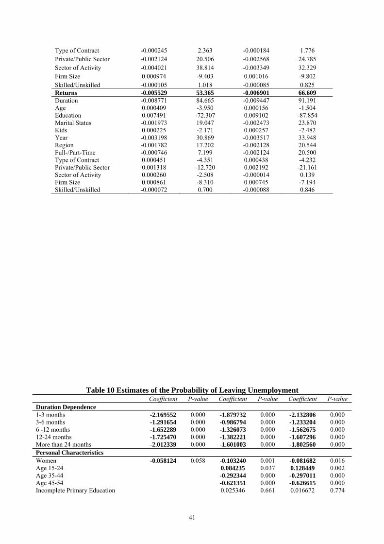
Type of Contract -0.000245 2.363 -0.000184 1.776 Private/Public Sector -0.002124 20.506 -0.002568 24.785 Sector of Activity -0.004021 38.814 -0.003349 32.329 Firm Size 0.000974 -9.403 0.001016 -9.802 Skilled/Unskilled -0.000105 1.018 -0.000085 0.825 Returns -0.005529 53.365 -0.006901 66.609 Duration -0.008771 84.665 -0.009447 91.191 Age 0.000409 -3.950 0.000156 -1.504 Education 0.007491 -72.307 0.009102 -87.854 Marital Status -0.001973 19.047 -0.002473 23.870 Kids 0.000225 -2.171 0.000257 -2.482 Year -0.003198 30.869 -0.003517 33.948 Region -0.001782 17.202 -0.002128 20.544 Full-/Part-Time -0.000746 7.199 -0.002124 20.500 Type of Contract 0.000451 -4.351 0.000438 -4.232 Private/Public Sector 0.001318 -12.720 0.002192 -21.161 Sector of Activity 0.000260 -2.508 -0.000014 0.139 Firm Size 0.000861 -8.310 0.000745 -7.194 Skilled/Unskilled -0.000072 0.700 -0.000088 0.846
Table 10 Estimates of the Probability of Leaving Unemployment Coefficient P-value Coefficient P-value Coefficient P-value
Duration Dependence 1-3 months -2.169552 0.000 -1.879732 0.000 -2.132806 0.000 3-6 months -1.291654 0.000 -0.986794 0.000 -1.233204 0.000 6 -12 months -1.652289 0.000 -1.326073 0.000 -1.562675 0.000 12-24 months -1.725470 0.000 -1.382221 0.000 -1.607296 0.000 More than 24 months -2.012339 0.000 -1.601003 0.000 -1.802560 0.000 Personal Characteristics Women -0.058124 0.058 -0.103240 0.001 -0.081682 0.016 Age 15-24 0.084235 0.037 0.128449 0.002 Age 35-44 -0.292344 0.000 -0.297011 0.000 Age 45-54 -0.621351 0.000 -0.626615 0.000 Incomplete Primary Education 0.025346 0.661 0.016672 0.774
41

Incomplete Secondary Education -0.043091 0.292 -0.041828 0.308 Complete Secondary Education -0.080846 0.082 -0.057888 0.216 Incomplete Tertiary Education 0.087541 0.104 0.111881 0.040 Complete Tertiary Education 0.108170 0.137 0.141806 0.052 Single -0.216943 0.000 -0.196995 0.000 Other Marital Status 0.036458 0.596 0.042200 0.540 Household Characteristics No Kids -0.070735 0.036 -0.072937 0.031 Household Income -0.000076 0.048 -0.000067 0.084 Household Income ^2 (x100) 0.000002 0.020 0.000002 0.023 Economy-wide Characteristics 1995 -0.479600 0.000 -0.477962 0.000 1996 -0.267201 0.000 -0.265506 0.000 1998 0.008356 0.870 0.007468 0.883 1999 -0.143862 0.008 -0.148305 0.006 2000 -0.254717 0.000 -0.265106 0.000 2001 -0.346574 0.000 -0.354496 0.000 Northwest 0.071865 0.104 0.072784 0.100 Northeast 0.200323 0.000 0.214003 0.000 Cuyo 0.399493 0.000 0.373048 0.000 Patagonica 0.447538 0.000 0.433007 0.000 Great Buenos Aires 0.245787 0.000 0.225603 0.000 Last Job Characteristics Agriculture 0.322014 0.002 Manufacturing 0.248890 0.000 Services 0.231434 0.000 N 26927 26927 26927 Log-likilihood -12066.176 -11854.982 -11838.184
Table 11 Estimates of the Probability of Leaving Unemployment Men Women
Coefficient P-value Coefficient P-value Duration Dependence 1-3 months -1.986641 0.000 -2.426308 0.000 3-6 months -0.994879 0.000 -1.679909 0.000 6 -12 months -1.313359 0.000 -2.011870 0.000 12-24 months -1.385437 0.000 -1.996929 0.000 More than 24 months -1.524768 0.000 -2.250930 0.000 Personal Characteristics Women Age 15-24 0.191289 0.000 0.058316 0.363 Age 35-44 -0.349895 0.000 -0.249594 0.002 Age 45-54 -0.769042 0.000 -0.358880 0.001 Incomplete Primary Education -0.023376 0.732 0.139145 0.208
42

Incomplete Secondary Education -0.009401 0.850 -0.081968 0.263 Complete Secondary Education -0.024608 0.681 -0.106379 0.166 Incomplete Tertiary Education 0.080707 0.281 0.109379 0.189 Complete Tertiary Education 0.183443 0.130 0.088413 0.366 Single -0.375118 0.000 0.053107 0.426 Other Marital Status -0.102131 0.433 0.210674 0.016 Household Characteristics No Kids -0.115993 0.007 0.015207 0.784 Household Income -0.000100 0.052 -0.000010 0.873 Household Income ^2 (x100) 0.000001 0.148 0.000002 0.068 Economy-wide Characteristics 1995 -0.542198 0.000 -0.376774 0.000 1996 -0.306122 0.000 -0.221799 0.005 1998 -0.097948 0.139 0.150491 0.061 1999 -0.228788 0.001 -0.021380 0.807 2000 -0.320354 0.000 -0.185225 0.031 2001 -0.364995 0.000 -0.348968 0.000 Northwest 0.022205 0.695 0.151261 0.034 Northeast 0.114792 0.089 0.381336 0.000 Cuyo 0.354762 0.000 0.389978 0.000 Patagonica 0.372148 0.000 0.545804 0.000 Great Buenos Aires 0.23575 0.000 0.196446 0.005 Last Job Characteristics Agriculture 0.27544 0.015 0.615613 0.058 Manufacturing 0.229611 0.000 0.203819 0.037 Services 0.193604 0.002 0.265670 0.000 N 16299 10628 Log-likilihood -7196.161 -4598.065
Table 12 Decomposition of the Gender Gap in Hazard Rates from Unemployment (A) (B) Absolute Value % Absolute Value % Observed Differential -0.009698 100 -0.009698 100 Characteristics -0.000151 1.562 0.003358 -34.625 Duration -0.000001 0.013 0.000262 -2.701 Age -0.000012 0.128 0.000911 -9.397 Education -0.0000003 0.003 0.000385 -3.969 Marital Status -0.000012 0.122 -0.000175 1.806 Kids 0.000001 -0.006 0.000152 -1.564 Household Income -0.000149 1.531 0.002503 -25.804 Year -0.000006 0.062 0.000200 -2.064 Region 0.000015 -0.160 -0.000150 1.544 Sector of Activity 0.000013 -0.132 -0.000730 7.524
43

Returns -0.009547 98.438 -0.013057 134.625 Duration 0.022834 -235.438 0.025406 -261.959 Age -0.000520 5.367 0.000347 -3.576 Education 0.000593 -6.112 0.001316 -13.574 Marital Status -0.009542 98.388 -0.011433 117.882 Kids -0.001944 20.044 -0.001824 18.809 Household Income -0.012965 133.680 -0.018153 187.172 Year -0.004252 43.840 -0.004644 47.883 Region -0.002639 27.211 -0.002282 23.525 Sector of Activity -0.001111 11.458 -0.001791 18.462
Table 13 Unemployed Job Search Methods (%) Men Women Job agency 25.12 27.83 Job Bag 12.73 14.42 Public employment service 7.46 7.8 Answered advertisements 55.54 58.76 Went to firms 67.38 62.07 Looked at advertisements but did not answer 15.93 17.63 Placed advertisements 13.15 15.06 Asked personal contacts 93.17 92.52 Went to places where you knew were hiring people 7.29 4.06 Made negotiations for putting by its own 2.87 1.55 Went to job capacity programs 2.91 3.58 Others (sent curriculums, internet, etc.) 3.62 4.17 Average number of methods 3.07 3.09 Number of observations 2373 1872
B Figures
Figure 1 Male and Female Unemployment Rates in the Great Buenos Aires.
1980-2002. October of each year
44

0
4
8
12
16
20
24
1980
1981
1982
1983
1984
1985
1986
1987
1988
1989
1990
1991
1992
1993
1994
1995
1996
1997
1998
1999
2000
2001
2002
Female unemployment rate Male unemployment rate
Source: Author’s production using data from the INDEC.
Figure 2 Male and Female Unemployment Rates with Ages Ranging from 15 to 19 Years in
the Great Buenos Aires. 1980-2002. October of each year
0
10
20
30
40
50
60
1980
1981
1982
1983
1984
1985
1986
1987
1988
1989
1990
1991
1992
1993
1994
1995
1996
1997
1998
1999
2000
2001
2002
Female unemployment rate Male unemployment rate
Source: Author’s production using data from the INDEC.
Figure 3 Male and Female Unemployment Rates with Ages Ranging from 20 to 34 Years in
the Great Buenos Aires. 1980-2002. October of each year 1980-2002. Octubre de cada año
45
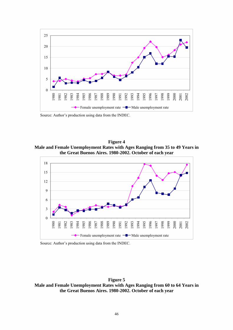
0
5
10
15
20
25
1980
1981
1982
1983
1984
1985
1986
1987
1988
1989
1990
1991
1992
1993
1994
1995
1996
1997
1998
1999
2000
2001
2002
Female unemployment rate Male unemployment rate
Source: Author’s production using data from the INDEC.
Figure 4 Male and Female Unemployment Rates with Ages Ranging from 35 to 49 Years in
the Great Buenos Aires. 1980-2002. October of each year
0
3
6
9
12
15
18
1980
1981
1982
1983
1984
1985
1986
1987
1988
1989
1990
1991
1992
1993
1994
1995
1996
1997
1998
1999
2000
2001
2002
Female unemployment rate Male unemployment rate
Source: Author’s production using data from the INDEC.
Figure 5 Male and Female Unemployment Rates with Ages Ranging from 60 to 64 Years in
the Great Buenos Aires. 1980-2002. October of each year
46

0
4
8
12
16
20
1980
1981
1982
1983
1984
1985
1986
1987
1988
1989
1990
1991
1992
1993
1994
1995
1996
1997
1998
1999
2000
2001
2002
Female unemployment rate Male unemployment rate
Source: Author’s production using data from the INDEC.
Figure 6 Male and Female Labor Force Participation Rates in the Great Buenos Aires.
1980-2002. October of each year
20
24
28
32
36
40
1980
1981
1982
1983
1984
1985
1986
1987
1988
1989
1990
1991
1992
1993
1994
1995
1996
1997
1998
1999
2000
2001
2002
50
52
54
56
58
60
Female participation rate (left axis) Male participation rate (right axis)
Source: Author’s production using data from the INDEC.
Figure 7 Male and Female Labor Force Participation Rates with Ages Ranging from 15 to
19 Years in the Great Buenos Aires. 1980-2002. October of each year
47

15
20
25
30
35
1980
1981
1982
1983
1984
1985
1986
1987
1988
1989
1990
1991
1992
1993
1994
1995
1996
1997
1998
1999
2000
2001
2002
20
30
40
50
Female participation rate (left axis) Male participation rate (right axis)
Source: Author’s production using data from the INDEC.
Figure 8 Male and Female Labor Force Participation Rates with Ages Ranging from 20 to
34 Years in the Great Buenos Aires. 1980-2002. October of each year
45
50
55
60
65
1980
1981
1982
1983
1984
1985
1986
1987
1988
1989
1990
1991
1992
1993
1994
1995
1996
1997
1998
1999
2000
2001
2002
85
90
95
Female participation rate (left axis) Male participation rate (right axis)
Source: Author’s production using data from the INDEC.
Figure 9 Male and Female Labor Force Participation Rates with Ages Ranging from 35 to
49 Years in the Great Buenos Aires. 1980-2002. October of each year
48

35
40
45
50
55
60
65
70
75
1980
1981
1982
1983
1984
1985
1986
1987
1988
1989
1990
1991
1992
1993
1994
1995
1996
1997
1998
1999
2000
2001
2002
95
96
97
98
Female participation rate (left axis) Male participation rate (right axis)
Source: Author’s production using data from the INDEC.
Figure 10 Male and Female Labor Force Participation Rates with Ages Ranging from 50 to
64 Years in the Great Buenos Aires. 1980-2002. October of each year
20
25
30
35
40
45
50
1980
1981
1982
1983
1984
1985
1986
1987
1988
1989
1990
1991
1992
1993
1994
1995
1996
1997
1998
1999
2000
2001
2002
70
75
80
85
90
Female participation rate (left axis) Male participation rate (right axis)
Source: Author’s production using data from the INDEC.
Figure 11 Male and Female Hazard Rates from Employment
49

0.015
0.020
0.025
0.030
0.035
0.040
0.045
0.050
0.055
0.060
1-3 3-6 6-12 12-24 Más de 24
Men Women
Source. Author’s calculations.
Figure 12 Male and Female Hazard Rates from Unemployment
0.07
0.09
0.11
0.13
0.15
0.17
0.19
1-3 3-6 6-12 12-24 Más de 24
Men Women
Source. Author’s calculations.
C Variables
50

Personal Characteristics Unemployed- It is a dummy variable that takes value one if the individual is
unemployed and zero if the individual is employed as a salaried worker.
Women- It is a dummy variable that takes value one if female.
Age- It is measured through four dummies: age 15-24, age 25-34, age 35-44 and age
45-54.
Education- We measure the maximum level of education attained by the individual
through six dummies: incomplete primary studies, complete primary studies, incomplete
secondary studies, complete secondary studies, incomplete tertiary studies and complete
tertiary studies.
Marital Status- We have constructed three dummies: single, that takes value one if the
individual is single, married, that takes value one if the individual is married and other
marital status, that takes value one if the individual is divorced or widow.
Household Characteristics
No Kids- It is a dummy variable that takes value one if the person does not have
children under 14 years.
Household Income- It is obtained summing up the income of each of the other family
members and deflacting it using the Consumer Price Index (base 1999=100).
Economy-wide Characteristics
Region- In order to measure local labor market conditions we have constructed six
dummies: Northwest, Northeast, Cuyo, Pampeana, Patagonica and Great Buenos
Aires28.
Year- In order to take into account the state of the business cycle we have defined seven
dummies: 1995, 1996, 1997, 1998, 1999, 2000 y 2001.
Duration dependence
28 The Northwest region includes Great Catamarca, Great Tucumán-Tafí Viejo, La Rioja, Salta, Jujuy-Palpalá and Santiago del Estero-La Banda. The Northeast region comprises Corrientes, Formosa, Posadas and Great Resistencia. The Cuyo region covers Great Mendoza, San Luis-El Chorrillo and Great San Juan. The Pampeana region includes Great La Plata, Bahía Blanca-Cerri, Great Rosario, Great Santa Fe, Great Paraná, Great Córdoba, Concordia, Santa Rosa-Toay, Mar del Plata-Batán and Río Cuarto. The Patagonica region comprises Comodoro Rivadavia-Rada Tilly, Neuquén-Plottier, Río Gallegos and Ushuaia-Río Grande. Great Buenos Aires includes Ciudad de Buenos Aires and Partidos del Conurbano.
51

Duration-It measures in months the lenght of the spell. It is the sum of three
components: initial duration, that measures in months the time the individual reports to
have been in the state of interest in the first interview; plus six months for each
interview the individual reports to have been in the same state; plus six additional
months minus the time the individual declares to have been in a new state when we
observe a transition. We construct five dummies: 1-3 months, 3-6 months, 6-12 months,
12-24 months, and more than 24 months.
Job Characteristics
Type of Contract-It is measured through three dummies that depend on the employment
type of contract: permanent contract, temporal contract, and other type of contract.
Working Hours-It measures the number of weekly working hours and does not take into
account the extra hours. We have constructed two dummies: part-time, if the person
works less than 35 hours per week, and full-time if the person works more than 35 hours
per week.
Private/Public Sector-We have constructed two dummies: private and public.
Sector of Activity-We have constructed three dummies that groups firms according to
the sector of activity: agriculture,manufacturing, and services.
Level of qualification- We have constructed two dummies related to the third digit of
the National Classification of Occupations: skilled and unskilled.
Firm Size-It is measured through four dummies that classify firms according to the
number of employees: 1-5 employees, 6-25 employees, 26-100 employees and more
than 100 employees.
52