GENERAL I ARTICLE

Efficient Coding of Information: Huffman Coding

Deepak Sridhara

In his classic paper of 1948, Claude Shannon con-sidered the problem of efficiently describing a source that outputs a sequence of symbols, each associated with a probability of occurrence, and provided the theoretical limits of achievable per­formance. In 1951, David Huffman presented a technique that attains this performance. This ar- -==----~-..... ticle is a brief overview of some of their results.

1. Introduction

Shannon's landmark paper 'A Mathematical Theory of Communication' [1] laid the foundation for communica­tion and information theory as they are perceived to­day. In [1], Shannon considers two particular problems: one of efficiently describing a source that outputs a se­quence of symbols each occurring with some probabil­ity of occurrence, and the other of adding redundancy to a stream of equally-likely symbols so as to recover the original stream in the event of errors. The for­mer is known as the source-coding or data-compression problem and the latter is known as the channel-coding or error-control-coding problem. Shannon provided the theoretical limits of coding achievable in both situations, and in fact, he was also the first to quantify what is meant by the "information" content of a source as de­scribed here.

This article presents a brief overview of the source-coding problem and two well-known algorithms that were dis­covered subsequently after [1] that come close to solv­ing this problem. Of particular note is Huffman's algo­rithm that turns out to be an optimal method to rep­resent a source under certain conditions. To state the problem formally: Suppose a source U outputs symbols

Deepak Sridhan worked

as a research associate in

the Deparment of

Mathematics at IISc

between January and

December 2004. Since

January 2005, he has been

a post-doctoral research

associate in the Institute

for Mathematics at

U nviersity of Zurich. His

research interests include

coding theory, codes over

graphs and iterative

techniques, and informa­

tion theory.

Keywords Entropy, source coding, Huff­man coding.

-RE-S-O-N-A-N-C-E-I--Fe-b-rU-a-rY--2-00-6-----------~------------------------------~

1 By a D-ary string we mean a sequence (yl'y2 •...• y,) where each y, belongs to the set {O.1.2 •...• D-l}.

Intuitively, the optimal

number of bits needed

to represent a source

symbol uj with

probability of

occurrence Pi is

around 1092 11Pi bits.

GENERAL I ARTICLE

problem formally: Suppose a source U outputs symbols Ul, U2, ,UK, belonging to some discrete alphabet U, with probabilities P(Ul),P(U2), ,P(UK), respectively. The source-coding problem is one of finding a mapping from U to a sequence of D-ary strings!, called code­words, such that this mapping is invertible. For the coding to be efficient, the aim is to find an invertible mapping (or, a code) that has the smallest possible av­erage codeword-length (or, code-length). By the way this problem is stated, a source U can also be treated as a discrete random variable U that takes values from U = {Ul' U2, ,UK} and that has a probability distri­bution given by p(U), where p(U = Ui) = P(Ui), for i=1,2, K

As an example, suppose a random variable U takes on four possible values Ul, U2, U3, U4 with probability of oc­currences p( Ul) = t, p( U2) = ~,p( U3) = k, p( U4) = k· A naive solution for representing the symbols Ul, ,U4

in terms of binary digits is to represent each symbol using two bits: Ul = 00, U2 = 01, U3 = 10, U4 = 11. The average code-length in this representation is two bits. However, this representation turns out to be a sub-optimal one. An efficient representation uses fewer bits to represent symbols occurring with a higher prob­ability and more bits to represent symbols occurring with a lower probability. An optimal representation for this example is Ul = 0, U2 = 10, U3 = 110, U4 = 111. The average code-length in this representation is 1· t+2' ~+3· k+3' k = 1.75 bits. Intuitively, the optimal number of bits needed to represent a source symbol Ui

with probability of occurrence Pi is around log2 ;i bits. Further, since Ui occurs with probability Pi, the effec­tive code-length of Ui in such a code is Pi log2 p~. Shan­non's idea was to quantify the 'information' content of a source or random variable U in precisely these terms. Shannon defined the entropy of a source U to measure its information content, or equivalently, the entropy of

5 -2---------------------------~-----------R-E-SO-N-A-N-C-E--I-Fe-b-ru-a-rY--2-00-6

GENERAL I ARTICLE

a random variable U to measure its 'uncertainty', as H (U) = Li Pi log2 ;i' The coding techniques discussed in this article are evaluated using this measure of 'infor­mation' content.

This article is organized as follows. Section 2 introduces some definitions and notation that will be used in this paper. Section 3 provides the notion of typical sequences that occur when a sequence of independent and identi­cally distributed random variables are considered. This section also states the properties of typical sequences which are used to prove the achievability part of Shan­non's source-coding theorem, in Section 4. Section 5 introduces the notion of D-ary trees to illustrate the en­coding of a source into sequences of D-ary alphabets. Another version of the source-coding theorem for the special case of prefix-free codes is presented here. A coding technique, credited to Shannon and Fano, which is a natural outcome of the proof of the source-coding theorem stated in Section 5, is also presented. Sec­tion 6 presents Huffman's optimal coding algorithm that achieves a lower average code-length than the Shannon­Fano algorithm. The paper is concluded in Section 7.

2. Preliminaries

Some basic definitions and notation that will be used in this article are introduced here.

Let X be a discrete random variable taking values in a finite alphabet X. For each x E X let p(x) denote the probability that the random variable X takes the value x written as Pr(X = x).

Definition 2.1. The expectation of a function J(X) de­fined over the random variable X is defined by

E[f(X)] = L J(x)p(x) xEX

Definition 2.2. The entropy H(X) of a discrete random

Shannon defined the

entropy of a source U

to measure its

information content,

or equivalently, the

entropy of a random

variable U to measure

its 'uncertainty', as

H(U)=LiPi 1092 11Pr

--------~--------RESONANCE I February 2006 53

The entropy H(X) of a

discrete random

variable X is defined

by H(X) = -L p(x) log p(x).

xe.'C

GENERAL I ARTICLE

variable X is defined by

H(X) = - LP(x) logp(x). xEX

To avoid ambiguity, the term p( x) log p( x) is defined to be 0 when p( x) = O. By the previous definition, H (X) = -E[logp(X)]. For most of the discussion, we will use logarithms to the base 2, and therefore, the entropy is measured in bits. (However, when we use logarithms to the base D for some D > 2, the corresponding entropy of X is denoted as H D (X) and is measured in terms of D-ary symbols.) Note that in the above expression, the summation is over all possible values x assumed by the random variable X, and p(x) denotes the corresponding probability of X = x.

We will use uppercase letters to indicate random vari­ables, lowercase letters to indicate the actual values as­sumed by the random variables, and script-letters (e.g., X) to indicate alphabet sets. The probability distribu­tion of a random variable X will be denoted by p( X) or simply p.

Extending the above definition to two or more random variables, we have

Definition 2.3. The joint entropy of a vector of random variables (Xl, X 2, ,Xn ) is defined by

where P(XI' X2, . x n ) = Pr(X I = Xl, X 2 = x2,

x n ).

Definition 2.4. (a) A collection of random variables {Xl, X 2 , . Xn} with Xi taking values from an alphabet X is called independent if for any choice {Xl, X2, . Xn}

5 -4----------------------------~-----------R-ES-O-N-A-N-C-E-I-F-e-br-ua-r-Y-2-0-06

GENERAL I ARTICLE

with Xi = Xi, i == 1,2, . n, the probability of the joint event {Xl = Xb ,Xn == xn} equals the product n~=l Pr(Xi == Xi).

(b) A collection of random variables {Xl, X 2 ,· . Xn} is said to be identically distributed if Xi = X: that is, all the alphabets are the same, and the probability Pr(Xi = x) is the same for all i.

( c) A collection of random variables {X I, X 2, . X n} is said to be independent and identically distributed (i.i.d.) if it is both independent and identically distributed.

An important consequence of independence is that if {Xb X 2 , . Xn} are independent random variables, each taking on only finitely many values, then for any func­tion fi(')' i = 1,2, . n,

n n

E[II fi(Xi)] == II E[fi(Xi)], i=l i=l

Thus if {Xl, X 2 , . Xn} are independent and take values over finite alphabets, then the entropy

n n

L E[logp(Xi)] == L H(Xi)' i=l i=l

If, in addition, they are identically distributed, then

Note that if Xl, ,Xn are a sequence of i.i.d. random variables as above, then their joint entropy is H(X b X 2 ,

,Xn ) == nH(X).

Definition 2.5. A sequence {Yn } of random variables is said to converge to a random variable Y in probability if for each E > °

Pr(IYn - YI > E) ----+ 0, as n ----+ 00,

A collection of

random variables

{Xl' X2, ... , X,J is said

to be identically

distributed if X;=X:

that is, all the

alphabets are the

same, and the

probability Pr(X;=x) is

the same for all i.

-RE-S-O-N-AN-C-E--I-Fe-b-rU-a-rY--20-0-6---------~----------------------------55

The assertion that

X n ~ E[X1] with

probability one is

called the strong law

of large numbers and

the assertion that

Xn~ E[X1] in

probability is called

the weak law of large

numbers.

GENERAL I ARTICLE

and with probability one if

Pr (lim Yn = Y) = 1. n-co

It can be shown that if Yn converges to Y with probabil­ity one, then Yn converges to Y in probability, but the converse is not true in general.

The law of large numbers (LLN) of probability theory says that the sample mean Xn == lin L:~=1 Xi of n i.i.d. random variables {Xb X 2 , . Xn} gets close to m = E[Xil as n gets very large. More precisely, it says that X n converges to E [X 1] with probability 1 and hence in probability. Here we are considering only the case when the random variables take on finitely many values. The LLN is valid for random variables taking infinitely many values under some appropriate hypothesis (see R L Karandikar [4]). The assertion that Xn ~ E[X 1] with probability one is called the strong law of large numbers and the assertion that Xn ~ E[X1] in probability is called the weak law of large numbers. See Karandikar [4] and Feller [5] for extensive discussions (including proofs) on both the weak law and the strong law of large num­bers.

3. Typical Sets and the Asymptotic Equiparti­tion Theorem

As a consequence of the law of large numbers, we have the following result:

Theorem 3.1. If X 11 X 2, are independent and identi­cally distributed (i.i.d.) random variables with a prob­ability distribution p(.), then

with probability 1.

Proof. Since Xl) ) Xn are i.i.d. random variables,

-56----------------------------~-----------R-E-S-O-NA-N-C-E--IF-e-br-u-ar-Y-2-0-06

GENERAL I ARTICLE

converges to -E[logp(X)] = H(X) with probability 1 as n ~ 00, by the strong law of large numbers. •

This theorem says that the quantity * log P(Xl,X~ ... ,Xn) is close to the entropy H(X) when n is large. Therefore, it makes sense to divide the set of sequences (Xl1 X2, ,xn )

E xn into two sets: the typical set wherein each se­quence (Xb X2, ,xn ) is such that ~ log p(xI.~ .. ,xn) is close to the entropy H(X) and the non-typical set containing

sequences with * log P(Xl'~"'Xn) bounded away from the entropy H (X). As n increases, the probability of se­quences in the typical set becomes high.

Definition 3.1. For each € > 0, let A~n) be the set of sequences (Xl, X2, ,Xn) E xn with the following prop­erty:

Call A~n) a typical set.

Theorem 3.2. Fix E > O. For A~n) as defined above the following hold:

1. If (Xl' x2,

log p( xl, X2,

,Xn) E A~n), then H(X) - E ~ -~ ,xn)~H(X)+E.

2. If {X 11 X 2, . X n} are i.i.d. with probability dis-

tribution p(X) then Pr((xb X2, . xn) E A~n») == Pr(A~n») ---+ 1 as n ---+ 00.

3. IA~n) I ~ 2n(H(X)+€) , where for any set S, lSI is the number of elements in S.

4. IA~n)1 ~ (1 - E)2n(H(X)-€) for n sufficiently large.

-RE-S-O-N-AN-C-E--I-Fe-b-rU-a-rY--20-0-6---------~~-------------------------~-

Shannon's source­

coding theorem

states that to

describe a source

by a code C, on an

average at least

H(X) bits (or, D-ary

symbols) are

required.

GENERAL I ARTICLE

Proof. The proof of (1) follows from the definition of A~n) and that of (2) from Theorem 3.l.

To prove (3), we observe that the following set of equa­tions hold:

1 = L P(Xb ,Xn ) 2:: L P(Xl' (Xl, .. ·,Xn)EXn

(Xl, ... ,Xn)EA~n)

>

To prove (4), note by (2) that for n large enough

This means that

x ) E A (n)) = ,n e

L P(Xl' X2, xn) (Xl, ... ,Xn)EA~n)

::; 2-n(H(X)-e) IA~n) I.

• 4. Source Coding Theorem

Shannon's source-coding theorem states that to describe a source by a code C, on an average at least H (X) bits (or, D-ary symbols) are required. The theorem further states that there exist codes that have an expected code­length very close to H (X). The following theorem shows the existence of codes with expected code-length close to the source entropy. This theorem can also be called the achievability-part of Shannon's source-coding theo­rem, and says that the average number of bits needed to represent a symbol x from the source is H (X), the entropy of the source.

5 -8----------------------------~~---------R-ES-O-N-A-N-C-E-I-F-e-br-u-ar-Y-Z-O-06

GENERAL I ARTICLE

Non-typical set

Typical set (n) ( ~, AE

: ';!l H+ ~ elements

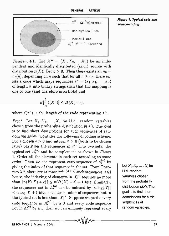
Theorem 4.1. Let xn = (Xl, X 2 , . Xn) be an inde­pendent and identically distributed (i.i.d.) source with distribution p(X). Let 1] > O. Then there exists an no = no( 1]), depending on 1] such that for all n ~ no, there ex­ists a code which maps sequences xn = (Xb X2, ,xn)

of length n into binary strings such that the mapping is one-to-one (and therefore invertible) and

where f(xn) is the length of the code representing xn.

Proof. Let X 1l X 2 , ,Xn be i.i.d. random variables chosen from the probability distribution p( X). The goal is to find short descriptions for such sequences of ran­dom variables. Consider the following encoding scheme: For a chosen € > 0 and integer n > 0 (both to be chosen later) partition the sequences in xn into two sets: the typical set A~n) and its complement as shown in Figure 1. Order all the elements in each set according to some order. Then we can represent each sequence of A~n) by giving the index of that sequence in the set. From Theo­rem 3.2, there are at most 2n (H(X)+«o) such sequences, and hence, the indexing of elements in A~n) requires no more than r n(H(X) + €)l ::; n(H(X) + €) + 1 bits. Similarly, the sequences not in A~n) can be indexed by r n log /Xil ::; n log I X 1+ 1 bits since the number of sequences not in the typical set is less than /Xl n Suppose we prefix every code sequence in A~n) by a 0 and every code sequence not in A~n) by a 1, then we can uniquely represent every

Figure 1. Typical sets and source-codlng.

Let X11 X21 •• , ,Xn be

LLd. random

variables chosen

from the probability

distribution p(X). The

goal is to find short

descriptions for such

sequences of

random variables.

-RE-S-O-N-A-N-C-E-I-F-e-br-U-ar-Y-2-0-0-6----------~--------------------------59

The converse to the

source-coding

theorem states that

every code that

maps sequences of

length n from a

source X into binary

strings, such that the

mapping is one-to­

one, has an average

code length that is at

least the entropy

H(X).

GENERAL I ARTICLE

sequence of length n from xn. The average length of codewords in such an encoding scheme is given by

L p(xn)[n log IXI + 2] xnExn-A~n)

= Pr{A~n)}[n(H(X)+E)+2]+(1-Pr{A~n)})[n log IXI+2] = Pr{A~n)}[n(H(X) +E)] +(1- Pr{A~n)})[n log IXI] +2.

By (2) of Theorem 3.2, there exists a nO(E) such that for n ;::: nO(E), 1 - Pr(A~n») < E. Thus

E[l(xn)] ~ n(H(X)+E)+nE(1og IXI)+2 = n(H(X)+€').

where E' == €+€ log IXI +~. Given 1] > 0 choose an € and no(€) large enough such that €' < 1]. Since the choice of € depends on 1], no( €) can be written as no( 1]). •

The above result proves the existence of a source-coding scheme which achieves an average code length of (H(X)+ €'). However, this proof is non-constructive since it does not describe how to explicitly find such a typical set. The converse to the source-coding theorem states that every code that maps sequences of length n from a source X into binary strings, such that the mapping is one­to-one, has an average code length that is at least the entropy H (X). We will prove another version of this result in the following section by restricting the coding to a special class of codes known as prefix-free codes.

5. Efficient Coding of Information

The notion of trees is introduced to illustrate how a code, that maps a sequence of symbols from a source X

-60--------------------------VV\Afvv----------R-ES-O-N-A-NC-E--'-Fe-b-rU-ar-y-2-00-6

GENERAL I ARTICLE

Q : f 0 1 0

2 0 •

1 1 ~ - 1

2 ~ () -

2 1

2 2 -

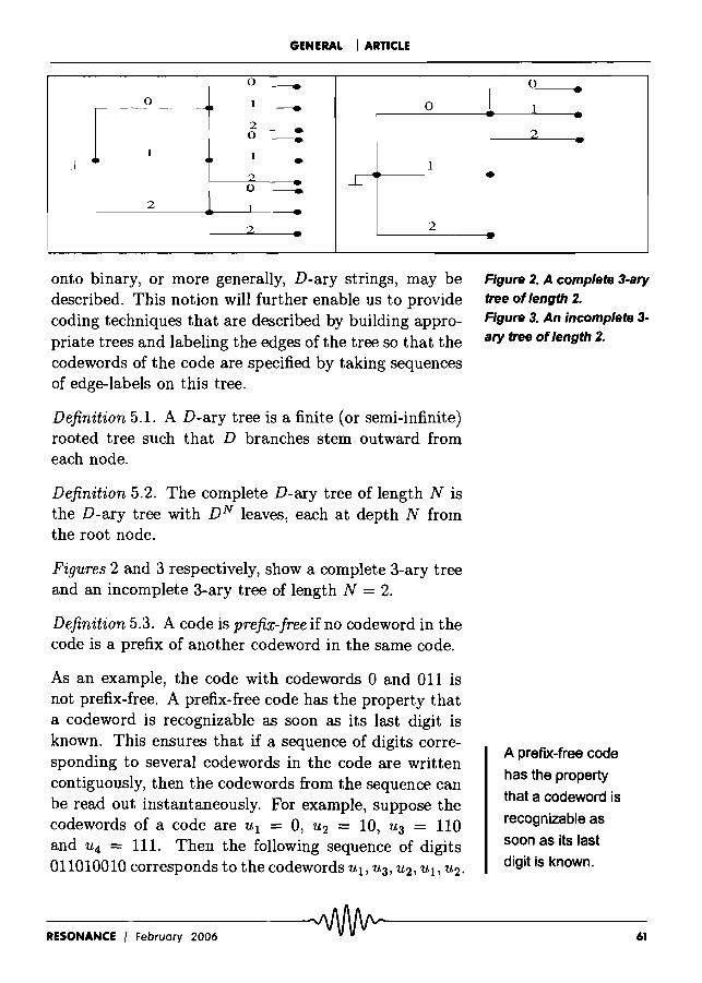
onto binary, or more generally, D-ary strings, may be described. This notion will further enable us to provide coding techniques that are described by building appro­priate trees and labeling the edges of the tree so that the codewords of the code are specified by taking sequences of edge-labels on this tree.

Definition 5.1. A D-ary tree is a finite (or semi-infinite) rooted tree such that D branches stem outward from each node.

Definition 5.2. The complete D-ary tree of length N is the D-ary tree with DN leaves, each at depth N from the root node.

Figures 2 and 3 respectively, show a complete 3-ary tree and an incomplete 3-ary tree of length N = 2.

Definition 5.3. A code is prefix-free if no codeword in the code is a prefix of another codeword in the same code.

As an example, the code with codewords 0 and 011 is not prefix-free. A prefix-free code has the property that a codeword is recognizable as soon as its last digit is known. This ensures that if a sequence of digits corre­sponding to several codewords in the code are written contiguously, then the codewords from the sequence can be read out instantaneously. For example, suppose the codewords of a code are Ul = 0, U2 = 10, U3 = 110 and U4 = 111. Then the following sequence of digits 011010010 corresponds to the codewords Ull U3, U2, Ull U2.

0 -1 --2 -

-

--Figure 2. A complete 3-ary tree of length 2. Figure 3. An incomplete 3-ary tree of length 2.

A prefix-free code

has the property

that a codeword is

recognizable as

soon as its last

digit is known.

-RE-S-O-N-A-N-C-E-I-F-e-br-U-ar-Y-2-0-0-6----------~-----------------------------~

There exists a D­

ary prefix-free

code whose code­

lengths are the

positive integers

W1,W2, ••• ,WK if and

only if

"i.i=t a-w. ~ 1.

GENERAL I ARTICLE

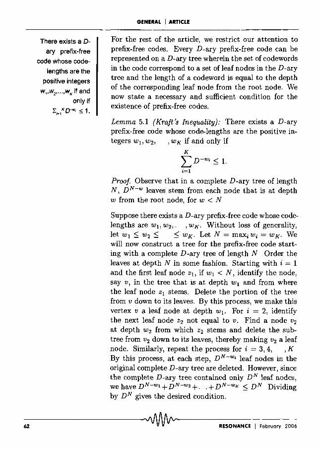
For the rest of the article, we restrict our attention to prefix-free codes. Every D-ary prefix-free code can be represented on a D-ary tree wherein the set of codewords in the code correspond to a set of leaf nodes in the D-ary tree and the length of a codeword is equal to the depth of the corresponding leaf node from the root node. We now state a necessary and sufficient condition for the existence of prefix-free codes.

Lemma 5.1 (Kraft's Inequality): There exists a D-ary prefix-free code whose code-lengths are the positive in-tegers Wll W2, ,WK if and only if

K

LD-Wi ~ 1. i=1

Proof. Observe that in a complete D-ary tree of length N, DN -w leaves stem from each node that is at depth W from the root node, for w < N

Suppose there exists a D-ary prefix-free code whose code­lengths are Wb W2, . , WK. Without loss of generality, let WI ~ W2 ~ ~ WK. Let N = maxi Wi = WK. We will now construct a tree for the prefix-free code start­ing with a complete D-ary tree of length N Order the leaves at depth N in some fashion. Starting with i = 1 and the first leaf node ZI, if WI < N, identify the node, say v, in the tree that is at depth WI and from where the leaf node ZI stems. Delete the portion of the tree from v down to its leaves. By this process, we make this vertex v a leaf node at depth WI. For i = 2, identify the next leaf node Z2 not equal to v. Find a node V2

at depth W2 from which Z2 stems and delete the sub­tree from V2 down to its leaves, thereby making V2 a leaf node. Similarly, repeat the process for i = 3,4, ,K By this process, at each step, DN -Wi leaf nodes in the original complete D-ary tree are deleted. However, since the complete D-ary tree contained only DN leaf nodes, wehaveDN- w l+DN-w 2+ .. +DN-WK ~ DN Dividing by DN gives the desired condition.

6-2---------------------------~-----------R-ES-O-N-A-N-C-E--I-Fe-b-ru-o-rY--2-0o-6

GENERAL I ARTICLE

To prove the converse, suppose Wb W2, , W K are pos­itive integers satisfying the inequality l:~1 D-Wi ::; 1 (*). Then, without loss of generality, let WI ::; W2 ::;

~ WK. Set N = maXi Wi = WK. We want to show that we are able to construct a prefix-free code with codeword lengths WI, W2, ,WK' Start again with the complete D-ary tree.

Let i = 1. Identify a node Zl at depth WI to be the first codeword of the code we intend to construct. If WI < N, delete the subtree stemming from Zl down to its leaves so that Zl becomes a leaf node. Next, increment i by 1 and look for a node Zi in the remaining tree which is not a codeword and is at depth Wi. If there is such a node, call this the ith codeword and delete the subtree stemming from Zi down to its leaves. Repeat the above process by incrementing i by 1. This algorithm terminates when either i > K or when the algorithm cannot find a node Zi

satisfying the desired property in the ith step for i ::; K

If the algorithm identifies K codeword nodes, then a prefix-free code can be constructed by labeling the edges of the tree as follows: At each node, label the r ::; D edges that stem from it as 0,1,2. ,r - 1 in any order. The ith codeword is then the sequence of edge-labels from the root node up to the ith codeword node.

The only part remaining to be seen is that the above algorithm will not terminate before K codeword nodes have been identified. To show this, consider the ith step of this algorithm when ZI, Z2, 'Zi-l have been identi­fied and Zi needs to be chosen. The number of surviving leaves at depth N not stemming from any codeword is DN - (DN-Wl + DN-w2 + + DN-Wi-l). But by our assumption (*), this number is greater than zero. Thus, there exists a node Zi which is not a codeword and which is at depth Wi in the tree that remains at step i. Further­more, since Wi 2:: Wi-l 2:: Wi-2 2:: WI, the node Zi will not lie in any of the paths from the root node to any of

If the algorithm

identifies K codeword

nodes, then a prefix­

free code can be

constructed by

labeling the edges of

the tree as follows: At

each node, label the r

~ D edges that stem

from it as 0,1,2 ... , r-1

in any order. The i th

codeword is then the

sequence of edge­

labels from the root

node up to the i th

codeword node.

-RE-S-O-N-A-N-CE--I-F-eb-r-Ua-rY--2-00-6-----------~---------------------------~-

The depth of a

codeword-node is

equal to the length of

the codeword in the

code,andthe

codeword is the

sequence of edge­

labels on this tree

from the root node up

to the corresponding

codeword-node.

GENERAL I ARTICLE

Zl, z2 ,Zi-l. This argument holds for i = 1,2, ,K; hence, this algorithm will always be able to identify K codeword nodes and construct the corresponding prefix­free code. •

A. Trees with Probability Assignments

Let us suppose that there is a D-ary prefix-free code that maps symbols from a source U onto D-ary strings such that the mapping is invertible. For convenience, let Ul, U2, , UK be the source symbols and let the code­words corresponding to these symbols also be denoted by Ub U2, ,UK. The proof of the Kraft inequality tells us how to specify a D-ary prefix-free code on a D-ary tree. That is, a D-ary tree can be built with the edges labeled as in the proof of Lemma 5.1 such that the code­words are specified by certain leaf nodes on this tree, the depth of a codeword-node is equal to the length of the codeword in the code, and the codeword is the sequence of edge-labels on this tree from the root node up to the corresponding codeword-node. Furthermore, probabili­ties can be assigned to all the nodes in the tree as fol­lows: assign the probability P(Ui) for the codeword node which corresponds to the codeword Ui (or, the source symbol Ui.) Assign the probability zero to a leaf node that is not a codeword node. Assign a parent node (that is not a leaf node), the sum of the probabilities of its children nodes. It is easy to verify that for such an as­signment, the root node will always have a probability equal to 1. Such a D-ary tree gives a complete descrip­tion of the D-ary prefix-free code. This description will be useful in describing two specific coding methods: the Shannon-Fano coding algorithm and the Huffman cod­ing algorithm.

B. Source Coding Theorem for Prefix-Free Codes

Before we present the two coding techniques, we present another version of the source-coding theorem for the

-M----------------------------~~---------RE-S-O-N-AN-C-E--I -Fe-b-rU-ary 2006

GENERAL I ARTICLE

special case of prefix-free codes:

Theorem 5.1. Let ii, i;, ,i:n be the optimal codeword lengths for a source with distribution p(X) and a D­ary alphabet, and let L* be the corresponding expected length of the optimal prefix-free code (L* = ~i Piir). Then

Proof. We first show that the expected length L of any prefix-free D-ary code for a source described by the ran­dom variable X with distribution p(X) is at least the en­tropy H D(X). To see this, let the code have codewords of length ill i 2 , and let the corresponding probabil­ities of the codewords be Pl, P2, .. Consider the dif­ference between the expected length L and the source entropy HD(X),

L - HD(X) = LPiii - LPilogD ~ i i Pl

= - LPilogDD-li + LPilogDPi. i i

The first term on the right-hand side is a well-known term in information theory, called the 'divergence' be­tween the probability distributions rand P can be shown to be non-negative. (See [2]). The second term is also non-negative since c :::; 1 by the Kraft inequality. This shows that L - HD(X) ~ o. Suppose there is a prefix-free code with codeword lengths ill i 2 , such that ii = rlogD ;J. Then the ii's satisfy

the Kraft inequality since ~i D-li :::; L:i Pi = 1. Fur­thermore, we have

1 1 logD - :::; £i :::; logD - + 1.

Pi Pi

The expected

length L of any

prefix-free D-ary

code for a source

described by the

random variable X

with distribution

p(X) is at least the

entropy H D(X).

--------~--------RESONANCE I February 2006 65

This theorem says

that an optimal

code will use at

most one bit more

than the source

entropy to describe

the source

alphabets.

GENERAL I ARTICLE

Hence, the expected length L of such a code satisfies

Since an optimal prefix-free code can only be better than the above code, the expected length L * of an optimal code satisfies the inequality L * ~ L ~ H D (X) + 1. Since we have already shown that any prefix-free code must have an expected length which is at least the entropy, this proves that

HD(X) ~ L* ~ HD(X) + 1. • Note that in the above theorem, we are trying to find a description of all the alphabets of the source individu­ally. This theorem says that an optimal code will use at most one bit more than the source entropy to describe the source alphabets. In order to achieve a better com­pression, we can find a corresponding code for a new source whose alphabets are sequences of length n > 1 of the original source X. As n gets larger, the correspond­ing optimal code will have an effective code-length as close to its source entropy as possible. In fact, it can be shown that the effective code-length for an optimal code then satisfies H(X) ~ E[~xn]* ~ H(X) +~. This result is in accordance with Theorem 4.1 of Section 4.

c. Shannon-Fano Prefix-Free Codes

Following the proof-technique of Theorem 5.1, we present a natural source-coding algorithm that is popularly kn­own as the Shannon-Fano algorithm. For a source U, this algorithm constructs D-ary prefix-free codes with expected length at most one more than the entropy of the source. The algorithm is as follows:

-66----------------------------~-----------R-ES-O-N-A-N-C-E-I-F-e-br-u-ar-Y-Z-O-06

GENERAL I ARTICLE

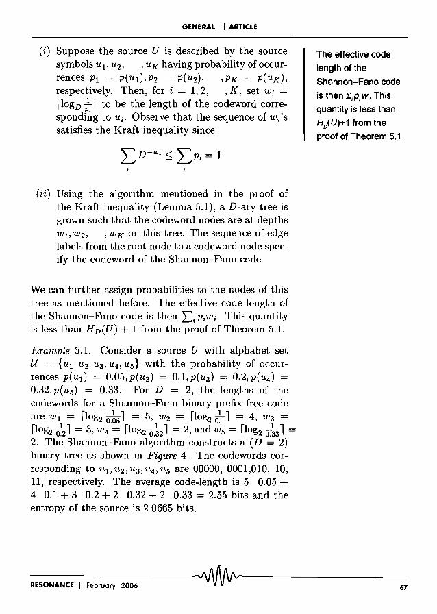
(i) Suppose the source U is described by the source symbols Ub U2, ,UK having probability of occur-rences PI = P(UI),P2 = P(U2), ,PK = P(UK), respectively. Then, for i = 1,2, ,K, set Wi =

flogD ;i 1 to be the length of the codeword corre­sponding to Ui. Observe that the sequence of wi's satisfies the Kraft inequality since

L D - Wi ~ LPi = 1. i i

(ii) Using the algorithm mentioned in the proof of the Kraft-inequality (Lemma 5.1), a D-ary tree is grown such that the codeword nodes are at depths WI, W2, ,'WK on this tree. The sequence of edge labels from the root node to a codeword node spec­ify the codeword of the Shannon-Fano code.

We can further assign probabilities to the nodes of this tree as mentioned before. The effective code length of the Shannon-Fano code is then L:i PiWi' This quantity is less than HD(U) + 1 from the proof of Theorem 5.1.

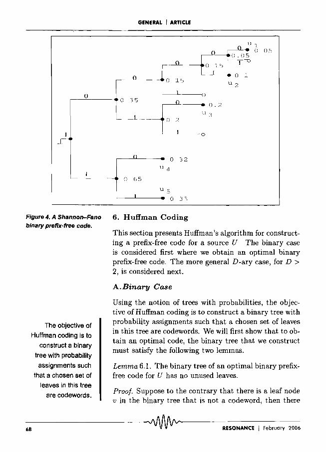
Example 5.1. Consider a source U with alphabet set U = {Ub U2, U3, U4, U5} with the probability of occur­rences P(UI) = 0.05,P(U2) = 0.I,p(u3) = 0.2,P(U4) = 0.32, p( U5) = 0.33. For D = 2, the lengths of the codewords for a Shannon-Fano binary prefix free code are w\ = rlog2 0.~51 = 5, W2 = rlog2 0\ 1 = 4, W3 = flOg2 0.21 = 3, W4 = flog2 0.~21 = 2, and W5 = flog2 0.~31 = 2. The Shannon-Fano algorithm constructs a (D = 2) binary tree as shown in Figure 4. The codewords cor­responding to Ub U2, U3, U4, U5 are 00000, 0001,010, 10, 11, respectively. The average code-length is 5 0.05 + 4 0.1 + 3 0.2 + 2 0.32 + 2 0.33 = 2.55 bits and the entropy of the source is 2.0665 bits.

The effective code

length of the

Shannon-Fanocode

is then L;P;W;, This

quantity is less than

HD(U)+1 from the

proof of Theorem 5.1 .

________ .AAAAA~ ______ _ RESONANCE I February 2006 v V V V V V'"" 67

GENERAL I ARTICLE

o _U l OS Q 1 - ° rO.O S

{)

° lS 1 v

1 - ° l 0

° lS u2

0 ~ 0

0 3S 0

10

• 0.2

1 u 3

2

I ] 0

~----4.

0 - ° 32 -u 4

1

° 6S

Us ] • 0 33

Figure4.AShannon-Fano 6. Huffman Coding binary prefix-free code.

The objective of

Huffman coding is to

construct a binary

tree with probability

assignments such

that a chosen set of

leaves in this tree

are codewords.

This section presents Huffman's algorithm for construct­ing a prefix-free code for a source U The binary case is considered first where we obtain an optimal binary prefix-free code. The more general D-ary case, for D > 2, is considered next.

A.Binary Case

Using the notion of trees with probabilities, the objec­tive of Huffman coding is to construct a binary tree with probability assignments such that a chosen set of leaves in this tree are codewords. We will first show that to ob­tain an optimal code, the binary tree that we construct must satisfy the following two lemmas.

Lemma 6.1. The binary tree of an optimal binary prefix­free code for U has no unused leaves.

Proof. Suppose to the contrary that there is a leaf node v in the binary tree that is not a codeword, then there

-68-----------------------------~-----------R-E-SO-N-A-N-C-E--1 -Fe-b-ru-a-rY--2-00-6

GENERAL I ARTICLE

is a parent node v' that has v as its child node. Since the tree is binary, v has another child node u. Suppose u is a codeword node corresponding to the codeword c, then deleting U and v and representing v' as the codeword node c yields a code with a lower average code-length since we have reduced the code-length for the codeword c without affecting the code lengths of the remaining codewords. However, since we assumed that the binary tree represented an optimal code to begin with, this is a contradiction. •

Lemma 6.2. There is an optimal binary prefix-free code for U such that the two least likely codewords, say UK-l

and UK, differ only in their last digit.

Proof. Suppose we have the binary tree for an optimal code. Let Ui be one of the longest codewords in the tree. By Lemma 6.1, there are no unused leaves in this tree, so there is another codeword Uj which also has the same parent node as Ui. Suppose Uj =/:. UK, then we can inter­change the codeword nodes for Uj and UK' This inter­change will not increase the average code-length since P(UK) :::; p(Uj) and since the code-length of UK is at least the code-length of Uj in the original code. Now if Ui =/:. UK -1, we can similarly interchange the codeword nodes for Ui and UK-I' Thus, the new code has UK and UK-1 among its longest codewords and UK and UK-1

are connected to the same parent node. Since the code­words are obtained by the sequence of edge-labels from the root node up to the corresponding codeword nodes, the codewords for UK and UK -1 differ only in their last digit. •

The above two lemmas suggest that to construct an op­timal binary tree, it is useful to begin with the two least likely codewords. Assigning these two codewords as leaf nodes that are connected to a common parent node gives part of the tree for the optimal code. The parent node is now considered as a codeword having a probability that

The above two

lemmas suggest

that to construct an

optimal binary tree,

it is useful to begin

with the two least

likely codewords.

-RE-S-O-N-A-N-C-E-I-F-e-br-U-ar-Y-2-0-0-6----------~----------------------------6-9

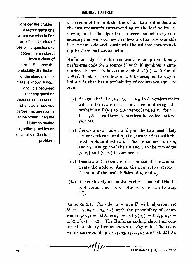
Consider the problem

of twenty questions

where we wish to find

an efficient series of

yes-or-no questions to

determine an object

from a class of

objects. Suppose the

probability distribution

of the objects in this

class is known a priori

and it is assumed

that any question

depends on the series

of answers received

before that question is

to be posed, then the

Huffman coding

algorithm provides an

optimal solution to this

problem.

GENERAL I ARTICLE

is the sum of the probabilities of the two leaf nodes and the two codewords corresponding to the leaf nodes are now ignored. The algorithm proceeds as before by con­sidering the two least likely codewords that are available in the new code and constructs the subtree correspond­ing to these vertices as before.

Huffman's algorithm for constructing an optimal binary prefix-free code for a source U with K symbols is sum­marized below. I t is assumed that P ( u) i= 0 for all u E U. That is, no codeword will be assigned to a sym­bol u E U that has a probability of occurrence equal to zero.

(i) Assign labels, i.e., Ul, U2, ,UK to K vertices which will be the leaves of the final tree, and assign the probability P(Ui) to the vertex labeled Ui, for i = 1, , K Let these K vertices be called 'active' vertices.

(ii) Create a new node v and join the two least likely active vertices Ui and Uj (Le., two vertices with the least probabilities) to v. That is connect v to Ui

and Uj. Assign the labels 0 and 1 to the two edges (v, Ui) and (v, Uj) in any order.

(iii) Deactivate the two vertices connected to v and ac­tivate the node v. Assign the new active vertex v the sum of the probabilities of Ui and Uj.

( i v) If there is only one active vertex, then call this the root vertex and stop. Otherwise, return to Step (ii).

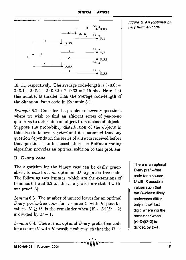
Example 6.1. Consider a source U with alphabet set U = {uJ, U2, U3, U4, us} with the probability of occur­rences p(ud = 0.05, P(U2) = 0.1,p(u3) = 0.2,P(U4) = 0.32, p( us) = 0.33. The Huffman coding algorithm con­structs a binary tree as shown in Figure 5. The code­words corresponding to Ul, U2, U3, U4, Us are 000, 001,01,

7 -O----------------------------~-----------R-ES-O-N-A-N-CE--I-F-eb-r-ua-r-Y-Z-O-06

GENERAL I ARTICLE

n U l

1 - 0.05 0 r 0.15

J U 2

- 0.1 0

0.35

1 U 3

- 0.2 ~~ 1

0 0.32

1 U 4

0.65

1 Us - 0.33

10,11, respectively. The average code-length is 3·0.05+ 3·0.1 + 2·0.2 + 2·0.32 + 2 0.33 = 2.15 bits. Note that this number is smaller than the average code-length of the Shannon-Fano code in Example 5.l.

Example 6.2. Consider the problem of twenty questions where we wish to find an efficient series of yes-or-no questions to determine an object from a class of objects. Suppose the probability distribution of the objects in this class is known a priori and it is assumed that any question depends on the series of answers received before that question is to be posed, then the Huffman coding algorithm provides an optimal solution to this problem.

B. D-ary case

The algorithm for the binary case can be easily gener­alized to construct an optimum D-ary prefix-free code. The following two lemmas, which are the extensions of Lemmas 6.1 and 6.2 for the D-ary case, are stated with­out proof [3].

Lemma 6.3. The number of unused leaves for an optimal D-ary prefix-free code for a source U with K possible values, K ~ D, is the remainder when (K - D)(D - 2) is divided by D - 1.

Lemma 6.4. There is an optimal D-ary prefix-free code for a source U with K possible values such that the D-r

Figure 5. An (optimal) bi­nary Huffman code.

There is an optimal

D-ary prefix-free

code for a source

U with K possible

values such that

the D-r least likely

codewords differ

only in their last

digit, where ris the

remainder when

(K-D)(D-2) is

divided by D-1.

-RE-S-O-N-A-N-CE--I-F-e-br-Ua-r-Y-2-0-06----------~-----------------------------n

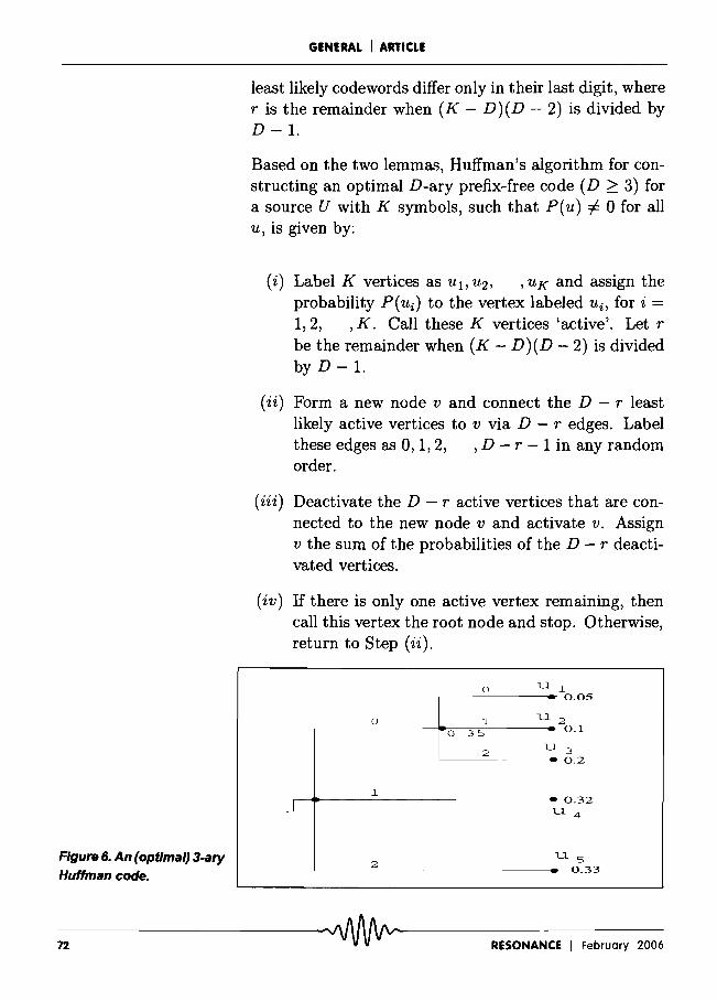
Figure 6. An (optimal) 3-ary

Huffman code.

GENERAL I ARTICLE

least likely codewords differ only in their last digit, where r is the remainder when (K - D)(D - 2) is divided by D-l.

Based on the two lemmas, Huffman's algorithm for con­structing an optimal D-ary prefix-free code (D 2:: 3) for a source U with K symbols, such that P( u) # 0 for all u, is given by:

(i) Label K vertices as Ul, U2, , UK and assign the probability P(Ui) to the vertex labeled Ui, for i == 1,2, ,K. Call these K vertices 'active'. Let r be the remainder when (K - D)(D - 2) is divided by D -1.

(ii) Form a new node v and connect the D - r least likely active vertices to v via D - r edges. Label these edges as 0, 1,2, , D - r -1 in any random order.

(iii) Deactivate the D - r active vertices that are con­nected to the new node v and activate v. Assign v the sum of the probabilities of the D - r deacti­vated vertices.

( i v) If there is only one active vertex remaining, then call this vertex the root node and stop. Otherwise, return to Step (ii).

o U l r--------____ 0.05

o l U 2 .------------=-0---=--3-=S------- 0.1

2 U 3

"------__e 0.2

l r---____ -------------- 0.32

2

U 4

Us 0.33

n --------------------------~-----------R-ES-O-N-A-N-C-E-I-F-e-br-u-ar-Y-2-0--06

GENERAL I ARTICLE

Example 6.3. Consider the same source U as in Example 6.1. The Huffman coding algorithm constructs a 3-ary prefix-free code as shown in Figure 6. The codewords corresponding to Ub U2, U3, U4, U5 are 00, 01,02, 1, 2, re­spectively. The average code-length is 2 0.05 + 2 0.1+ 2 0.2 + 1 0.32 + 1 0.33 = 1.35 ternary digits and the entropy of the source is H3(U) = 1.3038 ternary digits.

Remark 6.1. While the proof of Theorem 5.1 seems to suggest that the Shannon-Fano coding technique is a very natural technique to construct a prefix-free code, it turns out that this technique is not optimal. To il­lustrate the sub-optimality of this technique, consider a source with two symbols U1 and U2 with probabil­ity of occurrences p(ud = 1/16 and P(U2) = 15/16. The Shannon-Fano algorithm finds a binary prefix-free code with codeword lengths equal to fIog2 1A61 = 4

and fIog2 15/161 = 1, respectively, whereas the Huffman­coding algorithm yields a binary prefix-free code with codeword lengths equal to 1 for both.

7. Summary

This article has presented a derivation of the best achiev­able performance for a source encoder in terms of the average code length. The source-coding theorem for the case of prefix-free codes shows that the best cod­ing scheme for a source X has an expected code-length bounded between H (X) and H (X) + 1. Two coding techniques, the Shannon-Fano technique and the Huff­man technique, yield prefix-free codes which have ex­pected code-lengths at most one more than the source entropy. The Huffman coding technique yields an op­timal prefix-free code yielding a lower expected code­length compared to a corresponding Shannon-Fano code. However, the complete proof of the optimality of Huff­man coding [2] is not presented here; Lemma 6.1 only presents a necessary condition that an optimal code must satisfy.

Suggested Reading

[1] C EShannon,AMathemati­

cal Theory of Communica­

tions, BeU System Techni­

cal Journal, Vol. 27, pp.379-

423, july, 1948; Vo1.27, pp.

623 -6S6, October 1948.

[2] T M Cover and j A Tho­

mas, Elemenu of Informa­

tion Theory, Wiley Series in

Telecommunications,john

Wiley & Sons, Inc., New

York, 1991.

[3] j L Massey,AppliedDigi­

tal Information Theory 1.

Lecture Notes, ETH,

Zurich. Available online at

http://www.isi.ee.ethz.cb/

education/public/pdfs/

aditl.pdf

[4] R L Karandibr, On Ran­

domness and Probability:

How to Model Uncertain

Events Mathematically,

Resonance, Vol.l, No.2, Feb.

1996.

[5] W Feller,Anlmroduction to

Probability Theory and its Applications, Vols.l,2,

Wiley-Eastern, 1991.

[6] S Natara;an, Entropy, Cod­

ing and Data Compression,

ResOllllllCe, VoL6, No.9, 2001.

Address for Correspondence

Deepak Sridhara

Institut fUr Mathematik

Universitat ZOrich

Email:

sridhara@math.unizh.ch

-RE-S-O-N-A-N-C-E-I--Fe-b-rU-a-rY--2-00-6--------~~~-~--------------------------n-