GENERAL CHEMISTRY SECTION III: PHYSICAL STATES

LECTURE 14: STATES OF MATTER AND AN INTRODUCTION TO THE IDEAL GAS LAW

Chapter Summary

Talk about a change of pace. After half a semester on the theoretical underpinnings for the chemical bond, we get decidedly practical and consider the simple idea that matter can be fairly simply categorized by whether it’s a gas, liquid, or solid. The next several lectures will explore the theories that give rise to the empirical observations we can make about matter in its various states. The most interesting thing is that, when we explore condensed matter (liquids and solids), we will find that the concepts we developed in bonding can be applied to explain – and even predict – many of the properties that chemical compounds exhibit. First, we’ll consider gases. The simple models that explain most of gas behavior are actually founded on the idea that gas molecules are all the same, and, in fact, that everything we learned about the chemical bond is irrelevant to the study of gases. Yes, gases are both boring and easy.

This first lecture on gases is an elementary introduction, given in two parts: Part 1 – Nomenclature. A brief bit of history on the scientists who investigated gases, and then we’ll familiarize ourselves with some words used to discuss the nature of gases in a more sophisticated manner. Part 2 – Calculations.

Type 1 Static system PV = nRT Type 2 Change of state V1T1/V2T2

The second lecture develops somewhat more sophisticated ideas about gases.

Part 3 – Theory. We can use Kinetic Molecular Theory (KMT) to derive the ideal gas law (PV = nRT) and to calculate gas velocity, diffusion, and effusion. Part 4 – Ideal vs. non-ideal gases. We’ll see how PV = nRT works for “ideal” gases but, since gases are not actually ideal, the truth is that PV ≠ nRT in reality. Gases’ non-ideality is because of molecular attraction and size, both of which violate KMT.

156

156

Here’s a helpful hint that will come in handy from here on out in the course: we often discuss proportions/relationships between variables, and to do that we use the symbol α, which signifies a direct relationship between variables (when one increases or decreases, the other does the same). Its reciprocal (1/α or α-1) signifies an inverse relationship between variables (when one increases or decreases, the other does the opposite). For example, the more you watch or read the news, the more informed you are about the state of the world – directly proportional. But the more you watch or read the news, the less happy you are about the state of the world – inversely proportional. See? Easy.

USEFUL VARIABLES FOR GASES

In the lectures on thermodynamics we’ll have in a few weeks, we’ll learn a great deal about chemical systems: the environment in which our chemical species are found. They’re characterized by variables, like pressure or volume. Those variables are called state functions: properties for which we care only about the values before and after a reaction. We will learn how to quantify the relationship between these state functions using the ideal gas law:

P1, V1, T1, n1 It’ll often be the case that we will perturb our system with a reaction that changes the values of the state functions – giving us P2,V2,T2, n2 – and that the change in these state functions, represented as ∆P, ∆V, ∆T, ∆n, will be information that we want to know.

LET’S GET TO KNOW OUR STATE FUNCTIONS

n is the moles of a gas. The amount of gas is most easily defined by the mole and can be related through stoichiometry and other unit factors to other system parameters like: Note that the moles of gas are typically much smaller than other phases; gas density is much smaller than any of the others (about 1000 times less dense).

n = g/MW g = grams

MW = molecular weight

n = M•V M = molarity V = volume

ρ = g/V ρ = density g = grams

V = volume

157

157

V is the volume of the gas and has units like mL, L, gallons, ounces, etc. It’s defined by the space in which gases travel, which means it becomes very large in open environments. P is pressure, in units like atmospheres (atm). It tells the number of times gas molecules hit the surface of the container. T is the temperature of the system, and has units like K, °C, °F. It’s directly proportional to energy in the system.

KINETIC MOLECULAR THEORY (KMT)

Scientists sat around, thinking really hard about a model for gases. They decide the following is a good way to think of them, given that they seem to be rather boring chemically and have very low densities*:

• Gas molecules are hard spheres. • They are infinitely small in volume. • They have no attraction for either each other or the surface of system; therefore, collisions

are elastic (hitting another molecule or the container does not cause any loss of energy). • The energy in a gas system is constant and is determined by temperature.

• T α E ← (temperature is directly proportional to energy; if one increases or decreases, the other does the same). • The velocity of gas particles is determined by the equation:

E = ½ mv²

*These are “ideal” notions and are used to derive the ideal gas law.

Note that gas particles are all the same according to KMT, regardless of type. For example, He is an infinitely small particle that undergoes elastic collisions, and the same goes for CO2, N2, NH3, and H2O.

Important note about units of T: We most commonly use K (degrees Kelvin) and °C to measure T. You may not be familiar with K, and we’ll learn more about it

later, but for now, here’s a conversion you should know: °C + 273 = K

158

158

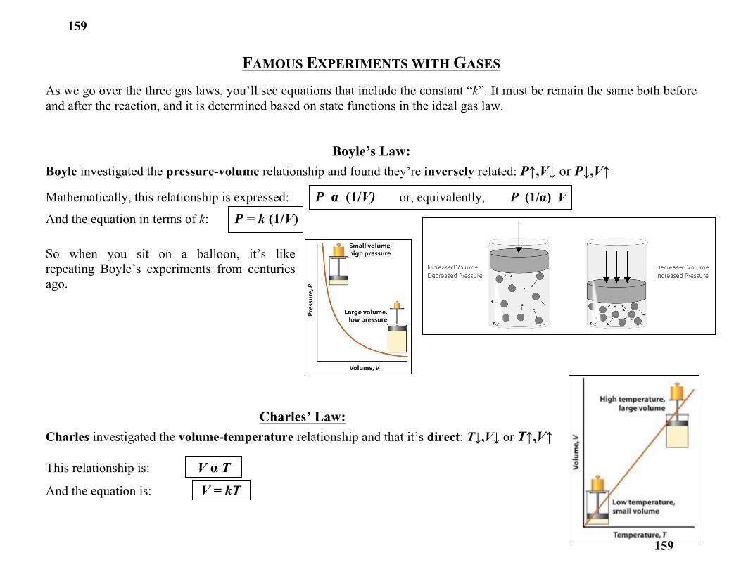
FAMOUS EXPERIMENTS WITH GASES As we go over the three gas laws, you’ll see equations that include the constant “k”. It must be remain the same both before and after the reaction, and it is determined based on state functions in the ideal gas law.

Boyle’s Law: Boyle investigated the pressure-volume relationship and found they’re inversely related: P↑,V↓ or P↓,V↑

Mathematically, this relationship is expressed: P α (1/V) or, equivalently, P (1/α) V

And the equation in terms of k: P = k (1/V) So when you sit on a balloon, it’s like repeating Boyle’s experiments from centuries ago.

Charles’ Law: Charles investigated the volume-temperature relationship and that it’s direct: T↓,V↓ or T↑,V↑ This relationship is: V α T

And the equation is: V = kT

159

159

Avogadro’s Law: Avogadro investigated the mole-volume relationship. He discovered the extraordinary idea that the more moles of gas you have, the bigger the balloon. In other words, n is directly proportional to V.

This relationship is: n α V

And the equation is: n = kV

COMBINING THREE LAWS GIVES US THE IDEAL GAS LAW Using a little algebra to combine these three relationships, and after consolidating the three constants into one, we have the ideal gas equation:

PV = nRT …where R is the ideal gas constant. Note the three experimental relationships are all present in this one equation. Also note this equation is true only under ideal conditions (KMT conditions). Let’s talk some more about R. It quantifies the properties of an ideal gas, which is really just a gas under standard conditions. We consider standard conditions – or, STP (for standard temperature and pressure) – to be:

T = 273 K = 0°C P = 1 atm = 760 torr = 101.3 kPa

Like all constants, R can be expressed in different ways depending on its units. While we learn about gases, our units are typically: atmospheres (atm) for P; liters (L) for V; and Kelvin (K) for T. With these, the appropriate value for R is:

R = 0.082 L•atm/mol•K

You should keep in mind, though, that R is also often used to relate energy (in Joules (J)) and T. In that case, it’s R = 8.314 J/mol•K. But we’ll focus on the former value for R during this unit on gases. So let’s see what kinds of problems can we work…

160

160

CALCULATIONS FOR A STATIC SYSTEM For static systems (systems that are not perturbed), we can perform simple calculations with the ideal gas law equation (P1V1=n1RT1). These are classic plug-and-chug calculations in which we are given three values to hold constant while we solve for a fourth, unknown variable. Example:

What is the volume of 1 mole of an ideal gas when it’s held at 1 atm and 273 K? Solution: Let’s first write down the variables we know (AKA “givens”):

P = 1 atm n = 1 mole T = 273 K R = 0.082 L•atm/K•mol

Now we need to rearrange it ideal gas law before we plug-and-chug: PV = nRT → V = nRT/P → [(1 mol) • (0.082 L•atm/K•mol) • (273 K)] / (1 atm) = 22.4 L

Look! All of the values we just used were those of the variables at STP! This means our answer tells us the neat fact that, at standard temperature and pressure, an ideal gas has a volume of 22.4 L. Here are two good things to think about while doing problems that don’t involve a change of state:

1. Remember how I said that there are many versions of R with different combinations of units? And that you should (for the most part) ignore those and just plan to use R = 0.082 L•atm/K•mol while we work with gases? Good, because those things are still true.

2. The trick to doing these problems is that you’ll often need to convert the values given to you for P, V, T, and n, into values that are consistent with R. That’s really the only complication for these questions. And usually the biggest hassle comes from getting a value that you need to convert into a number of moles…

161

161

How about we address that last sentence? It was kind of daunting, and with good reason – you’ll need to have a value for n in these calculations, but there are three “disguises” in which it can present itself to you: molecular weight (MW), density (ρ), and molarity (M). If you’re given information about one of these, you need to recognize it as a stepping stone to find n, because that’s your real variable of interest. Each of them can be converted into a number of moles through an equation: (Note: the “g” in these equations indicates a mass in units of grams.) These hopefully look a little familiar to you, because we learned them a few pages ago…

CALCULATIONS FOR A SYSTEM WITH A CHANGE OF STATE Anytime that a problem suggests that conditions in the system have been changed because of a perturbation, regardless of whether the change is happening to P, V, T, or n, you need to have an equation made from taking the ideal gas law, combining the two states you need, eliminating all other constants. We’ll go over a derivation of one of these so you appreciate the idea behind them. Say we have a system in which only the volume and temperature change over the course of the reaction: First off, since we know that only V and T changed, the other variables (n and P) must have stayed the same. So let’s rearrange the ideal gas law to have our changing-things on one side and our constant-things on the other: V/T = nR/P. Now, using our rearranged gas law, we’ll write out the equation for state #1 of the system (before reaction): V1/T1 = n1R/P1, as well as the one for state #2 (after reaction): V2/T2 = n2R/P2.

In our new equations, the terms the right side (nR/P) contain all the states that didn’t change, meaning their before-reaction and after-reaction values are identical. This means that n1R/P1 = n2R/P2. And if that’s the case, then we our state #1 and state #2 equations can be set equal to each other: V1/T1 = nR/P = V2/T2.

n = g/MW n = M•V

ρ = g/V

162

162

Ta-da! You’ve now derived the equation needed to solve an ideal gas law question that involves a change of state. The equation we just derived was for a change in V and T (left equation), but others can be created for systems with changes in P and V (middle equation), and systems with changes in – brace yourself – P, V, and T (right equation).

EXAMPLE CALCULATIONS: USING THE IDEAL GAS LAW

Example #1 – Simple ideal gas law: What is the pressure when 2.5 moles of H2 are placed in a 200 mL container at 50°C?

Solution:

First note that there is no change in state. We assume this is about ideal gases, so the equation is: PV = nRT. Our givens:

n = 2.5 moles V = 200 mL → Must convert this to L → V = 0.2 L T = 50°C → Must convert this to K → T = 50°C + 273 = 323 K R = 0.082 L•atm/mol•K

Now we solve (while being aware that units are canceling): P = [(2.5 mol) • (0.082 L•atm/mol•K) • (323 K)] / (0.2 L) = 331 atm ← That’s some pressure!

163

163

Example #2 – Ideal gas law, solving for MW: There are 0.87g of a gas put into a 5 L container at -50°C with a pressure of 76 torr. What is the MW of the gas?

Solution:

Derive an equation that includes our givens and MW: PV = nRT → PV = g/MW•(RT) → MW = g•RT/PV

Givens: g = 0.87g V = 5 L

P = 76 torr → Must convert this to atm → P = (76 torr) / (760 torr) = 0.1 atm T = -50°C → Must convert this to K → T = (-50°C) + 273 = 223 K Plug and chug: MW = [(0.87g) • (0.082 L•atm/mol•K) • (223K)] / [(0.1 atm) • (5 L)] ≈ 32 g/mol

Example #3 – Ideal gas law, solving for density:

What is the density of CH4 while at a pressure of 0.1 atm and a temperature of 414 K? Solution: Derive an equation that includes our givens and density (ρ):

PV= nRT → n = PV/RT → P•(g/ρ)/RT = (g/MW) → ρ/MW = P/RT → ρ = P•(MW)/RT Givens: P = 0.1 atm T = 414 K MW of CH4 = 16 g/mol ← Gotten from periodic table

Plug and chug: ρ = [(0.1 atm) • (16 g/mol)] / [(0.082 L•atm/mol•K) • (414 K)] = 0.047 g/L ← Not very dense.

164

164

Example #4 – Ideal gas law, using STP: What is the volume of C3H8 if 1 mole is kept at STP?

Solution: We know that STP is P = 1 atm, and T = 273 K. Plug and chug: V = [(1 mol) • (0.082 L•atm/mol•K) • (273 K)] / 1 atm = 22.4 L ← A famous volume, true for all gases. Example #5 – Ideal gas law, involving change of state in P and V:

Dr. Laude fills a balloon to a pressure of 1 atm and volume of 500 mL at 273 K. He then sits on it, changing the pressure to 5 atm. What is the new volume?

Solution: Identify which states are changing (P and V), and which are staying the same (n and T). Use that information to decide the correct equation to use for a change-of-state-problem: P1V1 = P2V2

Plug and chug: (1 atm)(500 mL) = (5 atm)(X mL) → (500 / X) = 5 → 100 mL ← Or 0.1 L; you’d check the answer choices.

Example #6 – Ideal gas law, involving change of state in V and T:

In a closed system at constant P and n, if the volume of the system is decreased by a factor of 10, the temperature: a) Goes up by a factor of 10. b) Goes down by a factor of 10. c) Remains constant. d) None of the above.

Solution: The answer is B.

V1/T1 = V2/T2 → so if V goes from 10 L to 1L, then T must decrease 10-fold to keep the proportions equal.

165

165

LECTURE 15: MORE ADVANCED IDEAS INVOLVING GASES

HOW FAST ARE GAS MOLECULES? From kinetic molecular theory (KMT) we know that:

T α E = ½ kT = ½ mv2

(Temperature term) (Velocity term)

Notice that the velocity can be easily determined from:

E = ½ mv² We can see from this that, the higher the temperature, the higher the velocity (direct relationship between v and T). Depending on mass and T, gas molecules move at hundreds of miles per hour, just at room temperature!

Note that the equation tells indicates an inverse square relationship between molecular speed and mass.

166

166

Example: At a certain temperature, H2 is traveling 1000 mph. How quickly is O2 moving at that temperature?

Solution: The E of the gas is the same regardless of T, so:

½ • mH2 • v2

H2 = ½ • mO2 • v2

O2 → 2 • v2H2 = 32 • v2

O2 → 32 / 2 = v2H2 / v

2O →

→ 16 = (1000 / v2O2) → √ everything → 4 = (1000 / vO2) → vO2 = 250 mph.

GAS MOVEMENT: DIFFUSION AND EFFUSION Despite that last answer, we know that gas molecules don’t really get around the room going hundreds of miles per hour. If they did, smells would come (and go) much faster than they do. The reason for their reduced speed is that (at atmospheric pressure) collisions constantly occur between molecules, which decreases their speed by many orders of magnitude. So what do they call this collisional velocity? Diffusion (show in the figure on the left). And a similar kind of velocity – called effusion (shown in the figure on the right) – has to do with the ability of gas molecules to get through a pin hole.

In both cases, the rate of effusion and diffusion is the same inverse square relationship as speed. So, if we know O2 has a velocity that is 4-fold slower than that of H2, we also immediately know that its diffusion and effusion is also 4-fold slower.

167

167

NON-IDEALITY OF GASES Is KMT flawed? Recall that when we were first introduced to gases, we learned that, according to KMT:

• Gas molecules have no volume (we called them infinitely small). • Gas molecules are not attracted to each other, so all collisions are elastic.

But in reality, neither of those statements is completely true…

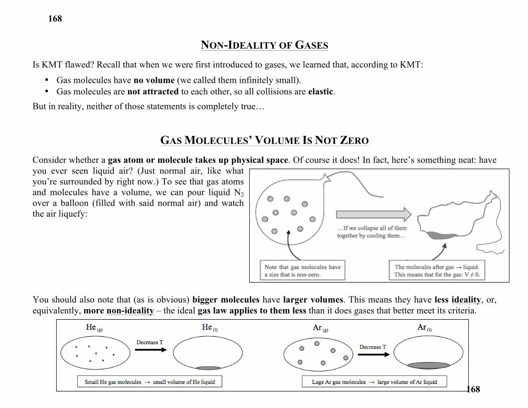
GAS MOLECULES’ VOLUME IS NOT ZERO Consider whether a gas atom or molecule takes up physical space. Of course it does! In fact, here’s something neat: have you ever seen liquid air? (Just normal air, like what you’re surrounded by right now.) To see that gas atoms and molecules have a volume, we can pour liquid N2 over a balloon (filled with said normal air) and watch the air liquefy: You should also note that (as is obvious) bigger molecules have larger volumes. This means they have less ideality, or, equivalently, more non-ideality – the ideal gas law applies to them less than it does gases that better meet its criteria.

168

168

ATTRACTION BETWEEN GASES Gases bump into each other and will momentarily “stick” together. So their collisions are actually somewhat inelastic – not by much (or they wouldn’t be gases), but still by an amount worth mentioning. And the bigger the molecule, the more polar – and “sticky” – it is. Why does this matter? – Because if at any given time some particles are stuck together, the number of particles hitting the sides of the container decreases, which means that P↓.

CORRECTING FOR NON-IDEALITY How do we correct for gases that are not ideal? – By using fudge factors that are specific to each gas and account for its non-ideality; so if PV ≠ nRT, then we use:

(P + “fudge factor”) • (V + “fudge factor”) = nRT …Where P’s fudge factor accounts for the attractive forces the gas law ignores, and V’s accounts for molecules’ volume. Non-ideal gas laws incorporate these fudge factors; one such law is the van der Waals equation:

(P + n²a / v² )(v - nb) = nRT Here, a and b are fudge factors that are specific to the kind of gas. The bigger any gas’ a and b, the more non-ideal it is – so there’s a direct relationship between the magnitude of the fudge factors, and the non-ideality of the gas. For example, consider the following:

Helium → a = .0034 and b = 0.237 NH3 → a = 4.17 and b = 3.71

This means helium is small and not attracted (or attractive) to NH3, while NH3 is bigger and very attracted to most gases.

169

169

WHEN IS A GAS MORE IDEAL? Gases behave more ideally when fewer collisions are taking place between molecules, which happens at high temperature and low pressure. Specifically regarding small, non-polar gases: since both their volume and attractive forces are small, they behave more ideally than larger and/or polar gases.

SUMMARIZING TRENDS BASED ON SIZE

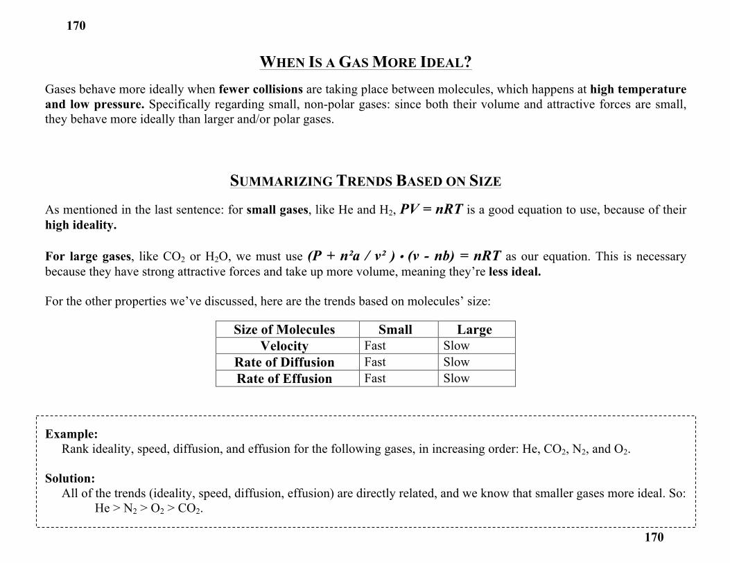
As mentioned in the last sentence: for small gases, like He and H2, PV = nRT is a good equation to use, because of their high ideality. For large gases, like CO2 or H2O, we must use (P + n²a / v² ) • (v - nb) = nRT as our equation. This is necessary because they have strong attractive forces and take up more volume, meaning they’re less ideal. For the other properties we’ve discussed, here are the trends based on molecules’ size:

Size of Molecules Small Large Velocity Fast Slow

Rate of Diffusion Fast Slow Rate of Effusion Fast Slow

Example:

Rank ideality, speed, diffusion, and effusion for the following gases, in increasing order: He, CO2, N2, and O2.

Solution: All of the trends (ideality, speed, diffusion, effusion) are directly related, and we know that smaller gases more ideal. So:

He > N2 > O2 > CO2.

170

170

Example: At a certain temperature, helium travels with a velocity of 300 mph. What is the MW of a gas that, at the same temperature, has a velocity of 150 mph?

Solution:

First off, we know that, at the same temperature, the E of the system is constant, so we don’t have to worry about T. We also know that the equation relating V and E for all gases is: Esys = ½mv². So for our two gases:

EHe = ½m1v1² and, Eother gas = ½m2v2² Now let’s rearrange them to put our variable of interest (m2) on one side of the equation:

m2 = m1v1²/v22

Plug and chug: m2 = (4 g/mol)(300 mph / 150 mph)² = 16 g/mol

Example – Ranking ideality (which also means velocity): Rank the following gases in terms of increasing non-ideality: He, O2, N2, and CH4.

a) He < N2 < O2 < CH4. b) He < CH4 < N2 < O2. c) O2 < N2 < CH4 < He. d) CH4 < O2 < N2 < He.

Solution:

The answer is B. In general, the bigger and slower the gas molecule, the less ideal. Among these gases, O2 is biggest and He smallest;

therefore He is most ideal, and O2 least ideal. In class we’ll assume that size is proportional to molecular weight. A word of caution about ranking problems: Make sure you pay attention to the rank you’re asked for, and that you’re actually ordering it correctly; that might sound stupidly obvious, but backwards-ranking is a common mistake. In the last example, we were asked for “increasing non-ideality”; you obviously know what this means, but make sure you think about it – the least non-ideal (or, equivalently, the most ideal) should be listed first, and the most non-ideal (or, equivalently, the least ideal) should be last. Be careful that you don’t think of it backwards, because that will always be an answer choice.

171

171

LECTURE 16: INTRODUCTION TO INTERMOLECULAR FORCES (IMF’S) As we ended the lectures on gases, we were introduced to an idea that serves as foundation for the material in this lecture: kinetic molecular theory says that colliding gas molecules exhibit that no attractive forces to each other – but that’s not actually the case. We learned that non-ideality arises because of the attractive forces between colliding molecules, and that consequently, PV ≠ nRT. So can we explain the source of this non-ideality? It is important because this non-ideality from attractive collisions explains how liquids and solids form.

…And we see that as T increases, P decreases – they are inversely proportional. So the lectures on liquids and solids must begin with a better understanding of intermolecular attraction. Let’s get started by looking at attractive forces more generally:

172

172

Two examples of Coulombic attraction can be distinguished in matter:

Intramolecular forces are bonds inside molecules (holding them together); these are either ionic or covalent. Intermolecular forces (IMF’s) are attractions between molecules; they exist outside the molecules.

INTERMOLECULAR BOND STRENGTHS So now let’s get quantitative with bonding. Notice that intramolecular bonds are 1 to 2 orders of magnitude stronger than intermolecular forces. (Even still, it is the weak intermolecular forces that allow liquids and solids to form.) Here are some facts about IMF’s:

• They are responsible for solution properties like boiling point and viscosity.

• Their relative magnitude is determined from the existence of dipoles in molecules (which comes from ΔEN).

• You can rank solution properties based on ΔEN calculations.

173

173

An interesting side note about ionic bonds: they are both inter- and intramolecular. Why?

Now on to the rest of the lecture. What are the solution properties we’re interested in? (You need only to know their definitions and a brief theoretical explanation about their relationship to intermolecular forces.)

BOILING POINT This is a process that happens when an increase in temperature causes a system’s energy to increase, thus breaking IMF’s and resulting in a vaporized (gas) molecule. However, for a molecule to escape liquid, enough gas molecules need to be made in order to raise the vapor pressure above atmospheric pressure. This is the definition of boiling. The boiling point reflects the energy needed to induce boiling.

Relationship to IMF’s – directly proportional.

The bonds in a crystal are not as distinct as they are in a molecule. Hence the ambiguity in inter- and intramolecular bonds. Look at the salt crystal on the left. Notice that there is no single Na—Cl unit anywhere. Instead, each Na+ has ionic bonds to all 6 of the Cl- molecules around it (or <6 if the Na+ is on the side of the crystal); the same goes for each Cl-.

174

174

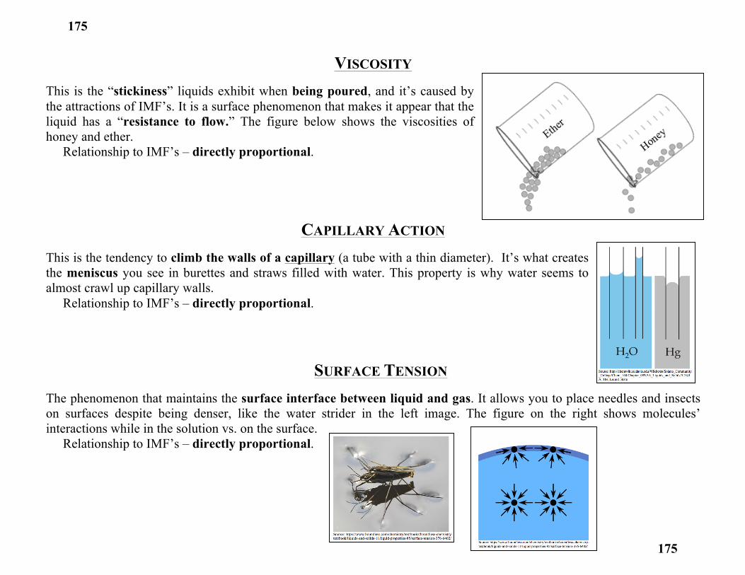
VISCOSITY This is the “stickiness” liquids exhibit when being poured, and it’s caused by the attractions of IMF’s. It is a surface phenomenon that makes it appear that the liquid has a “resistance to flow.” The figure below shows the viscosities of honey and ether.

Relationship to IMF’s – directly proportional.

CAPILLARY ACTION This is the tendency to climb the walls of a capillary (a tube with a thin diameter). It’s what creates the meniscus you see in burettes and straws filled with water. This property is why water seems to almost crawl up capillary walls.

Relationship to IMF’s – directly proportional.

SURFACE TENSION

The phenomenon that maintains the surface interface between liquid and gas. It allows you to place needles and insects on surfaces despite being denser, like the water strider in the left image. The figure on the right shows molecules’ interactions while in the solution vs. on the surface.

Relationship to IMF’s – directly proportional.

175

175

EVAPORATION This is a surface phenomenon that explains why solution molecules enter gas phase. This is different from boiling in that it occurs at surface, but it is also temperature dependent.

Relationship to IMF’s – inversely proportional (in reference to the evaporation rate).

ΔHVAP

Technically called the “enthalpy of vaporization,” this is a thermodynamic term that tells you the amount of energy required for a liquid to become a gas. It is found in boiling and evaporation equations.

Relationship to IMF’s – directly proportional.

VAPOR PRESSURE This is the flip side of evaporation – it is the pressure pushing down on liquid by its already-evaporated molecules. Obviously, if ΔHvap is small, vapor pressure is large – there is an inverse relationship between ΔHvap and vapor pressure.

Relationship to IMF’s – inversely proportional.

176

176

RANKING SOLUTION PROPERTIES: OUR PREDICTIONS Now that we have seen the various solution properties and how they relate to IMF’s, let’s see whether we can predict the ranking of various molecules for a solution property. Can I rank the solution properties of compounds? Yes, and it’s easy. For example, I can rank H2O, CH3Cl, and N2 in order of increasing ΔHvap in less than ten seconds. The answer is: N2 < CH3Cl < H2O. …How’d I do that?

ELECTRONEGATIVITY: AN OLD FRIEND In a nutshell, you can relate the three kinds of intermolecular forces directly to the magnitude of solutions’ properties:

Summary of relationships to IMF’s:

IMF’s are directly proportional to: boiling point, viscosity, capillary action, surface tension, and ΔHvap. As IMF magnitude increases, so do the magnitudes of the above properties.

IMF’s are inversely proportional to: evaporation and vapor pressure. As IMF magnitudes increase, the magnitudes of the above properties decrease.

To figure out the magnitude of IMF’s, you need to be able to create 3D Lewis structures for molecules, assign atoms’ EN’s, identify all dipoles, cancel them out if possible), and determine whether a net dipole exists. (You did all of this in unit #2, when we learned how to draw the 3D structures of molecules.)

177

177

Example, part #1: Predict the ranking of solution properties for N2, CH3Cl, and H2O.

Solution:

The steps to take: 1. Create the 3D Lewis structures. 2. Assign EN to each atom. 3. Identify all dipoles. 4. Determine whether a net dipole is present (Σ ΔEN ≠ 0).

When you do these, you find: N2 → no net dipole → nonpolar. CH3Cl → has a net dipole → polar. H2O → has a net dipole → polar.

Example, part #2:

What does the above information tell us about the solution properties of these molecules?

Solution: N2 → Since it’s nonpolar → it only forms instantaneous dipoles. CH3Cl → Since it has a net dipole → strongest IMF is dipole-dipole; instantaneous dipoles are also present. H2O → Since it has a net dipole → forms dipole-dipole; BUT it has an H bonded to an EN atom → also H-bonding, which is its strongest IMF. (Also has instantaneous dipoles.)

So in terms of solutions properties, we can say generally that:

For properties directly proportional to IMF strength → N2 < CH3Cl < H2O. For properties inversely proportional to IMF strength → H2O < CH3 < N2. Notice that the ranking is the same for properties that are directly vs. inversely proportional, except that their orders are reversed.

Get really good at creating 3D structures and assigning polarity – it is the essential step in explaining IMF’s in solutions.

178

178

LECTURE 17: THEORY BEHIND INTERMOLECULAR FORCES Intermolecular forces (IMF’s) are forces of attraction between individual molecules. As we have just seen, there exists a direct correlation between the strength of IMF’s in a solution and the magnitude of its properties (e.g., viscosity, boiling point, ΔHvap, evaporation).

Type of IMF Strength (kJ/mol) Instantaneous Dipole <1

Permanent Dipole 1-5 Hydrogen Bonding 10-20

Let’s look more deeply at reasons for the magnitude of each of these kinds of intermolecular forces.

PERMANENT DIPOLES Permanent dipoles occur in molecules that are not completely symmetrical, which, as we learned in previous lectures, are also molecules with a total electronegativity that does not equal zero (∑ΔEN ≠ 0). (Recall: “total/overall electronegativity” is the electronegativity values of all the species are added together.) CF4 does not have a permanent dipole → it is symmetrical (and ∑ΔEN = 0). CCl3H does have a permanent dipole → it is not symmetrical (and ∑ΔEN ≠ 0).

179

179

Permanent dipoles are one type of IMF’s. Each molecule possesses an area of δ- with a relatively high electron density (“partial positive charge”), as well as an area of δ+ with a relatively low electron density (“partial negative charge”). As dipoles of nearby molecules align, attractions are created (figure below); to the left is a figure of NH3’s dipoles.

INSTANTANEOUS DIPOLES Unlike asymmetrical molecules, symmetrical molecules have weak IMF’s! This is why N2 or He can be liquid at room temperature. But why do symmetrical molecules – with ∑ΔEN = 0 and no permanent partial charges – have any attraction at all? Because of instantaneous dipoles. So what are these instantaneous dipoles? Well, although it’s true that symmetrical molecules have ∑ΔEN = 0 over time, they will actually have moments where – for an instant – a dipole will exist in the molecules, and a weak attraction forms. These occur because electrons are constantly whizzing around, so even though a molecule might not have any atoms that are more electronegative than others, the electrons may just happen to be briefly near each other; for that tiny instant, the e--density is, in fact, higher on one side of the molecule, and it therefore has a partial charge. If this happens to adjacent molecules, their momentary partial charges can experience a short-lived attraction. Important facts about instantaneous dipoles:

1) They are also known as London forces, dispersion forces, or Van der Waals forces. 2) They are the reason that noble gases can form liquids and solids. 3) Alone, they are mostly insignificant; but as molecules increase in magnitude, dispersive forces can integrate and add

up to be something quite substantial, kind of like Velcro.

(δ+) • • • • (δ–) • • • • (δ+) • • • • (δ–) • • • • (δ+) • • • • (δ–)

180

180

HYDROGEN BONDS: A PERMANENT DIPOLE SPECIAL CASE Hydrogen bonds (H-bonds) are the strongest IMF’s, and they’re the rationale behind the phenomenon of H2O – a molecule with a molecular weight of 18 g/mol that doesn’t boil until 100°C. The permanent dipoles we just learned about are indeed found in water, but they’re exceptional in its case – the bond contains an extremely electropositive hydrogen:

The atom bonded to hydrogen pulls the electron density away from it, which results in a small, densely, positively-charged region on the molecule. This is a prime δ+ for other molecules to be attracted to (via their δ- regions). H-bonding is especially strong in atoms of the second row because of the high electronegativity values of nitrogen, oxygen, and fluorine. Those elements with high EN have a strong pull on their bonded electrons, which results in regions of δ+ and δ- on the molecule. With these things in mind, our definition for a hydrogen bond should make sense:

• A hydrogen must be one of the atoms of the bond. • The hydrogen must be attached to an highly EN atom, such as N, O, F, or Cl.

Instantaneous dipoles are the reason some hydrocarbons (molecules

consisting only of H and C) are liquids at room temperature – the more C’s and H’s in the hydrocarbon, the more

opportunities for instantaneous dipoles; more instantaneous dipoles makes a compound harder to change from solid → liquid → gas. Hence, longer hydrocarbons have higher

boiling points.

181

181

This means that H2O, HF, HCl, and NH3 all exhibit H-bonding. On the other hand, CH3Cl does not because chlorine is not the atom bonded to the hydrogen in the molecule:

A more general definition is that H-bonding occurs for any hydrogen bonded to another atom. Thus, H2S, H2Te, and PH3 all have hydrogen bonding, though it is very weak: A final example – let’s compare IMF’s and solution properties in propane (C3H8) vs. water:

Solution Propane Water Polarity Nonpolar Polar

Strongest IMF Instantaneous dipoles Hydrogen bonding Boiling point -42°C 100°C

Vapor pressure 4500 torr 18 torr ΔHvaporization 16 kJ/mol 41 kJ/mol

Hydrogen bonding is possible.

Hydrogen bonding is not possible.

Since H2O has H-bonding, its: 1. Boiling point is larger. 2. Vapor pressure is lower. 3. ΔHvap is higher.

182

182

LECTURE 18: SOLIDS As you remove energy from a system, IMF attractions increase. Once enough energy is lost, gases turn into liquids, and liquids turn into solids.

Gases → Liquids → Solids

Decreasing Energy

Not all solids are ordered (e.g., plastic), but under certain circumstances, crystalline solids can form with specific geometrics. There are seven types of primitive geometric cells (three-dimensional), called unit cells: one is cubic, comprised entirely of right angles and sides of equal length; the other six are slightly less simple, as they vary in angle measure and side lengths. These unit cells can be merged by overlapping them to form more complex structures – crystals.

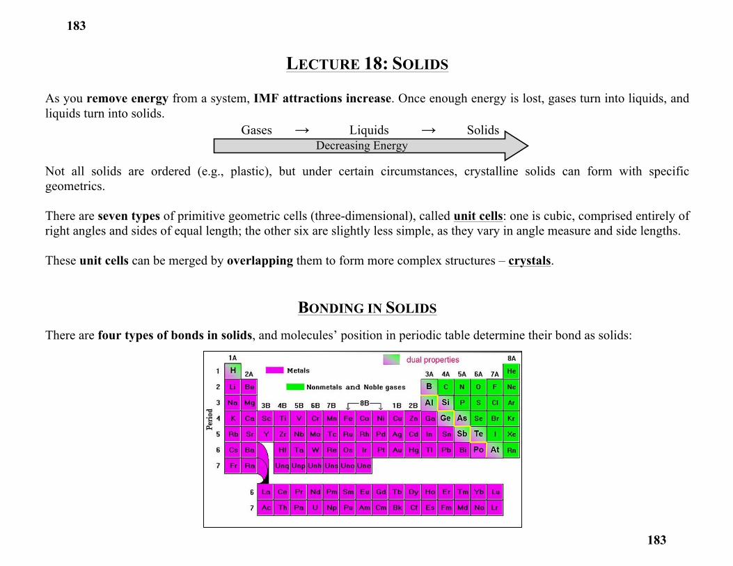
BONDING IN SOLIDS There are four types of bonds in solids, and molecules’ position in periodic table determine their bond as solids:

183

183

As you can see from the periodic table on the previous page, the majority of elements form metallic bonds when in solid form. However, the nonmetals and noble gases on the right form the other three types of bonds:

1) Metallic bond: a metal bonding with another metal; these are very strong bonds. Examples:

… –Cr–V–Cr–V– … … –Al–Al–Al–Al– …

2) Ionic bond: a metal bonding with a nonmetal; these have ~200 kJ/mol. Example:

… –Na–Cl–Na–Cl– …

3) Covalent bond: a nonmetal bonding with another nonmetal; these have ~400 kJ/mol. Examples:

Graphite → … –C–C–C–C– … Glass → … –Si-O-Si-O– …

4) IMF’s between molecules: solids can also be formed from H-bonds, dipoles, and/or dispersion; these are the weakest solids at ~1-20 kJ/mol.

Example: … –H–O–H • • • • • O–H– …

184

184