General Information Manual

IMPACT - Inventory Management Program

And Control Techniques

General Information Manual

IMPACT - Inventory Management Program

And Control Techniques

@ 1962 by International Business Machines Corporation

Copies of this and other IBM pUblications can be obtained through IBM Branch

Offices. Address comments concerning the contents of this publication to

IBM Technical Publications Department, 112 East Post Road, White Plains, New York

CONTENTS

Chapter 1: Overview . . . . . . . . . . . . . · 1 Development of Management Science. . · . . 1 Impact of Management Science. . . . . . . . . . The Role of Electronic Data Processing .

· 1 · • • 2

The Inventory Problem . . . . A Typical System. . . . . Guide to Reading This Manual

Chapter 2: Inventory Characteristics A Guide to Item Classification. .

• 2 · . • • • 3

• • • 3

· 4 · 4

Estimating Effects of Management Decisions . . . . . 6 The Standard Ratio . . . . . . . • 6 Other Listings by Value 8

Chapter 3: Order Quantity . . . . • . . . . . . . . . . 9 Least-Cost Strategies: The Trial-and-Error Approach . • • 9 Least-Cost Strategies: Solution by Formula . . . . . 10 Cost Elements of Lot-Size Formula. . . . . . . . . . . 11 Maintenance Costs . . . . . . Cost of Purchasing . . . . . . Derivation of Lot-Size Formula . . . . Quantity Discounts . . . . Joint Replenishment . . . •

Chapter 4: Order Point Lead Time .... Review Time Forecast of Usage per Time Unit. . Measure of Forecast Error . . .

Chapter 5: Service and Safety Stocks . . . . Playing the Odds . . . . . . . . . . . . • Safety Stock Based on Deviation . . . . Calculating the Standard Deviation . . . . • . An Approximation of Standard Deviation . Ways of Measuring Service . ..... . Summary. . . .. . .... .

Chapter 6: Forecasting . . . . . . . Common Forecasting Schemes. . . . . A Newer Scheme: Exponential Smoothing Controls . . . . . . . . Trend and Double Smoothing. . . . . . . • . Seasonal Forecasting Special Forecasting Problems .

Chapter 7: System Implementation . Study Organization System Characteristics System Development. . . . . • . System Planning . System Initializing System Operation. . . . . Pre-Study Activity . . . .

· . . . .12 · . . . .12

· .13 · .13

· .• 15

· .21 .21

• • • • .22 · • .22 · .. 22

· •• 24 .24

· .25 • .26 · .26 · .27 • • 28

• .29 · .31 · .32 • .36 · .37 · .39 · .39

· .41 · .41 · .41

.41

• .42 · .42 · .43

. . . • .43 Implementation Schedule . . . . . . . . ~ .44 Summary .....••. .44

CHAPTER 1: OVERVIEW

During the past decade, business and trade publica­tions have been increasingly filled with articles on scientific management. Many large corporations have added operations research or management science sections to their staffs, and graduate schools of business have added whole new departments in these subjects. Consulting firms specializing in management science have multiplied and prospered. Bookstores have had to add whole new sections to house the many books published in this field.

One area to which the new group has turned its attention is the management of inventories - in many cases with spectacular results. Improved customer service and reductions of up to 50% in inventories have been widely reported. One consulting firm has worked with 100 companies to reduce aggregate in­ventory by about $500, 000, 000. Lowering inventory investment has universal appeal, but of perhaps greater significance is the positive control placed in the hands of management. For the first time, eval­uation of the probable consequences of decisions is possible before the decisions are implemented.

IBM has investigated these new methods and has developed a standardized approach termed "IMPACT" - Inventory Management Program And Control Technique. To assist distribution industries in implementing positive control over when and how much to buy, an IMPACT Computer Program Library has been developed. This manual presents the principles of IMPACT in layman's language.

Development of Management Science

During World War II several small groups of scien­tists turned their attention from their normal interests to such problems as hunting submarines and establishing bombing patterns, with remarkable results. After the war some of them applied the same scientific approach to the solution of business problems and again had notable success.

The steps which characterize this method of seeking improved business decisions are:

1. Analyze the operation and identify the important and relevant factors which should influence decisions.

2. Express these factors in a quantitative way. 3. Determine the optimum way in which these

factors should be considered. 4. Test that the consequences implied by the

analysis are borne out in the real situation. Some­times the first trial shows the need to return to step 1 to gain a better understanding.

5. When a satisfactory solution is demonstrated, implement the results.

6. Incorporate controls to provide management with the information it needs to manage effectively.

Impact of Management Science

Management today is often in the frustrating position of establishing policy which is never carried out explicitly. This condition results sometimes from poor communications, and sometimes from the fact that people at the operating level lack the skills which managers could bring to bear if they had the time. It is by no means uncommon to discover two different policies regarding inventory in the same company; one is management's policy, and the other is the stock clerk's interpretation of management's policy. If a good manager had the time to control stocks, he would at least have some feel for what he meant in saying "keep inventory as low as possible consistent with good customer service". Unfortu­nately, the stock clerk is not clear on how low "low" is, or how good "good" is. Some managements try to help by being a little more specific, giving guides to the dollar level and service percentage desired. These guides at least give the stock clerk an indica­tion of when he is wrong, but his technique for trying to be right is trial-and-error, an expensive and often incorrect way.

Executives have been dissatisfied with the opera­tion of such systems. They have tried to make certain that policy is implemented by making the decision process a matter of routine. This has taken the form of directives such as, "When available stock gets down to three weeks' average usage, order enough to bring it up to six weeks." The standard for judging the performance of this system is that inventory level and service level seem "right"; no analysis is made to ascertain whether two weeks and five weeks might be better. If manage­ment wanted to improve customer service, they might change the rule to read, "When available stock gets down to four weeks' average usage, order enough to bring it up to six weeks." It is impossible to pre­dict the effect except to say that service would probably be "better" and inventory would be "higher". The extent of the change can be measured only by experience some weeks or months after the new rules have been adopted.

Management science brings extremely powerful controls to the management of inventories. For the first time, it becomes possible to (1) assess the probable consequences of policy decisions before they are implemented, and (2) having implemented these decisions, have confidence that they will in fact be carried out. Statistical theory can give answers to such questions as:

• What level of service can be provided with $3, 000, 000 of inventory? What will the associated costs of purchasing be?

1

• What level of inventory is required to provide 98% service? How much more would it take to provide 99% service?

• If $500, 000 is removed from inventory, how long will it take, and what effect might it have on the purchasing/receiving section?

The Role of Electronic Data Processing

Recently, computer technology has advanced to the point where electronic data processing is within the reach of many businesses which have previously been limited to unit record machines. A notable feature of computers has been the greatly increased speeds of card reading and printing. As often as not, the computer has been appealing solely because of these higher input/output speeds. Certainly the faster production of present jobs can justify a computer, but this does not take advantage of its full potential. Such use of a computer is rather like eating only the frost­ing on a cake.

The computer's special advantage lies in its ex­tremely powerful logical and mathematical abilities. By putting these special abilities to effective use, tremendous additional profit may be realized. Com­plex calculations and data manipulations which were hitherto impractical can now be made routinely. It is now relatively easy to get new kinds of information, rather than just the same kind faster.

An inventory management system is one of the most profitable ways to combine the computer's power and the tools of management science. Such a combination c an give management an entirely new and powerful arm in implementing its objectives effectively.

The Inventory Problem

To management, inventory is an aggregate or total mass of goods. Inventory serves the function of making a company's internal operation relatively stable, while providing service to customers. It is possible to reduce inventory by purchasing more fre­quently, in smaller lots. However, the processing of many small orders to the distributor's vendors and the increased receiving load would be likely to result in serious disruption of operations. Further, a sub­stantially smaller inventory might incur risk of unacceptable delays in filling customer orders.

On the other hand, if inventory were substantially larger, the operation would be much smoother, but the capital investment might be intolerable. Manage­ment attempts, therefore, to strike some middle ground where an acceptable inventory investment buys an acceptable degree of smoothnes s in internal operations.

2

While management may think of inventory as one large mass, the size of that mass is determined by tens (or even hundreds) of thousands of decisions relating to individual items during the course of a year. Policy directives, no matter how specific, must ultimately be reduced to the ordering strategy for a single item.

There are really only two fundamental questions facing anyone with responsibility for replenishment of an item's inventory. Implicit in both questions is the need to balance conflicting cost factors in order to minimize the total cost.

The first question is, "When do we order - in other words, how low should we allow our stock to get before we order?" This has traditionally been called the order-point question, a useful term to remember. For distribution industries, the concepts of inventory management have their greatest impact in setting order point. It is unlike a "minimum" in the usual sense, because it is not fixed but variable, in order to adjust to changing conditions. In answering this question at least two opposing costs must be con­sidered: the cost of lost sales or extra work caused by stockouts and the cost of carrying more inventory than is needed to meet demand. A decrease in one cost can be realized only by an increase in the other. The buyer must say to himself, "Should we order now, or wait?" or, in quantitative terms, "We now have 110 in stock. Do we need to order now, or can we wait until we get down to 90?" He is, then, determining a point in time (which is usually expressed as a quantity) beyond which he runs a risk of being out.

If he decides that it is time to order, he faces the second fundamental question: "How much should we order - in other words, should we order enough for a week, a month or a year?" Once again at least two opposing costs ought to be balanced and minimized: the operating costs of bringing an item into inventory, and the cost of maintaining an item in inventory . Clearly, as one goes up, the other goes down. The buyer is seeking to set order quantity, another useful term to remember.

It is quite likely that structuring the inventory problem in this way is a different approach for some readers, many of whom use the "fixed interval" system whereby a variable quantity is ordered at fixed period­ic intervals. Equally adaptable to inventory manage­ment techniques, the fixed-interval system is discussed under "Joint Replenishment", page 15. In introducing the basic concepts, however, we shall limit our dis­cussion to the "order point, order quantity" system to avoid confusion.

The bulk of this manual deals with new ways of answering the two basic questions, and we cannot suggest too strongly that you have them clearly differentiated before you go beyond this overview.

A Typical System

It may be helpful, before getting involved in the separate parts of an inventory management system, to have a general idea of how the parts might work together in a typical system. The reader should not expect to fully understand the relationships and fre­quencies just yet, but will find it easier to gain perspective by seeing the final framework now and referring back to it from time to time.

The total system is made up of three basic sub­systems: ordering, forecasting and reviewing. Balancing the costs of operating each subsystem against the sensitivity of the expected results leads us to specify a different frequency of use for each subsystem.

The ordering subsystem considers the order quantity, or how much to order, balancing the cost factors relevant to ordering strategy to find the minimum-cost strategy for each item. As we shall see in the section entitled "Order Quantity", it is usually not worthwhile to recalculate order quan­tities more than once or twice a year. The pertinent cost factors are the cost of purchasing, the cost of maintaining inventory, the effective unit cost, and the sales rate.

The forecasting subsystem has to do with the order point, or when to order. To know when to order, we must have some idea of how fast an item is going to be used up, so we forecast each item's usage rate. In order to recognize changes in usage patterns, we forecast relatively frequently, a monthly or semimonthly interval being most common. These forecasts are used to set order points, taking the cost of lost sales and the cost of maintaining inventory into account.

The reviewing subsystem is the least complex mathematically, closely paralleling the action of a buyer as he reviews either ledger cards or a stock status report. The order point set by the forecasting subsystem is compared with the available stock to determine whether stock is sufficiently low to order now. If it is not, no further action is indicated. If it is, the reviewing subsystem looks up the order quantity computed by the ordering subsystem. This quantity is then sent to the buyer for his approval. Reviewing should be done frequently because of the constant depletion of stock and the attendant possi­bility of reaching order point. It is not uncomcmon to check an item's status after every issue, though weekly and biweekly review are often encountered as well.

A general picture of how the subsystems fit together is given in Figure 1. The time intervals shown are merely representative and need not be restrictive.

Compute New

Forecast

Set Order Point

FORECASTING

SUBSYSTEM (Monthly)

REVIEW

SUBSYSTEM

(After each issue)

Notify Buyer

Is Now Time

To Order?

How Much?

Get Previously

Computed Order Qty

Compute Order

Quantities To

Minimize Total Cost

ORDERING SUBSYSTEM

( Semiannually)

Figure 1. A representative inventory management system

Guide to Reading This Manual

An attempt has been made to organize this manual for maximum ease of understanding, and we urge the reader to proceed sequentially. On the other hand, a good teaching organization is not always best for subsequent use as a reference manual. According­ly, some sections contain material which fits there logically, but which is nonessential to an initial understanding of basic concepts. A conspicuous example is the inclusion of quantity discounts and joint replenishment in the section on order quantity. We recommend bypassing these subjects on a first reading. The sections on safety stock and forecasting become more and more detailed as they progress, and the executive may wish to stop short of the end of these sections. One word of caution is in order: while top management need not be familiar with minute details, they should have a sufficient under­standing to use scientific inyentory management effectively, and someone in the organization must be completely familiar with every aspect of this powerful new tool.

3

CHAPTER 2: INVENTORY CHARACTERISTICS

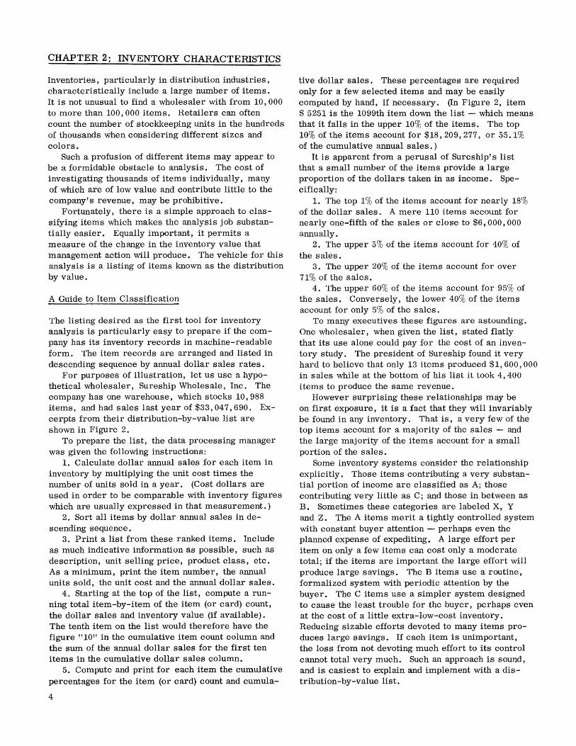
Inventories, particularly in distribution industries, characteristically include a large number of items. It is not unusual to find a wholesaler with from 10,000 to more than 100,000 items. Retailers can often count the number of stockkeeping units in the hundreds of thousands when considering different sizes and colors.

Such a profusion of different items may appear to be a formidable obstacle to analysis. The cost of investigating thousands of items individually, many of which are of low value and contribute little to the company's revenue, may be prohibitive.

Fortunately, there is a simple approach to clas­sifying items which makes the analysis job substan­tially easier. Equally important, it permits a measure of the change in the inventory value that management action will produce. The vehicle for this analysis is a listing of items known as the distribution by value.

A Guide to Item Classification

The listing desired as the first tool for inventory analysis is particularly easy to prepare if the com­pany has its inventory records in machine-readable form. The item records are arranged and listed in descending sequence by annual dollar sales rates.

For purposes of illustration, let us use a hypo­thetical wholesaler, Sureship Wholesale, Inc. The company has one warehouse, which stocks 10,988 items, and had sales last year of $33,047,690. Ex­cerpts from their distribution-by-value list are shown in Figure 2.

To prepare the list, the data processing manager was given the following instructions:

1. Calculate dollar annual sales for each item in inventory by multiplying the unit cost times the number of units sold in a year. (Cost dollars are used in order to be comparable with inventory figures which are usually expressed in that measurement.)

2. Sort all items by dollar annual sales in de­scending sequence.

3. Print a list from these ranked items. Include as much indicative information as possible, such as description, unit selling price, product class, etc. As a minimum, print the item number, the annual units sold, the unit cost and the annual dollar sales.

4. Starting at the top of the list, compute a run­ning total item-by-item of the item (or card) count, the dollar sales and inventory value (if available). The tenth item on the list would therefore have the figure" 10" in the cumulative item count column and the sum of the annual dollar sales for the first ten items in the cumulative dollar sales column.

5. Compute and print for each item the cumulative percentages for the item (or card) count and cumula-

4

tive dollar sales. These percentages are required only for a few selected items and may be easily computed by hand, if necessary. (In Figure 2, item S 5251 is the 1099th item down the list - which means that it falls in the upper 10% of the items. The top 10% of the items account for $18,209,277, or 55.1% of the cumulative annual sales.)

It is apparent from a perusal of Sureship's list that a small number of the items provide a large proportion of the dollars taken in as income. Spe­cifically:

1. The top 1% of the items account for nearly 18% of the dollar sales. A mere 110 items account for nearly one-fifth of the sales or close to $6,000,000 annually.

2. The upper 5% of the items account for 40% of the sales.

3. The upper 20% of the items account for over 71% of the sales.

4. The upper 60% of the items account for 95% of the sales. Conversely, the lower 40% of the items account for only 5% of the sales.

To many executives these figures are astounding. One wholesaler, when given the list, stated flatly that its use alone could pay for the cost of an inven­tory study. The president of Sureship found it very hard to believe that only 13 items produced $1,600,000 in sales while at the bottom of his list it took 4,400 items to produce the same revenue.

However surprising these relationships may be on first exposure, it is a fact that they will invariably be found in any inventory. That is, a very few of the top items account for a majority of the sales - and the large majority of the items account for a small portion of the sales.

Some inventory systems consider the relationship explicitly. Those items contributing a very substan­tial portion of income are classified as A; those contributing very little as C; and those in between as B. Sometimes these categories are labeled X, Y and Z. The A items merit a tightly controlled system with constant buyer attention - perhaps even the planned expense of expediting. A large effort per item on only a few items can cost only a moderate total; if the items are important the large effort will produce large savings. The B items use a routine, formalized system with periodiC attention by the buyer. The C items use a simpler system designed to cause the least trouble for the buyer, perhaps even at the cost of a little extra-low-cost inventory. Reducing sizable efforts devoted to many items pro­duces large savings. If each item is unimportant, the loss from not devoting much effort to its control cannot total very much. Such an approach is sound, and is easiest to explain and implement with a dis­tribution-by-value list.

SURESHIP WHOLESALE, INC.

Item No. Item (Card)

% Annual Unit Annual Cumulative

0/0 Count Units Cost $ Sales $ Sales

T 7061 1 .01 51,553 3.077 158,629 158,629 .48 S 6832 13 .12 243,224 .317 77,102 1,652,385 5.0 S 7036 43 .39 98,406 .470 46,251 3,304,769 10.0 G 9655 81 .74 6,768 4.876 33,001 4,957,154 15.0 T 3320 93 .85 4,250 7.369 31,318 5,254,583 15.9 K 8946 99 .9 44,560 .675 30,078 5,618,107 17.0 K 5322 110 1.0 8,680 3.286 28,522 5,882,489 17.8 K 2026 132 1.2 27,581 .930 25,650 6,609~538 20.0 16267 176 1.6 3,428 5.900 20,228 7,600,969 23.0 H 1981 209 1.9 52,765 .379 19,998 8,261,923 25.0 G 9282 308 2.8 1,105 14.676 16,217 9,914,307 30.0 N 8565 330 3.0 23,908 .640 15,301 10,443,070 31.6 G 9034 352 3.2 2,690 5.475 14,728 11,004,881 33.3 G 9102 538 4.9 11,378 .980 11,150 13,219,076 40.0 S 5678 549 5.0 244,690 .045 11,011 13,252, 124 40.1 H 9339 626 5.7 22,224 .450 10,001 14,276,602 43.2 G 9109 879 8.0 7,391 1.054 7,790 16,523,845 50.0 2620 978 8.9 2,089 3.540 7,396 17, 184,799 52.0 S 5251 1099 10.0 56,304 .115 6,475 18,209,277 55.1 M 7868 1352 12.3 9,984 .55-6 5,551 19,828,614 60.0 S 5843 1648 15.0 3,756 1.234 4,635 21,414,903 64.8 H 3762 1747 15.9 21,683 .205 4,445 21,844,523 66.1 S 5634 1835 16.7 23,796 .181 4,307 22,042,809 66.7 S 5799 2055 18.7 33,743 .113 3,813 23,133,383 70.0 56121 2198 20.0 7,239 .490 3,547 23,662, 146 71.6 K 2018 2615 23.8 3,571 .840 3,000 25,050,149 75.8 P 9986 2747 25.0 14,774 .190 2,807 25,413,674 76.9 M 6621 3198 29.1 1,500 1.650 2,475 26,438, 152 80.0 G 2374 3296 30.0 1,212 1.876 2,274 26,834,724 81.2 N 3501 3659 33.3 9,967 .209 2,083 27,429,583 83.0 M 2643 3747 34.1 1,138 1.720 1,957 27,793, 107 84.1 5 7822 4395 40.0 3,509 .450 1,579 29,015,872 87.8 46381 4802 43.7 243 5.729 1,391 29,445,492 89.1 K 2174 4934 44.9 1,042 1.256 1,309 29,742,921 90.0 S 5904 5494 50.0 2,337 .475 1, 110 30,403,875 92.0 G 2601 5791 52.7 2,857 .350 1,000 30,536,066 92.4 S 6219 6593 60.0 15,360 .050 768 31,395,306 95.0 K 2068 7329 66.7 3,494 .176 615 31,891,021 96.5 G 7413 7692 70.0 1,904 .282 537 32,122,355 97.2 H 3772 8790 80.0 2,842 .120 341 32,618,070 98.7 N 9773 9098 82.8 2,439 .123 300 32,717,213 99.0 T 6613 9241 84.1 2,670 .103 275 32,783,308 99.2 M 2613 9889 90.0 3,750 .048 180 32,915,499 99.6 G 2605 10,439 95.0 198 .505 100 32,998, 118 99.85 T 6562 10,900 99.2 210 .143 30 33,034,471 99.96 5 6132 10,966 99.8 0 .062 0 33,047,690 100.0 M 3742 10,988 100.0 0 .073 0 33,047,690 100.0

Figure 2. Distribution by value

5

Estimating Effects of Management Decisions

Preparing the distribution by value may be justified for the sole purpose of developing the classification described above. There is an additional profitable use of this tool. For example, it is possible to make estimates of the change in inventory value that might be the result of changes in total sales, number of items carried, different service to be provided, etc. The effectiveness of these estimates depends in large measure on the system's being controlled in a logical and consistent manner. Such estimates are not valid without a formal system of sound inventory management decision rules.

Let us continue with the Sure ship Wholesale illustration. Management has decided they wish to set customer service level at 95%. By their defini­tion this means it is acceptable to have a 5% chance that goods on hand will run out before the next lot of material is delivered (it is possible to set service defined in other ways, such as "dollar demand filled from the shelf"). The company has made an inven­tory study and determined that it costs them 50 cents per line item on a purchase order to order replenish­ment stock. They have tentatively decided to set their annual carrying cost at 20% of the inventory value. They know from their distribution-by-value list that there are 10,988 items with annual sales of $33,047,690. From the same list it is possible to determine that the standard ratio is 4. (The standard ratio is discussed below on this page.)

It is necessary to know one other characteristic of the Sureship inventory: the relationship of annual sales to the mean absolute deviation of forecast errors. This can be expressed for Sureship as:

MAD (average lead time 2 weeks) =

.0175 (annual sales). 97 With this information some extremely useful es­

timates can be provided for management. These are illustrated by questions and answers:

1. Question: The average inventory value under the present system is approximately $2,184,013. What will it be under an order-point, order-quantity inventory management system?

Answer: $1,441,000, or approximately 66% of the present inventory value.

For questions 2-5, assume also that the system to be used is order-point, order-quantity.

2. Question:. If the management of Sureship wished to cut the number of items in the line, but did not foresee sales dropping in the same proportion, what would happen to the inventory value? More specifi­cally, if the number of items were reduced to 8,000 (from the present 10,988) or 27.2%, and sales were expected to decrease to $30,000,000 (from $33,047,690), or 9.2%, how much would inventory be reduced?

Answer: The inventory would be reduced to

6

$1,252,000, or by approximately 9%. 3. Question: If Sureship could increase sales by

a specified percentage but not change the number of items carried, what change would there be in inven­tory requirements? Specifically, if the sales were to increase 50% to $49,571,535, with the number of items and the desired service remaining the same, by how much should the inventory increase? Need it increase by 50% also?

Answer: No, the inventory need not increase by 50% - only by 39%, or to a total of $1,999,000, to support the increase of 50% in sales.

4. Question: If Sureship wished to increase its service level (have fewer stockouts), what additional inventory would be required? To be specific, how much additional inventory would be necessary to go from 95 to 98% service?

Answer: It would be necessary to increase inventory 16%, up to $1,666,000.

5. Question: What effect on total inventory value would purchasing items more often in smaller quan­tities have? To be specific, how much would inven­tory be reduced if the system were directed to buy all items twice as often (in quantities half as large)?

Answer: The inventory would be reduced by 18%, to $1,176,000.

The first reaction to such estimates might be that this is some type of black magic. Actually, it can be done because items in an inventory are mathemat­ically related - and this relationship may be used to make the above computations. It must be emphat­ically stated that although these figures come out precisely, they are estimates and valid in the range of 5-10%.

The fact that all this is possible because of the one report - the item distribution by value - attests to its importance as the very first piece of data to be generated in studying an inventory .

The Standard Ratio

The standard ratio is a measure of how extreme the few-items, many-dollars relationship is. For example, in some inventories 2% of the items can account for 80 or 90% of the sales, while in others the same 2% of the top items yield only 10% of the sales. The standard ratio for the first, most extreme case would be high relatively - a number like 20 or 25. For the second case, the number would be low, relatively - 2 or 3. Knowledge of the value of the standard ratio makes the inventory estimates described in the previous section possible - hence it is well worth knowing.

The executive may not be interested in exactly how the standard ratio is derived from the distribution by value. If this is the case, it is suggested that he go on to "Other Listings by Value", page 8.

If you were to plot the results of Sureship's dis­tribution by value with the percentage of cumulative annual sales on the vertical axis and the percentage of items on the horizontal axis, it would look like Figure 3.

100%

80

OF 60

CUMULATIVE

ANNUAL

SALES 40

20%

20% 40 60 80 100%

PERCENTAGE OF ITEMS

Figure 3. Distribution by value for a wholesaler, plotted as a

Lorenz curve

If inventories for various industries in the economy were plotted, they would differ in the flatness (or sharpness) of the curve. The difference in this flat­ness, which previously we referred to as the "ex­tremeness in the few-items, many-dollars relation­ship", is measured by the standard ratio. Figure 4 illustrates typical curves for different industries. The technological inventory appears to be almost a right angle - this because such a large portion of the inventory is subject to obsolescence, or because a few large components have a very high cost and appreciable volume. The standard ratio is in the neighborhood of 25. The industrial manufacturer's inventory is characterized by a flatter curve, with the standard ratio of 10. The wholesaler has an even flatter curve, with the standard ratio falling in the range of 4-7. The retailer has the lowest standard ratio (2-3) and the flattest curve.

It is characteristic that the closer the inventory to the consumer, the flatter the curve, and the lower the standard ratio. There are many reasons why this is so, but perhaps one of the most important is that the closer an inventory is to the consumer, the less chance there is of obsolescence and dead or unsalable items.

There are various ways to compute the standard ratio, two of which will be discussed here.

Perhaps the quickest method (though an approxi­mate method because of normal variations by item) is to use the graph displayed in Figure 5. To use it, one need only lmow the percentage of cumulative sales provided by the top 20% of the items.

100%

PERCENTAGE OF

80

CUMULATIVE 60

ANNUAL SALES

40

20%

20 % 40 60 80

PERCENTAGE OF ITEMS

Figure 4. Comparisons - typical distributions by value

100%

For the Sure ship example, 20% of the items accounted for about 71% of the cumulative sales. In Figure 5, when you go up from the horizontal axis at 71%, you cross the line at just about 4 (the standard ratio of Sureship). The curve plotted for the indus­trial inventory in Figure 4 shows that the top 20% of the items produce about 92% of the sales. Use of the graph in Figure 5 indicates the standard ratio is slightly over 10.

STANDARD RATIO

12

10

6

4

2

O~----~----~----L-----~--~ o 20 40 60 80

PERCENTAGE OF SALES IN TOP 20 % OF

ITEMS IN DISTRIBUTION BY VALUE LIST

Figure 5. Graph for estimation of standard ratio.

100

7

A considerably more accurate way to determine the standard ratio is to plot (from the distribution by value) the cumulative dollar sales and/or cumulative item count on logarithmic normal paper, as illus­trated in Figure 6. The item sales rates are indicat­ed logarithmically along the horizontal axis ($10, $30, $100, $300, etc.). The percentage of the total is indicated on the vertical axis. After a number of the points have been plotted, a straight line should be fitted through each of the sets of points (percentage of items and percentage of cumulative sales). These lines will have virtually the same slope and therefore be parallel.

The standard ratio can be obtained by taking the annual sales value where the 15. 9% horizontal line intersects the fitted line and dividing it by the value on the same line at 50%. In the Sureship case, for example, the value of 50% of the items is about $1,100 and at 15.9% is about $4,450. When $4,450 is divided by $1,100 the answer is very close to 4, which is the standard ratio. This answer can also be obtained by dividing the value on either line (per­centage of items or percentage of cumulative sales) at the 50% line by the 84.1% value.

The importance of the standard ratio is twofold. First, and most important, it provides entry to certain mathematical tables that permit estimation of the changes in inventory value that will result from management decisions. Second, it provides a measure of comparison with other inventories, which generally reflects distance from the ultimate con­sumer.

Other Listings by Value

The techniques for arranging the sales rates (as described under "A Guide to Item Classification", page 4) can be applied to vendors and items by vendor as well. There will be a few vendors that represent a large portion of the sales; similarly, most item sales distributions within a vendor will show a relationship not unlike that of distribution by value for the whole line.

It is recommended that before an inventory study is made, all three listings be prepared:

1. Distribution by value of all items in sequence by dollar annual sales.

2. Distribution by value of vendors in sequence by dollar annual sales.

3. Distribution of items within vendor in sequence by dollar annual sales.

The information contained in these lists will be of immense value to management. It provides an effec­tive means for putting the most effort where it really counts - on the most profitable items and vendors.

The objective in an inventory study is to analyze not only those items that are "representative", but also (and perhaps equally pertinent) those that are important in terms of profit. Since much attention should also be devoted to vendor characteristics, the vendor distribution is exceedingly useful.

There is no better way to begin an inventory management study than to acquire these listings by value.

SURESHIP WHOLESALE, INC. 99.9

99.8

99.5

84,1

70

60

30

15.9

0.5

0.2

•

•

•

Percentage of ~ Items

0.1 +-------~--------_r------~r-------~--------,_--------~------_r------~,_------~----~--~~ 10,000 30,000 100,000 300,000 1,000,000

$ ANNUAL SALES RATE

Figure 6. Percentage of total $ sales from items with higher than a given sales rate

8

CHAPTER 3: ORDER QUANTITY

This section and the next, on order point, provide the foundation upon which the structure of inventory management is built. There are several approaches to the inventory problem, but talking about all of them simultaneously tends to introduce confusions which persist for some time. Accordingly, our dis­cussion of principles centers around the order-point, order-quantity approach. This approach may well be unfamiliar to some readers, but the basic problems solved are the same. Once the principles are under­stood, it will be relatively easy to apply them to other approaches.

The control of inventory for each item can be thought of as a two-step decision process:

1. When to buy? In order to answer this question, the buyer must examine an item I s inventory status at a particular point in time. As a re­sult, he is really deciding whether or not this item needs to be ordered right now. His answer then is a simple yes or no. He is con­sidering the risk of stockout if he fails to order, and balancing this against the extra inventory implied by ordering too soon. These considerations are discussed in subsequent sections. If his answer is "no", this item re­quires no further action at this time, and the second step of the decision process is avoided. If, on the other hand, the buyer concludes that it is time to order, he is compelled to make a second decision.

2. How much to buy? The order quantity decided on will incur certain definite costs. If a greater or lesser quantity is ordered, some costs will increase, while others will decrease. These costs can be lumped into two categories: cost to purchase and cost to maintain. The sum of these two costs is the total cost of stocking an item, and it depends on the ordering strategy - that is, the quantity bought at one time. Our goal is to balance the two opposing costs to obtain the minimum total. The latter portions of this section discuss quantity discounts and joint replenishment (ordering many item~ from one vendor), both of which are commonly en­countered by the distributor. The first part of the section discusses the simpler case where neither of these conditions exists.

Order quantity, as discussed here, is the number of units to be procured from a vendor. Order point is the number of pieces already on hand or on order when such a procurement order is placed.

Least-Cost Strategies: The Trial-and-Error Approach

Consider an item for which the average monthly usage is 100, or 1,200 per year. Suppose that it costs you $1 every time you order more from the vendor, and that it costs 10% of the dollar value of the item to keep it in inventory for one year. If we chose to purchase in lots of 200 we would order every other month. Therefore we would incur purchasing costs of $6 per year. If usage is at a constant rate, and we know how long it takes to receive goods, we can plan for a new shipment to arrive just as we run out. The resultant inventory behavior is plotted in Figure 7. On the average, the inventory level is 100, or one-half the order quantity. We shall call this "cycle stock" (it is sometimes called "working stock"). It is given a special name because it is only the average inventory associated with ordering strategy and not total average inventory. Total average inventory will include safety stock (to be discussed later) as well as cycle stock.

Q RECEIVED (200)

200

INVENTORY ( ) LEVEL 100 ----- ----- ---- ---- ----- -IOo~~~'&t

TIME

Figure 7. InventOIY cycle •

Cycle stock is an extremely important concept because it is one of the two major components of total inventory. Since it is one-half the order quantity, we have available a direct means of manipulating total inventory (and number of purchases) by manipu­lating order quantity. If order quantity varies from one order to the next, cycle stock is one-half the average order quantity.

If unit cost is $1, the order quantity is $200, the cycle stock is $100, and the maintenance cost at 10% is $10 per year. The total annual cost resulting for ordering 200 units at a time is thus $6 (purchasing) plus $10 (maintenance) or $16 per year. Figure 8 shows the results of other possible strategies or order quantities.

9

Cl) () j:l

~ <II

~ j:l .... :g Cl) Cl) CIl <II .... ~"5 ~ ..0 .... ..!:l .-<

Cl) <II .~ ~ S Cl) ()~ <II~

Frequency '"8 ~B ;::1'"8 ~CIl

;::1 ~8 ~o 00

0 0 Uti) ZO P-.U r-U

Annually $1,200 $600 $60 $ 1 $61 Semiannually 600 300 30 2 2 32 Quarterly 300 150 15 4 4 19 Bimonthly 200 100 10 6 6 16 Monthly 100 SO 5 12 12 17 Semimonthly SO 25 2.50 24 24 26.50

Figure 8. Total costs of various ordering strategies for unit cost == $1

Among the alternatives tried, ordering $200 worth on a bimonthly basis yields the lowest total cost ($16). Since we said the unit cost is $1, this means ordering 200 units.

If some other unit cost were 10~, the $200 order would consist of 2,000 units, which would yield the same total cost of $16. If unit cost were $10, and we ordered 20 units, the total cost would again be the same. Some companies have adopted a rule which says, "Order all items every two months", but they can do better. Let us assume that unit cost is now $10, while all other conditions remain the same (annual usage 1,200 units, purchase cost $1, main­tenance cost 10%) and test the same alternatives tried before.

In this case (see Figure 9), the lowest total cost is obtained by ordering 500 units twice a month. The cheapest ordering strategy is related to the annual sales in dollars (annual usage times unit cost), so long as we are working with the same purchasing and maintenance costs. Fortunately, such costs tend to remain constant for relatively long periods in any given company.

Cl) () j:l

.€ <II

Cl) j:l .... Cl) Cl) CIl ~

.... ~ Cl)...:.:: ~ ..0 .... ..!:l '";;l~ Frequency Cl) <II ..... () ..... ~ S Cl) ()~

~g ~B <II 0 ;::1"0 ~o ~o Uti) ~U ZQ p-.U r-U

Annually 12,000 $6,000 $600 $ 1 $601 Semiannually 6,000 3,000 300 2 2 302 Quarterly 3,000 1,500 150 4 4 154 Bimonthly 2,000 1,000 100 6 6 106 Monthly 1,000 500 SO 12 12 62 Semimonthly sao 250 25 24 24 49 Weekly 250 125 12.50 48 48 60.50

Figure 9. Total costs of various strategies for unit cost == $10

The foregoing analyses are not wholly satisfac­tory, because:

1. They take far too much time. 2. They yield the lowest cost only for the alterna­

tives tried. An even lower cost might be achieved for some alternative not considered.

10

Least-Cost Strategies: Solution by Formula

Figure 10 shows graphically the effects we have discovered in our trial-and-error experimentation. The graph illustrates two facts that we have observed:

1. As we order more frequently (in smaller quantities), we incur increased purchasing costs.

2. As we purchase more frequently (in smaller quantities), our mainten~ce cost decreases because the cycle stock is less. (Recall that cycle stock is one-half the order quantity.)

140

120

100

U ANNUAL

COST 80

60

40

20

o

Assumptions

Maintenance Cost = 50%

Purchasing Cost = $1

Unit Value = $1. 60

Annual Usage = 1000 pieces

10 C 20 D 30

# ORDERS PER YEAR

40

Figure 10. Total inventory costs versus ordering strategy

50

The total operating cost is the sum of purchasing and maintenance costs, and we see that it is at its lowest value when these two are equal. Notice that there is a range of choices between C and D where the resultant total cost is not greatly affected by slight deviations from the best strategy. For the data used to develop Figure 10, our most economic strategy is 20 orders per year, yielding a total annual cost of $40. However, we can purchase from 16-25 times per year without exceeding a total cost of $41. This means that we need not recalculate our order quantities for slight changes in usage and cost components. Note particularly the shaded area to the right of point D. There is sometimes a

tendency to regard turnover as the best standard for judging the vigor of a business, but the curve shows that following this policy blindly does not yield the lowest total cost.

A formula was developed early in this century which balances purchasing and maintenance costs to find the order quantity for lowest total cost.

Q =v'2~S Where Q = order quantity in dollars

A = purchase cost in dollars S = sales in dollars, annual R = maintenance cost, percent per year

The formula is incorporated in the IMPACT Com­puter Program Library, and is derived on page 13 for the curious reader. It is commonly referred to as the lot-size or economic-order-quantity formula. Variants of the same formula will solve for order quantity in units rather than dollars, as well as order frequency.

Use of the formula implies certain assumptions: 1. The most significant costs in the purchasing

decision are acquisition and maintaining. 2. The marginal cost of an additional order is

constant. 3. The marginal cost of carrying an additional

unit in inventory is constant. 4. The whole order quantity arrives at one time

(no partial shipments). 5. Demand is known and constant. 6. The marginal cost of an additional unit in a

single purchase is constant - that is, there are no quantity discounts.

7. The purchasing decisions made for one item have no effect on the purchasing decisions for other items.

For distributors in particular, the last two assumptions will be invalid for many items - that is, there may be significant savings available either through quantity discounts or through ordering a group of items together. Both possibilities are dis­cussed later in this chapter, but the following sec­tions on the basic lot-size formula should be read first. The fifth assumption is somewhat alarming until it is realized that substantial changes in demand have a much-reduced effect on total cost. The item in Figure 10, for example, could have demand as low as 500 or as high as 2,000, and yet incur increased costs of only 6%.

Cost Elements of Lot-Size Formula

In the lot-size formula, A represents the cost of purchasing or "cost to acquire" and R represents inventory maintenance cost or "cost to keep". Sis equal to annual usage in dollars and should be an

easily obtained figure, but the other two require some further definition.

We are proposing to use a formula which will balance the opposing costs that vary with order quantity (or frequency). Accordingly, the values plugged into the formula should be only those "opera­tional" or "incremental" costs which actually will vary. We call these "direct variable costs", and class them as those costs which are incurred (or avoided) when one additional order is placed (or not placed). Quite obviously, any organization is capable of absorbing an increased load temporarily, or seeming to keep busy during a slack period. A sus­tained change, however, would be beyond the capacity of the work force to adapt. If we said that there is no incremental cost other than stamps and additional forms, the lot-size formula would give very small order quantities (because purchasing is so cheap) and swamp the purchasing and receiving sections. Cor­respondingly, a maintenance cost which is too low, relative to purchasing cost, would say that it is cheap­er to have inventory, and inundate the warehouse with goods. In identifying the direct variable costs, think of a 25 - 50% sustained change in ordering rate. How many more dollars of payroll would you have? This increase, divided by the increase in the number of orders, is the direct variable cost, A. Executive salaries, as one example, will be excluded along with all costs that can't be directly tied to a major change in the size of inventory or rate of purchasing.

It is not uncommon to hear it said that "It costs us $20 every time we write a purchase order". Some companies, indeed, have arrived at such a figure using techniques of cost accounting, but this is an accounting or financial reporting cost which includes fixed costs such as allocated overhead ... not what you are looking for. A typical direct variable cost for the distribution company might be 7 5~. Both figures have equal validity because the intents are different ... the cost accountant is seeking the whole cost, not just those which would vary as purchasing policy changes.

There is a tendency to spend excessive time in a never-ending search for the r'true" value of these costs. We have seen in Figure 10, however, that there is a range around the minimum total cost in which we can operate and still be close to the opti­mum. Spend only enough time to be reasonably con­fident that your figures are valid. Since many of the cost components included will be based on decisions involving judgment, they can be regarded as correct so long as there is substantial agreement on the decisions made. The cost estimates should be better than pure guesswork, but do not warrant excessively time-consuming study.

11

Maintenance Costs

Inventory carrying costs are expressed as a percent­age of the inventory value. This will be expressed as a dollar (or cents) cost per year for a dollar invested in inventory. We are seeking those costs which are reduced (or increased) as the size of the inventory is reduced (or increased) - such as taxes, insurance, storage, obsolescence and depreciation, and cost of capital.

Taxes

This figure should be in the accounting records. Since it refers to tax on the inventory only, real estate tax is excluded.

Insurance

Like taxes, this should be in the records as a bill paid, the amount directly variable with inventory value. Real estate and liability are excluded.

Storage

The decision to include a cost of storage must be one of judgment. You must ask whether it would be necessary to rent (or build) additional space with a 25% increase in inventory or to rent out or otherwise use space which would be saved if inventory were reduced by 25%. Office space, will-call space, and any area not used for storage of inventory is ex­cluded. It is neither uncommon, nor unreasonable, for management to regard the present warehouse as not subject to change unless the character or level of the business changes markedly. Under these circumstances, the storage charge is properly classed as "fixed" and so excluded from the directly variable carrying costs.

Obsolescence and Depreciation

The value of an item in inventory may gradually be reduced. Hence, if there were fewer pieces in stock, the writeoff would be less. Among other things that may cause obsolescence and/or depreciation are overstocks, cannibalization (robbing a complete assembly for spare parts, thus making it useless), breakage, rust and a decrease in market value for whatever reason.

Special Handling

Certain items may require extra care or security in their handling, either to prevent pilferage or damage, or to comply with the law. Commonly, the contribu­tion of such items to total revenue is not sufficient to

12

justify addition of a special handling cost to the maintenance figure for such items.

Cost of Capital

Normally, the largest single component of carrying cost is the cost of capital actually invested in goods. Only top management can properly assign this figure, and it is one they will have to think about carefully. It is not likely to be available in the accounting records.

Cost of capital should be based on the rate of re­turn a company expects on its invested dollars, and must consider the risk involved. It is almost certainly higher than the bank rate, since a company would be unlikely to borrow at 6% if it didn't expect to make more than that.

Some executives are inclined to say that there is no cost of capital, on the basis of the argument that a certain level of inventory (say $3,000,000) is "right" for them, probably because it gives them the "correct" number of turns. Bear in mind, though, that the turnover philosophy usually has its base in past performance where order quantities do not take explicit account of the cost relationships. It may well be that the optimum inventory for lowest total costs is $2,500,000 (or $3,500,000). This optimum level can be found only by balancing purchasing and main­tenance costs.

If there truly were no cost of capital, the lot-size formula would produce large inventories. The higher the cost of capital, the lower the investment, but the greater the expense of placing the required additional orders. Money invested in inventory is definitely risked and is no longer available for alternative investments such as opening additional branches, expanding the line, advertising or promoting, or increasing the sales force. Management must eval­uate the return that could be expected on funds permanently removed from inventory and invested elsewhere. If there are no appealing investments within the company, they may even consider the value of returning money released from inventory to the stockholders.

Maintenance cost is the sum of all the foregoing costs and typically lies between 8% and 25% for distribution companies.

Cost of Purchasing

Our concern is with costs that change with a sustained change in ordering rate, in whatever department such costs are found. You should consider at least the following departments:

Machine accounting Purchasing Accounts payable

Receiving and inspection Stores and warehouse Freight or traffic

Every purchase order will incur, as a mInImUm, definite material costs such as purchase order forms, envelopes, checks, receiving forms, and stamps, as well as some portion of the miscellaneous supplies budget for the clerical staff in the purchasing depart­ment.

There may be additional material and sel'"'Vice costs which cannot be tied to a specific order, but which would vary with a 25% change in order rate -for example, materials for expediting, telephone and telegraph, additional office space for additional personnel. There will be personnel costs conSisting of a portion of, or all, nonsupervisory salaries in the foregoing departments.

Do not include heat, light, taxes, building mainte­nance, supervisory salaries, or any other expenses which will not change so long as the company stays in its present business with the same administrative organization. An exception for supervisory pay may be appropriate in a small department where the supervisor presently does some actual detail work which he would be incapable of handling with a sustained increase - that is, for which someone else would have to be added.

Typically, the buyers spend a major portion of their time "reviewing" their items - that is, checking the present status and determining whether or not to place an order. This cost is related to the number of items in inventory, not how often each item is ordered, and should not be included.

A question which will probably be understood by operating personnel without going into the foregoing discussion is, "How would your work change if you purchased more frequently in smaller lots but with the same overall quantity - for example, 40 lots of 300 instead of 30 lots of 400?" It may be helpful to conduct some experiments in the receiving and warehousing sections by dividing large lots into smaller ones and comparing the time required for checking and storing.

Derivation of Lot-Size Formula

Consider an item which has an annual usage (expressed in dollars) to be designated S.

The buyer could order this item once, twice, or N times per year. If it costs A dollars to place an order, the ordering cost in a year would be:

NA = A~ (1)

where N = number orders /year =.§.. where Q = Q

order quantity in dollars A = purchase order cost

Obviously, purchasing costs increase with more frequent ordering, but the cost of holding inventory will decrease since inventory itself will be less. The cycle stock will be half the order quantity.

The order quantity (in dollars) is, of course: Q =.§.. (2)

N

where S = annual usage in dollars N = number orders/year

so average inventory (excluding safety stock) is: S _ Q (

2N - "2 3)

The cost of maintaining inventory is the carrying cost per year times the average inventory, or:

RS = ~ (4) 2N 2

where R = carrying cost, percent per annum S = annual usage in dollars N = number orders/year Q = order quantity in dollars

To recapitulate, costs which increase as N increases are purchasing costs, or:

NA - AS - Q

where A = purchase order cost N = number orders/year

(5)

Costs which decrease as N increases are mainte­nance costs, or:

RS =~ 2N 2

(6)

Figure 10 shows a plot of these two formulas. It indicates that purchasing costs increase in a straight line, while maintenance cost drops off sharply and then levels out. Total cost is the sum of the two curves, and is at a minimum where the purchasing costs and maintenance costs exactly balance one another (are equal). Thus our optimum (economical) order quantity is that where:

AS = .RQ. (7) Q 2

where A = purchase order cost S = annual usage in dollars Q = order quantity in dollars R = percent carrying cost

Rearranging gives us the classic lot size formula:

Q =-J 2~S (8)

Quantity Discounts

We have discussed the lot-size formula, which was based on the assumption that the same unit price will be paid regardless of the quantity purchased. Many vendors offer a lower unit price for large quantity orders. In such cases the lot-size formula must be extended to take account of another factor: the quantity discount.

13

A typical quantity discount schedule is shown in Figure 11.

Quantity

Purchased Discount Unit Price 1-11 none $1. 00

12-59 15% .85 60-143 25% .75

144-up 40% .60

Figure 11. Quantity discount schedule

In some instances, it is possible to buy a larger quantity for less money. Note that the invoice cost for eleven units is $11, but twelve units can be bought for only $10.20; 60 units would cost less than 53-59, and 144 would cost less than any quantity from 116 to 143. Recall that the lot-size formula was intended to minimize the sum of only two costs - purchasing and inventory maintenance.

When price-breaks are offered, there is an additional cost element dependent upon the way in which an item is ordered - the unit purchase cost of the item itself. Over the period of a year, the total amount paid out to the vendor will be:

Sv where S = annual sales in units

v = unit purchase cost Note that S is in units. The internal operating

costs associated with purchasing during a year are, of course:

AS q

where A = purchasing cost q = order quantity in units

Recall that the average inventory (cycle stock) dependent on ordering strategy is q/2. The value of cycle stock is q v /2, so the annual cost of maintenance is:

~ 2

where R = percentage of the unit purchase cost to carry an item in inventory for a year

The total annual cost which must be considered for an item where price-breaks apply is called C and is the sum of the above costs:

AS C=Sv+­

q

qvR + --

2

To find the best ordering policy in the quantity discount case, it is necessary to evaluate the effect of the price-breaks in two different cost elements. First, and most important, the quantity discount may have a substantial effect on Sv, the annual payment to the vendor. Second, the purchase price influences the cost of inventory; therefore, it also influences

14

the cost to maintain inventory which was expressed as q v R/2. (There is an effect on AS/q, the internal costs of purchasing, as well, but it is usually less significant. )

Figure 12 shows the costs for handling an item with various purchase quantities, using the discount structure from Figure 11.

SA + q v R C = S v +-q 2

S = 60 units per year

A = $2. 50 per order

R = $0. 25 per dollar per year (25%)

v = unit purchase price - see Figure 11.

Order Quantity Payment Purchasing Maintenance Total in Units to Vendor Cost Cost Cost

q S v SA/q q v R/2 C 6 $60.00 $25.00 $ 0.75 $85.75

10 60.00 15.00 1. 25 76.25 12 51. 00 12.50 1. 27 64.77 24 51. 00 6.25 2.54 59. 79 40 51. 00 3.75 4.25 59.00 48 51. 00 3.13 5.08 59.21 60 45.00 2.50 5.62 52. 12

120 45.00 1. 25 11. 25 57.49 144 36.00 1.04 10.80 47.84 200 36.00 .75 15.00 51. 75

Figure 12. Annual cost to handle an item for various purchase

quantities

The several cost elements and their sum are plotted in Figure 13. The plot reveals that the min­imum annual total cost ($47.84) is incurred by ordering in quantities of 144 units, which happens to be one of the price-breaks. In fact, it is the largest discount breakpoint in this case. Unfortunately, it does not always happen that the minimum total cost coincides with the largest discount or any other discount. If, for example, annual usage is 17 units, the minimum total cost is achieved with an order quantity of 20. This means that the problem is more complicated than simply comparing the total costs at each discount breakpoint: intermediate quantities must be evaluated as well.

Where quantity discounts exist, there is no single formula such as the lot-size formula to find the order quantity corresponding to the minimum point on the total cost curve. The only rigorous solution is an exhaustive computation of all important points on the total cost curve. Such a series of computations is made by the order quantity portion of the IMPACT Computer Program Library. The important points on the cost curve are (1) at each discount breakpoint and (2) the point (if there is one) in each price range given by the lot-size formula using the unit cost valid in that range.

120

110

100

90

80

70

ANNUAL COST <$)

60

50

40

30

I 1 1

Sales Rate - 60 units/year

Purchasing Cost - $2.50 per order

Maintenance Cost - $. 25/ dollar/year Unit Purchase Price - See Figure 8

~ -, I

7 PAYMENT TO VENDOR

COST

I I 1

L--------------1

INVENTORY MAINTENANCE COST

1

1 I

20

10

PURCHASING COST

! i -------------:

20 40 60 80 100 120 140 160 180

ORDER QUANTITY (UNITS)

Figure 13. Costs of acquiring and carrying

A vendor who prepays freight may pass on the freight savings available for shipping greater weights as a quantity discount. When goods are FOB factory, the possible reduction for larger shipments should be considered in setting order quantities. This can be done by treating the freight savings as an equiv­alent quantity discount.

J oint Replenishment

So far in this chapter we have assumed that any item may be purchased without regard to the purchase of any other item - that is, decisions made for one item have no effect on whether, or how much, to buy for other items. A vendor line so classified is called

15

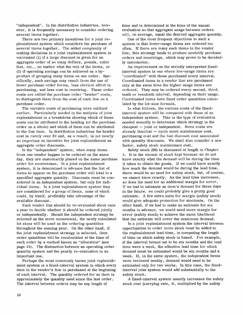
"independent". In the distribution industries, how­ever, it is frequently necessary to consider ordering several items together.

There are two primary incentives for a joint re­plenishment system which considers the purchase of several items together. The added complexity of making decisions in a joint replenishment system is warranted (1) if a large discount is given for an aggregate order of so many dollars, pounds, cubic feet, etc., no matter what the mix of the items, or (2) if operating savings can be achieved as a by­product of grouping many items on one order. Spe­cifically, such savings may result from the use of fewer purchase order forms, less clerical effort in purchasing, and less cost in receiving. These order costs are called the purchase order "header" costs, to distinguish them from the cost of each line on a purchase order.

The variable costs of purchasing were outlined earlier. Particularly needed in the analysis of joint replenishment is a breakdown showing which of these costs can be attributed to the heading (or the purchase order as a whole) and which of them can be attributed to the line item. In distribution industries the header cost is rarely over $2 and, as a result, is not nearly so important an incentive for joint replenishment as aggregate order discounts.

In the "independent" system, when many items from one vendor happen to be ordered on the same day, they are customarily placed on the same purchase order for convenience. In a joint replenishment system, it is determined in advance that the list of items to appear on the purchase order will total to a specified aggregate quantity. Discounts must be con­sidered in an independent system, but only for indi­vidual items. In a joint replenishment system they are considered for a group of items, none of which could, by itself, profitably take advantage of the available discount.

Each vendor line should be re-evaluated about once a year to decide whether it should be ordered jointly or independently. Should the independent strategy be selected as the more economical, the newly calculated lot sizes will be used as the ordering quantities throughout the ensuing year. On the other hand, if the joint replenishment strategy is selected, item order quantities will be recalculated at the time of each order by a method known as "allocation" (see page 18). The distinction between an operating order quantity system and the yearly re-evaluation is an important one.

Perhaps the most commonly known joint replenish­ment system is a fixed-interval system in which every item in the vendor'S line is purchased at the beginning of each interval. The quantity ordered for an item is approximately the quantity used since the last order. The interval between orders may be any length of

16

time and is determined at the time of the annual evaluation so that aggregate usage between orders will, on average, equal the desired aggregate quantity.

One of the most frequent objections to such a system is that lower-usage items are ordered too often. If there are many such items in the vendor line, this strategy tends to produce unwieldy purchase orders and receivings, which may prove to be decided­ly uneconomic.

An improvement on the strictly interpreted fixed­interval system is one where low-usage items are "coordinated" with those purchased every interval. Coordinated items in a vendor line are purchased only at the same time the higher usage items are ordered. They may be ordered every second, third, tenth or twentieth interval, depending on their usage. Coordinated items have fixed order quantities calcu­lated by the lot-size formula.

In what follows, the various costs of the fixed­interval system will be compared with those of an independent system. This is the type of evaluation needed annually to determine which strategy is the cheapest - joint or independent. Some costs are already familiar - cycle stock maintenance cost, purchasing cost and the lost discount cost associated with quantity discounts. We shall also consider a new factor, safety stock maintenance cost.

Safety stock (SS) is discussed at length in Chapter 5. It is the amount of stock kept because we do not know exactly what the demand will be during the time it takes to obtain the goods. If we could know exactly how much the demand would be during the lead time, there would be no need for safety stock, but, of course, we cannot know exactly. As the lead time increases, so does the need for an additional margin for error. If we had to estimate an item I s demand for three days in the future, we could probably give a pretty good estimate. A few extra units for margin (safety stock) would give adequate protection for stockouts. On the other hand, if we had to make an estimate for six months in advance, we would need more margin for error (safety stock) to achieve the same likelihood that the estimate will cover the maximum demand.

In a joint replenishment system the interval between opportunities to order more stock must be added to the replenishment lead time, in computing the length of time on which safety stock is based. For example, if the interval turned out to be six months and the lead time were a week, the effective lead time for which demand must be estimated would be six months and a week. If, in the same system, the independent items were reviewed weekly, demand would need to be estimated only for two weeks. In this case, the fixed­interval joint system would add substantially to the safety stock.

A fixed-interval system usually increases the safety stock cost (carrying rate, R, multiplied by the safety

stock inventory value, SS), while an independent system does not. This is because it usually increases the effective lead time by increasing the length of the period between "looks" at the inventory (that is, it reduces the number of opportunities to buy). Safety stock cost is often the biggest element of increased cost in using a joint replenishment system.

The following costs should also be considered: 1. Cycle stock cost (R L ¥). - Cycle stock, you

will remember, is half the order quantity. The sum of the cycle stock in dollars for all items (L.9.) in the vendor line, multiplied by the carrying rare (R), equals the cycle stock cost. This cost generally is greater under a fixed-interval joint replenishment system (with coordinated items) because the aggre­gate dollar order quantity is greater than the sum of the dollar order quantities in the independent strategy.

2. Purchasing cost. - This consists of two com­ponents:

a. Annual header cost (NA). This is the cost per header (A) multiplied by the number of headers per year (N). This cost will usually be less under joint replenishment because the system often reduces the frequency of purchasing.

b. Line cost (na). This is the unit cost of a line (a) multiplied by the number of lines per year (n). This cost will usually be decreased if the fixed-interval system permits the use of coor­dinated items.

3. Discount savings (S$ d .. ~:> or lost discount cost. - When an available discount is not taken, potential profit is lost to the company. The cost of losing discounts should be considered cost for items purchased in such a manner. For vendors whose discounts are made, the difference may be termed a "discount savings" and subtracted from all the other costs. The value is computed by multiplying the discount rate (d~) applicable through use of the system by the annual sales for the vendor in dollars (S$)' These savings, where they exist, are the primary justification for a joint system over independent purchasing.

4. Annual cost of items (at undiscounted prices) (S$)' - The annual dollar amount paid the ven­dor is the sum of the unit purchase cost for each item multiplied by the annual sales in units for each item.

The steps for deciding which system to use are as follows:

1. Compute the ordering interval necessary to achieve each price break offered for an aggregate order. For example, assume a vendor has one price break, Q, for which he gives a discount, de.(' If the distributor sells S$ per year, he would order ~ times

Q per year to receive the do< discount.

2. Compute the valid intervals between price breaks. The method is not unlike the one explained in the previous section for an item quantity discount. The formula to determine the intervals for a vendor

line is I 2 (A + ka) S$

-V R (1 - dD( ) where

A = purchase order header cost in dollars. k = number of items in a vendor line. a = purchase order line cost. S$ = annual sales in dollars for the vendor line. R = maintenance cost rate expressed as a decimal. d..<, = applicable discount. 3. Cost the valid joint replenishment strategies

for the intervals calculated in steps 1 and 2. Sum the costs and determine which joint strategy is the cheapest.

4. Cost the independent strategies for the same elements. There are two such strategies to be costed:

a. Those with lot sizes calculated with line pur­chase order cost only. *

b. Those with lot sizes calculated with header plus line purchase order cost. *

5. Select the cheapest strategy from steps 3 and 4. An example will illustrate the process. Assume

a vendor has the following characteristics: Annual sales, in cost $ excl. disc. (S$) $120,000 Number of items in line (k) 30 Purchase order header cost (A) $1. 00 Purchase order line cost (a) $ . 50 Maintenance cost rate (R) .20 One joint discount (deo< ) 5% If order aggregates to a quantity (Qo< ) $10,000 Max. annual discount savings (do<. S$) $ 6,000 Min. annual payment to vendor (S$ - do<. S$) $114,000 Variable annual cost All costs less $114,000 Review 52 times a year. Review time (RT) = 1 week Lead time (LT) = 1 week

Step 1: Compute the ordering interval necessary to achieve each total order price break.

a. At the price break of $10,000, we must order once a month (12 times per year) to receive the 5% discount, since $120,000 is sold per year.

*The line cost strategy is applicable where header costs are "fixed"

- that is, where it has been determined that at least one item will be ordered on every occasion on which it is feasible to place an order

with a particular vendor, so that the annual header cost cannot vary.

For example, if the distributor reviews items no more often than

weekly (52 opportunities to buy per year) and the vendor line gen­

erates 100 lines per year, the line cost independent strategy is

applicable. Conversely, if the number of purchase order lines

generated for a vendor line is less than the number of opportunities

to buy, the header cost is variable and should be considered as part

of the purchasing cost. Specifically, if the distributor reviews items

only weekly (52 opportunities to buy per year) and the vendor line

generates 20 lines per year, the header-plus-line-cost lot sizes are

applicable.

17

b. The base price (no discount) is available at the "0" price break. Joint ordering should also be considered at this undiscounted price with the smallest possible joint ordering aggregate order quantity. The joint strategy that orders at every opportunity to buy produces the smallest possible aggregate order quantity. In our example, since the distributor "reviews" all items only once a week, the smallest dollar value that could be ordered jointly is $120,000 =

52 $2,307.19 with an interval of one week (52 times a year).

Step 2: Compute the valid intervals between price breaks with the formular--___ _

2 (A+ka)S$ R(I-dc-< )

a. Between the $ "0" and $10, 000 discount breakpoint

/2($1. 00 + 30 [$. 50J ) $ 120,000 = $4,381. 78

-J .20 (1-0) Since sales are $120,000 per year,

$120,000 . = 27.4 times per year.

$4,381. 78 Since purchasing can only be done weekly, this is rounded to a whole number of weeks (2), or 26 times per year. This yields an aggregate quantity of $120,000 = $4,615.38 each order.

26 b. Above the $10,000 discount breakpoint

2($1. 00 + 30 [$. 50J) $ 120,000 _ -----=------==------ - $4, 495. 61

.20 (1-.05)

But, in order to qualify for the 5% discount, the purchaser must order $10,000 or over. If $4,495.61 were ordered, NO discount would be allowed. Therefore, this strategy is invalid and may not be considered.

Step 3: Cost the valid joint replenishment strate­gies for the intervals calculated in steps 1 and 2, and select the cheapest of these.

In order to cost, it is necessary to know the safety stock required for the different strategies. Through a calculation not detailed here, these safety stocks have been determined as follows:

a. Joint ordering at the $10,000 price break (during the lead time plus one month fixed interval, LT + FI) requires $16, 000 of safety stock.

b. Joint ordering at the $0 price break (during the lead time plus one week fixed interval, LT + FI) requires $6,000 of safety stock.

c. Joint ordering at the interval computed between the $0 and the $10,000 price break (during the lead time plus two weeks fixed interval, LT + FI) requires $9,000 of safety stock.

Figure 14 shows the costing for the three intervals calculated in steps 1 and 2.

18

Summarized, the annual joint replenishment costs are as follows: InteIVal Joint OQ 1 week $ 2,307.69 2 weeks $ 4,615.38 1 month $10,000.00

Annual Total Cost $122,104.00 $122,677.54 $118,420.00

Annual Variable Cost $8,104.00 $8,677.54 $4,420.00

The one-month interval with $10,000.00 aggregate order quantity is the cheapest joint strategy.

Step 4: Cost the independent strategies The safety stock needed for the specified level of

service for both independent strategies (during the lead time plus review time, LT + RT) = $6,000. Figure 15 illustrates the costing for the two independ­ent strategies. Summarized, the annual independent costs are as follows:

Average Strategy Aggregate OQ Line cost lots $2,307.69 Header-plus-

Annual Total Cost $122, 101. 00

Annual Variable Cost $8,101. 00

line-cost lots $2, 307. 69 $122,236.20 $8,236.20

Step 5: Select the cheapest strategy from steps (3) and (4).

Strategy

(1) Independent line cost lots

Average Aggregate

Order Quantity

$ 2,307.69

(2) Independent $ 2, 307.69 header-plus-line­

cost lots

(3) Cheapest of $10,000.00

joint strategies -inteIVal 1 month

Annual Total Annual Cost

$122, 101.00 Variable Cost

$8,101.00

$122,236.20 $8,236.20

$118,420.00 $4,420.00

The cheapest strategy is the joint system with an interval of one month.

Once a joint replenishment system has been selected, a day-to-day allocation method must be set up. This system decides how much of each item should be ordered each interval. Sales rates for an item will change from one time period to another. The allocation system orders by item approximately what was used since the last order and so considers changing sales rates.

Then the system checks to see whether the sum of these items aggregates to the quantity specified as most economical when the joint strategy was selected. For example, the desired discount break might be $4, 000, yet the total usage for all items since last interval may amount to only $3,500. Somehow, the total order quantity must be increased $500 to make the discount. The allocation system will distribute the $500 amount over the items in the line.

Two systems of allocation will be discussed. The first is the method for a fixed-interval system as has been defined earlier in this section. Probably the best known allocation method is to add an equal time supply to the basic requirement for each item. This system is easiest to understand and calculate. Every item has its order quantity increased by some factor

A B C D E

Safety Stock Cycle Annual Annual Annual

Interval Cost Stock Cost Header Line Discount

Cost Cost Savings

R'SS R·I i LT+F1 NA na do<; S$

Price break = SSLT+F1 = I~= $5,170 .N = 1':: n -,34S Since J"1'OQ-

$10,000. $16,000 2 @:l$1 (cil$.50 $10,000,

Results in @:l20% @:l20% d"" = 5%

one-month

interval. $3,200.00 $1,034.00 $12.00 $174.00 $6,000.00

Price break = SSL T + FI =$6,000 I i= $1,935 N=52 n- 930 Since JTOQ-

$0. @:l20% @:l$1 @:l$.50 $2,307.69,

Results in @:l20% d .... = 0

one-week $1,200.00 $387.00 $52.00 $465.00 ° interval.

Between the SSLT+FI=$9,000 I~= N=26 n= 780 Since JTOQ-

$0 and $10,000 @:l$1 @:l$.50 $4,615.38,

price break. @:l20%

$2,307.69 d~=O

Results in two- @:l20%

week interval. $1,800.00 $461.54 $26.00 $390.00 0

Figure 14. Annual cost to handle all the items in a vendor line. Example illustrates three fixed-interval joint replenishment systems. Asterisk denotes the

cheapest system.

A B C D

Safety Stock Cycle Annual Annual

Cost Stock Cost Header Line Strategy Cost Cost

R' SSLT+RT R·I q NA na 2

SSL T + RT = $6, 000 I i=$2, 180

N= 52 n = 826

Line Cost @:l20% lots @:l20% @:l$1 @:l$. 50

~2~ $1,200.00 $436.00 $52.00 $413.00

Header-Plus- SSLT + RT=$6, 000 I.3. =$3 706

N- 52 n == 486 Line-Cost 2 ' Lots

@:l20% @:l20% @:l$1. 00 @:l$. 50

~ 2 (;+a)s $1,200.00 $741. 20 $52.00 $243.00

Figure 15. Annual cost to handle all the items in a vendor line. Example illustrates two independent strategies.

E

Annual

Discount

Savings

doc; S$

Since avg.

aggregate OQ=

$2,307.69,

do<: = 0

° Since avg. aggregate OQ= $2,307.69,

d =0 "<

0

F G H

Annual Total Total Cost of Annual Annual

Item Cost Variable

(at base prices) Cost

S$ C (C-$114,000)

$120,000.00 $118,420.00 $4,420.00*

$120,000.00 $122,104.00 $8,104.00

$120,000.00 $122,677.54 $8,677.54

F G H

Annual Total Total

Cost of Annual Annual

Items Cost Variable

(at undiscount- Cost

ed prices)

S$ C (C-$114,000)

$120,000.00 $122,101. 00 $8,101.00

$120,000.00- $122,236.20 $8,236.20

19

times its average daily usage, so that the total order fulfills the aggregate requirement. The hope, of course, is that the balances for all items will be re­duced (in time supply) at the same rate; if sales rates were constant, it would then be possible to enter exactly the same order each time. Since sales rates vary, however, it is inevitable that some items will run out or reach a dangerously low point before ~he aggregate sales are enough to warrant placing another complete order. A better solution for a fixed-interval system is to add more stock for those items that are likely to run out first. This can be done using statis­tical techniques (see Chapter 5). It is technically described as equalizing the probability of stockout.

The second system of allocation is the method for

20

an order-point joint replenishment system. Under this system, all items are ordered when the first item needs to be ordered. It might appear that this would either balloon inventory or make it impossible to make the preferred aggregate quantity, but such is not the case when the system is set up on a statistical basis. The basis of allocation is to equalize the time of run­out by ordering in equal time supply above a statis­tically computed safety stock. The total costs of an order-point joint replenishment system are approx­imately the same as for a fixed-interval system. The choice between the two is largely dependent upon the environment of a particular concern.

IBM's IMPACT Computer Program Library in­cludes routines for both methods of allocation.

CHAPTER 4: ORDER POINT

Recall that control of an item in inventory hinges on two fundamental questions: (1) when to buy (order point) and (2) how much to buy (order quantity).

The "how much" question was discussed in the chapter entitled "Order Quantity" (page 9). In this chapter the "when" question will be dealt with. It is convenient to answer this question in the form, "When stock is reduced to 100 it is time to buy." The number 100 (or any other appropriate value) is called an order point. Recall that the order point is the stock you have on the shelves or on order when you order, while the order quantity is the additional stock you are telling the vendor to ship. During the time it takes the new shipment to arrive, the stock which was on hand will be depleted. The order point is set to plan for this depletion, recognizing that the alternative of waiting until an item is actually out of stock is usually undesirable. To set order point, the following factors must be taken into account:

1. Lead time 2. Review time 3. Forecast of usage per time unit 4. Measure of forecast error The fourth factor is the most important single

concept of scientific inventory management. It is more likely to be totally unfamiliar to the reader than the other three. The four factors will now be considered one at a time.

Lead Time

Lead time starts when an order is written and ends when the material is received. It includes the time it takes the buying company to process a purchase order, and time for the order to travel in the mail to the vendor. Further, it includes vendor proc­essing time and transit time for shipment, as well as the time for the receiving firm to put the goods on the shelf ready for issue.

Inventory is, of course, reduced with the passage of time, as shown in Figure 16. Under ideal circum­stances, it would be desirable to run out of an item just as a new shipment is received. The happy result would be no lost sales and no excess inventory. To avoid lost sales, it is obviously necessary to place an order one lead time before running out. This reintroduces. the first fundamental question: When should the order be placed? Or, in our newer terminology, what should the order point be? It must include expected usage (or demand) during the lead time.

Order point = lead time x usage Clearly, then, an accurate knowledge of the lead

time is required. If the usage for an item is 50 per time unit, and lead time is two time units, order

point is 100 (2 x 50). This is illustrated in Figure 17. If lead time were only one time unit, order point would be 50. If lead time were 1. 5 time units, order point would be 75. Setting of order point simply consists of looking ahead one lead time to see when the present supply of goods would run out.

Note that the longer the lead time, the higher the order pOint. (For the moment, the obvious fact that a vendor's lead time may vary from time to time will be bypassed.)

INVENTORY LEVEL

ORDER

~

\.'-----~\~----,~ LEAD TIME

TIME

Figure 16. Inventory depletion with time

100

INVENTORY LEVEL

50

FEB

ORDER ~RECEIVED

Figure 17. Effect of lead time on order point

ORDER POINT

21

Review Time

"Review" means comparing an item's order point with the available stock for that item. "Available stock" is a fundamental concept:

Available stock = stock on hand + stock on order -backorders

The comparison of available stock with order point is made to determine whether it is time to buy. The buyer is not required to buy an item at each review, but is simply considering the possibility.

It is common practice to review the inventory on a periodic basis. A periodic review system reduces the number of opportunities to buy per year to 52 for weekly review, or 12 for monthly review. Even if review is not periodic, the number of opportunities to buy will never exceed the number of working days per year, since it is unlikely that a company places more than one order per day with its vendors.

Since the buyer does not know the inventory level of an item during the period between reviews (except in an emergency), he must allow for the usage which will take place between reviews. If he fails to do so, he could fall below lead-time usage before the item is reviewed again, with the attendant certainty of a stockout. Review time must be added to the lead time in setting order point:

Order point = (lead time + review time) x usage This may be clarified by an example of what

happens if review time is not considered. Assume that an item is being reviewed weekly on Monday. If lead time is two weeks and usage per time unit is 50, order point is 100 without the addition of review time. Suppose that available stock is 101 at the time of a particular review; since this is above order point, no order would be placed. During the succeeding week, the normal usage of 50 will reduce the available stock to 51, at the time of the next weekly review. An order would now be placed, but since lead time is two weeks, the item will be out of stock during the second week. The avoidance of such stockouts re­quires that review time be added to the lead time, making order point 150 in the case cited.

Random access files frequently make it economical to review the available stock at the time of each transaction, which is often referred to as "continuous" review. In such a case, review time is effectively zero, so order point is lower than with periodic review.

Forecast of Usage per Time Unit

In discussing the effect of lead time and review time in setting order point, it was assumed that the rate of usage was known. Normally, of course, you do not know, but have to forecast (or guess), how fast an item will sell. This is not a forecast for the

22

business as a whole, but for each item. Neither is it a long-range forecast, but only to cover the lead time (and possibly review time), which is all that need concern you in setting order point. For many items it is common, and appropriate, to base a forecast of future sales on past behavior. This is particularly true of "stable" items which have been in the line for some time. Various techniques of forecasting item sales are discussed in a subsequent section. For the moment, assume that the forecast of usage will be a type of average based upon history. This forecast, projected through lead time and review time, will be used in determining order point. The only trouble is that the forecast might be wrong.

Measure of Forecast Error

If the forecast is too low (exceeded by usage), you are faced with lost sales. In fact, since the forecast is an average, you can reasonably expect it to be too low about half the time. A good forecast will also be too high about half the time, but you are more con­cerned about the low side, which means you won't be able to ship the goods. To allow for this contingency, the order point might be arbitrarily raised, thus creating a buffer or safety stock which is dipped into when the forecast is too low. Adding this safety stock has the effect of increasing the average inventory, with an associated increase in maintenance cost. This additional inventory may be considered a good investment up to some reasonable pOint, because of the sales that would otherwise have been lost. Only beyond this reasonable point is there overstock.

To better understand how this safety stock might work, look at the same item twice, first without safety stock (Figure 18) and then with it (Figure 19).

100

INVENTORY LEVEL ~o

TIME

~ ORDER RECEIVED

Forecast usage per time unit: 50

Lead Time: 1 time unit

Review Time: 0 (continuous)

Order Point: 1 x 50 = 50

- -- - - -- ORDER POINT WITHOUT SAFETY STOCK

LEAD TIME

Figure 18. Inventory behavior without safety stock

____ ORDER RECEIVED

ISO

100 - - - - - - - - - - - - - - - ORDER POINT WITH SAFETY STOCK

INVENTORY LEVEL ~+-__________ ~L-______ ~ ________ -.

SAFETY STOCK

~I LEAD TIME

TIME

Forecast usage per time unit: SO

Lead Time: 1 time unit

Review Time: a (continuous)

Order Point without safety stock: 1 x SO = SO

Safety Stock: forecast usage for 1 time unit = SO

Order Point with safety stock: SO + SO = 100

Figure 19. Inventory behavior with safety stock

In both cases lead time is 1. Note that with no safety stock, when sales are exactly equal to forecast, the inventory is reduced to zero just as the new ship­ment comes in. Similarly, with safety stock, the level where you would start issuing safety stock is just reached when the new shipment comes in. Both of the foregoing statements are true only because the forecast usage of 50 per time unit was exactly right. If, in fact, usage had been 60 per time unit, you would have lost sales in the first case, and used 10 units of safety stock in the second. The safety stock is protection against such an error of 10 units in forecasting demand.

It has been common for a business to specify that safety stock will be the usage for one month (or whatever time interval is pertinent). A better basis will be suggested: Suppose that in the last five years the average usage per month was 50, but the maxi­mum usage observed was 60 per month. In such a case, setting an arbitrary safety stock of one month's usage clearly results in carrying excess inventory. If the future bears any relation to the past, it is reasonably certain that the forecast will never be too low by more than 10 units. Obviously, 40 units of this item have been maintained unnecessarily for five years ... at considerable expense. If safety stock is set as a function of forecast error (no greater than 10 in this case), you can expect to save money as well as satisfy maximum reasonable demand. (Any attempt to satisfy all possible demands will invariably meet with failure or bankrupt the business. )

If the forecast were perfect, no safety stock would be necessary. Recognizing that it cannot be 100% accurate, measure how wrong it is, and let safety stock vary with the error. Thus, the poorer the forecasts, the larger will be the safety stock.

Measuring forecast error and using it to set safety stock is the most significant concept of scientific inventory management. This is particularly true in distribution industries where safety stock typically forms the bulk of the inventory under present controls.

This section can be summarized by restating the order point formula:

Order point = (lead time + review time) x forecast of usage per time unit + safety stock

where safety stock is based on a measure of fore­cast error.

Forecasting and measuring the forecast error are discussed in detail in the next two chapters.

23

CHAPTER 5: SERVICE AND SAFETY STOCKS

Customer satisfaction is one of the most precious assets a business enterprise can have. Certainly one of the major positive influences in a customer's thinking is a high probability that goods he orders will be delivered. All other things being equal, the customer will tend to favor the supplier who most often provides the merchandise he has ordered. If a retailer can place heavy reliance on his distributor, he can safely operate with less inventory - a clear­cut saving for him. The distributor commonly has extremely high service objectives because there is usually a competitor who is equally convenient for the customer. As a result, back orders are rare, and the likely consequence of being out of stock is a lost sale. It is virtually impossible to reach agree­ment on the precise cost of a lost sale, particularly if one tries to place a value on goodwill. It might seem at first glance that the minimum cost is the gross profit lost, but some companies feel it is less than that since they have not packed it, etc.

While there are several ways of defining customer service, they all hinge on some measure of how effectively demand is met, and are most often ex­pressed as a percentage figure. For the moment, we shall define customer service as the percentage of dollar demand which is filled routinely from goods on the shelf.

$ shipments Service % = $ d or ers

Conversely:

$ shipments Stockout % = 100 - ----­

$ orders

It is ~ possible to achieve 100% service for all items, for any of several reasons: the vendor's inability to supply, selection or picking errors in your warehouse, clerical errors, or the failure to issue a picking slip because the inventory record erroneously shows an item as out of stock. The last three problems may be reduced in frequency by tighter administrative controls, but are in no way influenced by buying decisions.

Of prime concern to scientific inventory manage­ment is better regulation of those stockouts which are attributable solely to buying decisions - more specifically, the answer to the "when" question.

Statistical theory can be used to produce decisions aimed at achieving a specific service level. To specify a desired level of service, management needs to be informed in advance of the cost implications of various pOlicies. Such a guide to policy setting can be provided in the form of the graph in Figure 20. Note that the additional inventory required to improve service becomes progressively greater in moving to

24

INVENTORY INVESTMENT

(IN 1,000'5)

600

500

400

500

200

100

SERVICE PERCENl'AGE

Figure 20. Inventory investment required for various service levels

very high levels of service. We shall now introduce a statistical concept which

is fundamental to scientific inventory management.

Playing the Odds

When you buy auto insurance you realize that the selling company has no assurance that it will make money on your policy. They know, however, that most of their policyholders will sustain only minor damage, if any. They are taking a calculated risk which can be assessed with sufficient precision to figure a premium right down to the penny. Any executive will concede that insurance companies make a profit by "figuring the odds" - that is, by making intelligent use of the laws of chance. It will probably be a more novel idea to suggest that the same tech­niques of evaluating risks can vastly improve the management of inventories. Fortunately, you need not become a professional statistician, but can profit greatly by borrowing only one or two of their basic principles.

Since the statistician likes to describe things quantitatively, he habitually measures some charac­teristic of interest to him to accumulate a sample of measurements. To him, a sample can be described by a series of numbers - for example, intelligence quotients or weights for a group of people, the temperature measured at noon every day, sales of an item during a week, or errors in periodic forecasts of item sales.

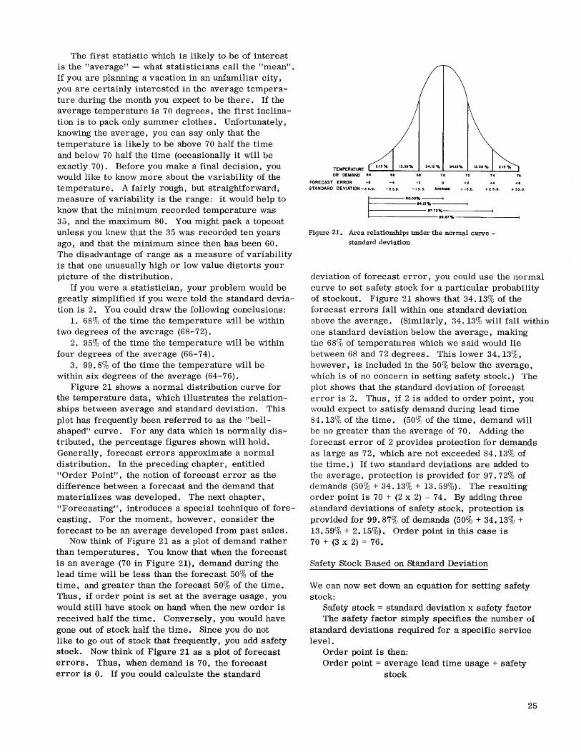
The first statistic which is likely to be of interest is the "average" - what statisticians call the "mean". If you are planning a vacation in an unfamiliar city, you are certainly interested in the average tempera­ture during the month you expect to be there. If the average temperature is 70 degrees, the first inclina­tion is to pack only summer clothes. Unfortunately, knowing the average, you can say only that the temperature is likely to be above 70 half the time and below 70 half the time (occasionally it will be exactly 70). Before you make a final decision, you would like to know more about the variability of the temperature. A fairly rough, but straightforward, measure of variability is the range: it would help to know that the minimum recorded temperature was 35, and the maximum 80. You might pack a topcoat unless you knew that the 35 was recorded ten years ago, and that the minimum since then has been 60. The disadvantage of range as a measure of variability is that one unusually high or low value distorts your picture of the distribution.

If you were a statistician, your problem would be greatly simplified if you were told the standard devia­tion is 2. You could draw the following conclusions:

1. 68% of the time the temperature will be within two degrees of the average (68-72).

2. 95% of the time the temperature will be within four degrees of the average (66-74).

3. 99.8% of the time the temperature will be within six degrees of the average (64-76).

Figure 21 shows a normal distribution curve for the temperature data, which illustrates the relation­ships between average and standard deviation. This plot has frequently been referred to as the "bell­shaped" curve. For any data which is normally dis­tributed, the percentage figures shown will hold. Generally, forecast errors approximate a normal distribution. In the preceding chapter, entitled "Order Point", the notion of forecast error as the difference between a forecast and the demand that materializes was developed. The next chapter, "Forecasting", introduces a special technique of fore­casting. For the moment, however, consider the forecast to be an average developed from past sales.

Now think of Figure 21 as a plot of demand rather than temperatures. You know that when the forecast is an average (70 in Figure 21), demand during the lead time will be less than the forecast 50% of the time, and greater than the forecast 50% of the time. Thus, if order point is set at the average usage, you would still have stock on hand when the new order is received half the time. Conversely, you would have gone out of stock half the time. Since you do not like to go out of stock that frequently, you add safety stock. Now think of Figure 21 as a plot of forecast errors. Thus, when demand is 70, the forecast error is O. If you could calculate the standard

~;M~~~TN~E .'-4 _____ •• L-.3_."_%.......L._3_4 .• 3_%_7L..0 _34_.13_'lb-L.._.3_.51_%-L.._----J

FORECAST ERROR -8

STANDARD DEVIATION -3 S.D. -2S.D. AVERAGE

t-----80.00%----i t------84.13%-----4

+2 S.D.

t------- .7.72%----_

1--------••.• 7%------....

Figure 21. Area relationships under the normal curve -standard deviation

deviation of forecast error, you could use the normal curve to set safety stock for a particular probability of stockout. Figure 21 shows that 34.13% of the forecast errors fall within one standard deviation above the average. (Similarly, 34. 13% will fall within one standard deviation below the average, making the 68% of temperatures which we said would lie between 68 and 72 degrees. This lower 34.13%, however, is included in the 50% below the average, which is of no concern in setting safety stock.) The plot shows that the standard deviation of forecast error is 2. Thus, if 2 is added to order point, you would expect to satisfy demand during lead time 84. 13% of the time. (50% of the time, demand will be no greater than the average of 70. Adding the forecast error of 2 provides protection for demands as large as 72, which are not exceeded 84.13% of the time.) If two standard deviations are added to the average, protection is provided for 97.72% of demands (50% + 34. 13% + 13. 59%). The resulting order point is 70 + (2 x 2) = 74. By adding three standard deviations of safety stock, protection is provided for 99.87% of demands (50% + 34.13% + 13.59% + 2.15%). Order point in this case is 70 + (3 x 2) = 76.

Safety Stock Based on Standard Deviation

We can now set down an equation for setting safety stock:

Safety stock = standard deviation x safety factor The safety factor simply specifies the number of

standard deviations required for a specific service level.

Order point is then: Order point = average lead time usage + safety

stock

25

The interesting thing about the standard deviation is that the percentage relationships always hold regardless of the particular values for average and standard deviation. If our forecasts are exceptionally good, the forecast errors will be very small, and the safety stock can be correspondingly small, even to give very high service. For example, if average usage were 1,000, and standard deviation of forecast error were 10, our order point would be only 1,030 to yield 99. 87% service. On the other hand, if it is very difficult to forecast, so that forecast error is large, we end up with a large safety stock. Thus, if average usage were 1,000, but standard deviation of forecast error were 100, order point for 99.87% service would be 1,300. Figure 22 gives safety stocks and order points for additional sample data. Examination of the data suggests two conclusions:

1. A poor forecast creates a need for larger safety stocks. Accordingly, it is worth some effort to get good forecasts. (This will be discussed in the next chapter.)

2. A uniform level of service can be achieved only by taking the variability of the distribution into account. Any scheme which bases safety stock on a fixed time supply fails to do this, and will result in overstocking some items while other items will have frequent shortages because the safety stock is too small.

Calculating the Standard Deviation

It has been suggested that service and safety stocks can be much more effectively controlled through the use of standard deviation. The classic formula for calculating it is:

n

Standard deviation = i=l n

The formula is imposing but can be solved in four steps:

1. Take the deviation of each forecast error from the average forecast error.

2. Square each deviation. 3. Divide the summed squares by the number of

errors measured. 4. Extract the square root. From a computing point of view, calculating stand­

ard deviations is not appealing, because division and extraction of square roots are among a computer's slowest operations.

An Approximation of Standard Deviation

Fortunately, there is a good way of approximating standard deviation which requires substantially less computing time. For a normal distribution, it is just as accurate as standard deviation. This measure is called "mean absolute deviation" (MAD). The relationship between standard deviation and MAD is such that:

Standard deviation = 1. 25 x MAD Thus, knowing the MAD, you multiply by 1. 25 to

get the standard deviation. The normal distribution curve provides the means to find the safety factor for a desired level of service. A continuing need to multiply can be avoided by simply refiguring the normal curve areas for MAD instead of standard deviation. This has been done in Figure 23. Figure 24 shows representative safety factors to achieve a given level of service with MAD. Safety stock is given by:

Safety stock = safety factor x MAD As before, safety factor simply specifies the

number of MAD's to yield a specified level of service.

Safety Stocks for Various

A verage Lead Standard Deviation Levels of Service Order Points for Various Item Time Usage of Forecast Error 50.00% 84.13% 97.72% 99.87% Levels of Service

SAFETY FACTOR 0 1 2 3 50.00% 84.13% 97.72% 99.87%

1 100 0 0 0 0 0 100 100 100 100 2 100 5 0 5 10 15 100 105 110 115 3 100 10 0 10 20 30 100 110 120 130 4 100 25 0 25 50 75 100 125 150 175 5 100 75 0 75 150 225 100 175 250 325 6 100 100 0 100 200 300 100 200 300 400 7 500 20 0 20 40 60 500 520 540 560 8 500 100 0 100 200 300 500 600 700 800

Figure 22. Order points for sample items

26

2.15% 13.511% 54.15% 34.150/0 15.59%

MAD -3.75 -2.50 -1.25 AVERAGE + 1.25

1----- 50.00%------1

f------ 84.13"/.-------i

+2.50

1-------97.72%--------1

+5.75

1--------99.87%---------1

Figure 23. Area relationships under the normal curve - mean

absolute deviation (MAD)

Safety Factor

0.00

1. 00

1. 25

2.00

2.50

3.00

3.75

% of Order Cycles with No Stockout

50.00

78.81 84.13

94.52

97.72 99. 18 99.87

Figure 24. Safety factors for service levels using MAD

(service based on frequency of stockout)

Now we had better determine how to calculate MAD. "Mean", of course, is just another term for average. "Deviation" simply means the difference between an individual observation and the average of all observations. "Absolute" means that we shall always consider the deviation as positive, ignoring any minus signs. The formula is:

n

Mean absolute deviation = i=l n

The formula can be solved in two steps: 1. Take the deviation of each forecast error from

the average forecast error, without regard to sign. 2. Divide the summed deviations by the number of

errors measured. While the square root extraction required for

standard deviation has been eliminated, a division is still involved. A better solution will be presented in the section on forecasting.

If you have understood the discussion of statistical concepts presented to this point, you have done two things:

1. Learned as much about statistics as you will need to.

2. Understood the most important single concept of scientific inventory management.

Ways of Measuring Service

We have spoken of basing safety stock on a statistical measure of forecast error, the mean absolute devia­tion. To achieve a given level of service, a multi­plier, the safety factor, was used, the value of which was obtained from the normal curve. It could be said, for example, that demand would not exceed average demand plus 2.50 MAD's 97.72% of the time. There is now a need to be more precise about what kind of customer service will result from such a rule.

To illustrate, let us assume that you have picked a safety factor to yield 98% service. The rule says that after you have reached order point (and issued an order), you can expect to fill all customer orders during the lead time 98% of the time. Two percent of the time, you can expect to run out before the new shipment arrives. There is no way of telling how large the shortage will be; whether it is one unit or many units, it makes an equal contribution to the expected 2% of stockouts. In other words, you have an estimate of how frequently you will run out, but no estimate of the quantity or size of unfilled orders. The expected frequency of stockout is related to the frequency of orders to a vendor. That is, when you place 100 orders for a particular item, it is probable that 98 of them will be received without a stockout occurring. If you ordered only once a year, there would be stockouts in only 2 years out of 100. If you ordered weekly, you would have a stockout about once a year. To sum up, the frequency of stockout per order cycle will be the same for all items with the same safety factor.

The measure of service which has been under discussion is quite likely to be different from that which many companies are presently using. This has been done because it is easier to relate to statistical concepts on first exposure. Beginning with the next paragraph, a more usual measure of service will be presented. Let us restate the measure you know now before going on to the second one: Safety factor is set to provide a level of service measured as the percentage of order cycles during which no stockout occurs.

Some managements prefer to satisfy a specified percentage of demand, which is quite a different measure of service than frequency of stockout. To do so requires a different value of the safety factor for each item. One of IBM's IMPACT Computer Programs determines the appropriate value using the table in Figure 25 and the follOwing formula:

order quantity Service function = A f f (1 - desired

M D 0 orecast . error during lead time

serVICe level)

27

Service function is simply an intermediate value calculated to provide entry to the table in Figure 25.

Safety Factor Service Function

0.0 .4998

0.2 .4062

0.4 .3252

0.6 .2561

0.8 .1985 1.0 .1510 1.2 .1131 1.4 .0829 1.6 .0600 1.8 .0425 2.0 .0294 2.2 .0199 2.4 .0134 2.6 .0088 2.8 .0056 3.0 .0035 3.2 .0023 3.4 .0015 3.6 .0009 3.8 .0005 4.0 .0004

Figure 25. Service function for the normal distribution of forecast errors

The order quantity and MAD interact to affect the percentage of demand filled routinely. If order quan­tity is large in relation to forecast error, the order quantity alone will provide protection for some time after goods are received. This is illustrated in Figure 26 where item A has a larger order quantity in terms of time supply than item B. Taking this into account will yield a lower safety factor for item A than for item B, while satisfying the same percentage of demand for both items.

OR[ER OUANTITY

= 6 MOS. SUPPLY

ITEM a, ORDER QUANTITY

= I MO. SUPPLY

Figure 26. Exposure to stockout of items with different order quantities

28

Examples: Item A Order quautity: 600 (annual usage is 1,200, so this

represents a six-month supply) MAD of forecast error during lead time: 75 Desired service: 95% Service function: ~~O (1 - .95) = .4

From Figure 25, safety factor for service function of .4 = .2

Item B Order quantity: 100 (annual usage is 1,200, so

this represents a one-month supply)

MAD of forecast error during lead time: 75 Desired service: 95% Service function = 100 (1 - . 95) = . 0625

75 From Figure 25, safety factor for service function

of.0625=1.6

Note that the safety factor for this measure of service is lower than when based on frequency of stockout. In aiming to satisfy a given percentage of demand, it is not possible to know how frequently a stockout will occur, nor how large any particular stockout will be. The thing you are specifying is that over a period of time, some desired percentage of demand will be filled from goods on the shelf.

Summary

When goods are ordered from a vendor, there is always uncertainty about customer demand rate during the interval prior to receipt. Order point is set to allow for this uncertainty. If order point is based on a forecast of average usage alone, stockoutscan be anticipated during about half the replenishment cycles. To get better service requires raising order point by adding safety stock. This safety stock should be based on a measure of forecast error rather than some fixed multiple of average usage. Statisti­cal concepts make it possible to find a safety factor which will yield a specified level of service. Two measures of service have been presented:

1. Frequency of stockout, without regard to size or number of unfilled orders. The safety factor is taken directly from the normal curve.

2. Size of stockout without regard to frequency. This measure of service aims at filling a given per­centage of demand from the shelf. The relationship between order quantity and forecast error is con­sidered in setting the safety factor, through use of a formula and table.

CHAPTER 6: FORECASTING

Previous chapters of this manual have developed the need for a forecast of average usage and a measure of forecast error to set order point. That a good forecast is desirable was evidenced by the reduction in safety stocks which accompanied reduced forecast errors. This chapter becomes quite detailed in discussing one method of forecasting; the executive may be satisfied by skipping from the portion entitled "Controls" to the next chapter, "System Implemen­tation", page 41.

It is useful to make a distinction between predic­tion and forecasting. Prediction is judgmental -guessing what will happen in the future with no directly related events in the past on which to base such a guess. It is strictly intuitive. Predictions were made in the case of such items as compact cars, pet insurance, new toys, colored sidewall tires, etc.

Forecasting, on the other hand, is extrapolation of the past into the future. Guessing or estimating is still involved but there is a past series of numbers on which to base the estimate. Further, there is no reason to think that the number series will be subject to changes other than those inherent in general economic conditions and the capacity of consumer demand. There are no laws, but there do seem to be consistencies.

A good forecast should have stability in the face of random fluctuations. At the same time, it should be responsive to real changes in demand. These two requirements are in conflict with each other, and which of the two should receive greater weight will depend on the business climate of a particular firm and on management's inclinations. Inappropriate emphasis on either may adversely affect service and/ or inventory. Generally, a systematic and consistent balancing of the two will achieve superior results over intuitive forecasting because of a human tenden­cy to overcompensate. A well planned forecasting system will not overreact to the unusual or novel event, as people tend to do.

Whether the method is intuitive or systematic, there are two main ways of arriving at a forecast:

1. Extrinsic. This is more appropriate in fore­casting sales of the total product line than of indi­vidual items. It is assumed that a correlation exists between the thing being forecast and some external statistic such as gross national product, housing starts, birth rate, consumer index, industrial inven­tory levels, new car registrations, etc.

2. Intrinsic. The intrinsic approach is particu-1arly applicable to the forecasting of demand for individual items. It assumes that the best way to tell how an item will sell in the future is to look at its past behavior (or that of a closely related item).

The bulk of the items in an inventory fall into one of three basic demand patterns: constant, trend or seasonal. While there are exceptions, of course, the great majority of items in a product line can be placed in one of these three categories.

Figure 27 shows monthly shipments of cat food over a period of several years. Though there are substantial fluctuations among various periods, they are random - that is, there is no detectable pattern to them. The fact that sales are below (or above) average for one month does not permit any specific inference about sales during the coming month. The best estimate of future demand is the average of past demands plus an allowance for forecast error (safety stock) . Such a demand pattern may be classed as "constant" or "horizontal". It is characterized by an essentially stable level of demand with random fluctuations or "noise".

Under some conditions, the long range level of demand may exhibit a consistent pattern of increase or decrease - commonly called "trend". Since an average is at the midpoint of the history comprising it, that figure will not be current where a trend exists. Caution must be used in applying techniques which compensate for trend, however, as they may inter­pret random fluctuations as trend and overreact. Figure 28 shows shipments of an uptrending item (tranSistor radio). To classify an item as having trend, there must be a consistent pattern of change which exceeds the variations due to noise.

Seasonal or cyclic patterns of demand are char­acterized by peaks and valleys which occur at about the same time each year, quarter, month or week. Such patterns may be induced by external conditions (school opening) or internal factors (January "white sales"). The most logical intuitive approach is to look at "what happened last year". The simplest forecast would be that sales this year will be the same as last year, but additional consideration must be given to the fact that prior periods this year were not precisely the same as those periods last year.

There are three tests to be applied in classing an item as seasonal:

1. The peak demand must occur during the same period each year.

2., The peak demand should be 30-50% higher than the average demand and substantially greater than the noise.

3. There should be an identifiable reason for a peak period of demand which is likely to recur. Figure 29 shows shipments of a seasonal item (an auto cooling system part). At least two to three years of data should be analyzed before an item is classified as seasonal. Use of a seasonal forecasting technique where it is not warranted can have adverse effects on both inventory and service.

29

30

400

300

200

100

19~1I 19~7

Figure 27. Shipments of a "constant" item

~OOO

4000

3000

2000

1000

.. A II JJASONDoIFMAII

1180

Figure 28. Shipments of a "trend II item

19~8 1980

JJAIOND.J'YAMJ

1181 1182

1!l00

1200

900

600

300

D..JFMANJJASOND..JFNAMJJASONDJFNAMJJASOND.)FIII

11159 19110

Figure 29. Shipments of a "seasonal" item

A word about the data on which forecasts are based: First, the preferred data would be history of demand - that is, what the customers would have bought had the item always been available. As a rule, though, historical records do not include total orders, but shipments; the latter, therefore, must be used as a practical matter. There is also the question of whether data should be by transaction or can be aggregated over a time interval. For distrib­utors, the large bulk of items which make an impor­tant contribution to sales move regularly enough that it is preferable to group transactions into a conven­ient time interval. The time intervals for grouping of data should be for a consistent period, which normally should not exceed one month.

Common Forecasting Schemes

It is not uncommon to hear a buyer say that it is impossible to forecast sales of most of his items. If this were really true, there would be no reason for his job - in fact, he has made a forecast every time he decides it is time to place an order. Some­times a guide is provided in the form of a machine­computed average. More typically, the buyer looks at an item's history and mentally calculates an average. (A limited number of studies have shown that people tend to err on the high side in such mental calculations.) Because of the difficulty of making

111111

these computations mentally, the number of histori­cal periods included is normally very limited. As a result, the average is likely to be unstable, since the buyer does not see enough data to be able to tell which data represents real changes and which data represents random changes.

The type of average in most common use is the moving average, where the most recent period is added in to replace the oldest period. It is simply the average shipment rate over a fixed number of time intervals (for example, average weekly sales rate based on the average of the past five weeks is 100).

110 + 90 + 100 + 80 + 120 5

= 100

If the foregoing sequence of numbers occurred in a different order (say 80,90,100,110,120), the literal average would still be 100. Of course, a buyer seeing such numbers would not estimate next week's sales as 100.

Another common type of av~rage is the weighted moving average, which gives greater weight to the history for more recent periods. A five-week weighted moving average, for example, might be made up of 30% of demand in the most recent period, 25% of demand in the next most recent period, and so on down to 10% for the period five weeks ago. The percentages must total 100%, of course. With

31

120

110

100+-~----r-~r-----~----~~----~------~~----------+---------------'---

110

110

Figure 30. Item shipments over 18 weeks

the first series of numbers, the result would be 100.5.

30% of 120 = 36.0 25% of 80 = 20.0 20% of 100 = 20.0 15% of 90 = 13. 5 10% of 110 = 11. 0

100.5 With the second series the result is 105. O.

30% of 120 = 36.0 25% of 110 = 27. 5 20% of 100 = 20.0 15% of 90 = 13. 5 10% of 80 = 8 . 0

105.0

WEEKS

On the basis of the history available, one might be inclined to bet that 130 will be sold next week, and to say that 105 is obviously too low. Eighteen weeks' movement is plotted for this item in Figure 30. The second set of numbers above represents weeks 14-18. Inspection of the plot makes the bet on 130 look like a very poor risk indeed, though it is impossible to be absolutely certain that it will not be 130. If we looked at only three weeks at a time, it would be tempting to think that sales in weeks 10 and 15 would be less than 80. The point is that the history con­sidered should be sufficient to damp out the mis­leading effects of random fluctuations. Failing this,

32

10 II 12 16 11 18

a very unstable system can result.

A Newer Scheme: Exponential Smoothing

The two techniques of forecasting discussed above have two major disadvantages from a data processing point of view: (1) carrying enough history to give the forecast stability implies long records, and (2) extended multiplications and/or divisions, coupled with "sliding" of records, implies long processing times. Exponential smoothing is a form of weighted moving average which overcomes these disadvantages while maintaining equivalent accuracy. (Smoothing is just another term for averaging.)

Consider an item for which the pattern of demand can be classed as constant, and for which data has been accumulated in monthly increments. One month ago the average of demand was computed to be 19 units per month. Now we know that the demand was, in fact, 21. We want to take advantage of this new information to revise the estimate of the average. Assume that the old records which yielded the average of 19 have been inadvertently destroyed, so that the new estimate must be worked out using just the two numbers, 19 and 21. Two things seem immediately apparent:

1. Because 21 is larger than 19, the new estimate of average should also be larger than 19.

2. The amount of change from 19 should be pro­portional to the difference (21-19).

While these two statements explain exponential smoothing verbally, the following formula says the same thing:

New average = old average +.::::::>< (new demand-old average)

(The Greek letter alpha, <?< , is commonly used to designate a smoothing constant between 0 and 1 which determines the influence of the new demand on the new average.) By controlling the weight of the most recent data, alpha simultaneously determines the average age of the data included in the estimate of average. The value chosen for the smoothing con­stant can be such that the estimate is very stable (low value) or reacts very quickly (high value). If you use c;><::. = .1, and work through the formula, you should get a new average of 19.2:

New average = 19 + .1 (21-19) = 19 -r .1 (2) = 19. 2

With a higher 0< = . 5, there is a greater response to the new information:

New average = 19 + .5 (21-19) = 19 + • 5 (2) = 20. 0

If the figures had been reversed so that the old average was 21 and the new demand 19, we would intuitively think that the new average should be less than 21 (the corollary of statement 1.)

10

Solving the formula with 0< = .1: New average = 21 + .1 (19-21)

= 21 + . 1 (-2) = 20. 8 When c::o< =. 5, New average = 21 + .5 (19-21)

= 21 + .5 (-2) = 20.0 Obviously a lower value of the smoothing constant

introduces less effect from the new data. Corre­spondingly, the effect of older data persists for a longer period of time, though to an ever decreasing extent. This effect is illustrated in Figure 31 for c>< = O. 1. The newest data available makes up 10% of the new average. One period later, its contribu­tion is reduced to 9%, two periods later to 8.1%, and so on until 20 periods later when the contribution of the data is reduced to about 1%. With a high value of -=< such as . 5, however, the contribution of a given piece of data is reduced much more quickly. Figure 32 foro<. = .5 shows that the weight given an indi­vidual piece of data is reduced to 1% after only five periods have gone by. Regardless of the value of c::< , the weighting of data follows what is called an "exponential" curve - hence the name exponential smoothing.

88.3% of new average Remaining 11.7% of

new average comes

from data more than

19 periods old.

%

OF NEW AVERAGE

is made up of data 19 periods

periods old or less.

10 12 ~ 14 IS 16 17 18 19 - - - - - - - - - - - - - --

AGE OF DATA

Figure 31. Weighting of data with smoothing constant =0.1

33

50

40

30

%OF NEW AVERAGE

20

98.45% of new average

is made up of data 5

periods old or less

Remaining 1. 55% of new average

comes from data

more than 5

: periods old.

: ) Trill/II/III

5-----------

AGE OF DATA

Figure 32. Weighting of data with smoothing constant = 0.5

Figure 33 shows how old data becomes before its contribution is reduced to about 1% for various values of 0<. The calendar age (days, weeks, months) depends upon how frequently a new forecast is made. Figure 34 shows the significant historical period included in the new average for various forecast fre-quencies and valu,es of c:::::o-e:: •

Number of Periods

in Equivalent Smoothing % of Weight Moving Average Constant Within Period

3 0.500 93.8 4 0.400 92.2 5 0.333 91. 2 6 0.286 90.5 7 0.250 90.0 8 0.222 89.7 9 0.200 89.3

12 0.154 88.6 18 O. 105 87.7 19 0.100 87.7 24 0.080 87.5 36 0.054 87.1 39 0.050 87.1 48 0.041 87.1

199 0.010 86.5

Figure 33. Equivalent moving averages for given values of the

smoothing constant

34

Maximum Age of Data Smoothing Forecast Which Contributes Constant Frequency Significantly to New Average -.-1- daily 19 days

.1 weekly 19 weeks

.1 monthly 19 months

.2 daily 9 days

.2 weekly 9 weeks

.2 monthly 9 months

.5 daily 3 days

.5 weekly 3 weeks

.5 monthly 3 months

.01 daily 199 days

.01 weekly 199 weeks

.01 monthly 199 months

Figure 34. Calendar age of data included in new estimate

An inevitable question arises: What value should be chosen for the smoothing constant? A more meaningful way of asking the same question is: How much history should be included in the new averages? The answer is quite simple, conceptually. There should be enough history to give the system stability, but little enough so that real changes in level of demand will be recognized. The relative magnitude of forecast errors provides a good basis for com­paring the results with different historical periods. Figure 35 shows the MAD of forecast errors obtained with various values of.."..,::. for a sample of constant random data. It appears that the magnitude of error is not greatly affected within a fairly broad range of values for the smoothing constant. For the data shown, 0.1 yields the lowest MAD, and hence the lowest average inventory since the safety stock is at its lowest possible value. Broad experience with a number of distributors has led to the conclusion that o. 1 is likely to be the most effective smoothing constant. Investigating alternative values can be a time-consuming and expensive task, with Significant improvement the exception rather than the rule. If the forecast error with c::::>< = o. 1 seems excessively high, it is suggested that you try 0.05 and 0.2. Only if the forecast error is reduced substantially with either value, is further experimentation warranted.

If a significant improvement does result, the direction to go in seeking optimum results will be evident.

MAO OF FORECAST

ERRORS

90

60

50

0.1 0.2 0.5 0.4 0.5 0.6 0.7 0.8

SMOOTHING CONSTANT

Figure 35. MAD of forecast errors vs. =<

Another common question is: What should the data collection interval (or forecast interval) be? Since the objective is to forecast demand during the lead time, the period of data accumulation should be reasonably close to the average lead time. For dis­tributors, the interval is typically weekly, biweekly or monthly. A new average is then calculated at the end of each interval. This estimate will be average usage during the data collection interval, which is unlikely to be exactly equivalent to the period of concern - that is, lead time plus review time. Accordingly, it is necessary to extrapolate to the time interval of interest:

New average usage for lead time and review time =(new average for fore~ /1ead time + review tim~\ \cast interval ) \. forecast interval )

To illustrate, suppose that a new average is ob­tained every four weeks using exponential smoothing. Suppose the new average is 100 - that is, during a four-week period, average usage is 100. If inven­tory is reviewed weekly, and lead time is two weeks, the average usage desired is for a three-week period rather than four. Solving the formula yields an answer of 75:

NA RT + iT : :::K~: ~ ~:)

( 1.0 )

= 100 (.75) = 75

While the forecast interval is treated as 1.0 in this example, it could just as easily be carried as 4. o. The precise value is of no concern, provided that the other time intervals are properly related to it. (If forecast interval were expressed as 4.0, review time would be 1. 0, and lead time 2. O. )

To set order pOint, it is necessary to have more than just an estimate of the average usage. Safety stock must be added to allow for those occasions when demand exceeds the average. The chapter entitled "Service and Safety Stocks" presented the concept of basing safety stock on a measure of fore­cast error called the mean absolute deviation. An opportunity to measure the forecast error arises each time a new forecast is made, by comparing the old average to the demand which actually materialized during the period just past. We shall refer to this measurement of error as current absolute deviation.

Current absolute deviation = I actual demand -old average I

If old average had been 100, the current absolute deviation would be 10, if actual demand turned out to be either 90 or 110.

We have said that exponential smoothing was a convenient method for getting the equivalent of a weighted moving average. Since the mean absolute deviation is just an average, the technique of expo­nential smoothing can be used to get it:

New MAD = old MAD + 0< (current absolute devia­tion - old MAD)

The formula is basically the same as that used to find the average of demand. The only difference is that we are now averaging forecast errors (deviations) instead of demands. Accordingly, the same rationale applies:

35

1. If the current measure of error being averaged is smaller than the old average, the new average will be smaller. The converse is true if the current deviation is larger.

2. The amount of change in the new average will be proportional to the difference between the old average and the new measure of error (current deviation) .

As with the average, the MAD developed at this point applies to the forecast interval, which may differ from the interval of concern - review time plus lead time.

Because you will be dealing with a variety of lead times, it will not be practical to compute MAD for each item for its own lead time. A more practical method is to determine how MAD varies with time, so that once a MAD is obtained for one time interval (the forecast interval) it can be computed for another (lead time plus review time).

The fact that MAD increases as the forecast covers a longer period of time is readily recognized. If we forecast on the basis of a monthly data collec­tion interval, and project one month into the future, the spread of errors in the forecast (MAD) can be expected to be less than the spread of errors for a forecast two months into the futurer Our concern here is with the way the spread of errors increases over a longer time period.

It is sometimes assumed that the MAD of forecast errors increases in direct proportion to the time interval, as the average does. That is, the MAD for a two-month period is double that of a one-month period. This assumption overstates MAD and, hence, provides more safety stock than is required for the specified service level.

Actual measurement of the time variation of MAD has shown in many cases that the MAD is a function of time to a power between O. 5 (square root) and 1. 0 (directly proportional). Analysis of a sample of items with one of IBM's IMPACT Computer Programs will permit determination of the proper value for the power, which is called f3 (beta). It is then possible to convert the MAD developed for the forecast inter­val to the MAD required for other intervals. The need for this adjustment points up the desirability of u.sing a forecast interval which is close to the average lead time.

MAD = MAD (

LT + RT)f3 LT + RT FI FI

The range of values for a particular inventory is usually such that a table of limited size can be set up to avoid the need for computation.

The order point formula can now be restated, adding the refinements introduced above:

36

(LT+RT) (LT+RT)~ Order point = NA FI FI + K • MADFI FI

where NAFI = new average for the forecast interval

LT = lead time R T = review time FI = forecast interval

CLT+RTj FI = factor to extrapolate average usage

to the interval of concern

K = safety factor calculated to yield a specified level of service

MADFI = mean absolute deviation of forecast errors for the forecast interval

/3 = a power which expresses the rela-tionship of MAD and time.

(LT+RT)f3 =factor to extrapolate MAD to the

FI interval of concern

The above formula yields a forecast of maximum reasonable demand for "constant" items. "Reason­able" is defined by management's specification of desired service level.

Controls

A system such as we have been discussing would be most appealing if it could be relied upon to handle routine day-to-day decisions without the need for continual outside monitoring. This implies that the system must be self-monitoring, providing notifica­tion when it is "out of control" and needs outside intervention. Once again, probability science offers a solution to the problem of separating the unusual from the routine.

If the forecasts are a good estimate of the real world, the demand should fall above the average about half the time and below about half the time. If the de­mands falling below the average were considered minus, and those above plus, they would tend to cancel one another. You would expect a running total of these errors to be very close to zero most of the time. A persistence on either the plus or minus side would indicate that the forecast is consistently too low or too high. In such a case, the forecast may not be tracking demand in the desired way, and there is need to evaluate what has happened.

Consider the demand shown in Figure 36, which underwent a sharp and sustained increase starting in January 1960. Before the increase there was every reason to place emphasis on stability, since the pattern of demand was essentially constant. (The means of achieving this stability was, of course, a low value of e>< .) Naturally, this very stability

causes the forecast to lag behind the new level of demand. During the period required for the forecast to "catch up", all of the deviations (forecast errors) will be positive. The sum of deviations will no longer fluctuate around zero, but will become larger and larger.

o o o 0

o 0 0 0 0 o 0 0 0 0 0 0 0 0 -o~o-o_o=-:o----=;.o_-o

o 0

o 0 o

00000 DEMAND

o FORECAST

o 0 0 o 0

o

Figure 36. Response to a sharp, sustained increase in demand

MAD provides the measure of whether or not the forecast is tracking satisfactorily:

T ki . I - sum of deviations

rac ng sIgna - MAD FI

In order to have a self-monitoring system, it is essential that the tracking signal be calculated every time a new forecast is made. The tracking signal is then checked against an upper and lower limit which has been established to allow for a given likelihood of error. For example, if the limits are + 4 and -4, and the demand variation is truly random, there is only a 5% chance that the sum of the deviations will exceed these limits. Put another way, you will not be concerned about errors which could result from the inevitable random "noise" alone 95% of the time a forecast is made. Even though the limit is ex­ceeded, there may be no cause for alarm - the "unusual" case which is bound to occur 5% of the time may be responsible. It is well, though, to provide the opportunity for judging whether the cause is just the unusual or a significant change, like that in Figure 36.

On the occasion of the first limit trip, the investi­gator may lack the knowledge to make such a judg­ment with certainty. Possibly a competitor has lowered his price (without notifying you), causing a decline in your sales. This will provide a ready explanation once you know it, or hindsight makes a sustained change apparent, but you may have to chalk it up as "part of that 5%" the first time it happens.

In such a case, you simply note the item which tripped its limit and wait. If the event was merely a chance occurrence, the tracking signal will be back within its limits at the time of the next forecast.

It will certainly happen in some cases that the limit will be exceeded on the succeeding forecast. This is a much clearer indication that the forecast has encountered something other than just the unusual.

The first thing to do is reset the sum of deviations back to zero. Failure to do so is likely to result in a series of alarms, even though corrective action has been taken. The next order of business is to figure out the cause of the trip and take remedial action. It is remotely possible that the unusual has occurred twice in a row. If this explanation is rejected, there are two other possible causes:

1. A significant change in the level of demand, as illustrated by Figure 36. The pattern of demand was appropriately classified as constant before the change, and it continues to be so after the change. The fore­cast could be improved upon if the average were simply adjusted to the new higher level. The desired action, then, is to get the average to the new level as quickly as possible, consistent with considerations of stability. If you are confident that the demand which caused the trip reflects a permanent change, rather than just a chance occurrence, the thing to do is set the average to the value at the latest demand. If you are not so sure, you may set it to an intermediate value.

2. The use of an inappropriate forecasting system - for example, forecasting an item as though it were constant when it is in reality trending. This could be because the initial classification of a demand pattern has changed. Figure 37 illustrates a pattern which was constant until 1959, when a downward trend began.

As soon as it is apparent that a new pattern of demand is operative, the forecasting technique should be changed to one appropriate to the new pattern. The techniques for trend and seasonal items will be dis­cussed under "Trend and Double Smoothing" and "Seasonal Forecasting".

Trend and Double Smoothing

The constant pattern of demand talked about to this point could be represented by a single number, the new average. The formula presented to get this average yields a number, which is sometimes referred to as the "single smoothed value".

Tracking a pattern of demand which has trend re­quires knowledge of two points on the trend line. Two points are required to estimate the magnitude of in­crease or decrease with each forecast. One of the points can be obtained with the same formula used to get the new average for constant demand. It will be called, however, the single smoothed value (SSV):

37

300

200

100

o 0

o o

o o 0 o

o

o o 0 o

~----~~------------e-------~

f TREND LINE BEGINS

o o o o o o o

o o

o 0 0 0 0 DEMAND

o o

o 0

o o

o o

o 0

o o

o o

o

--- AVERAGE BY INSPECTION, NOT SMOOTHED o

19:57 19:58 19:59

Figure 37. Demand pattern shifting from constant to trend

New SSV = old SSV + =-< (new demand - old SSV) The second point will be called the double smoothed

value (DSV). New DSV = old DSV + ~ (new SSV - old DSV) The same value of alpha should be used in both

equations. The SSV and DSV are combined in the following formula to give a new average which in­cludes the trend:

New average = 2 SSV - DSV Figure 38 shows the relationship of the three

values for a trend pattern which does not include noise. The new average arrived at in this way is a measure of what has happened to date. If it is de­sired to project a continuing trend in the future estimate of average, an additional correction is necessary. Such an extrapolation of trend, however, is likely to result in a less stable system, particu­larly for long lead times. It may well be that addi­tional safety stock will be a more economical way of dealing with persistence of trend. As was mentioned in. the introduction to this chapter, great caution should be used in applying the trend technique. If there is not truly a trend, the inventory operation will be more costly, since the system will regard random fluctuations as trend and overrespond.

The most pronounced instances of trend are ex­emplified by fad items, such as hula hoops, where the time span is generally too short to make routine statistical forecasting useful. In the less dramatic case, the most marked pattern of trend is likely to occur with new or obsolete items; again, the time span is frequently of such short duration that intuition is difficult to compete with.

38

1960 1961

s~

SSV-DSV

o

o o

1962

hEW AVERAGE,\

~--......

ssv-osv

SSV

NOW

2SSV- osv' NEW AVERAGE

Figure 38. Relationships with perfect trend (no random noise)

It is sometimes suggested that the trend technique should be used for all items. This thinking is sup­ported by the argument that there are long-term business trends which have an effect on all items. This is almost certainly a serious error, however, since all items will be subject to random fluctuations of much greater magnitude than the gradual change associated with a general trend. The constant tech­nique will track gradual changes perfectly well, and without the added cost induced by wrong application of the trend technique.

Calculations of MAD, tracking signal, and order point are the same in the trend case as for the constant.

Seasonal Forecasting

At the beginning of this chapter (page 29) it was stated that three tests should be applied before classing an item as seasonal:

1. The peak demand must occur during the same period each year.

2. The peak demand should be 30-50% higher than the average demand and substantially greater than the noise.

3. There should be an identifiable reason for a peak period of demand which is likely to recur.

The inventory cost for an item which is truly seasonal can be substantially reduced by use of a seasonal forecasting technique. The data processing costs are greater, however, and it has even happened that the constant forecasting technique has reduced inventory and shortages for seasonal items, as compared with intuitive systems which purported to deal with the seasonality. Such use of a constant technique usually requires very rapid response, with an attendant sacrifice of stability. The required data gathering and file building for seasonal forecasting are also quite time-consuming and hence expensive. An intelligent use of the three rules set forth above will help to avoid such expenses where the savings would not justify them. A rigid application of these rules will quickly refute the claim that "all our items are seasonal", for most distribution industries. They may be seasonal by some other standard, but are not seasonal for purposes of statistical forecast­ing. Items which are seasonal by the standards enumerated above will constitute less than 25% of the items for a typical distributor.

In essence, seasonal forecasts will be based on demand during the same period in previous years adjusted for the change evident in prior periods.

The first step toward seasonal forecasting is the building of a base series, usually by month. This consists of averaging demands during the same month in at least two prior years. As time progresses, a new base will be calculated for each month, using the familiar formula for exponential smoothing:

New April base = old April base + =< (current April demand - old April base)

It would be naive to assume that demand in a given month this year will be exactly what it was in prior years. It is likely, however, that such an estimate will be a good starting point, if it is suitably modified. Such a modification can be accomplished by noting the performance in prior periods relative to the base series for those periods. This index of performance is called the "demand ratio" and is computed at the end of each month.

D d t ' demand during past month eman ra 10 = :-------:-'~----~

base series for past month

The demand ratio is then smoothed in the usual way to get an average index of performance.

Average demand ratio = old demand ratio + c::><: (new demand ratio - old demand ratio)

This ratio, times the base series for the coming month, provides the estimate of average sales. MAD, safety stock, tracking signal and order pOint are cal­culated in the usual way.

The seasonality of some items is directly related to changes in weather conditions, the timing of which will vary somewhat from year to year. Because of this uncertainty, it may be desirable to construct the monthly base series using the average of the surround­ing quarter.

If lead times extend beyond the upcoming month, it is, of course, necessary to include a portion of the base series for succeeding months in the estimate of average. Similarly, as the end of the current month approaches, so that lead time extends to the next month, order point should be reduced by an appro­priate percentage of the current month's expected average and increased by the same fraction of next month's expected average. This is merely an interim adjustment between regular forecasts and should not affect MAD and safety stock.

Special Forecasting Problems

The three forecasting techniques presented above will successfully treat the great bulk of items in most distribution inventories. Techniques for the remain­ing special cases have not been developed sufficiently to warrant recommending them as having universal applicability. It is not surprising that research efforts to date have been concentrated where the largest potential savings appeared to be - that is, in develop­ing solutions for the majority of items. The smaller number of items, which make up the exceptions, frequently require much more effort to develop routine forecasting solutions - perhaps more than the antici­pated savings will justify. A preliminary look at these special cases may indicate that the most economical solution is to continue with intuitive forecasts for the present.

New items pose a problem for any forecasting scheme because of the obvious lack of history on which prOjections may be based. The initial estimate of sales must always incorporate expert judgmental decisions which a set of formulas can not presume to duplicate. If the buyer will supply an initial estimate of average and MAD, statistical forecasting can then proceed and serve as an aid to the buyer's judgment. (Of course, the first forecasts will be no more accurate than his estimates.) There is some appeal to using a higher value of the smoothing constant until a new item is judged to have "settled down". If the trend technique is being used, the values must be

39

recalculated when alpha is changed. More tracking signal trips are to be expected with new items.

"Style goods" are commonly new items every year; the basic item is the same year in and year out, but superficial characteristics, such as color, material, cut, and style, change. It may be possible to make good forecasts for groups of items, such as "150 $7.95 print dresses, size 12", with the mix of colors and styles left to the buyer's judgment. If the opportunity to reorder exists, it may be that early-season sales are a good aid in forecasting total sales for the season.

Periodically an effort may be made to stimulate sales of particular items or vendor lines by price reductions and/or a sales campaign. Such items are often referred to as "promoted items". The effect of such :!.nerchandising is extremely difficult to assess, as any buyer will testify. Some businessmen take the view that promotions simply borrow sales from the future with no increase in overall sales. Whether this be the case or not, promotions seem to be an established fact of business life which must be dealt with. It sometimes happens that the response to

40

promotions is consistent enough that smoothed demand from past promotions provides a good fore­cast. This is rather like a base series, except that the peak can be moved at will in anticipation of the promotion. Such a statistical forecast may serve as a helpful aid to the buyer, but must be supplemented by his judgment of the impact of merchandising under current conditions. The demand during a promotion should not enter into the forecast of demand during nonpromoted periods.

We have by no means exhausted the vast list of special forecasting problems, but, as was pointed out, the number of items subject to such problems is normally much smaller than might be thought. The great bulk of items can frequently be much better handled by one of the routine forecasting systems during most of the time, with judgment taking over in the special cases where intangible factors operate. Freedom from the routine decisions of buying enables the buyer to concentrate his valuable and expensive knowledge in the area where it is most likely to prove beneficial - merchandising.

CHAPTER 7: SYSTEM IMPLEMENTATION

As stated at the outset, the objective of this manual has been to present the principles of scientific inven­tory management. When properly applied, these principles will provide the basis for sound decision­making and substantial savings. In many cases special conditions may exist which favor additions and modifications to the basic approach.

The intent of this chapter is to outline the major activities and considerations which lead to implemen­tation of an inventory management system.

Study Organization

It is recommended that a study group be organized to guide and monitor the progress of the study. The study group should be headed by a management repre­sentative familiar with company objectives, who can make policy decisions and assign priorities to the time of those who will become involved.

Some member of the study group should record the principal topics discussed and decisions made; other members should then review these minutes to ensure concurrence with the recorded basis of planning. An IBM representative will be available to the study group to provide knowledge gained through special training and experience with other IBM users.

Before the study begins in earnest, the person who is to have prime responsibility for the actual work of the study should be freed from his other duties so that he is available full-time. This individual's most important qualification is familiarity with the inven­tory problem. He should also have a good knowledge of the company's organization and should be known and respected as a trustworthy person since he will be probing into the details of many jobs and proprie­tary records. Ideally, he should be familiar with the concepts of data processing. While this knowledge is not mandatory, it would be advantageous for him to attend an IBM course on basic computer concepts when time permits.

System Characteristics

A decision-making system exercising a significant influence on costs should have the following charac­teristics:

1. Accuracy. The system should make correct decisions. This is not to say the decisions should be 100% accurate @ the time, but they ought to be the best possible based on available knowledge.

2. Stability. The system should be stable in the face of unusual, nonrecurring events and everyday fluctuations. Unless management has special re­quirements, it is desirable that inventory, service, and rate of purchasing/receiving be maintained at a

fairly constant level once the proper level is estab­lished. This greatly facilitates planning.

3. Control. Perhaps most important is the re­quirement that management be able to issue policy directives with the assurance that they will be imple­mented in a positive and consistent way. This is mandatory if management is to control the system rather than the converse.

4. Reports. Reports must be provided to serve two functions: to act as a guide in setting policy and to confirm that policy directives are being carried out. These should normally be a distillation of the routine operating reports used by those whose primary function is associated with inventory.

5. Self-monitoring ability. Management should be able to forget about the routine day-to-day decisions made by the system. To accomplish this end, the system must include checks and limits to signal the need for outside intervention when the nonroutine is encountered.

System Development

The objective during the developmental phase is to describe and summarize those aspects of the company and its environment which bear on the inventory prob­lem. The goal in the early stages is not so much to propose solutions as to learn what will confront the system. Of particular interest will be demand pat­terns, the variable costs of purchasing and mainte­nance, and vendor characteristics.

At the outset of the study a tentative route from beginning to end can be laid out rather specifically. The schedule may include particular local problems at management's request - it may happen that such problems are found to represent an insignificant por­tion of revenue or cost when studied in detail. The president of one company was surprised (and relieved) to learn that what he identified as a "serious problem" accounted for less than $40,000 of $10,000,000 annual sales. Some such problems are not difficult to cope with and have remained unsolved only because they have not been examined in depth.

Much of the information required to develop an inventory management system may be unavailable or incomplete in present records, so that a substantial amount of clerical and data processing assistance will be needed. This is particularly true for the larger data gathering tasks such as demand history, unit weights, lead times, inventory balances, discount structures, etc.

41

System Planning

At some point the study team will feel they have identified and understood most of the important prob­lems. At this point they will have developed ways of dealing with the bulk of these problems in a systemat­ic way. Some of the problems will not be susceptible to routinized decision-making. Others may have less than the optimum solution because (1) insufficient data is available at present to support a complete investi­gation and (2) the optimum solution appears to be little better than the very good solution developed within reasonable limitations of time and money.

System planning consists of gathering the solutions which have evolved in the process of investigation, and welding them together to create a functioning system. Of no little importance in this designing process is consideration of the complex of equipment and people within which the system will operate. Planning at this stage must be closely coordinated with data processing and with those who will review the various reports.

Prior to this detailed planning, however, the study team will be able to supply data processing with some desired record contents and block diagrams of certain programs which inevitably form a part of any scientif­ic inventory management system. Some modification of existing routines may be desirable. An early start on these basic elements hastens implementation and reduces the subsequent peak in the programming load.

There are three principal subsystems to be planned in detail: ordering, forecasting and reviewing. Associated with each of these is the need for file maintenance and reports.

The ordering subsystem mus t consider the various cost elements discussed in Chapter 3 to provide an order quantity for each item. As was pointed out in Chapter 3, there is usually nothing to be gained by refiguring order quantities more than once or twice a year. Thus the usual function of the ordering system will be to provide an accessible file of pre­viously calculated order quantities. The calculations themselves can be made by one of the IMPACT Com­puter Programs. An evolutionary development might be machine-prepared purchase orders for the buyer's approval; this makes the ordering system somewhat more complex, requiring inclusion of all the perti­nent vendor data needed to write an order. For joint­ly replenished vendors, allocation will be in day-to­day use as part of the ordering system. The IMPACT Computer Program Library includes programs for allocation, but linkage to them must be planned locally.

The forecasting subsystem provides the estimates of usage and of forecast error needed to set order point. In order that changes in level or character of demand may be recognized and planned for, new

42

forecasts should be made fairly frequently. Common­ly, forecasts are made monthly, biweekly or weekly. The tracking signal and other self-monitoring features such as demand filters form an essential part of the forecasting system. Since the forecasting system is likely to be the greatest contributing cause to poten­tial savings, it merits the most careful attention. Particular thought should be given to questions such as:

• How and when should the safety factor be changed? • How should the forecast be modified if the buyer's

judgment indicates it is wrong? • How should promotions affect the forecast? • How soon should new items be handled by the

system? • What action should be taken when a tracking signal

trips? The reviewing subsystem compares available stock

with the order point computed by the forecasting sub­system. If order point has been reached, the review routine initiates ordering action. The reviewing system is less complex, but will be most frequently used since stock is depleted constantly and should be checked for the need to order. Review may be continuous (that is, after each transaction), but is commonly weekly or biweekly. The review system is usually the most appropriate for keeping; records of the number of purchases issued and the inventory value.

The billing routine will require some modification to measure performance of the system with respect to service. Any tendency to postpone such modifica­tions should be avoided, as it is imperative that management have the information required to know that the system is performing according to plan.

System Initializing

Before items can be entered into the system, certain initializing values must be calculated. In addition, each item must be classified with respect to demand characteristics and ordering strategy. The IMPACT Computer Program Library can provide substantial assistance in filling both needs.

The ordering subsystem is concerned with deter­mining the most economical way in which to order an item. This entails costing all the reasonable strate­gies, considering purchasing cost, maintenance cost, and the effect of price reductions resulting from dis­counts or freight breaks. The IMPACT Order Quan­tity Program will perform these computations and recommend whether an item should be independently or jointly replenished. Having made this basic de­termination, it will go on to calculate the specific order quantity for each independent item, taking into account such things as pack size, minimums, shelf

life, review time requirements, etc. For items which are to be jointly replenished, it computes the order frequency which is required input to the IM­PACT Allocation Program.

Once it is in operation, the forecasting subsystem will be concerned primarily with updating order points, but before that can be done it is necessary to identify each item's pattern of demand as horizontal, trend or seasonal. The IMPACT Demand Pattern Analyzer will make recommendations in this regard which should be verified by the study team with assist­ance from the buyers. This verification is essential in any case, but is particularly important if the his­tory supplied to the program is for less than one year. With more than one year, but less than two, greater confidence may be placed in the results of the pro­gram. Items classed as having trend, however, merit special attention since the program cannot and will not make a reliable test of seasonality without two full years of history; hence items which are truly seasonal may be wrongly classified as trend. As soon as the requisite history is accumulated, the program should be rerun to check for seasonality. Once the classification has been made, the study team will lmow which set of formulas should be applied to each item for routine forecasting. The remaining require­ment is to supply initial values on which to base sub­sequent forecasts, including the single-smoothed value for horizontal items, single- and double­smoothed values for trend items, and a base series for seasonal items. All these values are computed by the IMPACT Forecast Initializer Program along with a starting MAD for each item. Another program calculates the safety factor needed to set order points for the desired service level.

The reviewing subsystem is dependent mainly upon values derived in the ordering and forecasting sub­systems. They cannot be used effectively, however, until current values of on-hand and on-order amounts are routinely available to the reviewing system.

It is highly recommended that a relatively small group of items be run completely through the pro­grams and the output analyzed carefully before any large scale conversion is attempted. This group might consist of a few hundred items representing ten to twelve vendors, preferably in one department. It is very appealing to use this same group of items to verify that the operating system functions according to design.

At the same time that initializing values are being computed, the IMPACT Computer Programs will make estimates of future inventory behavior. These estimates will be far more accurate than any made earlier in the study because they include all items processed rather than just a sample. All estimates, of course, are based on present conditions and must be discounted somewhat if major changes are lmown to lie ahead.

System Operation

As the initializing values for items are developed, they can be entered into the operating system. At the outset the study team will be kept busy making corrections and modifications to the system, which is likely to contain some minor omissions and errors despite thorough analysis.and planning. This makes it extremely desirable to put a small group of items on the system as early as possible in the study. This early tryout will materially reduce problems asso­ciated with subsequent large scale conversion.

As the buyers become familiar with the system and gain confidence in it, they will spend less time mon­itoring its output and be free to concentrate their experience on the special problems of promotions, new items, etc. At the same time the system will be monitoring itself within control limits to provide special notification when outside attention is required.

Plans should be made to ensure that the initial conclusions upon which the system is based continue to be correct. Some events will make the need for change obvious. For example, if a vendor changes all prices or his discount structure, ordering strategy for that line should be re-evafuated.

In the absence of conditions which create an obvious need for change, there should be periodic re­evaluations; in most cases there is little reason to do so more often than annually.

For the ordering subsystem, the following factors should be reviewed: purchasing cost, maintenance cost, annual sales figures, total order minimums, item minimums, shelf life constraints, pack size, and discount structures. Some of them will surely have changed, and it is recommended that ordering strategies be reassessed and order quantities re­calculated. Simultaneously a new estimate of cycle stock will be produced.

The forecasting subsystem will reflect changes in level of demand and forecast error through the normal response of exponential smoothing. Similarly, an initial error in classification of demand pattern will have tripped the tracking signal, so that corrective action will presumably have been taken. However, a new safety factor should be calculated incorporating the latest value of MAD and change in order quantity, if any. Other factors which should be rechecked are lead times, review time, MAD vs. time relationship, and the service objectives. The final stage can be a rerun through the 1M PAC T Safety Stock Program to obtain an estimate representative of current conditions.

Pre-Study Activity

It frequently happens that a company wants to install a a scientific inventory management system but is not ready to begin - because (1) the person who is to direct the study cannot be freed from his present

43

duties immediately or (2) item histories are inad­equate and item records do not incorporate all the required information. A less compelling reason for postponement is the imminent installation of a new data processing system, in which case it is some­times desirable to complete conversion of previously planned applications first.

Whatever the reason for failing to embark on an inventory study immediately, several preparatory steps can be taken in the meantime (these do not en­tail a major effort, but will speed the study greatly when it does begin):

• Have the data processing department prepare the distribution by value listings described in Chapter 2. In addition to helping in the study, they should prove useful in the meantime.

• For all items accumulate a history of sales (in units) by consistent time intervals such as weeks or months. It is highly desirable that the history be in machine-readable form.

• Each item record should be maintained by the data processing system and should include unit cost, on­hand amount, on-order amount, period-to-date sales, and vendor pack size. Item weights should be readily available for vendors who offer a discount based on total order weight or who do not pay freight.

• For each vendor, record dates of orders and receipts to measure the lead times.

• Using the item distribution by value, select a sample of 50-100 items (if 5,000 items are carried, select every 100th item for a sample of 50). Check these items with the buyers and pick substitutes for items which are discontinued, were recently added to the line, are not carried the year round, or are non­typical for some other reason. For this sample:

1. Accumulate a history of sales (units) by day. 2. Accumulate a history of shortages by day. 3. Record quantities ordered from the vendor. 4. When a receipt is processed, record the on­

hand balance prior to addition of the receipt. Having the data recommended for the sample will

make it much easier to project the savings of the proposed system as compared with the present system. Without such a comparison it is impossible to evaluate the worth of the proposed system.

None of these 9reparatory steps require a massive expenditure of time or effort once a plan has been set up to gather the data. If they are not done before the formal undertaking Qb the study, the study team will be seriously hampered in its investigation by insuf­ficient and inadequate data.

Implementation Schedule

Because of the great number of variables, it is im­possible to lay down a general guide to the time a study and implementation should take. Some of the

44

key factors which may influence the speed of com­pletion are the characteristics of available data, qualifications of the person with prime responsibility, availability of clerical help, ability and availability of data processing assistance, ability and availability of programmer, accessibility of management and buyers, number and variety of items and vendors, number of stocking locations if more than one, the complexity of special problems encountered, and the degree of refinement desired.

IBM representatives can help set up a tentative schedule on the basis of their knowledge of the com­pany under study and their experience with other customers. As the study proceeds, the schedule will be revised to incorporate unforeseen accelerations and lags; this should be a prime topic of each study group meeting.

Summary

It has been the intent of this manual to introduce some relatively new techniques of management science which relate to the control of inventories. The cen­tral feature of these techniques is explicit recognition and control of the financial consequences of alternative courses of action. The tools are basic mathematics and statistics.

The techniques presented here have been used by a number of companies with notable success. That these techniques have not been more broadly applied is readily understood since most of the literature available to date has been written for the technically inclined reader rather than the typical businessman. Because of the extensive computations involved, these techniques are difficult, if not impossible, to apply to a large inventory without the logical and mathe­matical power of the computer. Only recently has technology made such machines available to any but the larger companies.

A scientific inventory management system gives management a unique type of control over the routine decision-making affecting inventory. It becomes possible to base policy decisions on a reasonable ex­pectation of the results and, having established opera­ting objectives, to be confident they will be executed in a consistent and sound way.

While the tools and techniques presented here are almost certain to be appropriate for the great bulk of items in distribution inventories, it must be clearly understood that they cannot be used without thorough preliminary analysis. The unthinking use of a set of formulas could yield very poor results in a specific instance. Careful planning, combined with these principles and an understanding of the situation in a particular company, will take somewhat more time but is certain to be worth the effort.

E20-8105

International Business Machines Corporation

Data Processing Division

112 East Post Road, White Plains, N. Y. 10601

E2Q-8105

International Business Machines Corporation

Data Processing Division

112 East Post Road, White Plains, N. Y. 10601