Embed Size (px)
Citation preview

General Study of the Impact of Rural Roads in Nicaragua
COWI A/S
Kongens Lyngby, Denmark
June 2008
2
Table of Contents
List of Acronyms ................................................................................................................. 3
Map of Nicaragua ................................................................................................................ 4
Executive Summary ............................................................................................................. 5
1. Introduction ................................................................................................................. 7
2. Background .................................................................................................................. 8
Socio-Economic Background ....................................................................................................... 8 The Road Network ......................................................................................................................... 9
3. Theoretical Framework ............................................................................................. 11
Effects ............................................................................................................................................ 11 Impacts ........................................................................................................................................... 12 Distributional issues ..................................................................................................................... 13
4. Methodology .............................................................................................................. 14
Multivariate regression analysis ................................................................................................... 14
5. Data Characteristics ................................................................................................... 17
Representativeness of the sample ............................................................................................... 17 Variables to be included in the regression................................................................................. 19 Validity ............................................................................................................................................ 19 Reliability ........................................................................................................................................ 19 Within variation ............................................................................................................................. 20
6. Findings....................................................................................................................... 22
Rural Roads .................................................................................................................................... 22 Direct Employment ...................................................................................................................... 26 Transport........................................................................................................................................ 27 Agriculture ..................................................................................................................................... 28 Non-Farm Employment .............................................................................................................. 29 Consumption ................................................................................................................................. 32 Distributional Effects ................................................................................................................... 34 Social Development ...................................................................................................................... 36
7. Conclusions ................................................................................................................ 38
8. Further Studies ........................................................................................................... 41
9. References................................................................................................................... 43
Appendix 1 - Definitions of variables ........................................................................................ 46 Appendix 2 - Pooled Regression Results 1998-2001 ............................................................... 49 Appendix 3 - Fixed Effects Regression Results, 1998-2001 .................................................. 50 Appendix 4 - Pooled Regression Results 2001-2005 ............................................................... 51 Appendix 5 - Fixed Effects Regression Analysis, 2001-2005 ................................................. 52 Appendix 6 - Terms of Reference .............................................................................................. 53

3
List of Acronyms
Danida Danish International Development Assistance
EIU Economist Intelligence Unit
EMNV Encuesta Nacional de Hogares sobre Medición de Nivel de Vida (refer to LSMS)
FOMAV Fondo de Mantenimiento Vial (Road Maintenance Fund)
IDB Inter-American Development Bank
INEC Instituto Nacional de Estadísticas y Censos (National Institute for Statistics and Census)
LSMS Living Standard Measurement Survey
MTI Ministerio de Transporte y Infraestructura (Ministry of Transport and Infrastructure)
OECD Organisation for Economic Co-operation and Develop-ment
OLS Ordinary Least Squares
PAST Programa de Apoyo al Sector de Transporte (Transport Sector Programme Support)
PND Plan Nacional de Desarrollo (National Development Plan)
RAAN Región Autónoma del Atlántico Norte (North Atlantic Autono-mous Region)
RAAS Región Autónoma del Atlántico Sur (South Atlantic Autono-mous Region)

4
Map of Nicaragua

5
Executive Summary
The relation between rural roads and improved welfare has been examined in a number of studies. As pointed out by the World Bank (2006) rural roads are the first priority to link farmers to towns to facilitate market entry of smallholders. Ex-perience from other countries also suggests that rural roads may have an impact transportation, non-farm employment, consumption, and social development.
The study presents the results of a multivariate regression analysis to examine to what degree rural roads influence a number of socio-economic factors in Nicaragua. The study draws exclusively on national household data, which contain general sur-vey information about the state of rural roads in Nicaragua. Accordingly, the study examines how perceived changes in the rural road situation impact the lives of the rural population in Nicaragua. The study focuses on the period 1998-2005 for which comparable survey data are available.
The analysis is carried out using a pooled linear regression model and a fixed effects model. The pooled regression analysis makes use of both within- and between-variation but only allows for controlling for factors to the extent that they are in-cluded in the data set. The fixed effects model on the other hand allows for control-ling for all time-invariant effects (such as ability of households) but this type of analysis does not make use of the vast pool of information related to between-variation.
The study provides some evidence that rural roads play a role in improving welfare in rural areas in Nicaragua. However, the results are far from conclusive, especially when restricting the analysis to fixed effects analysis. The key findings are:
• The results suggest that poor households (except extreme poor) who benefit from road projects tend to spend money on buses, lorries etc. This in turn sug-gests that transportation services emerge where roads are improved or con-structed, a sine qua none for the rest of the benefits to materialise;
• Unlike results from Bangladesh and India, there is only limited evidence to sup-port the notion that rural roads impact on uptake of agricultural extension ser-vices and agricultural outputs;
• On the other hand, as suggested by studies from other countries, there are indi-cations that the closer a household is located to a main road the more likely is it to be engaged in non-farm employment;
• That rural roads access has some influence on household consumption. For example, the impact of distance to main road on household consumption is

6
positive and highly significant. This result is also confirmed by the fixed effects analysis. The consumption impact identified through the pooled regression analysis does not appear to be equally shared by all income groups with the ex-treme poor loosing out – at least in the short term; and
• The analysis suggests that rural roads have a positive impact on health out-comes, while the results for education, measured as prevalence of illiteracy, are less conclusive.
It should be noted that risks of endogeneity are ever present. For example, a vari-able like "having a paved road leading to the community" has been found to have an impact on travel times, health outcomes and other impact variables in the pooled models. This in turn may suggest that these changes have been brought about by the road standard. It may however also reflect that paved roads tend to be established in areas that are relatively well off in terms of consumption, and consequently health outcomes; in particular since the fixed effects models (which account for unob-served characteristics) did not confirm the results.
To further improve the analysis, it is suggested to add additional variables to the analysis and make use of qualitative analysis to further explore some of the areas under analysis, notably the impact of rural roads on agriculture.

7
1. Introduction
Nicaragua, one of the poorest countries in Latin America, is heavily dependent on its road network. Even so the road network is generally in a poor condition except for the main transport corridors in the western part of the country. The country is dominated by non-paved roads many of which are only passable during the dry sea-son.
Danida has been involved in supporting the transport sector in Nicaragua for more than 15 years. Danida's support has been targeted at different levels, spanning from institutional support to central ministries to provision of funding for improvement of the tertiary network.
The link between rural roads, economic growth and poverty reduction has been ex-amined in numerous studies. However, as pointed out by van de Walle (2007) and van de Walle and Cratty (2002) little hard evidence is available to document the as-sumed links. This is partly a reflection of the fact that benefits or rural roads are indirect and conditional on many other factors. Moreover, the geographical alloca-tion of road investments may be influenced by factors that are also believed to in-fluence the outcomes from road interventions (referred to as endogeneity, see van de Walle, 2007).
With these caveats in mind, the present study presents the results of a multivariate regression analysis to examine to what degree rural roads influence a number of socio-economic factors including consumption as a proxy for welfare. It should be mentioned from the outset that the purpose of the study is not to undertake an im-pact evaluation of Danida's support to the rural roads sector. By contrast, the study draws exclusively on national household data, which contain general survey infor-mation about the state of rural roads in Nicaragua. Accordingly, the study examines how perceived changes in the rural road situation impact the lives of the rural popu-lation in Nicaragua. The study focuses on the period 1998-2005 for which compara-ble survey data are available.
The study is, together with many other outputs, expected to inform the design of the next phase of Danida's transport sector support to Nicaragua. It is expected that Danida's future support to the sector will, not later than 2011, form part of a com-mon sector approach with national coverage.
Chapter 2 presents the background to the study, while the theoretical framework for the analysis is presented in Chapter 3. Chapter 4 presents the methodology of the study, and Chapter 5 discusses the data that are used for the analysis. The main part of the study, Chapter 6, presents the results of the analysis. The conclusion is pre-sented in Chapter 7, while Chapter 8 puts forward recommendations with respect to further studies.

8
2. Background
Socio-Economic Background
Nicaragua, with approximately 5.1million inhabitants, remains one of the poorest countries in Latin America. In 2005, GDP per head amounted to USD 850, well below the levels observed for Guatemala (USD 2,534) and El Salvador (USD 2,467) (EIU, 2007).
The national poverty rate stood at 48.3 per cent in 2005. There is a stark urban-rural divide, with the poverty rates for rural areas at 70.3 per cent compared to 30.9 per cent for urban areas. The divide is even more significant for extreme poverty rates, which stood at 30.5 per cent in rural areas compared to 6.7 per cent for urban areas. The incidence of poverty and extreme poverty has not changed significantly since 1998 (INIDE, 2007).1
The lack of progress in reducing poverty rates is to some extent a reflection of in-sufficient growth rates. In the middle of the period under analysis, 2002, economic growth had dropped below 1 per cent in part due to external shocks and a tight fis-cal policy. However, rates have picked up in recent years: Nicaragua registered growth rates above 4 per cent for both 2004 and 2005 (EIU, 2007).
The economy is dominated by agriculture which accounts for 40 per cent of em-ployment, expectedly much higher in rural areas. The dominant activities are basic food crop cultivation (primarily in the central and Pacific coast regions), coffee (in the northern part), and livestock farming (Boaco, Chontales and the southern part). The eastern part of the country is divided into the two autonomous regions of Región Autónoma del Atlántico Norte (RAAN) and Región Autónoma del Atlántico Sur (RAAS). The two regions, among the poorest in Nicaragua, are dominated by tropical rainforest and rivers. The economy of RAAN and RAAS also differs from the rest of Nicaragua with its emphasis on seafood, mining, and forestry.
The economy is vulnerable to exogenous shocks. Two major events have taken place in the course of the period under analysis: The hurricane Mitch hit Nicaragua in October -November 1998 causing severe damage to 8,000 km of roads and 71 bridges, predominantly in the north of Nicaragua. The second shock to hit Nicara-gua was the coffee crisis: Prices received by Nicaragua farmers dropped from USD 151 to USD 56 in the period 1998-2001 causing a 16 per cent decrease in consump-
1 Definitions of poverty follow INIDE (2007) definitions: The line for extreme poor is determined by the
level of consumption equivalent to 2,241 calories per day. This is estimated at Cordobas 3,927.55 or USD
234.76 per capita annually. The line for the poor includes this amount plus an amount for basic services and
goods. The corresponding amount is Cordobas 7,154.84 or USD 427.67 per capita annually.

9
tion for those families that remained in the coffee industry compared to a general consumption increase of 14 per cent for rural households (World Bank, 2003).
Primary school net enrolment stands at 80.3 per cent. Further progress, in terms of both enrolment and quality of education, is needed, but is dependent in part on in-creased availability of well-trained teachers. In the health sector, service provision is very uneven with large parts of the population (estimated at 40 per cent, EIU, 2007: 16) excluded from the system. The provision of services favours the urban part of the population.
The Road Network
Nicaragua's primary and secondary road networks amount to approximately 8,000 km out of a total of 19,000 km. The tertiary network, which connects communities to municipal centres of higher levels of the road network, accounts for the remain-ing 11,000 km (Danida, 2004b: 2).
According to 2006 data Nicaragua featured 2,299 km of paved roads (World Bank, 2006). This is the lowest proportion of paved roads for any country in Central America. An additional 3,362 km of the road network were either gravel or adoquin (cobble stones) (World Bank, 2006).
Nicaragua's primary road network is, thanks to major rehabilitation efforts, in a rea-sonably good condition and is heavily used. The tertiary network, by contrast, is in a relatively poor condition, with many of the roads impassable during the rainy sea-son. Only 16 per cent of rural all-weather roads were assessed to be in good or fair condition by 2006. The share was only 6 per cent for unpaved and seasonal roads. In fact, as pointed out by the World Bank (2006), the main challenge for the road sector in Nicaragua is to improve quality of the existing roads rather than to increase extension.
Traffic intensity on the tertiary network is low. Nicaragua has one of the lowest ve-hicle/person ratios in the region and the vehicle park is relatively old (World Bank, 2006).
The critical role of infrastructure for growth and poverty reduction, particularly in the rural areas, is acknowledged in the national development strategy, the Plan Na-cional de Desarrollo (PND). Moreover, there are currently plans to develop a sector wide approach for rural roads. However, the Government has in the period under analysis struggled to provide the necessary domestic financing for construction, maintenance and spot improvements of the network. In due time it is expected that a national road fund, FOMAV, will collect a national fuel levy which in turn is ex-pected to fund road maintenance activities. Local governments play an important role in deciding on priorities for rural roads, rehabilitation and maintenance.
To support the national efforts to develop and rehabilitate the road network, Nica-ragua has received substantial financial support from a number of development partners. Danida originally focused on RAAN and RAAS, but the programme was later extended to the Department of Las Segovias and was relabelled as the Trans-port Sector Programme Support (PAST from its Spanish acronym, Programa de

10
Apoyo al Sector Transporte). The current phase provides institutional support to the Ministry of Transport and Infrastructure (MTI) and the Road Maintenance Fund, as well as funds for improvement of tertiary infrastructure and spot improvements in target areas.
The road sector more generally also receives support from the Inter-American De-velopment Bank (improvement of primary roads; support to main and feeder roads), the European Union, and the World Bank (several road rehabilitation pro-jects refer to World Bank, 2006). Moreover, there are a large number of donor-supported rural road programmes provided through municipalities.

11
3. Theoretical Framework
The logical framework guiding Danida support to tertiary infrastructure in Nicara-gua argues that the development objective of the intervention is to contribute to improved socio-economic conditions (improved economic potential and improved access to education and health services) for the population in the target areas. This in turn is, given certain assumptions, expected to be achieved through a number of immediate objectives including by giving rural areas improved access to "social ser-vices and economic and administrative centres". This immediate objective is meas-ured by improvement, repair or building of roads, bridges etc., and a 10 per cent associated increase in motorised and non-motorised traffic on the access roads cre-ated by the Danida intervention (Danida, 2004b).
The relation between rural roads and improved welfare has been examined in a number of studies as further detailed below. However, it should be noted by way of introduction that the problem of attribution is a major concern for rural infrastruc-ture investments. Many welfare and poverty related factors are influenced by a myr-iad of factors other than rural roads (see for example van de Walle and Cratty, 2002). Secondly the problem of endogeneity implies that many effects and impacts originally attributed to improvement in rural roads may also be influenced by an initial set of factors that caused the road to be allocated to the particular area in the first place.
To guide the regression analysis, a distinction will be made between effects and im-pact. Effects are expected to occur before, and with greater certainty than, impacts. According to the OECD, effects can be characterised as the "intended or unin-tended change due directly or indirectly to an intervention". Impacts in turn are de-fined as "positive and negative, primary and secondary long-term effects produced by a development intervention, directly or indirectly, intended or unintended" (OECD, 2002).
Howe (2005) presents a process of socio-economic change which distinguishes be-tween effects and impacts. The effects and impacts associated with rural road inter-ventions are further elaborated below:
Effects
Clearly an immediate effect of rural road investment is the direct employment generated by the construction of the roads. For example PAST Component 2 adopts a labour intensive methodology for improvement of secondary infrastructure (Danida, 2004: 15).
The next crucial link is transport of goods and people. It is important to ensure that opportunities created by investment in improved rural roads are materialised through changes in transport services. There is an assumption that a change in road

12
conditions will be accompanied by an increase in demand for transport services and a corresponding decrease in the vehicle operating cost (van de Walle, 2007). In the ideal case, this in turn will trigger competition and an associated decrease in trans-port prices – under the assumption that affordable means of transport are available in the first place and decreases as vehicle operating costs are passed on to the cus-tomers. However, Howe states that "there has been a tendency to assume that road investment alone will lead naturally, through spontaneous interventions by the pri-vate sector, to improved services…". Other factors such as the road network will also have an impact: Improved roads may not attract transportation services, if ac-cess to them is not linked by other roads of decent quality, bridges, ferries etc. The nature of the institutional framework for public and private transportation may also influence the decision of transport operators to set up business in a given area.
Impacts
All of the expected impacts with respect to rural roads listed below will only materi-alise to the extent that the above-mentioned transport changes appear.
Under the assumption that agriculture is the main economic activity in the road influence areas, a productivity increase is likely to materialise through reduced cost of acquiring farm inputs (including extension services) and increasing output prices (Dercon et al, 2007). As noted in World Bank (2006) rural roads are the first priority to link farmers to towns to facilitate market entry of smallholders. Khandker et al. (2006) found in their impact study of rural roads in Bangladesh a significant increase in agricultural production, wage and output prices, alongside decreasing input and transport costs. In India investment in rural roads contributed to a quarter of growth registered in agricultural output in the 1970s (World Bank, 2007).
Further down the chain of impacts, the improved access may also create opportuni-ties in terms of permitting entry into employment outside agriculture, i.e. non-farm employment. This may be jobs in the service sector including tourism or in process-ing industries (Chatterjee et al., 2007: 4-5). A study of road rehabilitation in Georgia concluded, for example, that road interventions led to a significant increase in off-farm opportunities as well as female employment (Lakshin and Yemtsov, 2005 in van de Walle, 2007). Mu and van de Walle find a similar result for Vietnam. At the same time demand for other types of labour may be negatively affected – and some groups may need to seek other types of employment as a result of increased compe-tition.
Crucially, income and poverty-related impacts will materialise as a result of the above-mentioned employment and productivity-related changes. Danida, for exam-ple, stresses improved economic potential in their logical framework. As noted by van de Walle (2007), consumption is generally a more reliable and arguably also a more valid measure for welfare.
Further down the chain of causality, a link to social development impacts such as benefits derived from increased access to and use of health and education services is expected. As noted by Howe the effect may also materialise as a result of the in-creased willingness of professional staff to work in areas with improved access. The

13
social development effects are also included at the development objective level in Danida's logical framework. For example, Khandker et al. (2006) find that average school participation among boys is about 20 per cent higher among boys in areas affected by rural road investments. Similarly Mu and van de Walle find an increase in primary school completion rates in Vietnam (according to van de Walle, 2007).
Distributional issues
The 2008 World Development Report reports that "even if aggregate outputs (measured in terms of road infrastructure) are forthcoming there will almost cer-tainly be losers too". This is a timely reminder that the impact of any rural roads projects is likely to differ according to the heterogeneity of households. This may apply in particular to income level and gender. Other factors that could determine the volume of the impact are initial land allocation, level of education, or influence (see van de Walle, 2007: 10f).
Income level. As pointed out by Chatterjee et al. (2004: 5), the extreme poor may be "insensitive to road access and may even, at least in the short term, lose income opportunities". They may however benefit in the longer term when in-come and employment levels increase or when they benefit from the increased welfare of relatives.
Gender. As reported by Danida (2004), women have most acutely felt the needs concerning access to basic social services. At the same time, women may also face socio-cultural barriers that influence their access to improved roads. Howe reports from a study in Uganda, where it was shown that facilitating women's access to bicycles served to decrease their workload partly as a result of time sav-ings.
Finally, impact will always take time to materialise, and the nature of the effects may vary over the short, medium and long term. For example, certain jobs may be lost in the short term as a result of a new or improved road, but those affected may end up taking better paid jobs in the medium to long term (van de Walle, 2007).

14
4. Methodology
The objective of the study is to investigate if and how road infrastructure affects the outcomes and impacts predicted by the theoretical analysis. Ideally, the data material would describe a controlled experiment in which the participating households were randomly assigned into two groups: One group to be treated with improved roads, and one control group without improved roads; with no spill-over effects between the two groups. The outcomes and impacts of improving roads could then be credi-bly estimated by comparing the development of the two groups (the difference-in-difference method).
The actual data material, however, do not have this feature and the analysis will therefore be restricted to comparing households who are endowed with different road infrastructure for unknown reasons. A simple comparison of road infrastruc-ture vs. welfare may therefore lead to flawed conclusions due to, among other things, the omitted variables problem: It may be that other factors, such as the geo-graphical location, cause both the roads to be better and the welfare to be higher. In that case correlation between roads and welfare can be observed even though there may be no causal link between the two. The multivariate regression model promises to alleviate this problem by taking into account other measurable factors that affect welfare, such as location. However, different statistical models exist that each have their own strengths and weaknesses, and it is not possible to eliminate all concerns of endogeneity. This point will be elaborated below.
Multivariate regression analysis
Pooled regression
The pooled linear regression model takes the following form:
(1) itititit ZXy
where yit is the outcome or impact of interest for individual i at time t, Xit is a vector containing the primary explanatory variables (road indicators), Zit is a vector con-
taining the control variables, β and γ are the parameters to be estimated, and εit are error terms assumed to have the standard properties. When yit is a continuous vari-able (such as the household's consumption), the model is estimated using the method of ordinary least squares (OLS). When yit is dichotomous (i.e. can only take the value of 1 or 0, such as yes/no), the logistic transformation is applied and the model is estimated using maximum likelihood.
The design of the regression analysis has been guided by the theoretical analysis and carried out in an iterative process of trial-and-error to identify the statistical model that best describes the data material. Each expected outcome and impact is mod-

15
elled as a separate regression model, following the methodology in World Bank (2008).
All three waves have been pooled to include as much information as possible and to ease the presentation of the results. The regressions were also estimated separately for each wave for some model specifications. This did not reveal any considerable structural changes over time in the key explanatory variables.2
Not all variables are available for all three waves, cf. Chapter 5. In order to include these variables in the analysis, the regressions have also been estimated for the two waves for which the specific variables are available.
Fixed effects models
The above-mentioned pooled regression models only allow controlling for factors to the extent that they are included in the data set. If there are unmeasured factors that affect both yit and Xit (such as ability), it may therefore bias the results. The time dimension and panel structure of the data, however, hold potential to reduce this problem.
The standard fixed effects (also referred to as panel data) model has the following form:
(2) itiititit ZXy
where αi is individual-specific, time-invariant effects, and ηit are the error terms (e.g. Johnston & DiNardo 1997)3. When yit is dichotomous the conditional logistic model
has been applied (e.g. Allison (2006). It is unlikely that the αi's are uncorrelated with the explanatory variables and therefore the fixed-effects estimator has been applied.4 In effect, this model looks exclusively at changes over time for each individual house-hold; the so-called within variation.
The great advantage of the fixed effects model is that all time-invariant effects (such as ability) are controlled for. This eliminates most concerns about omitted variables bias. On the flip side, however, the model is limited to studying changes over time within each household, and does not make use of the variation between households. Also, only households that have participated at least twice can be included.
The bottom line is that the effective variation to be used for the fixed effects model is considerably less rich compared to the standard pooled regression model. As
2 When running the regression separately for each wave, the variable "beneficiary from road projects" only
showed significant for the waves 2001 and 2005. This may however be due to the fact that only 125 house-
holds answered yes to this question in 1998, compared to 574 and 685 in 2001 and 2005, respectively. 3 Two-way fixed effects have been applied to control for both household-specific effects and year-specific
effects (modelled by year-dummies). The estimations were also carried out using one-way fixed effects; i.e.
leaving out the year-dummies. This did not change neither the significance of the estimates nor the signs on
the significant parameters 4 A Wu-Hausmann specification test of random effects vs. fixed effects clearly rejects the random effects
model (p<0.0001).

16
Chapter 6 will demonstrate, many of the parameter estimates do indeed become insignificant in the panel specification; although they often have the same sign. This pattern can be interpreted in two ways: (i) The pooled models does not show the true picture, but pick up variation that is caused by unobserved characteristics (such as ability), and the fixed effects models reveal the truth that there are no causal con-nections. Or (ii) the picture in the pooled models are correct, but the fixed effects fail to show significant results due to lack of statistical strength (i.e. too little within variation and/or measurement error). Finally, the truth could lie somewhere in be-tween these two interpretations. In the next chapter, this issue will be further elabo-rated.
Distributional effects
The regression analysis will investigate the distributional effects of roads by adding interaction effects to the model specification. For instance, to study the effect of roads by gender, equation (1) will be augmented to
(1b) itititititit ZdXXy
where dit is a dummy variable equal to 1 if the head of the household is female, and 0 otherwise. The effect of roads on household with female heads vs. household with
male heads is then described by the parameter

17
5. Data Characteristics
The analysis uses household survey data available from the Encuesta Nacional de Hoga-res sobre Medición de Nivel de Vida (EMNV) carried out by the Instituto Nacional de Estadísticas y Censos (INEC) according to the World Bank's Living Standard Meas-urement Survey (LSMS) methodology. Four periods (referred to as waves) are avail-able for the years 1993, 1998, 2001 and 2005. Data for the 1993, 1998/ 99 and 2001 are available through www.worldbank.org/LSMS, while the 2005 wave has been obtained directly from the World Bank office in Managua, Nicaragua.
From 1998 the survey has followed the same group of respondents (a panel) over the period; not identical to the households interviewed in 1993. Further, the ques-tionnaire and the wording of the questions were significantly altered with the 1998 wave. Therefore, the analysis will focus on the 1998-2005 waves and not make use of the data from 1993.
The 1998 survey was carried out prior to the strike of hurricane Mitch in October-November the same year. In 1999, the households who lived in the areas affected by Mitch were revisited to assess the damage they had suffered from the hurricane. These households have been marked in the database to control for the impact of Mitch.
Representativeness of the sample
According to the documentation material, the 1998 and 2001 waves are representa-tive on the level of seven geographical domains, each consisting of one to three de-partments, and by rural/ urban location. Four of the seven domains are character-ised as rural and are the subject of this study. With respect to the 2005 wave, addi-tional households were added to ensure representation across individual depart-ments.
This analysis looks exclusively at the rural population, making up just below half of the respondents in the survey, cf. Table 1. In the 1998 wave 1,809 rural households completed the interview. Of these households, 1,242 were also interviewed in 2001 and 1,014 were interviewed in 2005. In the 2001-wave, about 600 new rural house-holds were added to the survey to compensate for the drop-outs such that the num-ber of completed interviews remained at 1,839. In 2005, the number of households was almost doubled to 3,370.

18
Table 1. Number of observations
1998 2001 2005
Sample size, households
(rural and urban)
4.209 4.954 8.239
No. of rural households 1.939 2.173 4.070
- of which completed
interview in 1998
1.809 1.242 1.014
- of which completed
interview in 2001
1.242 1.839 1.389
- of which completed
interview in 2005
1.014 1.389 3.370
Wave
Even though the sample according to the documentation material is representative for each individual wave, it may be that the panel households (i.e. the households that have been interviewed in all three waves) are concentrated in certain areas and for instance is biased towards the more accessible parts of the population.
Indeed, as Table 2 shows, households in the Atlantic region (RAAN, RAAS and Rio San Juan), are somewhat underrepresented in the panel, while households in the Pacific and Central regions are somewhat overrepresented compared to the full sample.5 One plausible explanation is that it is harder to track down the same household in the more inaccessible Atlantic region, and that households therefore more often are replaced in these areas.
If the relationships between road infrastructure and outcome indicators are system-atically different for the non-panel households compared to the panel households, the selection effect will bias the estimates. If for instance the welfare effect of im-proved roads is very limited for the remote households in the Atlantic region, then leaving some of these households out of the regression will bias the estimates in downward direction. However, as there is no a priori reason to suspect such differences, and as the selec-tion judged from Table 2 appears to be limited, albeit significant, it will not be fur-ther addressed in the analysis. Suggestions for future improvements in this dimen-sion are provided in Chapter 8. Table 2. Geographical representativeness of panel data sample
Region No. Percent No. Percent
Managua 56 3% 27 3%
Pacific 582 32% 344 34%
Central 801 44% 485 48%
Atlantic 370 20% 158 16%
Total 1,809 100% 1,014 100%
All rural households* Panel households**
* Defined as all rural households that completed the interview in 1998. ** Defined as the rural households that completed the interview in all three waves (1998, 2001 and 2005). Note: The regions are defined according to the documentation material of the 1998 survey.
5 A standard Chi-Square test rejects the null hypothesis of no selection bias (p<0.0001).

19
Variables to be included in the regression
The questionnaires are divided in 9 to 11 sections with topics such as general household characteristics, individual household member characteristics, education, agriculture, income and consumption etc. Unfortunately, some questions are dropped and others added over the years. Further, the wording of some of the ques-tions and/or the answer choices has been changed over the years, cf. Appendix 1. The effect is that some of the variables can only be included when the regression is restricted to look at two or even one wave.
The theoretical analysis identifies a series of variables that should be included in the regression analysis, if available. The actual analysis is limited to those variables avail-able in the EMNV dataset. They comprise indicators of road infrastructure; a series of measures on outcomes and impacts including transport services and transport time, agriculture, consumption, health, and literacy, as well as a number of control variables including the adult-dependency ratio, the age, education and gender of the household head, regional dummies and year dummies. The full list of variables with definition is listed in Appendix 1.
A "d" as the first letter of a variable name indicates a dummy variable. All monetary values are adjusted for inflation using average consumer prices from IMF's World Economic Outlook Database.
Validity
It should be noted that restricting the number of variables to those in the EMNV has validity implications. Ideally, with respect to the extension and condition of the rural roads network, the analysis should take into account measures such as road network density, condition of routes to various directions (for example to market, service delivery units, and primary road) and a clear indication of accessibility (all-weather/ seasonal). Given that these data are not available, the analysis either makes use of proxy indicators or simply makes assumptions. This in turn implies that the measures adopted for rural road standard and conditions may be somewhat impre-cise. Validity problems also relate to some of the independent variables included in the analysis. Validity and the associated implications for each of the variables used in the analysis will be discussed as they are introduced in the findings Chapter. Vari-ables and their definitions are listed in Appendix 1.
Reliability
As confirmed by Danida (2007), the data contained in the EMNV are generally con-sidered to be of high quality and reliability. Being survey data, the material relies on the respondents' own reports of their situation (in contrast to register data). It is therefore subject to misrepresentation, misunderstanding of the questions, igno-rance, refusals, typos etc. This, however, is a common feature of all survey data, and measures have been taken to minimize these sources of error, as pointed out in the EMNV documentation material (World Bank, 2002).
The importance of the understanding of the question can be exemplified by some of the road variables: The questions "What is the distance to the nearest primary

20
road?" and "Is the household beneficiary from some programme like […] construc-tion of roads/streets?" are to some degree open to interpretation. Given that the terms "primary road" and "beneficiary" are not explicitly defined, different respon-dents can interpret them differently.
Within variation
The fixed effects model relies on studying the changes in road conditions and wel-fare indicators etc. over time for each household, as discussed in Chapter 4. If few changes (variation) within households are observed, the estimation becomes unreli-able.
An examination of the data reveals that among the 1,627 rural households who have indicated the road type of the primary access to the community at least twice, only 17 per cent have experienced changes in the variable dpaved (having a paved road as the principal means of access) and 54 per cent have experienced changes in dunpaved (having an unpaved road as the principal means of access). Less than 5 per cent of households have within variation in the remaining road type variables, cf. Table 3.
Table 3. Variation over time for road indicators
Variable Percent No.
dpaved 1,627 17% 275
dunpaved 1,627 54% 871
dsea_river 1,627 3% 48
dother_transport 1,627 4% 59
d_road_qual_imp 1,270 24% 306
d_road_qual_det 1,270 30% 381
daccessible_rain_some 1,453 41% 601
daccessible_rain_never 1,453 29% 416
dbene_road 1,627 48% 776
dist_mainroad 1,453 93% 1,353
Road accesible during rain season?
Principal means of access to community, type of road:
Beneficiary from road project
Change in road quality since last wave
Distance to nearest primary road
Of which has changed
over time
No. of
households*
* Number of households that have answered the question in at least two different waves Note: Variable definitions are available in Appendix I.
Turning to the road quality indicators, between 24 to 41 per cent of the households have indicated changes in these variables over time. Note that the total number of responding households is less for the road quality variables, as these questions were not included in all the interview waves.
About half of the households have experienced changes in the dbene_road-variable, while almost all (93 per cent) have had changes in the distance to the nearest pri-mary road. Concerning the latter, it is likely that much of the within variation is ac-tually measurement error as many of the observed changes are very small. Indeed, for almost half of the households, the change in the reported distance to nearest

21
primary road is less than either 2 km or 15 per cent; indicating measurement error rather than improvements in the primary road network.
Finally, looking at the independent variables, cf. table 4, between 21 per cent and 52 per cent of the households have experienced changes in the dummy-variables, while virtually all have had changes in the continuous variables. Again, it is judged that a substantial part of the variation in these variables is attributable to measurement error.
Table 4. Variation over time for independent variables
Variable Percent No.
dcons_transport 1,627 52% 848
transtime_health 1,627 91% 1,477
transtime_school 1,625 93% 1,504
dtechassist 922 21% 193
dbuy_agri_input 922 51% 474
sale_agri 922 100% 922
consumption 1,627 100% 1,627
ddisease 1,627 32% 523
dilliterat 1,620 30% 487
Agriculture**
Consumption
Social development
No. of
households*
Of which has changed
Transportation
* Number of households that have answered the question in at least two different waves ** Only households with farming. Note: Variable definitions are available in appendix 1.
Summing up, it is only a part of the households that show variation over time in the key variables. Depending on the variables in question, the effective sample size of use to the fixed effects models is therefore from as low as 48 observations to around 800-1,000 observations, of which some may be measurement error. This weakens the statistical strength of the fixed effects models such that the models are less likely to show significant results.
In consequence, when (a) a significant relationship in the fixed effects models is found, it may be interpreted causally. When (b) a significant relationship in the fixed effects models is not found, while finding a significant relationship in the pooled models, this may be interpreted as an indication of a causal relationship. However, since the pooled models are prone to omitted variable bias, the result is less robust than in situation (a). Nevertheless, the lack of a significant relationship in the fixed effects models in situation (b) is not sufficient to rule out a causal relationship due to the weaknesses of the fixed effects models described in this Chapter.

22
6. Findings
This chapter presents and interprets the main findings from the analysis. It contains descriptive statistics as well as results from the multivariate regression analyses.
The first section is dedicated to presenting the data available on rural roads, while the following sections present results on the impact of rural roads on a number of variables, notably direct employment, transportation, agricultural activity, non-farm employment, consumption and social development. The definitions of the variables included are available in Appendix 1.
The results of the pooled regression analysis for the 1998-2005 period are presented in Table 8 on page 30. It should be noted that all of the regression analyses include a list of control variables to account for the possible influence of other factors such as household dependency ratio, level of education, geography etc. The full list of con-trol variables is listed in the respective tables and in Appendix 1.
Secondly, it is important to note that while the pooled regression analysis produces a high number of significant regression coefficients (at the 1 per cent level), the analy-sis using the fixed effects method arrives at a much lower number of significant co-efficients at the 5 and 1 per cent level. Reference is made to the discussion on within variation in the previous Chapter with respect to the interpretation of the results derived from the two types of analyses. The results of the fixed effects regression analysis for the 1998-2005 period are presented in Table 9 on page 31.
Rural Roads
Descriptive statistics on each of the rural road related indicators is briefly presented below.
The first variable to be introduced concerns the standard of the principal means of access to the community in which the household of the respondent is located with the following answer categories: paved street, unpaved street, trail, sea or river, and other.
As specified in the questionnaire for the 2005 wave, the variable concerns the route going from a municipal headquarter (cabecera municipal) to the community. For 2001 the variable also concerns access to the community, but the route is not specified (i.e. access from where) and finally, in 1998, the question concerns access to the household (vivienda).
Ideally, the analysis should have considered the route going to the actual dwelling of the respondent for all years, but this information is not available in the EMNV. Consequently, the analysis will have to assume for the 2005 and 2001 waves that that the means of access to the household and to the community are identical al-though this is not necessarily the case in rural Nicaragua. Families may live a consid-

23
erable distance from the community, and have very different means of access. Be-sides the location of the municipal headquarter is not necessarily identical to the location of some of the service delivery units (schools, health clinics etc.) frequented by the population. This in turn implies that the link between means of access (to community) and some of the dependent variables to be introduced in subsequent sections, such as transport time, accessibility to schools etc., will be less clear.
With these caveats in mind the distribution of the variable for the 1998, 2001 and 2005 waves is shown in Chart 1 below.
Clearly, the majority rely on either unpaved roads or trails as the principal means of access to their household. However, the Chart also demonstrates that the proportion of households with paved road as the principal means of access has increased significantly from 1998 to 2001.
Chart 1 - What is the principal means of access to the dwelling/ community? Responses for 1998-
2005
0%
20%
40%
60%
80%
100%
1998 2001 2005
Paved street Unpaved street Trail Sea or river Other
(n=1,834) (n=1,839) (n=3,376)
However, the data should be interpreted with caution since the question has changed over time: While respondents in 1998 were asked to indicate their princi-pal means "of all-time access", respondents in subsequent waves (2001 and 2005) were asked to i) indicate their principal means of access, and ii) subsequently assess its degree of accessibility during the rainy season. This in turn implies that while the distribution for 1998 in theory indicates distribution of all-weather roads, the data for 2001 and 2005 include roads irrespective of accessibility. However, a closer ex-amination of the data, see Table 5, reveals that among those who indicated to have a paved road as the principal means of access to the household in 2001 and 2005, an average of 96 per cent characterised the paved road as all-times accessible. This in turn would suggest that the increase from 1998 to 2001 reflects a real change – ei-ther in the condition and/ or in the extension of the all-weather paved road net-work.
Accessibility of households with unpaved roads and trails is much poorer than is the case for households with paved roads. According to Table 5, roughly half of households with unpaved roads reports to have access throughout the rainy season. The share is even lower at 28 per cent for households with trails (average for 2001 and 2005). It can also be seen from the table that households relying on sea or
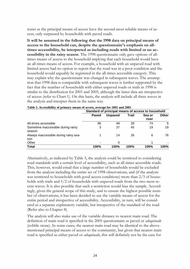
24
water as the principal means of access have the second most reliable means of ac-cess, only surpassed by households with paved roads.
It will be assumed in the following that the 1998 data on principal means of access to the household can, despite the questionnaire's emphasis on all-times accessibility, be interpreted as including roads with limited or no ac-cessibility in the rainy season. The 1998 questionnaire only gave options of all-times means of access to the household implying that each household would have an all-times means of access. For example, a household with an unpaved road with limited access had no option to report that the road was in a poor condition and the household would arguably be registered in the all-times accessible category. This may explain why the questionnaire was changed in subsequent waves. The assump-tion that 1998 data is comparable with subsequent waves is further supported by the fact that the number of households with either unpaved roads or trails in 1998 is similar to the distribution for 2001 and 2005, although the latter data are irrespective of access (refer to Chart 1). On this basis, the analysis will include all three waves in the analysis and interpret them in the same way.
Table 5. Accessibility of primary means of access, average for 2001 and 2005
Standard of principal means of access to household
Paved Unpaved Trail Sea or river
Other
All-times accessible 96 49 28 74 5
Sometime inaccessible during rainy season
3 37 45 19 19
Always inaccessible during rainy sea-son
1 14 26 6 76
Other - 0 1 -
Total 100% 100% 100% 100% 100%
Alternatively, as indicated by Table 5, the analysis could be restricted to considering road standards with a certain level of accessibility, such as all-times accessible roads. This, however, would entail that a large number of households would be excluded from the analysis including the entire set of 1998 observations, and (if the analysis was restricted to households with good access conditions) more than 2/3 of house-holds with trails and 1/2 of households with unpaved roads from the two most re-cent waves. It is also possible that such a restriction would bias the sample. Accord-ingly, given the general scope of this study, and to ensure the highest possible num-ber of observations, it has been decided to use the variable means of access for the entire period and irrespective of accessibility. Accessibility, in turn, will be consid-ered as a separate explanatory variable, but irrespective of the standard of the road (Refer also to Chapter 8).
The analysis will also make use of the variable distance to nearest main road. The definition of main road is specified in the 2005 questionnaire as paved or adoquinado (cobble stone). In some cases, the nearest main road may be identical to the above-mentioned principal means of access to the community, but given that nearest main road is specified as either paved or adoquinado, this will definitely not be the case for

25
households who have indicated their principal means of access to be unpaved, sea/river or trail.
The proportion of households living more than 50 km away from the nearest main road has more or less remained stable from 2001 to 2005. The next rural road related variable concerns the distance to main road which is only available for 2001 and 2005. Looking at all observations for both waves, the data suggest that households living within 5 km of the nearest main road decreased from 32.6 per cent in 2001 to only 26.2 per cent in 2005. Similarly, the proportion living more than 50 km away has increased from 24.4 per cent to 35.3 per cent. However, the in-crease in the proportion of households living far away from a main road may also imply that that the sample for 2005 includes more rural households than earlier samples. This assumption is supported the results derived from restricting the com-parison to the 1,389 respondents participating in both the 2001 and 2005 waves. In this case the proportion living within 5 km of the nearest main road has been stable over time at roughly 33 per cent, while the proportion living more than 50 km away has in fact decreased, albeit slightly, from 23 per cent to 20 per cent.
The next variable to be introduced indicates whether households have benefitted from a road improvement project since the last interview. It should be noted by way of introduction that it is not clearly defined what is implied by "benefitting from a road improvement project", but it is assumed that most members of a community would answer in the affirmative if a road leading to their community had been reha-bilitated or improved since the last interview.
The proportion of rural households who has befitted from a road programme has fluctuated significantly over time, peaking in 2001 at 31.2 per cent. In 1998 the proportion was only 6.6 per cent and in 2005 20.3 per cent. The peak noted in 2002 is arguably a result of the large volume of infrastructure construction projects carried out in the aftermath of Mitch.
Table 6 below demonstrates responses to the question whether the quality of the principle means of access has changed since last interview.
The data indicate that the respondents' assessment of the condition of the rural road network has remained largely unchanged over the 1998- 2001 pe-riod. However, as Table 6 demonstrates, a 12 percentage point increase can be reg-istered for those who report to have experienced deterioration of their principal means of access since last interview. It is possible that this is a reflection of the damage done by the hurricane Mitch in 1998 immediately after the last round of interviews.

26
Table 6. Change in quality of primary means of access since last interview
Since [year of last interview], the
access to this dwelling:
1998
(n=1,834)
2001
(n=1,839)
Has improved 14% 13%
Still the same 61% 61%
Has deteriorated 12% 24%
Don't know 12% 1%
Share of households
Finally, the analysis will consider accessibility of the principle means of access, which as mentioned above is measured since 2001. It should be noted that respon-dents' assessment of road accessibility may be influenced by the means of transport available to the respondent. For example what is accessible with a four-wheel drive may not be accessible with an ordinary car, a bicycle and so forth. On the other hand a poor road may be accessible by foot but not by car and so forth. With this reservation in mind, it will be assumed that the variable can be used as a valid indi-cator of the objective level of accessibility of the road.
Assessment of road accessibility has not changed between 2001 and 2005. Table 7 shows that the proportion of respondents who face some degree of accessi-bility problems during the rainy season is stable at roughly 50 per cent. A sixth of the entire sample even report to have no accessibility at all during the rainy season. As already indicated respondents with unpaved roads and trails are much more likely to experience inaccessibility during the rainy season.
Table 7. Accessibility of primary means of access
Is the primary access to the community…
2001
(n=1,838)
2005
(n=3,250)
Accessible all year round? 48% 50%
Accessible during some of the rain
season?
35% 32%
Not accessible during the rain season? 16% 17%
Share of households
The above-mentioned variables will be used as independent variables in the follow-ing sections with a view to examining their explanatory power for a number of ef-fect and impact variables.
Direct Employment
As mention by Howe, the first and most certain effect from a rural road project is the employment generated by the construction of the road. The survey data include general information about household involvement in road construction projects.
Out of those who claim to have benefitted from a road project in 2005, 15 per cent have themselves contributed to the project, typically by providing la-bour. The proportion contributing for 1998 was 30 per cent and only 13 per cent in 2001. Accordingly, there is some measurement of community involvement in rural road projects, but the level of involvement fluctuates significantly. Among those who contribute to road projects, men and women are equally likely to do so – and

27
the contribution is predominantly through labour (other types of contributions in-clude financing and materials).
Transport
Moving focus from descriptive statistics to regressions analysis, three pooled regres-sion analyses were carried out to estimate the impact of rural road related variables on transportation. The results are presented in Table 8. The same regressions have also been carried out using the fixed effects method. The corresponding results are available in Table 9.
The first pooled regression analysis is carried out to estimate the degree to which construction of roads is accompanied by the emergence of transport services such as busses, lorries etc. Given that no EMNV data are available to directly measure the presence and nature of transport services on the road network, household spending on transport is used as a proxy indicator for the existence of transport ser-vices. The variable is measured as a dummy variable.
The proxy variable does not consider the unit cost of transport services (price of bus ticket for example) and hence assumes that households can afford these ser-vices. It is also worth noting that the concepts of taxis, public buses may quite likely be either irrelevant for or interpreted differently by respondents. For example it is possible that respondents would classify a truck that provides a ride for a small amount as a bus, a truck or a taxi - or it would simply not be reported as a transport service in which case the real supply of transport services would be underreported.
There are indications that the presence of a paved or non-paved road as the principal means of access to the household causes transport services to exist. The highly significant regression results show that households that have either paved (regression coefficient of 0.539) and also to some extent unpaved roads (coef-ficient 0.275) as their principal means of access are more likely to pay for transport services than households with trails as their main access. These results are, however, not backed up by the fixed effects regression.
Having benefitted from a rural road project appears to make households in-cur expenditure for transport services. The results of the pooled regression analysis have produced a highly significant (1 per cent level) coefficient to indicate that those who benefit from road projects spend money on transport services - thus suggesting that transport services emerge where road projects have been carried out. A similar result emerges from the fixed effect regression analysis at a 1 per cent con-fidence level. The emergence of transportation services is, as mentioned, important for the wider benefits of rural roads to appear.
The next transportation related variable concerns travel time to health facilities and schools. The data reports travel time using public transportation (including waiting time) and it is assumed that the data reflects average transportation time.
There are indications that households with either paved or non-paved roads have a lower travel time to service delivery units. The pooled regression analyses consider to what extent travel time to respectively health facilities and schools is a

28
result of the standard of means of access to the household. The regression coeffi-cients confirm at a very high level of confidence (1 per cent) that travel time is re-duced for households with paved roads and unpaved roads compared to households with trails. Moreover, judging by the value of the regression coefficient, the reduc-tion in travel time appears to be stronger in the case of households with paved roads (-0.726 for travel time to health clinics) than for households with unpaved roads (-0.405). However, the coefficients returned by the fixed effects regression model are insignificant. This, as mentioned does not imply that the causal relationship can be ruled out but the causal relationship may be less certain than initially suggested by the pooled regression analysis, arguably as a result of omitted variables bias. Includ-ing information on the accessibility of the route to the service delivery unit would arguably further strengthen the explanatory power of the analysis.
Households that have benefitted from a road project also tend to have lower travel times: Results from the pooled regression analysis show that travel time to both schools and health clinics is significantly lower for households that have bene-fitted from a road project. The results are backed up by the result of the fixed re-gression model with respect to travel time to health facilities, but not for travel time to schools.
Households that have experienced deterioration in the quality of their princi-pal means of access tend to experience a longer travel time to schools and health facilities. The data returned by the pooled regression model suggest that the quality of the road has a bearing on household access to service delivery units, at least when the quality of the road has become worse. This, however, is not con-firmed by the fixed effects analysis. The fixed effects analysis does, however, sup-port the notion that households that experience an improvement in the road situa-tion will have shorter travel time to health clinics. It should be noted that the regres-sion results related to change in the road conditions, available in Appendices 2 (pooled) and 3 (fixed effects), only cover the period 1998-2001.
The importance of the condition of the road for travel times is also indicated by using accessibility of the principal means of access as an explanatory vari-able. The results from the pooled regression, only available for 2001-2005, suggest (at the 1 per cent level of confidence) that households which rate their roads as "sometimes inaccessible" during the rainy season, or even "always" inaccessible dur-ing the rainy season, have a longer travel time to schools as well as to health clinics (results available in Appendix 4). The results are confirmed by the fixed effects analysis (available in Appendix 5) with respect to households who have only partial access during the rainy season (coefficient with 1 per cent level of confidence for travel time to health clinics and coefficient with 5 per cent level of confidence for travel time to schools).
Agriculture
Given the dominance of agriculture in rural Nicaragua, rural roads would be ex-pected to have a significant impact on the livelihoods of farmers through changes in input and output prices. Three pooled regression analyses have been carried out

29
considering effect for farmers marketing crops. They have also been carried out us-ing the fixed effects model.
The means of access to a household does not have any significant bearing on whether households receive agricultural extension services or in general buy agricultural inputs. The lack of association is confirmed by the fixed effects model. A qualitative analysis looking at the various types of agricultural inputs and extension services and the context in which they are delivered may be able to inform more sophisticated model estimation for this variable. Both variables are measured as dichotomous dummy variables. Thus the analysis considers whether or not farm-ers receive inputs but does not capture whether farmers who already receive some measure of inputs and extension services increase/decrease their input as a result of rural road related changes.
Similarly, there is no clear association between accessibility and agricultural output. Moving focus to the output side, by examining the total value of the agri-cultural sale, the regression analysis finds only limited significant results. Focusing on the period 2001-2005, the pooled regression analysis finds that households that characterise their principal means of access as either partly or never accessible dur-ing the rainy season have a significantly lower agricultural output. The regression coefficients (available in Appendix 4) are, however, only at the 10 per cent level of significance and are not supported by the fixed effects analysis. Moreover the cau-sality may run both ways: Farmers with high outputs may be in a better position to relocate to areas with good access, or they may be able to choose means of trans-port that can overcome bad road conditions. They may therefore not rate the objec-tive condition of the road in the same way as a farmer with a weaker type of trans-portation.
Non-Farm Employment
Household income from non-agricultural activities appears to be positively influenced by the rural road indicators. The theoretical analysis pointed out that the emergence of an improved rural road network would have positive implications for diversification of the economy. To probe this, a pooled multivariate regression analysis was carried out to explain salary derived from non-agricultural activities. All of the rural roads coefficients have a significant bearing on non-agricultural income. Households with paved and unpaved roads are far more likely to have non-agricultural income than those with trails as their mean access. Similarly, the regres-sion coefficient for distance to main road is negative and highly significant suggest-ing that households located far away from a main road will, all others thing being equal, be less likely to take up non-farm activities. The data is only available for 2005 so no fixed effects regression analysis has been carried out.

30
Table 8. Pooled Regression, 1998 - 2005 Model no. (1,1) (1,2) (1,3) (1,4) (1,5) (1,6) (1,7) (1.8a) (1,9) (1,10)
Type Logistic Pooled OLS Pooled OLS Logistic Logistic Pooled OLS Pooled OLS Pooled OLS Logistic Logistic
Dependent variable dcons_transport log(transtime_health) log(transtime_school) dtechassist1
dbuy_agri_input log(sale_agri) log(salary_nonagri) log(consumption) ddisease dilliterat
Waves included 1998-2005 1998-2005 1998-2005 1998-20052
1998-20052
1998-20052
2005 1998-2005 1998-2005 1998-2005
No. of observations 7.003 6.989 6.989 3.614 3.614 3.614 3.240 7.005 7.005 6.956
R-squared 0,171 0,199 0,110 0,152 0,190 0,163 0,233 0,092 0,498
Explanatory variables:
Intercept -3,001 *** 4,345 *** 3,426 *** -2,450 *** 1,265 *** 7,422 *** 0,317 8,932 *** -1,274 *** -0,888 **
dpaved 0,539 *** -0,726 *** -0,202 *** 0,235 -0,132 -0,048 0,476 ** 0,188 *** -0,224 * -0,451 ***
dunpaved 0,275 *** -0,405 *** -0,203 *** 0,220 -0,122 0,024 0,408 *** 0,082 *** -0,267 *** -0,168 **
dsea_river -0,166 -0,284 *** -0,444 *** -1,003 * -0,805 *** 0,144 0,578 * 0,160 *** -0,415 ** -0,619 ***
dother_transport -0,880 *** 0,321 *** 0,313 *** -0,638 -0,268 -0,077 0,032 -0,096 ** 0,604 ** 0,802 ***
dbene_road 0,428 *** -0,107 *** -0,079 ** 0,074 0,119 0,046 0,063 0,103 *** -0,254 *** -0,054
droad_qual_imp
droad_qual_det
logdist_mainroad -0,240 ***
daccessible_rain_some -0,291 **
daccessible_rain_never -0,356 **
dbene_other 0,261 *** -0,273 *** -0,335 *** 0,171 0,189 * -0,041 0,651 *** -0,045 *** 0,505 *** -0,019
dependent_ratio -0,687 *** 0,164 *** 0,054 -0,246 -0,562 *** -0,257 ** -1,370 *** -0,706 *** 1,080 *** 1,324 ***
age_hhhead 0,057 *** 0,001 -0,004 0,041 * -0,001 0,044 *** 0,036 * -0,019 *** 0,062 *** 0,117 ***
age_hhhead_sq 0,000 *** 0,000 0,000 0,000 0,000 0,000 *** 0,000 0,000 *** 0,000 *** -0,001 ***
dfemale_hhhead -0,075 -0,172 *** -0,130 *** -0,591 *** -0,345 *** -0,581 *** 0,238 * -0,029 * -0,085 -0,376 ***
dedu_elementary 0,306 *** -0,219 *** -0,181 *** 0,527 *** 0,210 ** 0,176 *** 0,672 *** 0,202 *** -0,055 -3,183 ***
dedu_secondary 0,644 *** -0,501 *** -0,292 *** 0,669 ** 0,257 0,197 2,562 *** 0,468 *** -0,155 -4,158 ***
dedu_higher 0,705 *** -0,751 *** -0,525 *** 1,886 *** -0,173 1,171 *** 4,274 *** 0,976 *** -0,607 *** -5,079 ***
dagri_problems
d2001 0,377 *** 0,056 -0,005 -0,247 0,355 *** 0,190 *** -0,011 0,239 ** 1,036 ***
d2005 0,179 *** 0,091 *** -0,066 ** -1,147 *** 1,030 *** 0,542 *** 0,047 *** 0,418 *** 0,790 ***
dmitch2001 -0,213 -0,106 -0,005 0,440 -0,313 -0,269 ** -0,059 -0,255 0,231
dmitch2005 -0,186 -0,117 * -0,081 -0,228 -0,183 -0,165 -0,053 -0,115 *** 0,107 -0,097
Department dummies *** *** *** *** *** *** *** *** *** *** Note: * indicates parameter estimates significantly different from zero at the 10 per cent level, ** at the 5 per cent level, and *** at the 1 per cent level

31
Table 9. Fixed Effects Regression, 1998 - 2005
Model no. (2.1) (2.2) (2.3) (2.4) (2.5) (2.6) (2.7) (2.8) (2.9) (2.10)
Type Conditional logistic Fixed effects Fixed effects Conditional logistic Conditional logistic Fixed effects Fixed effects Conditional logistic Conditional logistic
Dependent variable dcons_transport log(transtime_health) log(transtime_school) dtechassist1
dbuy_agri_input log(sale_agri) log(consumption) ddisease dilliterat
Waves included 1998-2005 1998-2005 1998-2005 1998-20052
1998-20052
1998-20052
1998-2005 1998-2005 1998-2005
No. of observations 4,252 4,223 4,225 2,184 2,185 2,184 4,234 4,252
R-squared3
0.073 0.757 0.714 0.247 0.212 0.672 0.754 0.067 0.306
Explanatory variables:
Intercept 3.963 *** 3.826 *** 5.775 *** 8.819 ***
dpaved -0.031 -0.046 0.001 0.085 0.014 0.102 0.004 -0.605 ** -0.158
dunpaved 0.070 0.025 0.016 0.178 -0.378 0.041 0.005 -0.132 0.089
dsea_river -0.011 0.019 0.202 -14.840 0.675 0.066 -0.038 -1.817 ** -0.020
dother_transport 0.225 0.047 0.420 *** 16.409 1.088 -0.024 0.095 1.259 * 0.283
dbene_road 0.414 *** -0.068 * -0.007 -0.009 -0.137 -0.025 0.106 *** -0.370 ** 0.095
droad_qual_imp
droad_qual_det
logdist_mainroad
daccess_most
daccess_never
dbene_other 0.317 *** -0.050 -0.010 0.131 0.313 0.063 -0.032 0.271 * -0.145
dependent_ratio -0.220 -0.017 0.063 0.599 -0.451 -0.389 * -0.285 *** 0.544 0.669
age_hhhead 0.023 0.014 -0.004 -0.120 -0.123 * 0.067 *** -0.010 * 0.009 0.085 *
age_hhhead_sq 0.000 -0.0002 * 0.000 0.001 0.001 * 0.000 * 0.000 ** 0.000 -0.001 **
dfemale_hhhead -0.359 -0.016 0.020 0.233 -1.103 * -0.075 0.031 -0.029 -1.052 ***
dedu_elementary -0.090 0.008 -0.047 -0.163 -0.192 -0.020 0.040 -0.099 -2.517 ***
dedu_secondary -0.011 -0.067 -0.011 -1.259 -0.924 0.189 0.206 *** -0.142 -3.218 ***
dedu_higher -0.522 -0.198 -0.140 15.420 -1.022 0.141 0.399 *** -0.380 -4.361 ***
dagri_problems
d2001 0.711 *** -0.084 ** -0.037 -0.293 0.356 * 0.047 0.007 0.402 *** 1.778
d2005 0.331 *** -0.103 *** -0.132 *** -1.254 *** 1.680 *** 0.522 *** 0.069 *** 0.845 1.305 ***
dmitch2001 -0.465 ** -0.043 0.005 0.667 -0.637 -0.040 0.002 -0.155 -0.081
dmitch2005 -0.264 -0.064 -0.017 0.022 -0.876 * 0.109 -0.013 0.073 -0.337
Cross-sectional effects - *** *** - - *** *** *** ***
1: In the 2005 questionnaire the different types of tech.assistance is not listed (in contrast to 1998 and 2001). This may cause the "yes"-rate to drop
2: Only farmers included in the regression.
3: The R-squared values of the conditional logistic and fixed effects models are not comparable.
N.a - only 1
cross-section
log(salary_non
agri)
Note: * indicates parameter estimates significantly different from zero at the 10 per cent level, ** at the 5 per cent level, and *** at the 1 per cent level

32
Consumption
In the following attention is devoted to examining the power of rural roads access as an explanatory variable for household welfare. Consumption, which includes value of consumption of own agricultural outputs and imputed rent, is used as the main welfare indicator in the study. The results of the various consumption-related regression analyses are presented below.
There is a clear association between the primary means of access to the household and median consumption levels. Households having paved road as the primary means of access earn well above households with other types of access as documented by Table 10 below. This pattern applies to all of the three waves under analysis.
Table 10. Median consumption vs. primary access to dwelling. Cordobas, 2005-prices
Wave
Primary road type 1998 2001 2005
Paved street 6,437 7,769 6,798
Unpaved street 5,744 5,743 5,684
Trail 4,652 4,823 5,274
Sea or river 5,172 5,762 6,103
Other 4,167 - 4,680
The positive consumption impact of the standard of the household means of access is confirmed by the pooled regression analysis. The results of the pooled regression analysis in Table 8 show that households with paved roads and unpaved roads have a significantly higher consumption than households with trails only. This result is however not backed up by the fixed effects model.
Interestingly households with sea or river as the main access also have a significantly higher consumption than households with trail only. The result could potentially be explained by the fishery economy and way of life in RAAS and RAAN where households with sea or river access are typically located. Besides, as already docu-mented by Table 5, almost 75 per cent of households with sea or river access have all-year accessibility - a proportion only second to households with paved roads. Qualitative analysis would arguably be required to further examine this.
Households that have benefitted from a rural road project also tend to have a higher consumption. As demonstrated by Table 11 below, which applies a differ-ence-in-difference approach, there is a well documented positive consumption ef-fect from having benefitted from road projects: Those who have benefitted have experienced a 10 per cent increase in their (median) consumption over the period 2001-2005 while those not benefitting have had a consumption increase of only 1 per cent. The positive association between consumption and road projects is also confirmed by the pooled regression analysis and the fixed models regression, which returns a positive regression coefficient at the 1 per cent level.

33
Table 11. Beneficiary of road improvements vs. change in median consumption, Cordobas, 2005-
prices
Last interview This interview
No (n = 1,878) 5,370 5,447 1%
Yes (n = 753) 5,571 6,132 10%
Beneficiary of road improvement
program since last interview?
Median consumption Percent
change
Note: Only 2001- and 2005 waves (no information on "last interview" consumption for 1998). Only households that have participated in two consecutive waves. The picture is the same when 2001 and 2005 are treated separately.
The consumption impact of an improved road condition is somewhat am-biguous: For the 1998-2001 waves, the pooled regression analysis has also consid-ered the impact of improvements in the road condition (refer to Appendices 2 and 3). While a positive and very significant impact on consumption can be noted in households where the condition of the primary means of access has improved, this result is not backed up by the fixed effects analysis. Hence the association can only be said to be indicative and it is possible that including other variables such as a proxy for household wealth would further strengthen the analysis.
Distance to main road and consumption are associated. As demonstrated in Table 12 below those living within 1 km of a main road have a median income that is well above those living between 1 and 5 km from the nearest main road. Those living more than 25 km away from a main road earn roughly 2/3 of those living within 1 km of a main road.
Table 12. Distance to main road vs. change in median consumption, Cordobas, 2005-prices
No. of households Median consumption
Distance to main road 2001 2005 2001 2005
Less than 1 km 289 480 7,663 7,544
1-5 km 310 402 6,650 6,414
5-25 km 567 877 5,192 5,595
25-50 km 223 422 5,170 5,043
More than 50 km 450 1,189 5,308 5,281
A general positive association between distance to main road and household consumption is confirmed by the regression analysis: The pooled regression analysis has considered data for the period 2001-2005 only (no data available for 1998, results available in Appendix 4). The impact of distance to main road on household consumption is positive and highly significant. This result is also con-firmed by the fixed effects analysis (Appendix 5).
Finally, household consumption appears to be negatively affected for house-holds where the principal means of access is only accessible part of the rainy season. The pooled regression analysis has considered, for the waves 2001-2005, whether all-time accessibility of the roads (an indication of the condition of the road) has a bearing on consumption levels and finds that limited access during the rainy season impacts negatively on consumption at the 1 per cent confidence level. Surprisingly, the consumption impact is less negative for households whose means of access is never passable during the rainy season. It is possible that this type of household has adapted to the difficult access situation by organising agricultural
34
activities differently - for example by relying mainly on locally available inputs and markets.
Distributional Effects
As pointed out in the theoretical analysis (Chapter 3), the positive welfare effects from rural road investments may not benefit all income groups to the same extent. The study has considered whether the general positive impacts on consumption apply irrespectively of income (measured as poverty status of the household at time of last interview) and gender (measured as the sex of the household head). The re-sults using pooled regression analysis are presented in Table 13 below.
The extreme poor do not appear to derive the same magnitude of benefits from rural roads as groups with a higher income. The analysis shows that the general and highly significant impact on consumption (0.14) of having a paved road as the main means of access is neutralised in the case of the extreme poor (-0.16) again at a relatively high level of confidence (5 per cent). When the analysis is re-stricted to the non-extreme poor (i.e. those whose income is above the extreme poverty line, but below the poverty line) no significant impact is found. Accordingly, while rural roads investments appear to have a direct and positive impact on the welfare of the poor, this does not apply to the poorest of the poorest. This is in line with the theoretical analysis in which it was suggested that the benefits derived from rural roads may not always apply to the poorest groups in the short run – typically because the poorest lack basic resources to take advantage of new opportunities brought about by rural roads, such as an increased supply of transportation services. However, some caution is warranted given that the results are not confirmed by the results of the fixed effects analysis.

35
Table 13. Distributional Effects, Pooled Regression Results Model no. (3,1) (3,2) (3,3)
Type Pooled OLS Pooled OLS Pooled OLS
Dependent variable log(consumption) log(consumption) log(consumption)
Interaction variable1
lag(dpoor_extreme) lag(dpoor) dfemale_hhead
Waves included 2001-2005 2001-2005 1998-2005
No. of observations 2.625 2.625 7.005
R-squared 0,332 0,350 0,234
Explanatory variables
Intercept 8,92 *** 9,20 *** 8,95 ***
dpaved 0,14 *** 0,14 *** 0,16 ***
dunpaved 0,03 0,02 0,07 ***
dsea_river 0,01 0,00 0,15 ***
dother_transport -0,15 -0,51 ** -0,08 *
dbene_road 0,11 *** 0,12 *** 0,09 ***
interaction var. -0,46 *** -0,47 ***
dpaved * interaction var. -0,16 ** -0,06 0,15 ***
dunpaved * interaction var. -0,02 0,02 0,07 *
dsea_river * interaction var. 0,09 0,07 0,07
dothertrans * interaction var. 0,00 0,78 ** -0,07
dbene_road * interaction var. 0,08 0,02 0,07
dbene_other -0,09 *** -0,06 ** -0,04 ***
dependent_ratio -0,48 *** -0,48 *** -0,71 ***
age_hhhead -0,01 *** -0,02 *** -0,02 ***
age_hhhead_sq 0,00 *** 0,00 *** 0,00 ***
dfemale_hhhead 0,03 0,04 -0,10 ***
dedu_elementary 0,14 *** 0,12 *** 0,20 ***
dedu_secondary 0,36 *** 0,31 *** 0,47 ***
dedu_higher 0,80 *** 0,72 *** 0,98 ***
d2001 -0,01
d2005 0,04 * 0,04 * 0,05 ***
dmitch2001 -0,06
dmitch2005 -0,04 -0,03 -0,12 ***
Department dummies *** *** *** Note: * indicates parameter estimates significantly different from zero at the 10 per cent level, ** at the 5 per cent level, and *** at the 1 per cent level
The general positive impact of having a paved road as the principal means of access appears to increase in the case of households with a female head. The pooled regression analysis in Table 13 demonstrates how the interaction between gender and rural roads impacts on household consumption. The analysis considers the gender of the household head as a general proxy indicator for gender and finds a very significant (1 per cent) interaction effect. Accordingly, the positive consump-tion impact derived from having a paved road as the principal means of access ap-pear to be stronger in the case of households headed by women. The coefficients returned by the fixed effects analysis (see Table 14 below) do, however, not support this. Here part of the explanation may be low number of observations: Only few households may have experienced a change in the gender of the household head in the course of the period under analysis.
The association suggested by the pooled regression analysis could possibly be ex-plained by the existence of improved rural roads which gives women the possibility of travelling to and from the household more frequently thus making it possible to combine work outside the households with domestic duties. Alternatively, the im-

36
proved access to the household may enable female entrepreneurs working from home to more easily acquire inputs and market their produce.
Table 14. Distributional Effects, Fixed Effects Regression Results Model no. (4,1) (4,2) (4,3)
Type Fixed effects Fixed effects Fixed effects
Dependent variable log(consumption) log(consumption) log(consumption)
Interaction variable lag(dpoor_extreme) lag(dpoor) dfemale_hhead
Waves included 2001-2005 2001-2005 1998-2005
No. of observations 2.365 2.365 4.229
R-squared 0,860 0,869 0,754
Explanatory variables
Intercept 8,977 *** 8,630 *** 8,823 ***
dpaved -0,022 0,048 -0,009
dunpaved -0,007 -0,010 -0,009
dsea_river -0,171 -0,125 -0,030
dother_transport -0,088 0,054 0,120
dbene_road 0,131 *** 0,214 *** 0,095 ***
interaction var. 0,284 *** 0,391 ***
dpaved * interaction var. -0,017 -0,110 0,073
dunpaved * interaction var. 0,002 0,011 0,084
dsea_river * interaction var. 0,010 -0,089 -0,030
dothertrans * interaction var. 0,000 -0,089 -0,189
dbene_road * interaction var. -0,092 -0,149 *** 0,048
dbene_other -0,040 -0,054 * -0,031
dependent_ratio -0,242 *** -0,217 *** -0,287 ***
age_hhhead -0,006 -0,002 -0,010 *
age_hhhead_sq 0,000 0,000 0,000 **
dfemale_hhhead 0,043 0,062 -0,029
dedu_elementary -0,016 -0,032 0,040
dedu_secondary 0,064 0,063 0,207 ***
dedu_higher 0,182 0,163 0,400 ***
d2001 0,103 *** 0,117 *** 0,005
d2005 0,065 ***
dmitch2001 0,035 0,053 0,006
dmitch2005 -0,010
Cross-sectional dummies *** *** *** Note: * indicates parameter estimates significantly different from zero at the 10 per cent level, ** at the 5 per cent level, and *** at the 1 per cent level
Social Development
Just as rural roads are generally assumed to increase general welfare, as measured by consumption in the section above, they are also believed to translate into improved social development impacts for the population in the road influence area – partly as a result of the earlier demonstrated reduction in travel time. Below the results of pooled and fixed effects regression analyses considering health and education are presented (refer also to Tables 8 and 9).
The prevalence of sickness (any type save diarrhoea) during the past month has been included as a proxy indicator for the health status of the household. It is ar-guably a long term impact of rural road improvement, but the variable captures all kinds of diseases and is therefore relevant to use on a national basis. Some of the more short term based variables on treatment are specific to certain diseases and their prevalence across the country may vary due to many factors not related to rural

37
roads.
Households with paved or unpaved roads are, according to the pooled re-gression analysis, less likely to fall sick than households with trail as the principal means of access. Similarly, households that have benefitted from a road projects are, also according to the pooled regression analysis, less likely to report sick. This finding is also confirmed by the regression results for the period 2001-2005 only (refer to Appendix 3) which demonstrate that households that have either limited or total lack of access during the rainy season are more likely to have re-ported sick in the previous month. Although not confirmed by the fixed effects re-gression (refer to Appendix 4) this finding corresponds well with the previous find-ing that limited access also implies a significant increase in travel time to health clin-ics. To corroborate the findings, it is worth noting that the fixed effects regression analysis also finds that having a paved road, or being a beneficiary of a road project, significantly reduces the likelihood that households have reported sick in the previ-ous month. Similarly the fixed effects analysis considering 2001-2005 (results in Ap-pendix 5) shows that distance to main roads is an important parameter for explain-ing propensity to fall sick. The further away a household is located, the more likely is it that one of its members has called sick in the previous month. Finally, it is worth noting that the improved health situation observed for households with paved roads as their principal means of access may also be a result of increased con-sumption levels, which generally have a positive impact on health outcomes.
Literacy levels are included in the analysis to test for the impact of rural roads on education. The variable is measured as a dummy, and tracks if at least one of the household's members between the age of 15 and 64 is able to both read and write. Again this is arguably a long term impact of rural roads but it has the advantage of being generic and comprehensive in comparison to attendance variables by tracking the quality and impact of school attendance.
Finally, the pooled regression model suggests that rural road access has a positive impact on literacy levels. This suggests that the shorter travel time to schools registered for households with paved and non-paved roads, may in fact translate into improved learning outcomes – even when controlling for level of edu-cation of the household head. The coefficients are highly significant for households with paved and non-paved roads as their main means of access. The fixed effects model does, however, not find significant results to back this up. On the other hand, pooled regression results for the period 2001-2005 (refer to Appendix 4) very clearly indicate that households whose access is limited during the rainy season, ex-perience a significantly higher illiteracy rate compared to households with no access problems. Again this cannot be confirmed by the fixed effects regression analysis (refer to Appendix 5) which suggests that the association is less certain than indi-cated by the pooled regression analysis.
Given the long term nature of both the health and education related variables, the impact on both health and education may be clearer once a longer period of data is available for analysis.

38
7. Conclusions
Nicaragua will need to increase economic growth rates to make further progress in combating poverty, especially in the rural areas, where the incidence of poverty is far greater than in urban areas. At the same time, Nicaragua's endowment of rural roads is in a fairly poor condition compared to its neighbours, especially with respect to the condition of the tertiary network. There are indications that the relatively poor state of the rural infrastructure is part of the reason why poverty rates have only been reduced marginally.
This study provides some evidence that rural roads play a role in improving welfare in rural areas in Nicaragua. The finding is mainly confirmed by the pooled regression analysis: Where roads have improved, welfare tends to follow; where roads have deteriorated, the rural communities do less well. However, the results are far from conclusive, especially when restricting the analysis to fixed ef-fects analysis. However, as already pointed out, the lack of a significant relationship in the fixed effects models is not sufficient to rule out the causal relationship sug-gested by the pooled regression analysis due to the weaknesses of the fixed effects models described in Chapter 5. It does however suggest that the relationships are less certain than what the pooled regression analysis otherwise suggests and there is clearly a case for further strengthening the analysis by bringing in more variables to address the so-called omitted variables bias (see next Chapter). The below conclu-sions should be read in that light:
The results suggest that poor households (except extreme poor) who benefit from road projects tend to spend money on buses, lorries etc. Hence, despite the existence of a limited and relatively old vehicle park, there are indications that transport operators do set up business in areas where roads permit. This finding is crucial given that transportation services are the precondition for all of the subse-quent impacts to emerge – irrespective of whether people travel themselves or bene-fit from an increased influx of goods and services. The results also indicate a posi-tive impact of rural roads on travel times. For example, beneficiaries of road pro-jects tend to have significantly shorter travel times to service delivery units, a finding that was confirmed by both types of regression analysis (pooled and fixed).
Unlike results from Bangladesh and India, there is only limited evidence to support the notion that rural roads impact on agriculture. There is no clear impact of rural road variables on propensity to make use of agricultural inputs. This suggests that there are other, more important factors at play in determining agricul-tural inputs and outputs. This could be land endowments, other factors related to economic development potential of a given area, competitiveness of markets, and impacts from exogenous shocks such as the 2002 coffee crisis.

39
On the other hand, as suggested by studies from other countries, there are indications that distance of a household to a main road has implications for diversification of the economy. Using salaries derived from non-farm activities as a proxy, the pooled regression analyses find significant results. The closer a house-hold is located to a main road, the more likely is it to be engaged in non-farm activi-ties. This is an interesting finding suggesting that rural roads may indeed play a criti-cal role in creating alternative employment opportunities in rural Nicaragua. How-ever, these results are based only on pooled regression analysis of 2005 data and clearer results may materialise once more data becomes available.
The study finds that rural roads access has some influence on household consumption. This finding is confirmed for all of the rural road related variables included in the pooled regression analyses and provides some evidence that rural roads play a role in stimulating growth in rural Nicaragua. The results returned by the fixed effect model are less clear. A significant consumption effect can only be determined by the fixed effects model with respect to households that have benefit-ted from a road project.
The consumption impact identified through the pooled regression analysis does not appear to be equally shared by all income groups. The results from the pooled regression analysis indicate that the non-extreme poor more or less de-rive the same benefits as the rural population in general, but the positive impact is neutralised when the analysis is restricted to the extreme poor – arguably because a minimum level of skills and resources are required to take advantage of the benefits provided by a change in the rural road situation.
The chain of events through which rural road access may impact consump-tion is not clear. As reported the results for agricultural activities are inconclusive and several of the results returned by the fixed effects model are also insignificant. The overall consumption effects documented by the pooled regression analysis could instead be a reflection of a wider set of variables related to the economic de-velopment potential of a given area and social development outcomes.
The latter argument is supported by the fact that rural roads appear to have an impact on especially health outcomes: The pooled regression analysis has considered impact on literacy and the tendency of the households to report sick. In both cases rural roads access appears to have an impact. The result for health out-comes is also supported by the fixed effects analysis, while no clear result was re-turned for literacy. The observed impact is arguably a result of improved access conditions. As mentioned rural roads access is believed to explain changes in travel times to social service delivery units.
Finally, returning to the caveats listed at the beginning of this study, it should be noted that risks of endogeneity are ever present. For example, a vari-able like "having a paved road leading to the community" has been found to have an impact on travel times, health outcomes and other impact variables in the pooled models. This in turn may suggest that these changes have been brought about by the road standard. It may however also reflect that paved roads tend to be established in

40
areas that are relatively well off in terms of consumption, and consequently health outcomes; in particular since the fixed effects models (which account for unob-served characteristics) did not confirm the results. Accordingly, to further corrobo-rate the conclusions, suggestions are made in the following Chapter for further stud-ies and analysis.

41
8. Further Studies
The basis for rigorously determining the impact of rural roads in Nicaragua for the period 1998-2005 can be further strengthened through a number of ways:
Expand the number of variables to be included in the analysis to reduce the omitted variables bias. The EMNV data includes a substantial number of vari-ables, including several that could further strengthen the analysis if the scope enlarged. These include:
• Additional control variables such as distance to service delivery units;
• The questionnaire asks a number of questions in the area of agricultural activi-ties such as the condition of the route used to market crops;
• Short-term based variables on health and education and related control variables such as health insurance, prevalence of vaccinations etc.;
• Similarly, the study poses a number of questions to explore respondents' rea-sons for not attending health clinics and schools. Transportation related vari-ables are among the possible causes and it may add value to include such infor-mation in the analysis.
Determine scope for and possibly use the EMNV data to construct additional variables. A case in point is the variable non-agricultural employment, which is available for 2005 only. The variable could possibly also be constructed for previous waves by drawing on a combination of variables. Likewise, it may, from the existing data, be possible to construct a measure for household wealth and an indicator to better take into account the agricultural development potential of a given household.
Moreover, important insights could possibly be gathered by running separate regression analyses for the 2001 and 2005 waves with a view to following the effects of road accessibility. It could, for example, be interesting to follow agricul-tural input and output variables for households with unpaved roads only, using ac-cessibility of the paved road as an explanatory variable for input and output. An-other way forward, given the vast differences between the various departments of Nicaragua (especially the East-West divide), could be to run separate regression analyses by departments to explore impacts more in depth.
Examine scope for including non-EMNV data in the analysis. The present study has relied on survey data related to rural roads. The results of the regression analyses would arguably improve if more precise data on rural roads could be ob-tained from other sources and paired with the household data at the lowest possible level. It would be particularly useful to include data at department or (preferably)
42
municipal level on effective road density (length of roads in good/ fair condition per 1,000 households). The findings of the Danida commissioned study "Evaluating the impact of rural roads in Nicaragua" should be considered in this context (Danida, 2007). If available, data on the economic development potential of a given area, such as population density, could also be included as an important explanatory variable.
Conduct qualitative analyses to validate some of the interpretations already offered and identify additional variables that could be included in the regres-sion analysis. It would, for example, be an opportunity to investigate the possible reasons behind some of the more unexpected results – such as the relatively weak impact on agricultural factors, and the determinants for agricultural outputs for households with sea or river as their principal means of access.
Apply more advanced statistical models to increase the econometrical reli-ability. As an example, a sophisticated modelling of time dependency in the error terms could be developed to account for possible auto-correlation. It would also be possible to further investigate possible sources of selection bias and consider reme-dial measures, such as applying the Heckman correction. Another possibility is to consider to include additional interaction effects to investigate if the relationships differ between, for instance, the East-West divide.
For future impacts assessments, the ideal set-up would be to systematically collect baseline data for target and control groups to enable difference-in-difference analysis. The support provided by development partners will presuma-bly finance the road sector in general. Accordingly, development partners may in collaboration with Government of Nicaragua develop the capacity of the Govern-ment to conduct impact evaluation analyses using target and control groups. It would arguably also be useful to further support the general M&E capacity of the Government in the rural roads sector. Factors to consider include the institutional set-up of the responsible unit, the data sources available, and the methods used for data collection. A thorough preparatory study along the lines described by COWI and RuralNet Associates (2006a & b) for Zambia could be used as a source of inspi-ration. Finally, it is considered advisable to continue using EMNV data as new waves become available. Including more data can only strengthen the basis for arriv-ing at conclusions on the causality of rural roads.

43
9. References
Allison, Paul D. (2006) Fixed Effects Regression Methods in SAS. SAS SUGI paper 184-31.
BICU, URACCAN and CIDCA/UCA (2000) Danida Transport Sector Programme Sup-port for the Autonomous Regions of Nicaragua - Broad Impact Study, Bluefields Indian and Caribbean University (BICU), Universidad de las Regiones Autonomas de la Costa Caribe Nicaraguense (URACCAN), and Centro de Investigaciones y Docu-mentacion de la Costa Atlantica.
Chatterjee, Shiladitya, Tyrell Duncan, Colandavelu Narayanasuwami, and Brahm Prakash (2004) Scaling-Up Poverty Reduction, POVERTY AND SOCIAL DEVEL-OPMENT PAPERS No. 10 / September 2004, Manila: Asian Development Bank, Regional and Sustainable Development Department.
COWI and RuralNet Associates (2006a) Poverty Impact Assessment and Baseline Study for the Road Sector - Volume 1 Main Report. Final Report prepared for the Ministry of Communications and Transport.
COWI and RuralNet Associates (2006b) Poverty Impact Assessment and Baseline Study for the Road Sector - Volume II: BaselineReport for Eastern, Northern and Western Provinces. Fi-nal Report prepared for the Ministry of Communications and Transport.
Danida (2004a) Transport Sector Programme Support (PAST) Phase 2 - 2005-2009 - Final Programme Document - Nicaragua, Copenhagen: Ministry of Foreign Affairs, Danida.
Danida (2004b) Transport Sector Programme Support (PAST) Phase 2 - 2005-2009 - Final Component Description - Component 2 - Improvement of Tertiary Transport Infrastructure in RAAN, RAAS and Region 1 - Nicaragua, Copenhagen: Ministry of Foreign Affairs, Danida.
Danida (2006) Programme Completion Report, Prepared by Gary Taylor, May 2006.
Danida (2007) "Evaluating the impact of rural roads in Nicaragua", Evaluation Study 2007/3, Prepared by Nina Blöndal, Endeleza International Development Consult-ing, Copenhagen: Ministry of Foreign Affairs, Danida.
Dercon, Stefan, Daniel O. Gilligan, John Hoddinott, and Tassew Woldehanna (2007) "The impact of roads and agricultural extension on consumption growth and poverty in fifteen Ethiopian villages" The Centre for the Study of African Economies Working Paper Series¸ Paper 260, Oxford: Centre for the Study of African Economies.

44
EIU (2007) Country Profile 2007 - Nicaragua, London: The Economist Intelligence Unit.
Howe, John (2005) Transport and Poverty Reduction, mimeo.
Johnston, Jack and John DiNardo (1997), Econometric Methods, 4th edition, McGraw-Hill, New York.
INIDE (2007) Perfil y Características de los Pobres en Nicaragua 2005, July, 2007, Mana-gua: Instituto Nacional de Información de Desarrollo.
Khandker, Shahidur R., Zaid Bakt and Gayatri B. Koolwal (2006) The Poverty Impact of Rural Roads: The Evidence from Bangladesh, World Bank Policy Research Working Paper 3875, April 2006.
NONIE (2008) NONIE Impact Evaluation Guidance, Draft prepared by Network on Impact Evaluation, subgroup2.
OECD (2000) The Glossary of Evaluation and Results Based Management (RBM) Terms, Paris: OECD.
OECD (2002) Glossary of Key Terms in Evaluation and Results-based Management, Work-ing Party on Aid Evaluation, Paris: OECD-DAC.
PAST Danida (various) Informe de Monitoreo Socioeconómico, Equipo Socioeconómico - Programa de Transporte.
United Nations (2007) Nicaragua - Valoracion Comun de Pais, Managua: Sistema de las Naciones Unidas.
van de Walle, Dominique and Dorothyjean Cratty (2002) Impact Evaluation of a Rural Road Rehabilitation Project, Washington D.C.: World Bank, January 2002.
van de Walle, Dominique (2007) Impact Evaluation of Rural Road Projects, Draft pre-pared for the World Bank PREM Sector Evaluation Notes, December 2007.
World Bank (….) Impact Evaluation - The Experience of the Independent Evaluation Group of the World Bank, prepared by Howard White, Washington D.C.: World Bank Inde-pendent Evaluation Group.
World Bank (2002) Basic Information Document, Nicaragua Living Standards Measurement Study Survey 1998, Poverty and Human Resources Development Research Group.
Wold Bank (2006) Project Appraisal Document on a Proposed Credit in the Amount of SDR 41.1 Million to the Republic of Nicaragua for the Fourth Roads Rehabilitation and Maintenance Project, May 9, 2006, Washington D.C,: World Bank.

45
World Bank (2007) World Development Report 2008 - Agriculture for Development, Wash-ington D.C.: World Bank.
World Bank (2008) The Welfare Impact of Rural Electrification: A Reassessment of the Costs and Benefits, World Bank Independent Evaluation Group (IEG), Washington, D.C.
46
Appendix 1 - Definitions of variables
Effect and impact indicators (dependent variables)
The following variables have been constructed as proxies for expected outcomes and impacts, respectively:
Transport
dcons_transport (dummy). Proxy for availability of affordable motorized transport in community. Equal to one if the household has spend money on taxis, public buses or transport ship during the past week.
transtime_health. Reported travel time from home to the nearest elementary school, measured in minutes. The logarithmic transformation has been ap-plied to reduce the sensitivity to outliers.
transtime_school. Reported travel time from home to the nearest health center or first-aid station, measured in minutes. The logarithmic transformation has been applied to reduce the sensitivity to outliers.
Agriculture
dtechassist (dummy). Equal to one if the household has received agricultural technical assistance during the past 12 months. In 1998 and 2001 the ques-tionnaire lists the different types of possible technical assistance, while this additional information was dropped in 2005. This change may have caused the yes-rate in 2005 to drop inadvertedly.
dbuy_agri_input (dummy). Equal to one if the household has spent money on agricul-tural inputs (seed, fertilizer, pesticides etc.) during the past 12 monts.
sale_agri. A proxy for the value of the farms output, measured as the total sale of cultivation in Cordobas (2005-prices, adjusted for regional price differences). The logarithmic transformation has been applied to reduce the sensitivity to outliers.
Non-farm employment
salary_nonagri. Measures the household's total earnings from non-farm employment (Cordobas, 2005-prices adjusted for regional price differences). The variable is aggregated from a number of sub-questions in the ques-tionnaire. The measure is only available for 2005.
Income / consumption
consumption. Measures the aggregate consumption per household member in Cordo-bas (2005-prices, adjusted for regional price differences). The vari-able is aggregated from a number of sub-questions in the question-naire and is available for all years. The measure comprises all types of consumption including comsumption of own agricultural pro-duction and imputed rent.

47
Health
ddisease (dummy). Proxy for household health. Equal to one if one or more of the household's members have been affected by disease (any type) dur-ing the past month.
Literacy
dilliterat (dummy). Outcome of education is measured by illiteracy. The dummy vari-able is set equal to one if at least one of the household's members between the age of 15 and 64 is not able to both read and write.
Road indicators (independent/explanatory variables)
The following 4 variables are dummy variables based in the question: What is the principal means of access to community [at all time] (paved street, unpaved street, trail, sea or river, other)? Note that in 2001, the part "at all time" was removed from the wording of the question, cf. the discussion in Chapter 6. Coded as dummies with "trail" as the ref-erence:
dpaved (dummy). Equals one if the answer is "Paved street"
dunpaved (dummy). Equals one if the answer is "Unpaved street"
dsea_river (dummy). Equals one if the answer is "Sea or river"
dother_transport (dummy). Equals one if the answer is "other"
The next 2 variables are dummy variables based on the question: Is the means of access (accessible all year, during some of the rain season, never during the rain season)? This variable is only available for 2001-2005; as the wording of the beforementioned question was changed. Coded with dummy variables with "accessible all year" as reference:
daccess_most (dummy). Equals one if the answer is "During some of the rain sea-son"
daccess_never (dummy). Equals one if the answer is "Never during the rain sea-son"
The next variable is based on the question: Since [year of last wave], is the household bene-ficiary from some program like […] construction of roads/streets (yes/no)? Note that the word-ing of the question was changed in 2001 such that construction of roads was split up in primary and local roads. Both road types have been included in the dummy variable. The question is coded as a dummy variable with "no" as reference:
dbene_road (dummy). Equals one if the answer is "yes".
The following 2 variables are based on the question: Since [year of last wave], the means of access (have improved, still the same, have deteriorated, other)? The variable is only available for 1998-2001 and is coded as dummy variables with "still the same" as reference:
droad_qual_imp (dummy). Equals one if the answer is "improved"
droad_qual_det (dummy). Equals one if the answer is "detoriated"
48
The final road indicator is not a dummy variable:
dist_mainroad. Answer to the question What is the distance to the nearest primary road (km)? Measured in kilometers. Only available 2001-2005. A loga-rithmic transformation has been applied to reduce the effect of outliers.
Control variables
dbene_other (dummy). Equal to one if the household reports to have been beneficiary of other aid programs than road improvements.
dependent_ratio. The adult-dependent ratio, defined as children under the age of 15 plus old people above the age of 64 divided by the total number of household members; following the national grouping of economically active age groups (INIDE, 2007).
Age_hhhead. The age of the household head.
Age_hhhead_sq. The age of the household head squared (to take into account possi-ble non-linear effects of age.
dfemale_hhhead (dummy). Equal to one if the head of the household is female.
dedu_elementary (dummy). Equal to one if the highest completed education of the household head is elementary school (no schooling as reference).
dedu_secondary (dummy). Equal to one if the highest completed education of the household head is high school (no schooling as reference).
dedu_higher (dummy). Equal to one if the highest completed education of the house-hold head is above the high school level (no schooling as refer-ence).
dagri_problems (dummy). Equal to one if the household reports to have suffered from (partly) exogenous agricultural problems, such as drought, flooding, pests etc. Only available for 1998-2001.
d2001 (dummy). Equal to one if the current wave (year of interview) is 2001. 1998 is used as reference.
d2005 (dummy). Equal to one if the current wave (year of interview) is 2005. 1998 is used as reference.
d2001mitch (dummy). Equal to one if the household lived in an area affected by hur-ricane Mitch in November 1998, and the current wave (year of in-terview) is 2001. The Mitch-households are identified by being in-cluded in the special 1999 wave, cf. Chapter 4.
d2005mitch (dummy). Equal to one if the household lived in an area affected by hur-ricane Mitch in November 1998, and the current wave (year of in-terview) is 2005.

49
Appendix 2 - Pooled Regression Results 1998-2001 Model no. (1.1b) (1.2b) (1.3b) (1.4b) (1.5b) (1.6b) (1.7b) (1.8b) (1.9b) (1.10b)
Type Logistic Pooled OLS Pooled OLS Logistic Logistic Pooled OLS Pooled OLS Logistic Logistic
Dependent variable dcons_transport log(transtime_health) log(transtime_school) dtechassist1
dbuy_agri_input log(sale_agri) log(salary_nonagri) log(consumption) ddisease dilliterat
Waves included 1998-2001 1998-2001 1998-2001 1998-20012
1998-20012
1998-20012
1998-2001 1998-2001 1998-2001
No. of observations 3.583 3.570 3.571 1.560 1.560 1.560 3.585 3.585 3.536
R-squared 0,211 0,191 0,137 0,179 0,199 0,113 0,235 0,106 0,474
Explanatory variables:
Intercept -2,842 *** 4,021 *** 3,296 *** -3,764 *** 0,606 7,640 *** 9,014 *** -1,119 ** -1,091 **
dpaved 0,474 *** -0,656 *** -0,309 *** 0,291 0,076 -0,132 0,172 *** 0,018 -0,574 ***
dunpaved 0,296 *** -0,323 *** -0,192 *** 0,374 ** -0,059 0,139 0,070 *** -0,230 ** -0,261 **
dsea_river 0,169 -0,022 -0,532 *** -0,576 -0,918 *** 0,172 0,216 *** -0,392 -0,892 ***
dother_transport -0,033 0,411 *** 0,597 *** 0,219 1,098 ** -0,088 0,007 1,096 ** 0,249
dbene_road 0,260 ** -0,042 -0,025 0,008 -0,094 0,040 0,027 -0,400 *** 0,009
droad_qual_imp 0,181 -0,009 -0,097 * 0,272 0,461 * 0,160 0,090 *** 0,390 *** 0,003
droad_qual_det 0,019 0,142 *** 0,137 *** 0,129 0,024 0,263 *** 0,054 ** 0,897 *** 0,961 ***
dbene_other 0,264 *** -0,278 *** -0,330 *** 0,353 * 0,254 * -0,044 -0,040 * 0,057 *** 0,129 ***
dependent_ratio -0,742 *** 0,090 0,031 -0,247 -0,290 -0,255 -0,748 *** -0,0004 ** -0,001 ***
age_hhhead 0,064 *** 0,001 -0,005 0,069 ** 0,011 0,040 *** -0,017 *** -0,030 -0,328 **
age_hhhead_sq -0,001 *** 0,000 0,000 -0,001 ** 0,000 0,000 ** 0,000 *** -0,110 -0,023
dfemale_hhhead -0,103 -0,054 -0,087 * -0,567 ** -0,197 -0,615 *** -0,059 ** 0,267 * 0,059
dedu_elementary 0,292 *** -0,249 *** -0,222 *** 0,633 *** 0,409 *** 0,193 ** 0,199 *** -0,007 -2,951 ***
dedu_secondary 0,642 *** -0,471 *** -0,227 *** 0,186 0,497 0,307 0,504 *** -0,096 -3,693 ***
dedu_higher 0,540 * -0,848 *** -0,652 *** 0,980 0,087 0,692 * 0,911 *** -0,367 -4,888 ***
dagri_problems -0,112 0,173 *** 0,046 0,584 * 0,460 ** -0,177 -0,059 *** 0,407 *** 0,132
d2001 0,457 *** 0,030 -0,020 -0,099 0,554 *** 0,133 0,000 0,268 ** 0,946 ***
dmitch2001 -0,215 -0,154 ** 0,001 0,355 -0,387 -0,265 * -0,052 -0,175 0,256
Department dummies *** *** *** *** *** *** *** *** ***
1: In the 2005 questionnaire the different types of tech.assistance is not listed (in contrast to 1998 and 2001). This may cause the "yes"-rate to drop
2: Only farmers included in the regression. Note: * indicates parameter estimates significantly different from zero at the 10 per cent level, ** at the 5 per cent level, and *** at the 1 per cent level

50
Appendix 3 - Fixed Effects Regression Results, 1998-2001 Model no. (2.1b) (2.2b) (2.3b) (2.4b) (2.5b) (2.6b) (2.7b) (2.8b) (2.9b) (2.10b)
Type Conditional logistic Fixed effects Fixed effects Conditional logistic Conditional logistic Fixed effects Fixed effects Conditional logistic Conditional logistic
Dependent variable dcons_transport log(transtime_health) log(transtime_school) dtechassist dbuy_agri_input log(sale_agri) log(consumption) ddisease dilliterat
Waves included 1998-2001 1998-2001 1998-2001 1998-20012
1998-20012
1998-20012
1998-2001 1998-2001 1998-2001
No. of observations 2,477 2,447 2,447 730 730 730 2,447 2,477 2,444
R-squared1
0.156 0.808 0.078 0.211 0.232 0.733 0.801 0.085 0.462
Explanatory variables:
Intercept 4.953 *** 4.206 *** 7.820 *** 8.757 ***
dpaved 0.371 0.029 -0.052 -0.525 -2.479 -0.103 0.024 -0.244 -0.484
dunpaved 0.330 0.003 -0.030 -0.165 -0.445 0.079 0.039 -0.106 -0.450
dsea_river 0.054 0.218 -0.088 - 15.238 0.049 0.126 -2.014 * -0.793
dother_transport 0.183 0.127 0.407 *** - 1.933 -0.236 0.179 ** 1.551 * -0.038
dbene_road 0.554 ** -0.051 0.067 1.169 * -0.790 0.199 0.066 * -0.208 0.565
droad_qual_imp 0.052 -0.141 ** -0.066 -0.709 1.666 ** 0.199 0.055 -0.487 -0.309
droad_qual_det 0.030 0.045 0.075 0.500 -0.335 0.504 *** 0.018 -0.003 0.246
dbene_other -0.177 -0.063 -0.085 * 0.256 0.455 -0.054 -0.081 *** -0.012 -0.035
dependent_ratio -0.261 -0.073 0.097 -1.676 -2.099 * -0.406 -0.282 *** 1.0708 * -1.452
age_hhhead 0.032 -0.003 -0.008 0.321 -0.249 -0.006 -0.008 0.062 0.102
age_hhhead_sq 0.000 0.000 0.000 -0.005 0.003 0.000 0.000 -0.001 -0.001
dfemale_hhhead -0.681 -0.053 -0.001 0.790 -0.355 1.009 ** -0.060 0.101 -0.795
dedu_elementary -0.052 0.000 -0.077 0.397 -0.464 0.351 0.042 -0.032 -2.874 ***
dedu_secondary -0.788 -0.146 0.074 0.189 -16.842 0.168 0.203 * -0.752 -4.092 ***
dedu_higher -1.279 -0.524 * -0.105 - -16.475 0.142 0.492 *** 1.135 -4.190 ***
dagri_problems -0.602 *** 0.043 0.009 -0.558 0.909 -0.041 0.066 ** 0.340 -0.008
d2001 0.692 *** -0.112 *** -0.062 -1.011 ** 0.789 ** 0.004 0.007 0.525 *** 1.599 ***
dmitch2001 -0.488 ** -0.013 0.013 1.110 -1.527 ** -0.067 0.012 -0.322 0.030
Cross-sectional effects *** *** *** *** *** *** *** *** ***
1: The R-squared values of the conditional logistic and fixed effects models are not comparable.
2: Only farmers included in the regression.
log(salary_nona
gri)
N.a - only 1
cross-section
Note: * indicates parameter estimates significantly different from zero at the 10 per cent level, ** at the 5 per cent level, and *** at the 1 per cent level

51
Appendix 4 - Pooled Regression Results 2001-2005 Model no. (1.1c) (1.2c) (1.3c) (1.4c) (1.5c) (1.6c) (1.7c) (1.8c) (1.9c) (1.10c)
Type Logistic Pooled OLS Pooled OLS Logistic Logistic Pooled OLS Pooled OLS Logistic Logistic
Dependent variable dcons_transport log(transtime_health) log(transtime_school) dtechassist1
dbuy_agri_input log(sale_agri) log(salary_nonagri) log(consumption) ddisease dilliterat
Waves included 2001-2005 2001-2005 2001-2005 2001-20052
2001-20052
2001-20052
2001-2005 2001-2005 2001-2005
No. of observations 5.075 5.075 5.074 2.822 2.822 2.822 N.a. (only 2005) 5.075 5.075 5.075
R-squared 0,188 0,240 0,106 0,148 0,192 0,173 0,247 0,101 0,519
Explanatory variables:
Intercept -2,420 *** 3,991 *** 3,223 *** -2,175 ** 1,857 *** 7,745 *** 9,073 *** -1,198 *** -0,116
dpaved 0,201 -0,335 *** -0,009 -0,117 -0,286 0,037 0,113 *** -0,020 -0,166
dunpaved 0,285 *** -0,362 *** -0,178 *** 0,117 -0,147 -0,054 0,071 *** -0,203 * -0,119
dsea_river -0,027 0,039 -0,302 *** -1,381 * -1,022 *** -0,250 * 0,139 *** -0,114 -0,386 *
dother_transport -1,771 *** 0,038 -0,014 -13,558 -0,793 *** -0,025 -0,146 *** 0,270 1,374 ***
dbene_road 0,431 *** -0,087 ** -0,038 0,128 0,105 0,021 0,116 *** -0,110 -0,044
logdist_mainroad -0,112 *** 0,051 *** 0,026 *** -0,032 -0,036 0,037 ** -0,018 *** 0,446 *** -0,040
daccessible_rain_some -0,124 0,267 *** 0,090 *** -0,234 -0,033 -0,105 * -0,051 *** 1,229 *** 1,976 ***
daccessible_rain_never -0,006 0,448 *** 0,205 *** 0,066 -0,173 -0,142 * -0,040 * 0,063 *** 0,108 ***
dbene_other 0,265 *** -0,231 *** -0,334 *** -0,009 0,320 *** -0,083 -0,056 *** 0,000 * -0,001 ***
dependent_ratio -0,621 *** 0,153 ** 0,078 -0,049 -0,793 *** -0,356 *** -0,711 *** -0,034 -0,267 **
age_hhhead 0,058 *** -0,003 -0,005 0,039 -0,010 0,044 *** -0,022 *** 0,002 0,067 **
age_hhhead_sq 0,000 *** 0,000 0,000 0,000 0,000 0,000 *** 0,000 *** 0,147 0,124
dfemale_hhhead -0,066 -0,180 *** -0,135 *** -0,539 ** -0,326 ** -0,588 *** -0,013 0,144 -0,066
dedu_elementary 0,316 *** -0,194 *** -0,146 *** 0,511 *** 0,116 0,144 *** 0,196 *** -0,055 -3,615 ***
dedu_secondary 0,517 *** -0,454 *** -0,256 *** 1,011 *** 0,087 0,219 0,423 *** -0,086 -4,537 ***
dedu_higher 0,685 *** -0,680 *** -0,382 *** 2,301 *** -0,563 1,124 *** 0,922 *** -0,756 *** -5,479 ***
d2005 -0,195 *** 0,062 * -0,048 -0,844 *** 0,642 *** 0,330 *** 0,059 *** 0,225 ** -0,235 **
dmitch2001 -0,185 -0,113 * 0,011 0,590 ** -0,345 -0,196 -0,059 * -0,301 * 0,195
dmitch2005 -0,166 -0,119 * -0,061 -0,104 -0,170 -0,087 -0,119 *** 0,046 -0,162
Department dummies *** *** *** *** *** *** *** *** *** Note: * indicates parameter estimates significantly different from zero at the 10 per cent level, ** at the 5 per cent level, and *** at the 1 per cent level

52
Appendix 5 - Fixed Effects Regression Analysis, 2001-2005 Model no. (2.1c) (2.2c) (2.3c) (2.4c) (2.5c) (2.6c) (2.7c) (2.8c) (2.9c) (2.10c)
Type Conditional logistic Fixed effects Fixed effects Conditional logisticConditional logistic Fixed effects Fixed effects Conditional logisticConditional logistic
Dependent variable dcons_transport log(transtime_health) log(transtime_school) dtechassist1
dbuy_agri_input log(sale_agri) log(consumption) ddisease dilliterat
Waves included 2001-2005 2001-2005 2001-2005 2001-20052
2001-20052
2001-20052
2001-2005 2001-2005 2001-2005
No. of observations 2,741 2,721 2,721 1,106 1,106 1,106 2,721 2,741 2,741
R-squared3
0.084 0.807 0.763 0.430 0.318 0.726 0.816 0.127 0.232
Explanatory variables:
Intercept 4.280 *** 3.478 *** 5.138 *** 8.915 ***
dpaved -0.173 0.030 0.085 -0.363 1.668 * 0.321 0.020 -0.980 ** -0.368
dunpaved 0.046 0.036 0.024 0.262 -0.058 0.143 -0.001 -0.269 0.363
dsea_river 0.824 -0.069 0.356 - - -0.664 0.102 0.063 -0.106
dother_transport -13.174 -1.069 *** -0.160 - - -0.176 -0.155 -13.183 16.583
dbene_road 0.347 ** -0.082 * -0.015 -0.717 -0.102 -0.087 0.118 *** -0.246 0.267
logdist_mainroad -0.058 0.000 -0.001 -0.728 ** 0.237 0.036 0.020 ** 0.229 ** -0.053
daccessible_rain_some -0.097 0.157 *** 0.121 ** -0.090 0.653 -0.111 0.017 -0.045 -0.115
daccessible_rain_never 0.418 * 0.042 0.059 -0.867 -0.435 -0.090 0.097 *** -0.208 -0.610
dbene_other 0.412 ** -0.030 0.043 -1.029 0.518 0.141 -0.019 0.443 * -0.367
dependent_ratio -0.518 -0.047 0.053 0.193 -0.087 -0.107 -0.325 *** -0.879 1.522 **
age_hhhead -0.001 0.018 0.000 -0.578 ** -0.114 0.103 *** -0.003 0.047 0.068
age_hhhead_sq 0.000 0.000 0.000 0.005 * 0.001 -0.001 ** 0.000 0.000 -0.001
dfemale_hhhead -0.099 -0.007 0.153 0.720 -1.598 -0.001 0.113 ** -0.298 -0.935
dedu_elementary -0.366 0.070 0.003 -2.169 * -0.542 -0.104 -0.030 0.456 -2.150 ***
dedu_secondary 1.009 0.015 0.002 -1.137 -14.146 0.327 0.059 1.223 -2.297 ***
dedu_higher -0.589 -0.145 -0.227 16.515 -13.711 0.135 0.138 -0.362 -17.190
d2005 -0.375 *** -0.002 -0.091 *** -1.435 *** 1.233 *** 0.409 *** 0.074 *** 0.464 ** -0.553 ***
dmitch2001 0.168 0.022 0.024 1.014 0.381 -0.119 0.011 -0.303 0.343
Cross-sectional effects *** *** *** *** *** *** *** *** ***
1: In the 2005 questionnaire the different types of tech.assistance is not listed (in contrast to 1998 and 2001). This may cause the "yes"-rate to drop
2: Only farmers included in the regression.
3: The R-squared values of the conditional logistic and fixed effects models are not comparable.
log(salary_nona
gri)
N.a - only 1
cross-section
Note: * indicates parameter estimates significantly different from zero at the 10 per cent level, ** at the 5 per cent level, and *** at the 1 per cent level

53
Appendix 6 - Terms of Reference
Copenhagen 4 February 2008
104.A.1.e.75
Terms of Reference for
a general study of the impact of rural roads in Nicaragua.
Background
Danida has been involved in the transport sector in Nicaragua since 1993. A second
phase of the programme was introduced in 1995, adding institution building to the in-
frastructural activities. While the first and second phase focused on the two autonomous
Atlantic regions (RAAN and RAAS), the third phase, initiated in 1999, extended to Las
Segovias and was relabelled as the Transport Sector Programme Support (PAST from
its Spanish acronym, Programa de Apoya al Sector Transporte). A second phase of the
PAST began in 2005 and has the following components:Institutional support to the Ministry of Transport and Infrastructure and the Road Maintenance Fund;
Improvement of tertiary infrastructure in RAAN, RAAS and Las Segovias. This component is implemented through a so-called Community Driven Development approach and takes up the bulk of funding; and
Spot improvements of secondary infrastructure in RAAN, RAAS and Las Segovias.
As part of its evaluation programme the Evaluation Department planned to undertake an impact evaluation of selected Danida-funded rural roads in Las Segovias and in either RAAS or RAAN.
A data availability study was carried out between August and October 2007. The study is published as Evaluation Study 2007/3 in October 2007: Evaluat-ing the impact of Rural Roads in Nicaragua.
In the Evaluation Study, three different scenarios are presented and Danida has chosen Scenario B, a more general study of the impact of rural roads using multivariate regression analysis.

54
The regression analysis shall use data data available from the Encuesta Na-cional de Hogares sobre Medición de Nivel de Vida (EMNV) carried out by the Instituto Nacional de Estadísticas y Censos according to the World Bank's Living Standard Measurement Survey (LSMS) methodology. Four periods (hereinafter referred to as waves) are available for the years 1993, 1998/99, 2001 and 2005. Data for the 1993, 1998/99 and 2001 waves are available free of charge through www.worldbank.org/LSMS, while data for the 2005 wave has been obtained directly from the World Bank office in Managua, Nicara-gua. The data and reports listed in the Evaluation Study (Appendix E) are available to the consultant. Scope of work The consultant is to carry out an initial theoretical analysis to formulate hypotheses about the possible correlations between independent variables (rural roads), de-pendent variables (welfare indicators), and control variables. The theoretical analysis will be guided by PAST programme documents, existing rural roads impact evalua-tion studies as well as COWI's experience from implementing rural roads projects.
Based on this information, the consultant shall formulate specific regression models and subsequently undertake the actual model estimation in which the multivariate regression analyses are carried out.
Finally, the consultant shall describe and if possible quantify which further studies and surveys could be undertaken in order to determine specific im-pacts of Danida-funded rural road projects.
Output
A report of no more than 25 pages plus annexes. Timing The study shall be undertaken between February and April 2008.