Embed Size (px)
Citation preview
Journal of Constructional Steel Research 65 (2009) 1876–1895
Contents lists available at ScienceDirect
Journal of Constructional Steel Research
journal homepage: www.elsevier.com/locate/jcsr
Generalised component-based model for beam-to-column connections includingaxial versus moment interactionA.A. Del Savio a,b,∗, D.A. Nethercot b,1, P.C.G.S. Vellasco c,2, S.A.L. Andrade c,a, L.F. Martha a,3a Civil Engineering Department, PUC-Rio – Pontifical Catholic University of Rio de Janeiro, Rua Marquês de São Vicente, 225, Gávea, CEP: 22453-900, Rio de Janeiro, RJ, Brazilb Department of Civil and Environmental Engineering, Imperial College London, South Kensington Campus, Skempton Building, London SW7 2BU, United Kingdomc Structural Engineering Department, UERJ – State University of Rio de Janeiro, Rua São Francisco Xavier, 524, Sala 5018A, Maracanã, CEP: 20550-900, Rio de Janeiro, RJ, Brazil
a r t i c l e i n f o
Article history:Received 13 November 2007Accepted 27 February 2009
Keywords:Steel structuresSemi-rigid jointsJoint behaviourAxial versus bending moment interactionMechanical modelComponent methodRotational stiffness
a b s t r a c t
A generalised component-based model for semi-rigid beam-to-column connections including axial forceversus bending moment interaction is presented. The detailed formulation of the proposed analyticalmodel is fully described in this paper, as well as all the analytical expressions used to evaluate the modelproperties. Detailed examples demonstrate how to use this model to predict moment–rotation curves forany axial force level. Numerical results, validated against experimental data, form the basis of a tri-linearapproach to characterise the force–displacement relationship of the joint components. The relationshipof the present development to key prior studies of this topic is also explained.
© 2009 Elsevier Ltd. All rights reserved.
1. Introduction
The continuous search for the most accurate representationof structural behaviour depends directly on detailed structuralmodelling, including the interactions between all the structuralelements, linked to the overall structural analysis procedures,such as material and geometric non-linear analysis. This strategypermits a more realistic modelling of connections, instead of theusual pinned or rigid assumptions. This idea is crucial to advancetowards a better overall structural behavioural understanding,since joint response is well-described by the moment–rotationcurve. However, this approach requires a complete knowledge ofsemi-rigid joint behaviour, which is, for some situations, beyondthe scope of present knowledge e.g. the influence of axial forceson the joint bending moment versus the rotation characteristic.In addition to permitting the most accurate structural modelling,
∗ Corresponding author at: Civil Engineering Department, PUC-Rio – PontificalCatholic University of Rio de Janeiro, Rua Marquês de São Vicente, 225, Gávea, CEP:22453-900, Rio de Janeiro, RJ, Brazil. Tel.: +55 21 3527 1188; fax: +55 21 3527 1195.E-mail addresses: [email protected] (A.A. Del Savio),
[email protected] (D.A. Nethercot), [email protected](P.C.G.S. Vellasco), [email protected] (S.A.L. Andrade), [email protected](L.F. Martha).1 Tel.: +44 20 7594 6097; fax: +44 20 7594 6049.2 Tel.: +55 21 2587 7537; fax: +55 21 2587 7537.3 Tel.: +55 21 35 27 1188; fax: +55 21 35 27 1195.
0143-974X/$ – see front matter© 2009 Elsevier Ltd. All rights reserved.doi:10.1016/j.jcsr.2009.02.011
the use of semi-rigid joints has several practical advantagessuch as those identified in [1]: economy of both design effortand fabrication costs; beams may be lighter than in simpleconstructions; reduction of mid-span deflection due to theinherent stiffness of the joint; connections are less complicatedthan in continuous construction; frames are more robust thanin simple construction; and for an unbraced frame, additionalbenefits may be gained from semi-continuous joints in resistingwind loadingwithout the extra fabrication costs incurredwhen fullcontinuity is adopted.Under certain circumstances, beam-to-column joints can be
subjected to the simultaneous action of bending moments andaxial forces. Although the axial force transferred from the beamis usually low, it may, in some situations attain values thatsignificantly reduce the joint flexural capacity. These conditionsmay be found in: structures under fire situations where the effectsof beam thermal expansion and membrane action can inducesignificant axial forces in the connection [2]; Vierendeel girdersystems (widely used in building construction because they takeadvantage of the member flexural and compression resistanceseliminating the need for extra diagonal members); regular swayframes under significant horizontal loading (seismic or extremewind); irregular frames (especiallywith incomplete storeys) undergravity/horizontal loading; and pitched-roof frames. In addition,due to the recent escalation of terrorist attacks on buildings, theinvestigation of progressive collapse of steel framed buildingshas been highlighted, as can be seen in [3]. Examples of theseexceptional conditions are the cases where structural elements,
A.A. Del Savio et al. / Journal of Constructional Steel Research 65 (2009) 1876–1895 1877
Nomenclature
li distance from joint spring/row i to the beam bottomflange centre
b1 model first bar representing the beam endb2 model second bar representing the column flange
centrelinebfwc beam flange and web in compressionbt bolts in tensionbwt beam web in tensioncfb column flange in bendingcwc column web in compressioncws column web in shearcwt column web in tensiond lever arm: distance from the loading application
centre to the rigid linkdi system displacements, i = 1 . . . 4: ub1, θb1, ub2, θb2e distance from the loading application centre to the
beam bottom flangeepb endplate in bending
f ybr,i yield strength of the joint bolt-row i
f ycp joint component yield capacityf ucp joint component ultimate capacityfi force in spring/row i
f yi yield capacity of spring/row i
f ui ultimate capacity of spring/row iri tangent effective stiffness of spring/row ikbbf elastic stiffness of the beam bottom flangekbr1,2,3 elastic stiffness of bolt-rows 1, 2 and 3 respectivelykbtf elastic stiffness of the beam top flangekecp joint component elastic stiffness
kpcp joint component plastic stiffnesskucp joint component reduced strain hardening stiffnessklcbf compressive link elastic stiffness associated with
the beam bottom flangeklctf compressive link elastic stiffness associated with
the beam top flangeklt tensile link elastic stiffness associatedwith the lever
armklt1,2,3 tensile link elastic stiffness associatedwith the bolt-
rows 1, 2 and 3, respectivelyrei elastic effective stiffness of spring/row i
rpi plastic effective stiffness of spring/row i
rui reduced strain hardening effective stiffness ofspring/row i
nbr number of joint bolt-rowsnc row/spring component numberns model spring/row numbernsb1 spring/row number between the model first and
second barsub1 first bar displacementub2 second bar displacementui absolute displacement of spring/row i (first bar)uli absolute displacement of spring/row i (second bar)
Capital letter
Ci spring/row i vertical coordinatesF internal loading vectorFi terms of the internal loading vector, i = 1 . . . 4
Fbbf row compressive yield capacity (beam bottomflange)
Flinkt rigid link tensile capacity, which joins the secondbar to the supports
FRd joint component design strengthK model/joint stiffness matrixK e joint elastic stiffnessK p joint plastic stiffnessK u joint ultimate stiffnessKij terms of the model stiffness matrix, i = 1 . . . 4 and
j = 1 . . . 4M bending moment applied to the connectionM f bending moment referred to a 0.05-rad joint final
rotationMu bending moment that leads the joint to failureMy bending moment that leads the joint to yieldingMubr,i bending moment that leads to failure of the joint
spring/row i, located between the first and secondbars
Mybr,i bending moment that leads to yielding of the jointspring/row i, located between the first and secondbars
Mufr,i bending moment that leads to failure of the jointspring/row i, located between the second bar andsupports
Myfr,i bending moment that leads to yielding of the jointspring/row i, located between the second bar andsupports
Mj,lim limit bending moment of spring/row j, locatedbetween the first and second bars
N axial force applied to the jointNpl axial plastic capacity of the beamP axial load applied to the connectionU system strain energyW load total potential
Greek letters
α1,2,3,4 coefficients of Eq. (41)η1,2,3,4 coefficients of Eq. (41)θ joint rotationθu joint rotation capacity necessary to develop the joint
plastic bending momentθ y joint rotation capacity necessary to develop the joint
yield bending momentθ f joint final rotation (assumed to be equal to 0.05 rad)θb1 first bar rotationθb2 second bar rotationκ stiffness coefficient (Eq. (18))λ stiffness coefficient (Eq. (18))µp plastic stiffness strain hardening coefficientµu ultimate stiffness strain hardening coefficientξ stiffness coefficient (Eq. (23))ρ stiffness coefficient (Eq. (18))υ stiffness coefficient (Eq. (26))ϕ stiffness coefficient (Eq. (27))χ1 stiffness coefficient (Eq. (23))χ2 stiffness coefficient (Eq. (20))ψ stiffness coefficient (Eq. (20))ω1 stiffness coefficient (Eq. (23))ω2 stiffness coefficient (Eq. (20))
Capital letter
∆i spring/row i relative displacement
1878 A.A. Del Savio et al. / Journal of Constructional Steel Research 65 (2009) 1876–1895
∆br,i spring/row i relative displacement located betweenthe first and second bars
∆fr,i spring/row i relative displacement located betweenthe second bar and the supports
∆yi relative displacement that leads to yielding of the
model spring/row i∆ui relative displacement that leads to failure of the
model spring/row iZ stiffness coefficient (Eq. (25))Π total potential energy functionalX stiffness coefficient (Eq. (22))Ω stiffness coefficient (Eq. (22))
such as central and/or peripheral columns and/or main beams,are suddenly removed, abruptly increasing the joint axial forces.In these situations the structural system, mainly the connections,should be sufficiently robust to prevent the premature failuremodes that may lead to a progressive structural collapse.Unfortunately, few experiments considering the bending mo-
ment versus axial force interactions have been reported. Addition-ally, the available experiments are related to a small number ofaxial force levels and associated bending moment versus rotationcurves. Recently, some mechanical models have been developed,see Section 1.2, to deal with the bending moment-axial force in-teraction. However these models are still not able to accuratelypredict the jointmoment–rotation curves, thereby restricting theirincorporation in full analysis procedures. There is, therefore, a needto develop the mechanical model for semi-rigid beam-to-columnjoints including the axial force versus bendingmoment interaction,based on the principles of the component method, Eurocode 3 [4].The next sections present a detailed formulation of this generalisedmechanical model including a proposal for joint component char-acterisation, as well as examples of its application and validationagainst experimental tests. However, in order to fully set the scenefor these developments a bibliographical review containing a briefdescription of the most important available techniques to predictjoint structural behaviour and the most important laboratory testsis presented.
1.1. Component method
The component method entails the use of relatively simplejoint mechanical models, based on a set of rigid links and springcomponents. The component method – introduced in [4] – canbe used to determine the joint’s resistance and initial stiffness. Itsapplication requires the identification of active components, theevaluation of the force–deformation response of each component(which depends on mechanical and geometrical properties of thejoint) and the subsequent assembly of the active components forthe evaluation of the joint moment versus rotation response.Nowadays, using the Eurocode 3 [4] component method, it is
possible to evaluate the rotational stiffness and moment capacityof semi-rigid joints when subject to pure bending. However, thiscomponent method is not yet able to calculate these propertieswhen, in addition to the applied moment, an axial force is alsopresent. Eurocode 3 [4] suggests that the axial load may bedisregarded in the analysis when its value is less than 5% ofthe beam’s axial plastic resistance, but provides no informationfor cases involving larger axial forces. Although the componentmethod does not consider the axial force, its general principlescould be used to cover this situation, since it is based on the useof a series of force versus displacement relationships, which onlydepend on the component’s axial force level, to characterise anyindividual component’s behaviour.
1.2. Background
The study of the semi-rigid characteristics of beam to columnconnections and their effects on frame behaviour can be tracedback to the 1930s, [5]. Since then, a large amount of experimentaland theoretical work has been conducted both on the behaviourof the connections and on their effects on complete frameperformance. Despite the large number of experiments, few ofthem consider the bendingmoment versus axial force interactions.This section has attempted to provide a summary of the
techniques currently available to predict the joint structuralbehaviour, as well as a brief discussion of some experimental tests,focusing on the study of joint behaviour under combined bendingmoment and axial force using mechanical models.
1.2.1. ExperimentalA detailed discussion of all available experimental tests is
beyond the scope of this paper; a compilation of the experimentsis, however, available in [6]; [7, SERICON I] and [8, SERICONII]. Recently, several researchers have paid special attention tojoint behaviour under combined bending moment and axial force.Guisse et al. [9] carried out experiments on twelve column bases,six with extended and six with flush endplates. Wald and Svarc[10] tested three flush endplate beam-to-beam joints and twoextended endplate beam-to-column joints; however there is noreference to tests made with only bending moment, which is vitalto access the influence of the axial force in the joint response.Lima et al. [11] and Simões da Silva et al. [12] performed tests oneight flush endplate joints and seven extended endplate joints. Theinvestigators concluded that the presence of the axial force in thejoints modifies their structural response and should, therefore, beconsidered in the joint structural design.
1.2.2. Theoretical modelsAs an alternative to tests, other methods have been proposed to
predict bending moment versus rotation curves. These proceduresrange from a purely empirical curve fitting of test data, passingthrough ingenious behavioural, analogy and semi-empirical tech-niques, to comprehensive finite element analysis, [13].
1.2.2.1. Mathematical formulations (empirical models). The firstattempt at fitting a mathematical representation to connectionmoment–rotation curves dates back to the work of Baker [14]and Rathbun [15], who used a single straight-line tangent tothe initial slope, thereby overestimating connection stiffness atfinite rotations. In the 1970s the use of bilinear representationswas introduced by Lionberger & Weaver [16] and Romstad &Subramanian [17]. These recognised the reduced stiffness at higherrotations, however it was only acceptable for certain joint typesand for applications where only small joint rotations are likely.Kennedy [18], Sommer [19] and Frye & Morris [20] proposedpolynomial representations that recognised the curved nature,but required mathematical curve fitting and consideration of afamily of experimentalmoment–rotation curves. Ang&Morris [21]replaced the polynomial representation by a Ramberg & Osgood[22] type of exponential function that has the advantage of alwaysyielding a positive slope, but is also dependent on mathematicalcurve fitting. Multi-linear representations were proposed byMoncarz & Gerstle [23] and Poggi & Zandonini [24] to overcomethe obvious limitation of the bilinearmodel in that it could not dealwith continuous changes in stiffness in the knee region. B-splinetechniques were suggested by Jones et al. [25] as an alternative topolynomials as a means of avoiding possible negative slopes. Lui &Chen [26] used an exponential representation that despite beingcomplex could readily be incorporated in analytical computerprogrammes [27]. Although it is possible to closely fit virtually
A.A. Del Savio et al. / Journal of Constructional Steel Research 65 (2009) 1876–1895 1879
any shape of moment–rotation curve, purely empirical methodspossess the disadvantage that they cannot be extended outsidethe range of the calibration data. This is particularly importantfor joints such as endplates where the change in geometrical andmechanical properties of the connection may lead to substantiallydifferent behaviours and collapse mechanisms [13]. Aiming toovercome this limitation, Yee & Melchers [28], Kishi et al. [29,30] and Chen & Kishi [31] proposed models linking curve fittingapproaches to some formof behaviouralmodel, but thesewere stilldependent on a mathematical curve fitting.Focusing on finite element analysis, Richard et al. [32] used a
type of formula already developed by Richard & Abbott [33] torepresent data generated by finite element analyses in which theconstitutive relations of certain of the joint components, e.g. boltsin shear, were directly obtained from subsidiary tests.Each of themodels discussed so farmay only be used to describe
the joint behaviour under a single application of a monotonicallyincreasing load. However, some of them were modified and/oradapted to represent the performance of certain connection typesunder cyclic loading, as can be seen in the work done by Moncarz& Gerstle [23], Altman et al. [34] and Mazzolani [35].Aiming to incorporate a limited set of experiments including
the axial versus bending moment interaction into a structuralanalysis, Del Savio et al. [36] developed a consistent and simpleapproach to determinemoment–rotation curves for any axial forcelevel. Basically, this method works by finding moment–rotationcurves through interpolations executed between three requiredmoment–rotation curves, one disregarding the axial force effectand two considering the compressive and tensile axial force effects.This approach can be easily incorporated into a nonlinear jointfinite element formulation since it does not change the finiteelement basic formulation, only requiring a rotational stiffnessupdate procedure.
1.2.2.2. Simplified analytical models. Several authors have appliedthe basic concepts of structural analysis (equilibrium, compatibil-ity and material constitutive relations) to simplified models of thekey components in various types of beam-to-column connections[13]. Lewitt et al. [37] provided formulae for the load–deformationbehaviour of double web cleat connections in both the initial andthe final plastic phases; however these models needed to be usedin conjunction with knowledge of the connection rotation centre.Chen & Kishi [31] and Kishi et al. [29,30] considered the behaviourofweb cleats, flange cleats and combinedweb and flange cleat con-nections where their resulting values of initial connection stiffnessand ultimate moment capacity were utilised in a Richard type ofpower expression [33] to represent the resultingmoment–rotationcurve. Assuming that the behaviour of the whole joint may beobtained simply by superimposing the flexibilities of the jointcomponents (member elements, connecting, elements, fasteners)Johnson & Law [38] proposed a method for the prediction of theinitial stiffness and plastic moment capacity of flush endplate con-nections, however no comparison was conducted against exper-imental results. Based on the same philosophy, Yee & Melchers[28] developed a method for bolted endplate eave connectionsin which an exponential representation was assumed, which de-pends on four parameters where only one is dependent on testdata. Richard et al. [39] proposed a four-parameter formula to de-scribe the load–deformation and moment–rotation relationshipfor bolted double framing angle connections. This model is com-posed of a rigid bar and a nonlinear spring, representing the anglesegments in either tension or compression. The moment–rotationbehaviour of the connections is determined through an iterativeprocedure by satisfying equilibrium and compatibility conditions.A similar approachwas developed andused by Elsati & Richard [40]in a computer-based programme to validate the model against the
test results of a variety of connection types for both composite andsteel beamconnections. A three-parameter exponentialmodelwassuggested by Wu & Chen [41] to model top and seat angles withandwithout double web angle connection and due to its simplicityit could be implemented in the analysis of semi-rigid frames. In thesame year, Kishi & Chen [42] proposed a semi-analytical model topredict moment–rotation curves of angle connections, which laterwas extended by Foley & Vinnakota [43] for unstiffened extendedendplate connections. Although these methods require a few keyparameters, the use of test data is normally necessary to calibratesome of their coefficients. A wider discussion about some of thesemethods can be found in [13,44].
1.2.2.3. Finite element analysis. Numerical simulation started be-ing used as a way to overcome the lack of experimental results;to understand important local effects that are difficult to measurewith sufficient accuracy, e.g. prying forces and extension of thecontact zone, contact forces between the bolt and the connectioncomponents; and to generate extensive parametric studies. Thefirst study into joint behaviour making use of the FEM was exe-cuted by Bose et al. [45] related to welded beam-to-column con-nections, where an incremental analysis was performed, includingin the formulation plasticity, with strain hardening, and buckling.The comparison with available experimental results showed sat-isfactory agreement, but only the critical load levels were consid-ered. Since then, several researchers have been using the FEM toinvestigate joint behaviour, such as: Lipson & Hague [46] — single-angle bolted-welded connection; Krishnamurthy et al. [47] —extended endplate connections; Richard et al. [48] — double-angleconnection; Patel & Chen [49] —welded two-side connections; Pa-tel & Chen [50] — bolted moment connection; Kukreti et al. [51]— flush endplate connections; Beaulieu & Picard [52] — boltedmoment connection; Atamiaz Sibai & Frey [53] — welded one-sideunstiffened joint configuration. More recently, focusing on 3D fi-nite element models the following works can be mentioned: Sher-bourne & Bahaari [54], Bursi & Jaspart [55,56], Yang et al. [57],Cardoso [58], Citipitioglu et al. [59], Coelho et al. [60], and Maggiet al. [61].
1.2.2.4. Mechanical models (component-based approaches). Me-chanical models have been developed by several researchers forthe prediction of moment–rotation curves for the whole range ofconnections/joints, where the number of physical governing pa-rameters is rather limited. These models have also been confirmedas an adequate tool for the study of steel connections; howevertheir accuracy relies on the degree of refinement and accuracy ofthe assumed load–deformation laws for the principal components.The determination of such characteristics requires a complete un-derstanding of the behaviour of single components, as well as ofthe way in which they interact, as a function of the geometricaland mechanical factors of the complete connections, [13].Wales & Rossow [62] effectively introduced the use of
mechanical models, or rather, a component-based method, whenthey developed a model for double web cleat connections, Fig. 1,in which the joint was idealised as two rigid bars connected by ahomogeneous continuum of independent nonlinear springs. Eachnonlinear spring was defined by a tri-linear load–deformationlaw obtained via the analysis of numerical models for the wholeconnection. Both bendingmoment and axial forcewere consideredto act on the connection and coupling effects between the twostress resultants were then included in the joint stiffness matrix.Comparisons were made with a single test by Lewitt et al. [37]aiming to validate the philosophy. An important feature of thismodel is to account for the presence of the axial force. Resultsobtained by Wales & Rossow [62] indicate that greater attentionshould be given to such axial forces, as a factor affecting theresponse of beam-to-column connections.
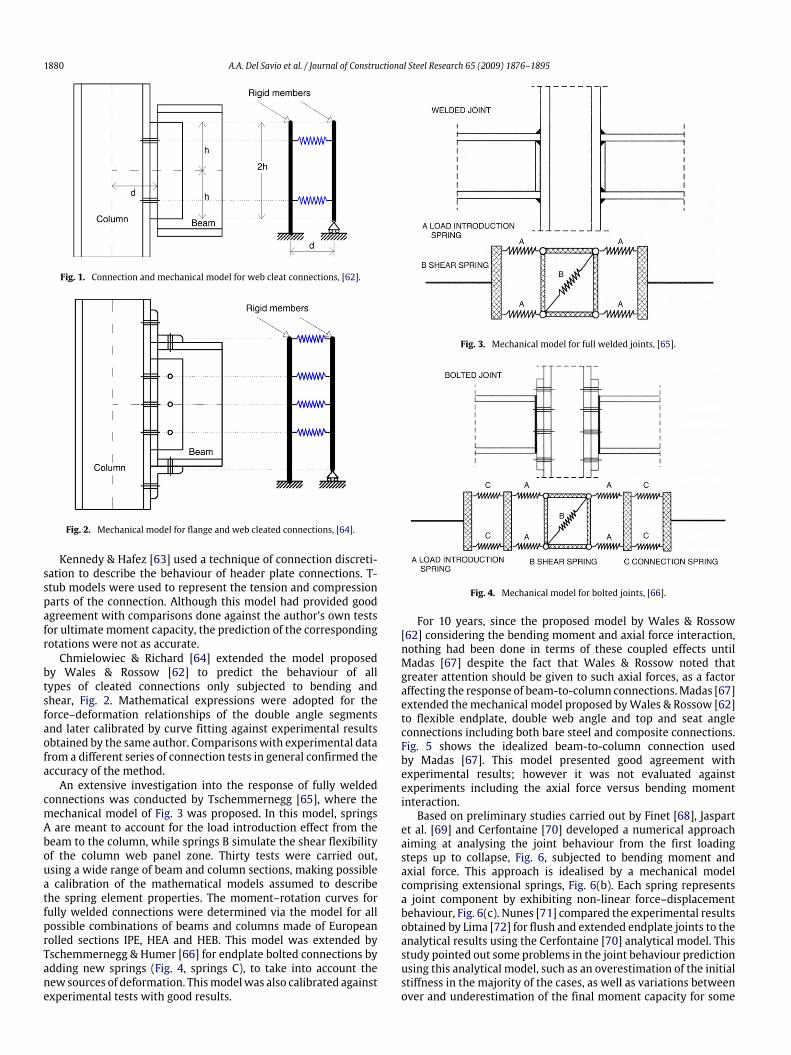
1880 A.A. Del Savio et al. / Journal of Constructional Steel Research 65 (2009) 1876–1895
Fig. 1. Connection and mechanical model for web cleat connections, [62].
Fig. 2. Mechanical model for flange and web cleated connections, [64].
Kennedy & Hafez [63] used a technique of connection discreti-sation to describe the behaviour of header plate connections. T-stub models were used to represent the tension and compressionparts of the connection. Although this model had provided goodagreement with comparisons done against the author’s own testsfor ultimate moment capacity, the prediction of the correspondingrotations were not as accurate.Chmielowiec & Richard [64] extended the model proposed
by Wales & Rossow [62] to predict the behaviour of alltypes of cleated connections only subjected to bending andshear, Fig. 2. Mathematical expressions were adopted for theforce–deformation relationships of the double angle segmentsand later calibrated by curve fitting against experimental resultsobtained by the same author. Comparisonswith experimental datafrom a different series of connection tests in general confirmed theaccuracy of the method.An extensive investigation into the response of fully welded
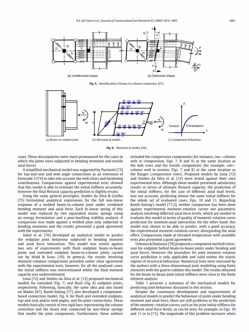
connections was conducted by Tschemmernegg [65], where themechanical model of Fig. 3 was proposed. In this model, springsA are meant to account for the load introduction effect from thebeam to the column, while springs B simulate the shear flexibilityof the column web panel zone. Thirty tests were carried out,using a wide range of beam and column sections, making possiblea calibration of the mathematical models assumed to describethe spring element properties. The moment–rotation curves forfully welded connections were determined via the model for allpossible combinations of beams and columns made of Europeanrolled sections IPE, HEA and HEB. This model was extended byTschemmernegg & Humer [66] for endplate bolted connections byadding new springs (Fig. 4, springs C), to take into account thenew sources of deformation. Thismodelwas also calibrated againstexperimental tests with good results.
Fig. 3. Mechanical model for full welded joints, [65].
Fig. 4. Mechanical model for bolted joints, [66].
For 10 years, since the proposed model by Wales & Rossow[62] considering the bending moment and axial force interaction,nothing had been done in terms of these coupled effects untilMadas [67] despite the fact that Wales & Rossow noted thatgreater attention should be given to such axial forces, as a factoraffecting the response of beam-to-column connections.Madas [67]extended themechanical model proposed byWales & Rossow [62]to flexible endplate, double web angle and top and seat angleconnections including both bare steel and composite connections.Fig. 5 shows the idealized beam-to-column connection usedby Madas [67]. This model presented good agreement withexperimental results; however it was not evaluated againstexperiments including the axial force versus bending momentinteraction.Based on preliminary studies carried out by Finet [68], Jaspart
et al. [69] and Cerfontaine [70] developed a numerical approachaiming at analysing the joint behaviour from the first loadingsteps up to collapse, Fig. 6, subjected to bending moment andaxial force. This approach is idealised by a mechanical modelcomprising extensional springs, Fig. 6(b). Each spring representsa joint component by exhibiting non-linear force–displacementbehaviour, Fig. 6(c). Nunes [71] compared the experimental resultsobtained by Lima [72] for flush and extended endplate joints to theanalytical results using the Cerfontaine [70] analytical model. Thisstudy pointed out some problems in the joint behaviour predictionusing this analytical model, such as an overestimation of the initialstiffness in the majority of the cases, as well as variations betweenover and underestimation of the final moment capacity for some
A.A. Del Savio et al. / Journal of Constructional Steel Research 65 (2009) 1876–1895 1881
Fig. 5. Identification of beam-to-column connection, [67].
(a) Beam-to-column joint. (b) Mechanical model. (c) Component behaviour.
Fig. 6. Mechanical model, [69].
cases. These discrepancies were more pronounced for the cases inwhich the joints were subjected to bending moments and tensileaxial forces.A simplified mechanical model was suggested by Pucinotti [73]
for top-and-seat and web angle connections as an extension ofEurocode 3 [74] to take into account the web cleats and hardeningcontributions. Comparisons against experimental tests showedthat this model is able to estimate the initial stiffness accurately;however the final flexural capacity prediction is slightly erratic.Using the same general principles, Simões da Silva & Coelho
[75] formulated analytical expressions for the full non-linearresponse of a welded beam-to-column joint under combinedbending moment and axial force. Each bi-linear spring of thismodel was replaced by two equivalent elastic springs usingan energy formulation and a post-buckling stability analysis. Acomparison was made against a welded joint only subjected tobending moments and the results presented a good agreementwith the experiments.Sokol et al. [76] developed an analytical model to predict
the endplate joint behaviour subjected to bending momentand axial force interaction. This model was tested againsttwo sets of experiments with flush endplate beam-to-beamjoints and extended endplate beam-to-column joints carriedout by Wald & Svarc [10]. In general, the results involvingmoment–rotation comparisons provided rather close agreementwith the experimental tests, however, for all the analysed cases,the initial stiffness was overestimated whilst the final momentcapacity was underestimated.Lima [72] and Simões da Silva et al. [12] proposed mechanical
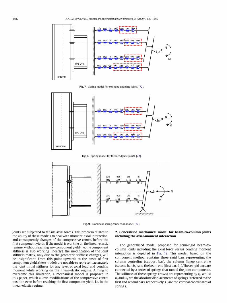
models for extended (Fig. 7) and flush (Fig. 8) endplate joints,respectively. Following, basically, the same idea and also basedon Madas [67], Ramli-Sulong [77] also developed a component-based connection model, Fig. 9, for flush and extended endplate,top-and-seat and/or web angles, and fin-plate connections. Thesemodels basically consist of two rigid bars representing the columncentreline and the beam end, connected by non-linear springsthat model the joint components. Furthermore, these authors
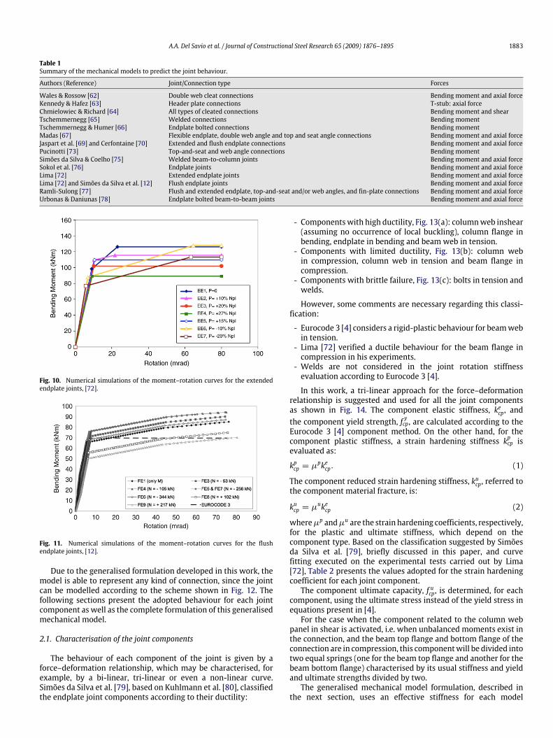
included the compressive components (for instance, cwc—columnweb in compression, Figs. 7, 8 and 9) at the same location asthe bolt rows and the tensile components (for example, cwt—column web in tension, Figs. 7 and 8) at the same location asthe flanges (compressive rows). Proposed models by Lima [72]and Simões da Silva et al. [12] were tested against their ownexperimental tests. Although these models presented satisfactoryresults in terms of ultimate flexural capacity, the prediction ofthe initial stiffness, for the case of different axial load levels,was not accurate, predicting almost the same initial stiffness forthe whole set of evaluated cases, Figs. 10 and 11. RegardingRamli-Sulong’s model [77,2], neither comparison has been doneagainst experimental moment–rotation curves nor parametricanalysis involving different axial force levels, which are needed toevaluate this model in terms of quality of moment–rotation curveprediction for moment-axial interaction. On the other hand, thismodel was shown to be able to predict, with a good accuracy,the experimental moment–rotation curves, disregarding the axialeffect. Comparisons made at elevated temperature with availabletests also presented a good agreement.Urbonas &Daniunas [78] proposed a componentmethod exten-
sion for endplate bolted beam-to-beam joints under bending andaxial forces. However the procedure for joint moment–rotationcurve prediction is only applicable and valid within the elasticregime of structural behaviour. Numerical tests were executed bythe authors with a three-dimensional joint modelling using finiteelements with the goal to validate this model. The results obtainedfor the beam-to-beam joint initial stiffness were close to the finiteelement analysis.Table 1 presents a summary of the mechanical models for
predicting joint behaviour discussed in this section.Despite the continuous development and improvement of
analytical models to predict the behaviour of joints under bendingmoment and axial force, there are still problems in the predictionof themoment–rotation curves, such as the joint initial stiffness fordifferent axial force levels, as can be seen, for example, in Figs. 10and 11 or in [71]. The magnitude of this problem increases when
1882 A.A. Del Savio et al. / Journal of Constructional Steel Research 65 (2009) 1876–1895
Fig. 7. Spring model for extended endplate joints, [72].
Fig. 8. Spring model for flush endplate joints, [72].
Fig. 9. Nonlinear spring connection model, [77].
joints are subjected to tensile axial forces. This problem relates tothe ability of these models to deal with moment-axial interaction,and consequently changes of the compressive centre, before thefirst component yields. If themodel isworking on the linear-elasticregime, without reaching any component yield (i.e. the componentstiffness is also working linearly), the modification of the jointstiffness matrix, only due to the geometric stiffness changes, willbe insignificant. From this point upwards to the onset of firstcomponent yield, thesemodels are not able to represent accuratelythe joint initial stiffness for any level of axial load and bendingmoment while working on the linear-elastic regime. Aiming toovercome this limitation, a mechanical model is proposed inthis paper, which allows modifications of the compressive centreposition even before reaching the first component yield, i.e. in thelinear-elastic regime.
2. Generalised mechanical model for beam-to-column jointsincluding the axial-moment interaction
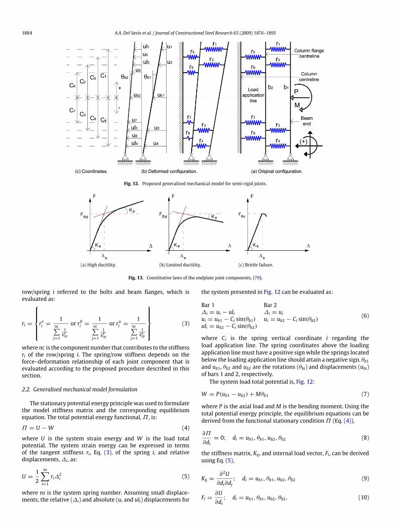
The generalised model proposed for semi-rigid beam-to-column joints including the axial force versus bending momentinteraction is depicted in Fig. 12. This model, based on thecomponent method, contains three rigid bars representing thecolumn centreline (support bar), the column flange centreline(second bar, b2) and the beamend (first bar, b1). These rigid bars areconnected by a series of springs that model the joint components.The stiffness of these springs (rows) are representing by ri, whilstui and uli are the absolute displacements of springs i referred to thefirst and second bars, respectively. Ci are the vertical coordinates ofspring i.
A.A. Del Savio et al. / Journal of Constructional Steel Research 65 (2009) 1876–1895 1883
Table 1Summary of the mechanical models to predict the joint behaviour.
Authors (Reference) Joint/Connection type Forces
Wales & Rossow [62] Double web cleat connections Bending moment and axial forceKennedy & Hafez [63] Header plate connections T-stub: axial forceChmielowiec & Richard [64] All types of cleated connections Bending moment and shearTschemmernegg [65] Welded connections Bending momentTschemmernegg & Humer [66] Endplate bolted connections Bending momentMadas [67] Flexible endplate, double web angle and top and seat angle connections Bending moment and axial forceJaspart et al. [69] and Cerfontaine [70] Extended and flush endplate connections Bending moment and axial forcePucinotti [73] Top-and-seat and web angle connections Bending momentSimões da Silva & Coelho [75] Welded beam-to-column joints Bending moment and axial forceSokol et al. [76] Endplate joints Bending moment and axial forceLima [72] Extended endplate joints Bending moment and axial forceLima [72] and Simões da Silva et al. [12] Flush endplate joints Bending moment and axial forceRamli-Sulong [77] Flush and extended endplate, top-and-seat and/or web angles, and fin-plate connections Bending moment and axial forceUrbonas & Daniunas [78] Endplate bolted beam-to-beam joints Bending moment and axial force
Fig. 10. Numerical simulations of the moment–rotation curves for the extendedendplate joints, [72].
Fig. 11. Numerical simulations of the moment–rotation curves for the flushendplate joints, [12].
Due to the generalised formulation developed in this work, themodel is able to represent any kind of connection, since the jointcan be modelled according to the scheme shown in Fig. 12. Thefollowing sections present the adopted behaviour for each jointcomponent as well as the complete formulation of this generalisedmechanical model.
2.1. Characterisation of the joint components
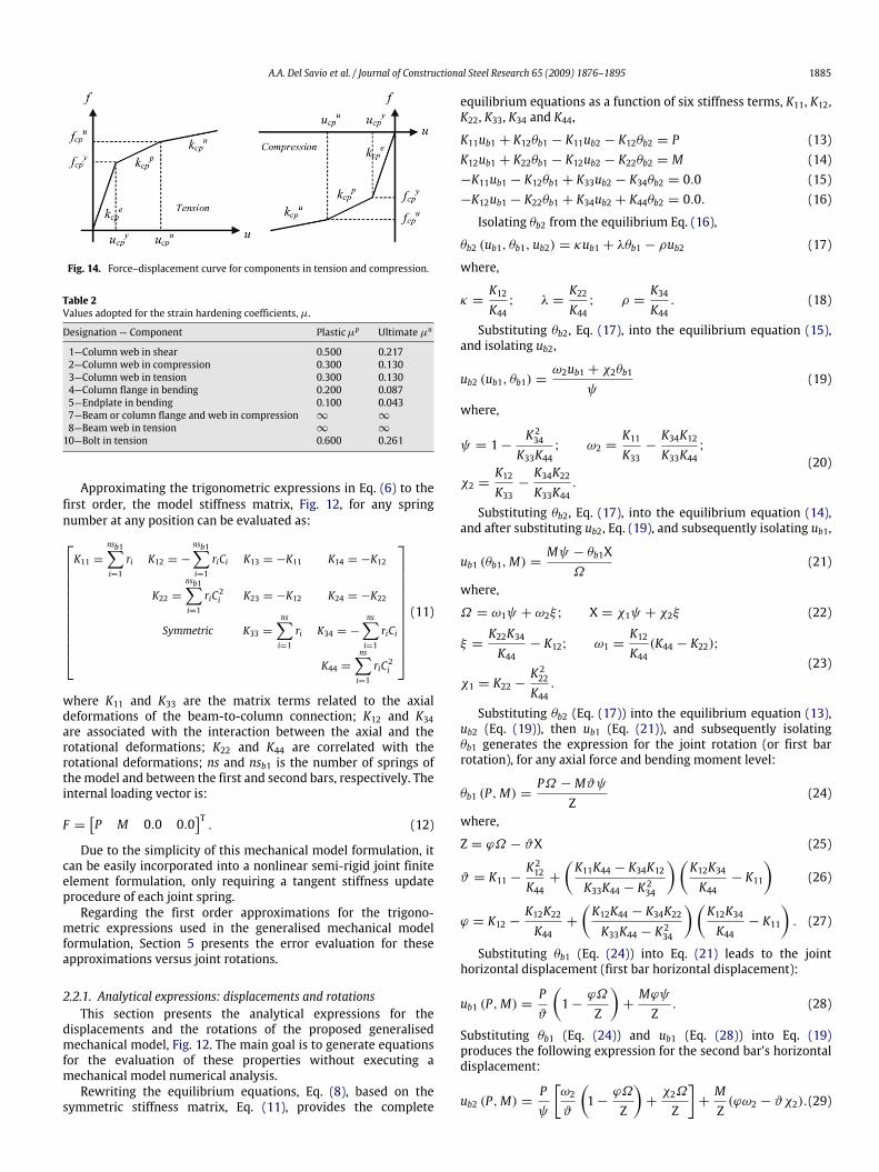
The behaviour of each component of the joint is given by aforce–deformation relationship, which may be characterised, forexample, by a bi-linear, tri-linear or even a non-linear curve.Simões da Silva et al. [79], based on Kuhlmann et al. [80], classifiedthe endplate joint components according to their ductility:
- Componentswith high ductility, Fig. 13(a): columnweb inshear(assuming no occurrence of local buckling), column flange inbending, endplate in bending and beam web in tension.- Components with limited ductility, Fig. 13(b): column webin compression, column web in tension and beam flange incompression.- Components with brittle failure, Fig. 13(c): bolts in tension andwelds.
However, some comments are necessary regarding this classi-fication:
- Eurocode 3 [4] considers a rigid-plastic behaviour for beamwebin tension.- Lima [72] verified a ductile behaviour for the beam flange incompression in his experiments.- Welds are not considered in the joint rotation stiffnessevaluation according to Eurocode 3 [4].
In this work, a tri-linear approach for the force–deformationrelationship is suggested and used for all the joint componentsas shown in Fig. 14. The component elastic stiffness, kecp, andthe component yield strength, f ycp, are calculated according to theEurocode 3 [4] component method. On the other hand, for thecomponent plastic stiffness, a strain hardening stiffness kpcp isevaluated as:
kpcp = µpkecp. (1)
The component reduced strain hardening stiffness, kucp, referred tothe component material fracture, is:
kucp = µukecp (2)
whereµp andµu are the strain hardening coefficients, respectively,for the plastic and ultimate stiffness, which depend on thecomponent type. Based on the classification suggested by Simõesda Silva et al. [79], briefly discussed in this paper, and curvefitting executed on the experimental tests carried out by Lima[72], Table 2 presents the values adopted for the strain hardeningcoefficient for each joint component.The component ultimate capacity, f ucp, is determined, for each
component, using the ultimate stress instead of the yield stress inequations present in [4].For the case when the component related to the column web
panel in shear is activated, i.e. when unbalanced moments exist inthe connection, and the beam top flange and bottom flange of theconnection are in compression, this componentwill be divided intotwo equal springs (one for the beam top flange and another for thebeam bottom flange) characterised by its usual stiffness and yieldand ultimate strengths divided by two.The generalised mechanical model formulation, described in
the next section, uses an effective stiffness for each model
1884 A.A. Del Savio et al. / Journal of Constructional Steel Research 65 (2009) 1876–1895
Fig. 12. Proposed generalised mechanical model for semi-rigid joints.
(a) High ductility. (b) Limited ductility. (c) Brittle failure.
Fig. 13. Constitutive laws of the endplate joint components, [79].
row/spring i referred to the bolts and beam flanges, which isevaluated as:
ri =
rei =
1nc∑j=1
1kecp
or rpi =1
nc∑j=1
1kpcp
or rui =1
nc∑j=1
1kucp
(3)
wherenc is the component number that contributes to the stiffnessri of the row/spring i. The spring/row stiffness depends on theforce–deformation relationship of each joint component that isevaluated according to the proposed procedure described in thissection.
2.2. Generalised mechanical model formulation
The stationary potential energy principlewas used to formulatethe model stiffness matrix and the corresponding equilibriumequation. The total potential energy functional,Π , is:
Π = U −W (4)
where U is the system strain energy and W is the load totalpotential. The system strain energy can be expressed in termsof the tangent stiffness ri, Eq. (3), of the spring i, and relativedisplacements,∆i, as:
U =12
ns∑i=1
ri∆2i (5)
where ns is the system spring number. Assuming small displace-ments, the relative (∆i) and absolute (ui and uli) displacements for
the system presented in Fig. 12 can be evaluated as:
Bar 1 Bar 2∆i = ui − uli ∆i = uiui = ub1 − Ci sin(θb1) ui = ub2 − Ci sin(θb2)uli = ub2 − Ci sin(θb2)
(6)
where Ci is the spring vertical coordinate i regarding theload application line. The spring coordinates above the loadingapplication linemust have a positive signwhile the springs locatedbelow the loading application line should attain a negative sign. θb1and ub1, θb2 and ub2 are the rotations (θbi) and displacements (ubi)of bars 1 and 2, respectively.The system load total potential is, Fig. 12:
W = P(ub1 − ub2)+Mθb1 (7)
where P is the axial load andM is the bending moment. Using thetotal potential energy principle, the equilibrium equations can bederived from the functional stationary conditionΠ (Eq. (4)),
∂Π
∂di= 0; di = ub1, θb1, ub2, θb2 (8)
the stiffness matrix, Kij, and internal load vector, Fi, can be derivedusing Eq. (5),
Kij =∂2U∂di∂dj
; di = ub1, θb1, ub2, θb2 (9)
Fi =∂U∂di; di = ub1, θb1, ub2, θb2. (10)
A.A. Del Savio et al. / Journal of Constructional Steel Research 65 (2009) 1876–1895 1885
Fig. 14. Force–displacement curve for components in tension and compression.
Table 2Values adopted for the strain hardening coefficients, µ.
Designation — Component Plasticµp Ultimate µu
1—Column web in shear 0.500 0.2172—Column web in compression 0.300 0.1303—Column web in tension 0.300 0.1304—Column flange in bending 0.200 0.0875—Endplate in bending 0.100 0.0437—Beam or column flange and web in compression ∞ ∞
8—Beam web in tension ∞ ∞
10—Bolt in tension 0.600 0.261
Approximating the trigonometric expressions in Eq. (6) to thefirst order, the model stiffness matrix, Fig. 12, for any springnumber at any position can be evaluated as:
K11 =nsb1∑i=1
ri K12 = −nsb1∑i=1
riCi K13 = −K11 K14 = −K12
K22 =nsb1∑i=1
riC2i K23 = −K12 K24 = −K22
Symmetric K33 =ns∑i=1
ri K34 = −ns∑i=1
riCi
K44 =ns∑i=1
riC2i
(11)
where K11 and K33 are the matrix terms related to the axialdeformations of the beam-to-column connection; K12 and K34are associated with the interaction between the axial and therotational deformations; K22 and K44 are correlated with therotational deformations; ns and nsb1 is the number of springs ofthe model and between the first and second bars, respectively. Theinternal loading vector is:
F =[P M 0.0 0.0
]T. (12)
Due to the simplicity of this mechanical model formulation, itcan be easily incorporated into a nonlinear semi-rigid joint finiteelement formulation, only requiring a tangent stiffness updateprocedure of each joint spring.Regarding the first order approximations for the trigono-
metric expressions used in the generalised mechanical modelformulation, Section 5 presents the error evaluation for theseapproximations versus joint rotations.
2.2.1. Analytical expressions: displacements and rotationsThis section presents the analytical expressions for the
displacements and the rotations of the proposed generalisedmechanical model, Fig. 12. The main goal is to generate equationsfor the evaluation of these properties without executing amechanical model numerical analysis.Rewriting the equilibrium equations, Eq. (8), based on the
symmetric stiffness matrix, Eq. (11), provides the complete
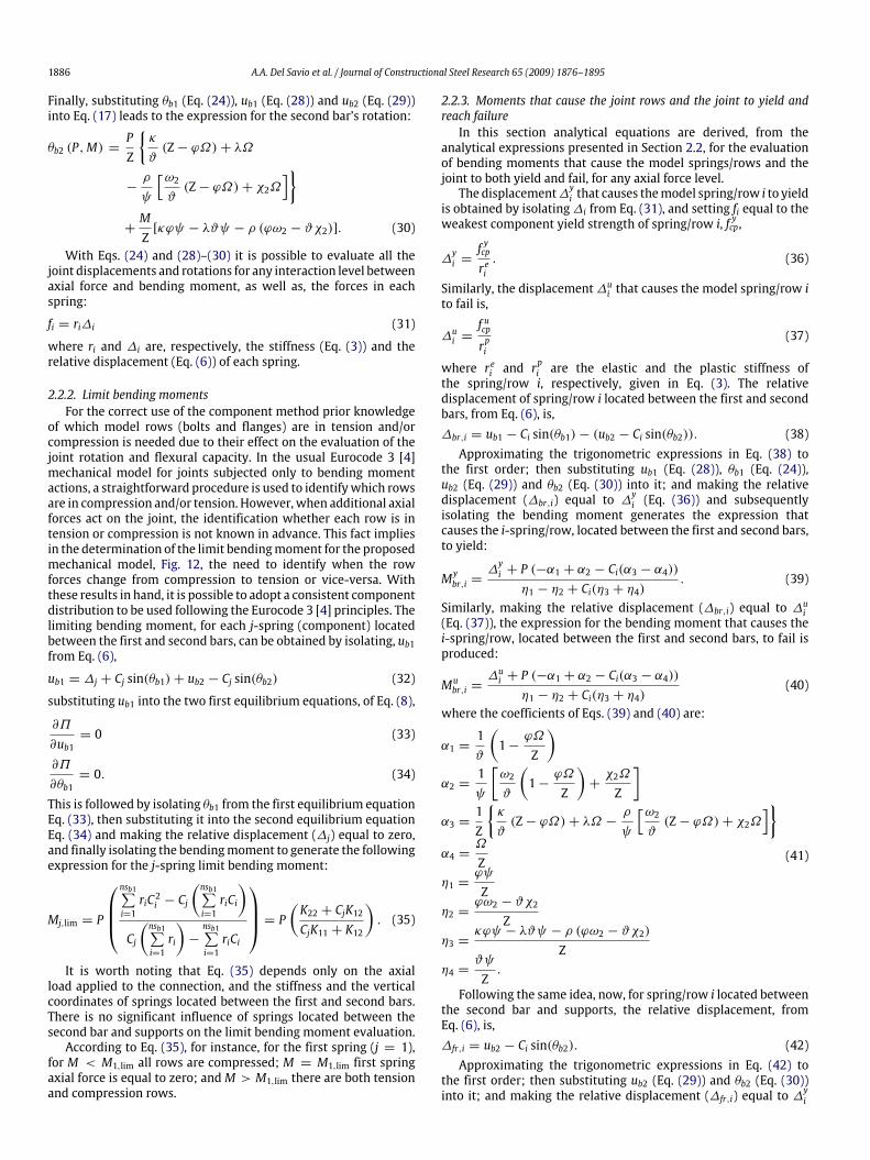
equilibrium equations as a function of six stiffness terms, K11, K12,K22, K33, K34 and K44,
K11ub1 + K12θb1 − K11ub2 − K12θb2 = P (13)K12ub1 + K22θb1 − K12ub2 − K22θb2 = M (14)−K11ub1 − K12θb1 + K33ub2 − K34θb2 = 0.0 (15)−K12ub1 − K22θb1 + K34ub2 + K44θb2 = 0.0. (16)
Isolating θb2 from the equilibrium Eq. (16),
θb2 (ub1, θb1, ub2) = κub1 + λθb1 − ρub2 (17)
where,
κ =K12K44; λ =
K22K44; ρ =
K34K44
. (18)
Substituting θb2, Eq. (17), into the equilibrium equation (15),and isolating ub2,
ub2 (ub1, θb1) =ω2ub1 + χ2θb1
ψ(19)
where,
ψ = 1−K 234K33K44
; ω2 =K11K33−K34K12K33K44
;
χ2 =K12K33−K34K22K33K44
.
(20)
Substituting θb2, Eq. (17), into the equilibrium equation (14),and after substituting ub2, Eq. (19), and subsequently isolating ub1,
ub1 (θb1,M) =Mψ − θb1X
Ω(21)
where,
Ω = ω1ψ + ω2ξ ; X = χ1ψ + χ2ξ (22)
ξ =K22K34K44
− K12; ω1 =K12K44
(K44 − K22);
χ1 = K22 −K 222K44
.
(23)
Substituting θb2 (Eq. (17)) into the equilibrium equation (13),ub2 (Eq. (19)), then ub1 (Eq. (21)), and subsequently isolatingθb1 generates the expression for the joint rotation (or first barrotation), for any axial force and bending moment level:
θb1 (P,M) =PΩ −Mϑψ
Z(24)
where,
Z = ϕΩ − ϑX (25)
ϑ = K11 −K 212K44+
(K11K44 − K34K12K33K44 − K 234
)(K12K34K44
− K11
)(26)
ϕ = K12 −K12K22K44
+
(K12K44 − K34K22K33K44 − K 234
)(K12K34K44
− K11
). (27)
Substituting θb1 (Eq. (24)) into Eq. (21) leads to the jointhorizontal displacement (first bar horizontal displacement):
ub1 (P,M) =Pϑ
(1−
ϕΩ
Z
)+MϕψZ
. (28)
Substituting θb1 (Eq. (24)) and ub1 (Eq. (28)) into Eq. (19)produces the following expression for the second bar’s horizontaldisplacement:
ub2 (P,M) =Pψ
[ω2
ϑ
(1−
ϕΩ
Z
)+χ2Ω
Z
]+MZ(ϕω2 − ϑχ2).(29)
1886 A.A. Del Savio et al. / Journal of Constructional Steel Research 65 (2009) 1876–1895
Finally, substituting θb1 (Eq. (24)), ub1 (Eq. (28)) and ub2 (Eq. (29))into Eq. (17) leads to the expression for the second bar’s rotation:
θb2 (P,M) =PZ
κ
ϑ(Z− ϕΩ)+ λΩ
−ρ
ψ
[ω2ϑ(Z− ϕΩ)+ χ2Ω
]+MZ[κϕψ − λϑψ − ρ (ϕω2 − ϑχ2)]. (30)
With Eqs. (24) and (28)–(30) it is possible to evaluate all thejoint displacements and rotations for any interaction level betweenaxial force and bending moment, as well as, the forces in eachspring:
fi = ri∆i (31)
where ri and ∆i are, respectively, the stiffness (Eq. (3)) and therelative displacement (Eq. (6)) of each spring.
2.2.2. Limit bending momentsFor the correct use of the component method prior knowledge
of which model rows (bolts and flanges) are in tension and/orcompression is needed due to their effect on the evaluation of thejoint rotation and flexural capacity. In the usual Eurocode 3 [4]mechanical model for joints subjected only to bending momentactions, a straightforward procedure is used to identifywhich rowsare in compression and/or tension. However, when additional axialforces act on the joint, the identification whether each row is intension or compression is not known in advance. This fact impliesin the determination of the limit bendingmoment for the proposedmechanical model, Fig. 12, the need to identify when the rowforces change from compression to tension or vice-versa. Withthese results in hand, it is possible to adopt a consistent componentdistribution to be used following the Eurocode 3 [4] principles. Thelimiting bending moment, for each j-spring (component) locatedbetween the first and second bars, can be obtained by isolating, ub1from Eq. (6),
ub1 = ∆j + Cj sin(θb1)+ ub2 − Cj sin(θb2) (32)
substituting ub1 into the two first equilibrium equations, of Eq. (8),
∂Π
∂ub1= 0 (33)
∂Π
∂θb1= 0. (34)
This is followed by isolating θb1 from the first equilibrium equationEq. (33), then substituting it into the second equilibrium equationEq. (34) and making the relative displacement (∆j) equal to zero,and finally isolating the bendingmoment to generate the followingexpression for the j-spring limit bending moment:
Mj,lim = P
nsb1∑i=1riC2i − Cj
(nsb1∑i=1riCi
)Cj
(nsb1∑i=1ri
)−
nsb1∑i=1riCi
= P (K22 + CjK12CjK11 + K12
). (35)
It is worth noting that Eq. (35) depends only on the axialload applied to the connection, and the stiffness and the verticalcoordinates of springs located between the first and second bars.There is no significant influence of springs located between thesecond bar and supports on the limit bending moment evaluation.According to Eq. (35), for instance, for the first spring (j = 1),
for M < M1,lim all rows are compressed; M = M1,lim first springaxial force is equal to zero; andM > M1,lim there are both tensionand compression rows.
2.2.3. Moments that cause the joint rows and the joint to yield andreach failureIn this section analytical equations are derived, from the
analytical expressions presented in Section 2.2, for the evaluationof bending moments that cause the model springs/rows and thejoint to both yield and fail, for any axial force level.The displacement∆yi that causes themodel spring/row i to yield
is obtained by isolating∆i from Eq. (31), and setting fi equal to theweakest component yield strength of spring/row i, f ycp,
∆yi =
f ycprei. (36)
Similarly, the displacement∆ui that causes the model spring/row ito fail is,
∆ui =f ucprpi
(37)
where rei and rpi are the elastic and the plastic stiffness of
the spring/row i, respectively, given in Eq. (3). The relativedisplacement of spring/row i located between the first and secondbars, from Eq. (6), is,∆br,i = ub1 − Ci sin(θb1)− (ub2 − Ci sin(θb2)). (38)Approximating the trigonometric expressions in Eq. (38) to
the first order; then substituting ub1 (Eq. (28)), θb1 (Eq. (24)),ub2 (Eq. (29)) and θb2 (Eq. (30)) into it; and making the relativedisplacement (∆br,i) equal to ∆
yi (Eq. (36)) and subsequently
isolating the bending moment generates the expression thatcauses the i-spring/row, located between the first and second bars,to yield:
Mybr,i =∆yi + P (−α1 + α2 − Ci(α3 − α4))
η1 − η2 + Ci(η3 + η4). (39)
Similarly, making the relative displacement (∆br,i) equal to ∆ui(Eq. (37)), the expression for the bending moment that causes thei-spring/row, located between the first and second bars, to fail isproduced:
Mubr,i =∆ui + P (−α1 + α2 − Ci(α3 − α4))
η1 − η2 + Ci(η3 + η4)(40)
where the coefficients of Eqs. (39) and (40) are:
α1 =1ϑ
(1−
ϕΩ
Z
)α2 =
1ψ
[ω2
ϑ
(1−
ϕΩ
Z
)+χ2Ω
Z
]α3 =
1Z
κ
ϑ(Z− ϕΩ)+ λΩ −
ρ
ψ
[ω2ϑ(Z− ϕΩ)+ χ2Ω
]α4 =
Ω
Zη1 =
ϕψ
Zη2 =
ϕω2 − ϑχ2
Zη3 =
κϕψ − λϑψ − ρ (ϕω2 − ϑχ2)
Zη4 =
ϑψ
Z.
(41)
Following the same idea, now, for spring/row i located betweenthe second bar and supports, the relative displacement, fromEq. (6), is,∆fr,i = ub2 − Ci sin(θb2). (42)Approximating the trigonometric expressions in Eq. (42) to
the first order; then substituting ub2 (Eq. (29)) and θb2 (Eq. (30))into it; and making the relative displacement (∆fr,i) equal to ∆
yi
A.A. Del Savio et al. / Journal of Constructional Steel Research 65 (2009) 1876–1895 1887
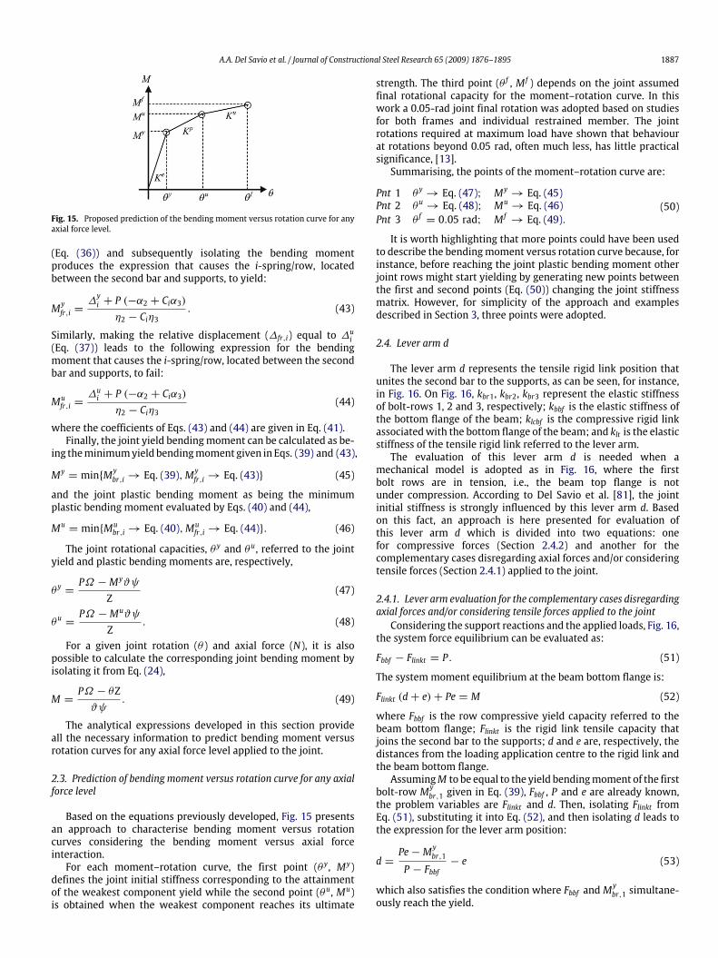
Fig. 15. Proposed prediction of the bending moment versus rotation curve for anyaxial force level.
(Eq. (36)) and subsequently isolating the bending momentproduces the expression that causes the i-spring/row, locatedbetween the second bar and supports, to yield:
Myfr,i =∆yi + P (−α2 + Ciα3)
η2 − Ciη3. (43)
Similarly, making the relative displacement (∆fr,i) equal to ∆ui(Eq. (37)) leads to the following expression for the bendingmoment that causes the i-spring/row, located between the secondbar and supports, to fail:
Mufr,i =∆ui + P (−α2 + Ciα3)
η2 − Ciη3(44)
where the coefficients of Eqs. (43) and (44) are given in Eq. (41).Finally, the joint yield bendingmoment can be calculated as be-
ing theminimumyield bendingmoment given in Eqs. (39) and (43),
My = minMybr,i → Eq. (39),Myfr,i → Eq. (43) (45)
and the joint plastic bending moment as being the minimumplastic bending moment evaluated by Eqs. (40) and (44),
Mu = minMubr,i → Eq. (40),Mufr,i → Eq. (44). (46)
The joint rotational capacities, θ y and θu, referred to the jointyield and plastic bending moments are, respectively,
θ y =PΩ −Myϑψ
Z(47)
θu =PΩ −Muϑψ
Z. (48)
For a given joint rotation (θ ) and axial force (N), it is alsopossible to calculate the corresponding joint bending moment byisolating it from Eq. (24),
M =PΩ − θZϑψ
. (49)
The analytical expressions developed in this section provideall the necessary information to predict bending moment versusrotation curves for any axial force level applied to the joint.
2.3. Prediction of bending moment versus rotation curve for any axialforce level
Based on the equations previously developed, Fig. 15 presentsan approach to characterise bending moment versus rotationcurves considering the bending moment versus axial forceinteraction.For each moment–rotation curve, the first point (θ y, My)
defines the joint initial stiffness corresponding to the attainmentof the weakest component yield while the second point (θu, Mu)is obtained when the weakest component reaches its ultimate
strength. The third point (θ f , M f ) depends on the joint assumedfinal rotational capacity for the moment–rotation curve. In thiswork a 0.05-rad joint final rotation was adopted based on studiesfor both frames and individual restrained member. The jointrotations required at maximum load have shown that behaviourat rotations beyond 0.05 rad, often much less, has little practicalsignificance, [13].Summarising, the points of the moment–rotation curve are:
Pnt 1 θ y → Eq. (47); My → Eq. (45)Pnt 2 θu → Eq. (48); Mu → Eq. (46)Pnt 3 θ f = 0.05 rad; M f → Eq. (49).
(50)
It is worth highlighting that more points could have been usedto describe the bendingmoment versus rotation curve because, forinstance, before reaching the joint plastic bending moment otherjoint rows might start yielding by generating new points betweenthe first and second points (Eq. (50)) changing the joint stiffnessmatrix. However, for simplicity of the approach and examplesdescribed in Section 3, three points were adopted.
2.4. Lever arm d
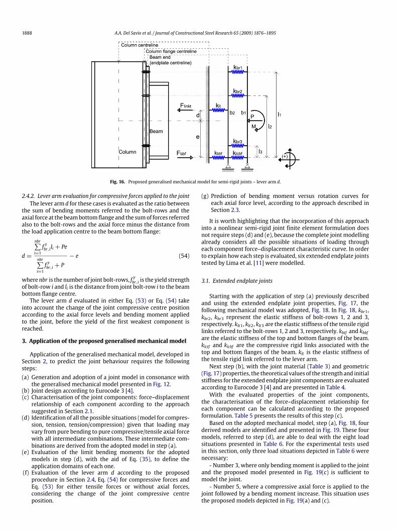
The lever arm d represents the tensile rigid link position thatunites the second bar to the supports, as can be seen, for instance,in Fig. 16. On Fig. 16, kbr1, kbr2, kbr3 represent the elastic stiffnessof bolt-rows 1, 2 and 3, respectively; kbbf is the elastic stiffness ofthe bottom flange of the beam; klcbf is the compressive rigid linkassociatedwith the bottom flange of the beam; and klt is the elasticstiffness of the tensile rigid link referred to the lever arm.The evaluation of this lever arm d is needed when a
mechanical model is adopted as in Fig. 16, where the firstbolt rows are in tension, i.e., the beam top flange is notunder compression. According to Del Savio et al. [81], the jointinitial stiffness is strongly influenced by this lever arm d. Basedon this fact, an approach is here presented for evaluation ofthis lever arm d which is divided into two equations: onefor compressive forces (Section 2.4.2) and another for thecomplementary cases disregarding axial forces and/or consideringtensile forces (Section 2.4.1) applied to the joint.
2.4.1. Lever arm evaluation for the complementary cases disregardingaxial forces and/or considering tensile forces applied to the jointConsidering the support reactions and the applied loads, Fig. 16,
the system force equilibrium can be evaluated as:
Fbbf − Flinkt = P. (51)
The system moment equilibrium at the beam bottom flange is:
Flinkt (d+ e)+ Pe = M (52)
where Fbbf is the row compressive yield capacity referred to thebeam bottom flange; Flinkt is the rigid link tensile capacity thatjoins the second bar to the supports; d and e are, respectively, thedistances from the loading application centre to the rigid link andthe beam bottom flange.AssumingM to be equal to the yield bendingmoment of the first
bolt-row Mybr,1 given in Eq. (39), Fbbf , P and e are already known,the problem variables are Flinkt and d. Then, isolating Flinkt fromEq. (51), substituting it into Eq. (52), and then isolating d leads tothe expression for the lever arm position:
d =Pe−Mybr,1P − Fbbf
− e (53)
which also satisfies the condition where Fbbf andMybr,1 simultane-
ously reach the yield.
1888 A.A. Del Savio et al. / Journal of Constructional Steel Research 65 (2009) 1876–1895
Fig. 16. Proposed generalised mechanical model for semi-rigid joints – lever arm d.
2.4.2. Lever arm evaluation for compressive forces applied to the jointThe lever arm d for these cases is evaluated as the ratio between
the sum of bending moments referred to the bolt-rows and theaxial force at the beambottom flange and the sumof forces referredalso to the bolt-rows and the axial force minus the distance fromthe load application centre to the beam bottom flange:
d =
nbr∑i=1f ybr,ili + Pe
nbr∑i=1f ybr,i + P
− e (54)
where nbr is the number of joint bolt-rows, f ybr,i is the yield strengthof bolt-row i and li is the distance from joint bolt-row i to the beambottom flange centre.The lever arm d evaluated in either Eq. (53) or Eq. (54) take
into account the change of the joint compressive centre positionaccording to the axial force levels and bending moment appliedto the joint, before the yield of the first weakest component isreached.
3. Application of the proposed generalised mechanical model
Application of the generalised mechanical model, developed inSection 2, to predict the joint behaviour requires the followingsteps:(a) Generation and adoption of a joint model in consonance withthe generalised mechanical model presented in Fig. 12.
(b) Joint design according to Eurocode 3 [4].(c) Characterisation of the joint components: force–displacementrelationship of each component according to the approachsuggested in Section 2.1.
(d) Identification of all the possible situations (model for compres-sion, tension, tension/compression) given that loading mayvary from pure bending to pure compressive/tensile axial forcewith all intermediate combinations. These intermediate com-binations are derived from the adopted model in step (a).
(e) Evaluation of the limit bending moments for the adoptedmodels in step (d), with the aid of Eq. (35), to define theapplication domains of each one.
(f) Evaluation of the lever arm d according to the proposedprocedure in Section 2.4, Eq. (54) for compressive forces andEq. (53) for either tensile forces or without axial forces,considering the change of the joint compressive centreposition.
(g) Prediction of bending moment versus rotation curves foreach axial force level, according to the approach described inSection 2.3.
It is worth highlighting that the incorporation of this approachinto a nonlinear semi-rigid joint finite element formulation doesnot require steps (d) and (e), because the complete joint modellingalready considers all the possible situations of loading througheach component force–displacement characteristic curve. In orderto explain how each step is evaluated, six extended endplate jointstested by Lima et al. [11] were modelled.
3.1. Extended endplate joints
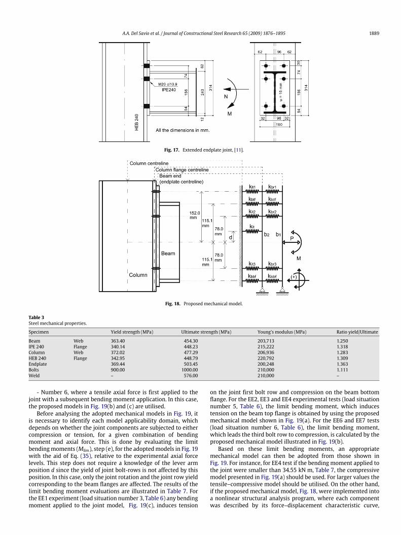
Starting with the application of step (a) previously describedand using the extended endplate joint properties, Fig. 17, thefollowing mechanical model was adopted, Fig. 18. In Fig. 18, kbr1,kbr2, kbr3 represent the elastic stiffness of bolt-rows 1, 2 and 3,respectively. klt1, klt2, klt3 are the elastic stiffness of the tensile rigidlinks referred to the bolt-rows 1, 2 and 3, respectively. kbtf and kbbfare the elastic stiffness of the top and bottom flanges of the beam.klctf and klcbf are the compressive rigid links associated with thetop and bottom flanges of the beam. klt is the elastic stiffness ofthe tensile rigid link referred to the lever arm.Next step (b), with the joint material (Table 3) and geometric
(Fig. 17) properties, the theoretical values of the strength and initialstiffness for the extended endplate joint components are evaluatedaccording to Eurocode 3 [4] and are presented in Table 4.With the evaluated properties of the joint components,
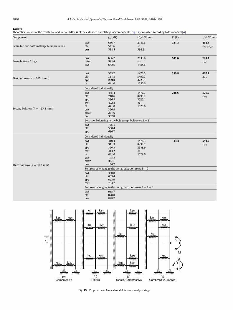
the characterisation of the force–displacement relationship foreach component can be calculated according to the proposedformulation. Table 5 presents the results of this step (c).Based on the adopted mechanical model, step (a), Fig. 18, four
derived models are identified and presented in Fig. 19. These fourmodels, referred to step (d), are able to deal with the eight loadsituations presented in Table 6. For the experimental tests usedin this section, only three load situations depicted in Table 6 werenecessary:- Number 3, where only bending moment is applied to the joint
and the proposed model presented in Fig. 19(c) is sufficient tomodel the joint.- Number 5, where a compressive axial force is applied to the
joint followed by a bending moment increase. This situation usesthe proposed models depicted in Fig. 19(a) and (c).
A.A. Del Savio et al. / Journal of Constructional Steel Research 65 (2009) 1876–1895 1889
Fig. 17. Extended endplate joint, [11].
Fig. 18. Proposed mechanical model.
Table 3Steel mechanical properties.
Specimen Yield strength (MPa) Ultimate strength (MPa) Young’s modulus (MPa) Ratio yield/Ultimate
Beam Web 363.40 454.30 203,713 1.250IPE 240 Flange 340.14 448.23 215,222 1.318Column Web 372.02 477.29 206,936 1.283HEB 240 Flange 342.95 448.79 220,792 1.309Endplate 369.44 503.45 200,248 1.363Bolts 900.00 1000.00 210,000 1.111Weld – 576.00 210,000 –
- Number 6, where a tensile axial force is first applied to thejoint with a subsequent bending moment application. In this case,the proposed models in Fig. 19(b) and (c) are utilised.Before analysing the adopted mechanical models in Fig. 19, it
is necessary to identify each model applicability domain, whichdepends on whether the joint components are subjected to eithercompression or tension, for a given combination of bendingmoment and axial force. This is done by evaluating the limitbendingmoments (Mlim), step (e), for the adoptedmodels in Fig. 19with the aid of Eq. (35), relative to the experimental axial forcelevels. This step does not require a knowledge of the lever armposition d since the yield of joint bolt-rows is not affected by thisposition. In this case, only the joint rotation and the joint row yieldcorresponding to the beam flanges are affected. The results of thelimit bending moment evaluations are illustrated in Table 7. Forthe EE1 experiment (load situation number 3, Table 6) any bendingmoment applied to the joint model, Fig. 19(c), induces tension
on the joint first bolt row and compression on the beam bottomflange. For the EE2, EE3 and EE4 experimental tests (load situationnumber 5, Table 6), the limit bending moment, which inducestension on the beam top flange is obtained by using the proposedmechanical model shown in Fig. 19(a). For the EE6 and EE7 tests(load situation number 6, Table 6), the limit bending moment,which leads the third bolt row to compression, is calculated by theproposed mechanical model illustrated in Fig. 19(b).Based on these limit bending moments, an appropriate
mechanical model can then be adopted from those shown inFig. 19. For instance, for EE4 test if the bending moment applied tothe joint were smaller than 34.55 kN m, Table 7, the compressivemodel presented in Fig. 19(a) should be used. For larger values thetensile–compressive model should be utilised. On the other hand,if the proposed mechanical model, Fig. 18, were implemented intoa nonlinear structural analysis program, where each componentwas described by its force–displacement characteristic curve,
1890 A.A. Del Savio et al. / Journal of Constructional Steel Research 65 (2009) 1876–1895
Table 4Theoretical values of the resistance and initial stiffness of the extended endplate joint components, Fig. 17, evaluated according to Eurocode 3 [4].
Component f ycp (kN) kecp (kN/mm) f yi (kN) rei (kN/mm)
Beam top and bottom flange (compression)cwc 656.7 2133.6 321.3 464.8bfc 541.6 ∞ kbtb /kbbfcws 321.3 594.3
Beam bottom flangecwc 656.7 2133.6 541.6 763.4bfwc 541.6 ∞ kbbfcws 642.5 1188.6
First bolt row (h = 267.1 mm)
cwt 533.2 1476.3 289.8 607.7cfb 311.3 8499.7 kbr1epb 289.8 4223.1bt 441.0 1630.6
Second bolt row (h = 193.1 mm)
Considered individuallycwt 445.4 1476.3 218.6 575.0cfb 218.6 8498.7 kbr2epb 326.9 3026.1bwt 492.3 ∞
bt 441.0 1629.6cwc 366.9bfwc 251.6cws 352.8Bolt-row belonging to the bolt group: bolt-rows 2+ 1cwt 735.1cfb 508.4epb 616.7
Third bolt row (h = 37.1 mm)
Considered individuallycwt 410.3 1476.3 33.3 554.7cfb 311.3 8498.7 kbr3epb 320.3 2538.9bwt 413.2 ∞
bt 441.0 1629.6cwc 148.3bfwc 33.3cws 134.2Bolt row belonging to the bolt group: bolt rows 3+ 2cwt 350.8cfb 663.4epb 623.9bwt 764.7Bolt row belonging to the bolt group: bolt rows 3+ 2+ 1cwt 918.7cfb 878.8cws 898.2
Fig. 19. Proposed mechanical model for each analysis stage.
A.A. Del Savio et al. / Journal of Constructional Steel Research 65 (2009) 1876–1895 1891
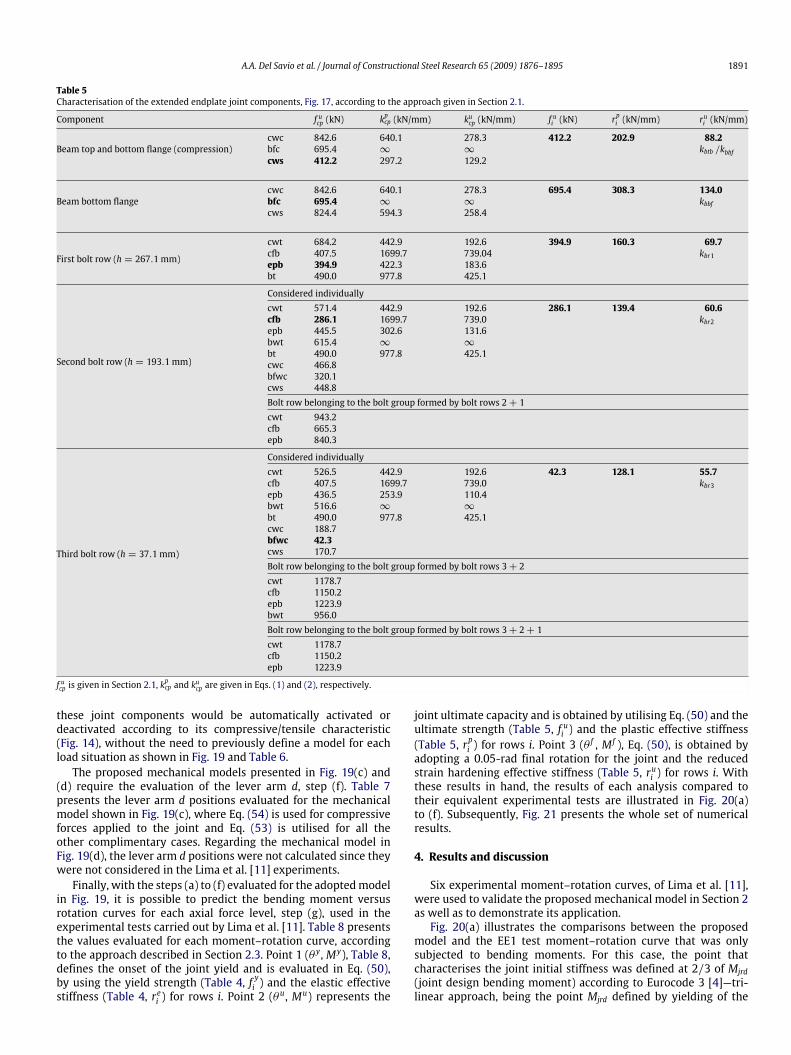
Table 5Characterisation of the extended endplate joint components, Fig. 17, according to the approach given in Section 2.1.
Component f ucp (kN) kpcp (kN/mm) kucp (kN/mm) f ui (kN) rpi (kN/mm) rui (kN/mm)
Beam top and bottom flange (compression)cwc 842.6 640.1 278.3 412.2 202.9 88.2bfc 695.4 ∞ ∞ kbtb /kbbfcws 412.2 297.2 129.2
Beam bottom flangecwc 842.6 640.1 278.3 695.4 308.3 134.0bfc 695.4 ∞ ∞ kbbfcws 824.4 594.3 258.4
First bolt row (h = 267.1 mm)
cwt 684.2 442.9 192.6 394.9 160.3 69.7cfb 407.5 1699.7 739.04 kbr1epb 394.9 422.3 183.6bt 490.0 977.8 425.1
Second bolt row (h = 193.1 mm)
Considered individuallycwt 571.4 442.9 192.6 286.1 139.4 60.6cfb 286.1 1699.7 739.0 kbr2epb 445.5 302.6 131.6bwt 615.4 ∞ ∞
bt 490.0 977.8 425.1cwc 466.8bfwc 320.1cws 448.8Bolt row belonging to the bolt group formed by bolt rows 2+ 1cwt 943.2cfb 665.3epb 840.3
Third bolt row (h = 37.1 mm)
Considered individuallycwt 526.5 442.9 192.6 42.3 128.1 55.7cfb 407.5 1699.7 739.0 kbr3epb 436.5 253.9 110.4bwt 516.6 ∞ ∞
bt 490.0 977.8 425.1cwc 188.7bfwc 42.3cws 170.7Bolt row belonging to the bolt group formed by bolt rows 3+ 2cwt 1178.7cfb 1150.2epb 1223.9bwt 956.0Bolt row belonging to the bolt group formed by bolt rows 3+ 2+ 1cwt 1178.7cfb 1150.2epb 1223.9
f ucp is given in Section 2.1, kpcp and kucp are given in Eqs. (1) and (2), respectively.
these joint components would be automatically activated ordeactivated according to its compressive/tensile characteristic(Fig. 14), without the need to previously define a model for eachload situation as shown in Fig. 19 and Table 6.The proposed mechanical models presented in Fig. 19(c) and
(d) require the evaluation of the lever arm d, step (f). Table 7presents the lever arm d positions evaluated for the mechanicalmodel shown in Fig. 19(c), where Eq. (54) is used for compressiveforces applied to the joint and Eq. (53) is utilised for all theother complimentary cases. Regarding the mechanical model inFig. 19(d), the lever arm d positions were not calculated since theywere not considered in the Lima et al. [11] experiments.Finally, with the steps (a) to (f) evaluated for the adoptedmodel
in Fig. 19, it is possible to predict the bending moment versusrotation curves for each axial force level, step (g), used in theexperimental tests carried out by Lima et al. [11]. Table 8 presentsthe values evaluated for each moment–rotation curve, accordingto the approach described in Section 2.3. Point 1 (θ y, My), Table 8,defines the onset of the joint yield and is evaluated in Eq. (50),by using the yield strength (Table 4, f yi ) and the elastic effectivestiffness (Table 4, rei ) for rows i. Point 2 (θ
u, Mu) represents the
joint ultimate capacity and is obtained by utilising Eq. (50) and theultimate strength (Table 5, f ui ) and the plastic effective stiffness(Table 5, rpi ) for rows i. Point 3 (θ
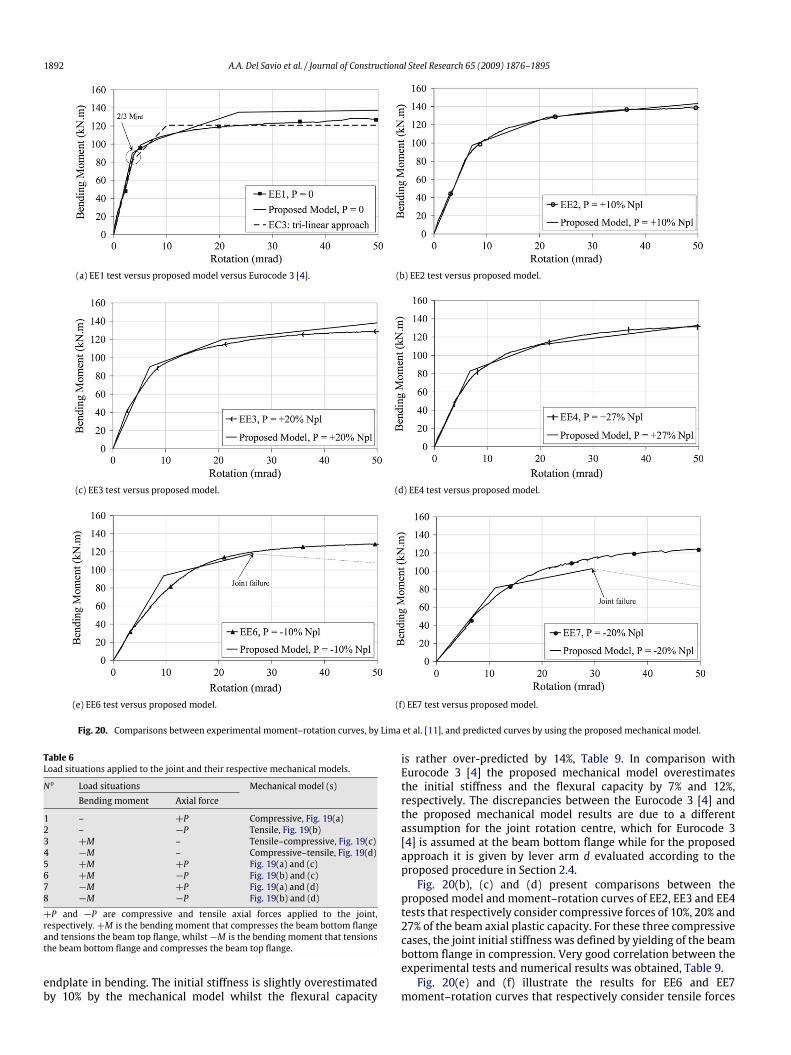
f , M f ), Eq. (50), is obtained byadopting a 0.05-rad final rotation for the joint and the reducedstrain hardening effective stiffness (Table 5, rui ) for rows i. Withthese results in hand, the results of each analysis compared totheir equivalent experimental tests are illustrated in Fig. 20(a)to (f). Subsequently, Fig. 21 presents the whole set of numericalresults.
4. Results and discussion
Six experimental moment–rotation curves, of Lima et al. [11],were used to validate the proposed mechanical model in Section 2as well as to demonstrate its application.Fig. 20(a) illustrates the comparisons between the proposed
model and the EE1 test moment–rotation curve that was onlysubjected to bending moments. For this case, the point thatcharacterises the joint initial stiffness was defined at 2/3 of Mjrd(joint design bending moment) according to Eurocode 3 [4]—tri-linear approach, being the point Mjrd defined by yielding of the
1892 A.A. Del Savio et al. / Journal of Constructional Steel Research 65 (2009) 1876–1895
(a) EE1 test versus proposed model versus Eurocode 3 [4]. (b) EE2 test versus proposed model.
(c) EE3 test versus proposed model. (d) EE4 test versus proposed model.
(e) EE6 test versus proposed model. (f) EE7 test versus proposed model.
Fig. 20. Comparisons between experimental moment–rotation curves, by Lima et al. [11], and predicted curves by using the proposed mechanical model.
Table 6Load situations applied to the joint and their respective mechanical models.
No Load situations Mechanical model (s)Bending moment Axial force
1 – +P Compressive, Fig. 19(a)2 – −P Tensile, Fig. 19(b)3 +M – Tensile–compressive, Fig. 19(c)4 −M – Compressive–tensile, Fig. 19(d)5 +M +P Fig. 19(a) and (c)6 +M −P Fig. 19(b) and (c)7 −M +P Fig. 19(a) and (d)8 −M −P Fig. 19(b) and (d)
+P and −P are compressive and tensile axial forces applied to the joint,respectively.+M is the bending moment that compresses the beam bottom flangeand tensions the beam top flange, whilst−M is the bending moment that tensionsthe beam bottom flange and compresses the beam top flange.
endplate in bending. The initial stiffness is slightly overestimatedby 10% by the mechanical model whilst the flexural capacity
is rather over-predicted by 14%, Table 9. In comparison withEurocode 3 [4] the proposed mechanical model overestimatesthe initial stiffness and the flexural capacity by 7% and 12%,respectively. The discrepancies between the Eurocode 3 [4] andthe proposed mechanical model results are due to a differentassumption for the joint rotation centre, which for Eurocode 3[4] is assumed at the beam bottom flange while for the proposedapproach it is given by lever arm d evaluated according to theproposed procedure in Section 2.4.Fig. 20(b), (c) and (d) present comparisons between the
proposed model and moment–rotation curves of EE2, EE3 and EE4tests that respectively consider compressive forces of 10%, 20% and27% of the beam axial plastic capacity. For these three compressivecases, the joint initial stiffness was defined by yielding of the beambottom flange in compression. Very good correlation between theexperimental tests and numerical results was obtained, Table 9.Fig. 20(e) and (f) illustrate the results for EE6 and EE7
moment–rotation curves that respectively consider tensile forces
A.A. Del Savio et al. / Journal of Constructional Steel Research 65 (2009) 1876–1895 1893
Table 7Applicability of each model,Mlim , and evaluation of lever arm d according to the experimental axial force levels.
Experimental data Mlim (kN m), Eq. (35) Lever arm (mm)Test N (kN) Compressive Fig. 19(a) Tensile Fig. 19(b) Tensile-compressive Fig. 19(c)
EE1 (only M) 0.00 NAa NAa 0.00 toM f Eq. (53): 79.28EE2 (+10% Npl) 135.94 0.0 to 18.12 NAa 18.12 toM f Eq. (54): 86.34EE3 (+20% Npl) 193.30 0.0 to 25.77 NAa 25.77 toM f Eq. (54): 79.60EE4 (+27% Npl) 259.20 0.0 to 34.55 NAa 34.55 toM f Eq. (54): 73.05EE6 (−10% Npl) −127.20 NAa 0.0 to 15.96 13.73 toM f Eq. (53): 46.57EE7 (−20% Npl) −257.90 NAa 0.0 to 32.36 27.84 toM f Eq. (53): 24.33
‘‘+’’ indicates compressive axial forces and ‘‘−’’ tensile axial forces.M f is given in Eq. (50).a NA= not applicable.
Table 8Values evaluated for the prediction of the moment–rotation curves for different axial force levels.
Point EE1 (onlyM) EE2 (+10%Npl) EE3 (+20%Npl) EE4 (+27%Npl) EE6 (−10%Npl) EE7 (−20%Npl)θ M θ M θ M θ M θ M θ M(mrad) (kN m) (mrad) (kN m) (mrad) (kN m) (mrad) (kN m) (mrad) (kN m) (mrad) (kN m)
0.0 0.0 0.0 0.0 0.0 0.0 0.0 0.0 0.0 0.0 0.0 0.01 8.2 105.3 7.2 97.4 7.0 90.1 6.7 83.0 9.6 93.5 11.1 81.42 23.6 135.1 21.4 128.2 20.8 119.9 20.1 111.8 26.4 118.3 29.5 102.73 50.0 137.3 50.0 143.3 50.0 138.0 50.0 132.8 50.0 107.7 50.0 83.6
Points 1, 2 and 3 defined in Eq. (50). For EE1 (onlyM) has also a point at 2/3Mjrd , i.e., at 3.5-mrad rotation and 90.0-kN m bending moment.
Table 9Comparisons between the experimental and the proposed model initial stiffness and the experimental and the proposed model design moment.
Tests Initial stiffness (kN m/rad) Design moment (kN m)Model Exp Mod/Exp % Model Exp Mod/Exp %
EC 3 (onlyM) 24,055 23,467 1.03 −3 121 119 1.02 −2EE1 (onlyM) 25,785 23,467 1.10 −10 135 119 1.14 −14EE2 (+10% Npl) 13,445 13,554 0.99 1 128 125 1.02 −2EE3 (+20% Npl) 12,885 13,169 0.98 2 120 118 1.02 −2EE4 (+27% Npl) 12,369 12,538 0.99 1 112 113 0.99 1EE6 (−10% Npl) 9,771 9,274 1.05 −5 118 116 1.02 −2EE7 (−20% Npl) 7,317 6,829 1.07 −7 103 101 1.02 −2
Negative percentage means overestimated value of X% whilst positive percentage indicates underestimated value of X%. Joint design moment is determined according toEurocode 3 [4], through the intersection between two straight lines, one parallel with the initial stiffness and another parallel with the moment–rotation curve post-limitstiffness.
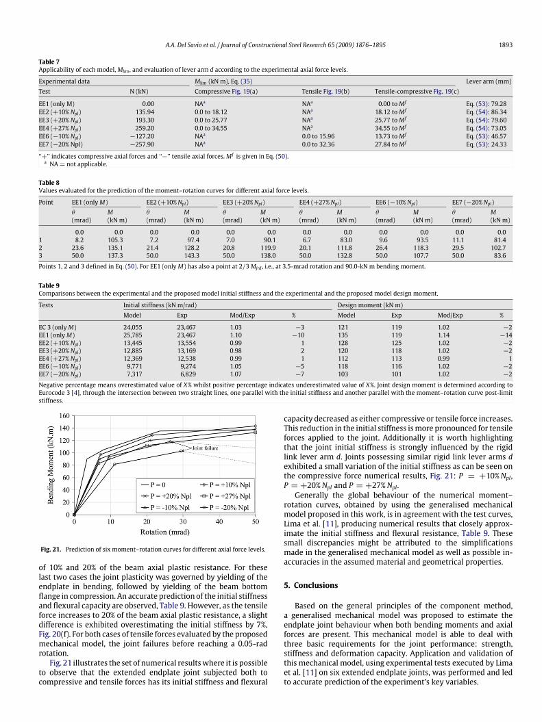
Fig. 21. Prediction of six moment–rotation curves for different axial force levels.
of 10% and 20% of the beam axial plastic resistance. For theselast two cases the joint plasticity was governed by yielding of theendplate in bending, followed by yielding of the beam bottomflange in compression. An accurate prediction of the initial stiffnessand flexural capacity are observed, Table 9. However, as the tensileforce increases to 20% of the beam axial plastic resistance, a slightdifference is exhibited overestimating the initial stiffness by 7%,Fig. 20(f). For both cases of tensile forces evaluated by the proposedmechanical model, the joint failures before reaching a 0.05-radrotation.Fig. 21 illustrates the set of numerical resultswhere it is possible
to observe that the extended endplate joint subjected both tocompressive and tensile forces has its initial stiffness and flexural
capacity decreased as either compressive or tensile force increases.This reduction in the initial stiffness ismore pronounced for tensileforces applied to the joint. Additionally it is worth highlightingthat the joint initial stiffness is strongly influenced by the rigidlink lever arm d. Joints possessing similar rigid link lever arms dexhibited a small variation of the initial stiffness as can be seen onthe compressive force numerical results, Fig. 21: P = +10%Npl,P = +20%Npl and P = +27%Npl.Generally the global behaviour of the numerical moment–
rotation curves, obtained by using the generalised mechanicalmodel proposed in this work, is in agreement with the test curves,Lima et al. [11], producing numerical results that closely approx-imate the initial stiffness and flexural resistance, Table 9. Thesesmall discrepancies might be attributed to the simplificationsmade in the generalised mechanical model as well as possible in-accuracies in the assumed material and geometrical properties.
5. Conclusions
Based on the general principles of the component method,a generalised mechanical model was proposed to estimate theendplate joint behaviour when both bending moments and axialforces are present. This mechanical model is able to deal withthree basic requirements for the joint performance: strength,stiffness and deformation capacity. Application and validation ofthis mechanical model, using experimental tests executed by Limaet al. [11] on six extended endplate joints, was performed and ledto accurate prediction of the experiment’s key variables.
1894 A.A. Del Savio et al. / Journal of Constructional Steel Research 65 (2009) 1876–1895
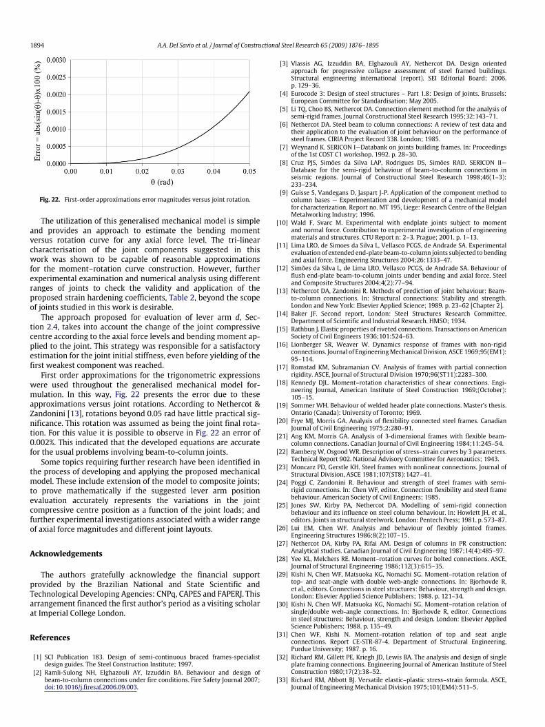
Fig. 22. First-order approximations error magnitudes versus joint rotation.
The utilization of this generalised mechanical model is simpleand provides an approach to estimate the bending momentversus rotation curve for any axial force level. The tri-linearcharacterisation of the joint components suggested in thiswork was shown to be capable of reasonable approximationsfor the moment–rotation curve construction. However, furtherexperimental examination and numerical analysis using differentranges of joints to check the validity and application of theproposed strain hardening coefficients, Table 2, beyond the scopeof joints studied in this work is desirable.The approach proposed for evaluation of lever arm d, Sec-
tion 2.4, takes into account the change of the joint compressivecentre according to the axial force levels and bending moment ap-plied to the joint. This strategy was responsible for a satisfactoryestimation for the joint initial stiffness, even before yielding of thefirst weakest component was reached.First order approximations for the trigonometric expressions
were used throughout the generalised mechanical model for-mulation. In this way, Fig. 22 presents the error due to theseapproximations versus joint rotations. According to Nethercot &Zandonini [13], rotations beyond 0.05 rad have little practical sig-nificance. This rotation was assumed as being the joint final rota-tion. For this value it is possible to observe in Fig. 22 an error of0.002%. This indicated that the developed equations are accuratefor the usual problems involving beam-to-column joints.Some topics requiring further research have been identified in
the process of developing and applying the proposed mechanicalmodel. These include extension of the model to composite joints;to prove mathematically if the suggested lever arm positionevaluation accurately represents the variations in the jointcompressive centre position as a function of the joint loads; andfurther experimental investigations associated with a wider rangeof axial force magnitudes and different joint layouts.
Acknowledgements
The authors gratefully acknowledge the financial supportprovided by the Brazilian National and State Scientific andTechnological Developing Agencies: CNPq, CAPES and FAPERJ. Thisarrangement financed the first author’s period as a visiting scholarat Imperial College London.
References
[1] SCI Publication 183. Design of semi-continuous braced frames-specialistdesign guides. The Steel Construction Institute; 1997.
[2] Ramli-Sulong NH, Elghazouli AY, Izzuddin BA. Behaviour and design ofbeam-to-column connections under fire conditions. Fire Safety Journal 2007;doi:10.1016/j.firesaf.2006.09.003.
[3] Vlassis AG, Izzuddin BA, Elghazouli AY, Nethercot DA. Design orientedapproach for progressive collapse assessment of steel framed buildings.Structural engineering international (report). SEI Editorial Board; 2006.p. 129–36.
[4] Eurocode 3: Design of steel structures – Part 1.8: Design of joints. Brussels:European Committee for Standardisation; May 2005.
[5] Li TQ, Choo BS, Nethercot DA. Connection element method for the analysis ofsemi-rigid frames. Journal Constructional Steel Research 1995;32:143–71.
[6] Nethercot DA. Steel beam to column connections: A review of test data andtheir application to the evaluation of joint behaviour on the performance ofsteel frames. CIRIA Project Record 338. London; 1985.
[7] Weynand K. SERICON I—Databank on joints building frames. In: Proceedingsof the 1st COST C1 workshop. 1992. p. 28–30.
[8] Cruz PJS, Simões da Silva LAP, Rodrigues DS, Simões RAD. SERICON II—Database for the semi-rigid behaviour of beam-to-column connections inseismic regions. Journal of Constructional Steel Research 1998;46(1–3):233–234.
[9] Guisse S, Vandegans D, Jaspart J-P. Application of the component method tocolumn bases — Experimentation and development of a mechanical modelfor characterization. Report no. MT 195, Liege: Research Centre of the BelgianMetalworking Industry; 1996.
[10] Wald F, Svarc M. Experimental with endplate joints subject to momentand normal force. Contribution to experimental investigation of engineeringmaterials and structures. CTU Report n: 2–3. Prague; 2001. p. 1–13.
[11] Lima LRO, de Simoes da Silva L, Vellasco PCGS, de Andrade SA. Experimentalevaluation of extended end-plate beam-to-column joints subjected to bendingand axial force. Engineering Structures 2004;26:1333–47.
[12] Simões da Silva L, de Lima LRO, Vellasco PCGS, de Andrade SA. Behaviour offlush end-plate beam-to-column joints under bending and axial force. Steeland Composite Structures 2004;4(2):77–94.
[13] Nethercot DA, Zandonini R. Methods of prediction of joint behaviour: Beam-to-column connections. In: Structural connections: Stability and strength.London and New York: Elsevier Applied Science; 1989. p. 23–62 [Chapter 2].
[14] Baker JF. Second report, London: Steel Structures Research Committee,Department of Scientific and Industrial Research. HMSO; 1934.
[15] Rathbun J. Elastic properties of riveted connections. Transactions on AmericanSociety of Civil Engineers 1936;101:524–63.
[16] Lionberger SR, Weaver W. Dynamics response of frames with non-rigidconnections. Journal of EngineeringMechanical Division, ASCE 1969;95(EM1):95–114.
[17] Romstad KM, Subramanian CV. Analysis of frames with partial connectionrigidity. ASCE, Journal of Structural Division 1970;96(ST11):2283–300.
[18] Kennedy DJL. Moment–rotation characteristics of shear connections. Engi-neering Journal, American Institute of Steel Construction 1969;(October):105–15.
[19] Sommer WH. Behaviour of welded header plate connections. Master’s thesis.Ontario (Canada): University of Toronto; 1969.
[20] Frye MJ, Morris GA. Analysis of flexibility connected steel frames. CanadianJournal of Civil Engineering 1975;2:280–91.
[21] Ang KM, Morris GA. Analysis of 3-dimensional frames with flexible beam-column connections. Canadian Journal of Civil Engineering 1984;11:245–54.
[22] Ramberg W, Osgood WR. Description of stress–strain curves by 3 parameters.Technical Report 902. National Advisory Committee for Aeronautics; 1943.
[23] Moncarz PD, Gerstle KH. Steel frames with nonlinear connections. Journal ofStructural Division, ASCE 1981;107(ST8):1427–41.
[24] Poggi C, Zandonini R. Behaviour and strength of steel frames with semi-rigid connections. In: Chen WF, editor. Connection flexibility and steel framebehaviour. American Society of Civil Engineers; 1985.
[25] Jones SW, Kirby PA, Nethercot DA. Modelling of semi-rigid connectionbehaviour and its influence on steel column behaviour. In: Howlett JH, et al.,editors. Joints in structural steelwork. London: Pentech Press; 1981. p. 573–87.
[26] Lui EM, Chen WF. Analysis and behaviour of flexibly jointed frames.Engineering Structures 1986;8(2):107–15.
[27] Nethercot DA, Kirby PA, Rifai AM. Design of columns in PR construction:Analytical studies. Canadian Journal of Civil Engineering 1987;14(4):485–97.
[28] Yee KL, Melchers RE. Moment–rotation curves for bolted connections. ASCE,Journal of Structural Engineering 1986;112(3):615–35.
[29] Kishi N, Chen WF, Matsuoka KG, Nomachi SG. Moment–rotation relation oftop- and seat-angle with double web-angle connections. In: Bjorhovde R,et al., editors. Connections in steel structures: Behaviour, strength and design.London: Elsevier Applied Science Publishers; 1988. p. 121–34.
[30] Kishi N, Chen WF, Matsuoka KG, Nomachi SG. Moment–rotation relation ofsingle/double web-angle connections. In: Bjorhovde R, editor. Connectionsin steel structures: Behaviour, strength and design. London: Elsevier AppliedScience Publishers; 1988. p. 135–49.
[31] Chen WF, Kishi N. Moment–rotation relation of top and seat angleconnections. Report CE-STR-87-4. Department of Structural Engineering,Purdue University; 1987. p. 16.
[32] Richard RM, Gillett PE, Kriegh JD, Lewis BA. The analysis and design of singleplate framing connections. Engineering Journal of American Institute of SteelConstruction 1980;17(2):38–52.
[33] Richard RM, Abbott BJ. Versatile elastic–plastic stress–strain formula. ASCE,Journal of Engineering Mechanical Division 1975;101(EM4):511–5.
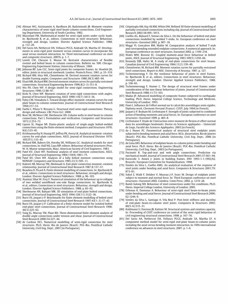
A.A. Del Savio et al. / Journal of Constructional Steel Research 65 (2009) 1876–1895 1895
[34] Altman WG, Azizinamini A, Bardburn JH, Radziminski JB. Moment–rotationcharacteristics of semi-rigid steel beam-column connections. Civil Engineer-ing Department, University of South Carolina; 1982.
[35] Mazzolani FM. Mathematical model for semi-rigid joints under cyclic loads.In: Bjorhovde R, et al., editors. Connections in steel structures: Behaviour,strength and design. London: Elsevier Applied Science Publisher; 1988.p. 112–20.
[36] Del Savio AA, Nethercot DA, Vellasco PCGS, Andrade SA, Martha LF. Develop-ments in semi-rigid joint moment versus rotation curves to incorporate theaxial versus moment interaction. In: Third international conference on steeland composite structures. 2007b. p. 1–7.
[37] Lewitt CW, Chesson E, Munse W. Restraint characteristics of flexibleriveted and bolted beam to column connections. Bulletin no. 500. Chicago:Engineering Experiment Station, University of Illinois; 1969.
[38] Johnson RP, Law CLC. Semi-rigid joints for composite frames. In: Howlett JH,editor. Joints in structural steelwork. London: Pentech Press; 1981. p. 33–319.
[39] Richard RM, Hsia WK, Chmielowiec M. Derived moment rotation curves fordouble framing angles. Computers and Structures 1988;30(3):485–94.
[40] ElsatiMK, RichardRM.Derivedmoment rotation curves for partially restrainedconnections. Structural Engineering Review 1996;8(2–3):151–8.
[41] Wu FH, Chen WF. A design model for semi-rigid connections. EngineeringStructures 1990;12:88–97.
[42] Kishi N, Chen WF. Moment–rotation of semi-rigid connections with angles.Journal of Structural Engineering, ASCE 1990;116(7):1813–34.
[43] Foley CM, Vinnakota S. Toward design office moment–rotation curves for endplate beam-to-column connections. Journal of Constructional Steel Research1994;217–53.
[44] Faella C, Piluso V, Rizzano G. Structural steel semi-rigid connections: Theory,design and software. CRC Press LLC; 2000.
[45] Bose SK, McNeice GM, Sherbourne AN. Column webs in steel beam to columnconnections. Part I, Formulation and verification. Computers and Structures1972;2:253–72.
[46] Lipson SL, Hague MI. Elasto-plastic analysis of single-angle bolted-weldedconnections using the finite elementmethod. Computers and Structures 1978;9(6):533–45.
[47] KrishnamurthyN, HuangHT, Jeffrey PK, Avery LK. Analyticalmoment–rotationcurves for end-plate connections. ASCE, Journal of Structural Division 1979;105(ST1):133–45.
[48] Richard RM, Rabern DA, Hornby DE, Williams GC. Analytical models for steelconnections. In: HallWJ, GausMP, editors. Behaviour ofmetal structures (Proc.W. H. Munse symposium, May). American Society of Civil Engineers; 1983.
[49] Patel KV, Chen WF. Nonlinear analysis of steel moment connections. ASCE,Journal of Structural Engineering 1984;110(8):1861–75.
[50] Patel KV, Chen WF. Analysis of a fully bolted moment connection usingNONSAP. Computers and Structures 1985;21(3):505–11.
[51] Kukreti AR, Murray TM, Abolmaali A. End-plate connection moment–rotationrelationship. Journal of Constructional Steel Research 1987;8:137–57.
[52] Beaulieu D, Picard A. Finite elementmodelling of connections. In: Bjorhovde R,et al., editors. Connections in steel structures: Behaviour, strength and design.London: Elsevier Applied Science Publishers; 1988. p. 96–103.
[53] Atamiaz Sibai W, Frey F. Numerical simulation of the behaviour up to collapseof two welded unstiffened one-side flange connections. In: Bjorhovde R,et al., editors. Connections in steel structures: Behaviour, strength and design.London: Elsevier Applied Science Publishers; 1988. p. 85–92.
[54] Sherbourne AN, Bahaari MR. 3D simulation of end-plate bolted connections.Journal of Structural Engineering, ASCE 1994;120(11):3122–36.
[55] Bursi OS, Jaspart J-P. Benchmarks for finite element modelling of bolted steelconnections. Journal of Constructional Steel Research 1997;43(1–3):17–42.
[56] Bursi OS, Jaspart J-P. Calibration of a finite element model for isolated boltedend-plate steel connections. Journal of Constructional Steel Research 1998;44(3):225–62.
[57] Yang JG, Murray TM, Plaut RH. Three-dimensional finite element analysis ofdouble angle connections under tension and shear. Journal of ConstructionalSteel Research 2000;54:227–44.
[58] de Cardoso DCL. Numerical modelling of semi-rigid connection for steelstructures. Ph.D. thesis. Rio de Janeiro (Brazil): PUC-Rio, Pontifical CatholicUniversity, Civil Eng. Dept.; 2001 [in Portuguese].
[59] Citipitioglu AM,Haj-Ali RM,White DW. Refined 3D finite elementmodelling ofpartially-restrained connections including slip. Journal of Constructional SteelResearch 2002;58:995–1013.
[60] Coelho AG, Bijlaard F, Simoes da Silva L. On the behaviour of bolted end plateconnections modelled by welded T-stubs. In: European conference on steelstructures—Eurosteel 2002. p. 907–18.
[61] Maggi YI, Goncalves RM, Malite M. Comparative analysis of bolted T-stuband corresponding extended endplate connections: A numerical approach. In:European conference on steel structures. Eurosteel 2002. p. 1199–218.
[62] Wales MW, Rossow EC. Coupled moment-axial force behaviour in boltedjoints. ASCE, Journal of Structural Engineering 1983;109(5):1250–66.
[63] Kennedy DJR, Hafez M. A study of end-plate connections for steel beams.Canadian Journal of Civil Engineering 1984;11(2):139–49.
[64] Chmielowiec M, Richard RM. Moment rotation curves for partially restrainedsteel connections. Report to AISC. University of Arizona; 1987. p. 127.
[65] Tschemmernegg F. On the nonlinear behaviour of joints in steel frames.In: Bjorhovde R, et al., editors. Connections in steel structures: Behaviour,strength and design. London: Elsevier Applied Science Publishers; 1988.p. 158–65.
[66] Tschemmernegg F, Humer C. The design of structural steel frames underconsideration of the non-linear behaviour of joints. Journal of ConstructionalSteel Research 1988;11:73–103.
[67] Madas JP. Advanced modelling of composite frames subjected to earthquakeloading. Ph.D. thesis. Imperial College Science, Technology and Medicine,University of London; 1993.
[68] Finet L. Influence de l’effort normal sur le calcul des assemblages semi-rigides.Diploma work. Clermont-Ferrand (France): CUST; July 1994 [in French].
[69] Jaspart J-P, BrahamM, Cerfontaine F. Strength of joints subjected to combinedaction of bending moments and axial forces. In: European conference on steelstructures—Eurosteel 1999. p. 465–8.
[70] Cerfontaine F. Etude de l’interaction entre moment de flexion et effort normaldans les assemblages boulonnés. Doctor en Sciences appliquées – Universitéde Liege, Faculté des Sciences Appliquées; 2003 [in French].
[71] da L Nunes PC. Parametrical analysis of structural steel endplate jointssubjected to bendingmoment and axial force.M.Sc. dissertation. Rio de Janeiro(Brazil): PUC-Rio, Pontifical Catholic University, Civil Eng. Dept.; 2006 [inPortuguese].
[72] de Lima LRO. Behaviour of endplate beam-to-column joints under bending andaxial force. Ph.D. thesis. Rio de Janeiro (Brazil): PUC-Rio, Pontifical CatholicUniversity, Civil Eng. Dept.; 2003 [in Portuguese].
[73] Pucinotti R. Top-and-seat and web angle connections: Prediction viamechanical model. Journal of Constructional Steel Research 2001;57:661–94.
[74] Eurocode 3. Annex J: Joints in building frames. ENV 1993-1-1:1992/A2.Brussels: European Committee for Standardisation; 1998.
[75] Simões da Silva L, Coelho AMG. An analytical evaluation of the response ofsteel joints under bending and axial force. Computers & Structures 2001;79:873–81.
[76] Sokol Z, Wald F, Delabre V, Muzeau J-P, Svarc M. Design of endplate jointssubject to moment and normal force. In: Third European conference on steelstructures—Eurosteel 2002. Coimbra: Cmm Press; 2002. p. 1219–28.
[77] Ramli-Sulong NH. Behaviour of steel connections under fire conditions. Ph.D.thesis. Imperial College London, University of London; 2005.
[78] Urbonas K, Daniunas A. Behaviour of semi-rigid steel beam-to-beam jointsunder bending and axial forces. Journal of Constructional Steel Research 2006;62:1244–9.
[79] Simões da Silva L, Santiago A, Vila Real P. Post-limit stiffness and ductilityof end-plate beam-to-column steel joints. Computers & Structures 2002;80(5–6):515–31.
[80] Kuhlmann U, Davison JB, Kattner M. Structural systems and rotation capacity.In: Proceeding of COST conference on control of the semi-rigid behaviour ofcivil engineering structural connections. 1998. p. 167–76.
[81] Del Savio AA, Nethercot DA, Vellasco PCGS, Andrade SA, Martha LF. Acomponent method model for semi-rigid end-plate beam-to-column jointsincluding the axial versus bending moment interaction. In: Fifth internationalconference on advances in steel structures. 2007. p. 1–6.