Embed Size (px)
Citation preview
Generalised method of moments estimation ofstructural mean models
Tom Palmer1,2 Roger Harbord2 Paul Clarke3
Frank Windmeijer3,4,5
1. MRC Centre for Causal Analyses in Translational Epidemiology2. School of Social and Community Medicine, University of Bristol
3. CMPO, University of Bristol4. Department of Economics, University of Bristol, UK
5. CEMMAP/IFS, London
15 September 2011
Centre for Causal
Analyses in Translational
Epidemiology
Outline
Generalised method of moments estimation of structural meanmodels . . . using instrumental variables
I Introduction to Mendelian randomization exampleI Multiplicative structural mean model (MSMM)
I G-estimation, identification, gmm syntax, example
I (double) Logistic SMMI gmm multiple equation syntax, example
I Summary
I MSMM: local risk ratios
1 / 20
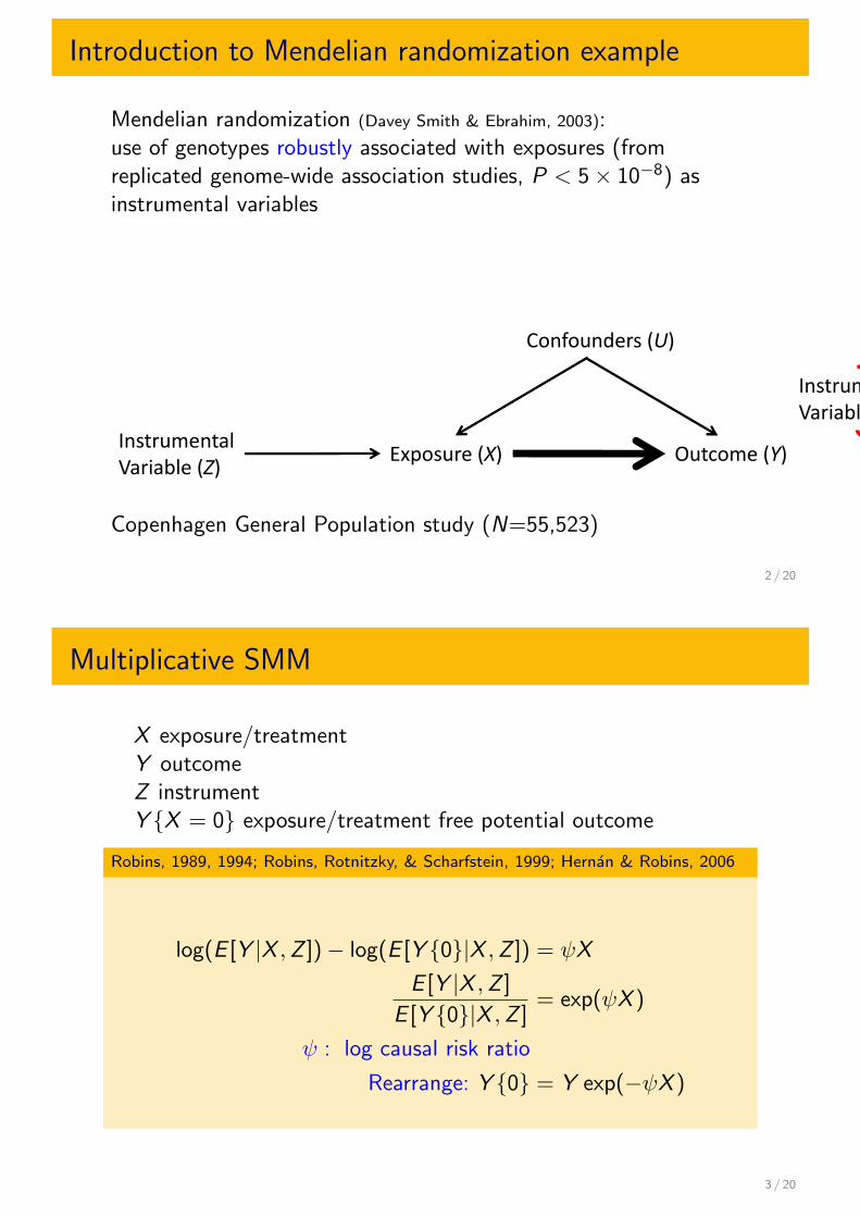
Introduction to Mendelian randomization example
Mendelian randomization (Davey Smith & Ebrahim, 2003):use of genotypes robustly associated with exposures (fromreplicated genome-wide association studies, P < 5× 10⁻⁸) asinstrumental variables
InstrumentalVariable (Z)
Exposure (X) Outcome (Y)
Confounders (U)
InstrumentalVariable (Z)
Exposure (X) Outcome (Y)
Confounders (U)
A1
A2
A3 FTO, MC4R genotypes (Z)
Overweight(BMI>25) (X)
Hypertension (Y)
Confounders (U)
Copenhagen General Population study (N=55,523)
2 / 20
Multiplicative SMM
X exposure/treatmentY outcomeZ instrumentY {X = 0} exposure/treatment free potential outcome
Robins, 1989, 1994; Robins, Rotnitzky, & Scharfstein, 1999; Hernan & Robins, 2006
log(E [Y |X ,Z ])− log(E [Y {0}|X ,Z ]) = ψX
E [Y |X ,Z ]
E [Y {0}|X ,Z ]= exp(ψX )
ψ : log causal risk ratio
Rearrange: Y {0} = Y exp(−ψX )
3 / 20
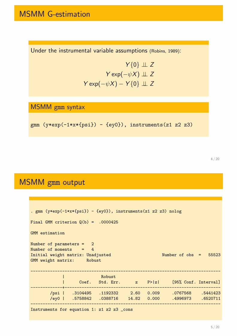
MSMM G-estimation
Under the instrumental variable assumptions (Robins, 1989):
Y {0} ⊥⊥ Z
Y exp(−ψX ) ⊥⊥ Z
Y exp(−ψX )− Y {0} ⊥⊥ Z
MSMM gmm syntax
gmm (y*exp(-1*x*{psi}) - {ey0}), instruments(z1 z2 z3)
4 / 20
MSMM gmm output
. gmm (y*exp(-1*x*{psi}) - {ey0}), instruments(z1 z2 z3) nolog
Final GMM criterion Q(b) = .0000425
GMM estimation
Number of parameters = 2
Number of moments = 4
Initial weight matrix: Unadjusted Number of obs = 55523
GMM weight matrix: Robust
------------------------------------------------------------------------------
| Robust
| Coef. Std. Err. z P>|z| [95% Conf. Interval]
-------------+----------------------------------------------------------------
/psi | .3104495 .1192332 2.60 0.009 .0767568 .5441423
/ey0 | .5758842 .0388716 14.82 0.000 .4996973 .6520711
------------------------------------------------------------------------------
Instruments for equation 1: z1 z2 z3 _cons
5 / 20
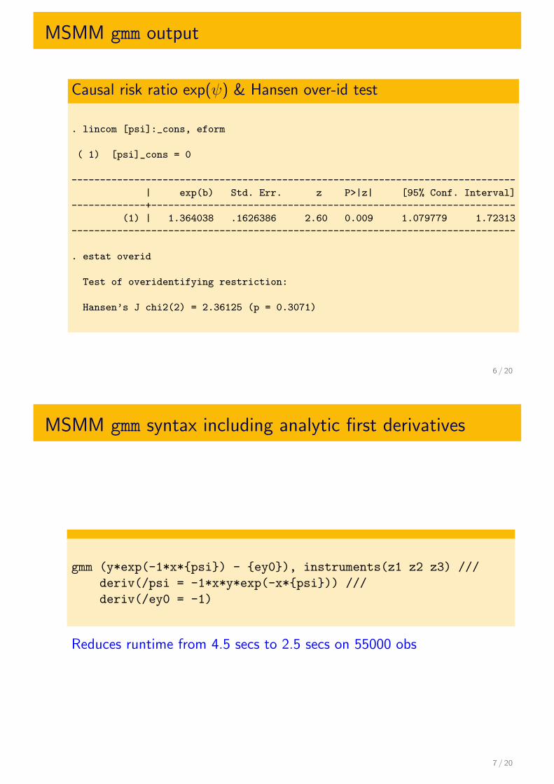
MSMM gmm output
Causal risk ratio exp(ψ) & Hansen over-id test
. lincom [psi]:_cons, eform
( 1) [psi]_cons = 0
------------------------------------------------------------------------------
| exp(b) Std. Err. z P>|z| [95% Conf. Interval]
-------------+----------------------------------------------------------------
(1) | 1.364038 .1626386 2.60 0.009 1.079779 1.72313
------------------------------------------------------------------------------
. estat overid
Test of overidentifying restriction:
Hansen’s J chi2(2) = 2.36125 (p = 0.3071)
6 / 20
MSMM gmm syntax including analytic first derivatives
gmm (y*exp(-1*x*{psi}) - {ey0}), instruments(z1 z2 z3) ///
deriv(/psi = -1*x*y*exp(-x*{psi})) ///
deriv(/ey0 = -1)
Reduces runtime from 4.5 secs to 2.5 secs on 55000 obs
7 / 20
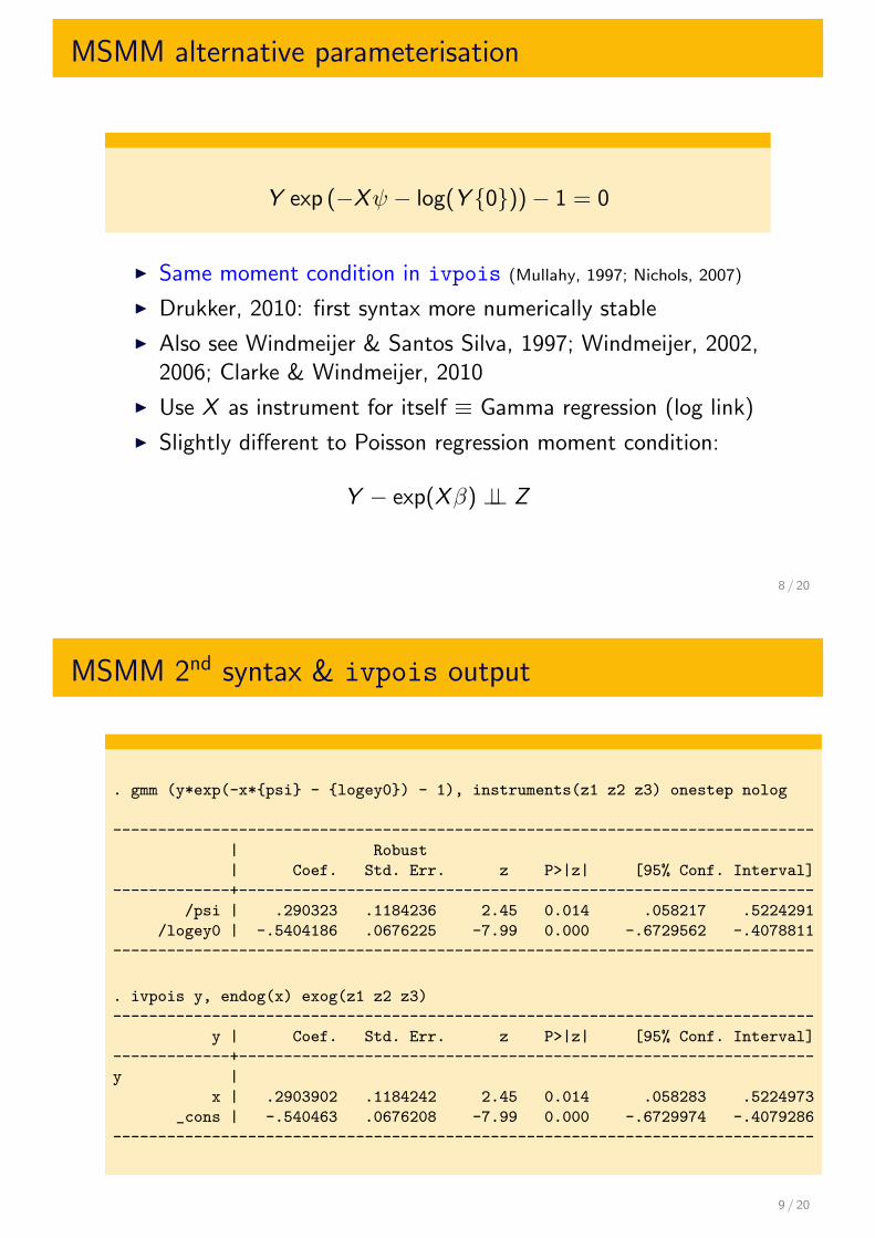
MSMM alternative parameterisation
Y exp (−Xψ − log(Y {0}))− 1 = 0
I Same moment condition in ivpois (Mullahy, 1997; Nichols, 2007)
I Drukker, 2010: first syntax more numerically stable
I Also see Windmeijer & Santos Silva, 1997; Windmeijer, 2002,2006; Clarke & Windmeijer, 2010
I Use X as instrument for itself ≡ Gamma regression (log link)
I Slightly different to Poisson regression moment condition:
Y − exp(Xβ) ⊥⊥ Z
8 / 20
MSMM 2nd syntax & ivpois output
. gmm (y*exp(-x*{psi} - {logey0}) - 1), instruments(z1 z2 z3) onestep nolog
------------------------------------------------------------------------------
| Robust
| Coef. Std. Err. z P>|z| [95% Conf. Interval]
-------------+----------------------------------------------------------------
/psi | .290323 .1184236 2.45 0.014 .058217 .5224291
/logey0 | -.5404186 .0676225 -7.99 0.000 -.6729562 -.4078811
------------------------------------------------------------------------------
. ivpois y, endog(x) exog(z1 z2 z3)
------------------------------------------------------------------------------
y | Coef. Std. Err. z P>|z| [95% Conf. Interval]
-------------+----------------------------------------------------------------
y |
x | .2903902 .1184242 2.45 0.014 .058283 .5224973
_cons | -.540463 .0676208 -7.99 0.000 -.6729974 -.4079286
------------------------------------------------------------------------------
9 / 20
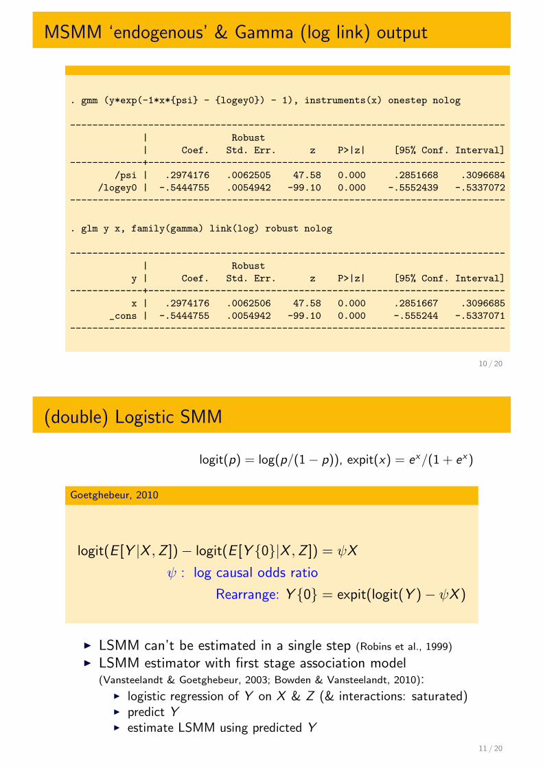
MSMM ‘endogenous’ & Gamma (log link) output
. gmm (y*exp(-1*x*{psi} - {logey0}) - 1), instruments(x) onestep nolog
------------------------------------------------------------------------------
| Robust
| Coef. Std. Err. z P>|z| [95% Conf. Interval]
-------------+----------------------------------------------------------------
/psi | .2974176 .0062505 47.58 0.000 .2851668 .3096684
/logey0 | -.5444755 .0054942 -99.10 0.000 -.5552439 -.5337072
------------------------------------------------------------------------------
. glm y x, family(gamma) link(log) robust nolog
------------------------------------------------------------------------------
| Robust
y | Coef. Std. Err. z P>|z| [95% Conf. Interval]
-------------+----------------------------------------------------------------
x | .2974176 .0062506 47.58 0.000 .2851667 .3096685
_cons | -.5444755 .0054942 -99.10 0.000 -.555244 -.5337071
------------------------------------------------------------------------------
10 / 20
(double) Logistic SMM
logit(p) = log(p/(1− p)), expit(x) = ex/(1 + ex)
Goetghebeur, 2010
logit(E [Y |X ,Z ])− logit(E [Y {0}|X ,Z ]) = ψX
ψ : log causal odds ratio
Rearrange: Y {0} = expit(logit(Y )− ψX )
I LSMM can’t be estimated in a single step (Robins et al., 1999)
I LSMM estimator with first stage association model(Vansteelandt & Goetghebeur, 2003; Bowden & Vansteelandt, 2010):
I logistic regression of Y on X & Z (& interactions: saturated)I predict YI estimate LSMM using predicted Y
11 / 20
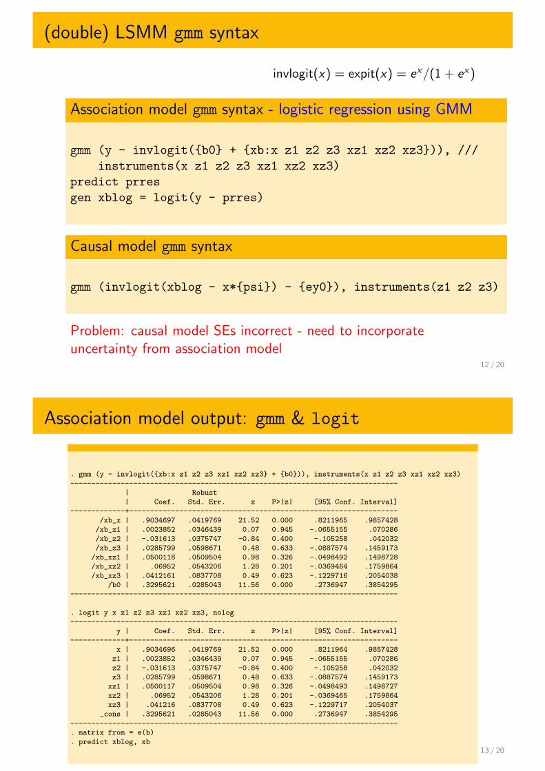
(double) LSMM gmm syntax
invlogit(x) = expit(x) = ex/(1 + ex)
Association model gmm syntax - logistic regression using GMM
gmm (y - invlogit({b0} + {xb:x z1 z2 z3 xz1 xz2 xz3})), ///
instruments(x z1 z2 z3 xz1 xz2 xz3)
predict prres
gen xblog = logit(y - prres)
Causal model gmm syntax
gmm (invlogit(xblog - x*{psi}) - {ey0}), instruments(z1 z2 z3)
Problem: causal model SEs incorrect - need to incorporateuncertainty from association model
12 / 20
Association model output: gmm & logit
. gmm (y - invlogit({xb:x z1 z2 z3 xz1 xz2 xz3} + {b0})), instruments(x z1 z2 z3 xz1 xz2 xz3)
------------------------------------------------------------------------------
| Robust
| Coef. Std. Err. z P>|z| [95% Conf. Interval]
-------------+----------------------------------------------------------------
/xb_x | .9034697 .0419769 21.52 0.000 .8211965 .9857428
/xb_z1 | .0023852 .0346439 0.07 0.945 -.0655155 .070286
/xb_z2 | -.031613 .0375747 -0.84 0.400 -.105258 .042032
/xb_z3 | .0285799 .0598671 0.48 0.633 -.0887574 .1459173
/xb_xz1 | .0500118 .0509504 0.98 0.326 -.0498492 .1498728
/xb_xz2 | .06952 .0543206 1.28 0.201 -.0369464 .1759864
/xb_xz3 | .0412161 .0837708 0.49 0.623 -.1229716 .2054038
/b0 | .3295621 .0285043 11.56 0.000 .2736947 .3854295
------------------------------------------------------------------------------
. logit y x z1 z2 z3 xz1 xz2 xz3, nolog
------------------------------------------------------------------------------
y | Coef. Std. Err. z P>|z| [95% Conf. Interval]
-------------+----------------------------------------------------------------
x | .9034696 .0419769 21.52 0.000 .8211964 .9857428
z1 | .0023852 .0346439 0.07 0.945 -.0655155 .070286
z2 | -.031613 .0375747 -0.84 0.400 -.105258 .042032
z3 | .0285799 .0598671 0.48 0.633 -.0887574 .1459173
xz1 | .0500117 .0509504 0.98 0.326 -.0498493 .1498727
xz2 | .06952 .0543206 1.28 0.201 -.0369465 .1759864
xz3 | .041216 .0837708 0.49 0.623 -.1229717 .2054037
_cons | .3295621 .0285043 11.56 0.000 .2736947 .3854295
------------------------------------------------------------------------------
. matrix from = e(b)
. predict xblog, xb13 / 20
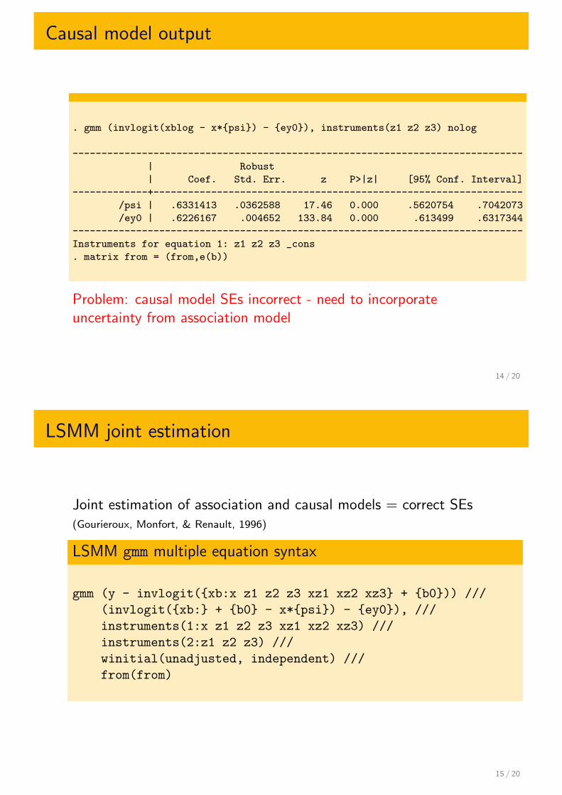
Causal model output
. gmm (invlogit(xblog - x*{psi}) - {ey0}), instruments(z1 z2 z3) nolog
------------------------------------------------------------------------------
| Robust
| Coef. Std. Err. z P>|z| [95% Conf. Interval]
-------------+----------------------------------------------------------------
/psi | .6331413 .0362588 17.46 0.000 .5620754 .7042073
/ey0 | .6226167 .004652 133.84 0.000 .613499 .6317344
------------------------------------------------------------------------------
Instruments for equation 1: z1 z2 z3 _cons
. matrix from = (from,e(b))
Problem: causal model SEs incorrect - need to incorporateuncertainty from association model
14 / 20
LSMM joint estimation
Joint estimation of association and causal models = correct SEs(Gourieroux, Monfort, & Renault, 1996)
LSMM gmm multiple equation syntax
gmm (y - invlogit({xb:x z1 z2 z3 xz1 xz2 xz3} + {b0})) ///
(invlogit({xb:} + {b0} - x*{psi}) - {ey0}), ///
instruments(1:x z1 z2 z3 xz1 xz2 xz3) ///
instruments(2:z1 z2 z3) ///
winitial(unadjusted, independent) ///
from(from)
15 / 20
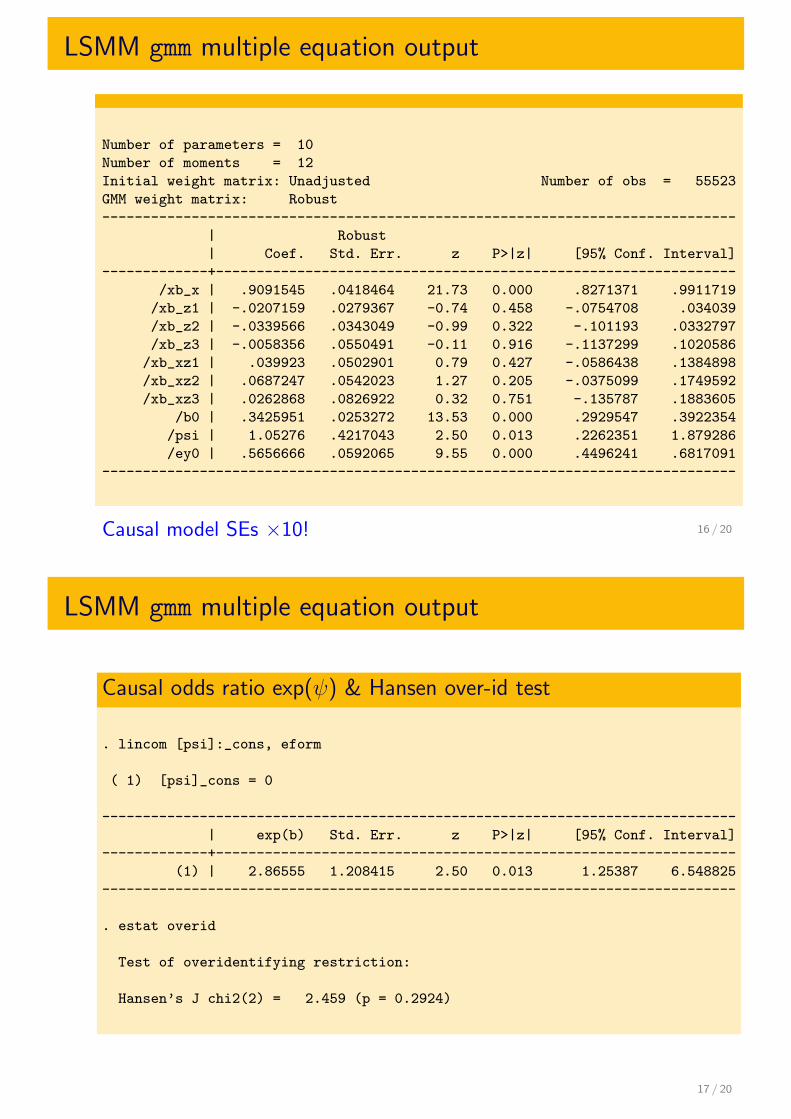
LSMM gmm multiple equation output
Number of parameters = 10
Number of moments = 12
Initial weight matrix: Unadjusted Number of obs = 55523
GMM weight matrix: Robust
------------------------------------------------------------------------------
| Robust
| Coef. Std. Err. z P>|z| [95% Conf. Interval]
-------------+----------------------------------------------------------------
/xb_x | .9091545 .0418464 21.73 0.000 .8271371 .9911719
/xb_z1 | -.0207159 .0279367 -0.74 0.458 -.0754708 .034039
/xb_z2 | -.0339566 .0343049 -0.99 0.322 -.101193 .0332797
/xb_z3 | -.0058356 .0550491 -0.11 0.916 -.1137299 .1020586
/xb_xz1 | .039923 .0502901 0.79 0.427 -.0586438 .1384898
/xb_xz2 | .0687247 .0542023 1.27 0.205 -.0375099 .1749592
/xb_xz3 | .0262868 .0826922 0.32 0.751 -.135787 .1883605
/b0 | .3425951 .0253272 13.53 0.000 .2929547 .3922354
/psi | 1.05276 .4217043 2.50 0.013 .2262351 1.879286
/ey0 | .5656666 .0592065 9.55 0.000 .4496241 .6817091
------------------------------------------------------------------------------
Causal model SEs ×10! 16 / 20
LSMM gmm multiple equation output
Causal odds ratio exp(ψ) & Hansen over-id test
. lincom [psi]:_cons, eform
( 1) [psi]_cons = 0
------------------------------------------------------------------------------
| exp(b) Std. Err. z P>|z| [95% Conf. Interval]
-------------+----------------------------------------------------------------
(1) | 2.86555 1.208415 2.50 0.013 1.25387 6.548825
------------------------------------------------------------------------------
. estat overid
Test of overidentifying restriction:
Hansen’s J chi2(2) = 2.459 (p = 0.2924)
17 / 20
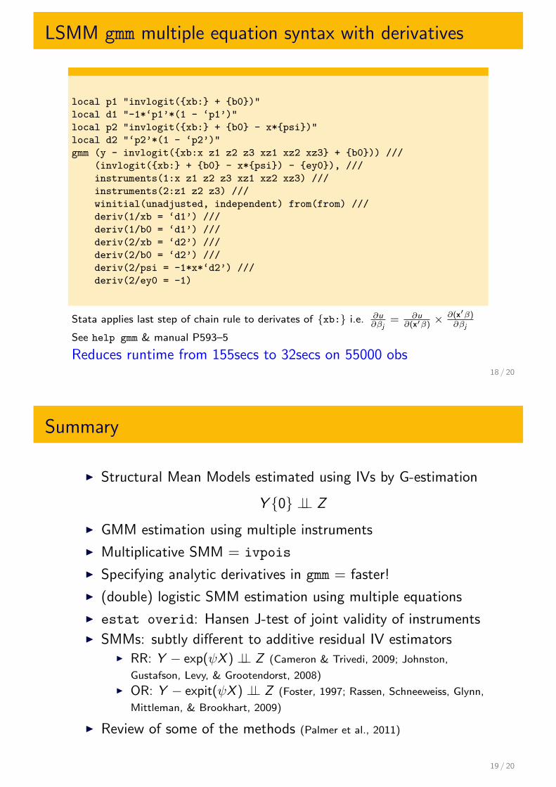
LSMM gmm multiple equation syntax with derivatives
local p1 "invlogit({xb:} + {b0})"
local d1 "-1*‘p1’*(1 - ‘p1’)"
local p2 "invlogit({xb:} + {b0} - x*{psi})"
local d2 "‘p2’*(1 - ‘p2’)"
gmm (y - invlogit({xb:x z1 z2 z3 xz1 xz2 xz3} + {b0})) ///
(invlogit({xb:} + {b0} - x*{psi}) - {ey0}), ///
instruments(1:x z1 z2 z3 xz1 xz2 xz3) ///
instruments(2:z1 z2 z3) ///
winitial(unadjusted, independent) from(from) ///
deriv(1/xb = ‘d1’) ///
deriv(1/b0 = ‘d1’) ///
deriv(2/xb = ‘d2’) ///
deriv(2/b0 = ‘d2’) ///
deriv(2/psi = -1*x*‘d2’) ///
deriv(2/ey0 = -1)
Stata applies last step of chain rule to derivates of {xb:} i.e. ∂u∂βj
= ∂u∂(x′β)
× ∂(x′β)∂βj
See help gmm & manual P593–5
Reduces runtime from 155secs to 32secs on 55000 obs18 / 20
Summary
I Structural Mean Models estimated using IVs by G-estimation
Y {0} ⊥⊥ Z
I GMM estimation using multiple instruments
I Multiplicative SMM = ivpois
I Specifying analytic derivatives in gmm = faster!
I (double) logistic SMM estimation using multiple equations
I estat overid: Hansen J-test of joint validity of instrumentsI SMMs: subtly different to additive residual IV estimators
I RR: Y − exp(ψX ) ⊥⊥ Z (Cameron & Trivedi, 2009; Johnston,
Gustafson, Levy, & Grootendorst, 2008)
I OR: Y − expit(ψX ) ⊥⊥ Z (Foster, 1997; Rassen, Schneeweiss, Glynn,
Mittleman, & Brookhart, 2009)
I Review of some of the methods (Palmer et al., 2011)
19 / 20
Acknowledgements
I MRC Collaborative grant G0601625
I MRC CAiTE Centre grant G0600705
I ESRC grant RES-060-23-0011
I With thanks to Nuala Sheehan, Vanessa Didelez, DebbieLawlor, Jonathan Sterne, George Davey Smith, Sha Meng,Neil Davies, Nic Timpson, Borge Nordestgaard.
References I
Bowden, J., & Vansteelandt, S. (2010). Mendelian randomisation analysis ofcase-control data using structural mean models. Statistics in Medicine. (inpress)
Cameron, A. C., & Trivedi, P. K. (2009). Microeconometrics using stata. CollegeStation, Texas: Stata Press.
Clarke, P. S., & Windmeijer, F. (2010). Identification of causal effects on binaryoutcomes using structural mean models. Biostatistics, 11(4), 756–770.
Davey Smith, G., & Ebrahim, S. (2003). ‘Mendelian randomization’: can geneticepidemiology contribute to understanding environmental determinants ofdisease. International Journal of Epidemiology, 32, 1–22.
Drukker, D. (2010). An introduction to GMM estimation using Stata. In Germanstata users group meeting. Berlin.
Foster, E. M. (1997). Instrumental variables for logistic regression: an illustration.Social Science Research, 26, 487–504.
Goetghebeur, E. (2010). Commentary: To cause or not to cause confusion vstransparency with Mendelian Randomization. International Journal ofEpidemiology, 39(3), 918–920.
Gourieroux, C., Monfort, A., & Renault, E. (1996). Two-stage generalized momentmethod with applications to regressions with heteroscedasticity of unknownform. Journal of Statistical Planning and Inference, 50(1), 37–63.
Hernan, M. A., & Robins, J. M. (2006). Instruments for Causal Inference. AnEpidemiologist’s Dream? Epidemiology, 17, 360–372.
References II
Imbens, G. W., & Angrist, J. D. (1994). Identification and Estimation of LocalAverage Treatment Effects. Econometrica, 62, 467–467.
Johnston, K. M., Gustafson, P., Levy, A. R., & Grootendorst, P. (2008). Use ofinstrumental variables in the analysis of generalized linear models in thepresence of unmeasured confounding with applications to epidemiologicalresearch. Statistics in Medicine, 27, 1539–1556.
Mullahy, J. (1997). Instrumental–variable estimation of count data models:Applications to models of cigarette smoking behaviour. The Review ofEconomics and Statistics, 79(4), 568–593.
Nichols, A. (2007). ivpois: Stata module for IV/GMM Poisson regression. StatisticalSoftware Components, Boston College Department of Economics. (available athttp://ideas.repec.org/c/boc/bocode/s456890.html)
Palmer, T. M., Sterne, J. A. C., Harbord, R. M., Lawlor, D. A., Sheehan, N. A.,Meng, S., et al. (2011). Instrumental variable estimation of causal risk ratiosand causal odds ratios in mendelian randomization analyses. American Journalof Epidemiology.
Rassen, J. A., Schneeweiss, S., Glynn, R. J., Mittleman, M. A., & Brookhart, M. A.(2009). Instrumental Variable Analysis for Estimation of Treatment EffectsWith Dichotomous Outcomes. American Journal of Epidemiology, 169(3),273–284.
References III
Robins, J. M. (1989). Health services research methodology: A focus on aids. InL. Sechrest, H. Freeman, & A. Mulley (Eds.), (chap. The analysis ofrandomized and non-randomized AIDS treatment trials using a new approachto causal inference in longitudinal studies). Washington DC, US: US PublicHealth Service.
Robins, J. M. (1994). Correcting for non-compliance in randomized trials usingstructural nested mean models. Communications in Statistics: Theory andMethods, 23(8), 2379–2412.
Robins, J. M., Rotnitzky, A., & Scharfstein, D. O. (1999). Statistical models inepidemiology: The environment and clinical trials. In M. E. Halloran &D. Berry (Eds.), (pp. 1–92). New York, US: Springer.
Vansteelandt, S., & Goetghebeur, E. (2003). Causal inference with generalizedstructural mean models. Journal of the Royal Statistical Society: Series B,65(4), 817–835.
Windmeijer, F. (2002). ExpEnd, A Gauss program for non-linear GMM estimation ofexponential models with endogenous regressors for cross section and paneldata (Tech. Rep.). Centre for Microdata Methods and Practice.
Windmeijer, F. (2006). GMM for panel count data models (Bristol EconomicsDiscussion Papers No. 06/591). Department of Economics, University ofBristol, UK. Available fromhttp://ideas.repec.org/p/bri/uobdis/06-591.html
References IV
Windmeijer, F., & Santos Silva, J. (1997). Endogeneity in Count Data Models: AnApplication to Demand for Health Care. Journal of Applied Econometrics,12(3), 281–294.
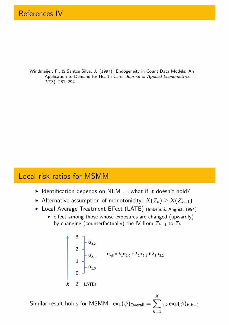
Local risk ratios for MSMM
I Identification depends on NEM . . . what if it doesn’t hold?
I Alternative assumption of monotonicity: X (Zk) ≥ X (Zk−1)I Local Average Treatment Effect (LATE) (Imbens & Angrist, 1994)
I effect among those whose exposures are changed (upwardly)by changing (counterfactually) the IV from Zk−1 to Zk
X$ Z$
3)
2
1
0
α3,2)
α2,1)
α1,0)
αAll)=)λ1α1,0)+)λ2α2,1)+)λ3α3,2)
LATEs)
Similar result holds for MSMM: exp(ψ)Overall =K∑
k=1
τk exp(ψ)k,k−1
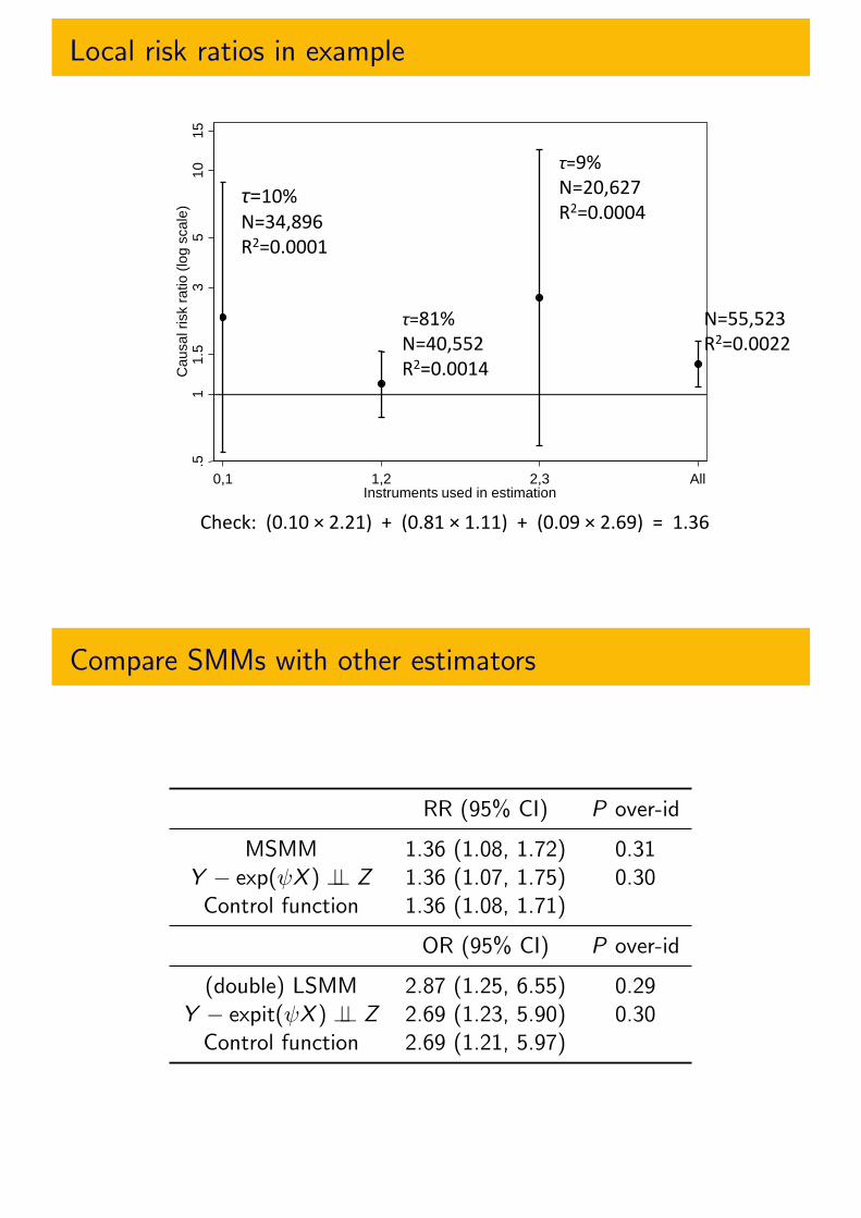
Local risk ratios in example
.51
1.5
35
10
15
Ca
usa
l ri
sk r
atio
(lo
g s
ca
le)
0,1 1,2 2,3 AllInstruments used in estimation
Check: (0.10 × 2.21) + (0.81 × 1.11) + (0.09 × 2.69) = 1.36
N=55,523R2=0.0022
τ=10%N=34,896R2=0.0001
τ=9%N=20,627R2=0.0004
τ=81%N=40,552R2=0.0014
Compare SMMs with other estimators
RR (95% CI) P over-id
MSMM 1.36 (1.08, 1.72) 0.31Y − exp(ψX ) ⊥⊥ Z 1.36 (1.07, 1.75) 0.30
Control function 1.36 (1.08, 1.71)
OR (95% CI) P over-id
(double) LSMM 2.87 (1.25, 6.55) 0.29Y − expit(ψX ) ⊥⊥ Z 2.69 (1.23, 5.90) 0.30
Control function 2.69 (1.21, 5.97)