Embed Size (px)
Citation preview
Generalized Best-First Search Strategies and the Optimality of A*
RINA DECHTER AND JUDEA PEARL
University of California, Los Angeles, California
Abstract. This paper reports several properties of heuristic best-first search strategies whose scoring functionsfdepend on all the information available from each candidate path, not merely on the current cost g and the estimated completion cost h. It is shown that several known properties of A* retain their form (with the minmax offplaying the role of the optimal cost), which helps establish general tests of admissibility and general conditions for node expansion for these strategies. On the basis of this framework the computational optimality of A*, in the sense of never expanding a node that can be skipped by some other algorithm having access to the same heuristic information that A* uses, is examined. A hierarchy of four optimality types is defined and three classes of algorithms and four domains of problem instances are considered. Computational performances relative to these algorithms and domains are appraised. For each class-domain combination, we then identify the strongest type of optimality that exists and the algorithm for achieving it. The main results of this paper relate to the class of algorithms that, like A*, return optimal solutions (i.e., admissible) when all cost estimates are optimistic (i.e., h 5 h*). On this class, A* is shown to be not optimal and it is also shown that no optimal algorithm exists, but if the performance tests are confirmed to cases in which the estimates are also consistent, then A* is indeed optimal. Additionally, A* is also shown to be optimal over a subset of the latter class containing all best-first algorithms that are guided by path-dependent evaluation functions.
Categories and Subject Descriptors: 1.2.8 [Artificial Intelligence]: Problem Solving, Control Methods and Search-graph and tree search strategies
General Terms: Algorithms, Measurement, Performance, Theory
Additional Key Words and Phrases: Best-first strategies, branch and bound, heuristic search, shortest path algorithms
1. Introduction Of all search strategies used in problem solving, one of the most popular methods of exploiting heuristic information to cut down search time is the injiyrmed best- first strategy. The general philosophy of this strategy is to use the heuristic information to assess the “merit” latent in every candidate search avenue exposed during the search and then continue the exploration along the direction of highest merit. Formal descriptions of this strategy are usually given in the context of path- searching problems [ 161, a formulation that represents many combinatorial prob- lems, such as routing, scheduling, speech recognition, and scene analys.is.
Given a weighted directional graph G with a distinguished start node s and a set of goal nodes r, the optimal path problem is to find a least-cost path from s to any
This work was supported in part by the National Science Foundation under Grant MCS 81-14209. Authors’ address: Cognitive Systems Laboratory, Computer Science Department, University of Califor- nia, Los Angeles, CA 90024. Permission to copy without fee all or part of this material is granted provided that the copies are not made or distributed for direct commercial advantage, the ACM copyright notice and the title of the publication and its date appear, and notice is given that copying is by permission of the Association for Computing Machinery. To copy otherwise, or to republish, requires a fee and/or specific permission. 0 1985 ACM 0004-541 l/85/0700-0505 $00.75
Journal of the Association for Computing Machinery, Vol. 32, No. 3, July 1985, pp. 505-536.
506 R. DECHTER AND J. PEARL
member of r where the cost of the path may, in general, be an arbitrary function of the weights assigned to the nodes and branches along that path. A general best- first (GBF) strategy will pursue this problem by constructing a tree T of selected paths of G using the elementary operation of node expansion, that is, generating all successors of a given node. Starting with s, GBF will select for expansion that leaf node of T that features the highest “merit,” and will maintain in Tall previously encountered paths that still appear as viable candidates for sprouting an optimal solution path. The search terminates when no such candidate is available for further expansion, in which case the best solution path found so far is issued as a solution; if none has been found, a failure is proclaimed.
In practice, several shortcuts have been devised to simplify the computation of GBF. First, if the evaluation function used for node selection always provides optimistic estimates of the final costs of the candidate paths evaluated, then we can terminate the search as soon as the first goal node is selected for expansion without compromising the optimality of the solution issued. This guarantee is called admissibility and is, in fact, the basis of the branch-and-bound method [lo]. Second, we are often able to purge from T large sets of paths that are recognized at an early stage to be dominated by other paths in T [8]. This becomes particularly easy if the evaluation function fis order preserving, that is, if, for any two paths PI and P2, leading from s to n, and for any common extension P3 of those paths, the following holds:
f(P,) 2 f(P2) *.f-(PI P3) 2: AS P3).
Order preservation is a judgmental version of the so-called principle of optimality in Dynamic Programming [3], and it simply states that, if P, is judged to be more meritorious than P2, both going from s to IZ, then no common extension of P, and P2 may later reverse this judgment. Under such conditions, there is no need to keep in T multiple copies of nodes of G; each time the expansion process generates a node n that already resides in T, we maintain only the lowerfpath to it, discarding the link from the more expensive father of n.’
These two simplifications are implemented by the following best-first algorithm, a specialization of GBF, which we call BF* [ 161:
Algorithm BF* 1. Put the start node s on a list called OPEN of unexpanded nodes. 2. If OPEN is empty, exit with failure; no solution exists. 3. Remove from OPEN a node n at whichfis minimum (break ties arbitrarily, but in favor
of a goal node), and place it on a list called CLOSED to be used for expanded nodes. 4. If n is a goal node, exit successfully with the solution obtained by tracing back the path
along the pointers from n to s (pointers are assigned in Steps 5 and 6). 5. Expand node n, generating all its successors with pointers back to n. 6. For every successor n’ of n:
a. Calculatef(n’). b. If n’ was neither in OPEN nor in CLOSED, then add it to OPEN. Assign the newly
computed f(d) to node n’. c. If n’ already resided in OPEN or CLOSED, compare the newly computed f(n’) with
that previously assigned to n’. If the new value is lower, substitute it for the old (n’ now points back to n instead of to its predecessor). If the matching node n’ resided in CLOSED, move it back to OPEN.
7. Go to Step 2.
’ If J is not order preserving, one may sometimes use an auxiliary function to perform pruning by dominance whilefis used strictly for ranking the candidates for expansion. Such a use of two separate functions is excluded from our formulation of best first search.
Generalized BF Search Strategies and the Optimality ofA* 507
By far, the most studied version of BF* is the algorithm A* [6], which was developed for additive cost measures, that is, where the cost of a path is defined as the sum of the costs of its arcs. To match this cost measure, A* employs an additive evaluation function f(n) = g(n) + h(n), where g(n) is the cost of the currently evaluated path from s to n and h is a heuristic estimate of the cost of the path remaining between n and some goal node. Since g(n) is order preserving and h(n) depends only on the description of the node n, f(n) too is order preserving, and one is justified in discarding all but one parent for each node, as in step 6c of BF*. If, in addition, h(n) is a lower bound to the cost of any continuation path from y1 to I’, then f(n) is an optimistic estimate of all possible solutions containing the currently evaluated path, and terminating A* upon the selection of the first goal node (step 4) does not compromise its admissibility.2 Several other properties of A* can be established if admissibility holds, such as the conditions for node expansion, node reopening, and the fact that the number of nodes expanded decreases with increasing h [ 14, results 5, 6, and 71. These properties are essential for any quantitative analysis of the performance of A* [ 161.
It has been found, however, that maintaining the admissibility of A* is too restrictive; it limits the selection of heuristics to those that only underestimate costs, and it forces A* to spend a disproportionately long time discriminating among roughly equal candidates. As a result, several attempts have been made to execute A* with nonadmissible estimates while simultaneously limiting the degree of suboptimality [5, 17, 18, 201 and minimizing the computational difficulties that overestimates may induce [ 11. However, most of our knowledge regarding the behavior of A* is still limited to additive cost measures and additive evaluation functions.
In this paper, our aim is to examine how the behavior of A* will change if we remove both restrictions. The cost minimization criterion is generalized to include nonadditive cost measures of solution paths, such as multiplicative costs, the max- cost (i.e., the highest branch cost along the path), the mode (i.e., the most frequent branch cost along the path), the range (i.e., the difference between the highest and the lowest branch costs along the path), the cost of the last branch, and the average cost. Additionally, even in cases in which the minimization objective is an additive cost measure, we now permit f( n) to take on a more general form and to employ more elaborate evaluations of the promise featured by a given path from s to n, utilizing all the information gathered along that path. For example, one may wish to consult the evaluation function f(n) = max, {g(n’) + h(n’)} where n’ ranges along the path from s to n. Alternatively, the class of evaluation functions may now include nonlinear combinations of g and h inf= f(g, h) and, as a very special example, the additive combinationf= g + h with h an arbitrary heuristic function, not necessarily optimistic.
We start by characterizing the performance of the algorithm BF* without assuming any relationship between the cost measure C, defined on complete solution paths and the evaluation function 1; defined on partial paths. Later on, assuming a monotonic relationship between fand C on complete solution paths, we establish a relationship between the cost of the solution found and that of the
* Our definition of A* is identical to that of Nilsson [ 131 and is at variance with Nilsson’s later version [ 141. The latter regards the requirement h 5 h* as part of the definition of A*; otherwise the algorithm is called A. We found it more convenient to follow the tradition of identifying an algorithm by how it processes input information rather than by the type of information it may encounter. Accordingly, we assign the symbol A* to any BF* algorithm that uses the additive combination f = g + h, placing no restriction on h, in line with the more recent literature [ I, 2, 161.
508 R. DECHTER AND J. PEARL
optimal solution (Section 2). In Section 3, we establish conditions for node expansion that could be used for analyzing the performance of BE* algorithms. Finally, in Section 4, we consider the performance of A* under the additive cost measure and examine under what conditions A* (employing f = g + h) is computationally optimal over other search algorithms that are provided with the same heuristic information h and are guaranteed to find solutions comparable to those found by A*.
For simplicity, we shall present our analysis relative to the BF* algorithm with the assumption that f is order preserving. However, all of our results hold for evaluation functions that are not order preserving if, instead of BF*, GBF is executed; namely, all paths leading to a given node are maintained and evaluated separately.
Notation G Directed locally finite graph, G = (I-‘, E).
The cost of the cheapest solution path. :;., The cost function defined over all solution paths. r A set of goal nodes, P c K pll,-tlj A path in G between node ni and nj. P” A solution path, that is, a path in G from s to some goal node y E I’. c(n, n’) The cost of an arc between n and n’, c(n, n’) I 6 > 0, where 6 is a
constant. f(*) Evaluation function defined over partial paths; that is, to each node n
along a given path P = sl, nl, n2, . . . , n we assign the valuefj(n), which is a shorthand notation forf(s, nI, n2, . . . , n).
g(n) The sum of the branch costs along the current path of pointers from n to s.
g*(n) The cost of the cheapest path going from s to n. g&d The sum of the branch costs along path P from s to n. h(n) A cost estimate of the cheapest path remaining between n and P. h*(n) The cost of the cheapest path going from n to T. k(n, n’) The cost of the cheapest path between n and n’. M The minimal value of Mj over all j. M The highest value of fp( n) along the jth solution path. n* A node for whichf( .) attains the value M.
Start node. ; A subtree of G containing all the arcs to which pointers are currently
assigned.
For the sake of comparison, we now quote some basic properties of A* [ 14, 161, which we later generalize.
Result 1. If h I h*, then at any time before A* terminates there exists on OPEN a node n’ that is on an optimal path from s to a goal node, with f(n’) % C*.
Result 2. If there is a path from s to a goal node, A* terminates for every h 2 0 (G can be infinite).
Result 3. If h I h*, then algorithm A* is admissible (i.e., it finds an optimal path).
Result 4. If h I h*, then any time a node n is selected for expansion by A* it must satisfy fp(n) I C*, where P is the pointer path assigned to n at the time of expansion.
Generalized BF Search Strategies and the Optimality ofA* 509
Result 5. If h I h*, then every node in OPEN for which f(n) < C* will eventually be expanded by A*.
2. Algorithmic Properties of Best-first (BE*) Search
In locally finite graphs, the set of solution paths is countable, so they can be enumerated:
PS, P?, . . . ) Pi”, . . . ,
and, correspondingly, we can use the notation J(n) to represent f,(n). Let Mj be the maximum offon the solution path Pf, that is,
and let M be the minimum of all the Mj’S:
M = hl(Mj]. i
The minmax value M can be interpreted as the level of the “saddle point” in the network of paths leading from s to I’. We henceforth assume that both the max and the min functions are well defined.
LEMMA 1. If BFC uses an order-preserving A and P1 and PZ are any two paths from s to n such that the pointers from n to s currently lie along PI and all the branches of P2 have been generated in the past, then
fP,W G&O. In particular, if P, is known to be the path assigned to n at termination, then
fP,Od 3W VP E G,,
where G, is the subgraph explicated during the search, namely, the union of all past traces of T.
PROOF. The lemma follows directly from the order-preserving properties off and the fact that pointers are redirected toward the path yielding a lower f value. The former guarantees that, if at least one node on PZ was ever assigned a pointer directed along an alternative path superior to the direction of P2, then the entire PZ path to n will remain inferior to every alternative path to n subsequently exposed by BF*. Cl
2.1 TERMINATION ANDCOMPLETENESS
LEMMA 2. At any time before BE* terminates, there exists on OPEN a node n’ that is on some solution path andfor which f(n’) I M.
PROOF. Let M = Mj, that is, the minmax is obtained on solution path Pj”. Then, at some time before termination, let n’ be the shallowest OPEN node on Pi” having pointers directed along P” (possibly i = j). From the definition of Mj,
therefore,
J(n’) I Mj = M.
510 R. DECHTER AND J. PEARL
Moreover, since all ancestors of n’ on Pj” are in CLOSED and BF* has decided to assign its pointers along Pf, Lemma 1 states that
This implies
which proves Lemma 2. Cl
LEMMA 3. Let Pf be the solution path with which BFr terminates; then
(a) ;;ny)time before termination there is an OPEN node n on Pj” for which f(n) =
(b) bnii obtained on Ps, that is, A4 = Mj.
PROOF
(a) Let n be the shallowest OPEN node on Pi” at some arbitrary time t, before termination. Since all n’s ancestors on PT are closed at time t, n must be assigned an fat least as cheap asJ(n). Thus, j(n) L f(n) with strict inequality holding only if, at time t, n is found directed along a path different than PT. However, since BF* eventually terminates with pointers along PT, it must be that BF* has never encountered another path to n with cost lower than J(n). Thus, f(n) = .hOO.
(b) Suppose BF* terminates on Pi”, but Mj > M, and let n* E Pf be a node where A( .) attains its highest value, that is, J(n*) = A4j. At the time that n* is last chosen for expansion, its pointer must already be directed along Pf and, therefore, n* is assigned the valuef(n*) =A( n*) > M. At that very time there exists an OPEN node n’ havingf(n’) 5 M (Lemma 2), and so
fW < f(n*). Accordingly, n’ should be expanded before n*, which contradicts our supposi- tion. 0
THEOREM 1. If there is a solution path and f is such that fP(n) is unbounded along any infinite path P, then BFr terminates with a solution, that is, BFr is complete.
PROOF. In any locally finite graph, there is only a finite number of paths with finite length. If BF* does not terminate, then there is at least one infinite path along which every finite-depth node will eventually be expanded. That means that Jmust increase beyond bounds and, after a certain time t, no OPEN nodes on any given solution path will ever be expanded. However, from Lemma 2, f(d) 5 A4 for some OPEN node n’ along a solution path, which contradicts the assumption that n’ will never be chosen for expansion. Cl
The condition of Theorem 1 is clearly satisfied for additive cost measures owing to the requirement that each branch cost be no smaller than some constant 6. It is also satisfied for many quasi-additive cost measures (e.g., [Cic;] ‘lr), but may not hold for “saturated” cost measures such as the maximum cost. In the latter cases, termination cannot be guaranteed on infinite graphs and must be controlled by such special means as using iteratively increasing depth bounds.
We shall soon see that the importance of M lies not only in guaranteeing the termination of BF* on infinite graphs but mainly in identifying and appraising the solution path eventually found by BF*.
Generalized BF Search Strategies and the Optimality ofA* 511
2.2 QUALITY OF THE SOLUTION FOUND, AND THE ADMISSIBILITY OF BF*. So far we have not specified any relation between the cost function C, defined on solution paths, and the evaluation functionf; defined on partial paths or solution candidates. Since the role offis to guide the search toward the lowest cost solution path, we now impose the restriction that fbe monotonic with C when evaluated on complete solution paths; that is, if P and Q are two solution paths with C(P) > C(Q), then f( P) > f( Q). Since C(P) and C(Q) can take on arbitrarily close values over our space of problem instances, monotonicity can be represented by
f(s, n1, n2, * * * , Y) = W(s, a, n2, . . . , r)l Y E r, (1) where $ is some increasing function of its argument defined over the positive reals. No restriction, however, is imposed on the relation between C and f on nongoal nodes; that is, we may allow evaluation functions that treat goal nodes preferen- tially, for example,
f(s, nl, n2, . . . , n) = W(s, nl, n2, . . . , NI if n E r,
F(s, nl, n2, . . . , n) if n 4 r,
where F( .) is an arbitrary function of the path P = s, nl, n2, , . . , n. The additive evaluation function f = g + h used by A* is, in fact, an example of such goal- preferring types of functions; the condition h(r) = 0 guarantees the identityf= C on solution paths, whereas on other pathsfis not governed by C, since, in general, h could take on arbitrary values. Other examples of goal-preferring f evolve in branch-and-bound methods of solving integer-programming problems where the quality of a solution path is determined solely by the final goal node reached by that path. Heref(n) may be entirely arbitrary for nongoal nodes, but if n is a goal node, we havef(n) = C(n).
We now give some properties of the final solution path using the relationship stated above.
THEOREM 2. BF* is $-‘(AI)-admissible, that is, the cost of the solution path found by BFr is at most +-l(M).
PROOF. Let BF* terminate with solution path Pi” = s, . . . , t where t E I’. From Lemma 2, we learn that BF* cannot select for expansion any node n having f(n) > M. This includes the node t E r and, hence,J(t) I M. But (1) implies that -J(t) = $[C( Pjs)] and so, since # and $-’ are monotonic,
C(P,s) I q-‘(M),
which proves the theorem. Cl
A similar result was established by Bagchi and Mahanti [ 11, although they used $(C) = C and restricted f to the form f = g + h.
Theorem 2 can be useful in appraising the degree of suboptimality exhibited by nonadmissible algorithms. For example, Pohl [20] suggests a dynamic weighting scheme for the evaluation function J: In his approach the evaluation function f is given by
f(n) = g(n) + h(n) + 6 1 - %$ h(n), [ 1 (2)
where d(n) is the depth of node n and N is the depth of the shallowest optimal goal node. Using Theorem 2, we can easily show that, if h(n) 5 h*(n), then BF* will always find a solution within a (1 + E) cost factor of the optimal, a property first
512 R. DECHTER AND J. PEARL
shown by Pohl [20]. In this case, the requirement h(r) = 0 for y E T and eq. (1) together dictate $(C) = C, and we can bound M by considering max&*( n) along any optimal path P*. Thus,
A4 5 max fp+( n)
5 rnmf d(n) g*(n) + h*(n) + Eh*(n) 1 - 7 [ 11 = c* + Eh*(s) = c*( 1 + t).
On the other hand, according to Theorem 2, the search terminates with cost C, 5 M, hence
c, I c*(l + c).
This example demonstrates that any evaluation function of the form
f(n) = s(n) + h(n)[l + ~mOO1 will also return a cost at most ( 1 + t)C*, where pp( n) is an arbitrary path-dependent function of node n, satisfying pp(n) I 1 for all n along some optimal path P*. For example, the functions
pp(n) = [g(n)hy)h(nJ or pp(n) = 11 + d(n)l? K > 0,
will qualify as replacements for [ 1 - d(n)/N]. The main utility of Theorem 2, however, lies in studying search on graphs with
random costs where we can use estimates of M to establish probabilistic bounds on the degree of suboptimality, C, - C*. An example of such an option arises in the problem of finding the cheapest root-to-leaf path in a uniform binary tree of height N, where each branch independently may have a cost of 1 or 0 with probability p and 1 - p, respectively.
It can be shown [9] that for p > 1 and large N the optimal cost is very likely to be near LU*N where (Y* is a constant determined by p. Consequently, a natural evaluation function for A* would be f(n) = g(n) + a*[N - d(n)] and, since it is not admissible, the question arises whether Cl, the cost of the solution found by A*, is likely to deviate substantially from the optimal cost C*. A probabilistic analysis shows that, although in the worst case M may reach a value as high as N, it is most likely to fall in the neighborhood of a*N or C*. More precisely, it can be shown (see Appendix B) that, as N + 00, P[M L (1 + E)C*] + 0 for every E > 0. Thus, invoking Theorem 2, we can guarantee that, as N + to, A* will almost always find a solution path within a 1 + E cost ratio of the optimal, regardless of how small t is.
Theorem 2 can also be used to check for strict admissibility, that is, C, = C*; all we need to do is to verify the equality $-l(M) = C*. This, however, is more conveniently accomplished with the help of the next corollary. It makes direct use of the facts that (1) an upper bound on falong any solution path constitutes an upper bound on M and (2) the relation between fp(n) and C* is more transparent along an optimal path. For example, in the case of A* with h 5 h*, the relation fPg(n) 5 C* is self evident.
COROLLARY 1. If in every graph searched by BP there exists at least one optimal solution path along which f attains its maximal value on the goal node, then BP is admissible.
Generalized BF Search Strategies and the Optimality ofA* 513
PROOF. Let BF* terminate with solution path Pf = s, . . . , t and let P* = s, . . . ) y be an optimal solution path such that max,,p*f&(n) = f&(y). By Theorem 2, we know that J(t) I M. Moreover, from the definition of M we have A4 I max,+fi‘(n) for every solution path Pf. In particular, taking Pf = P*, we obtain
J(t) 5 M 5 maxf&(n) =f&-r). IEP’
However, from ( 1) we know that f is monotonic increasing in C when evaluated on complete solution paths; thus,
kK(P,sN = +(c*), implying
C(P,s) I c*,
which means that BF* terminates with an optimal-cost path. q
By way of demonstrating its utility, Corollary 1 can readily delineate the range of admissibility of Pohl’s weighted evaluation function fw = (1 - w)g + wh, 0 I w I 1 (see [18]). Here $(C) = (1 - w)C, which complies with (1) for w < 1. It remains to examine what values of w < 1 will force fw to attain its maximum at the end of some optimal path P* = s, . . . , y. Writing
b(n) 5 ./XY), we obtain
(1 - w)g*(n) + wh(n) 5 (1 - wPYY) = (1 - w&?W + h*(n>l, or
->ho l-w W - h*(n) ’
Clearly, if the ratio h(n)/h*(n) is known to be bounded from above by a constant ,8, then
1 w<1+p
constitutes the range of admissibility of BF*. Note that the use of w > i may be permissible if h is known to consistently underestimate h* such that h(n)/h*(n) I p < 1. Conversely, if h is known to be nonadmissible with p > 1, then the use of w = I/( 1 + ,8) will turn BF* admissible.
Another useful application of Corollary 1 is to check whether a given combina- tion of g and h, f = f(g, h), would constitute an admissible heuristic in problems of minimizing additive cost measures. If h 5 h* and f is monotonic in both arguments, then Corollary 1 states that f(g, h) is guaranteed to be admissible as long as
fk c - g> 5 f(C, 0) for 0 5 g 5 C.
Thus, for example,f= m is admissible, whereasf= (g”’ + h1’2)2 is not. In general, any combination of the form f= 4[$-‘(g) + b-‘(h)] will be admissible if 4 is monotonic nondecreasing and concave.
3. Conditions for Node Expansion In Section 3.1 we present separate conditions of necessity and sufficiency for nodes expanded by BF* on graphs. Further restricting the problem domain to trees will
514 R. DECHTER AND J. PEARL
enable us to establish, in Section 3.2, an expansion condition that is both necessary and sufficient.
3.1 EXPANSION CONDITIONS FOR GRAPHS
LEMMA 4. BFr chooses for expansion at least one node n such that at the time of this choice f(n) = M.
PROOF. Let BF* terminate with Pi” and let n* E Pj” be such that J(n*) = Mj. From Lemma 3, Mj = M. Moreover, at the time that n* is last expanded, it is pointed along Pf. Hence,
f(n*) = J(n*) = Mj = M. Cl
THEOREM 3. Any node expanded by BFr has f(n) 5 M immediately before its expansion.
PROOF. Follows directly from Lemma 2. Cl
THEOREM 4. Let n* be thefirst node with f(n*) = M that is expanded by BFr (there is at least one). Any node that resides in OPEN with f(n) < Mprior to the expansion of n* will be selected for expansion before n*.
PROOF. f(n) can only decrease through the redirection of its pointers. Therefore, once n satisfies f(n) < M, it will continue to satisfy this inequality as long as it is in OPEN. Clearly, then, it should be expanded before n*. Cl
Note the difference between Theorems 3 and 4 and their counterparts, results 4 and 5, for A*. First, M plays the role of C*. Second, the sufficient condition for expansion in Theorem 4, unlike that of result 5, requires that n not merely reside in OPEN but also that it enter OPEN before II* is expanded. For a general f; it is quite possible that a node n may enter OPEN satisfying f(n) < f(n*) = M and still not be expanded.
We now show that such an event can only occur to descendants of nodes n* for which f(n*) = M, that is, it can only happen to a node n reachable by an M- bounded path, but not by a strictly M-bounded path.
Definition. A path P is called M-bounded if every node n (n # s) along P satisfies fP(n) I M. Similarly, if a strict inequality holds for every n along P, we say that P is strictly M-bounded.
THEOREM 5. Any node reachable from s by a strictly M-bounded path will be expanded by BE*.
PROOF. Consider a strictly M-bounded path P from s to n. We can prove by induction from s to n that every node along P enters OPEN before n* is expanded and hence, using Theorem 4, that n will be expanded before n*. 0
In Section 4, we use this result to compare the performance of A* to that of other (generalized) best-first algorithms.
The final results we wish to establish now are necessary and sufficient conditions for node expansion that are superior to Theorems 4 and 5 in that they also determine the fate of the descendants of n*.
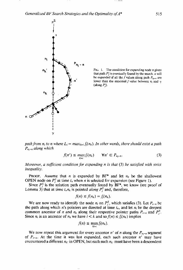
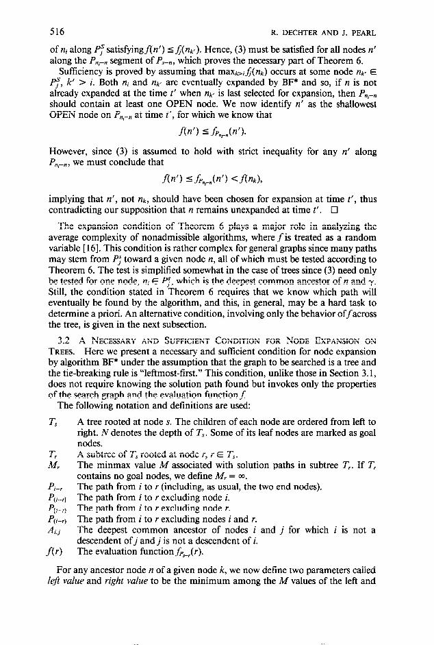
THEOREM 6. Let Pi” be the solution path eventually found by BE* and let ni be the depth-i node along PJ, i = 0, 1, . . . . A necessary condition for expanding an arbitrary node n in the graph is that, for some nj E Pi”, there exists an Li-bounded
Generalized BF Search Strategies and the Optimality ofA* 515
P lli - n
n’
FIG. 1, The condition for expanding node n given that path Pj is eventually found by the search. n will be expanded if all the f values along path P,,,-, are lower than the maximal f value between ni and y (along PJ).
Y
path from ni to n where Li = maxbiJ(nk). In other words, there should exist a path P,,,-, along which
.fW) 5 mE,d(nk) Vn’ E P,,-,. (3)
Moreover, a suficient condition for expanding n is that (3) be satisfied with strict inequality.
PROOF. Assume that n is expanded by BF* and let & be the shallowest OPEN node on Pf at time tn when n is selected for expansion (see Figure 1).
Since PT is the solution path eventually found by BF*, we know (see proof of Lemma 3) that at time tnnk is pointed along Py and, therefore,
f(n) 5 f(nk) = A@k>-
We are now ready to identify the node ni on Ps, which satisfies (3). Let PST,, be the path along which n’s pointers are directed at time t,,, and let ni be the deepest common ancestor of n and nk along their respective pointer paths PS-, and PT. Since ni is an ancestor of nk we have i < k and so f(n) 5 A:<&) implies
We now repeat this argument for every ancestor n’ of n along the P,,-, segment of PS-,. At the time it was last expanded, each such ancestor n’ may have encountered a different nk’ in OPEN, but each such rzk must have been a descendent
516 R. DECHTER AND J. PEARL
of ni along PT satisfyingf(n’) 5 A(np). Hence, (3) must be satisfied for all nodes n’ along the P,,,-, segment of P,-,, which proves the necessary part of Theorem 6.
Sufficiency is proved by assuming that maxb&nk) occurs at some node nk’ E Pi”, k’ > i. Both ni and nk’ are eventually expanded by BF* and so, if n is not already expanded at the time t’ when ne is last selected for expansion, then P,,,-, should contain at least one OPEN node. We now identify n’ as the shallowest OPEN node on P,,-, at time t’, for which we know that
f(n’) = fP,,,W).
However, since (3) is assumed to hold with strict inequality for any n’ along P,,i-,, we must conclude that
f(n’> 5 fp,,,(n’) < f(nkh
implying that n’, not nk, should have been chosen for expansion at time t’, thus contradicting our supposition that n remains unexpanded at time t’. 0
The expansion condition of Theorem 6 plays a major role in analyzing the average complexity of nonadmissible algorithms, where f is treated as a random variable [ 161. This condition is rather complex for general graphs since many paths may stem from PJ toward a given node n, all of which must be tested according to Theorem 6. The test is simplified somewhat in the case of trees since (3) need only be tested for one node, ni E Pj”, which is the deepest common ancestor of n and y. Still, the condition stated in Theorem 6 requires that we know which path will eventually be found by the algorithm, and this, in general, may be a hard task to determine a priori. An alternative condition, involving only the behavior offacross the tree, is given in the next subsection.
3.2 A NECESSARY AND SUFFICIENT CONDITION FOR NODE EXPANSION ON TREES. Here we present a necessary and sufficient condition for node expansion by algorithm BF* under the assumption that the graph to be searched is a tree and the tie-breaking rule is “leftmost-first.” This condition, unlike those in Section 3.1, does not require knowing the solution path found but invokes only the properties of the search graph and the evaluation functionf:
The following notation and definitions are used:
T,
T, M,
Pi-r
fli-r]
P[i-r)
P(i-r)
-4.j
f(r)
A tree rooted at node s. The children of each node are ordered from left to right. N denotes the depth of T,. Some of its leaf nodes are marked as goal nodes. A subtree of T, rooted at node r, r E T,. The minmax value A4 associated with solution paths in subtree T,. If T, contains no goal nodes, we define M, = 00. The path from i to r (including, as usual, the two end nodes). The path from i to r excluding node i. The path from i to r excluding node r. The path from i to r excluding nodes i and r. The deepest common ancestor of nodes i and j for which i is not a descendent ofj and j is not a descendent of i. The evaluation function fps,( r).
For any ancestor node n of a given node k, we now define two parameters called lefi value and right value to be the minimum among the M values of the left and
Generalized BF Search Strategies and the Optimality ofA* 5
517
k . . .
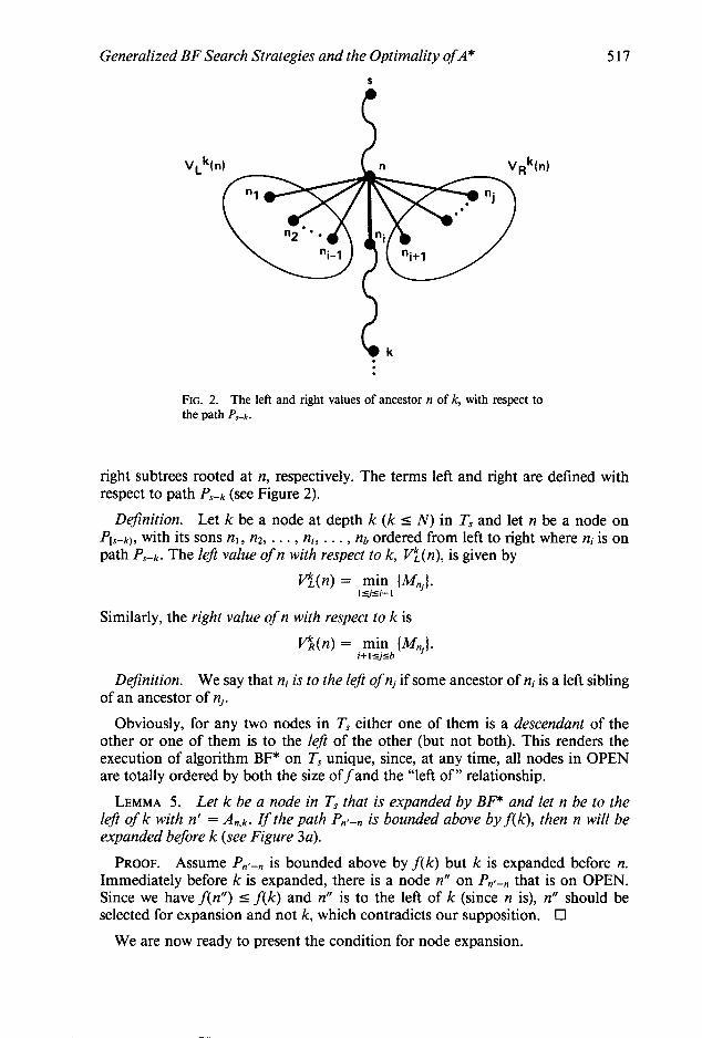
FIG. 2. The left and right values of ancestor n of k, with respect to the path Prk.
right subtrees rooted at n, respectively. The terms left and right are defined with respect to path Ps-k (See Figure 2).
Definition. Let k be a node at depth k (k I N) in T, and let n be a node on Pts+, with its sons nl, n2, . . . , ni, . . . , nb ordered from left to right where ni is on path P&. The left value of n with respect to k, V:(n), is given by
V:(n) = mm V&,1. I sjsi- I
Similarly, the right value of n with respect to k is
Vi(n) = min (Mnjl. i+lsjjsb
Definition. We say that ni is to the left of nj if some ancestor of ni is a left sibling of an ancestor of nj.
Obviously, for any two nodes in T, either one of them is a descendant of the other or one of them is to the left of the other (but not both). This renders the execution of algorithm BF* on T, unique, since, at any time, all nodes in OPEN are totally ordered by both the size off and the “left of” relationship.
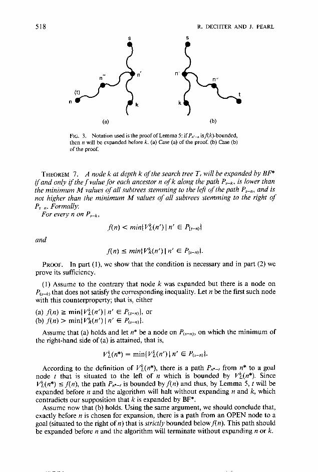
LEMMA 5. Let k be a node in T, that is expanded by BFC and let n be to the left of k with n’ = A,,,k. If the path P,,,-, is bounded above by f(k), then n will be expanded before k (see Figure 3a).
PROOF. Assume P,,-, is bounded above by f(k) but k is expanded before n. Immediately before k is expanded, there is a node n” on P,,-, that is on OPEN. Since we have f(n”) 5 f(k) and n” is to the left of k (since n is), n” should be selected for expansion and not k, which contradicts our supposition. Cl
We are now ready to present the condition for node expansion.
518
S
R. DECHTER AND J. PEARL
n
--4* n”
(t)
n k
n’
k
FIG. 3. Notation used is the proof of Lemma 5; if I’,.-,, isf(k)-bounded, then n will be expanded before k. (a) Case (a) of the proof. (b) Case (b) of the proof.
THEOREM 7. A node k at depth k of the search tree T, will be expanded by BE* if and only tf the f value for each ancestor n of k along the path Ps+ is lower than the minimum A4 values of all subtrees stemming to the left of the path P,-.,, and is not higher than the minimum M values of all subtrees stemming to the right of P,-, . Formally:
For every n on Ps-k,
f(n) < min{Vi(n’) ) n’ E P(S-njl
and f(n) 5 min( Vi(n’) 1 n’ E PI,-,,].
PROOF. In part (1) we show that the condition is necessary and in part (2) we prove its sufficiency.
(1) Assume to the contrary that node k was expanded but there is a node on PCs+) that does not satisfy the corresponding inequality. Let n be the first such node with this counterproperty; that is, either
(a) f(n) 2 min(Vi(n’) 1 n’ E PcS+j), or (b) f(n) > min( Vi(n’) 1 n’ E PcS-,,).
Assume that (a) holds and let n* be a node on PC,-,), on which the minimum of the right-hand side of (a) is attained, that is,
Vi(n*) = min( Vi(n’) I n’ E Pc~-~,].
According to the definition of V!L(n*), there is a path P,,v from n* to a goal node t that is situated to the left of n which is bounded by Vi(n*). Since Vi(n*) 5 f(n), the path P,,L~ is bounded by f(n) and thus, by Lemma 5, t will be expanded before n and the algorithm will halt without expanding n and k, which contradicts our supposition that k is expanded by BF*.
Assume now that (b) holds. Using the same argument, we should conclude that, exactly before n is chosen for expansion, there is a path from an OPEN node to a goal (situated to the right of n) that is strictly bounded below f(n). This path should be expanded before n and the algorithm will terminate without expanding n or k.
Generalized BF Search Strategies and the Optimality ofA* 519
(2) Let k be a node at depth k that satisfies the condition. We show that k must be expanded by BF*. Let t be the goal node on which BF* halts. If t is a descendant of k, then, obviously, k must be expanded. Otherwise, t is either to the left of k or to its right.
Case 1. t is to the left of k. Let n’ = At,k, n’ is on the path Ps-k. Let M be the maxfvalue on Pcn,-l~ and n” E Pcn,-t~ with f(n”) = M (see Figure 3a). Since t is expanded, n’ must be expanded, and, therefore, before the algorithm expands n”, there is always an OPEN node on PC,,,+. From the condition of the theorem,
f(n) < M = f(n”) Vn E Pw-kl, and therefore all the nodes on Pen,+] must be expanded before n”. Knowing that n” is expanded implies the expansion of k and all its ancestors.
Case 2. t is to the right of k. The situation in this case is shown in Figure 3b. From the condition of the theorem, it follows that the path Pen,+ is bounded below f(n”) and therefore, from Lemma 5, k should be expanded before n”. Cl
4. On the Optimality of A* 4.1 PREVIOUS WORKS AND THE NOTION OF EQUALLY INFORMED ALGO-
RITHMS. The optimality of A*, in the sense of computational eficiency, has been a subject of some confusion. The well-known property of A*, which predicts that decreasing errors h * - h can only improve its performance [ 14, result 61, has often been interpreted to reflect some supremacy of A* over other search algorithms of equal information. Consequently, several authors have assumed that optimality of A* is an established fact (e.g., [2, 12, 131). In fact, all this property says is that some A* algorithms are better than other A* algorithms, depending on the heuristics that guide them. It does not indicate whether the additive rulef= g + h is the best way of combining g and h; neither does it assure us that expansion policies based only on g and h can do as well as more sophisticated policies that use the entire information gathered by the search. These two conjectures are examined in this section, and are given a qualified confirmation.
The first attempt to prove the optimality of A* was carried out by Hart et al. [6, 71 and is summarized in Nilsson [ 131. Basically, Hart et al. argue that if some admissible algorithm B fails to expand a node n expanded by A*, then B must have known that any path to a goal constrained to go through node n is nonoptimal. A*, by comparison, had no way of realizing this fact because when n was chosen for expansion it satisfied g(n) + h(n) 5 C*, clearly advertising its promise to deliver an optimal solution path. Thus, the argument goes, B must have obtained extra information from some external source, unavailable to A* (perhaps by computing a higher value for h(n)), and this disqualifies B from being an “equally informed,” fair competitor to A*.
The weakness of this argument is that it fails to account for two legitimate ways in which B can decide to refrain from expanding n based on information perfectly accessible to A*. First, B may examine the properties of previously exposed portions of the graph and infer that n actually deserves a much higher estimate than h(n). On the other hand, A*, although it has the same information available to it in CLOSED, cannot put it into use because it is restricted to take the estimate h(n) at face value and only judge nodes by the score g(n) + h(n). Second, B may also gather information while exploring sections of the graph unvisited by A*, and this should not render. B an unfair, “more informed” competitor to A* because, in
520 R. DECHTER AND J. PEARL
principle, A* too had an opportunity to visit those sections of the graph. Later in this section (see Figure 6), we demonstrate the existence of an algorithm B, which manages to outperform A* using this kind of information.
Gelperin [4] has correctly pointed out that, in any discussion of the optimality of A*, one should also consider algorithms that adjust their h in accordance with the information gathered during the search. His analysis, unfortunately, falls short of considering the entirety of this extended class, having to follow an overrestrictive definition of equally informed. Gelperin’s interpretation of “an algorithm B [that] is never more informed than A*,” instead ofjust restricting B from using information inaccessible to A, actually forbids B from processing common information in a better way than A does. For example, if B is a best-first algorithm guided by fB, then in order to qualify for Gelperin’s definition of “never more informed than A*,” B is forbidden from ever assigning to a node y1 a value &(n) higher than g(n) + h(n), even if the information gathered along the path to n justifies such an assignment.
In our analysis, we use the natural definition of “equally informed,” allowing the algorithms compared to have access to the same heuristic information while placing no restriction on the way they use it. Accordingly, we assume that an arbitrary heuristic function h(n) is assigned to the nodes of G and that the value h(n) is made available to each algorithm that chooses to generate node n. This amounts to viewing h(n) as part of the parameters that specify problem instances, and, correspondingly, we represent each problem instance by the quadruple I = (G, s, r, h).
We demand, however, that A* only be compared to algorithms that return optimal solutions in those problem instances where their computational perform- ances are to be appraised. In particular, if our problem space contains only cases in which h(n) 5 h*(n) for every 12 in G, we only consider algorithms that, like A*, return least-cost solutions in such cases. The class of algorithms answering this conditional admissibility requirement is simply called admissible and is denoted by Aad. From this general class of algorithms, we later examine two subclasses A, and Abf. A, denotes the class of algorithms that are globally compatible with A*, that is, they return optimal solutions whenever A* does, even in cases where h > h*. Abr stands for the class of admissible BF* algorithms, that is, those that conduct their search in a best-first manner, being guided by a path-dependent evaluation function as in Section 1.
Additionally, we assume that each algorithm compared with A* uses the primitive computational step of node expansion, that it only expands nodes that were generated before, and that it begins the expansion process at the start node s. This excludes, for instance, bidirectional searches [ 191 or algorithms that simultaneously grow search trees from several “seed nodes” across G.
4.2. NOMENCLATURE AND A HIERARCHY OF OPTIMALITY RELATIONS. Our notion of optimality is based on the usual requirement of dominance [ 141.
Definition. Algorithm A is said to dominate algorithm B relative to a set I of problem instances iff in every instance I E I, the set of nodes expanded by A is a subset of the set of nodes expanded by B. A strictly dominates B iff A dominates B and B does not dominate A, that is, there is at least one instance when A skips a node that B expands, and no instance when the opposite occurs.
This definition is rather stringent because it requires that A establish its supe- riority over B under two difficult tests:
Generalized BF Search Strategies and the Optimality ofA* 521
(1) expanding a subset of nodes rather than a smaller number of nodes, (2) outperforming B in every problem instance rather than in the majority of
instances.
Unfortunately, there is no easy way of loosening any of these requirements without invoking statistical assumptions regarding the relative likelihood of instances in I. In the absence of an adequate statistical model, requiring dominance remains the only practical way of guaranteeing that A expandsfewer nodes than B, because, if in some problem instance we were to allow B to skip even one node that is expanded by A, one could immediately present an inlinite set of instances when B grossly outperforms A. (This is normally done by appending to the node skipped a variety of trees with negligible costs and very low h.)
Adhering to the concept of dominance, the strong definition of optimality proclaims algorithm A optimal over a class A of algorithms iff A dominates every member of A. Here the combined multiplicity of A and I also permits weaker definitions; for example, we may proclaim A weakly optimal over A if no member of A strictly dominates A. The spectrum of optimality conditions becomes even richer when we examine A*, which stands for not just one but a whole family of algorithms, each defined by the tie-breaking rule chosen. We chose to classify this spectrum into the following four types (in a hierarchy of decreasing strength):
Type 0. A* is said to be O-optimal over A relative to I iff, in every problem instance, Z E I, every tie-breaking rule in A* expands a subset of the nodes expanded by any member of A. (In other words, every tie-breaking rule dominates all members of A.)
Type 1. A* is said to be l-optimal over A relative to I iff, in every problem instance, Z E I, there exists at least one tie-breaking rule that expands a subset of the set of nodes expanded by any member of A.
Type 2. A* is said to be 2-optimal over A relative to I iff there exists no problem instance Z E I in which some member of A expands a proper subset of the set of nodes that are expanded by some tie-breaking rule in A*.
Type 3. A* is said to be 3-optimal over A relative to I iff the following holds: If there exists a problem instance Ii E I where some algorithm B E A skips a node expanded by some tie-breaking rule in A*, then there must also exist some problem instance Z2 E I where that tie-breaking rule skips a node expanded by B. (In other words, no tie-breaking rule in A* is strictly dominated by some member of A.)
Type 1 describes the notion of optimality most commonly used in the literature, and it is sometimes called “optimal up to a choice of a tie-breaking rule.” Note that these four definitions are applicable to any class of algorithms, B, contending to be optimal over A; we need only replace the words “tie-breaking rule in A*” by the words “member of B.” If B turns out to be a singleton, then type 0 and type 1 collapse to strong optimality. Type 3 will collapse into type 2 if we insist that I, be identical to Z2.
We are now ready to introduce the four domains of problem instances over which the optimality of A* is to be examined. The first two relate to the admissibility and consistency of h(n).
Definition. A heuristic function h(n) is said to be admissible on (G, I’) iff h(n) I h*(n) for every n E G.

522 R. DECHTER AND J. PEARL
Deftnition. A heuristic function h(n) is said to be consistent (or monotone) on G iff, for any pair of nodes ~1’ and n, the triangle inequality holds:
h(n’) 5 k(n’, n) + h(n).
Corresponding to these two properties, we define the following sets of problem instances:
IAD = ((G, s, F, h) 1 h 5 h* on (G, I’)), ICON = ((G, s, I’, h) 1 h is consistent on G) .
Clearly, consistency implies admissibility [ 161 but not vice versa; therefore, ICON G IAD.
A special and important subset of I AD (and IcoN), called nonpathological in- stances, are those instances for which there exists at least one optimal solution path along which h is not fully informed; that is, h < h* for every nongoal node on that path. The nonpathological subsets of I AD and IcoN are denoted by I~D and I.&+ respectively.
It is known that, if h 5 h*, then A* expands every node reachable from s by a strictly C*-bounded path, regardless of the tie-breaking rule used. The set of nodes with this property is referred to as surely expanded by A*. In general, for an arbitrary constant d and an arbitrary evaluation function fover (G, s, I’, h), we let NJ” denote the set of all nodes reachable from s by some strictly d-bounded path in G. For example, NgJh is a set of nodes surely expanded by A* in some instance of I AD.
The importance of nonpathological instances lies in the fact that in such instances the set of nodes surely expanded by A* are indeed all the nodes expanded by it. Therefore, for these instances, any claim regarding the set of nodes surely expanded by A* can be translated to “the set of all the nodes” expanded by A*. This is not the case, however, for pathological instances in I AD; N$:h is often a proper subset of the set of nodes actually expanded by A*. If h is consistent, then the two sets differ only by nodes for which h(n) = C* - g*(n) [ 161. However, in cases in which h is inconsistent, the difference may be very substantial; each node n for which h(n) = C* - g*(n) may have many descendents assigned lower h values (satisfying h + g < C*) and these descendants may be expanded by every tie-breaking rule of A* even though they do not belong to Ng$.
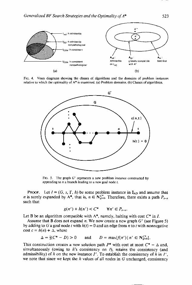
In Section 4.3 we present several theorems regarding the behavior of competing classes of algorithms relative to the set NgTh of nodes surely expanded by A*, and we interpret these theorems as claims about the type of optimality that A* enjoys over the competing classes. Moreover, for any given pair (A, I) where A is a class of algorithms drawn from (Aad, AM, Age) and I is a domain of problem instances from {IAD, IAD, ICON, I&J, we determine the strongest type of optimality that can be established over A relative to I and identify the algorithm that achieves this optimality. The relationships between these classes of algorithms and problem domains are shown in Figure 4. The algorithm A** is an improvement over A* discussed in Appendix B.
4.3 WHERE AND HowIsA* OPTIMAL?
4.3.1 Optimality over Admissible Algorithms, A,d
THEOREM 8. Any algorithm that is admissible on IAD will expand, in every instance I E ICON, all nodes surely expanded by A*.
Generalized BF Search Strategies and the Optimality ofA* 523
IAD: h admissible
IiD: h admissible nonpathological
IcoN: h consistent
Aad Age : 41 :
I&,,,: h consistent nonpathological
admissible
on ‘AD
globally compatible with A’
best-first
(4 (b) FIG. 4. Venn diagrams showing the classes of algorithms and the domains of problem instances relative to which the optimality of A* is examined. (a) Problem domains. (b) Classes of algorithms.
G’
FIG. 5. The graph G’ represents a new problem instance constructed by appending to n a branch leading to a new goal node t.
PROOF. Let Z = (G, S, I’, h) be some problem instance in IAn and assume that n is surely expanded by A*, that is, n E Ng$,. Therefore, there exists a path P,-, such that
g(n’) + h(n’) < C* Vn’ E P,-,.
Let B be an algorithm compatible with A*, namely, halting with cost C* in I. Assume that B does not expand n. We now create a new graph G’ (see Figure 5)
by adding to G a goal node t with h(t) = 0 and an edge from n to t with nonnegative cost c = h(n) + A, where
A = ;(C* - D) > 0 and D = max(f(n’) 1 n’ E N$h].
This construction creates a new solution path P* with cost at most C* - A and, simultaneously (owing to h’s consistency on I), retains the consistency (and admissibility) of h on the new instance I’. To establish the consistency of h in I’, we note that since we kept the h values of all nodes in G unchanged, consistency
524 R. DECHTER AND J. PEARL
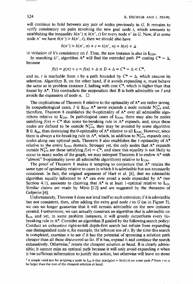
will continue to hold between any pair of nodes previously in G. It remains to verify consistency on pairs involving the new goal node t, which amounts to establishing the inequality h(n’) I k(n’, t) for every node n’ in G. Now, if at some node 0 we have h(n’) > k(n’, t), then we should also have
h(d) > k(n’, n) + c = k(n’, n) + h(n) + A
in violation of h’s consistency on I. Thus, the new instance is also in ICON. In searching G’, algorithm A* will find the extended path P* costing C* - A,
because
fit) = g(n) -t c =f(n) + A 5 D -t A = C* - A < C*,
and so, t is reachable from s by a path bounded by C* - A, which ensures its selection. Algorithm B, on the other hand, if it avoids expanding n, must behave the same as in problem instance Z, halting with cost C*, which is higher than that found by A*. This contradicts the supposition that B is both admissible on Z and avoids the expansion of node n. Cl
The implications of Theorem 8 relative to the optimality of A* are rather strong. In nonpathological cases, Z E I- cog A* never expands a node outside N$:h and, therefore, Theorem 8 establishes the 0-optimality of A* over all admissible algo- rithms relative to I&+ In pathological cases of ICON, there may also be nodes satisfying f(n) = C* that some tie-breaking rule in A* expands, and, since these nodes are defined to be outside N$,, they may be avoided by some algorithm B E Aad, thus destroying the 0-optimality of A* relative to all ICON. However, since there is always a tie-breaking rule in A*, which, in addition to Ns:h, expands only nodes along one optimal path, Theorem 8 also establishes the 1-optimality of A* relative to the entire IcoN domain. Stronger yet, the only nodes that A* expands outside NzJh are those satisfyingf(n) = C*, and since this equality is not likely to occur in many nodes of the graph, we may interpret Theorem 8 to endow A* with “almost” 0-optimality (over all admissible algorithms) relative to IcoN.
The proof of Theorem 8 makes it tempting to conjecture that A* retains the same type of optimality relative to cases in which h is admissible but not necessarily consistent. In fact, the original argument of Hart et al. [6], that no admissible algorithm equally informed to A* can ever avoid a node expanded by A* (see Section 4.1), amounts to claiming that A* is at least l-optimal relative to IAn. Similar claims are made by Miro [ 121 and are suggested by the theorems of Gelperin [4].
Unfortunately, Theorem 8 does not lend itself to such extension; if h is admissible but not consistent, then, after adding the extra goal node t to G (as in Figure 5), we can no longer guarantee that h will remain admissible on the new instance created. Furthermore, we can actually construct an algorithm that is admissible on IAD, and yet, in some problem instances, it will grossly outperform every tie- breaking rule in A*. Consider an algorithm B guided by the following search policy: Conduct an exhaustive right-to-left depth-first search but refrain from expanding one distinguished node 12, for example, the leftmost son of s. By the time this search is completed, examine n to see if it has the potential of sprouting a solution path cheaper than all those discovered so far. If it has, expand it and continue the search exhaustively. Otherwise,3 return the cheapest solution at hand. B is clearly admis- sible; it cannot miss an optimal path because it will only avoid expanding n when it has sufficient information to justify this action, but otherwise will leave no stone 3 A simple valid test for skipping a node in I A~ is that max(g(n) + h(n) 1 n) on some path P from s to n be larger than the cost of the cheapest solution at hand.

Generalized BF Search Strategies and the Optimality ofA* 525
(4
JI
h=l
J2
. .
. .
. .
(b)
FIG. 6. Graphs demonstrating that A* is not optimal. (a) A nonpathological problem where algorithm B will avoid a node (JI) that A* must expand. (b) A pathological graph (f(J2) = Cc = II) where algorithm B expands a proper subset of the nodes expanded by A*.
unturned. Yet, in the graph of Figure 6a, B will avoid expanding many nodes that are surely expanded by A*. A* will expand node Jr immediately after s because (f(J1) = 4) and subsequently will also expand many nodes in the subtree rooted at J,. B, on the other hand, will expand J3, then select for expansion the goal node y, continue to expand Jz, and, at this point, halt without expanding node J1. Relying on the admissibility of h, B can infer that the estimate h(J,) = 1 is overly optimistic and should be at least equal to h(J2) - 1 = 19, thus precluding J1 from lying on a solution path cheaper than the path (s, I, y) at hand.
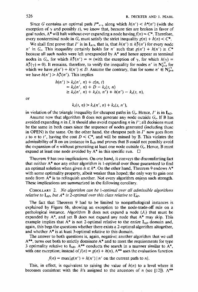
Granted that A* is not l-optimal over all admissible algorithms relative to IAD, the question arises if a l-optimal algorithm exists altogether. Clearly, if a l-optimal algorithm exists, it would have to be better than A* in the sense of skipping, in some problem instances, at least one node surely expanded by A*, while never expanding a node that is surely skipped by A*. Note that algorithm B could not be such an optimal algorithm because, in return for skipping node JI in Figure 6a, it had to pay the price of expanding Jz, and Jz will not be expanded by A* regardless of the tie breaking rule invoked. If we could show that this “node trade-off pattern must hold for every admissible algorithm and on every instance of IAD, then we would have to conclude both that no l-optimal algorithm exists and that A* is 2- optimal relative to this domain. Theorem 9 accomplishes this task relative to IAn.
THEOREM 9. If an admissible algorithm B does not expand a node that is surely expanded by A* in some problem instance when h is admissible and nonpatholog- ical, then, in that very problem instance, B must expand a node that is avoided by every tie-breaking rule in A*.
PROOF. Assume the contrary, that is, that there is an instance I = (G, s, P, h) E Iin such that a node n that is surely expanded by A* is avoided by B and, at the same time, B expands no node that is avoided by A*. We show that this assumption implies the existence of another instance I’ E IAD for which B will not find an optimal solution. I’ is constructed by taking the graph G, exposed by the run of A* (including nodes in OPEN) and appending to it another edge (n, t) to a new goal node t, with cost c(n, t) = D - ke(s, n) where
D = maxlf(n’) 1 n’ E N$],
and ke(n’, n) is the cost of the cheapest path from n’ to n in G,.
526 R. DECHTER AND J. PEARL
Since G contains an optimal path P*,-, along which h(n’) < h*(n’) (with the exception of y and possibly s), we know that, because ties are broken in favor of goal nodes, A* will halt without ever expanding a node havingf( n) = C*. Therefore, every nonterminal node in G, must satisfy the strict inequality g(n) + h(n) < C*.
We shall first prove that I’ is in I *n, that is, that h(n’) I h?(n’) for every node ~1’ in G,. This inequality certainly holds for n’ such that g(n’) + h(n’) I C* because all such nodes were left unexpanded by A* and hence appear as terminal nodes in G,, for which h?(n’) = 03 (with the exception of y, for which h(r) = h?(r) = 0). It remains, therefore, to verify the inequality for nodes n’ in N,J:h for which we have g(n’) + h(n’) 5 D. Assume the contrary, that for some n’ E NgJh we have h(n’) > h:(n’). This implies
h(n’) > k,(n’, n) + c(n, t) = k,(n’, n) + D - ke(s, n) 5 k,(n’, n) + k,(s, n’) + h(n’) - ke(s, n),
or
Us, n) > Un’, n) + k&, ~1’1,
in violation of the triangle inequality for cheapest paths in G,. Hence, I’ is in IAD. Assume now that algorithm B does not generate any node outside G,. If B has
avoided expanding n in 1, it should also avoid expanding n in I’; all decisions must be the same in both cases since the sequence of nodes generated (including those in OPEN) is the same. On the other hand, the cheapest path in I’ now goes from s to n to t’, having the cost D < C*, and will be missed by B. This violates the admissibility of B on an instance in I AD and proves that B could not possibly avoid the expansion of n without generating at least one node outside G,. Hence, B must expand at least one node avoided by A* in this specific run. Cl
Theorem 9 has two implications. On one hand, it conveys the discomforting fact that neither A* nor any other algorithm is l-optimal over those guaranteed to find an optimal solution when given h I h*. On the other hand, Theorem 9 endows A* with some optimality property, albeit weaker than hoped; the only way to gain one node from A* is to relinquish another. Not every algorithm enjoys such strength. These implications are summarized in the following corollary.
COROLLARY 2. No algorithm can be I-optimal over all admissible algorithms relative to IAD, but A* is 2-optimal over this class relative to I;;o.
The fact that Theorem 9 had to be limited to nonpathological instances is explained by Figure 6b, showing an exception to the node-trade-off rule on a pathological instance. Algorithm B does not expand a node (JJ that must be expanded by A*, and yet B does not expand any node that A* may skip. This example implies that A* is not 2-optimal relative to the entire IAD domain and, again, this begs the questions whether there exists a 2-optimal algorithm altogether, and whether A* is at least 3-optimal relative to this domain.
The answer to both questions is, again, negative; another algorithm that we call A**, turns out both to strictly dominate A* and to meet the requirements for type 3 optimality relative to IAD. A** conducts the search in a manner similar to A*, with one exception; instead off(n) = g(n) + h(n), A** uses the evaluation function
f(n) = max(g(n’) + h(n’) 1 n’ on the current path to n).
This, in effect, is equivalent to raising the value of h(n) to a level where it becomes consistent with the h’s assigned to the ancestors of n (see [ 121). A**
Generalized BF Search Strategies and the Optimality ofA* 527
chooses for expansion the nodes with the lowest f value in OPEN (breaking ties arbitrarily, but in favor of goal nodes) and adjusts pointers along the path having the lowest g value. In Figure 6a, for example, if A** ever expands node Jz, then its son J, will immediately be assigned the value f( J,) = 2 1 and its pointer directed toward J2.
It is possible to show (see Appendix B) that A** is admissible and that in nonpathological cases A** expands the same set of nodes as does A*, namely, the surely expanded nodes in Ng;h. In pathological cases, however, there exist tie- breaking rules in A** that strictly dominate every tie-breaking rule in A*. This immediately precludes A* from being 3-optimal relative to IAD and nominates A** for that title.
THEOREM 10. Let a** be some tie-breaking rule in A** and B an arbitrary algorithm, admissible relative to I AD. If in some problem instance I, E IAD, B skips a node expanded by a ** then there exists another instance I2 E IAD where B , expands a node skipped by a**.
PROOF. Let
SA = nl, n2, . . . , nk, J, . . . and
SB = nl, n2, . . . , nk, K, . . .
be the sequences of nodes expanded by a** and B, respectively, in problem instance 1, E IAb, that is, K is the first node in which the sequence S, deviates from S,. Consider G,, the explored portion of the graph just before a** expands node J. That same graph is also exposed by B before it decides to expand K instead. Now construct a new problem instance 12 consisting of G, appended by a branch (J, t) with cost c(J, t) = f(J) - g(J), where t is a goal node and f(J) and g(J) are the values that a** computed for J before its expansion. 12 is also in LD because h(t) = 0 and c( J, t) are consistent with h(J) and with the h’s of all ancestors of J in G,. For, if some ancestor ni of J satisfies h( ni) > h*( ni), we obtain a contradiction
g(nJ + h(nd > g(nJ + h*(nJ = g(nJ + Uni, 4 + 4J, t) = g(J) + 4J, t) = f(J) G max[g(nj) + h(nj)].
i Moreover, a** will expand in 12 the same sequence of nodes as it did in I,,
until J is expanded, at which time t enters OPEN with f(t) = max[g(J) + c(J, t), f( J)l = f( J). N ow, since J was chosen for expansion by virtue of its lowest f value in OPEN, and since a** always breaks up ties in favor of a goal node, the next and final node that a** expands must be t. Now consider B. The sequence of nodes it expands in I2 is identical to that traced in II because, by avoiding node J, B has no way of knowing that a goal node has been appended to G,. Thus, B will expand K (and perhaps more nodes on OPEN), a node skipped by a**. Cl
Note that the special evaluation function used by A** f(n) = max(g(n’) + h(n ‘) 1 n’ on P,_,) was necessary to ensure that the new instance, 12, remains in IAD. The proof cannot be carried out for A* because the evaluation function f(n) = g(n) + h(n) results in c(J, t) = h(J), which may lead to violation of h(ni) 5 h*(ni) for some ancestor of J.
Theorem 10, together with the fact that its proof makes no use of the assumption that B is admissible, gives rise to the following conclusion.
528 R. DECHTER AND J. PEARL
COROLLARY 3. A** is 3-optimal over all algorithms relative to IAD.
Theorem 10 also implies that there is no 2-optimal algorithm over Aad relative to IAn. From the 3-optimality of A** we conclude that every 2-optimal algorithm, if such exists, must be a member of the A** family, but Figure 6b demonstates an instance of IAD where another algorithm (B) only expands a proper subset of the nodes expanded by every member of A . ** This establishes the following desired conclusion.
COROLLARY 4. There is no 2-optimal algorithm over Aad relative to IAD.
4.3.2 Optimality over Globally Compatible Algorithms, Age So far, our anal- ysis was restricted to algorithms in Aad, that is, those that return optimal solutions if h(n) I h*(n) for all n, but that may return arbitrarily poor solutions if there are some n for which h(n) > h*(n). In situations in which the solution costs are crucial and in which h may occasionally overestimate h*, it is important to limit the choice of algorithms to those which return reasonably good solutions even when h > h*. A*, for example, provides such guarantees; the costs of the solutions returned by A* do not exceed C* + A where A is the highest error h*(n) - h(n) over all nodes in the graph [5], and, moreover, A* still returns optimal solutions in many problem instances, that is, whenever A is zero along some optimal path. This motivates the definition of A,, the class of algorithms globally compatible with A*; namely, they return optimal solutions in every problem instance in which A* returns such solution.
Since A, is a subset of Aad, we should expect A* to hold a stronger optimality status over A,, at least relative to instances drawn from IAn. The following theorem confirms this expectation.
THEOREM 11. In problem instances in which h is admissible, any algorithm that is globally compatible with A* will expand all nodes surely expanded by A*.
PROOF. Let I = (G, s, T, h) be some problem instance in IAD and let node n be surely expanded by A*; that is, there exists a path PS-, such that
g(n) + h(n) c C* Vn’ E P,-,.
Let D = max(f(n’) ] n’ E P,_,,) and assume that some algorithm B E A, fails to expand n. Since I E IAD, both A* and B will return cost C*, while D < C*.
We now create a new graph G’, as in Figure 5, by adding to G a goal node t’ with h(t’) = 0 and an edge from n to t’ with nonnegative cost D - g(PS-,). Denote the extended path PS-,-lf by P*, and let I’ = (G’, s, l? U t’, h) be a new instance in the algorithms’ domain. Although h may no longer be admissible on I’, the construction of I’ guarantees thatf(n’) 5 D if n’ E P*, and thus, by Theorem 2, algorithm A* searching G’ will find an optimal solution path with cost Cl 5 M 5 D. Algorithm B, however, will search I’ in exactly the same way it searched I; the only way B can reveal any difference between I and I’ is by expanding n. Since it did not, it will not find solution path P*, but will halt with cost C* > D, the same cost it found for I and worse than that found by A*. This contradicts its property of being globally compatible with A*. 0
COROLLARY 5. A* is O-optimal over Age relative to IAD.
The corollary follows from the fact that in nonpathological instances A* expands only surely expanded nodes.
Generalized BF Search Strategies and the Optimality ofA* 529
COROLLARY 6. A* is l-optimal over Age relative to IAD.
PROOF. The proof relies on the observation that, for every optimal path P* (in any instance of IX,), there is a tie-breaking rule of A* that expands only nodes along P* plus perhaps some other nodes having g(rz) + h(n) c C*; that is, the only nodes expanded satisfying the equality g(n) + h(n) = C* are those on P*. Now, if A* is not l-optimal over A,, then, given an instance Z, there exists an algorithm B E A,, such that B avoids some node expanded by all tie-breaking rules in A*. To contradict this supposition, let A: be the tie-breaking rule of A* that returns the same optimal path P* as B returns, but expands no node outside P* for which g(n) + h(n) = C*. Clearly, any node n that B avoids and AT expands must satisfy g(n) -I- h(n) < C*. We can now apply the argument used in the proof of Theorem 11, appending to n a branch to a goal node t’, with cost c(n, t’) = h(n). Clearly, A? will find the optimal path (s, n, t’) costing g(n) + h(n) < C*, whereas B will find the old path costing C*, thus violating its global compatibility with A*. Cl
4.3.3 Optimality over Best-First Algorithms, Abf. The next result establishes the optimality of A* over the set of best-first algorithms (BF*), which are admissible if provided with h 5 h*. These algorithms are permitted to employ any evaluation function fP, where f is a function of the nodes, the edge-costs, and the heuristic function h evaluated on the nodes of P, that is,
fp Af(s, nl, 122, . . . , n) =f(lni), (c(ni, ni+Ol, ih(ni)I I ni E 0.
LEMMA 6. Let B be a BF* algorithm using an evaluation function fe such that for every (G, s, r, h) E IAD fe satisfies
fp: = f(s, nl, n2, . . . , -r) = C(E) tly E r.
If B is admissible on IAD, then N$h c NT.
PROOF. Let I = (G, s, r, h) E IAD and assume n E NF!h but n 4 Nx; that is, there exists a path P,-, such that for every n’ E P,-, gp(n’) + h(n’) < C* and, for some n’ E P,-,, fB(n’) 2 C*.
Let
QB =,EF-, (fB( n ’ ) ) .
Obviously, Q < C* and QB 2 C* + QB > Q. Define G’ to include path Ps-, with two additional goal nodes tl, t2 as described by Figure 7. The cost on edge (s, t2) is ( QB + Q)/2; the cost on edge (n, tl) is Q - gp,,(n); tl and t2 are assigned h ’ = 0, while all other nodes retain their old h. I’ = (G’, s, r U (tl, t2), h) E IAn since Vn’, n’ E P,-,, g(n’) + h(n’) 5 Q, which implies that h(n’) 5 Q - g(n’) = h?(n’).
Obviously the optimal path in G’ is P,-.I, with cost Q. However, following the condition of the lemma, the evaluation function fB satisfies
MP+~, =Mtd = C(Ps-t,) = v < QB.
Moreover, since MpS-,, 2 QB, we have Mp,-,, < MpS-, , implying that B halts on the suboptimal path P,-,,, thus contradicting its admissibility. Cl
THEOREM 12. Let B be a BF* algorithm such that fs satisfies the property of Lemma 6.
530 R. DECHTER AND J. PEARL
QEj + cl ‘2
2 (n) s-n
P s-n
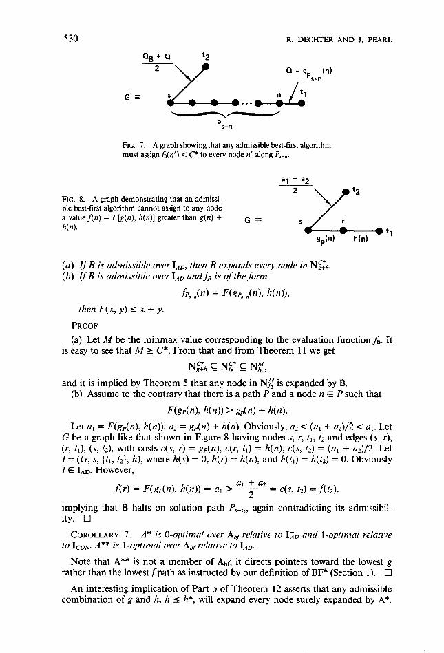
FIG. 7. A graph showing that any admissible best-first algorithm must assignfs(n’) < Cc to every node n’ along P,,.
a1 + a2 2
FIG. 8. A graph demonstrating that an admissi- ble best-first algorithm cannot assign to any node a valuef(n) = F[g(n), h(n)] greater than g(n) + GZ h(n).
S
s,(n) h(n)
(a) If B is admissible over I A~, then B expands every node in Ng$,. (b) If B is admissible over IAN and fB is of the form
fP,,@) = f’(gP&), h(n)), then F(x, y) 5 x + y.
PROOF (a) Let M be the minmax value corresponding to the evaluation function fB. It
is easy to see that M L C*. From that and from Theorem 11 we get
N$ !Z NT C Njf,
and it is implied by Theorem 5 that any node in Ng is expanded by B. (b) Assume to the contrary that there is a path P and a node n E P such that
F(gP(n), h(n)) > gh) + h(n).
Let al = F(gp(n), h(n)), a2 = gp(n) + h(n). Obviously, a2 < (a, + a2)/2 < al. Let G be a graph like that shown in Figure 8 having nodes s, r, tl, t2 and edges (s, r), (r, t,), (s, t2), with costs c(s, r) = gp(n), c(r, tl) = h(n), c(s, t2) = (al + a2)/2. Let Z= (G, s, (tl, t2), h), where h(s) = 0, h(r) = h(n), and h(t,) = h(t2) = 0. Obviously Z E IAD. However,
al + a2 f(r) = F(gp(n), h(n)) = al > - = 2 4% t2) = f(t21,
implying that B halts on solution path Ps+, again contradicting its admissibil- ity. Cl
COROLLARY 7. A* is O-optimal over Abf relative to IiD and l-optimal relative to ICON. A** is I -optimal over Abf relative to IAD.
Note that A** is not a member of Abf; it directs pointers toward the lowest g rather than the lowest f path as instructed by our definition of BF* (Section 1). •i
An interesting implication of Part b of Theorem 12 asserts that any admissible combination of g and h, h 5 h*, will expand every node surely expanded by A*.
Generalized BF Search Strategies and the Optimality ofA*
Class of Algorithms
531
Domain
Of
Problem
Instances
Admissible
‘AD
Admissible
and
non pathological
‘iD
Consistent
‘CON
Consistent
nonpathological
’ CON
Admissible
if h5h’
A ad
A” is 3-optimal
No P-optimal exists
A’ is P-optimal
No l-optimal exists
A’ is l-optimal A* is l-optimal A’ is l-optimal
No O-optimal exists No O-optimal exists No O-optimal exists
A’ is O-optimal A’ is O-optimal A* is O-optimal
Globally Compatible
with A’
Best-First
A’ is l-optimal A’ is l-optimal
No O-optimal exists No O-optimal exists
A’ is O-optimal A l is O-optimal
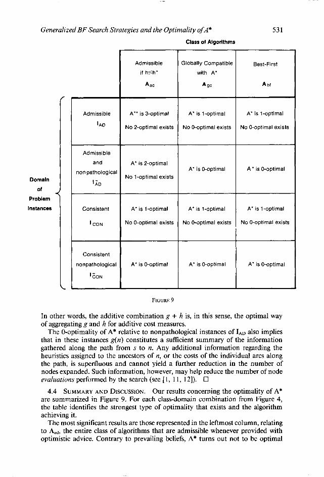
FIGURE 9
In other words, the additive combination g + h is, in this sense, the optimal way of aggregating g and h for additive cost measures.
The 0-optimality of A* relative to nonpathological instances of IAD also implies that in these instances g(n) constitutes a suffkient summary of the information gathered along the path from s to n. Any additional information regarding the heuristics assigned to the ancestors of n, or the costs of the individual arcs along the path, is superfluous and cannot yield a further reduction in the number of nodes expanded. Such information, however, may help reduce the number of node evaluations performed by the search (see [ 1, 11, 121). 0
4.4 SUMMARY AND DISCUSSION. Our results concerning the optimality of A* are summarized in Figure 9. For each class-domain combination from Figure 4, the table identifies the strongest type of optimality that exists and the algorithm achieving it.
The most significant results are those represented in the leftmost column, relating to Aad, the entire class of algorithms that are admissible whenever provided with optimistic advice. Contrary to prevailing beliefs, A* turns out not to be optimal
532 R. DECHTER AND J. PEARL
over Aad relative to every problem graph quantified with optimistic estimates. In some graphs, there are admissible algorithms that will find the optimal solution in just a few steps, whereas A* (as well as A** and all their variations) would be forced to explore arbitrary large regions of the search graphs (see Figure 6a). In bold defiance of the argument of Hart et al. [6] for the optimality of A*, these algorithms succeed in outsmarting A* by penetrating regions of the graph that A* finds unpromising (at least temporarily), visiting some goal nodes in these regions, then processing the information gathered to identify and purge those nodes on OPEN that no longer promise to sprout a solution better than the cheapest one at hand.
In nonpathological cases, however, these algorithms cannot outsmart A* without paying a price. The 2-optimality of A* relative to LD means that each such algorithm must always expand at least one node that A* will skip. This means that the only regions of the graph capable of providing node-purging information are regions that A* will not visit at all. In other words, A* makes full use of the information gathered along its search, and there could be no gain in changing the order of visiting nodes that A* plans to visit anyhow.
This instance-by-instance node trade-off no longer holds when pathological cases are introduced. The fact that A* is not 2-optimal relative to IAp means that some smart algorithms may outperform A* by simply penetrating certain regions of the graph earlier than A* (A* will later visit these regions), thus expanding only a proper subset of the set of nodes expanded by A*. In fact the lack of 2-optimality in the (Aad, IAD) entry of Figure 9 means that no algorithm can be protected against such smart competitors. For any admissible algorithm A,, there exists an- other admissible algorithm AZ and a graph G quantified by optimistic heuristic h( h 5 h*) such that A2 expands fewer nodes than Ai when applied to G. M&o [ 121 has recently shown that no optimal algorithm exists if complexity is measured by the number of expansion operations (a node can be reopened several times). Our result now shows that Aad remains devoid of an optimal algorithm even if we measure complexity by the number of distinct nodes expanded.
The type-3 optimality of A** over Aad further demonstrates that those “smart” algorithms that prevent A* from achieving optimality are not smart after all, but simply lucky; each takes advantage of the peculiarity of the graph for which it was contrived, and none can maintain this superiority over all problem instances. If it wins on one graph, there must be another where it is beaten, and by the very same opponent, A**. It is in this sense that A** is 3-optimal; it exhibits a universal robustness against all its challengers.
Perhaps the strongest claim that Figure 9 makes in favor of A* is contained in the entries related to ICON, the domain of problems in which h is known to be not only admissible, but also consistent. It is this domain that enables A* to unleash its full pruning powers, achieving a node-by-node superiority (types 0 and 1) over all admissible algorithms. Recalling also that, under consistent h, A* never reopens closed nodes and that only few nodes are affected by the choice of tie-breaking rule (see [ 16]), we conclude that in this domain A* constitutes the most effective scheme of utilizing the advice provided by h.
This optimality is especially significant in light of the fact that consistency is not an exception but rather a common occurrence; almost all admissible heuristics invented by people are consistent. The reason is that the technique people invoke in generating heuristic estimates is often that of relaxation: We imagine a simplified version of the problem at hand by relaxing some of its constraints and solve the relaxed version mentally; then we use the cost of the resulting solution as a heuristic
Generalized BF Search Strategies and the Optimality ofA* 533
for the original problem [ 151. It can be shown that any heuristic generated by such a process is automatically consistent, which explains the abundance of consistent cases among human-generated heuristics. Thus, the strong optimality of A* under the guidance of consistent heuristics implies, in effect, its optimality in most cases of practical interest.
Appendix A. Finding an t-Optimal Path in a Tree with Random Costs Let C*(N, p) be the optimal cost of a root-to-leaf path in a uniform binary tree of height N, where each branch independently has a cost of 1 or 0 with probability p and 1 - p, respectively. We wish to prove that for p > i
P[M 1 (1 -t c)c*(N, p)] --* 0 6 > 0,
where
M = mjn yz; Mn%
f(n) = g(n) + i*[N - d(n)],
and where (Y* is defined by the equation
Call a path P ((u, L)-regular if the cost of every successive path segment of length L along P is at most CYL. Karp and Pearl [9] have shown that
(a) P[C*(N, p) 5 cx1v] + 0 for a! < (Y*. (b) If (Y < (Y*, one can always find a constant L, such that the probability that
there exists an (CX, L,)-regular path of length N is bounded away from zero. Call this probability 1 - qa (qa < 1).
Consider the profile off along a ((Y, L)-regular path P sprouting from level do below the root. Along such a path g(n) satisfies
g(n) 5 do + [d(n) - d&x + CYL,
and, consequently,
f(n) 5 (1 - Ly)do + cu*N + aL + d(n)(a - a*).
For cr > (Y*, the expression on the right attains its maximum when d(n) reaches its largest value of N - do, and so
A4 I m&z) 5 (1 - 2a + a*)dg + CYL + NCY.
Now let do be any unbounded function of N such that do = o(N) and consider the probability P[M 2 (1 + 6)~y*Nj. For every (Y between (Y* and (1 + @a*, the inequality
(1 - 2~y + cy*)do(N) + CYL, + Ncu P (1 + 6)(r*N
will be satisfied for sufficiently large N, hence, choosing cr* < CY < (1 + ~)cY*, we have
P[M 2 (1 + 6)a*N] 5 P[no (a, L,)-regular path stems from level do(N)] % (432”“‘” --5, 0.
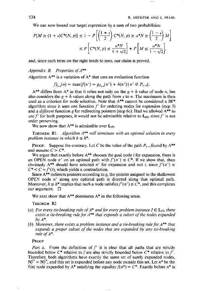
534 R. DECHTER AND J. PEARL
We can now bound our target expression by a sum of two probabilities:
P[M L (1 + t)C*(N, p)] I 1 - P
and, since each term on the right tends to zero, our claim is proved.
Appendix B. Properties of A** Algorithm A** is a variation of A* that uses an evaluation function
fk&) = maxIf = gp,Jn’> + b’) In’ E Pd.
A** differs from A* in that it relies not only on the g + h value of node n, but also considers the g + h values along the path from s to 12. The maximum is then used as a criterion for node selection. Note that A** cannot be considered a BF* algorithm since it uses one function f’ for ordering nodes for expansion (step 3) and a different function g for redirecting pointers (step 6~). Had we allowed A** to use f for both purposes, it would not be admissible relative to IAD, since f’ is not order preserving.
We now show that A** is admissible over IAb.
THEOREM B 1. Algorithm A** will terminate with an optimal solution in every problem instance in which h 5 h*.
PROOF. Suppose the contrary. Let C be the value of the path P,_, found by A** and assume C > C*.
We argue that exactly before A ** chooses the goal node t for expansion, there is an OPEN node n’ on an optimal path with f’(n’) 4 C*. If we show that, than obviously A** should have selected n’ for expansion and not t, since f’(n’) 5 C* < C = f (t), which yields a contradiction.
Since A** redirects pointers according to g, the pointer assigned to the shallowest OPEN node n’ along any optimal path is directed along that optimal path. Moreover, h c h* implies that such a node satisfiesf (n’) I C*, and this completes our argument. El
We next show that A** dominates A* in the following sense.
THEOREM B2
(a) For every tie-breaking rule of A* and for every problem instance I E IAD, there exists a tie-breaking rule for A ** that expands a subset of the nodes expanded by A*.
(b) Moreover, there exists a problem instance and a tie-breaking rule for A** that expands a proper subset of the nodes that are expanded by any tie-breaking rule of A*.
PROOF
Part a. From the definition off’ it is clear that all paths that are strictly bounded below C* relative to f are also strictly bounded below C* relative to f’. Therefore, both algorithms have exactly the same set of surely expanded nodes, N/c’= NF, and this set is expanded before any node outside this set. Let It* be the first node expanded by A* satisfying the equality f(n*) = C*. Exactly before n* is
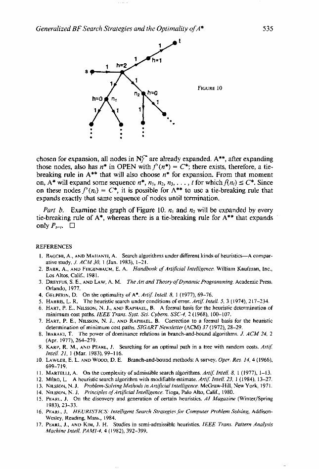
Generalized BF Search Strategies and the Optimality of A* 535
FIGURE 10
chosen for expansion, all nodes in N/c’ are already expanded. A**, after expanding those nodes, also has n* in OPEN withf(n*) = C*; there exists, therefore, a tie- breaking rule in A ** that will also choose n* for expansion. From that moment on, A* will expand some sequence n*, nl, n2, n3, . . . , t for whichf(ni) I C*. Since on these nodes f (rti) = C*, it is possible for A ** to use a tie-breaking rule that expands exactly that same sequence of nodes until termination.
Part b. Examine the graph of Figure 10. nI and n2 will be expanded by every tie-breaking rule of A*, whereas there is a tie-breaking rule for A** that expands only P,+ 0
REFERENCES
I. BAGCHI, A., AND MAHANTI, A. Search algorithms under different kinds of heuristics-A compar- ative study. J. ACM30, 1 (Jan. 1983), l-21.
2. BARR, A., AND FEIGENBAUM, E. A. Handbook of Artificial Intelligence. William Kaufman, Inc., Los Altos, Calif., 198 1.
3. DREYFUS, S. E., AND LAW, A. M. The Art and Theory ofDynamic Programming. Academic Press, Orlando, 1977.
4. GELPERIN, D. On the optimality of A*. Artij: Zntell. 8, 1 (1977), 69-76. 5. HARRIS, L. R. The heuristic search under conditions of error. ArtiJ: Intell. 5, 3 (1974), 217-234. 6. HART, P. E., NILSSON, N. J., AND RAPHAEL, B. A formal basis for the heuristic determination of
minimum cost paths. IEEE Trans. Syst. Sci. Cybern. SSC-4, 2 (1968), 100-107. 7. HART, P. E., NILSSON, N. J., AND RAPHAEL, B. Correction to a formal basis for the heuristic
determination of minimum cost paths. SIGART Newsletter (ACM) 37 (1972), 28-29. 8. IBARAKI, T. The power of dominance relations in branch-and-bound algorithms. J. ACM 24, 2
(Apr. 1977), 264-279. 9. KARP, R. M., AND PEARL, J. Searching for an optimal path in a tree with random costs. Artif:
Zntell. 21, I (Mar. 1983), 99-116. IO. LAWLER, E. L. AND WOOD, D. E. Branch-and-bound methods: A survey. Oper. Res. 14, 4 (1966),
699-719. I I. MARTELLI, A. On the complexity of admissible search algorithms. Artif: Intell. 8, 1 (1977), 1-13. 12. M~Ro, L. A heuristic search algorithm with modifiable estimate. Artif: Intell. 23, 1 (1984) 13-27. 13. NILSSON, N. J. Problem-Solving Methods in Artificial Intelligence. McGraw-Hill, New York, 197 1. 14. NILSSON, N. J. Principles ofArtijicia1 Intelligence. Tioga, Palo Alto, Calif., 1980. 15. PEARL, J. On the discovery and generation of certain heuristics. AI Magazine (Winter/Spring
1983), 23-33. 16. PEARL, J. HEURISTICS: Intelligent Search Strategies for Computer Problem Solving, Addison-
Wesley, Reading, Mass., 1984. 17. PEARL, J., AND KIM, J. H. Studies in semi-admissible heuristics. IEEE Trans. Pattern Analysis
Machine Intell. PAMI-4, 4 (1982), 392-399.
536 R. DECHTER AND J. PEARL
18. POHL, I. First results on the effect of error in heuristic search. Much. Intell. 5 (1969) 219-236. 19. POHL, I. Bi-directional search. In Machine Intelligence, vol. 6, B. Meltzer and D. Michie, Eds.
American Elsevier, New York, 1971, pp. 127-140. 20. POHL, I. The avoidance of (relative) catastrophe, heuristic competence, genuine dynamic weighting
and computational issues in heuristic problem solving. In Proceedings of the 3rd International Joint Conference on ArtiJicial Intelligence (Stanford, Calif., Aug. 20-23). William Kaufman, Inc., Los Altos, Calif., 1973.
RECEIVED MAY 1983; REVISED NOVEMBER 1984; ACCEPTED JANUARY 1985
Journal ofthe Association for Computing Machinery, Vol. 32, No. 3, July 1985.