Generalized gradient descent

Geoff Gordon & Ryan TibshiraniOptimization 10-725 / 36-725

1

Remember subgradient method

We want to solveminx∈Rn

f(x),

for f convex, not necessarily differentiable

Subgradient method: choose initial x(0) ∈ Rn, repeat:

x(k) = x(k−1) − tk · g(k−1), k = 1, 2, 3, . . .

where g(k−1) is a subgradient of f at x(k−1)

If f is Lipschitz on a bounded set containing its minimizer, thensubgradient method has convergence rate O(1/

√k)

Downside: can be very slow!

2

Outline

Today:

• Generalized gradient descent

• Convergence analysis

• ISTA, matrix completion

• Special cases

3

Decomposable functionsSuppose

f(x) = g(x) + h(x)

• g is convex, differentiable

• h is convex, not necessarily differentiable

If f were differentiable, gradient descent update:

x+ = x− t∇f(x)

Recall motivation: minimize quadratic approximation to f aroundx, replace ∇2f(x) by 1

t I,

x+ = argminz

f(x) +∇f(x)T (z − x) +1

2t‖z − x‖2︸ ︷︷ ︸

ft(z)

4

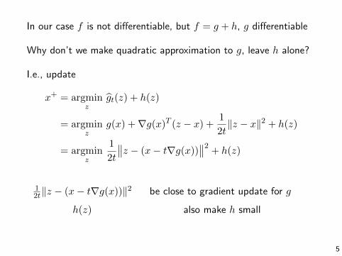
In our case f is not differentiable, but f = g + h, g differentiable

Why don’t we make quadratic approximation to g, leave h alone?

I.e., update

x+ = argminz

gt(z) + h(z)

= argminz

g(x) +∇g(x)T (z − x) +1

2t‖z − x‖2 + h(z)

= argminz

1

2t

∥∥z − (x− t∇g(x))∥∥2

+ h(z)

12t‖z − (x− t∇g(x))‖2 be close to gradient update for g

h(z) also make h small

5

Generalized gradient descent

Define

proxt(x) = argminz∈Rn

1

2t‖x− z‖2 + h(z)

Generalized gradient descent: choose initialize x(0), repeat:

x(k) = proxtk(x(k−1) − tk∇g(x(k−1))), k = 1, 2, 3, . . .

To make update step look familiar, can write it as

x(k) = x(k−1) − tk ·Gtk(x(k−1))

where Gt is the generalized gradient,

Gt(x) =x− proxt(x− t∇g(x))

t

6

What good did this do?

You have a right to be suspicious ... looks like we just swappedone minimization problem for another

Point is that prox function proxt(·) is can be computed analyticallyfor a lot of important functions h. Note:

• proxt doesn’t depend on g at all

• g can be very complicated as long as we can compute itsgradient

Convergence analysis: will be in terms of # of iterations of thealgorithm

Each iteration evaluates proxt(·) once, and this can be cheap orexpensive, depending on h

7

ISTAConsider lasso criterion

f(x) =1

2‖y −Ax‖2︸ ︷︷ ︸

g(x)

+.

.λ‖x‖1︸ ︷︷ ︸h(x)

Prox function is now

proxt(x) = argminz∈Rn

1

2t‖x− z‖2 + λ‖z‖1

= Sλt(x)

where Sλ(x) is the soft-thresholding operator,

[Sλ(x)]i =

xi − λ if xi > λ

0 if − λ ≤ xi ≤ λxi + λ if xi < −λ

8

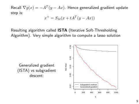
Recall ∇g(x) = −AT (y −Ax). Hence generalized gradient updatestep is:

x+ = Sλt(x+ tAT (y −Ax))

Resulting algorithm called ISTA (Iterative Soft-ThresholdingAlgorithm). Very simple algorithm to compute a lasso solution

Generalized gradient(ISTA) vs subgradient

descent:

0 200 400 600 800 1000

0.02

0.05

0.10

0.20

0.50

k

f(k)

−fs

tar

Subgradient methodGeneralized gradient

9

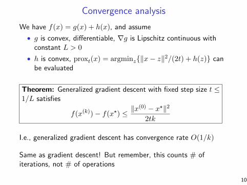
Convergence analysis

We have f(x) = g(x) + h(x), and assume

• g is convex, differentiable, ∇g is Lipschitz continuous withconstant L > 0

• h is convex, proxt(x) = argminz‖x− z‖2/(2t) + h(z) canbe evaluated

Theorem: Generalized gradient descent with fixed step size t ≤1/L satisfies

f(x(k))− f(x?) ≤ ‖x(0) − x?‖2

2tk

I.e., generalized gradient descent has convergence rate O(1/k)

Same as gradient descent! But remember, this counts # ofiterations, not # of operations

10

ProofSimilar to proof for gradient descent, but with generalized gradientGt replacing gradient ∇f . Main steps:

• ∇g Lipschitz with constant L ⇒

f(y) ≤ g(x) +∇g(x)T (y − x) +L

2‖y − x‖2 + h(y) all x, y

• Plugging in y = x+ = x− tGt(x),

f(x+) ≤ g(x)− t∇g(x)TGt(x) +Lt

2‖Gt(x)‖2 +h(x− tGt(x))

• By definition of prox,

x− tGt(x) = argminz∈Rn

1

2t‖z − (x− t∇g(x))‖2 + h(z)

⇒ ∇g(x)−Gt(x) + v = 0, v ∈ ∂h(x− tGt(x))

11

• Using Gt(x)−∇g(x) ∈ ∂h(x− tGt(x)), and convexity of g,

f(x+) ≤ f(z) +Gt(x)T (x− z)− (1− Lt

2)t‖Gt(x)‖2 all z

• Letting t ≤ 1/L and z = x?,

f(x+) ≤ f(x?) +Gt(x)T (x? − x)− t

2‖Gt(x)‖2

= f(x?) +1

2t

(‖x− x?‖2 − ‖x+ − x?‖2

)Proof proceeds just as with gradient descent.

12

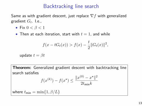
Backtracking line search

Same as with gradient descent, just replace ∇f with generalizedgradient Gt. I.e.,

• Fix 0 < β < 1

• Then at each iteration, start with t = 1, and while

f(x− tGt(x)) > f(x)− t

2‖Gt(x)‖2,

update t = βt

Theorem: Generalized gradient descent with backtracking linesearch satisfies

f(x(k))− f(x?) ≤ ‖x(0) − x?‖2

2tmink

where tmin = min1, β/L

13

Matrix completion

Given matrix A, m× n, only observe entries Aij , (i, j) ∈ Ω

Want to fill in missing entries (e.g., ), so we solve:

minX∈Rm×n

1

2

∑(i,j)∈Ω

(Aij −Xij)2 + λ‖X‖∗

Here ‖X‖∗ is the nuclear norm of X,

‖X‖∗ =

r∑i=1

σi(X)

where r = rank(X) and σ1(X), . . . σr(X) are its singular values

14

Define PΩ, projection operator onto observed set:

[PΩ(X)]ij =

Xij (i, j) ∈ Ω

0 (i, j) /∈ Ω

Criterion is

f(X) =1

2‖PΩ(A)− PΩ(X)‖2F︸ ︷︷ ︸

g(X)

+.

.λ‖X‖∗︸ ︷︷ ︸h(X)

Two things for generalized gradient descent:

• Gradient: ∇g(X) = −(PΩ(A)− PΩ(X))

• Prox function:

proxt(X) = argminZ∈Rm×n

1

2t‖X − Z‖2F + λ‖Z‖∗

15

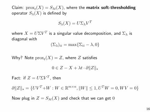
Claim: proxt(X) = Sλt(X), where the matrix soft-thresholdingoperator Sλ(X) is defined by

Sλ(X) = UΣλVT

where X = UΣV T is a singular value decomposition, and Σλ isdiagonal with

(Σλ)ii = maxΣii − λ, 0

Why? Note proxt(X) = Z, where Z satisfies

0 ∈ Z −X + λt · ∂‖Z‖∗

Fact: if Z = UΣV T , then

∂‖Z‖∗ = UV T+W : W ∈ Rm×n, ‖W‖ ≤ 1, UTW = 0,WV = 0

Now plug in Z = Sλt(X) and check that we can get 0

16

Hence generalized gradient update step is:

X+ = Sλt(X + t(PΩ(A)− PΩ(X)))

Note that ∇g(X) is Lipschitz continuous with L = 1, so we canchoose fixed step size t = 1. Update step is now:

X+ = Sλ(PΩ(A) + P⊥Ω (X))

where P⊥Ω projects onto unobserved set, PΩ(X) + P⊥Ω (X) = X

This is the soft-impute algorithm1, simple and effective methodfor matrix completion

1Mazumder et al. (2011), Spectral regularization algorithms for learninglarge incomplete matrices

17

Why “generalized”?

Special cases of generalized gradient descent, on f = g + h:

• h = 0 → gradient descent

• h = IC → projected gradient descent

• g = 0 → proximal minimization algorithm

Therefore these algorithms all have O(1/k) convergence rate

18

Projected gradient descent

Given closed, convex set C ∈ Rn,

minx∈C

g(x) ⇔ minx

g(x) + IC(x)

where IC(x) =

0 x ∈ C∞ x /∈ C

is the indicator function of C

Hence

proxt(x) = argminz

1

2t‖x− z‖2 + IC(z)

= argminz∈C

‖x− z‖2

I.e., proxt(x) = PC(x), projection operator onto C

19

Therefore generalized gradient update step is:

x+ = PC(x− t∇g(x))

i.e., perform usual gradient update and then project back onto C.Called projected gradient descent

−1.5 −1.0 −0.5 0.0 0.5 1.0 1.5

−1.

5−

1.0

−0.

50.

00.

51.

01.

5

c()

20

What sets C are easy to project onto? Lots, e.g.,

• Affine images C = Ax+ b : x ∈ Rn• Solution set of linear system C = x ∈ Rn : Ax = b• Nonnegative orthant C = x ∈ Rn : x ≥ 0 = Rn+• Norm balls C = x ∈ Rn : ‖x‖p ≤ 1, for p = 1, 2,∞• Some simple polyhedra and simple cones

Warning: it is easy to write down seemingly simple set C, and PCcan turn out to be very hard!

E.g., it is generally hard to project onto solution set of arbitrarylinear inequalities, i.e, arbitrary polyhedron C = x ∈ Rn : Ax ≤ b

21

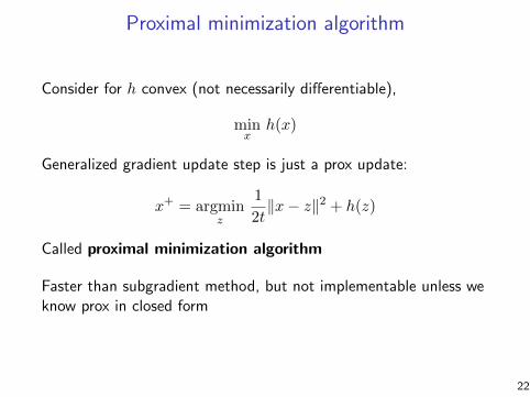
Proximal minimization algorithm

Consider for h convex (not necessarily differentiable),

minx

h(x)

Generalized gradient update step is just a prox update:

x+ = argminz

1

2t‖x− z‖2 + h(z)

Called proximal minimization algorithm

Faster than subgradient method, but not implementable unless weknow prox in closed form

22

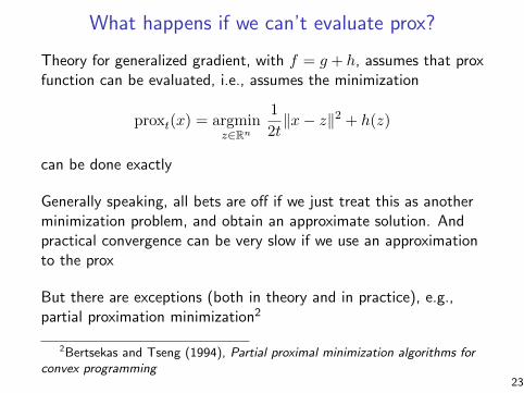
What happens if we can’t evaluate prox?

Theory for generalized gradient, with f = g + h, assumes that proxfunction can be evaluated, i.e., assumes the minimization

proxt(x) = argminz∈Rn

1

2t‖x− z‖2 + h(z)

can be done exactly

Generally speaking, all bets are off if we just treat this as anotherminimization problem, and obtain an approximate solution. Andpractical convergence can be very slow if we use an approximationto the prox

But there are exceptions (both in theory and in practice), e.g.,partial proximation minimization2

2Bertsekas and Tseng (1994), Partial proximal minimization algorithms forconvex programming

23

Almost cutting edge

We’re almost at the cutting edge for first order methods, but notquite ... still require too many iterations

Acceleration: use more than just x(k−1) to compute x(k) (e.g.,use x(k−2)), sometimes called momentum terms or memory terms

There are many different flavors of acceleration (at least three,mostly due to Nesterov)

Accelerated generalized gradient descent achieves optimal rateO(1/k2) among first order methods for minimizing f = g + h!

24

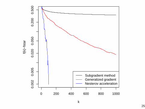
0 200 400 600 800 1000

0.00

20.

005

0.02

00.

050

0.20

00.

500

k

f(k)

−fs

tar

Subgradient methodGeneralized gradientNesterov acceleration

25

References

• E. Candes, Lecture Notes for Math 301, Stanford University,Winter 2010-2011

• L. Vandenberghe, Lecture Notes for EE 236C, UCLA, Spring2011-2012

26