Generalized higher-order nonlinear energy operators

1Tamr

wcdT

EfwoatcaAeAttsphsvmcg

Salzenstein et al. Vol. 24, No. 12 /December 2007 /J. Opt. Soc. Am. A 3717

Generalized higher-order nonlinearenergy operators

Fabien Salzenstein,1 Abdel-Ouahab Boudraa,2,* and Jean-Christophe Cexus2

1CNRS/Sciences et Technologies de l’Information et de la Communication-UPR 292, Université Louis PasteurLaboratoire Iness, 23, rue du Loess, BP20 CR-67037 Strasbourg Cedex 2, France

2Institut de Recherche de l’Ecole Navale, Ecole Navale/E3I2 (EA 3876) Ecole Nationale Supérieure des Ingénieursdes Etudes et Techniques d’Armement, Lanvéoc Poulmic, BP600, 29240 Brest–Armées, France

*Corresponding author: [email protected]

Received January 23, 2007; revised September 1, 2007; accepted September 10, 2007;posted September 28, 2007 (Doc. ID 79330); published November 19, 2007

We extend and generalize the Teager–Kaiser [in Proceedings of IEEE International Conference on Acoustics,Speech, and Signal Processing (1993), Vol. 3, p. 149] and the higher-order differential energy operators [IEEESignal Process. Lett. 2, 152 (1995)] to a large class of operators called higher-order energy operators. We showthat for AM-FM signal demodulation, the introduced partial derivative orders have to satisfy certain condi-tions. These operators are parameterized for local processing of AM-FM signals. The operators are illustratedusing synthetic signals and a real signal from light scanning interferometry. © 2007 Optical Society ofAmerica

OCIS codes: 100.0100, 260.0260.

Feaoaf

ddtopvtp

2Tbt�

Tcbaf=tle

. INTRODUCTIONhe Teager–Kaiser energy operator (TKEO) [1] is defineds a local energy measure for oscillating (simple har-onic) signals. This operator computes the energy of a

eal-valued signal x�t� as follows:

��x�t�� = �x�1��t��2 − x�0��t�x�2��t�, �1�

here x�k��t� denotes the kth derivative of x�t�. In the dis-rete case, the time derivatives are approximated by timeifferences. Thus, one discrete-time counterpart of theKEO becomes [2]

��x�n�� = x2�n� − x�n + 1�x�n − 1�. �2�

quation (2) shows that only three samples are requiredor the energy estimation at each time instant. This ishy the TKEO is qualified as an instantaneous energyperator. This excellent time resolution provides us withn ability to capture the signal energy fluctuations. Fur-hermore, this operator is very easy to implement effi-iently. The TKEO has found applications in speechnalysis [2], and in signal [3] and image processing [4,5].n interesting application lies in the field of interferom-try, where the luminance signals are approximated by anM-FM monocomponent model. In this way, the extrac-

ion of the envelope or the phase provides useful informa-ion, such as the position of the surface, in order to mea-ure the roughness of the structure. It is also possible torocess the two-component signals, combining differentigher-order operators [6]. For a monocomponent AM-FMignal, the TKEO is able to extract the instantaneous en-elope and frequency information [2]. Maragos and Pota-ianos [7] have proposed an extension of the TKEO,

alled the k-order differential energy operator (DEO) �k,iven by

1084-7529/07/123717-11/$15.00 © 2

�k�x�t�� = x�1��t�x�k−1��t� − x�0��t�x�k��t�. �3�

or k=2 the TKEO corresponds to the second-order differ-ntial energy operator. It is also possible to demodulaten AM-FM signal using this class of operators. A continu-us version of DEO has been extended to 2D signals (im-ges) to measure the surface shape of a material in inter-erence microscopy [5,8].

In this work a large class of continuous DEOs is intro-uced. A new formulation of this continuous DEO is intro-uced using higher-order partial derivatives with a con-inuous lag parameter � of the signal. This new family ofperators leads to more flexible operators in terms of sam-ling rate precision and computing time. Examples of en-elope and frequency detection, using the proposed opera-ors, of a noisy synthetic signal and a real one areresented.

. HIGHER-ORDER ENERGY OPERATORShe higher-order energy operator (HEO), �p,q,m,l�x�t��, isased on the four partial pth, qth, mth, and lth deriva-ives of a signal, x�t�, satisfying the condition p+q=m+ l,p ,q�� m , l�, and is defined as follows:

�p,q,m,l�x�t�� = x�p��t�x�q��t� − x�m��t�x�l��t�. �4�

he HEO measures the higher-order energies of a classi-al monocomponent harmonic oscillator (mass suspendedy a spring), which is subjected to a displacement of x�t�,nd normalized to half unit mass [7]. It is easy to see thator the derivative order combinations (p=1, q=k−1, m0, l=k) and (p=1, q=1, m=0, l=2), the HEO is reduced

o the DEO [7] and to the TKEO [1], respectively. The re-ations between the different orders lead to the followingquations:

007 Optical Society of America

wIw�ik

AIsx

wtfi

Tb

U

Tp

Tlc

BCn�acpfwcIt

T

Ut

w

�

Tw

3718 J. Opt. Soc. Am. A/Vol. 24, No. 12 /December 2007 Salzenstein et al.

��p,q,m,l

�t�x�t�� = �p+1,q,m+1,l�x�t�� + �p,q+1,m,l+1�x�t��,

�p,q,m,l�x�t�� = �p+1,q+1,m+1,l+1�x�t��,

here x�t� represents the first derivative of the signal x�t�.t is possible to unify the operators into k-order operators,here k=p+q=m+ l. To differentiate this operator fromk�x�t��, we denote it �Hk,p,m

�x�t��. It is important to keepn mind that �k corresponds to only one operator of order, while �Hk,p,m

is a set of operators of order k.

. Discretizing the Higher-Order Energy Operatorf we replace continuous derivatives of x�t� with a two-ample symmetric difference, the p-order derivative of�t� is a function of its �p−1�-order one,

x�p��nTs� =x�p−1��n + 1�Ts� − x�p−1��n − 1�Ts�

2Ts, �5�

here Ts is the sampling period. The system defined byhis difference [Eq. (5)] is a finite impulse response (FIR)lter where the frequency response is given by

H�z� =z − z−1

2Ts. �6�

hus, the p-order derivative can be rewritten using theinomial coefficient as follows:

X�p��z� = X�z�Hp�z� = X�z�1

�2Ts�p�k=0

k=p

Cpk�− 1�p−kzkzk−p,

=1

�2Ts�p�k=0

k=p

Cpk�− 1�p−kz2k−p. �7�

sing the Z-inverse transform we obtain

x�p��n� =1

�2Ts�p�k=0

k=p

Cpk�− 1�p−kx�n + 2k − p�. �8�

hus, the quantity Qk�x�n��=x�p��n�x�q��n�−x�m��n�x�l��n�rovides

Qk�x�n�� =1

�2Ts�k � ��i=0

i=p

�j=0

j=q

Cpi Cq

j �− 1�k−�i+j�

�x�n + 2i − p�x�n + 2j − q�

− �i=0

i=m

�j=0

j=l

Cmi Cl

j�− 1�k−�i+j�

�x�n + 2i − m�x�n + 2j − l�� . �9�

aking the most extreme samples in the expression (9)eads to the following higher-order symmetric and dis-rete operator denoted by � d :
Hk,p,m
k even:

�Hk,p,md �x�n�� =

1

2�x�n + p�x�n + q� + x�n − p�x�n − q�

− �x�n + m�x�n + l� + x�n − m�x�n − l��,

�10�

k odd:


1

2�x�n + m�x�n + l� + x�n − m�x�n − l�

− �x�n + p�x�n + q� + x�n − p�x�n − q��.

�11�

. Continuous Demodulationonsider the demodulation problem of a real AM-FM sig-al, x�t�=a�t�cos��t�t+��, into its amplitude envelope

a�t�� and instantaneous frequency (IF) ��t�. We make thessumption that a�t� and ��t� do not vary too fast (rate ofhange) or too greatly (range of value) with time com-ared to the carrier frequency of x�t� [9,10]. Thus, locally,or the short time interval, J= �t1 , t2� where �t2− t1��T,e can make the approximation that a�t0�A and ��t0��, t0�J. T is the signal duration. In this case x�t� is lo-

ally approximated by a pure sinusoid, x�t�=A cos��t+��.t is easy to see that the pth derivative of x�t� can be writ-en as

x�p��t0� = A�p cos�t0 + � +�

2p� .

he output of �Hk,p,mfor x�t0� is given by

�Hk,p,m�x�t0�� =

A2�k

2 �cos�p − q��

2� − cos�m − l��

2�� .

�12�

sing a trigonometric identity, relation (12) can be writ-en as

�Hk,p,m�A cos��t0 + �� = A2�k sin�

4c�sin�

4b� ,

�13�

here

c = p − q + m − l = 2�m + p − k�,

b = q − p + m − l = 2�m − p�. �14�

Hk,p,moutput of x�t0� is given by

�Hk,p,m�x�t0�� = �Hk,p,m

�A� cos��t0 + � + �/2��, �15�

=A2�k+2 sin�

4c�sin�

4b� . �16�

hus, provided that sin�� /4�c�sin�� /4�b��0 one canrite

Lp

w

F

AtT�1otsd

Futt

CL=

F

w

�

I

Too(fnb

�

I

FI

I[

Fta


�Hk,p,m�x�t0��

�Hk,p,m�x�t0��

=A2�k+2 sin��/4�c�sin��/4�b�

A2�k sin��/4�c�sin��/4�b�= �2.

�17�

et us consider now the parameters �p1 ,q1 ,m1 , l1� so that1+q1=m1+ l1=2k:

�H2k,p1,m1�A cos��t0 + �� = A2�2k sin�

4c1�sin�

4b1� ,

�18�

here

c1 = p1 − q1 + m1 − l1 = 2�m1 + p1 − 2k�,

b1 = q1 − p1 + m1 − l1 = 2�m1 − p1�. �19�

inally, Eqs. (13) and (18) yield

�Hk,p,m

2 �x�t0��

�H2k,p1,m1�x�t0��

=A4�2k sin2��/4�c�sin2��/4�b�

A2�2k sin��/4�c1�sin��/4�b1�,

= A2sin2��/4�c�sin2��/4�b�

sin��/4�c1�sin��/4�b1�. �20�

ccording to Eq. (13) in order to estimate the product ofhe amplitude, A, and the IF, �, by �Hk,p,m

, as for theKEO [2], the factors �sin�� /4�c�sin�� /4�b�� and

sin�� /4�c1�sin�� /4�b1�� must approximately be equal to. A usual way that this can happen is when the amountf modulation is small and the bandwidths of the ampli-ude and the frequency modulating signals are muchmaller than the carrier frequency [4]. Under these con-itions, detailed in proposition 1 (see Subsection 2.E):

�Hk,p,m

2 �x�t0��

�H2k,p1,m1�x�t0��

A2. �21�

or different short intervals J�T, � and A are calculatedsing relations (17) and (21), respectively. For an estima-ion of the envelope and the IF, over the interval T, of x�t�he following relations are used:

�2�t� �Hk,p,m

�x�t��

�Hk,p,m�x�t��

, �22�

a2�t� �Hk,p,m

2 �x�t��

�H2k,p1,m1�x�t��

. �23�

. Discrete Demodulationet a real-valued signal be x�n�=A cos��n+�� with ��Ts. For p and q integers we have

x�n + p�x�n + q� =A2

2�cos�2�n + �k + 2�� + cos�p − q��.

�24�

or k-order even, the output of � gives
Hk,p,m

A2

2�cos�p − q�� − cos�m − l��,

= A2 sinb�

2 �sinc�

2 � , �25�

here b=q−p+m− l and c=p−q+m− l. Since

b = 2�m − p�, c = 2�m + p − k�,

Hk,p,mapplied to x�n� gives

�Hk,p,md �x�n�� = A2 sin��m − p��sin��m + p − k��.

�26�

n similar fashion, for k-order odd we have


A2

2�cos�m − l�� − cos�p − q��, �27�

=A2 sin��p − m��sin��m + p − k��.

�28�

he interest of such formulation is the relative robustnessf �Hk,p,m

against noise. Indeed, contrary to the continu-us version [Eq. (13)], in the discrete version [Eqs. (26) or28)] there is no multiplicative frequency term, �k. Thisrequency factor may contain some high-frequency compo-ents of the noise. If we replace the derivative of x�t� withackward difference, x1�n�=x�n�−x�n−1�, we obtain

x1�n� A�cos��n + �� − cos��n − 1� + ��, �29�

=− 2A sin��/2�sin��n − 0.5� + ��. �30�

Hk,p,m(k even) applied to x1�n� gives

�Hk,p,md �x1�n�� = 4A2 sin2�

2 �sinb�

2 �sinc�

2 � . �31�

f sin�� /2�� /2 then

�Hk,p,md �x1�n�� A2�2 sinb

�

2 �sinc�

2 � . �32�

inally, for discrete �Hk,p,m, estimation of envelopes and

Fs is given by relations (33) and (34):

�2 =�Hk,p,m

d �x1�n��

�Hk,p,md �x�n��

, �33�

A =� �Hk,p,md �x�n��

sin��m − p��sin��m + p − k��. �34�

n this work we compare the discrete operators �Hk,p,mEq. (10)] with those of Maragos and Potamianos [7]:

km�x�n�� = x�n�x�n + k� − x�n − m�x�n + m + k�. �35�

or carrier frequency small compared to the Ts, estima-ion of envelopes and IFs by km is given by relations (36)nd (37):

N=bo=

DO

Tt

F

T

Tnkepea

ELqt�+vAe

co

S�+==cdtt

ts

Noa

FIflkl

L

woaaf

Tac=

GU=T

Rt

Uw


�2 =km�x1�n��

km�x�n��, �36�

A =� km�x�n��

sin�m��sin��m + k��. �37�

ote that for the operator [Eq. (35)], values k=0 and m1 give the TKEO. Comparative study of operators giveny Eq. (35) has been done in [4]. Only the most efficientperators corresponding to �k ,m�= �0,1� and �k ,m��2,1� are studied in this work.

. Orders Selection of the Filtersrders are selected such that

sinb�

2 �sinc�

2 � 1. �38�

his condition introduces some constraints on Ts and onhe integers b and c:

b� = �2k1 + 1��, c� = �2k2 + 1��. �39�

or k even we have

2�m − p�� = �2k1 + 1��, 2�m + p − k�� = �2k2 + 1��.

�40�

hus,

m − p

m + p − k=

2k1 + 1

2k2 + 1. �41�

his ratio shows that the choice of odd numerator and de-ominator is compatible with relation (38). Note that theorder must be even. Furthermore, since �Hk,p,m

is an en-rgy operator, the quantities [Eqs. (26) and (28)] must beositive, and consequently m must be greater than p. Forxample, the TKEO corresponds to order 2 �k=2� and thessociated integers are p=q=1, m=2, and l=0.

. Demodulation Conditionset us now write the conditions for envelope and fre-uency detections. According to Eq. (14), in order to havehe sinusoidal product of Eq. (13) equal to 1, �m−p� andm+p−k� should be odd integers of the form �m−p�=2n11 and �m+p−k�=2n2+1. Thus, we find that k is an evenalue given by k=2�n1−n2+p�. Thus, to demodulate anM-FM signal the orders of the continuous operators areven [10].

Proposition 1. For a continuous k-order operator, theondition that both p and m cannot be simultaneously oddr even is necessary.

Proof. Suppose that m=2m1 and p=2p1 (even integers).ince k is even, it can be written as k=2k1. Thus,m−p�+ �m+p−k�=2m−k=2n1+2n2+2⇒m=k1+n1+n21=2m1 and �m+p−k�− �m−p�=2p−k=2�n2−n1�⇒pn2−n1+k1=2p1. These two relations give 2�n2+k1�+12�p1+m1�, which is false. The demonstration for the oddase is obtained in a similar fashion. In conclusion, the or-er of these operators must be even with the conditionhat p and m or q and l are not odd or even at the sameime. This introduces some restrictions on the choice of

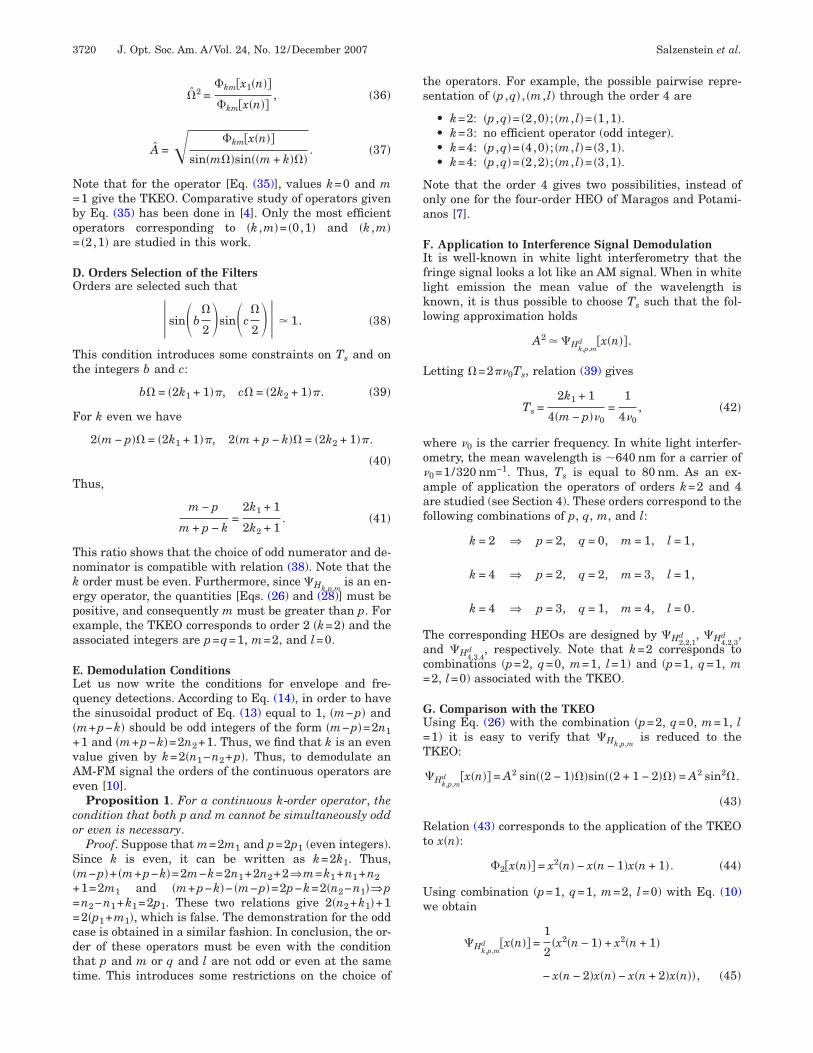
he operators. For example, the possible pairwise repre-entation of �p ,q� , �m , l� through the order 4 are

• k=2: �p ,q�= �2,0� ; �m , l�= �1,1�.• k=3: no efficient operator (odd integer).• k=4: �p ,q�= �4,0� ; �m , l�= �3,1�.• k=4: �p ,q�= �2,2� ; �m , l�= �3,1�.

ote that the order 4 gives two possibilities, instead ofnly one for the four-order HEO of Maragos and Potami-nos [7].

. Application to Interference Signal Demodulationt is well-known in white light interferometry that theringe signal looks a lot like an AM signal. When in whiteight emission the mean value of the wavelength isnown, it is thus possible to choose Ts such that the fol-

owing approximation holds

A2 �Hk,p,md �x�n��.

etting �=2�0Ts, relation (39) gives

Ts =2k1 + 1

4�m − p�0=

1

40, �42�

here 0 is the carrier frequency. In white light interfer-metry, the mean wavelength is �640 nm for a carrier of0=1/320 nm−1. Thus, Ts is equal to 80 nm. As an ex-mple of application the operators of orders k=2 and 4re studied (see Section 4). These orders correspond to theollowing combinations of p, q, m, and l:

k = 2 ⇒ p = 2, q = 0, m = 1, l = 1,

k = 4 ⇒ p = 2, q = 2, m = 3, l = 1,

k = 4 ⇒ p = 3, q = 1, m = 4, l = 0.

he corresponding HEOs are designed by �H2,2,1d , �H4,2,3

d ,nd �H4,3,4

d , respectively. Note that k=2 corresponds toombinations (p=2, q=0, m=1, l=1) and (p=1, q=1, m2, l=0) associated with the TKEO.

. Comparison with the TKEOsing Eq. (26) with the combination (p=2, q=0, m=1, l1) it is easy to verify that �Hk,p,m

is reduced to theKEO:

�Hk,p,md �x�n�� = A2 sin��2 − 1��sin��2 + 1 − 2�� = A2 sin2�.

�43�

elation (43) corresponds to the application of the TKEOo x�n�:

2�x�n�� = x2�n� − x�n − 1�x�n + 1�. �44�

sing combination (p=1, q=1, m=2, l=0) with Eq. (10)e obtain


1

2�x2�n − 1� + x2�n + 1�

− x�n − 2�x�n� − x�n + 2�x�n��, �45�

Ws

3EArefi

Lt

Ca

wPodoHr�

Ntn

Umli

Ciastsaaw

Ttpssom

ptp

Uc

Fopesr


=1

2�2�x�n − 1�� + 2�x�n + 1��. �46�

e find a propriety of the TKEO applied to a sinusoidalignal:

2�x�n�� =2�x�n − 1�� + 2�x�n + 1��

2. �47�

. PARAMETERIZED HIGHER-ORDERNERGY OPERATORs in [11] the HEO is generalized by introducing a lag pa-ameter �. This new class of operators is called param-terized HEO (PHEO). The PHEO, noted �PHk,�,p,m

, is de-ned as follows:

�PHk,�,p,m�x�t�� =

1

2�x�p��t + �/2�x�q��t − �/2�

+ x�p��t − �/2�x�q��t + �/2�

− �x�m��t + �/2�x�l��t − �/2�

+ x�m��t − �/2�x�l��t + �/2��.

et �xy�� ; t� be the instantaneous cross correlation be-ween x�t� and y�t�:

�xy��;t� = xt −�

2�yt +�

2� .

onsider the transformation PHk,�,p,m�x�t��, which associ-

tes to x�t� the relation

PHk,�,p,m�x�t�� = �x�p�x�q��;t� + �x�p�x�q��− �;t�

− �x�m�x�n��;t� − �x�m�x�n��− �;t�, �48�

here m+n=p+q. Thus, PHk,�,p,mmay be viewed as

HEO applied to random processes. In this work we limiturselves to deterministic signals. Thus, PHk,�,p,m

is re-uced to �PHk,�,p,m

. For �=0 and appropriate combinationsf the orders �p ,q ,m , l�, the operators TKEO, DEO, andEO can easily be deduced from the PHEO. Using the

easoning with the same assumptions as for the HEO, thePHk,�,p,m

outputs for x�t0� and x�t0� are given by

�PHk,�,p,m�x�t0�� = A2��

k cos��sin�

4c�sin�

4b�,

�PHk,�,p,m�x�t0�� = A2��

k+2 cos��sin�

4c�sin�

4b� .

ote that for each lag, �, corresponds an IF, ��. Providedhat cos��sin�� /4�c�sin�� /4�b��0, in the same man-er as in Subsection 2.B, one can write

�PHk,�,p,m�x�t0��

�PHk,�,p,m�x�t0��

=A2��

k+2 cos��sin��/4�c�sin��/4�b�

A2��k cos��sin��/4�c�sin��/4�b�

,

= ��2, �49�

�PHk,�,p,m

2 �x�t0��

�PH2k,�,p1,m1�x�t0��

=A4��

2k cos2��sin2��/4�c�sin2��/4�b�

A2��2k cos��sin��/4�c1�sin��/4�b1�

= A2 cos��sin2��/4�c�sin2��/4�b�

sin��/4�c1�sin��/4�b1�. �50�

nder the assumption �cos�� =1, it is possible to de-odulate an AM-FM signal. When � takes its values in a

ocal interval around t0, we have the property of periodic-ty:

� =n�

2��

, n integer ⇒ �PHk,�,p,m= �PHk,0

. �51�

onsequently, for a given even order, we are able to find,n theory, many operators to extract locally the envelopend the IF of an AM-FM signal. However, condition (51)upposes that the IF is known before applying our opera-ors. As for the HEO, A� and �� are estimated in eachhort interval J�T to have an estimation of the envelopend the IF, over the interval T, of x�t�. Again under thessumptions �sin�a� /4�sin�b� /4� � 1 and �cos�� 0e deduce

��2�t�

�PHk,�,p,m�x�t��

�PHk,�,p,m�x�t��

, �52�

a�2�t�

1

�cos��t��

�PHk,�,p,m

2 �x�t��

��PH2k,�,p1,m1�x�t��

. �53�

hus, it is possible to extract the envelope and above all,he IF independently of the current parameter �. It is ex-ected that the estimation of instantaneous envelope beensitive for very noisy data. Moreover, even the proposedolution takes theoretically into account the neighborhoodf each sample for any �, it is also expected that the esti-ation can be biased for very high � value.A possible solution to this problem is to oversample the

rocessed signal and then average the estimated ampli-udes and/or frequencies. To improve the robustness, weropose to average ��t� for different � values:

��t� =1

T�0

T

��t�d�. �54�

sing ��t� we re-estimate the envelope [Eq. (53)]. Identi-ally, the estimated envelopes are averaged as

a�t� =1

T�0

T

a��t�d�. �55�

or oversampled data, we set T to 1/d, where d is theversampling factor. The same approach can also be ap-lied for the nonparameterized methods by averaging thestimated values inside a window of size d. The over-ampled parameterized and nonparameterized algo-ithms are called, respectively, OS-PHEO and OS-HEO.

4Rpro2ae[

A

1Fftcea=tmsefmpccbAtanaTvs�Tmt

tQ2es1

2A54ae5ece

O

�

�

�

F

Fa

F(


. RESULTSesults of envelope and frequency detections by the pro-osed energy operators are illustrated on synthetic andeal signals. For synthetic signal, detection is performedn clean and noisy (ratio standard deviation–amplitude of% and 4%) signals. We focus our attention on the case ofn AM signal that is a sinusoid modulated by a dampedxponential. We compare the discrete operators �Hk,p,m

d

Eq. (10)] with those of Maragos and Potamianos [7].

. Discrete Operators

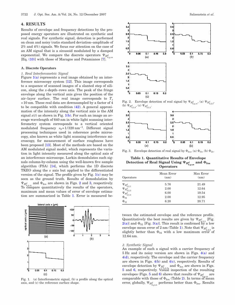
. Real Interferometric Signaligure 1(a) represents a real image obtained by an inter-

erence microscopy system [12]. This image correspondso a sequence of scanned images of a slanted step of sili-on, along the x-depth–rows axis. The peak of the fringenvelope along the vertical axis gives the position of their–layer surface. The real image corresponds to Ts10 nm. These real data are downsampled by a factor of 4

o be compatible with condition (42). A general approxi-ation of the intensity along the vertical axis is the AM

ignal x�t� as shown in Fig. 1(b). For such an image an av-rage wavelength of 640 nm in white light scanning inter-erometry system corresponds to a vertical orientedodulated frequency 0=1/320 nm−1. Different signal

rocessing techniques used in coherence probe micros-opy, also known as white light scanning interference mi-roscopy, for measurement of surface roughness haveeen proposed [13]. Most of the methods are based on theM modulated signal model, which represents the varia-

ion in light intensity measured along the optical axis ofn interference microscope. Larkin demodulates such sig-als column-by-column using the well-known five samplelgorithm (FSA) [14], which performs the 1D discreteKEO along the x axis but applied to the differentiatedersion of the signal. The profile given by Fig. 1(c) may beeen as the ground truth. Results of demodulation byHk,p,m

d and km are shown in Figs. 2 and 3, respectively.o compare quantitatively the results of the operators,aximum and mean values of error of envelope estima-

ion are summarized in Table 1. Error is measured be-

ig. 1. (a) Interferometric signal, (b) a profile along the opticalxis, and (c) the reference surface shape.

ween the estimated envelope and the reference profile.uantitatively the best results are given by �H4,2,3

d [Fig.(a)] and 01 [Fig. 3(a)]. This result is confirmed by a lownvelope mean error of 2 nm (Table 1). Note that �H4,2,3

d islightly better than 01 with a low maximum error of2.64 nm.

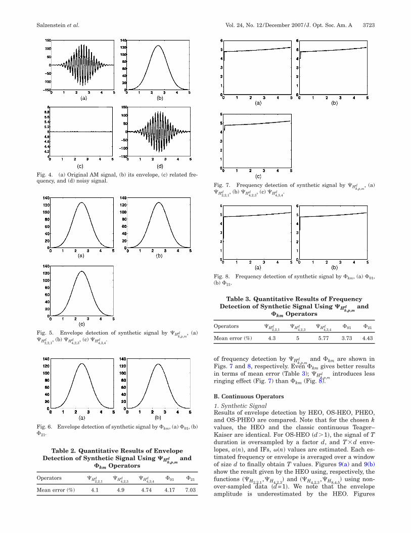
. Synthetic Signaln example of such a signal with a carrier frequency ofHz and its noisy version are shown in Figs. 4(a) and(d), respectively. The envelope and the carrier frequencyre shown in Figs. 4(b) and 4(c), respectively. Results ofnvelope detection by �Hk,p,m

d and km are shown in Figs.and 6, respectively. Visual inspection of the resulting

nvelopes (Figs. 5 and 6) shows that results of �Hk,p,md are

omparable with those of km (Table 2). In terms of meanrror, globally, � d performs better than . Results

Table 1. Quantitative Results of EnvelopeDetection of Real Signal Using �Hk,p,m

d and �kmOperators

peratorsMean Error

(nm)Max Error

(nm)

H2,2,1d 5.76 21.49

H4,2,3d 2.00 12.64

H4,3,4d 6.00 19.54

01 2.00 12.95

21 6.20 20.71

ig. 3. Envelope detection of real signal by km, (a) 01, (b) 21.

ig. 2. Envelope detection of real signal by �Hk,p,md , (a) �H4,2,3

d ,b) �H4,3,4

d , (c) �H2,2,1d .

Hk,p,m km

oFir

B

1RavKdltosfoa

O

M

O

MF�H2,2,1

, (b) �H4,2,3, (c) �H4,3,4

.

F21.

F�

F(

Fquency, and (d) noisy signal.


f frequency detection by �Hk,p,md and km are shown in

igs. 7 and 8, respectively. Even km gives better resultsn terms of mean error (Table 3); �Hk,p,m

d introduces lessinging effect (Fig. 7) than km (Fig. 8).

. Continuous Operators

. Synthetic Signalesults of envelope detection by HEO, OS-HEO, PHEO,nd OS-PHEO are compared. Note that for the chosen kalues, the HEO and the classic continuous Teager–aiser are identical. For OS-HEO �d�1�, the signal of Turation is oversampled by a factor d, and T�d enve-opes, a�n�, and IFs, ��n� values are estimated. Each es-imated frequency or envelope is averaged over a windowf size d to finally obtain T values. Figures 9(a) and 9(b)how the result given by the HEO using, respectively, theunctions ��H2,2,1

,�H4,2,3� and ��H4,2,3

,�H8,4,5� using non-

ver-sampled data �d=1�. We note that the envelopemplitude is underestimated by the HEO. Figures

Table 3. Quantitative Results of FrequencyDetection of Synthetic Signal Using �Hk,p,m

d and�km Operators

perators �H2,2,1d �H4,2,3

d �H4,3,4d 01 21

ean error (%) 4.3 5 5.77 3.73 4.43

ig. 7. Frequency detection of synthetic signal by �Hk,p,md , (a)

H2,2,1d , (b) �H4,2,3

d , (c) �H4,3,4d .

ig. 8. Frequency detection of synthetic signal by km, (a) 01,b) 21.

Table 2. Quantitative Results of EnvelopeDetection of Synthetic Signal Using �Hk,p,m

d and�km Operators

perators �H2,2,1d �H4,2,3

d �H4,3,4d 01 21

ean error (%) 4.1 4.9 4.74 4.17 7.03

ig. 5. Envelope detection of synthetic signal by �Hk,p,md , (a)

d d d

ig. 6. Envelope detection of synthetic signal by km, (a) 01, (b)

ig. 4. (a) Original AM signal, (b) its envelope, (c) related fre-

1=tdsnstbsasaase1[

samvt1sbatHectct

Fp

F(H

Fp

F(=

Fp=

Fp=


0(a)–10(d) show the result of the HEO approach for k�2,4� and k= �4,8� using an oversampling factor, respec-

ively, of d=5 and 10. The envelope amplitude is not un-erestimated. This result shows a link between the over-ampling and the estimation: the oversampled signal isaturally close to the continuous one. However, due touccessive derivatives, the lower the order k, the betterhe estimation. Actually, for parameters k= �4,8� the com-ination of the higher-order derivative value, the over-ampling, and the spline functions provide some ripplesround the maximum of the envelope [Fig. 10(d)]. In theame way, we note for PHEO an underestimation of themplitude without oversampling [Figs. 11(a) and 11(b)];nd a corrected level provided by oversampled data, re-pectively, with d=5 and 10 [Figs. 12(a)–12(d)]. A carefulxamination of the detected envelopes shown in Figs.0(a), 10(b), 13(a), and 13(b), and the original envelopeFig. 4(b)] shows that the OS-HEO and the HEO give the

ig. 9. Envelope detection of synthetic signal with an oversam-ling factor d=1 using (a) HEO, k= �2,4�; (b) HEO, k= �4,8�.

ig. 10. Envelope detection with an oversampling factor d=5:a) HEO, k= �2,4�; (b) HEO, k= �4,8�; d=10: (c) HEO, k= �2,4�; (d)EO, k= �4,8�.

ig. 11. Envelope detection of synthetic signal with an oversam-ling factor d=1 using (a) PHEO, k= �2,4�; (b) PHEO, k= �4,8�.

ame result for an oversampling factor d=5. Figures 13(a)nd 13(b) show the detection envelope using the OS-HEOethod for k= �2,4� and �4,8�. The � parameter takes its

alues in the range �−T ,T� with T=5. A careful examina-ion of the detected envelopes shown in Figs. 12(a), 12(b),4(a), and 14(b), and the original envelope [Fig. 4(b)]hows that the OS-PHEO and the PHEO have the sameehavior for an oversampling factor d=5. These resultsre confirmed by the error rates reported in Table 4. Thisable compares the error rate of the HEO, PHEO, OS-EO, OS-PHEO, and the Hilbert transform for two differ-

nt window sizes (applying the OS-PHEO). The rates de-rease with the oversampling. The error rate provided byhe PHEO method for d=1 (33.21%) versus d=5 (3.40%)onfirms the previous assumptions. One can notice thathe OS-PHEO provides the best results without oversam-

ig. 12. Envelope detection with an oversampling factor d=5:a) PHEO, k= �2,4�; (b) PHEO, k= �4,8�; d=10: (c) PHEO, k�2,4�; (d) PHEO, k= �4,8�.

ig. 13. Envelope detection of synthetic signal with an oversam-ling factor d=5 using (a) OS-HEO, k= �2,4�; (b) OS-HEO, k�4,8�.

ig. 14. Envelope detection of synthetic signal with an oversam-ling factor d=5 using (a) OS-PHEO, k= �2,4�; (b) OS-PHEO, k�4,8�.

piaed(ppotmcsPwHlmn

�

fsttt1rinadfni

OT

HPOOH

OT

HPOOH

Fs

F(H

OT

HPOOH

Fsk


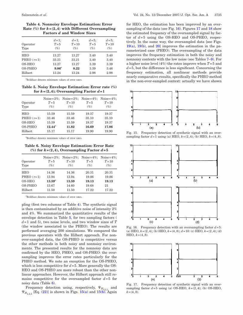
ling (first two columns of Table 4). The synthetic signals then contaminated by an additive noise of intensity 2%nd 4%. We summarized the quantitative results of thenvelope detection in Table 5, for two sampling factors (=1 and 5), two noise levels, and two window sizes of T

the window associated to the PHEO). The results areerformed averaging 200 simulations. We compared therevious operators with the Hilbert approach. For non-ver-sampled data, the OS-PHEO is competitive versushe other methods in both noisy and nonnoisy environ-ents. The presented results for the nonnoisy data are

onfirmed by the HEO, PHEO, and OS-PHEO: the over-ampling improves the error rates particularly for theHEO method. We note an exception for the OS-PHEO,hich is less competitive for d=5. More generally the OS-EO and OS-PHEO are more robust than the other non-

inear approaches. However, the Hilbert approach still re-ains competitive for the oversampled factor d=5 foroisy data (Table 6).Frequency detection using, respectively, �H2,2,1

and[Eq. (22)] is shown in Figs. 15(a) and 15(b). Again

Table 5. Noisy Envelope Estimation: Error rate (%)for k= „2,4…; Oversampling Factor d=1

peratorype

Noise=2%;T=5(%)

Noise=2%;T=10

(%)

Noise=4%;T=5(%)

Noise=4%;T=10

(%)

EO 15.59 15.59 19.37 19.37HEO ��=1� 33.46 33.46 35.10 35.10S-HEO 15.59 15.59 19.37 19.37S-PHEO 12.44a 11.82 16.69 17.06ilbert 15.17 15.17 19.90 19.90

aBoldface denotes minimum values of error rates.

Table 6. Noisy Envelope Estimation: Error Rate(%) for k= „2,4…, Oversampling Factor d=5

peratorype

Noise=2%;T=5(%)

Noise=2%;T=10

(%)

Noise=4%;T=5(%)

Noise=4%;T=10

(%)

EO 14.36 14.36 20.31 20.31HEO ��=1� 13.94 13.94 19.86 19.86S-HEO 13.59a 13.59 19.13 19.13S-PHEO 13.67 14.60 19.68 21ilbert 11.50 11.50 17.22 17.22


Table 4. Nonnoisy Envelope Estimation: ErrorRate (%) for k= „2,4… with Different Oversampling

Factors d and Window Sizes

peratorype

d=1;T=5(%)

d=1;T=10

(%)

d=5;T=5(%)

d=5;T=10

(%)

EO 13.27 13.27 3.40 3.40HEO ��=1� 33.21 33.21 3.40 3.40S-HEO 13.27 13.27 3.39 3.39S-PHEO 9.86a 8.22 3.39 3.46ilbert 13.24 13.24 2.98 2.98


H4,2,3

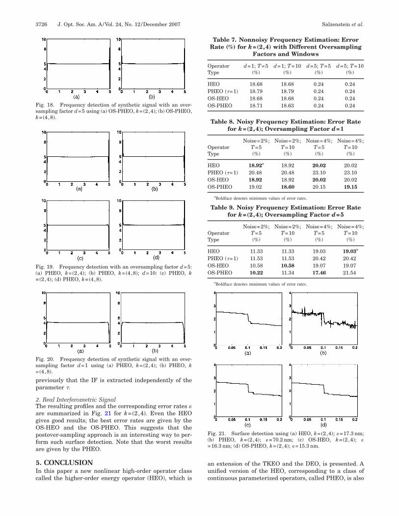
or HEO, the estimation has been improved by an over-ampling of the data (see Fig. 16). Figures 17 and 18 showhe estimated frequency of the oversampled signal by fac-or of d=5 using the OS-HEO and OS-PHEO, respec-ively. In the same way, the oversampled data [see Figs.9(a), 19(b), and 20] improves the estimation in the pa-ameterized case (PHEO). The oversampling of the datamproves the frequency estimation in both the noisy andonnoisy contexts with the low noise (see Tables 7–9). Forhigher noise level (4%) the rates improve when T=5 and=5, but the difference is less significant. Concerning the

requency estimation, all nonlinear methods provideearly comparative results, specifically the PHEO method

n the non-over-sampled context: actually we have shown

ig. 15. Frequency detection of synthetic signal with an over-ampling factor d=1 using (a) HEO, k= �2,4�; (b) HEO, k= �4,8�.

ig. 16. Frequency detection with an oversampling factor d=5:a) HEO, k= �2,4�; (b) HEO, k= �4,8�; d=10: (c) HEO, k= �2,4�; (d)EO, k= �4,8�.

ig. 17. Frequency detection of synthetic signal with an over-ampling factor d=5 using (a) OS-HEO, k= �2,4�; (b) OS-HEO,= �4,8�.

pp

2TagOpfa

5Ic

auc

OT

HPOO

OT

HPOO

OT

HPOO

Fsk

F(=

Fs=

F(=


reviously that the IF is extracted independently of thearameter �.

. Real Interferometric Signalhe resulting profiles and the corresponding error rates re summarized in Fig. 21 for k= �2,4�. Even the HEOives good results; the best error rates are given by theS-HEO and the OS-PHEO. This suggests that theostover-sampling approach is an interesting way to per-orm such surface detection. Note that the worst resultsre given by the PHEO.

. CONCLUSIONn this paper a new nonlinear high-order operator classalled the higher-order energy operator (HEO), which is

ig. 18. Frequency detection of synthetic signal with an over-ampling factor d=5 using (a) OS-PHEO, k= �2,4�; (b) OS-PHEO,= �4,8�.

ig. 19. Frequency detection with an oversampling factor d=5:a) PHEO, k= �2,4�; (b) PHEO, k= �4,8�; d=10: (c) PHEO, k�2,4�; (d) PHEO, k= �4,8�.

ig. 20. Frequency detection of synthetic signal with an over-ampling factor d=1 using (a) PHEO, k= �2,4�; (b) PHEO, k�4,8�.

n extension of the TKEO and the DEO, is presented. Anified version of the HEO, corresponding to a class ofontinuous parameterized operators, called PHEO, is also

Table 7. Nonnoisy Frequency Estimation: ErrorRate (%) for k= „2,4… with Different Oversampling

Factors and Windows

peratorype

d=1; T=5(%)

d=1; T=10(%)

d=5; T=5(%)

d=5; T=10(%)

EO 18.68 18.68 0.24 0.24HEO ��=1� 18.79 18.79 0.24 0.24S-HEO 18.68 18.68 0.24 0.24S-PHEO 18.71 18.63 0.24 0.24

Table 8. Noisy Frequency Estimation: Error Ratefor k= „2,4…; Oversampling Factor d=1

peratorype

Noise=2%;T=5(%)

Noise=2%;T=10

(%)

Noise=4%;T=5(%)

Noise=4%;T=10

(%)

EO 18.92a 18.92 20.02 20.02HEO ��=1� 20.48 20.48 23.10 23.10S-HEO 18.92 18.92 20.02 20.02S-PHEO 19.02 18.60 20.15 19.15


Table 9. Noisy Frequency Estimation: Error Ratefor k= „2,4…; Oversampling Factor d=5

peratorype

Noise=2%;T=5(%)

Noise=2%;T=10

(%)

Noise=4%;T=5(%)

Noise=4%;T=10

(%)

EO 11.33 11.33 19.03 19.03a

HEO ��=1� 11.53 11.53 20.42 20.42S-HEO 10.58 10.58 19.07 19.07S-PHEO 10.22 11.34 17.46 21.54


ig. 21. Surface detection using (a) HEO, k= �2,4�; =17.3 nm;b) PHEO, k= �2,4�; =70.2 nm; (c) OS-HEO, k= �2,4�; 16.3 nm; (d) OS-PHEO, k= �2,4�; =15.3 nm.

iitmtd[tdsipvteafftpoa

R

11

1

1

1


ntroduced. When the derivative order is an even integer,t is possible to demodulate an AM-FM signal, providedhat the partial derivatives satisfy certain conditions. Oneain advantage of the methods presented is the choice of

he derivative order, which is flexible: choosing a given or-er, the operator proposed by Maragos and Potamianos7] provides only one solution: the order corresponds tohe order of the derivative. In our case, the order of theerivatives are lower than the order of the operator. Re-ults of PHEO and OS-PHEO showed that the estimatednstantaneous frequency is locally independent of the lagarameter. Results on AM signal detection show that en-elopes are better detected by OS-HEO and OS-PHEOhan HEO and PHEO. The oversampling of data yieldsncouraging results for all methods. These operators arelso used to estimate the envelope and the instantaneousrequency for surface roughness detection used in inter-erometry. In parallel, we developed discrete solutionshat appear competitive facing the classic discrete ap-roaches. In future work, we plan to extend the proposedperators to image processing to estimate local amplitudend frequency for image segmentation purposes.

EFERENCES1. J. F. Kaiser, “Some useful properties of Teager’s energy

operator,” in Proceedings of IEEE International Conferenceon Acoustics, Speech, and Signal Processing (IEEE, 1993),pp. 149–152.

2. P. Maragos, T. F. Quatieri, and J. F. Kaiser, “Energyseparation in signal modulations with applications tospeech analysis,” IEEE Trans. Signal Process. 41,3024–3051 (1993).

3. F. Salzenstein, P. C. Montgomery, D. Montaner, and A. O.
Boudraa, “Teager–Kaiser energy and higher-order
operators in white-light interference microscopy for surfaceshape measurement,” J. App. Sig. Proc. 17, 2804–2815(2005).

4. P. Maragos and A. Bovik, “Image demodulation usingmultidimensional energy separation,” J. Opt. Soc. Am. A12, 1867–1876 (1995).

5. F. Salzenstein, P. Montgomery, A. Benatmane, and A. O.Boudraa, “2D discrete high order energy operators forsurface profiling using white light interferometry,” inProceedings of International Symposium on SignalProcessing and its Applications (IEEE, 2003), pp. 601–604.

6. B. Santhanam and P. Maragos, “Energy demodulation oftwo component AM-FM signals with application to speakerseparation,” in Proceedings of IEEE InternationalConference on Acoustics, Speech, and Signal Processing(IEEE, 1996), p. 3518.

7. P. Maragos and A. Potamianos, “Higher-order differentialenergy operators,” IEEE Signal Process. Lett. 2, 152–154(1995).

8. A. O. Boudraa, F. Salzenstein, and J. C. Cexus, “Two-dimensional continuous higher-order energy operators,”Opt. Eng. (Bellingham) 44, 7001–7009 (2005).

9. A. Potamianos and P. Maragos, “A comparison of the energyoperator and the Hilbert transform approach to signal andspeech demodulation,” Signal Process. 37, 95–120 (1994).

0. P. Flandrin, Temps-Fréquence (Hermès, 1998).1. L. Wei, C. Hamilton, and P. Chitrapu, “A generalization to

the Teager–Kaiser energy function and application toresolving two closely-spaced tones,” in Proceedings of IEEEInternational Conference on Acoustics, Speech, and SignalProcessing (IEEE, 1995), p. 1637.

2. P. C. Mongomery, A. Benatmane, E. Fogarassy, and J. P.Ponpon, “Large area, high resolution analysis of surfaceroughness of semiconductors using interferencemicroscopy,” Mater. Sci. Eng. B 91–92, 79–82 (2002).

3. S. S. Chim and G. S. Kino, “Correlation microscope,” Opt.Lett. 15, 579–581 (1990).

4. K. G. Larkin, “Efficient nonlinear algorithm for envelopedetection in white light interferometry,” J. Opt. Soc. Am. A
13, 832–843 (1996).

Documents

Generalized higher-order nonlinear energy operators