Theor Ecol (2011) 4:179–194DOI 10.1007/s12080-011-0112-6

ORIGINAL PAPER

Generalized modeling of ecological population dynamics

Justin D. Yeakel · Dirk Stiefs · Mark Novak ·Thilo Gross

Received: 1 October 2010 / Accepted: 13 January 2011 / Published online: 12 February 2011© The Author(s) 2011. This article is published with open access at Springerlink.com

Abstract Over the past 7 years, several authors haveused the approach of generalized modeling to study thedynamics of food chains and food webs. Generalizedmodels come close to the efficiency of random matrixmodels, while being as directly interpretable as con-ventional differential-equation-based models. Here, wepresent a pedagogical introduction to the approach ofgeneralized modeling. This introduction places moreemphasis on the underlying concepts of generalizedmodeling than previous publications. Moreover, wepropose a shortcut that can significantly accelerate theformulation of generalized models and introduce aniterative procedure that can be used to refine existinggeneralized models by integrating new biological in-sights.

J. D. YeakelDepartment of Ecology and Evolutionary Biology,University of California, 1156 High Street,Santa Cruz, CA 95064, USAe-mail: jdyeakel@gmail.com

D. StiefsMax-Planck Institute for the Physics of Complex Systems,Nöthnitzer Str. 38, 01187 Dresden, Germanye-mail: stiefs@pks.mpg.de

M. NovakLong Marine Lab, 100 Shaffer Road,Santa Cruz, CA 95060, USAe-mail: mnovak1@ucsc.edu

T. Gross (B)Center for Dynamics, Dresden and Max-Planck Institutefor the Physics of Complex Systems,Nöthnitzer Str. 38, 01187 Dresden, Germanye-mail: thilo.gross@physics.org, gross@pks.mpg.de

Keywords Omnivory · Generalized modeling ·Bifurcation · Food chain · Food web ·Predator–prey system · Intraguild predation

Introduction

Ecological systems are fascinating because of theircomplexity. Not only do ecological communities har-bor a multitude of different species, but even theinteraction of just two individuals can be amaz-ingly complex. For understanding ecological dynam-ics, this complexity poses a considerable challenge.In conventional mathematical models, the dynam-ics of a system of interacting species are describedby a specific set of ordinary differential equations(ODEs). Because these equations are formulated onthe level of the population, all complexities aris-ing in the interaction of individuals must be castinto specific functional forms. Indeed, several im-portant works in theoretical ecology present deriva-tions of functional forms that include certain typesof individual-level effects (Holling 1959; Rosenzweig1971; Berryman 1981; Getz 1984; Fryxell et al. 2007).Although these allow for a much more realistic rep-resentation than, say, simple mass-action models, theycannot come close to capturing all the complexitiesexisting in the real system. Even if detailed knowledgeof the interactions among individuals were availableand could be turned into mathematical expressions,these would arguably be too complex to be conduciveto a mathematical analysis. In this light, the functionalforms that are commonly used in models can be seen asa compromise, reflecting the aim of biological realism,

180 Theor Ecol (2011) 4:179–194

the need to keep equations simple, and often the lackof detailed information.

Because of the many unknowns that exist in ecology,it is desirable to obtain results that are independentof the specific functional forms used in the model.This has been achieved by a number of studies thatemployed general models, in which at least some func-tional forms were not specified (Gardner and Ashby1970; May 1972; DeAngelis et al. 1975; Murdoch andOaten 1975; Levin 1977; Murdoch 1977; Wollkind et al.1982). These works considered not specific models, butrather classes of models comprising simple, commonlyused, functions, as well as the whole range of morecomplex alternatives.

That ecological systems can be analyzed withoutrestricting the interactions between populations tospecific functional forms is in itself not surprising–inevery mathematical analysis the objects that are ana-lyzed can be treated as unknown. The results of theanalysis will then depend on certain properties of theunknown objects. In a general ecological model wethus obtain results that link dynamical properties of themodel, e.g., the presence of predator–prey oscillationsto properties of the (unknown) functions describingcertain processes, e.g., the slope of the functional re-sponse evaluated at a certain point. Accordingly, theanalysis of general models reveals the decisive prop-erties of the functional forms that have a distinctiveimpact on the dynamics. Whether such results are eco-logically meaningful depends crucially on our abilityto attach an ecological interpretation to the decisiveproperties that are identified.

In the present paper, we specifically consider theapproach called generalized modeling. This approachconstitutes a procedure by which the local dynamics inmodels can be analyzed in such a way that the resultsare almost always interpretable in the context of the ap-plication. Generalized modeling was originally devel-oped for studying food chains (Gross and Feudel 2004;Gross et al. 2004, 2005) and was only later proposedas a general approach to nonlinear dynamical systems(Gross and Feudel 2006). Subsequently, generalizedmodeling was used in systems biology, where it is some-times called structural-kinetic modeling (Steuer et al.2006, 2007; Zumsande and Gross 2010; Reznik andSegrè 2010) and is covered in recent reviews (Steuer2007; Sweetlove et al. 2008; Jamshidi and Palsson 2008;Steuer and Junker 2009; Rodriguez and Infante 2009;Schallau and Junker 2010). In ecology, generalizedmodels have been employed in several recent studies(Baurmann et al. 2007; van Voorn et al. 2007; Gross

et al. 2009; Gross and Feudel 2009; Stiefs et al. 2010),for instance for exploring the effects of food qualityon producer-grazer systems (Stiefs et al. 2010) and foridentifying stabilizing factors in large food webs (Grosset al. 2009). The latter work demonstrated that the ap-proach of generalized modeling can be applied to largesystems comprising 50 different species and billions offood web topologies.

In the present paper, we present a pedagogical intro-duction to generalized modeling and explain the under-lying idea on a deeper level than previous publications.Furthermore, we propose some new techniques thatconsiderably facilitate the formulation and analysis ofgeneralized models. The approach is explained using aseries of ecological examples of increasing complexity,including a simple model of omnivory that has so farnot been analyzed by generalized modeling.

We start out in “Local analysis of dynamicalsystems” with a brief introduction to fundamental con-cepts of dynamical systems theory. Readers who arefamiliar with bifurcations may wish to move directlyto “Density-dependent growth of a single species”,where we introduce generalized modeling by consid-ering the example of a single population. In contrastto previous generalized analyses of this system, weuse a shortcut that accelerates the formulation of gen-eralized models. An alternative derivation is used inSection “Predator–prey dynamics”, where we applygeneralized modeling to a predator–prey system. Ourfinal example, shown in “Intraguild predation”, is asimple omnivory scenario involving three species. Thisexample already contains all of the difficulties that areencountered in the analysis of larger food webs.

Local analysis of dynamical systems

Generalized modeling builds on the tools of nonlineardynamics and dynamical systems theory. Specifically,information is typically extracted from generalizedmodels by a local bifurcation analysis. Mathematicallyspeaking, a bifurcation is a qualitative transition inthe long-term dynamics of the system, such as thetransition from stationary (equilibrium) to oscillatory(cyclic) long-term dynamics. The corresponding criticalparameter value at which the transition occurs is calledthe bifurcation point. In this section, we review the basicprocedure for locating bifurcation points in systems ofcoupled ODEs. This analysis is central to the explo-ration of both generalized and conventional modelsand is also covered in many excellent text books, for

Theor Ecol (2011) 4:179–194 181

instance (Kuznetsov 2004; Guckenheimer and Holmes2002).

In the following, we consider systems of N coupledequations

ddt

xi = fi(x) (1)

where x = (x1, . . . , xN) is a vector of variables and f (x)

is a vector-valued function. In population dynamics,each xi typically corresponds to a population, repre-senting the abundance, biomass, or biomass density.

The simplest form of long-term behavior that can beobserved in systems of ODEs is stationarity. In a steadystate x∗ the right-hand side of the equations of motionvanishes,

ddt

xi∗ = 0 (2)

for all i. Therefore, a system that is placed in a steadystate will remain at rest for all time.

Stationarity alone does not imply that a state is astable equilibrium. A system that is perturbed slightlyfrom the steady state may either return to the steadystate asymptotically in time or depart from the steadystate entirely. For deciding whether a steady state isstable against small perturbations, we consider the locallinearization of the system around the steady state,which is given by the corresponding Jacobian J, anN × N matrix with

Jij = ∂

∂x jfi(x)

∣∣∣∣∗

(3)

where |∗ indicates that the derivative is evaluated in thesteady state.

Because the Jacobian is a real matrix, its eigenvaluesare either real or form complex conjugate eigenvaluepairs. A given steady state is stable if all eigenvalues ofthe corresponding Jacobian J have negative real parts.When the function f (x) is changed continuously, forinstance by a gradual change of parameters on whichf (x) depends, the eigenvalues of the correspondingJacobian change continuously as well.

Local bifurcations occur when a change in parame-ters causes one or more eigenvalues to cross the imagi-nary axis of the complex plane. In general, this happensin either of two scenarios: In the first scenario, a realeigenvalue crosses the imaginary axis, causing a saddle-node bifurcation. In this bifurcation, two steady statescollide and annihilate each other. If the system wasresiding in one of the steady states before the transition,the variables typically change rapidly while the system

approaches some other attractor. In ecology crossinga saddle-node bifurcation backwards can, for instance,mark the onset of a strong Allee effect. In this case, oneof the two steady states emerging from the bifurcationis a stable equilibrium, whereas the other is an unstablesaddle, which marks the tipping point between long-term persistence and extinction.

In the second scenario, a complex conjugate pair ofeigenvalues crosses the imaginary axis, causing a Hopfbifurcation. In this bifurcation, the steady state be-comes unstable and either a stable limit cycle emerges(supercritical Hopf) or an unstable limit cycle vanishes(subcritical Hopf). The supercritical Hopf bifurcationmarks a smooth transition from stationary to oscillatorydynamics. A famous example of this bifurcation inbiology is found in the Rosenzweig–MacArthur model(Rosenzweig and MacArthur 1963), where enrichmentleads to destabilization of a steady state in a supercrit-ical Hopf bifurcation. By contrast, the subcritical Hopfbifurcation is a catastrophic bifurcation after which thesystem departs rapidly from the neighborhood of thesteady state.

In addition to the generic local bifurcation scenar-ios, discussed above, degenerate bifurcations can beobserved if certain symmetries exist in the system. Inmany ecological models, one such symmetry is relatedto the unconditional existence of a steady state at zeropopulation densities. If a change of parameters causesanother steady state to meet this extinct state, then thesystem generally undergoes a transcritical bifurcationin which the steady states cross and exchange theirstability. The transcritical bifurcation is a degenerateform of the saddle-node bifurcation and is, like thesaddle-node bifurcation, characterized by the existenceof a zero eigenvalue of the Jacobian. Although weassume that the steady state X∗ under consideration ispositive we shows in Section “Predator–prey dynamics”that the generalized analysis can include transcriticalbifurcations as limit cases.

Density-dependent growth of a single species

In this section, we demonstrate how the approach ofgeneralized modeling can be used to find local bifur-cations in general ecological models. We start with thesimplest example: the growth of a single-population X.A generalized model describing this type of system canbe written asddt

X = S(X) − D(X) (4)

182 Theor Ecol (2011) 4:179–194

where X denotes the biomass or abundance of popula-tion X, S(X) models the intrinsic gain by reproduction,and D(X) describes the loss due to mortality. In thefollowing we do not restrict the functions S(X) andD(X) to specific functional forms.

We consider all positive steady states in the wholeclass of systems described by Eq. 4 and ask which ofthose states are stable equilibria. For this purpose wedenote an arbitrary positive steady state of the systemas X∗. We emphasize that X∗ is not a placeholder forany specific steady state that will later be replaced bynumerical values, but should rather be considered aformal surrogate for every positive steady state thatexists in the class of systems.

For finding the decisive factors governing the stabil-ity of X∗, we compute the Jacobian

J∗ = ∂S∂ X

∣∣∣∣∗

− ∂ D∂ X

∣∣∣∣∗

. (5)

Because evaluated in the steady state, the two termsappearing on the right-hand side of this equation areno longer functions but constant quantities. We couldtherefore formally consider these terms as unknown pa-rameters. While mathematically sound, parameterizingthe Jacobian in this way leads to parameters that arehard to interpret in the context of the model and aretherefore not conducive to an ecological analysis. Wetherefore take a slightly different approach and use theidentity

∂ F∂ X

∣∣∣∣∗

= F∗

X∗∂ log F∂ log X

∣∣∣∣∗

, (6)

where F is an arbitrary positive function and we ab-breviated F(X∗) by F∗. The identity, Eq. 6, holdsfor all F∗ > 0 and X∗ > 0; its derivation is shown inAppendix 1. Substituting the identity into the Jacobian,we obtain

J∗ = S∗

X∗ sx − D∗

X∗ dx. (7)

where

sx := ∂ log S∂ log X

∣∣∣∣∗

, (8)

dx := ∂ log D∂ log X

∣∣∣∣∗

. (9)

We note that S∗/X∗ and D∗/X∗ denote per-capitagain and loss rates, respectively. Because the gain andloss have to balance in the steady state we can define

α := S∗

X∗ = D∗

X∗ . (10)

The parameter α can be interpreted as a characteristictimescale of the population dynamics. If X measuresabundance then this timescale is the per-capita mortal-ity rate or in other words, the inverse of an individual’slife expectancy. If X is defined as a biomass then α de-notes the biomass turnover rate. Using α the Jacobiancan be written as

J∗ = α (sx − dx) . (11)

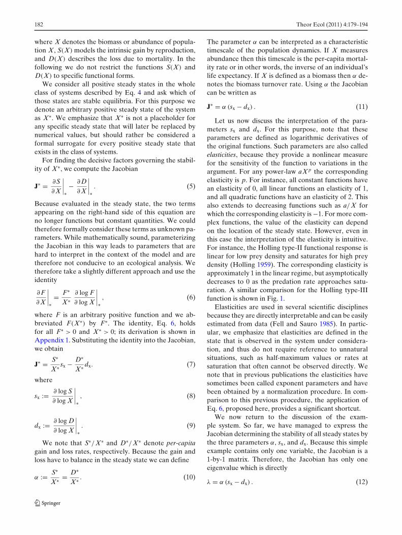
Let us now discuss the interpretation of the para-meters sx and dx. For this purpose, note that theseparameters are defined as logarithmic derivatives ofthe original functions. Such parameters are also calledelasticities, because they provide a nonlinear measurefor the sensitivity of the function to variations in theargument. For any power-law aX p the correspondingelasticity is p. For instance, all constant functions havean elasticity of 0, all linear functions an elasticity of 1,and all quadratic functions have an elasticity of 2. Thisalso extends to decreasing functions such as a/X forwhich the corresponding elasticity is −1. For more com-plex functions, the value of the elasticity can dependon the location of the steady state. However, even inthis case the interpretation of the elasticity is intuitive.For instance, the Holling type-II functional response islinear for low prey density and saturates for high preydensity (Holling 1959). The corresponding elasticity isapproximately 1 in the linear regime, but asymptoticallydecreases to 0 as the predation rate approaches satu-ration. A similar comparison for the Holling type-IIIfunction is shown in Fig. 1.

Elasticities are used in several scientific disciplinesbecause they are directly interpretable and can be easilyestimated from data (Fell and Sauro 1985). In partic-ular, we emphasize that elasticities are defined in thestate that is observed in the system under considera-tion, and thus do not require reference to unnaturalsituations, such as half-maximum values or rates atsaturation that often cannot be observed directly. Wenote that in previous publications the elasticities havesometimes been called exponent parameters and havebeen obtained by a normalization procedure. In com-parison to this previous procedure, the application ofEq. 6, proposed here, provides a significant shortcut.

We now return to the discussion of the exam-ple system. So far, we have managed to express theJacobian determining the stability of all steady states bythe three parameters α, sx, and dx. Because this simpleexample contains only one variable, the Jacobian is a1-by-1 matrix. Therefore, the Jacobian has only oneeigenvalue which is directly

λ = α (sx − dx) . (12)

Theor Ecol (2011) 4:179–194 183

a

b

Fig. 1 Illustration of elasticity. a In the specific example system,a reproduction rate, S(X) of the form of a Holling type-IIIfunctional response, aX2/(k2 + X2), is assumed. This functionstarts out quadratically at low values of the population densityX, but saturates as X increases. b The corresponding elasticity,sx, is close to two near the quadratic regime χ = X∗/k ≈ 0, butapproaches zero as saturation sets in

The steady state under consideration is stable if λ < 0,or equivalently

sx < dx. (13)

In words: In every system of the form of Eq. 4, a givensteady state is stable whenever the elasticity of themortality in the steady state exceeds the elasticity ofreproduction.

A change in stability occurs when the elasticities ofgain and loss become equal,

sx = dx. (14)

If this occurs the eigenvalue of the Jacobian vanishesand the system undergoes a saddle-node bifurcation.

For gaining a deeper understanding of how the gen-eralized analysis relates to conventional models, it isuseful to consider a specific example. We emphasizethat this step is not part of the analysis of the gen-eralized model, but is presented here solely for thepurpose of illustration. One model that immediatelycomes to mind is logistic growth, which can formallybe written as a linear reproduction and quadratic mor-tality. However, based on our discussion above, it isimmediately apparent that linear reproduction must

correspond to sx = 1 and quadratic mortality to dx = 2.Without further analysis we can therefore say thatsteady states found for a single population under logis-tic growth must always be stable regardless of the otherparameters.

A more interesting example is obtained when oneassumes a reproduction rate following a Holling type-III kinetic and linear mortality,

ddt

X = aX2

k2 + X2− b X, (15)

where a is the growth rate at saturation, k is the half-saturation value of growth, and b is the mortality rate.This example system can be investigated by explicitcomputation of steady states and subsequent stabilityand bifurcation analysis. This procedure is shown inmost textbooks on mathematical ecology and is henceomitted here. For the present example the conventionalanalysis reveals that, for high k only a trivial equilib-rium at zero population density exists, so that the pop-ulation becomes extinct deterministically (Fig. 2a). Ask is reduced, a saddle-node bifurcation occurs, whichmarks the onset of a strong Allee effect. In the bifur-cation, a stable nontrivial equilibrium and an unstablesaddle point are created. Beyond the bifurcation a pop-ulation can persist if its initial abundance is above thesaddle point. In this case, the population asymptoticallyapproaches the stable equilibrium. By contrast, a popu-lation which is initially below the saddle point declinesfurther and approaches the trivial (extinct) equilibrium.

For comparing the results from the specific analysisto the generalized model, we compute the elasticitiesthat characterize the steady states found in the specificmodel. Because the mortality rate is assumed to belinear, we know dx = 1. The elasticity of the growthfunction can be found by applying Eq. 6 to the knowngrowth function of the specific model. This yields

sx = 2

1 + χ2(16)

where χ = X∗/k. A detailed derivation of this rela-tionship using a normalization procedure instead ofthe shortcut, Eq. 6, is given in Gross et al. (2004).Equation 16 shows that the elasticity of growth is sx ≈ 2for X∗ � k, but approaches sx = 0 in the limit X∗ � k(Fig. 1).

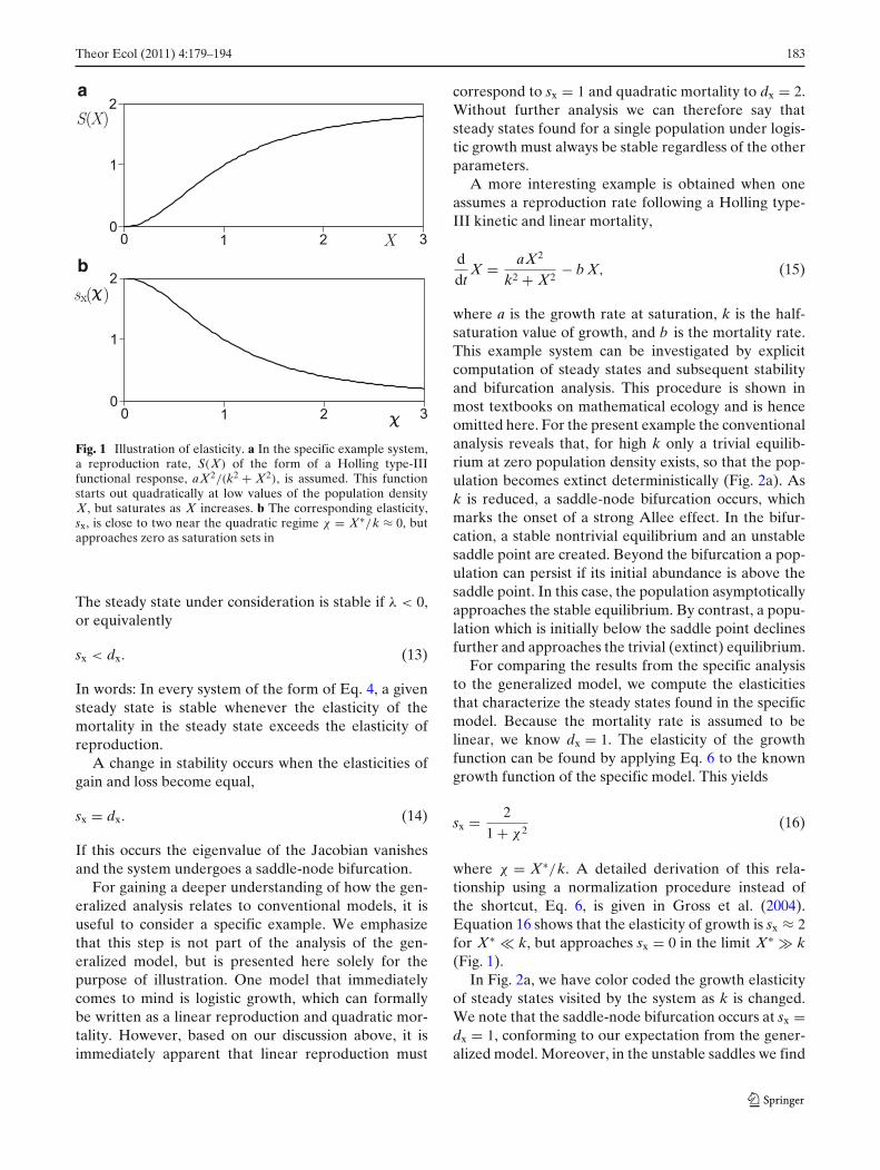
In Fig. 2a, we have color coded the growth elasticityof steady states visited by the system as k is changed.We note that the saddle-node bifurcation occurs at sx =dx = 1, conforming to our expectation from the gener-alized model. Moreover, in the unstable saddles we find

184 Theor Ecol (2011) 4:179–194

ba

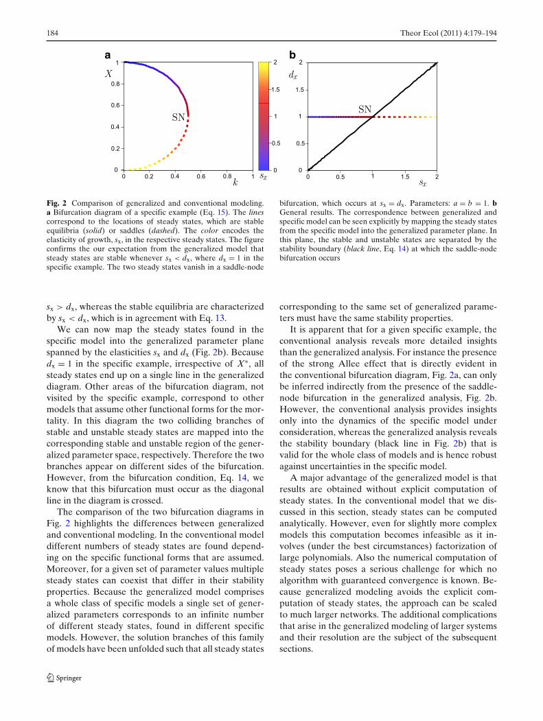
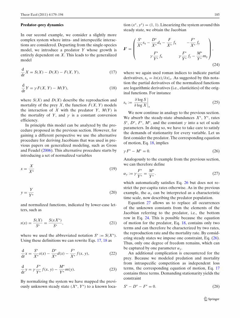
Fig. 2 Comparison of generalized and conventional modeling.a Bifurcation diagram of a specific example (Eq. 15). The linescorrespond to the locations of steady states, which are stableequilibria (solid) or saddles (dashed). The color encodes theelasticity of growth, sx, in the respective steady states. The figureconfirms the our expectation from the generalized model thatsteady states are stable whenever sx < dx, where dx = 1 in thespecific example. The two steady states vanish in a saddle-node

bifurcation, which occurs at sx = dx. Parameters: a = b = 1. bGeneral results. The correspondence between generalized andspecific model can be seen explicitly by mapping the steady statesfrom the specific model into the generalized parameter plane. Inthis plane, the stable and unstable states are separated by thestability boundary (black line, Eq. 14) at which the saddle-nodebifurcation occurs

sx > dx, whereas the stable equilibria are characterizedby sx < dx, which is in agreement with Eq. 13.

We can now map the steady states found in thespecific model into the generalized parameter planespanned by the elasticities sx and dx (Fig. 2b). Becausedx = 1 in the specific example, irrespective of X∗, allsteady states end up on a single line in the generalizeddiagram. Other areas of the bifurcation diagram, notvisited by the specific example, correspond to othermodels that assume other functional forms for the mor-tality. In this diagram the two colliding branches ofstable and unstable steady states are mapped into thecorresponding stable and unstable region of the gener-alized parameter space, respectively. Therefore the twobranches appear on different sides of the bifurcation.However, from the bifurcation condition, Eq. 14, weknow that this bifurcation must occur as the diagonalline in the diagram is crossed.

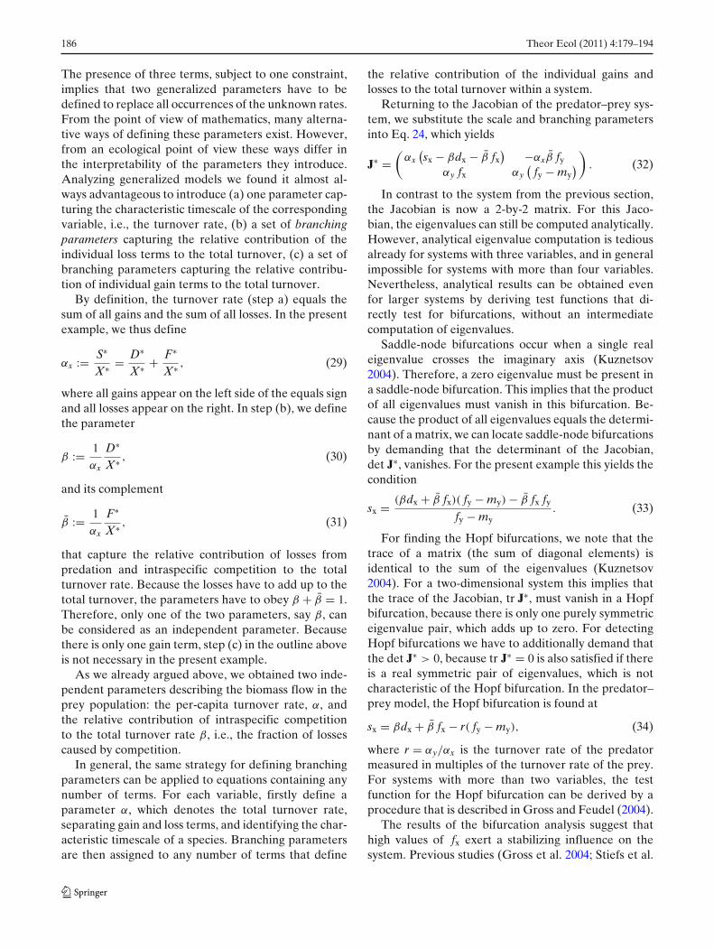
The comparison of the two bifurcation diagrams inFig. 2 highlights the differences between generalizedand conventional modeling. In the conventional modeldifferent numbers of steady states are found depend-ing on the specific functional forms that are assumed.Moreover, for a given set of parameter values multiplesteady states can coexist that differ in their stabilityproperties. Because the generalized model comprisesa whole class of specific models a single set of gener-alized parameters corresponds to an infinite numberof different steady states, found in different specificmodels. However, the solution branches of this familyof models have been unfolded such that all steady states

corresponding to the same set of generalized parame-ters must have the same stability properties.

It is apparent that for a given specific example, theconventional analysis reveals more detailed insightsthan the generalized analysis. For instance the presenceof the strong Allee effect that is directly evident inthe conventional bifurcation diagram, Fig. 2a, can onlybe inferred indirectly from the presence of the saddle-node bifurcation in the generalized analysis, Fig. 2b.However, the conventional analysis provides insightsonly into the dynamics of the specific model underconsideration, whereas the generalized analysis revealsthe stability boundary (black line in Fig. 2b) that isvalid for the whole class of models and is hence robustagainst uncertainties in the specific model.

A major advantage of the generalized model is thatresults are obtained without explicit computation ofsteady states. In the conventional model that we dis-cussed in this section, steady states can be computedanalytically. However, even for slightly more complexmodels this computation becomes infeasible as it in-volves (under the best circumstances) factorization oflarge polynomials. Also the numerical computation ofsteady states poses a serious challenge for which noalgorithm with guaranteed convergence is known. Be-cause generalized modeling avoids the explicit com-putation of steady states, the approach can be scaledto much larger networks. The additional complicationsthat arise in the generalized modeling of larger systemsand their resolution are the subject of the subsequentsections.

Theor Ecol (2011) 4:179–194 185

Predator–prey dynamics

In our second example, we consider a slightly morecomplex system where intra- and interspecific interac-tions are considered. Departing from the single-speciesmodel, we introduce a predator Y whose growth isentirely dependent on X. This leads to the generalizedmodel

ddt

X = S(X) − D(X) − F(X, Y), (17)

ddt

Y = γ F(X, Y) − M(Y), (18)

where S(X) and D(X) describe the reproduction andmortality of the prey X, the function F(X, Y) modelsthe interaction of X with the predator Y, M(Y) isthe mortality of Y, and γ is a constant conversionefficiency.

In principle this model can be analyzed by the pro-cedure proposed in the previous section. However, forgaining a different perspective we use the alternativeprocedure for deriving Jacobians that was used in pre-vious papers on generalized modeling, such as Grossand Feudel (2006). This alternative procedure starts byintroducing a set of normalized variables

x = XX∗ (19)

y = YY∗ (20)

and normalized functions, indicated by lower-case let-ters, such as

s(x) = S(X)

S∗ = S(xX∗)S∗ , (21)

where we used the abbreviated notation S∗ := S(X∗).Using these definitions we can rewrite Eqs. 17, 18 as

ddt

x = S∗

X∗ s(x) − D∗

X∗ d(x) − F∗

X∗ f (x, y), (22)

ddt

y = γF∗

Y∗ f (x, y) − M∗

Y∗ m(y). (23)

By normalizing the system we have mapped the previ-ously unknown steady state (X∗, Y∗) to a known loca-

tion (x∗, y∗) = (1, 1). Linearizing the system around thissteady state, we obtain the Jacobian

J∗ =

⎛

⎜⎜⎜⎝

S∗

X∗ sx − D∗

X∗ dx − FX∗ fx − F∗

X∗ fy

γF∗

Y∗ fx γF∗

Y∗ fy − M∗

Y∗ my

⎞

⎟⎟⎟⎠

,

(24)

where we again used roman indices to indicate partialderivatives, sx = ∂s(x)/∂x|∗. As suggested by this nota-tion the partial derivatives of the normalized functionsare logarithmic derivatives (i.e., elasticities) of the orig-inal functions. For instance

sx := ∂ log S∂ log X

∣∣∣∣∗

(25)

We now continue in analogy to the previous section.We absorb the steady-state abundances X∗, Y∗, ratesS∗, D∗, F∗, M∗, and the constant γ into a set of scaleparameters. In doing so, we have to take care to satisfythe demands of stationarity for every variable. Let usfirst consider the predator. The corresponding equationof motion, Eq. 18, implies

γ F∗ − M∗ = 0. (26)

Analogously to the example from the previous section,we can therefore define

αy := γF∗

Y∗ = M∗

Y∗ . (27)

which automatically satisfies Eq. 26 but does not re-strict the per-capita rates otherwise. As in the previousexample, the αy can be interpreted as a characteristictime scale, now describing the predator population.

Equation 27 allows us to replace all occurrencesof the unknown constants from the elements of theJacobian referring to the predator, i.e., the bottomrow in Eq. 24. This is possible because the equationof motion for the predator, Eq. 18, contains only twoterms and can therefore be characterized by two rates,the reproduction rate and the mortality rate. By consid-ering steady states we impose one constraint, Eq. (26).Thus, only one degree of freedom remains, which canbe captured by one parameter αy.

An additional complication is encountered for theprey. Because we modeled predation and mortalityfrom intraspecific competition as independent lossterms, the corresponding equation of motion, Eq. 17contains three terms. Demanding stationarity yields theconstraint

S∗ − D∗ − F∗ = 0. (28)

186 Theor Ecol (2011) 4:179–194

The presence of three terms, subject to one constraint,implies that two generalized parameters have to bedefined to replace all occurrences of the unknown rates.From the point of view of mathematics, many alterna-tive ways of defining these parameters exist. However,from an ecological point of view these ways differ inthe interpretability of the parameters they introduce.Analyzing generalized models we found it almost al-ways advantageous to introduce (a) one parameter cap-turing the characteristic timescale of the correspondingvariable, i.e., the turnover rate, (b) a set of branchingparameters capturing the relative contribution of theindividual loss terms to the total turnover, (c) a set ofbranching parameters capturing the relative contribu-tion of individual gain terms to the total turnover.

By definition, the turnover rate (step a) equals thesum of all gains and the sum of all losses. In the presentexample, we thus define

αx := S∗

X∗ = D∗

X∗ + F∗

X∗ , (29)

where all gains appear on the left side of the equals signand all losses appear on the right. In step (b), we definethe parameter

β := 1

αx

D∗

X∗ , (30)

and its complement

β̄ := 1

αx

F∗

X∗ , (31)

that capture the relative contribution of losses frompredation and intraspecific competition to the totalturnover rate. Because the losses have to add up to thetotal turnover, the parameters have to obey β + β̄ = 1.Therefore, only one of the two parameters, say β, canbe considered as an independent parameter. Becausethere is only one gain term, step (c) in the outline aboveis not necessary in the present example.

As we already argued above, we obtained two inde-pendent parameters describing the biomass flow in theprey population: the per-capita turnover rate, α, andthe relative contribution of intraspecific competitionto the total turnover rate β, i.e., the fraction of lossescaused by competition.

In general, the same strategy for defining branchingparameters can be applied to equations containing anynumber of terms. For each variable, firstly define aparameter α, which denotes the total turnover rate,separating gain and loss terms, and identifying the char-acteristic timescale of a species. Branching parametersare then assigned to any number of terms that define

the relative contribution of the individual gains andlosses to the total turnover within a system.

Returning to the Jacobian of the predator–prey sys-tem, we substitute the scale and branching parametersinto Eq. 24, which yields

J∗ =(

αx(

sx − βdx − β̄ fx) −αxβ̄ fy

αy fx αy(

fy − my)

)

. (32)

In contrast to the system from the previous section,the Jacobian is now a 2-by-2 matrix. For this Jaco-bian, the eigenvalues can still be computed analytically.However, analytical eigenvalue computation is tediousalready for systems with three variables, and in generalimpossible for systems with more than four variables.Nevertheless, analytical results can be obtained evenfor larger systems by deriving test functions that di-rectly test for bifurcations, without an intermediatecomputation of eigenvalues.

Saddle-node bifurcations occur when a single realeigenvalue crosses the imaginary axis (Kuznetsov2004). Therefore, a zero eigenvalue must be present ina saddle-node bifurcation. This implies that the productof all eigenvalues must vanish in this bifurcation. Be-cause the product of all eigenvalues equals the determi-nant of a matrix, we can locate saddle-node bifurcationsby demanding that the determinant of the Jacobian,det J∗, vanishes. For the present example this yields thecondition

sx = (βdx + β̄ fx)( fy − my) − β̄ fx fy

fy − my. (33)

For finding the Hopf bifurcations, we note that thetrace of a matrix (the sum of diagonal elements) isidentical to the sum of the eigenvalues (Kuznetsov2004). For a two-dimensional system this implies thatthe trace of the Jacobian, tr J∗, must vanish in a Hopfbifurcation, because there is only one purely symmetriceigenvalue pair, which adds up to zero. For detectingHopf bifurcations we have to additionally demand thatthe det J∗ > 0, because tr J∗ = 0 is also satisfied if thereis a real symmetric pair of eigenvalues, which is notcharacteristic of the Hopf bifurcation. In the predator–prey model, the Hopf bifurcation is found at

sx = βdx + β̄ fx − r( fy − my), (34)

where r = αy/αx is the turnover rate of the predatormeasured in multiples of the turnover rate of the prey.For systems with more than two variables, the testfunction for the Hopf bifurcation can be derived by aprocedure that is described in Gross and Feudel (2004).

The results of the bifurcation analysis suggest thathigh values of fx exert a stabilizing influence on thesystem. Previous studies (Gross et al. 2004; Stiefs et al.

Theor Ecol (2011) 4:179–194 187

2010) showed that this parameter is relevant for en-richment scenarios. In many previously proposed mod-els, predator saturation increases when resources areadded, leading to a decrease of fx and therefore toinstability. Identification of fx as a crucial parameterfor stability in the generalized model enables us to askwhat functional responses would lead to an intermedi-ate stabilizing effect of enrichment that is sometimesobserved in nature. The discussion in Gross et al. (2004)showed that reasonable functional responses can befound that exhibit such an intermediate stabilization,but are very hard to distinguish from, say Holling type-II kinetics, if they were encountered in nature.

To illustrate the differences between generalized andconventional modeling, we again compare the general-ized model with a specific example. For this purposewe focus on the Rosenzweig–MacArthur model. In thismodel, the prey exhibits logistic growth in absence ofthe predator, the predator–prey interaction is modeledby a Holling type-II functional response, and the mor-tality of the predator is assumed to be density indepen-dent. This leads to

ddt

X = rX(

1 − Xk

)

− aXYb + X

,

ddt

Y = γaXY

b + X− mY, (35)

where r is the intrinsic growth rate of X, k is the carry-ing capacity of X, a is the predation rate at saturation,b is the half-saturation value of the predation rate,γ is the biomass conversion efficiency, and m is themortality rate of Y.

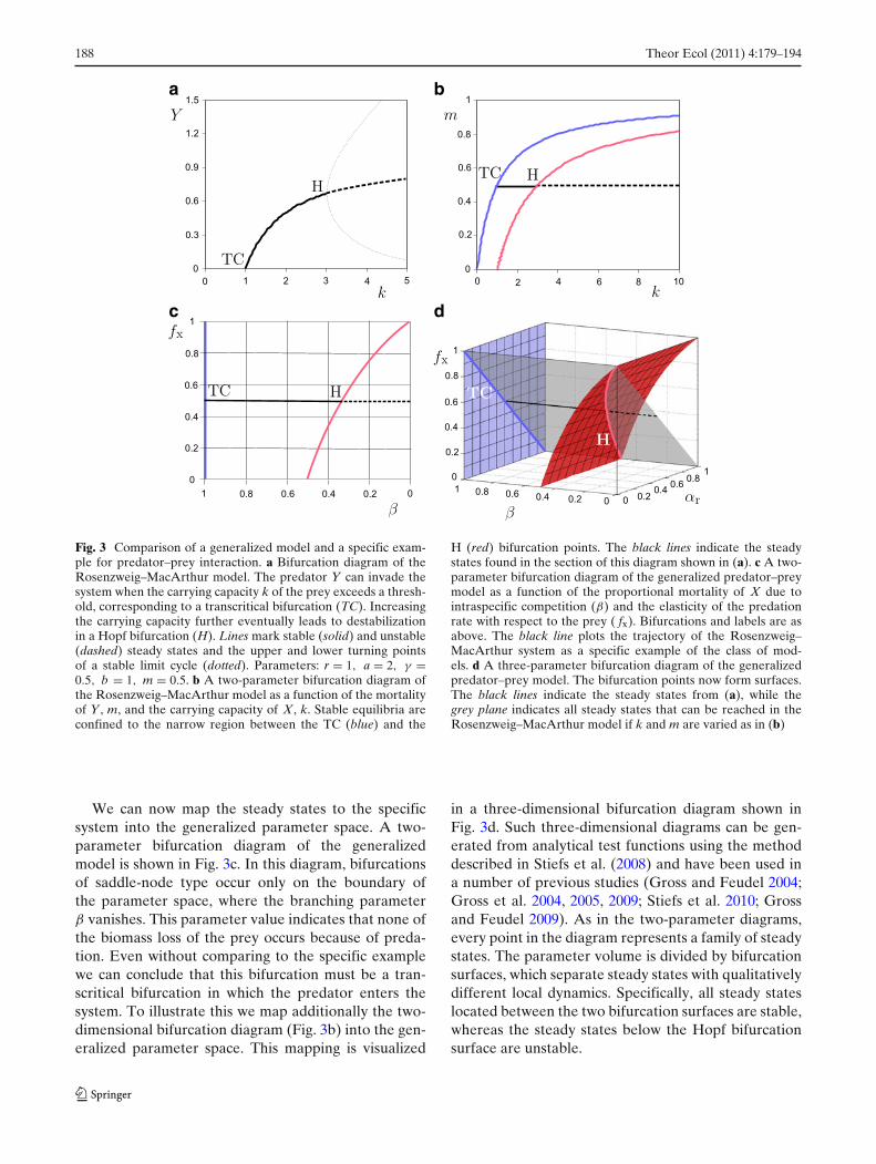
The results of a conventional bifurcation analysis areshown in Fig. 3a. If the carrying capacity k is too smallthen the predator population cannot invade the system.As the carrying capacity is increased a transcritical bi-furcation occurs in which a stable equilibrium appears,such that the predator–prey system can reside in sta-tionarity. If the carrying capacity is increased further,a supercritical Hopf bifurcation occurs, in which theequilibrium is destabilized. Subsequently, the systemresides on a stable limit cycle, which emerges from theHopf bifurcation. On this cycle, pronounced predator–prey oscillations can be observed, which become largeras the carrying capacity is further increased.

One can imagine that if an additional parameteris changed then critical values of the carrying capac-ity at which the bifurcations occur change as well.This can be visualized in two-parameter bifurcationdiagrams, which we have already used for the gen-eralized model in Fig. 2b. In such diagrams, Hopfand saddle-node bifurcation points form lines in the

two-dimensional parameter space. For the specific ex-ample of the Rosenzweig–MacArthur system, a two-parameter bifurcation diagram is shown in Fig. 3b. Thisdiagram illustrates that increasing the mortality rate mof the predator, shifts both the transcritical bifurcationpoint and the Hopf bifurcation point to higher values ofthe carrying capacity.

For comparing the specific example to the gener-alized model, we compute the generalized parametersthat are observed in the steady states of the specificmodel. Above, we have already noted that logisticgrowth can be understood as a combination of linear re-production and quadratic mortality, which correspondsto sx = 1 and dx = 2. Furthermore, the assumptions ofdensity independent mortality and linear dependenceof the predation rate on the predator imply my =fy = 1. The elasticity fx of the predation rate withrespect to prey was derived in Gross et al. (2004) andis

fx = 1

1 + χ, (36)

where χ = X∗/b . Accordingly, fx = 1 in the limit ofvanishing prey density and fx = 0 in the limit of infiniteprey. Note that in the Rosenzweig–MacArthur model,the predator population tightly controls the prey pop-ulation. Once the predator can invade, any furtherincrease in carrying capacity only increases the station-ary population of the predator, while the stationarypopulation size of the prey remains invariant.

Apart from the parameters β and fx, shown inFig. 3c, the only other parameter that is not fixed toa specific value is the relative turnover of the predatorr = αy/αx. This parameter cannot affect the transcrit-ical bifurcation, because turnover rates by construc-tion cannot appear in test functions of transcritical orsaddle-node bifurcations. By contrast, turnover ratesin general affect Hopf bifurcations. However, in thepresent example the dependence of the Hopf bifur-cation test function, Eq. 34 on r disappears if densityindependent mortality and linear dependence of thepredation rate on the predator population are assumed.Therefore, the parameter has no influence on the bi-furcation surfaces. We note that this is a special prop-erty of the Rosenzweig–MacArthur system and not ageneric feature of the larger class of systems describedby the generalized model. As argued in van Voorn et al.(2007) and Gross and Feudel (2009) one can expectthat typically mortality is slightly super-linear becauseof overcrowding, diseases and other limiting resources,whereas predation may be sublinear due to predatorinterference. In this case, large values of r can have astabilizing effect.

188 Theor Ecol (2011) 4:179–194

d

b

c

a

Fig. 3 Comparison of a generalized model and a specific exam-ple for predator–prey interaction. a Bifurcation diagram of theRosenzweig–MacArthur model. The predator Y can invade thesystem when the carrying capacity k of the prey exceeds a thresh-old, corresponding to a transcritical bifurcation (TC). Increasingthe carrying capacity further eventually leads to destabilizationin a Hopf bifurcation (H). Lines mark stable (solid) and unstable(dashed) steady states and the upper and lower turning pointsof a stable limit cycle (dotted). Parameters: r = 1, a = 2, γ =0.5, b = 1, m = 0.5. b A two-parameter bifurcation diagram ofthe Rosenzweig–MacArthur model as a function of the mortalityof Y, m, and the carrying capacity of X, k. Stable equilibria areconfined to the narrow region between the TC (blue) and the

H (red) bifurcation points. The black lines indicate the steadystates found in the section of this diagram shown in (a). c A two-parameter bifurcation diagram of the generalized predator–preymodel as a function of the proportional mortality of X due tointraspecific competition (β) and the elasticity of the predationrate with respect to the prey ( fx). Bifurcations and labels are asabove. The black line plots the trajectory of the Rosenzweig–MacArthur system as a specific example of the class of mod-els. d A three-parameter bifurcation diagram of the generalizedpredator–prey model. The bifurcation points now form surfaces.The black lines indicate the steady states from (a), while thegrey plane indicates all steady states that can be reached in theRosenzweig–MacArthur model if k and m are varied as in (b)

We can now map the steady states to the specificsystem into the generalized parameter space. A two-parameter bifurcation diagram of the generalizedmodel is shown in Fig. 3c. In this diagram, bifurcationsof saddle-node type occur only on the boundary ofthe parameter space, where the branching parameterβ vanishes. This parameter value indicates that none ofthe biomass loss of the prey occurs because of preda-tion. Even without comparing to the specific examplewe can conclude that this bifurcation must be a tran-scritical bifurcation in which the predator enters thesystem. To illustrate this we map additionally the two-dimensional bifurcation diagram (Fig. 3b) into the gen-eralized parameter space. This mapping is visualized

in a three-dimensional bifurcation diagram shown inFig. 3d. Such three-dimensional diagrams can be gen-erated from analytical test functions using the methoddescribed in Stiefs et al. (2008) and have been used ina number of previous studies (Gross and Feudel 2004;Gross et al. 2004, 2005, 2009; Stiefs et al. 2010; Grossand Feudel 2009). As in the two-parameter diagrams,every point in the diagram represents a family of steadystates. The parameter volume is divided by bifurcationsurfaces, which separate steady states with qualitativelydifferent local dynamics. Specifically, all steady stateslocated between the two bifurcation surfaces are stable,whereas the steady states below the Hopf bifurcationsurface are unstable.

Theor Ecol (2011) 4:179–194 189

In the present example, we were able to show allrelevant parameters in a single three-parameter bifur-cation diagram. Let us remark that this is in generalnot possible as a larger number of parameters is oftennecessary to capture the dynamics of a system at the de-sired degree of generality. Even if a generalized modelcontains only five parameters, the three-dimensionalslice that can be visualized in a single three-parameterdiagram is relatively small when compared with thefive-dimensional space. Nevertheless, plotting three-parameter bifurcation diagrams can be very valuablebecause a three-dimensional diagram is often sufficientto locate bifurcations of higher codimension. Such bi-furcations are formed at the point in parameter spacewhere different bifurcation surfaces meet or intersect.The presence of such bifurcations can reveal additionalinsights into global properties of the dynamics. Forinstance in Gross et al. (2005) the presence of a certainbifurcation of higher codimension in generalized mod-els was used to show that chaotic dynamics genericallyexist in long food chains. An extensive discussion ofbifurcations of higher codimension and their dynami-cal implications is presented in Kuznetsov (2004). Forobtaining a general overview of the dynamics of largersystems containing hundreds or thousands of parame-ters, bifurcation diagrams are not suitable. However,these systems can be analyzed by statistical samplingtechniques described in the following section.

Intraguild predation

As the final example in the present paper, we considerthe effect of omnivory on a small food web. Omnivoryis defined by an organism’s ability to consume prey thatinhabit multiple trophic levels. It has been the subjectof much recent interest because it is notable for its per-vasiveness within well-studied ecosystems (Polis 1991),as well as its relatively complex dynamics (McCann andHastings 1997; Kuijper et al. 2003; Tanabe and Namba2008).

Omnivory has been historically viewed as a para-doxical interaction. Initially, the presence of om-nivory was thought to be entirely destabilizing, and,as a consequence, rarely observed in nature (Pimmand Lawton 1978). However, further explorations ofecological networks have reported omnivory to be acommon architectural component within larger foodwebs (Bascompte et al. 2005; Stouffer and Bascompte2010). Furthermore, theoretical investigations have re-vealed parameter regions that lead to both stabilizingand destabilizing dynamics in simple models (Holt andPolis 1997; McCann and Hastings 1997; Kuijper et al.

2003; Tanabe and Namba 2008; Namba et al. 2008;Verdy and Amarasekare 2010). These theoretical ar-guments are limited by the fact that such models areeither constrained to specific functional forms or reportdynamics across parameter ranges that may not bebiologically significant. A generalization of the entireclass of simple omnivory models is poised to elucidateunder which conditions stable or unstable dynamics arebound to occur, regardless of the functional relation-ships among or between species in the model.

A specific case of omnivory is intraguild predation(IGP), which in its simplest incarnation appears in athree-species system containing a consumer and re-source pair (as in the prior example), and an omnivorethat predates upon both the consumer and resource.Traditional analyses of IGP models reached the follow-ing: (1) the coexistence of all species in the system iscontingent on the greater competitive abilities of Y,relative to the omnivore Z , to consume the sharedresource (Holt and Polis 1997; McCann and Hastings1997); (2) enrichment destabilizes the system (Holt andPolis 1997; Diehl and Feissel 2001); (3) if the gain ofthe omnivore by predation on the consumer exceedsthe negative competitive effects of the consumer, thenthe consumer facilitates a larger population of the om-nivore than can be maintained in its absence (Diehl andFeissel 2001).

In the present paper, we consider the generalizedmodel

ddt

X = S(X) − D(X) − F(X, Y) − G(X, Y, Z )

ddt

Y = γ F(X, Y) − H(X, Y, Z ) − M(Y)

ddt

Z = K(X, Y, Z ) − M(Z ). (37)

In addition to the terms already presented in thepredator–prey model from “Predator–prey dynamics”,we included the functions G and H, which denote theloss of the resource and consumer from predation bythe omnivore and the function K denoting the gain ofthe omnivore that arises from this predation. Note thatwe modeled the two different predatory losses of X asseparate terms G and H because these losses can beassumed to arise independently of each other. By con-trast the gain of the omnivore derives from predationon two different prey species and is modeled as a singleterm K because finite handling time, saturation effects,and possibly active prey-switching behavior prevent thepredator from feeding on both sources independentlyof each other.

190 Theor Ecol (2011) 4:179–194

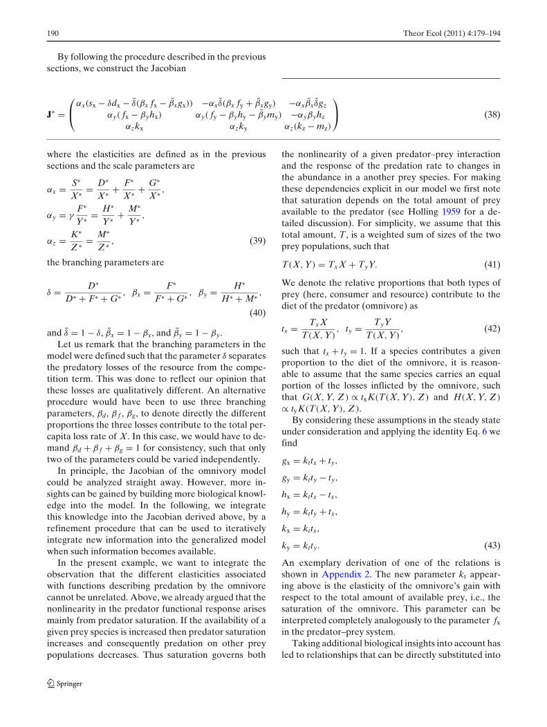
By following the procedure described in the previoussections, we construct the Jacobian

J∗ =⎛

⎝

αx(sx − δdx − δ̄(βx fx − β̄xgx)) −αxδ̄(βx fy + β̄xgy) −αxβ̄xδ̄gz

αy( fx − βyhx) αy( fy − βyhy − β̄ymy) −αyβyhz

αzkx αzky αz(kz − mz)

⎞

⎠ (38)

where the elasticities are defined as in the previoussections and the scale parameters are

αx = S∗

X∗ = D∗

X∗ + F∗

X∗ + G∗

X∗ ,

αy = γF∗

Y∗ = H∗

Y∗ + M∗

Y∗ ,

αz = K∗

Z ∗ = M∗

Z ∗ , (39)

the branching parameters are

δ = D∗

D∗ + F∗ + G∗ , βx = F∗

F∗ + G∗ , βy = H∗

H∗ + M∗ ,

(40)

and δ̄ = 1 − δ, β̄x = 1 − βx, and β̄y = 1 − βy.Let us remark that the branching parameters in the

model were defined such that the parameter δ separatesthe predatory losses of the resource from the compe-tition term. This was done to reflect our opinion thatthese losses are qualitatively different. An alternativeprocedure would have been to use three branchingparameters, βd, β f , βg, to denote directly the differentproportions the three losses contribute to the total per-capita loss rate of X. In this case, we would have to de-mand βd + β f + βg = 1 for consistency, such that onlytwo of the parameters could be varied independently.

In principle, the Jacobian of the omnivory modelcould be analyzed straight away. However, more in-sights can be gained by building more biological knowl-edge into the model. In the following, we integratethis knowledge into the Jacobian derived above, by arefinement procedure that can be used to iterativelyintegrate new information into the generalized modelwhen such information becomes available.

In the present example, we want to integrate theobservation that the different elasticities associatedwith functions describing predation by the omnivorecannot be unrelated. Above, we already argued that thenonlinearity in the predator functional response arisesmainly from predator saturation. If the availability of agiven prey species is increased then predator saturationincreases and consequently predation on other preypopulations decreases. Thus saturation governs both

the nonlinearity of a given predator–prey interactionand the response of the predation rate to changes inthe abundance in a another prey species. For makingthese dependencies explicit in our model we first notethat saturation depends on the total amount of preyavailable to the predator (see Holling 1959 for a de-tailed discussion). For simplicity, we assume that thistotal amount, T, is a weighted sum of sizes of the twoprey populations, such that

T(X, Y) = Tx X + TyY. (41)

We denote the relative proportions that both types ofprey (here, consumer and resource) contribute to thediet of the predator (omnivore) as

tx = Tx XT(X, Y)

, ty = TyYT(X, Y)

, (42)

such that tx + ty = 1. If a species contributes a givenproportion to the diet of the omnivore, it is reason-able to assume that the same species carries an equalportion of the losses inflicted by the omnivore, suchthat G(X, Y, Z ) ∝ tx K(T(X, Y), Z ) and H(X, Y, Z )

∝ ty K(T(X, Y), Z ).By considering these assumptions in the steady state

under consideration and applying the identity Eq. 6 wefind

gx = kttx + ty,

gy = ktty − ty,

hx = kttx − tx,

hy = ktty + tx,

kx = kttx,

ky = ktty. (43)

An exemplary derivation of one of the relations isshown in Appendix 2. The new parameter kt appear-ing above is the elasticity of the omnivore’s gain withrespect to the total amount of available prey, i.e., thesaturation of the omnivore. This parameter can beinterpreted completely analogously to the parameter fx

in the predator–prey system.Taking additional biological insights into account has

led to relationships that can be directly substituted into

Theor Ecol (2011) 4:179–194 191

the previously derived Jacobian. Doing so removes sixparameters from the generalized model at the cost ofintroducing two new ones. The substitution makes themodel less general and more specific, allowing us toextract more conclusions on a narrower range of mod-els. By this procedure new insights on a given systemcan be integrated iteratively without re-engineering themodel from scratch. We believe that such refinementswill be valuable for future food web models possiblycontaining hundreds of species.

Let us remark that iterative refinement is not con-tingent on the availability of a specific, i.e., non-general, equation. Instead of the specific relationshipin Eq. 41, we could have also used the general rela-tionship T(X, Y) = Cx(X) + Cy(Y), where Cx and Cy

are general functions. Even substituting this generalrelationship into the model leads to a reduction of pa-rameters of the model. Furthermore, the functions Cx

and Cy can be used to introduce active prey switching.This has been done for instance in the food web modelsproposed in Gross and Feudel (2006) and Gross et al.(2009).

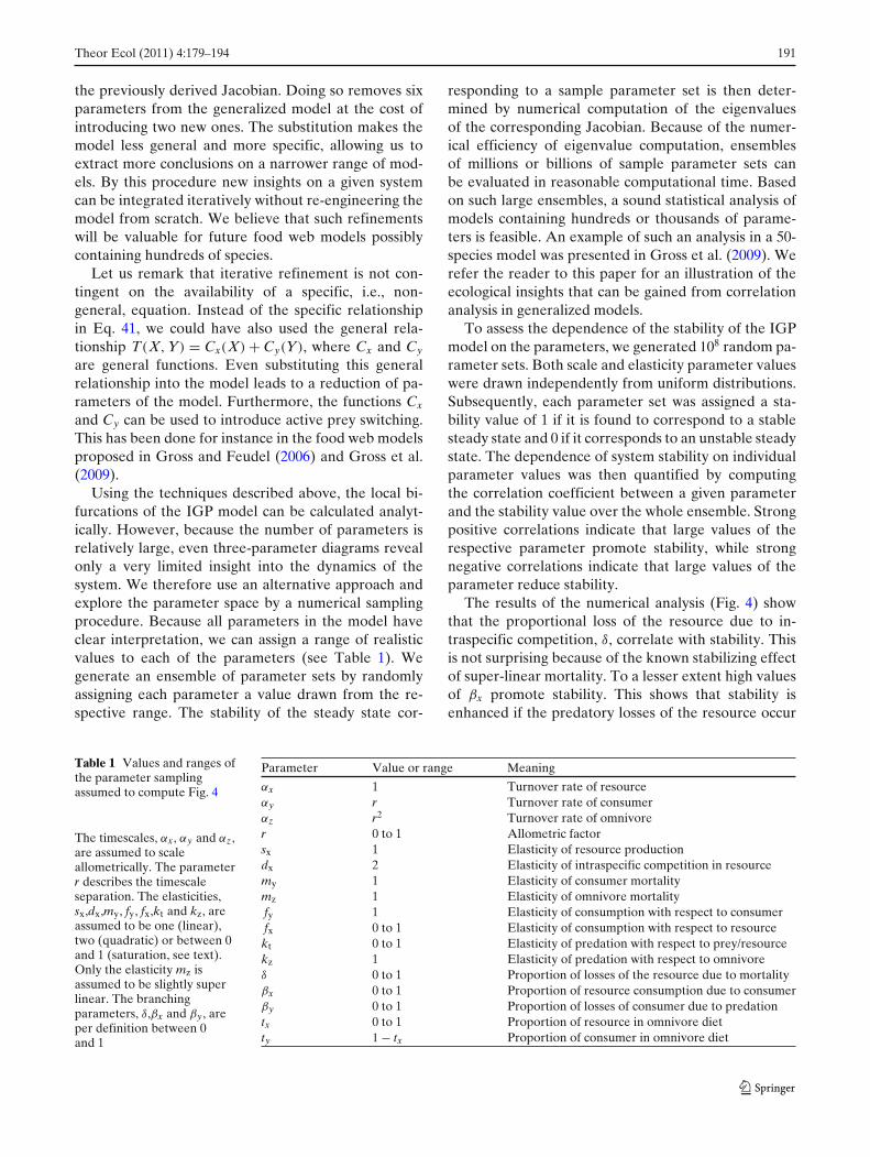
Using the techniques described above, the local bi-furcations of the IGP model can be calculated analyt-ically. However, because the number of parameters isrelatively large, even three-parameter diagrams revealonly a very limited insight into the dynamics of thesystem. We therefore use an alternative approach andexplore the parameter space by a numerical samplingprocedure. Because all parameters in the model haveclear interpretation, we can assign a range of realisticvalues to each of the parameters (see Table 1). Wegenerate an ensemble of parameter sets by randomlyassigning each parameter a value drawn from the re-spective range. The stability of the steady state cor-

responding to a sample parameter set is then deter-mined by numerical computation of the eigenvaluesof the corresponding Jacobian. Because of the numer-ical efficiency of eigenvalue computation, ensemblesof millions or billions of sample parameter sets canbe evaluated in reasonable computational time. Basedon such large ensembles, a sound statistical analysis ofmodels containing hundreds or thousands of parame-ters is feasible. An example of such an analysis in a 50-species model was presented in Gross et al. (2009). Werefer the reader to this paper for an illustration of theecological insights that can be gained from correlationanalysis in generalized models.

To assess the dependence of the stability of the IGPmodel on the parameters, we generated 108 random pa-rameter sets. Both scale and elasticity parameter valueswere drawn independently from uniform distributions.Subsequently, each parameter set was assigned a sta-bility value of 1 if it is found to correspond to a stablesteady state and 0 if it corresponds to an unstable steadystate. The dependence of system stability on individualparameter values was then quantified by computingthe correlation coefficient between a given parameterand the stability value over the whole ensemble. Strongpositive correlations indicate that large values of therespective parameter promote stability, while strongnegative correlations indicate that large values of theparameter reduce stability.

The results of the numerical analysis (Fig. 4) showthat the proportional loss of the resource due to in-traspecific competition, δ, correlate with stability. Thisis not surprising because of the known stabilizing effectof super-linear mortality. To a lesser extent high valuesof βx promote stability. This shows that stability isenhanced if the predatory losses of the resource occur

Table 1 Values and ranges ofthe parameter samplingassumed to compute Fig. 4

The timescales, αx, αy and αz,are assumed to scaleallometrically. The parameterr describes the timescaleseparation. The elasticities,sx,dx,my, fy, fx,kt and kz, areassumed to be one (linear),two (quadratic) or between 0and 1 (saturation, see text).Only the elasticity mz isassumed to be slightly superlinear. The branchingparameters, δ,βx and βy, areper definition between 0and 1

Parameter Value or range Meaning

αx 1 Turnover rate of resourceαy r Turnover rate of consumerαz r2 Turnover rate of omnivorer 0 to 1 Allometric factorsx 1 Elasticity of resource productiondx 2 Elasticity of intraspecific competition in resourcemy 1 Elasticity of consumer mortalitymz 1 Elasticity of omnivore mortalityfy 1 Elasticity of consumption with respect to consumerfx 0 to 1 Elasticity of consumption with respect to resourcekt 0 to 1 Elasticity of predation with respect to prey/resourcekz 1 Elasticity of predation with respect to omnivoreδ 0 to 1 Proportion of losses of the resource due to mortalityβx 0 to 1 Proportion of resource consumption due to consumerβy 0 to 1 Proportion of losses of consumer due to predationtx 0 to 1 Proportion of resource in omnivore dietty 1 − tx Proportion of consumer in omnivore diet

192 Theor Ecol (2011) 4:179–194

Fig. 4 The dependence of the stability of the generalized IGPmodel on the parameters: r, βx, δ, fx, tx, kt and βy. Depen-dencies were quantified by calculating the correlation coefficientsbetween a given parameter and system stability. 108 parameterssets were assigned randomly from uniform distributions overspecified ranges. Error bars are too small to be visible. Strongpositive correlations indicate that large values of the specificparameter promote stability, while strong negative correlationsindicate that large values of the specific parameter promoteinstability. The parameters δ, and to a lesser extent βx, corre-sponding to high intraspecific competition of X and a strongtrophic interaction between X and Y, stabilize the generalizedIGP model. High values of βy, strong extrinsic mortality of Y, isassociated with destabilizing effects. The interpretation of para-meters follows the lines explained in Section Density-dependentgrowth of a single species. Additional information is provided inTable 1

mainly because of predation by the consumer. This isconsistent with observation 1 stated in the introduc-tion of this section that stability is contingent on thegreater competitive ability of the consumer. Further-more, Fig. 4 shows a stabilizing effect of kt and fx,which denote the elasticity of functional responses ofthe omnivore and the consumer respectively. Alreadyin the previous section we linked such elasticities to en-richment. In enrichment scenarios using common func-tional forms these parameters tend to decrease lead-ing to instability, which explains observation 2 statedabove. We remark, however, that moderate enrichmentmay have a stabilizing effect if alternative functionalforms, such as the one proposed in Gross et al. (2004)are used. The third observation, stated above, is hard toinvestigate in the generalized model because it refers toabundances in the steady state, which are not directlyaccessible in the generalized analysis. However, in ad-dition to previous findings the generalized analysis re-veals that the fraction of losses of the consumer causedby the omnivore, βy, is strongly negatively correlatedwith stability. This indicates that scenarios in which the

omnivore benefits from the presence of the consumerare likely to be unstable.

We remark that the precise results of the sam-pling analysis shown here are not independent of thespecific ranges and distributions that are used for gen-erating the ensemble. Although the error bars of thestatistical analysis rapidly become very small, minordifferences between correlation coefficients should notbe over-interpreted. Nevertheless, the stability correla-tion analysis is a powerful tool that can very quicklyconvey an impression of the stabilizing and destabi-lizing factors in large networks. Ideally, this analysisshould be followed up by more refined statistical ex-ploration of the ensemble. More detailed insights in thebehavior of the system can be gained for instance byplotting histograms of the proportion of stable statesthat are found if one parameter is set to a specific value,while all others are varied randomly. Such histogramshave for instance been used in Steuer et al. (2006),Steuer et al. (2007), Gross et al. (2009) and Zumsandeand Gross (2010). Because these more detailed analysesclearly exceed the scope of the present paper, we post-pone further analysis of the IGP model to a separatepublication.

Conclusions

In the present paper, we have illustrated the funda-mental ideas or procedures of generalized modelingand extended the approach of generalized modeling.Generalized models can reveal conditions for the stabil-ity of steady states in large classes of systems, identifythe bifurcations in which stability is lost, and providesome insights into the global dynamics of the system.They can be seen as an intermediate approach thathas many advantages of conventional equation-basedmodels, while coming close to the efficiency of randommatrix models. This efficiency, both in terms of manuallabor and CPU time, highlights generalized modelingas a promising approach for detailed analysis of largeecological systems. Although we have restricted thepresentation to models with up to three variables, thesesimple examples already contain all of the complexitiesthat are encountered in larger systems, such as the 50-species model studied in Gross et al. (2009).

The presentation of generalized modeling in thepresent paper differed significantly from previous pub-lications. The differences arise in part from the strongerfocus on fundamental concepts and modeling strategiesand in part from a newly proposed shortcut that facili-tates the formulation of generalized models

Theor Ecol (2011) 4:179–194 193

Throughout this paper, we have contrasted severalgeneralized models with conventional counterparts.We emphasize that this was done purely for illus-tration of the results of generalized modeling. Gen-eralized modeling should by no means be regardedas an alternative modeling approach replacing con-ventional models. Note that generalized modeling ismainly useful in systems for which little information isavailable, whereas in well-known systems many moreinsights may be extractable by conventional models.We point out that the iterative refinement procedureproposed here, allows a researcher to start out with ageneralized model and then successively integrate newinformation as it becomes available until eventually aconventional model is obtained. Generalized modelingis ideally applied if one asks how and under which con-ditions a given dynamical phenomenon, such as stablecoexistence, oscillations or chaos, is possible. Becauseof its efficiency and generality, generalized modelingcan then be used to explore a large range of modelstructures for evidence pointing to the phenomenon un-der consideration. Thereby, promising specific modelsystems can be identified which can subsequently beanalyzed in more detail by conventional model analysis.

Open Access This article is distributed under the terms of theCreative Commons Attribution Noncommercial License whichpermits any noncommercial use, distribution, and reproductionin any medium, provided the original author(s) and source arecredited.

Appendix 1

The formulation of elasticity parameters is contingenton the relationship

∂ F∂ X

∣∣∣∣∗

= F∗

X∗∂ log F∂ log X

∣∣∣∣∗

(44)

where F represents some function of X. For provingthis relationship, we consider the right-hand side andmultiply it by 1 = ∂ F/∂ F

F∗

X∗∂ log F

∂ F∂ F

∂ log X

∣∣∣∣∗

, (45)

where (∂ log F/∂ F)∗ simplifies to 1/F∗. This results in

∂ F∂ X

∣∣∣∣∗

= 1

X∗∂ F

∂ log X

∣∣∣∣∗

. (46)

In the previous steps, we replaced log F in the numera-tor of the derivative. To replace log X in the numeratorwe proceed analogously

∂ F∂ X

∣∣∣∣∗

= 1

X∗∂ X

∂ log X∂ F∂ X

∣∣∣∣∗

, (47)

We now consider the second factor of the right-handside. To evaluate the partial derivative we define X =eu and write

∂ X∂ log X

∣∣∣∣∗

= ∂eu

∂ log eu

∣∣∣∣∗

= ∂eu

∂u

∣∣∣∣∗

= eu∣∣∗ = X∗. (48)

substituting back into Eq. 47 we obtain

∂ F∂ X∗

∣∣∣∣∗

= 1

X∗ X∗ ∂ F∂ X

∣∣∣∣∗

= ∂ F∂ X

∣∣∣∣∗

. (49)

which proves Eq. 44.

Appendix 2

Starting from

G(T(X, Y), Z ) = εgTX XT(X, Y)

K(T(X, Y), Z ) (50)

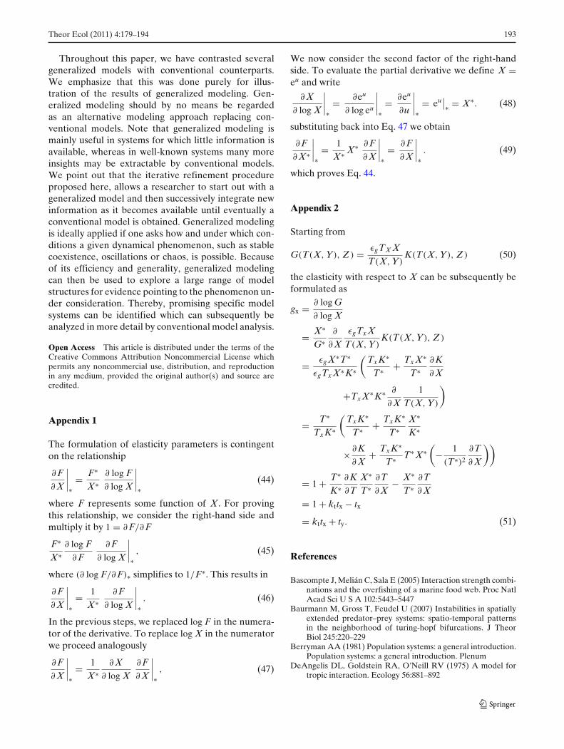
the elasticity with respect to X can be subsequently beformulated as

gx = ∂ log G∂ log X

= X∗

G∗∂

∂ XεgTx X

T(X, Y)K(T(X, Y), Z )

= εg X∗T∗

εgTx X∗K∗

(Tx K∗

T∗ + Tx X∗

T∗∂K∂ X

+Tx X∗K∗ ∂

∂ X1

T(X, Y)

)

= T∗

Tx K∗

(Tx K∗

T∗ + Tx K∗

T∗X∗

K∗

× ∂K∂ X

+ Tx K∗

T∗ T∗ X∗(

− 1

(T∗)2

∂T∂ X

))

= 1 + T∗

K∗∂K∂T

X∗

T∗∂T∂ X

− X∗

T∗∂T∂ X

= 1 + kttx − tx

= kttx + ty. (51)

References

Bascompte J, Melián C, Sala E (2005) Interaction strength combi-nations and the overfishing of a marine food web. Proc NatlAcad Sci U S A 102:5443–5447

Baurmann M, Gross T, Feudel U (2007) Instabilities in spatiallyextended predator–prey systems: spatio-temporal patternsin the neighborhood of turing-hopf bifurcations. J TheorBiol 245:220–229

Berryman AA (1981) Population systems: a general introduction.Population systems: a general introduction. Plenum

DeAngelis DL, Goldstein RA, O’Neill RV (1975) A model fortropic interaction. Ecology 56:881–892

194 Theor Ecol (2011) 4:179–194

Diehl S, Feissel M (2001) Intraguild prey suffer from enrichmentof their resources: a microcosm experiment with ciliates.Ecology 82(11):2977–2983

Fell DA, Sauro HM (1985) Metabolic control and its analysis—additional relationships between elasticities and controlcoefficients. Eur J Biochem 148(3):555–561

Fryxell JM, Mosser A, Sinclair ARE, Packer C (2007)Group formation stabilizes predator–prey dynamics. Nature449(7165):1041–1043

Gardner MR, Ashby WR (1970) Connectance of large dynamic(cybernetic) systems—critical values for stability. Nature228(5273):784

Getz W (1984) Population dynamics: a per capita resource ap-proach. J Theor Biol 108:623–643

Gross T, Ebenhöh W, Feudel U (2004) Enrichment and food-chain stability: the impact of different forms of predator–prey interaction. J Theor Biol 227:349–358

Gross T, Feudel U (2004) Analytical search for bifurcation sur-faces in parameter space. Physica D 195(3–4):292–302

Gross T, Ebenhoh W, Feudel U (2005) Long food chains are ingeneral chaotic. Oikos 109:1–10

Gross T, Feudel U (2006) Generalized models as a universal ap-proach to the analysis of nonlinear dynamical systems. PhysRev E 73:016205

Gross T, Feudel U (2009) Local dynamical equivalence of certainfood webs. Ocean Dyn 59:417–427

Gross T, Feudel U (2009) The invisible niche: weakly density-dependent mortality and the coexistence of species J TheorBiol 258:148–155

Gross T, Rudolf L, Levin SA, Dieckmann U (2009) General-ized models reveal stabilizing factors in food webs. Science325(5941):747–750

Guckenheimer J, Holmes P (2002) Nonlinear oscillations, dy-namical systems, and bifurcations of vector fields. Springer,Berlin

Holling CS (1959) Some characteristics of simple types of preda-tion and parasitism. Can Entomol 91:385–389

Holt RD, Polis GA (1997) A theoretical framework for intraguildpredation. Am Nat 149:745–764

Jamshidi N, Palsson BO (2008) Formulating genome-scale ki-netic models in the post-genome era. Molecular SystemsBiology 4:171

Kuijper L, Kooi B, Zonneveld C, Kooijman S (2003) Omnivoryand food web dynamics. Ecol Model 163(1–2):19–32

Kuznetsov YA (2004) Elements of applied bifurcation theory.Springer, Berlin

Levin SA (1977) A more functional response to predator–preystability. Am Nat 111(978):381–383

May RM (1972) Will a large complex system be stable. Nature238(5364):413–414

McCann K, Hastings A (1997) Re-evaluating the omnivory–stability relationship in food webs. Proc R Soc B Biol Sci264(1385):1249

Murdoch W, Oaten A (1975) Predation and population stability.In: Cragg JB, Macfadyen A (eds) Advances in ecologicalresearch, vol 9. Academic, New York. pp 1–131

Murdoch WW (1977) Stabilizing effects of spatial heterogeneityin predator–prey systems. Theor Popul Biol 11(2):252–273

Namba T, Tanabe K, Maeda N (2008) Omnivory and stability offood webs. Ecological Complexity 5(2):73–85

Pimm S, Lawton J (1978) On feeding on more than one trophiclevel. Nature 275:542–544

Polis G (1991) Complex trophic interactions in deserts—an em-pirical critique of food-web theory. Am Nat 138(1):123–155

Reznik E, Segrè D (2010) On the stability of metabolic cycles.J Theor Biol 266(4):536–549

Rodriguez A, Infante D (2009) Network models in the study ofmetabolism. Electron J Biotechnol 12(4):1–19

Rosenzweig ML (1971) Paradox of enrichment: destabilization ofexploitation ecosystems in ecological time. Science 171:385–387

Rosenzweig ML, MacArthur RH (1963) Graphical representa-tion and stability conditions of predator–prey interactions.Am Nat 97:209–223

Schallau K, Junker BH (2010) Simulating plant metabolic path-ways with enzyme-kinetic models. Plant Physiol 152(4):1763–1771

Steuer R (2007) Computational approaches to the topology, sta-bility and dynamics of metabolic networks. Phytochemistry68(16–18):2139–2151

Steuer R, Gross T, Selbig J, Blasius B (2006) Structural ki-netic modeling of metabolic networks. Proc Natl Acad Sci103:11,868–11,873

Steuer R, Junker BH (2009) Computational models ofmetabolism: stability and regulation in metabolic networks.Adv Chem Phys 142:105–251

Steuer R, Nesi AN, Fernie AR, Gross T, Blasius B, Selbig J(2007) From structure to dynamics of metabolic pathways:application to the plant mitochondrial tca cycle. Bioinfor-matics 23:1378–1385

Stiefs D, Gross T, Steuer R, Feudel U (2008) Computationand visualization of bifurcation surfaces. Int J Bifurc Chaos18:2191–2206

Stiefs D, van Voorn GAK, Kooi BW, Gross T, Feudel U (2010)Food quality in produce-grazer models- a generalized analy-sis. Am Nat 176:367–380

Stouffer DB, Bascompte J (2010) Understanding food-web per-sistence from local to global scales. Ecol Lett 13(2):154–161

Sweetlove LJ, Fell D, Fernie AR (2008) Getting to grips with theplant metabolic network. Biochem J 409(Part 1):27–41

Tanabe K, Namba T (2008) Omnivory creates chaos in simplefood web models. Ecology 86:3411–3414

Verdy A, Amarasekare P (2010) Alternative stable states in com-munities with intraguild predation. J Theor Biol 262(1):116–128

van Voorn GAK, Hemerik L, Boer MP, Kooi BW (2007) Het-eroclinic orbits indicate overexploitation in predator–preysystems with a strong allee effect. Math Biosci 2009:451–469

Wollkind D, Hastings A, Logan J (1982) Age structure inpredator–prey systems. II. functional response and stabilityand the paradox of enrichment. Theor Popul Biol 21(1):57–68

Zumsande M, Gross T (2010) Bifurcations and chaos in theMAPK signaling cascade. J Theor Biol 265(3):481–491