Generalized Principal Component Analysis:Dimensionality Reduction through

the Projection of Natural Parameters

Yoonkyung Lee*Department of Statistics

The Ohio State University*joint work with Andrew Landgraf

June 12, 2017Department of Statistics

Ewha Womans University, Korea

Dimensionality Reduction

Principal component analysis (PCA)to generalized PCA for non-Gaussian data

Hotelling, H. (1933), Analysis of a complex of statisticalvariables into principal componentsJournal of Educational Psychology 24(6), 417-441

Pearson, K. (1901), On Lines and Planes of Closest Fit toSystems of Points in SpacePhilosophical Magazine 2(11), 559-572

Principal Component Analysis (PCA)

I Explain the variance-covariance structure of a set ofcorrelated variables through a few linear combinations ofthese variables.

●

● ●

● ●

●

●●

●

●

●

●

●

●

●

●

●

●

●

●

●

●

●

●

●

1.2 1.4 1.6 1.8 2.0 2.2 2.4

1.2

1.4

1.6

1.8

2.0

2.2

2.4

Humerus

D.H

umer

us

●

● ●

● ●

●

●●

●

●

●

●

●

●

●

●

●

●

●

●

●

●

●

●

●

1.2 1.4 1.6 1.8 2.0 2.2 2.4

1.2

1.4

1.6

1.8

2.0

2.2

2.4

random projection

Humerus

D.H

umer

us

●

● ●

●●

●●

●●●

● ●

●

●

●● ●

●

●

●

●

●

● ●

●

●

● ●

● ●

●

●●

●

●

●

●

●

●

●

●

●

●

●

●

●

●

●

●

●

1.2 1.4 1.6 1.8 2.0 2.2 2.4

1.2

1.4

1.6

1.8

2.0

2.2

2.4

PC1

Humerus

D.H

umer

us

●

●●

●

●

●

●

●●

●

●

●

●

●●●

●

●

●

●

●

●

●

●

●

Figure: Data on the mineral content measurements (g/cm) of threebones (humerus, radius and ulna) on the dominant and nondominantsides for 25 old women

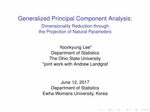
Variance Maximization

I Given p correlated variables X = (X1, · · · ,Xp)>, consider alinear combination of Xj ’s,

p∑j=1

ajXj = a>X

for a = (a1, . . . ,ap)> ∈ Rp with ‖a‖2 = 1.

I The first principal component direction is defined as thevector a that gives the largest sample variance of a>Xamong all unit vectors a:

maxa∈Rp,‖a‖2=1

a>Sna

where Sn is the sample variance-covariance matrix of X .

Principal Components

I Let Sn =∑p

j=1 λjvjv>j with eigenvaluesλ1 ≥ λ2 ≥ · · · ≥ λp > 0, and the correspondingeigenvectors v1, . . . , vp.

I The first principal component direction is given by v1, andthe derived variable Z1 = v>1 X is called the first principalcomponent.

I In general, the j th principal component direction is definedsuccessively from j = 1 to p with orthogonality constraints.

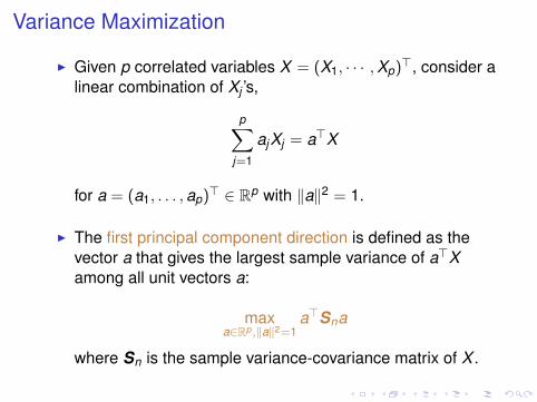
Pearson’s Reconstruction Error FormulationPearson, K. (1901), On Lines and Planes of Closest Fit toSystems of Points in Space

I Given x1, · · · , xn ∈ Rp, consider the data approximation

xi ≈ µ+ vv>(xi − µ)

where µ ∈ Rp and v is a unit vector in Rp so that vv> is arank-one projection.

I What are µ and v ∈ Rp (with ‖v‖2 = 1) that minimize thereconstruction error?

n∑i=1

‖xi − µ− vv>(xi − µ)‖2

I µ̂ = x̄ and v̂ = v1 minimize the error.

Minimization of Reconstruction Error

I More generally, consider a rank-k (< p) approximation:

xi ≈ µ+ VV>(xi − µ)

where µ ∈ Rp and V is a p × k matrix with orthogonalcolumns that results in a rank-k projection of VV>.

I Wish to minimize the reconstruction error:

n∑i=1

‖xi − µ− VV>(xi − µ)‖2

subject to V>V = Ik

I µ̂ = x̄ and V̂ = [v1, · · · , vk ] provide the best k -dimensionalreconstruction of the data.

PCA for Non-Gaussian Data?

I PCA finds a low rank subspace by implicitly minimizing thereconstruction error under squared error loss, which islinked to the Gaussian distribution.

I Binary, count, or non-negative data abound in practice.

e.g. images, term frequencies for documents, ratings formovies, click-through rates for online ads

I How to generalize PCA to non-Gaussian data?

Generalization of PCACollins et al. (2001), A generalization of principal componentsanalysis to the exponential family

I Draws on the ideas from the exponential family andgeneralized linear models.

I For Gaussian data, assume that xi ∼ Np(θi , Ip) and θi ∈ Rp

lies in a k dimensional subspace:

for a basis {b`}k`=1, θi =k∑

`=1

ai`b` = B(p×k)ai

I To find Θ = [θij ], maximize the log likelihood or equivalentlyminimize the negative log likelihood (or deviance):

n∑i=1

‖xi − θi‖2 = ‖X −Θ‖2F = ‖X − AB>‖2F

Generalization of PCAI According to Eckart-Young theorem, the best rank-k

approximation of X (= Un×pDp×pV>p×p) is given by therank-k truncated singular value decomposition UkDk︸ ︷︷ ︸

A

V>k︸︷︷︸B>

.

I For exponential family data, factorize the matrix of naturalparameter values Θ as AB> with rank-k matrices An×k andBp×k (of orthogonal columns) by maximizing the loglikelihood.

I For binary data X = [xij ] with P = [pij ], “logistic PCA” looks

for a factorization of Θ =[log pij

1−pij

]= AB> that maximizes

`(X ; Θ) =∑i,j

{xij(a>i bj∗)− log(1 + exp(a>i bj∗))

}

subject to B>B = Ik .

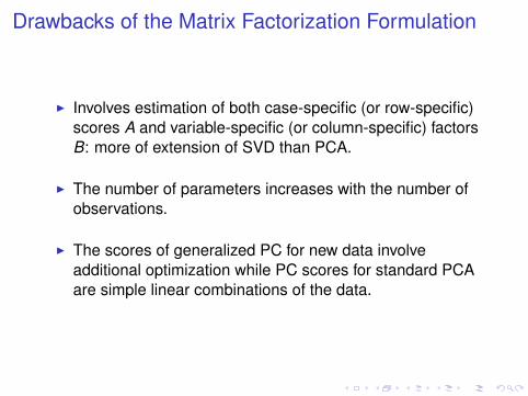
Drawbacks of the Matrix Factorization Formulation

I Involves estimation of both case-specific (or row-specific)scores A and variable-specific (or column-specific) factorsB: more of extension of SVD than PCA.

I The number of parameters increases with the number ofobservations.

I The scores of generalized PC for new data involveadditional optimization while PC scores for standard PCAare simple linear combinations of the data.

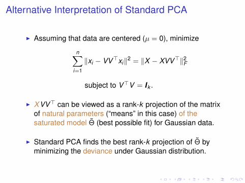
Alternative Interpretation of Standard PCA

I Assuming that data are centered (µ = 0), minimize

n∑i=1

‖xi − VV>xi‖2 = ‖X − XVV>‖2F

subject to V>V = Ik .

I XVV> can be viewed as a rank-k projection of the matrixof natural parameters (“means” in this case) of thesaturated model Θ̃ (best possible fit) for Gaussian data.

I Standard PCA finds the best rank-k projection of Θ̃ byminimizing the deviance under Gaussian distribution.

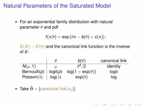
Natural Parameters of the Saturated Model

I For an exponential family distribution with naturalparameter θ and pdf

f (x |θ) = exp (θx − b(θ) + c(x)) ,

E(X ) = b′(θ) and the canonical link function is the inverseof b′.

θ b(θ) canonical linkN(µ,1) µ θ2/2 identityBernoulli(p) logit(p) log(1 + exp(θ)) logitPoisson(λ) log(λ) exp(θ) log

I Take Θ̃ = [canonical link(xij)].

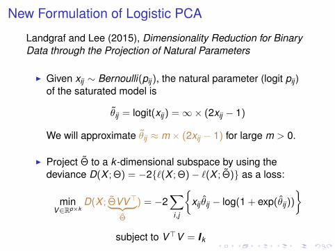
New Formulation of Logistic PCA

Landgraf and Lee (2015), Dimensionality Reduction for BinaryData through the Projection of Natural Parameters

I Given xij ∼ Bernoulli(pij), the natural parameter (logit pij )of the saturated model is

θ̃ij = logit(xij) =∞× (2xij − 1)

We will approximate θ̃ij ≈ m × (2xij − 1) for large m > 0.

I Project Θ̃ to a k -dimensional subspace by using thedeviance D(X ; Θ) = −2{`(X ; Θ)− `(X ; Θ̃)} as a loss:

minV∈Rp×k

D(X ; Θ̃VV>︸ ︷︷ ︸Θ̂

) = −2∑i,j

{xij θ̂ij − log(1 + exp(θ̂ij))

}

subject to V>V = Ik

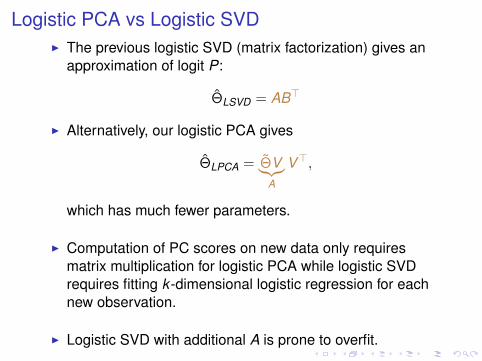
Logistic PCA vs Logistic SVDI The previous logistic SVD (matrix factorization) gives an

approximation of logit P:

Θ̂LSVD = AB>

I Alternatively, our logistic PCA gives

Θ̂LPCA = Θ̃V︸︷︷︸A

V>,

which has much fewer parameters.

I Computation of PC scores on new data only requiresmatrix multiplication for logistic PCA while logistic SVDrequires fitting k -dimensional logistic regression for eachnew observation.

I Logistic SVD with additional A is prone to overfit.

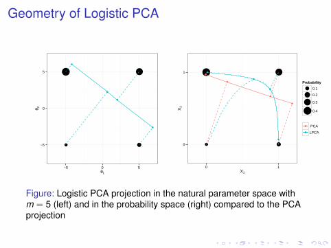
Geometry of Logistic PCA

● ●

●

●

●

●

●

−5

0

5

−5 0 5θ1

θ 2

● ●

●●

●

●

●

●

●

●

●

0

1

0 1X1

X2

Probability

●

●●●

0.1

0.2

0.3

0.4

●●

●●

PCA

LPCA

Figure: Logistic PCA projection in the natural parameter space withm = 5 (left) and in the probability space (right) compared to the PCAprojection

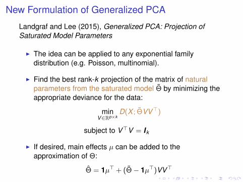
New Formulation of Generalized PCA

Landgraf and Lee (2015), Generalized PCA: Projection ofSaturated Model Parameters

I The idea can be applied to any exponential familydistribution (e.g. Poisson, multinomial).

I Find the best rank-k projection of the matrix of naturalparameters from the saturated model Θ̃ by minimizing theappropriate deviance for the data:

minV∈Rp×k

D(X ; Θ̃VV>)

subject to V>V = Ik

I If desired, main effects µ can be added to theapproximation of Θ:

Θ̂ = 1µ> + (Θ̃− 1µ>)VV>

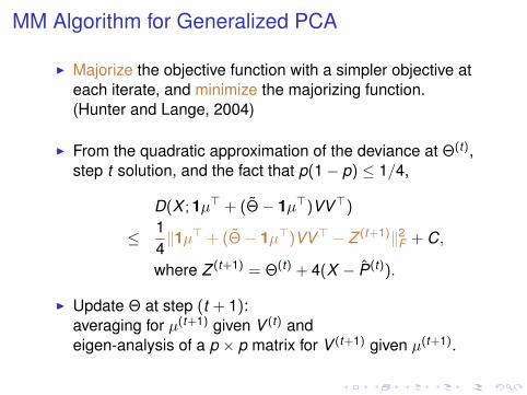
MM Algorithm for Generalized PCA

I Majorize the objective function with a simpler objective ateach iterate, and minimize the majorizing function.(Hunter and Lange, 2004)

I From the quadratic approximation of the deviance at Θ(t),step t solution, and the fact that p(1− p) ≤ 1/4,

D(X ; 1µ> + (Θ̃− 1µ>)VV>)

≤ 14‖1µ> + (Θ̃− 1µ>)VV> − Z (t+1)‖2F + C,

where Z (t+1) = Θ(t) + 4(X − P̂(t)).

I Update Θ at step (t + 1):averaging for µ(t+1) given V (t) andeigen-analysis of a p × p matrix for V (t+1) given µ(t+1).

Medical Diagnosis Data

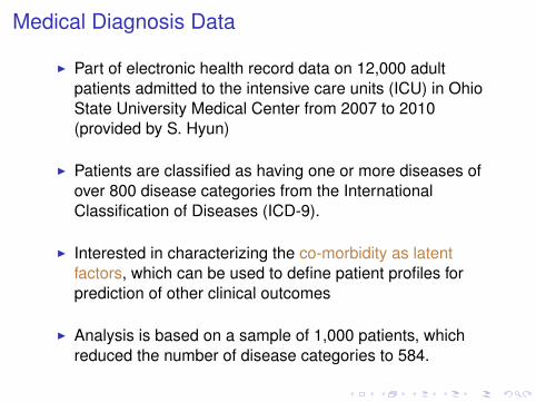
I Part of electronic health record data on 12,000 adultpatients admitted to the intensive care units (ICU) in OhioState University Medical Center from 2007 to 2010(provided by S. Hyun)

I Patients are classified as having one or more diseases ofover 800 disease categories from the InternationalClassification of Diseases (ICD-9).

I Interested in characterizing the co-morbidity as latentfactors, which can be used to define patient profiles forprediction of other clinical outcomes

I Analysis is based on a sample of 1,000 patients, whichreduced the number of disease categories to 584.

Patient-Diagnosis Matrix

Deviance Explained by Components

●

●●

●●

●●

●●

●●

●●

●●

●●

●●

●●

●●●●●●●●●● ●

●

●●●

●●●●●●

●●●●●●●

●●●

●●

●●

●●●●●

Cumulative Marginal

0%

25%

50%

75%

0.0%

2.5%

5.0%

7.5%

0 10 20 30 0 10 20 30Number of Principal Components

% o

f Dev

ianc

e E

xpla

ined

●

LPCA

LSVD

PCA

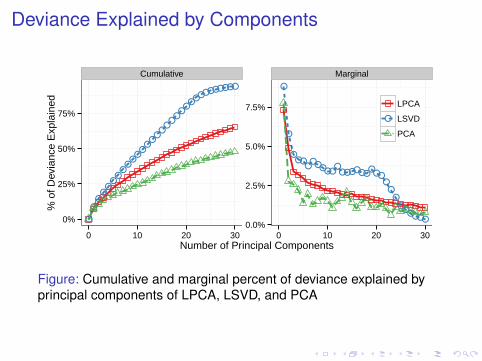
Figure: Cumulative and marginal percent of deviance explained byprincipal components of LPCA, LSVD, and PCA

Deviance Explained by Parameters

0%

25%

50%

75%

0k 10k 20k 30k 40kNumber of free parameters

% o

f dev

ianc

e ex

plai

ned

LPCA

LSVD

PCA

Figure: Cumulative percent of deviance explained by principalcomponents of LPCA, LSVD, and PCA versus the number of freeparameters

Predictive Deviance

●

●●●●●●●●●●●●●●●●●●●●●●●●●●●●●●

●

●●

●

●

●●●

●●

●

●●

●

●

●

●●●

●●

●

●

●

●●

●●●

●

Cumulative Marginal

0%

10%

20%

30%

40%

0%

2%

4%

6%

0 10 20 30 0 10 20 30Number of principal components

% o

f pre

dict

ive

devi

ance

●

LPCA

PCA

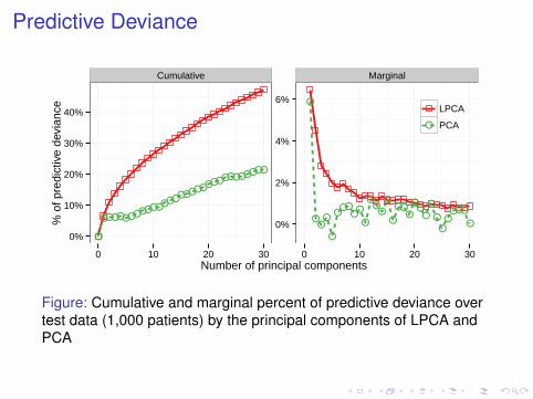
Figure: Cumulative and marginal percent of predictive deviance overtest data (1,000 patients) by the principal components of LPCA andPCA

Interpretation of Loadings

●

●●

●● ●

●

●

●● ●

●

●

●

●●

●

●

●●

●

●● ● ●● ●

● ●●

● ● ●

● ●

●

●

●

●

●

●

●

●

●

●

●●

●

●●

●●

● ●

●

●●

●

●

●

● ● ●

●

●●

●

●●

●●

●

●

●

●

●

●

●

●

●

●

●

●

●●

●●

●●

●

●

● ●

●

●

● ●●

●

●

●

●●

●

●

●

●

●

●

●

●

●

●●

●

●

●

●

●

●●

●

●

●

●

●

●●

●●●

●

●

●

●

●● ●

●

●

●

● ●

●

●

●●

●

●

●

●

●●

●

●

●

●

●

●●

●

●

●

●

●

●

●

●●

● ●● ●

●

●

●●

●

●

● ●

●

●

● ●●● ●

●●

●●

●●

●●●

●

● ●

●

●

●

●

●

●

●

●

●

●

●

●

●

●

●

●

●

●

●

●

●

●

●

●

●

●

●

●

●

●

●

●

●

●

●

●

● ●● ●

●

●

●

●

●

●

●

● ●

●

●

●●

●●

●●

●

● ●

●

●●●

●

●

●

●

●

●●

●

●

●

●

●

●

●

●●

●

●●

●●

●

●●

●

●

●

●

●

●●

●

● ●●

●

●

●● ●

●

●

●

●

●

●

●

●

●

●

●●

●

●●

●

●

●

●●●●

●

●

●

●

●

●

● ●●

●● ● ●

●

●

●●

●● ●●

●●

● ●●● ● ● ●● ●●

●●●

●

●●●

● ●

● ●●●●●

●

●●

●●

●●

●●

●

●●

●

●

●

●

●

●

●

●

●●

●

●●

●

●●

●

●

●

●●

●●

●

●

●●

●●

●

●

●●●●

●

●

●●

●● ●●

●●●

●●● ●

● ●● ●●●●

●●● ●

●●●●

●

● ● ●●●

●

●●

●

● ●●

● ●●● ●●●●

●

●●

● ●●●

●

●●● ●●

●●

●●

●●●

●●

●

●

●

●

●●●

●

● ●●●

●●

● ●● ●

●

●

●

●

●

●

●

●●

●

●

● ●●

●

●

●

● ●

●

●

●●

●

●●

●●

●

● ● ●

●

●●

●

●

●

●●

●

●●

●●

●

●

●

●

●

●

●●

●●

●●

●

●

●

●

●

●●● ●

●

● ●●

●

●

●

●

●●

●●

●

●

●

●

●

●

●

●●

●

●● ●

●

●

●

●

●

●

● ●●

●

●●

●

●●

●

●

●

● ●

●

●●●

● ●●

● ●

●

● ●●●

●

●

●

●●

●

●

●

●

●

●

● ●

●

●

●

●

●●

●

●●

●●

●

●● ●●

●

●

●

●

●

● ●

●●

●

●

●

●

●

●● ●

●

●

●

●

●

●

●

●●

●

●

●

●

●

●

●

●

●●

●

●

●

●

●

●

●

●

●

●

●

●

●

●

● ●●●

●●

●

● ●

●

●

●

●

● ●

●

●

●

● ●

●

●●

●

●

●

●

●

●●

● ●

●

●●

●

●●

●

●● ●

●

●

●

●●● ● ●

●●

●

●

●

●●

●

●

●

●

●

●

●

●

●

●

●

●

●

●

●

●

●

●

●

●

●

●

●

●

●●

●

●

●

●

●●

●

●

●

●

●●● ●

●

●

●

●

●

●

●●

●●

●

●

●

●

●

●

●

●

●●

●

●●

●

●

●

●

●

●

●●

●

●●

●●

●

●

●● ●

●

●● ●

●

● ●● ●

●

●●

●

●

●

●

●

●

● ●

●

●

● ●●

●

●

●

●

●

●

●

●

●●

●

●

●

●

●●

●

●

●●

●

●

●

●

●

●

●

●

●

●●

●

●

●

●●

●●●●

●●● ●●● ●● ● ●● ●● ● ●

●

●

●●

●

●●●

●

●●●

●

●

●

●

●

●

●

●●

●

●

●

●

●

●

●

●●

●

●

●

●

●

●●●

●

●

●

●●●●

●●

●

●

●

●

●

●

●

●●

●●

●

●

●

●

●

●

● ● ●

●

●

●

●

●●

●

●

●

● ●

●

●

●

● ●

●

●●

●

●

●

●

●●

●

●

●

●●

●●

●●

●

●

●

●

●

●●

●

● ●● ●

●

●●

●

●● ●●● ●● ●

●●

●

●

●●●● ●

●●

●

●●

●● ●

●●●

●

●

●

●●

●●●

●

●

●

●●●

●

●●● ●

●●●●

●

●

●

●

●

●

● ●●

●

●

● ●

●

●

●●

● ●●

●

●

●

●

●●

●

●

●● ●

●

●

●

●

● ●●●

●

●

●● ●

●

●

●

●

● ●

01:Gram−neg septicemia NEC03:Hyperpotassemia

08:Acute respiratry failure

10:Acute kidney failure NOS16:Speech Disturbance NEC

17:Asphyxiation/strangulat

03:DMII wo cmp nt st uncntr

03:Hyperlipidemia NEC/NOS

04:Leukocytosis NOS

07:Mal hy kid w cr kid I−IV

07:Old myocardial infarct

07:Crnry athrscl natve vssl

07:Systolic hrt failure NOS

09:Oral soft tissue dis NEC

10:Chr kidney dis stage IIIV:Gastrostomy status

−0.2

0.0

0.2

Component 1 Component 2

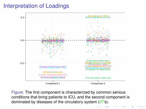
Figure: The first component is characterized by common seriousconditions that bring patients to ICU, and the second component isdominated by diseases of the circulatory system (07’s).

Concluding Remarks

I We have generalized PCA via projections of the naturalparameters of the saturated model using the generalizedlinear model framework.

I We have extended generalized PCA to handle differentialcase weights, missing data, and variable normalization.

I Further extensions are possible with other constraints thanrank for desirable properties (e.g. sparsity) on the loadingsand predictive formulations.

I R package, logisticPCA is available at CRAN andgeneralizedPCA is currently under development.

Acknowledgments

Andrew Landgraf@ Battelle Memorial Institute

Sookyung Hyun and Cheryl Newton@ College of Nursing, OSU

DMS-15-13566

References

A. J. Landgraf and Y. Lee.Dimensionality reduction for binary data through the projection ofnatural parameters.Technical Report 890, Department of Statistics, The Ohio StateUniversity, 2015.Also available at arXiv:1510.06112.

A. J. Landgraf and Y. Lee.Generalized principal component analysis: Projection ofsaturated model parameters.Technical Report 892, Department of Statistics, The Ohio StateUniversity, 2015.